the risk of pythium aphanidermatum in hydroponic baby-leaf
TRANSCRIPT

THE RISK OF PYTHIUM APHANIDERMATUM IN
HYDROPONIC BABY-LEAF SPINACH PRODUCTION
A Dissertation
Presented to the Faculty of the Graduate School
of Cornell University
In Partial Fulfillment of the Requirements for the Degree of
Doctor of Philosophy
by
Timothy James Shelford
May 2010

© 2010 Timothy James Shelford

THE RISK OF PYTHIUM APHANIDERMATUM IN
HYDROPONIC BABYLEAF SPINACH PRODUCTION
Timothy James Shelford, Ph. D.
Cornell University 2010
Pythium aphanidermatum has been identified as the main obstacle/risk in the
production of hydroponically grown babyleaf spinach. This organism is so prevalent
that even crops grown in fresh nutrient solution will often show signs of Pythium
damage at harvest time. Previous studies have identified nutrient solution temperature
as a key factor in determining the growth and development of Pythium.
The goal of this study was to estimate the risk of Pythium outbreaks under
different hydroponic production strategies. To provide these estimates, a greenhouse
simulation model was coupled with a spinach growth and Pythium disease model.
Through Monte-Carlo simulation, estimates of the time between and the seasonality of
outbreaks were determined. The strategies modeled included using nutrient solution
temperatures of 18, 20, 22, 24C and unregulated temperature. Within these
temperature regimes different harvesting schedules were examined. Assuming
supplemental lighting control to a daily light integral of 17 mol m-2
, crop durations of
12, 14 and 16 days in pond were examined. To quantify the importance of
supplemental lighting, crop durations were replaced with target harvest biomasses.
The target harvest biomasses were then achieved without supplemental lighting. A
further strategy examined within the fixed duration conditions was the use of a two
pond system where crop cohorts older than half the total crop duration were moved to
a separate pond.

A nutrient solution temperature of 18C with a 12 day crop duration resulted in
an expected frequency of Pythium outbreak of 0.032 per year, compared to 1.47
outbreaks per year for a 16 day crop grown without nutrient solution temperature
control. The same conditions without supplemental lighting resulted in outbreaks
frequencies of 7.9 per year and 16 per year respectively. Under a two pond system
the expected frequency of outbreak was approximately halved at 18C and increased
with increasing temperature until there was no difference between the one and two
pond systems for the uncontrolled temperature conditions.

iii
BIOGRAPHICAL SKETCH
Timothy Shelford was born in Vancouver, BC in 1974 to Helen and James
Shelford. He graduated from Point Grey Highschool in 1992. He then did his
undergraduate studies at the University of British Columbia in the department of
Bioresource Engineering, and graduated with a B.A.Sc. with distinction in 1997.
Timothy then completed a Masters of Applied Science in Bioresource
Engineering at the University of British Columbia, in 2000. His project investigated
different ways of scheduling irrigation in greenhouse tomato production, with the aim
of conserving water and nutrients. Following his Masters degree he worked as an
environmental engineer at Entech Environmental Consultants in West Vancouver, BC.
Projects included contaminated site investigations and powder post beetle assessment
and abatement in historic wooden structures.
During his youth he worked at a variety of agricultural jobs from picking
raspberries and selling sweet corn on his uncle‟s farm, to an animal technician on the
Agriculture Canada greenbelt research farm in Ottawa ON, and as a research associate
on a fish farm research project on Quadra Island, BC.
In 2002 Timothy was accepted into the Cornell Controlled Environment
Agriculture program in the department of Biological and Environmental Engineering
at Cornell University. During his time at Cornell he worked as a teaching assistant in
several courses including, Introductory computer programming, Heat, Mass and
Momentum Transfer, and Bioinstrumentation. He also worked on a variety of projects
related to hydroponic spinach production. In 2007 he began working for CEA
Systems Inc, developing a supplemental light, shade and CO2 control algorithm
developed by his advisor Professor Louis Albright.
His hobbies include collecting tools for home improvement projects, keeping
various ancient computers running and travel in general.

iv
DEDICATION
This research is dedicated to my father who passed away in 2002, and my
mother whose unquestioning love and support have made everything I‟ve done
possible.

v
ACKNOWLEDGEMENTS
I would like to thank the members of my committee Dr. Louis Albright, Dr.
Robert Langhans, and Dr. Jery Stedinger for their support and guidance through my
dissertation. I would also like to thank the department of Biological and
Environmental engineering for their generous support through a fellowship in my first
year, and teaching assistantships throughout my time at Cornell (particularly
Bioinstrumentation with Dr. Daniel Aneshansley.) In addition CEA Systems Inc has
supported me through the LASSI2 SBIR project phases one and two.
Over the years I‟ve become good friends with the members of the staff at KPL
and Riley-Robb Hall, and have relied on the friendship and support of fellow CEA
members Melissa and David.
A listing of all my friends, who provided encouragement, support and sanity
preserving distraction would fill volumes two and three of this dissertation and would
still not be complete.
I also couldn‟t have done it without all the support and encouragement my
family has heaped on me. Particularly from my mother Helen, my aunt Valerie and
my brothers Jeremy and Mark.

vi
TABLE OF CONTENTS
Biographical Sketch ....................................................................................................... iii
Dedication ...................................................................................................................... iv
Acknowledgements ........................................................................................................ v
List of Figures .............................................................................................................. viii
List of Tables ............................................................................................................... xiv
Chapter 1: Introduction ................................................................................................... 1
1.1 Background ........................................................................................................... 1
1.2 Research Objectives: ............................................................................................. 4
1.3 Research Approach ............................................................................................... 5
Chapter 2: Bench-top Evaluation of Management Options ........................................... 8
2.1 Introduction ........................................................................................................... 8
2.2 Methods and Materials .......................................................................................... 9
2.3 Results and Discussion ....................................................................................... 15
2.4 Conclusions ......................................................................................................... 22
Chapter 3: Continuous Production Experiments .......................................................... 25
3.1 Introduction ......................................................................................................... 25
3.2 Methods and materials ........................................................................................ 27
3.3 Results and Discussion ....................................................................................... 30
3.4 Conclusions ......................................................................................................... 35
Chapter 4: Greenhouse Temperature Simulation Model .............................................. 36
4.1 Introduction: ........................................................................................................ 36
4.2 Literature Review: .............................................................................................. 38
4.3 Methods and Materials: ...................................................................................... 40
4.4 Results: ................................................................................................................ 86
4.5 Discussion: .......................................................................................................... 92
Chapter 5: Spinach Growth Model ............................................................................... 94
5.1 Introduction: ........................................................................................................ 94
vii
5.2 Literature Review: .............................................................................................. 95
5.3 Methods and Materials: ...................................................................................... 97
5.4 Results: .............................................................................................................. 113
5.5 Discussion: ........................................................................................................ 118
Chapter 6: Pythium Aphanidermatum Growth and Transmission Model .................. 122
6.1 Introduction: ...................................................................................................... 122
6.2 Literature Review: ............................................................................................ 123
6.3 Methods and Materials: .................................................................................... 127
6.4 Results: .............................................................................................................. 157
6.5 Discussion: ........................................................................................................ 186
Chapter 7: Simulation of Select Production Strategies .............................................. 192
7.1 Introduction: ...................................................................................................... 192
7.2 Literature Review: ............................................................................................ 195
7.3 Methods and Materials: .................................................................................... 202
7.4 Results: .............................................................................................................. 215
7.5 Discussion: ........................................................................................................ 224
Chapter 8: Conclusions ............................................................................................... 229
Appendix .................................................................................................................... 235
Bibliography ............................................................................................................... 290
viii
LIST OF FIGURES
Figure 2.1 Spinach seedling bioassay before application of solution of
interest. 10
Figure 2.2 Electrochemical pH adjustment apparatus. 12
Figure 2.3 Average root damage due to varying concentration of
Pythium (Error bars are ± 1 SE) 16
Figure 2.4 Fraction damage reduction due to Electrochemcial
Treatment 18
Figure 2.5 Fraction damage reduction due to Pasteurization 19
Figure 2.6 Fraction damage reduction due to Sonication 20
Figure 2.7 Fraction reduction due to Ultraviolet Sterilization 21
Figure 3.1 Overview photograph of spinach growing benches used in
the multi-cohort evaluation of filtration, UV sterilization and
temperatures suppression in continuous production. 28
Figure 3.2 Average plant fresh weights at time of harvest in control
benches 31
Figure 3.3 Roots of uninfected (left) and infected (right) flats 31
Figure 3.4 Average plant fresh weight in the filtration, control
(uninoculated) and inoculated systems, at time of harvest. 32
Figure 3.5 Average plant fresh weight in the Ultraviolet systems at
time of harvest 33
Figure 3.6 Average Plant fresh weight in the temperature depression
systems at harvest. 34
Figure 4.1 Diagram of thermal layers and energy flow processes within
the greenhouse model. 43
Figure 4.2 Model temperatures with a common initial temperature and
no heat inputs/outputs. 87
Figure 4.3 Temperatures of the greenhouse simulation model layers as
a function of time when the initial temperature of the pond is set to 35C
and the remaining layers to 24C. 88

ix
Figure 4.4 Effect of heating (24/19 day/night setpoint) on simulated
greenhouse air temperature during a typical cold, dark winter day. 89
Figure 4.5 Effect of pad cooling and venting on greenhouse air
temperatures (24/19 day/night setpoint) during a typical warm sunny
day. 90
Figure 4.6 Simulated Pond temperatures over the course of the year
using 1988 weather data from Ithaca, NY. 91
Table 5.1 Symbols and definitions of parameters and variables used in
the modified SUCROS hourly spinach growth model. 101
Figure 5.1 Leaf Area Index during spinach crop cycle (1200 plants m-
2) 111
Figure 5.2 Leaf Area Index as a function of leaf mass. 111
Figure 5.3 Simulated Leaf Dry Mass Growth over first 48 hours with
LASSI controlled lighting to a daily integral of 19.2 mols m-2
. 115
Figure 5.4 Measured and simulated leaf dry mass over the course of
the crop cycle. Grown with 19.2 mol m-2
day-1
PAR. 116
Figure 5.5 Tornado plot of the effect of varying model parameters +/-
10% on the simulated crop biomass (kg/ha) at harvest day 16. 117
Figure 6.1 Disease cycle of Pythium sp. (Agrios 1978). 124
Figure 6.2 Mycelium growth rate as a function of the average
uninfected root mass. 138
Figure 6.3 Sum of the Squared Error of the fraction shoot biomass
reduction as a function of the coefficient of photosynthetic rate
reduction (ηphoto). 143
Figure 6.4 Normalized Pythium damage as a function of initial
concentration of zoospores. (Data from Katzman). 145
Figure 6.5 Age adjustment factor as a function of nutrient solution
temperature. 148
Figure 6.6 Zoospore release amount as a function of zoospore release
age 153
Figure 6.7 Yield ratio (infected biomass/uninfected biomass value).
From Katzman (2003) observed time of inoculation experiment and
x
model predictions (with and without reinfection) at a root zone
temperature of 24C. Code is I, followed by inoculation day, and H,
followed by harvest day. 159
Figure 6.8 Fraction of roots infected. From Katzman's observed time
of inoculation experiment and model predictions (with and without
reinfection). Code is I, followed by inoculation day, and H, followed by
harvest day. 159
Figure 6.9 Fraction of roots dark brown/black. From Katzman's
observed time of inoculation experiment and model predictions (with
and without reinfection). Code is I, followed by inoculation day, and H,
followed by harvest day. 160
Figure 6.10 Yield ratio (infected biomass/uninfected biomass value),
fraction of roots infected (Frac infected), and fraction of roots dark
brown/black Frac DB/B). From Katzman's observed temperature and
zoospore concentration experiments (24 C and 25 zoos ml-1
) and model
predictions. 161
Figure 6.11 Yield ratio (infected biomass/uninfected biomass value) at
harvest. From Katzman's nutrient solution temperature experiment and
model predictions. Code is temperature followed by harvest day. 162
Figure 6.12 Fraction of root infected. From Katzman's nutrient
solution temperature experiment, and model predictions. Code is
temperature followed by harvest day. 163
Figure 6.13 Fraction of root dark brown/black. From Katzman's
nutrient solution temperature experiment, and model predictions. Code
is temperature followed by harvest day. 163
Figure 6.14 Yield ratio (infected biomass/uninfected biomass value) at
harvest. From Katzman's uninoculated nutrient solution temperature
experiment, and model predictions. Code is temperature followed by
harvest day. 165
Figure 6.15 Fraction of root infected. From Katzman's uninoculated
nutrient solution temperature experiment, and model predictions. Code
is temperature followed by harvest day. 166
Figure 6.16 Fraction of root dark brown/black. From Katzman's
uninoculated nutrient solution temperature experiment, and model
predictions. Code is temperature followed by harvest day. (Note scale
is different from other figures.) 166
xi
Figure 6.17 Yield ratio (infected biomass/uninfected biomass value) at
harvest. From Katzman's inoculation concentration experiment, and
model predictions. Code is zoospore concentration (zoos ml-1
)
followed by harvest day. 167
Figure 6.18 Fraction of roots infected. From Katzman's inoculation
concentration experiment, and model predictions. . Code is zoospore
concentration (zoos ml-1
) followed by harvest day. 168
Figure 6.19 Fraction of root dark brown/black. From Katzman's
inoculation concentration experiment, and model predictions. . Code is
zoospore concentration (zoos ml-1
) followed by harvest day. 168
Figure 6.20 Yield ratio (infected biomass/uninfected biomass value)
for a warm temperature nutrient solution (27.5C) inoculated with 100
zoos ml-1
for one sequence of harvests. (A new cohort was added every
3 days, harvested after 14 days for a total experimental time of 41
days.) 170
Figure 6.21 Yield ratio of biomasses (infected/uninfected) for an
initially warm temperature nutrient solution (27.5C) inoculated with
100 zoos ml-1, switched to a cold (20C) temperature nutrient solution,
24 hours after inoculation. 171
Figure 6.22 Sensitivity of the fraction of uninfected biomass to model
parameters with inoculation on day 1 and harvest on day 9 with a
nutrient solution of 24 C. 175
Figure 6.23 Sensitivity of the fraction of uninfected roots to model
parameters with inoculation on day 1 and harvest on day 9 with a
nutrient solution of 24 C. 175
Figure 6.24 Sensitivity of the fraction of roots dark brown/black to
model parameters with inoculation on day 1 and harvest on day 9 with
a nutrient solution of 24 C. 176
Figure 6.25 Sensitivity of the fraction of uninfected biomass to model
parameters with inoculation on day 1 and harvest on day 14 with a
nutrient solution of 24 C. 176
Figure 6.26 Sensitivity of the fraction of uninfected roots to model
parameters with inoculation on day 1 and harvest on day 14 with a
nutrient solution of 24 C. 177
Figure 6.27 Sensitivity of the fraction of roots dark brown/black to
model parameters with inoculation on day 1 and harvest on day 14 with
a nutrient solution of 24 C. 177

xii
Figure 6.28 Sensitivity of the fraction of uninfected biomass to model
parameters with inoculation on day 1 and harvest on day 21 with a
nutrient solution of 24 C. 178
Figure 6.29 Sensitivity of the fraction of uninfected roots to model
parameters with inoculation on day 1 and harvest on day 21 with a
nutrient solution of 24 C. 178
Figure 6.30 Sensitivity of the fraction of roots dark brown/black to
model parameters with inoculation on day 1 and harvest on day 21 with
a nutrient solution of 24 C. 179
Figure 6.31 Sensitivity of the fraction of uninfected biomass to model
parameters with inoculation on day 9 and harvest on day 14 with a
nutrient solution of 24 C. 179
Figure 6.32 Sensitivity of the fraction of uninfected roots to model
parameters with inoculation on day 9 and harvest on day 14 with a
nutrient solution of 24 C. 180
Figure 6.33 Sensitivity of the fraction of roots dark brown/black to
model parameters with inoculation on day 9 and harvest on day 14 with
a nutrient solution of 24 C. 180
Figure 6.34 Sensitivity of the fraction of uninfected biomass to model
parameters with inoculation on day 9 and harvest on day 21 with a
nutrient solution of 24 C. 181
Figure 6.35 Sensitivity of the fraction of uninfected roots to model
parameters with inoculation on day 9 and harvest on day 21 with a
nutrient solution of 24 C. 181
Figure 6.36 Sensitivity of the fraction of roots dark brown/black to
model parameters with inoculation on day 9 and harvest on day 21 with
a nutrient solution of 24 C. 182
Figure 6.37 Sensitivity of the fraction of uninfected biomass to model
parameters at harvest day 21 with no inoculation and a nutrient solution
of 24 C. 183
Figure 6.38 Sensitivity of the fraction of the root infected to model
parameters at harvest day 21 with no inoculation and a nutrient solution
of 24 C. 183
Figure 6.39 Sensitivity of the fraction of the root dark brown/black to
model parameters at harvest day 21 with no inoculation and a nutrient
solution of 24 C. 184

xiii
Figure 6.40 Sensitivity of the fraction of uninfected biomass to model
parameters at harvest day 21 with no inoculation and a nutrient solution
of 30 C. 184
Figure 6.41 Sensitivity of the fraction of the root infected to model
parameters at harvest day 21 with no inoculation and a nutrient solution
of 30 C. 185
Figure 6.42 Sensitivity of the fraction of the root dark brown/black to
model parameters at harvest day 21 with no inoculation and a nutrient
solution of 30 C. 185
Figure 7.1 Leaf Area Index as a function of Leaf Biomass. Observed
values and predicted values with the best fit line slope increased and
decreased by 20%. Observed values from spinach crop harvested every
two days, with an average daily light integral of 19.2 mol m-2
. 209
Figure 7.2 Expected number of Pythium outbreaks per year, as a
function of nutrient solution temperature, and crop duration. For a one
pond (multi-cohort) production system with a daily light integral of 17
mols m-2
. 216
Figure 7.3 Pythium outbreaks by month, for the 24C nutrient solution
temperature, 16 day crop duration, and two pond condition. 217
Figure 7.4 Pythium outbreaks by month, for the 18C nutrient solution
temperature, and 16 day crop duration condition. 217
Figure 7.5 Pythium outbreaks by month, for the uncontrolled nutrient
solution temperature, and 16 day crop duration condition. 218
Figure 7.6 Expected number of Pythium outbreaks per year, as a
function of nutrient solution temperature, and crop duration. For a two
pond (multi-cohort) production system with a daily light integral of 17
mols m-2
. 220
Figure 7.7 Expected number of Pythium outbreaks per year, as a
function of nutrient solution temperature, and target crop harvest
biomass. For a one pond (multi-cohort) production system with no
supplemental light (natural daily light integral). 222
Figure 7.8 Effect of daily light integral (12, 17 and 22 mol m-2) on
harvest dry biomass with crop durations of 12, 14 and 16 days, in a
multi-cohort one pond system at 18C. 223

xiv
LIST OF TABLES
Table 4.1 Symbols, definition and values of parameters and variables
used in developing the energy flow equations of the lumped parameter
stepwise steady state greenhouse simulation model. 46
Table 5.1 Symbols and definitions of parameters and variables used in
the modified SUCROS hourly spinach growth model. 101
Table 5.2 Individual fresh weight, dry weight, leaf area and cumulated
PAR totals at each harvest day during spinach growth experiment. 114
Table 5.3 Predicted biomass as a function of daily light integral
compared to the baseline 19.2 mols with a production of 2565 kg/Ha at
16 days 117
Table 6.1 Summary of variables and symbols used in the Pythium
aphanidermatum growth and transmission model. 127
Table 6.2 Influence of time of inoculation on shoot dry mass of
spinach. Means and standard errors of shoot dry mass of plants
inoculated with P. aphanidermatum zoospores on different days (1, 9,
or 14) after sowing and harvested 9, 14, and 21 days after sowing.
(From Katzman) 133
Table 6.3 Percentages (%) of roots within each root rot category (1-4).
Spinach plants were inoculated with P. aphanidermatum zoospores on
different days (1, 9, or 14) after sowing and harvested 9, 14, and 21
days after sowing. (From Katzman) 133
Table 6.4 Estimated influence of time of inoculation on mycelium
infected root mass (g plant-1
) of spinach based on measured shoot dry
mass values, estimated root growth, and observed root condition.
(Measured values from Katzman) 137
Table 6.5 Percentages (%) of roots within each root rot rating (1-3) at
harvest. Spinach plants were inoculated with P. aphanidermatum
zoospores (0.025 to 250 per ml in 10-fold increments) 9 days after
seeding and harvested 14, and 21 days after seeding. (From Katzman) 144
Table 6.6 Influence of nutrient solution temperature and P.
aphanidermatum on shoot dry mass. Means and standard errors of
shoot dry mass (g per plant) for harvests at 9, 14, and 21 days after
seeding. Treatments varied nutrient solution temperatures (18, 24, and

xv
30 C) and presence or absence (+/−) of P. aphanidermatum (P.a.).
(From Katzman, 2003) 146
Table 6.7 Influence of nutrient solution temperature and inoculation
with P. aphanidermatum on root rot rating (RRR). Percentages (%) of
roots within each RRR category per treatment for plants harvested 14,
and 21 days after seeding. Treatments varied the nutrient solution
temperature (18, 24, and 30 C) and presence or absence (+/-) of P.
aphanidermatum (P.a.). (From Katzman) 147
Table 6.8 Influence of inoculation time, zoospore concentration and
temperature on zoospores detected in nutrient solution at time of
harvest. (From Katzman) 151
Table 6.9 Number of harvests (based on a 3 day harvest schedule in a
continuous production pond) before crop material is too badly damaged
by Pythium to market, as a function of nutrient solution temperature.
Grown at 18 to 32 C for 14 to 22 days. 172
Table 7.1 Simulated mean time between Pythium outbreaks severe
enough to require a cleanout. For a multi-cohort one pond system with
nutrient solution temperatures of 18C, 20C, 22C, 24C and uncontrolled,
and crop durations of 12, 14 and 16 days with a daily light integral of
17 mols m-2
PAR. (Simulation run for 500 years). 215
Table 7.2 Simulated mean time between Pythium outbreaks severe
enough to require a cleanout. For a multicohort two pond system with
nutrient solution temperatures of 18C, 20C, 22C, 24C and uncontrolled
and crop durations of 12, 14 and 16 days with a daily light integral of
17 mols m-2
PAR. Also included is the ratio of the mean time between
outbreaks for the two pond system over the one pond system. (500
years of simulation). 219
Table 7.3 Simulated mean time between Pythium outbreaks severe
enough to require a cleanout. For a multicohort one pond system with
nutrient solution temperatures of 18C, 20C, 22C, 24C and uncontrolled,
and target crop harvest biomasses (kg dry mass ha-1
) of 1186, 1534 and
1885 with no light integral control. (500 years of simulation). 221
Table 7.4 Effect of daily light integrals of 12, 17 and 22 mol m-2
on
Pythium outbreak frequency and harvest dry biomass, for a multi-
cohort one pond system with a nutrient solution temperature of 18C,
and crop durations of 12, 14 and 16 days. 223

1
CHAPTER 1: INTRODUCTION
1.1 BACKGROUND
Why hydroponic baby-leaf spinach?
The Controlled Environment Agriculture (CEA) Group at Cornell University
has focused on improving production techniques for existing greenhouse crops, and
developing production procedures for new crops. Through manipulating parameters
such as quantity and quality of light, CO2 concentration, aerial and root temperature,
and nutrient solution characteristics and composition, production times have been
decreased, productivity increased, and new production strategies have been passed on
to growers. With the success of producing greenhouse lettuce, focus has shifted to
looking at other similar crops that can benefit from greenhouse production,
particularly spinach.
A number of factors have driven the development of greenhouse hydroponic
spinach production. First is the increasing demand for baby spinach due to the
popularity of salad greens. Spinach is a crop rich in vitamins and nutrients, and baby-
leaf spinach is more tender than mature bunched spinach. Currently, spinach is
primarily produced through field production; however, there are a number of
drawbacks to such systems. The increasing cost of diesel has made shipping from
traditional production locales such as California and Florida more expensive. In
addition, leafy greens such as lettuce and spinach do not store and travel as well as
other produce such as tomatoes, cucumbers and peppers. Though lettuce and spinach
can be shipped, it is a race against time to get them to the consumer as quickly as
possible. Coupled with a public that wants to “eat local” this has led to the desire for
locally produced crops. To provide year round production in population dense areas
such as the Northeastern United States, greenhouses are the only option for local
production, due to the severity of winters.

2
Hydroponic greenhouse production makes more efficient use of valuable water
and nutrients. In field production, excess water and nutrients need to be applied,
which can lead to contamination of both aquifers and surface water. In addition, the
2006 recall of field grown spinach due to E.coli contamination highlighted the
inherent dangers of field production. Pathogens such as E. coli can be spread either
through animal or insect vectors as well as direct runoff and in aerosols of dust, and it
is extremely difficult to completely eliminate their threat from the field. Another
potential infection avenue is the washing stage which is necessary to remove the dirt,
grit and other residues including pesticides from the crop. Greenhouse spinach does
not need to be washed as it is grown in soilless culture and pesticides are not required.
An added benefit of removing the washing stage is increased shelf life as well as
removing another common avenue of food borne pathogen spread.
The demand for greenhouse hydroponic babyleaf spinach has led to
considerable research on growing techniques. However, to date there is no
commercial production in the United States, and there is limited production overseas.
The primary reason for this lack of production is the water mold Pythium
aphanidermatum (further referred to as Pythium). This organism is present in the
natural environment and attacks roots in a variety of field-grown crops. However, it is
particularly virulent in hydroponic production systems due to its ability to spread
through the nutrient solution. Its zoospores possess flagella that allow them to move
from root to root. This spread of disease is less of a problem in field conditions where
direct water paths are more limited. However, a highly mixed nutrient solution
provides ideal conditions for spread. Pythium zoospores attack the roots of a plant and
form mycelia that can release further zoospores or directly spread to other roots. In
addition to stunted growth, plants with Pythium damaged roots can wilt and even die
depending on the severity of the attack. In her doctoral dissertation, Katzman (2003)

3
investigated some of the factors that influence the progress of Pythium infections. To
expand on this work and to continue the development of hydroponic spinach
production, NYSERDA (New York State Energy Research and Development
Authority) commissioned a study (Albright et al., 2007) to investigate techniques for
controlling Pythium in the nutrient solution, focusing on traditional and novel water
sterilization techniques. As was found in this study, and previously recommended by
Katzman, the key to producing spinach is to manage, rather than attempt to completely
eliminate the disease. This dissertation seeks to apply the techniques of Risk Analysis
to arrive at recommendations for successfully producing hydroponic babyleaf spinach
in the presence of Pythium.
Why use Risk Analysis?
According to the Society of Risk Analysis (SRA, 2009), risk analysis is
defined as “Detailed examination of a facility, process, or materials that includes risk
assessment, risk evaluation, and risk management alternatives performed to
understand the nature of unwanted, negative consequences to human life, health,
property, or the environment; an analytical process to provide information regarding
undesirable events; or the process of quantification of the probabilities and expected
consequences for identified risks.“ Risk analysis is a systematic means of identifying,
assessing, and managing risk. The overall goals are to minimize losses, and to
maximize opportunities. These are precisely the goals of any farmer, and particularly
greenhouse growers who are faced with an organism such as Pythium.
The major steps involved in a risk analysis entail first identifying the risks that
face a particular endeavor, evaluating the likelihood of encountering these risks, and
then developing and implementing a management plan to minimize the impact of the
risks. This is also the procedure that the CEA program has taken in attempting to

4
develop hydroponic babyleaf spinach production. Following initial difficulties in
achieving consistent production, Katzman identified Pythium as the “root” cause. This
was backed up by other experiences described in the literature. Further experiments
and contact with other groups attempting to produce spinach hydroponically quickly
determined that the threat of Pythium is a problem of when, and not if, an outbreak
will happen. This assumption then led to the NYSERDA sponsored work to evaluate
techniques for dealing with Pythium, which relates to managing the risk. This
dissertation seeks to build on all of this work, to develop and test, in simulation,
management plans/production guidelines, to reduce the risk a grower faces when they
produce babyleaf spinach hydroponically.
1.2 RESEARCH OBJECTIVES:
The overall objective of this dissertation is to develop and use quantitative
methods to compare the risk of Pythium aphanidermatum infection in different
hydroponic baby spinach production systems and identify the least risky alternatives.
Such quantitative comparisons could then be used by a grower to determine which
production system suits their particular needs, and/or by a researcher interested in
further investigating/validating the risk of Pythium.
To achieve this objective a number of tasks were necessary:
1. to investigate current and non-traditional techniques for the control of Pythium
aphanidermatum in hydroponic nutrient solutions,
2. to apply the findings of the solution treatment techniques in the development
of production strategies,
3. to develop a linked greenhouse, crop, and disease model that can be used to
better understand the dynamics of a Pythium aphanidermatum infection, and to
simulate and evaluate different production strategies,

5
4. to simulate these production strategies under the greenhouse crop disease
model with crop damage metrics, in order to develop expected frequencies of
Pythium outbreak for each strategy.
1.3 RESEARCH APPROACH
Pythium aphanidermatum has been identified as the main obstacle/risk in the
production of hydroponically grown babyleaf spinach. This organism is so prevalent
that even crops grown in fresh nutrient solution will often show signs of Pythium
damage at harvest time. If this nutrient solution is subsequently reused for another
crop, the damage only multiplies.
In chapter two of this dissertation, new and existing water treatment
technologies were evaluated at a benchtop scale in an effort to manage infections by
destruction of Pythium zoospores. The results of this work were presented at the 2005
ASABE (American Society of Agricultural and Biological Engineers) annual
conference, and the paper was submitted to the conference proceedings (Shelford et
al., 2005). This work was funded by NYSERDA, and is also a part of the report made
to NYSERDA.
An experiment was then set up to test the promising technologies identified in
the benchtop work, and evaluate the performance of these technologies in actual
continuous production. The results of this work were presented at the 2006 ASABE
annual conference (Shelford et al., 2006), and make up chapter three of this
dissertation. This work was funded by NYSERDA and is also included in the final
report to NYSERDA.
The primary finding reported in the third chapter is that managing the disease
through crop cultural practices, rather than attempting to destroy Pythium zoospores in
solution, is the best way to deal with Pythium. Through a combination of reducing the

6
nutrient solution temperature to slow the reproduction rate of Pythium, and removal of
infected roots through short harvest cycles, it was shown that infections do not begin,
and that systems can recover from severe infections. Reducing nutrient solution
temperatures, and placing strict restrictions on the amount of time a crop can spend
growing, limits the flexibility available to a grower and imposes costs which may or
may not be acceptable. To determine the true limits of the system, a massive
experimental effort would be required, the results of which may or may not apply to
situations found outside of the Cornell greenhouses. It was decided that a simulation
of the greenhouse, crop and disease system would at least indicate the production
strategies which merit further investigation.
The fourth chapter of this dissertation provides a greenhouse thermal
environment model that uses the climate of the greenhouse location as input. Of
particular concern is the temperature of the nutrient solution, and the effects of
supplemental lighting and shading for crop daily light integral control on the
temperatures within the greenhouse, and the quality and timing of the light. A portion
of this program was used to assist in the evaluation of the LASSI2 (Light and Shade
System Implementation with CO2 supplementation) algorithm undertaken as a USDA
SBIR-funded project, in conjunction with CEA Systems Inc. In this dissertation the
greenhouse simulation model serves as an input to the spinach crop, and Pythium
disease models.
The fifth chapter uses data collected during the NYSERDA project, but not
included in the final report, of the growth of a spinach crop over time. Using this data,
the mechanistic growth model SUCROS (Goudriaan and van Laar, 1994) was adapted
to baby spinach production. SUCROS was selected as a framework for the growth
model because it differentiates the growth into root and shoot portions, and determines
the growth in these organs as a function of photosynthate production. It was felt that

7
such a model would be adaptable to modeling the effects of root damage due to
Pythium on the production of photosynthate, and hence on the growth of the entire
plant.
The sixth chapter of this dissertation uses the data Katzman collected to model
the effects of temperature, zoospore concentration, and time of inoculation on the
growth and spread of Pythium in a spinach crop. From this work, the parameters and
form of model necessary to describe an infection of Pythium were developed.
Because Katzman‟s work was in single crops of spinach, data collected during the
NYSERDA disease project was used to validate the model in multi-cohort common
nutrient solution use.
The seventh chapter ties the previous chapters together. The production
strategies suggested by the work of the third chapter are investigated through
simulation using the greenhouse model of chapter four, the crop growth model of
chapter five, and the Pythium disease model of chapter six. Thirteen years of
measured climate data for Ithaca, NY were used as the input for the greenhouse
simulation, and assumed distributions for the values of the crop growth, and Pythium
disease model parameters were used as input to a Monte-Carlo simulation of the
different production strategies. The results of the simulation are expected frequency
of Pythium outbreak for each production strategy. This information will provide
insight into production strategies to investigate further, before commercial adoption.

8
CHAPTER 2: BENCH-TOP EVALUATION OF MANAGEMENT OPTIONS
2.1 INTRODUCTION
Pythium aphanidermatum is arguably the largest hurdle to be overcome in the
development of commercial hydroponic spinach production systems. This ubiquitous
root disease organism can quickly spread through a crop, killing roots and devastating
production. Because this pathogen is waterborne, recirculating hydroponic systems
are ideally suited for quickly spreading the infection.
To suppress the dispersal of the organism, various treatment technologies have
been tried. Pasteurization and ultraviolet systems have demonstrated their ability to
successfully eliminate Pythium (Zhang and Tu, 2000, Runia et.al., 1988, Stanghellini
et al., 1984). However, there are drawbacks associated with their operation. Even
with the use of efficient heat exchangers, pasteurization is an energy intensive
operation that may not be feasible for large scale spinach production. Ultraviolet
radiation, though requiring less energy to achieve adequate Pythium destruction, has
been demonstrated to destroy the organic chelators which are so important in
maintaining iron solubility. Chemical means of control such as metalaxyl and other
fungicides are not an option, as spinach is a food crop. New technologies that do not
suffer from these drawbacks would make a commercial spinach production system
more viable.
A preliminary step in evaluating a new treatment technology is to determine its
effectiveness in pathogen destruction. Ultimately the best test of a system would be to
construct it to scale and operate on a growing spinach crop; however, this is certainly
not always feasible. Because of the dilute nature of the pathogen, it is not feasible to
directly attempt to count zoospores with the use of a hemocytometer. Indirect
counting techniques such as serial plating on selective agar, with colony counting are
required. However such a system requires a relatively small (~1 ml) sample size,

9
which, if the sample is not well mixed, can lead to erroneous results. Plating also
requires the use of expensive and perishable selective antibiotics. In this research we
tried a simpler, inexpensive alternative that utilized seedlings of the spinach crop itself
in the form of a bioassay.
We used this bioassay to determine the effectiveness of two new treatment
technologies as compared to treatments known to be effective against Pythium.
2.2 METHODS AND MATERIALS
2.2.1 Pythium bioassay
The concept of using seeds or seedlings in the study of Pythium is not new.
Watanabe (1984) used cucumber seeds to determine the presence of Pythium
aphanidermatum in soil, and to get a crude estimate of the number of propagules per
gram. Because of reported difficulty in isolating Pythium from nutrient solution in an
NFT system, Vanachter (1995) also used cucumber seedlings to bait Pythium.
To quantify the damaging effects of Pythium on spinach seedlings a modified
technique was developed. Each bioassay consisted of a sandwich sized Ziplock™
container which contained a 100 cm2 (4” x 4”) piece of blue blotter paper (Hoffman
Manufacturing) presoaked in deionized water. Ten spinach seeds (cv. Alrite) were
then placed 2 cm in from one edge of the blotter with the radicles aimed away from
the edge. This alignment prompts the roots to grow down the blotter paper and
attempts to keep the roots parallel with each other. To hold the seeds in place and
create a uniformly humid environment, a 2 x 10 cm strip of wetted germination paper
was placed on top of the seeds. The containers were arranged in a growth chamber on
a 30 degree slope with the edge containing the seeds at the high end. Following
incubation at 25C for 48 hours in darkness, the seeds developed shoots of
approximately 2 cm and roots of approximately 5 cm (Figure 2.1). The covering piece

10
of germination paper was then removed and the assays tubs were filled with 175 ml of
the solution of interest. The angle of the germination box was adjusted to ensure the
entire root was submerged in the solution and that the shoot was not. Following
inoculation, bioassays were grown for an additional 48 hours at 25C and 100 µmoles
m-2
s-1
of continuous light. Bioassays were then drained of solution and examined
under a dissecting microscope (Bausch & Lomb Stereo Zoom 4) at a magnification of
1.5X.
Figure 2.1 Spinach seedling bioassay before application of solution of interest.
Damage to the roots was classified into four categories: lesions, superficial
exterior streaking, light interior streaking and dark interior streaking. Lesions
appeared as distinct brown or yellow discolorations on the roots. Superficial exterior
streaking was seen as a continuous discoloration with or without the presence of
definite lesions. Light interior streaking was a discoloration interpreted as lesions that

11
had penetrated the root and begun to spread. Dark streaking was an indication of more
serious damage. Lesions were recorded as numbers per root, and streaks were
recorded as length in cm per root. To allow comparison between roots, damage from
streaks and lesions was weighted to provide a single measure of damage for
comparison between treatments. Though somewhat arbitrary, the weighting
coefficients used attempted to reflect the relative severity of the damage each category
represented.
To determine the efficacy of the treatment systems and to determine the levels
of damage associated with differing concentrations of Pythium zoospores (zoos),
bioassays were infected with known levels of zoospores in a dilution series. The
dilutions used were 0 (control), 1 and 10 zoospores ml-1
. Because the experiments
were conducted on multiple occasions these dilution series were repeated with every
experiment to allow comparison, and to allow accounting for any differences in
Pythium concentration. This is necessary because the initial concentrations of
Pythium solution, following removal from the mycelium, are determined with a
hemocytometer and then diluted several times to achieve the target concentrations.
2.2.2 Treatment Systems
Four treatment systems, Electrochemical (EC), Pasteurization, Sonication and
Ultraviolet (UV) sterilization were evaluated for their effectiveness in reducing root
damage due to Pythium aphanidermatum. Treatment conditions of pasteurization and
UV sterilization that have been demonstrated to be effective against Pythium were
used to verify the effectiveness of the recommendations and allow comparisons with
the new technologies.
Nutrient solution (1/2 strength Hoaglands) was infected with Pythium to a
dilution of 10 zoospores ml-1
, before the various treatments were applied to it. Control

12
solutions with concentrations of 0, 1 and 10 Pythium zoospores ml-1
were used to
provide a comparison with the solutions collected from the four systems post
treatment. All conditions were replicated with two bioassays used per sample.
Electrochemical Treatment
Spinu et al. (1998) described a system that uses electrodialysis to continuously
adjust the pH of the nutrient solution to a desired level for regular pH control. The
electrochemical treatment system uses the same principles, but takes the pH and ORP
to greater extremes.
The electrochemical treatment unit consisted of two compartments 10 cm x 10
cm x 15 cm separated from each other by a cation exchange membrane. In the
cathode compartment a stainless steel electrode measuring 9.5 cm2 was placed against
the side of the compartment farthest from the membrane (Figure 2.2). In the anode
compartment, a titanium plated electrode of identical size was placed on the opposite
side. One liter of the solution with a concentration of 10 zoos ml-1
was placed in each
Figure 2.2 Electrochemical pH adjustment apparatus.

13
compartment, and 100 VDC was applied across the electrodes. During treatment,
solutions in both compartments were constantly mixed with glass stirring rods.
Treatment times were 1, 2, 5, 15, and 30 minutes. The final pH values in the cathode
compartment corresponding to these times were: 4, 3.5, 3, 2.3 and 2. Following the
treatment duration, 400 ml of solution was removed from the cathode chamber and
then brought to a pH of 5.8 with 1M KOH. Current through the electrodes was
measured with a Greenlee multimeter (model # DM-200).
Pasteurization
Pasteurization has been used for many years as a means of removing pathogens
from nutrient solutions, and considerable research has been conducted as to its
efficacy. Several authors recommend a temperature of 95C for 30 seconds, (Runia et
al., 1988, Rey et al., 2000), however others have demonstrated that lower temperatures
and longer durations such as; 55C for 2 minutes, (Tu and Zhang 2000), and even 51C
for 15 seconds (Runia and Amsing, 2000) can be effective as well.
In the pasteurization treatment, two liters of nutrient solution was heated on a
Thermolyne hotplate (Type 2200) until reaching a target temperature of 60C and 95C
(measured with a Digi-Sense digital thermometer model # 8528-20). At this time
enough zoos were added to bring their concentration to 10 zoos ml-1
. The solution
was then thoroughly mixed with a glass stirring rod and at set time intervals 400 ml of
solution was removed, placed in an Erlenmeyer flask, and run under cold tap water
until the solution reached ambient temperature. Set times of 30 seconds, 1 and 2
minutes were used for the 60C solution, and 15, 30 and 60 seconds were used for the
95C solution.
14
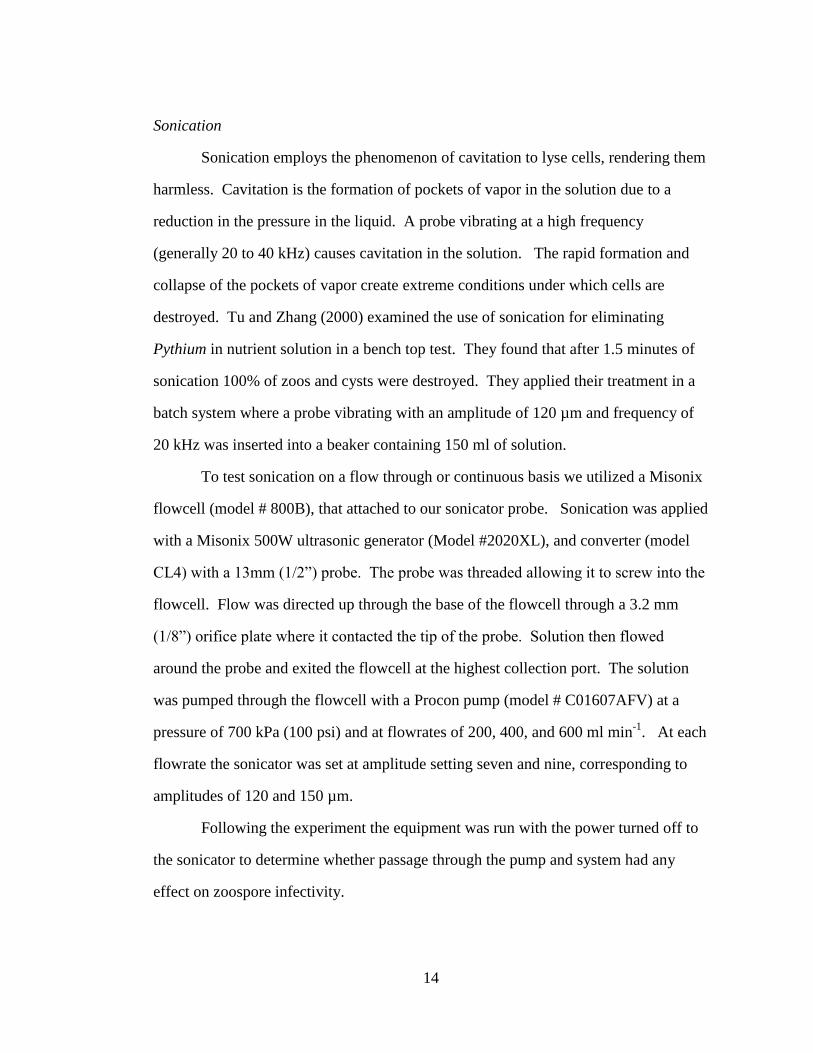
Sonication
Sonication employs the phenomenon of cavitation to lyse cells, rendering them
harmless. Cavitation is the formation of pockets of vapor in the solution due to a
reduction in the pressure in the liquid. A probe vibrating at a high frequency
(generally 20 to 40 kHz) causes cavitation in the solution. The rapid formation and
collapse of the pockets of vapor create extreme conditions under which cells are
destroyed. Tu and Zhang (2000) examined the use of sonication for eliminating
Pythium in nutrient solution in a bench top test. They found that after 1.5 minutes of
sonication 100% of zoos and cysts were destroyed. They applied their treatment in a
batch system where a probe vibrating with an amplitude of 120 µm and frequency of
20 kHz was inserted into a beaker containing 150 ml of solution.
To test sonication on a flow through or continuous basis we utilized a Misonix
flowcell (model # 800B), that attached to our sonicator probe. Sonication was applied
with a Misonix 500W ultrasonic generator (Model #2020XL), and converter (model
CL4) with a 13mm (1/2”) probe. The probe was threaded allowing it to screw into the
flowcell. Flow was directed up through the base of the flowcell through a 3.2 mm
(1/8”) orifice plate where it contacted the tip of the probe. Solution then flowed
around the probe and exited the flowcell at the highest collection port. The solution
was pumped through the flowcell with a Procon pump (model # C01607AFV) at a
pressure of 700 kPa (100 psi) and at flowrates of 200, 400, and 600 ml min-1
. At each
flowrate the sonicator was set at amplitude setting seven and nine, corresponding to
amplitudes of 120 and 150 µm.
Following the experiment the equipment was run with the power turned off to
the sonicator to determine whether passage through the pump and system had any
effect on zoospore infectivity.

15
Ultraviolet
Ultraviolet radiation is a very popular method to disinfect of recirculating
nutrient solution. Stanghellini (1984) found that a dose of 90 mJ cm-2
provided
adequate disinfestation, and Tu and Zhang (2000) found that 80 mJ cm-2
was sufficient
to kill 100% of Pythium zoos and cysts.
Ultraviolet treatment of the nutrient solution was achieved with an 8W
flowthrough ultraviolet reactor (model Aqua Ultraviolet 8W) which utilized a low
pressure bulb to produce UV-C at a wavelength of 253.7 nm. UV dosage was
regulated by varying the flowrate through the reactor. UV doses of 120 and 240 mJ
cm-2
were examined. To ensure uniform dosing of the solution, approximately 3 liters
of nutrient solution was passed through the reactor before sampling. Between runs,
the outlet of the reactor was disassembled and cleaned to prevent cross contamination.
In normal operation UV sterilization equipment requires filtration to remove
particles that prevent the transmission of the UV light. Because we were working with
new nutrient solution no such sediment was present, and so filtration was not used.
2.3 RESULTS AND DISCUSSION
2.3.1 Bioassay
To determine the level of damage associated with a particular concentration of
zoos a dilution series was conducted. Figure 2.3 illustrates the average damage visible
on the root of each plant in the bioassay. In the case of dilutions of 0 and 1 zoos ml-1
we can see that most of the damage is fairly minor, and constrained to exterior lesions
and streaking. In the 10 zoos ml-1
case we can see considerably more damage as
evidenced by the relatively large amount of dark interior streaking. Presumably the
infection has moved into the roots and advanced further than in the other two
dilutions. Low level damage in the 0 zoos ml-1
treatment was unexpected, and was

16
most likely not due to Pythium, but other organisms or mechanical damage. In a side
experiment to try and determine the cause of the damage, it was still present even after
surface sterilization of the seed with chlorine bleach.
Figure 2.3 Average root damage due to varying concentration of Pythium (Error bars
are ± 1 SE)
Because care was taken to minimize the chances of biological contamination, other
factors such as mechanical damage or a natural reaction of the root going from a
humid environment to being submerged, may have contributed to the discolorations on
the root which were then interpreted as lesions and streaking. Kinking of the roots
was observed in the 10 zoos ml-1
and to a lesser extent in the 1 zoos ml-1
dilution and
seemed to correspond with damage due to lesions. The roots of the uninfected dilution
were straight, without the abrupt directional changes visible in the more heavily
damaged roots.
0.00
1.00
2.00
3.00
4.00
5.00
6.00
7.00
8.00
9.00
0 zoospores 1 zoospore 10 zoospores
Les
ion
(#)
or
Len
gth
(m
m)
Assay Concentration (zoos ml-1)
Lesions
Streaked
Light
Dark
17
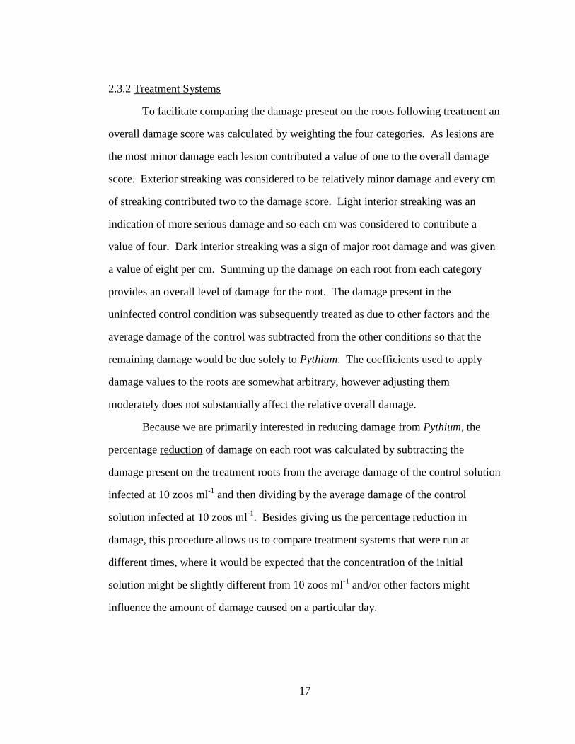
2.3.2 Treatment Systems
To facilitate comparing the damage present on the roots following treatment an
overall damage score was calculated by weighting the four categories. As lesions are
the most minor damage each lesion contributed a value of one to the overall damage
score. Exterior streaking was considered to be relatively minor damage and every cm
of streaking contributed two to the damage score. Light interior streaking was an
indication of more serious damage and so each cm was considered to contribute a
value of four. Dark interior streaking was a sign of major root damage and was given
a value of eight per cm. Summing up the damage on each root from each category
provides an overall level of damage for the root. The damage present in the
uninfected control condition was subsequently treated as due to other factors and the
average damage of the control was subtracted from the other conditions so that the
remaining damage would be due solely to Pythium. The coefficients used to apply
damage values to the roots are somewhat arbitrary, however adjusting them
moderately does not substantially affect the relative overall damage.
Because we are primarily interested in reducing damage from Pythium, the
percentage reduction of damage on each root was calculated by subtracting the
damage present on the treatment roots from the average damage of the control solution
infected at 10 zoos ml-1
and then dividing by the average damage of the control
solution infected at 10 zoos ml-1
. Besides giving us the percentage reduction in
damage, this procedure allows us to compare treatment systems that were run at
different times, where it would be expected that the concentration of the initial
solution might be slightly different from 10 zoos ml-1
and/or other factors might
influence the amount of damage caused on a particular day.

18
Electrochemical
Minute gas bubbles started to evolve from each electrode (Hydrogen gas at the
cathode and Oxygen at the anode,) when current was applied across the electrodes.
The solution in the anode compartment began to turn cloudy after a few seconds, as
the pH rose and some of the mineral salts began to precipitate out. Precipitate was not
formed in the cathode compartment. During operation of the electrochemical unit an
average 700 mA of current was drawn by the electrodes, and with a supply voltage of
100 VDC resulted in a power usage of 70 W. In the 15 minute condition the
temperature increased to approximately 35C. Figure 2.4 presents a comparison of the
percent reduction in damage at each Electrochemical duration.
Electrochemically reducing the pH and ORP does not appear to have a large
impact on Pythium, or at least at the durations we examined. This technique might be
more successful if durations were greatly increased to the order of several hours.
Current could be turned off when a target pH is achieved, and then the solution
allowed to react. However, long treatment durations would correspond to the need for
very large retention ponds making this treatment option unfeasible on a large scale.
Figure 2.4 Fraction damage reduction due to Electrochemcial Treatment
0
0.2
0.4
0.6
0.8
1
1.2
2 5 10 15
Fra
ctio
n d
am
age
red
uct
ion
Treatment time (min)

19
Pasteurization
Concentrated Pythium solution was added to preheated nutrient solution to
bring the concentration of zoos to 10 zoos ml-1
. We felt this was important because Tu
and Zhang (2000) demonstrated that Pythium can be affected at temperatures above
45C if the duration is long enough.
After addition of the Pythium concentrate and the allotted treatment time had
passed a sample was cooled using a 2 liter Erlenmeyer flask run under cold tap water.
This caused an initially rapid temperature drop, and the solutions reached ambient
temperature within 5 minutes. Figure 2.5 presents a comparison of the two treatment
temperatures and the various treatment durations at these temperatures.
Both treatment temperatures seem capable of achieving a relatively good
reduction in the level of damage. Though requiring a longer dwell time and
subsequently a larger volume in the treatment system, a temperature of 60C is easier to
attain and work with than 95C.
Figure 2.5 Fraction damage reduction due to Pasteurization
0
0.2
0.4
0.6
0.8
1
1.2
95C 15 s 95C 30 s 95C 60 s 60C 1 min 60C 2 min 60C 3 min
Fra
ctio
n d
am
age
red
uct
ion
Treatment Conditions

20
Sonication
The Misonix XL2020 used to generate the signal that causes the high
frequency vibrations in the converter can also display instantaneous power usage as a
percent of maximum. Larger amplitude corresponds to higher power consumption.
At amplitude 9 the power consumption was approximately 70% of maximum (500W)
corresponding to a value of 350 W. At amplitude 7 the power consumption was
approximately 50% or 250 W. Figure 2.6 illustrates that continuous sonication is
capable of successfully eliminating Pythium. The best results were achieved with an
amplitude of 120 µm and the lowest flowrate tested, 200 ml min-1
, though satisfactory
results were achieved with an amplitude of 150 µm. However, to deliver an effective
dose of sonic energy, our results indicate that flows greater than 200 ml min-1
are not
recommended for this size of generator.
Figure 2.6 Fraction damage reduction due to Sonication
0
0.2
0.4
0.6
0.8
1
1.2
Amp. 9
200
mL/min
Amp. 9
400
mL/min
Amp. 9
600
mL/min
Amp. 7
200
mL/min
Amp. 7
400
mL/min
Amp. 7
600
mL/min
Fra
ctio
n d
am
age
red
uct
ion
Treatment Conditions

21
Passage of Pythium containing nutrient solution through the pump and flocell
with the sonicator turned off had little effect on the damage caused by the Pythium,
indicating that any reduction in Pythium activity was due to sonication and not
pressurization and turbulence.
The stated maximum recommended flowrate for the flocell is 0.66 liters/min,
and it was developed for use with the XL2020 and other generators of a similar size.
Larger generators capable of handling greater flows exist, so scaling up the flowrate is
possible.
Ultraviolet Sterilization
Control of the flow through the UV treatment unit was with a ball valve
mounted immediately before the inlet to the reactor. Closing of the ball valve caused
more of the flow to divert through a bypass back to the reservoir containing the
Pythium infected solution. The action of the bypass also served to keep the solution
well mixed and prevented Pythium from settling on the bottom of the tank. Figure 2.7
shows the damage reduction due to UV-C doses of 120 and 240 mJ cm-2
.
Figure 2.7 Fraction reduction due to Ultraviolet Sterilization
0
0.2
0.4
0.6
0.8
1
1.2
120 240
Fra
ctio
n d
am
age
red
uct
ion
UV Dose (mJ cm-2)

22
Ultraviolet sterilization worked quite well, especially considering the energy
input was only 8 W.
2.4 CONCLUSIONS
Though the uninfected control bioassays sometimes displayed symptoms of
low levels of damage, the concept of utilizing spinach seedlings to measure Pythium
levels appears valid. Though a single bioassay is not able to provide a precise count of
the number of Pythium propagules present in a solution, when used in conjunction
with a dilution series, a reasonable estimate can be obtained. The spinach seedling
bioassay is well suited to comparing the efficacy of different treatment systems, and
whether or not they are worth developing further. The seedling bioassay has the
advantage of being very simple, which allows the testing of many conditions quickly,
without expensive or complicated laboratory procedures, or expertise requirements.
Because the ultimate goal of the research project is to develop a viable
commercial hydroponic spinach production system, testing on spinach gives a better
indication of the actual damage causing ability of the organism. Tests were performed
on the roots during the initial period where roots are most susceptible to Pythium
damage. In the production systems under evaluation the crop is floated after 48 hours
(germination time) and presumably this is when new roots would come into contact
with Pythium in the nutrient solution. The bioassays are infected at age 48 hours to
correspond to this stage.
Further refinements of the bioassay are required to better quantify how root
damage progresses. Repeated examination of the same bioassay over the course of
time following infection could provide a better picture of how lesions form, grow and
spread. This information could be used to better define the coefficients used to weight

23
the various types of damage. Additional studies could also compare the accuracy of
the bioassay with more traditional plating techniques.
The presence of damage on the roots even after the solution has undergone
treatment does not mean the crop is doomed to failure. In the short crop cycle of
spinach, Pythium may not have enough time to produce zoospores to damaging levels.
Of the new technologies tested, sonication demonstrated an ability to
successfully eliminate Pythium. Sonication in a continuous flow mode is effective
provided the flowrate doesn‟t exceed the capacity of the generator. Unfortunately the
electrochemical treatment was found to be largely ineffective at the durations we
tested. Though the system is very effective at manipulating the pH of the nutrient
solution and can achieve extreme levels, these levels don‟t appear to be extreme
enough to eliminate Pythium to a point on par with other treatment techniques.
The next step in the evaluation and selection of a treatment system for spinach
production is a comparison of the operational costs. Other factors besides energy
usage will have to be considered as well. In the case of UV sterilization, chelator
destruction, and bulb and filter replacement need to be considered. In the case of
sonication, the generator and converters are relatively expensive, and their operational
lifetime needs to be factored into the cost of operating such a system.
Another consideration is the microflora which develops in a normal nutrient
solution. Not all the microbes present are detrimental, and many can benefit the crop.
Ultraviolet sterilization tends to be more effective on smaller celled organisms which
can lead to the elimination of useful bacteria (Zhang and Tu, 2000). According to Tu
and Zhang (2000) sonication has the opposite effect and is more effective against
larger organisms. It may then be possible to target the larger zoospores and preserve
beneficial microorganisms.

24
Regardless of the technology selected, a successful spinach operation will
require diligence when it comes to monitoring the health of the crop. Perhaps a
spinach seedling bioassay will be a tool growers can utilize to ensure success.

25
CHAPTER 3: CONTINUOUS PRODUCTION EXPERIMENTS
3.1 INTRODUCTION
Pythium aphanidermatum is a water mold that can cause severe damage to
crops through destruction of their root systems. It is of particular concern in
hydroponic production systems because Pythium zoospores are mobile in water, and
can quickly spread. Pythium affects a variety of crops, but spinach has shown itself to
be particularly sensitive to this pathogen (Bates and Stanghellini, 1984). It is a leading
obstacle to the commercialization of hydroponic spinach production.
A proven technique for growing spinach hydroponically is to change out the
nutrient solution between crop cycles. This production model has been utilized in
Japan where the market for whole plant baby spinach is strong. Towards the end of
the production cycle the crop is allowed to strip the nutrients from the solution in
preparation for disposal. Careful cleaning of the growing system between crops is
then required before new nutrient solution is made up, and the new crop is installed.
Unfortunately, this model for spinach production requires the added expense of
disposing of the nutrient solution and disinfecting the growing surfaces. To allow the
re-use of the nutrient solution, considerable research has been conducted into means of
eliminating Pythium (and other nutrient solution borne pathogens). Technologies that
have proven effective have been heat (pasteurization) (Runia and Amsing, 2000),
Ultraviolet radiation (Stanghellini et al., 1984), Filtration (Tu and Harwood, 2005),
and Sonication (Tu and Zhang, 2000). These systems have proven effective and could
be implemented for a batch type production system where the nutrient solution
required to grow a crop is treated after the crop is harvested, in preparation for re-use
with the next crop. However, the use of these systems in a continuous production
(multiple stages of crop present in the same pond) floating hydroponics system has not
been presented. Pond systems have distinct advantages over other hydroponic

26
production systems including: increased reliability and performance during electrical
or other failure, easy materials handling and high space use efficiency, uniformity of
the nutrient solution, conservation of water and nutrients and the large buffering of
many parameters. It is for these reasons we have chosen to investigate means to
produce baby spinach in such a system.
As a part of her dissertation, Katzman (2003) examined the effect of Pythium
aphanidermatum concentration on damage to a spinach crop. In her system she
transplanted spinach seedlings into a pond system at day 9, and then inoculated the
pond with varying concentrations of Pythium zoospores. She then took destructive
harvests at periodic intervals and categorized damage to the roots and shoots. She
found that low levels of zoospores could be tolerated, provided the crop was harvested
early enough (typically before day 21). She suggested a hydroponic system that can
maintain a low enough concentration of zoospores in solution may be viable.
In a study of the effect of nutrient solution temperature on the spread of
Pythium, Katzman (2003) found the damage caused by the pathogen was reduced in
cooler conditions. In her study Katzman transplanted healthy 9-day-old seedlings into
ponds with temperatures of 18, 24 and 30C, and then inoculated with Pythium
zoospores. Zoospore concentrations were monitored and shoot weights were taken in
periodic harvests, until final harvest at day 28. Katzman found soon after inoculation
the concentration of zoospores in solution dropped below detection level for a period
of time, before recovering to significant concentrations. The period of time when
zoospores could not be detected in the solution was a function of temperature, with
colder solution temperatures corresponding to longer periods before re-appearance of
zoospores. The period of zoospore absence was approximately 10 days at 30C and 24
days at 18C. However, no matter the temperature, at day 28 the spinach crops

27
suffered some damage from Pythium, the higher the temperature, the more severe the
damage.
In production of baby spinach the length of time the crop spends in the ponds
is typically 14 days or less, if a consistent daily light integral of 17 mol m-2
is
maintained. In this experiment we sought to examine whether this shortened crop
cycle combined with various treatment methods to counter Pythium would allow the
continuous production of hydroponic baby spinach. The continual removal of the
source of inoculum (infected roots) before they are capable of releasing zoospores to
propagate the infection should allow such a system to work. We sought to examine
and compare two strategies to accomplish this goal. The first was to use two active
techniques (filtration and ultraviolet irradiation) to remove zoospores from the
solution and maintain a concentration acceptable to the crop. The second approach
was to use a reduced nutrient solution temperature to increase the amount of time
required by Pythium to complete its lifecycle to a period greater than the crop duration
in the pond.
3.2 METHODS AND MATERIALS
For the experiment, eight identical temperature controlled benches were
constructed (Figure 3.1). The interior dimensions of the benches were 235 cm long by
35 cm wide, and 12 cm deep. To set the depth of the nutrient solution (half-strength
Hoagland) to a height of 11 cm, a stand-pipe was used. The benches were supported
at a height of 80 cm above the level of the floor, and 150 cm below the lighting array,
which provided an average intensity of 200 µmoles m-2
s-1
PAR. Nutrient solution
from the drain cascaded into a 50 liter insulated reservoir, and through a coarse filter.
The temperature of the nutrient solution in each bench was monitored by RTD
(Omega RTD-810), and controlled through MATLAB with a USB DAQ

28
(Measurement Computing USB 1208-LS) switching an immersion heater (Aquatic
Ecosystems VT201, 200W), and a cold finger circulating chilled water. The nutrient
solution was pumped up to the bench by positive displacement pumps (Little Giant 2-
MCHD).
Figure 3.1 Overview photograph of spinach growing benches used in the multi-cohort
evaluation of filtration, UV sterilization and temperatures suppression in continuous
production.
Intact spinach seed (cv. Eagle was seeded into Rediearth® growing medium,
corrected to a moisture content of 3.0 to 1.0, in 132 cell styrofoam plug trays of area c.
0.1 m2 (Beaver Plastic, modified 288 cell flats). Once seeded and covered, the trays
were placed in darkness in a growth chamber set at 26C, to germinate for 48 hours.
Following 24 hours in the growth chamber c. 100 µmol m-2
s-1
of continuous light was
provided on to the emerging seedlings to prevent stretching. At the time of flotation,
trays were placed in the growing bench at the end closest to the inflow of nutrient
solution from the pump. Space for the new float was made by pushing the existing
floats towards the drain of the bench. To provide a consistent plant density, floats

29
were randomly thinned to a final count of 72 plants because germination percentage
was variable and only about 70%. Target daily light integral was set for 17 mol m-2
d-
1, and the day/night temperature was set at 23C. pH and EC were monitored daily and
adjusted to targets of 5.8, and 1400 mS cm-1
, respectively when necessary. To
maintain a constant system volume, the reservoir was replenished daily with modified
half strength Hoaglands solution. Solution flow rate was balanced across all benches,
and set to produce an average velocity of 1 cm s-1
under the floats.
Three treatment methods, filtration, ultraviolet and temperature reduction were
examined, and each had an inoculated, and un-inoculated condition requiring a total of
six separate production systems or benches. An additional two benches were
maintained at 27.5C with and without inoculation, and served as controls for all three
of the treatment methods. The filtration system was installed inline after the pump and
consisted of two 25.4 cm (10") opaque polypropylene filter units (Cole-Parmer
C29820-32). The first filter provided filtration to a level of 5 microns (Cole Parmer
C-01509-15), and the second to a level of 1 micron (Cole Parmer C-01509-14).
Ultraviolet treatment was provided by Aqua ultraviolet aquarium treatment units
(Aqua Ultraviolet Classic 8), and provided a dose of UV equivalent to 100 mJ cm-2
.
To prepare for the experiment, crops in all benches were grown at 27.5C. New
flats were added to the bench every three days, until a full cohort of 5 flats was in the
system. At that time enough Pythium zoospores were placed into the systems to be
inoculated, to bring the concentration to a level of 100 zoospores ml-1
(c. 7 million
zoospores per bench). Bioassays utilizing spinach seedlings were prepared beforehand
and samples from the growing bench and reservoir were taken 15 minutes after
inoculation and applied to the bioassays. The subsequent damage to the bioassays
indicated Pythium had successfully spread throughout the system. The production
systems were allowed to run as usual for 24 hours, without application of remedial
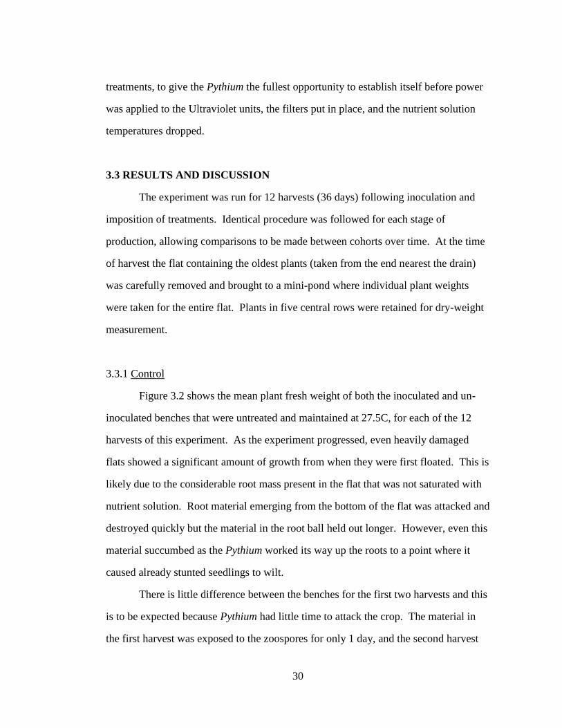
30
treatments, to give the Pythium the fullest opportunity to establish itself before power
was applied to the Ultraviolet units, the filters put in place, and the nutrient solution
temperatures dropped.
3.3 RESULTS AND DISCUSSION
The experiment was run for 12 harvests (36 days) following inoculation and
imposition of treatments. Identical procedure was followed for each stage of
production, allowing comparisons to be made between cohorts over time. At the time
of harvest the flat containing the oldest plants (taken from the end nearest the drain)
was carefully removed and brought to a mini-pond where individual plant weights
were taken for the entire flat. Plants in five central rows were retained for dry-weight
measurement.
3.3.1 Control
Figure 3.2 shows the mean plant fresh weight of both the inoculated and un-
inoculated benches that were untreated and maintained at 27.5C, for each of the 12
harvests of this experiment. As the experiment progressed, even heavily damaged
flats showed a significant amount of growth from when they were first floated. This is
likely due to the considerable root mass present in the flat that was not saturated with
nutrient solution. Root material emerging from the bottom of the flat was attacked and
destroyed quickly but the material in the root ball held out longer. However, even this
material succumbed as the Pythium worked its way up the roots to a point where it
caused already stunted seedlings to wilt.
There is little difference between the benches for the first two harvests and this
is to be expected because Pythium had little time to attack the crop. The material in
the first harvest was exposed to the zoospores for only 1 day, and the second harvest

31
for 4 days. At this point these flats had well established root systems and considerable
shoot mass. By the third harvest the difference was more pronounced and at the fourth
harvest dramatically different. Though the subsequent flats suffered extreme root
damage, enough material was present to continue the infection. Figure 3.3 shows the
difference in root appearance between the healthy and infected flats.
Figure 3.2 Average plant fresh weights at time of harvest in control benches
Figure 3.3 Roots of uninfected (left) and infected (right) flats
0.00
1.00
2.00
3.00
4.00
5.00
6.00
7.00
0 2 4 6 8 10 12
Harv
est
Fre
sh M
ass
(g p
lan
t-1)
Harvest Number
B4 (inoculated) B6 (control)

32
3.3.2 Filtration
Figure 3.4 shows the mean plant fresh weight for the filtration systems. As in
the case of the inoculated control bench damage at harvest 4 was severe. In
subsequent harvests it appeared that the filtration system was allowing the infected
bench to recover, but at harvest 8 the infection was able to reassert itself. It appears
the filtration system was effective in removing free zoospores from the solution,
however, not to a level that is tolerable by the crop.
Figure 3.4 Average plant fresh weight in the filtration, control (uninoculated) and
inoculated systems, at time of harvest.
To improve the chances for active disinfection to succeed, a smaller volume of
nutrient solution was used per plant than would be found in a typical pond system. A
smaller volume was used, to decrease the turnover time of the pond, and to attempt to
get directional bulk flow from the inlet to the outlet. It was thought that creating a
velocity gradient would limit the migration of zoospores upstream towards the
younger, more vulnerable plants. This also caused the roots to arrange themselves in
the direction of flow which allowed the roots on the edge of a younger cohort to come
into contact with older cohort root material. However, infection was not limited to
0.00
1.00
2.00
3.00
4.00
5.00
6.00
0 2 4 6 8 10 12Harv
est
Fre
sh M
ass
(g p
lan
t-1)
Harvest Number
B1 (inoculated) B8 (control)

33
edge plants alone indicating zoospores were able to migrate upstream. This is not
surprising as the flow velocity immediately beneath the floats was likely low enough
to allow Pythium migration.
3.3.3 Ultraviolet Irradiation
Figure 3.5 shows the results of the ultraviolet irradiation systems. As in the
case of filtration, the UV system was not able to prevent the Pythium infection from
propagating. Again there appeared to be an initial recovery (even better than that
observed with filtration) followed by a relapse. In addition, the control bench which
was subjected to UV treatment but without inoculation also fared poorly. During this
time, leaves gradually became pale yellow-green in color and failed to grow as well as
the other benches. Ultraviolet radiation has been shown to destroy the chelator
responsible for keeping iron soluble in a hydroponic solutions (Acher et al., 1997).
Though new nutrient solution containing the complete mix of required elements was
added daily through topping up of the reservoirs, iron content of the solution dropped
to zero, and it is likely that the crop suffered from iron chlorosis.
Figure 3.5 Average plant fresh weight in the Ultraviolet systems at time of harvest
0.00
1.00
2.00
3.00
4.00
5.00
6.00
7.00
0 2 4 6 8 10 12Harv
est
Fre
sh M
ass
(g p
lan
t-1)
Harvest Number
B2 (inoculated) B7 (control)

34
3.3.4 Root zone temperature depression
Of the treatment systems tested, temperature depression appeared to perform
the best, as can be seen in Figure 3.6. The initial dosage of Pythium was enough to
cause considerable damage to the crop, and we see this in reduced fresh weights in the
fourth and fifth harvests. The harvest from the fifth cohort suffered the most damage
which is to be expected, as it was the youngest material present at the time of infection
and the zoospores added to the solution obviously set it back. However, the infection
did not propagate and it seems damage was limited only to those plants directly
exposed to the initial infection. Visual inspection of roots showed it took several
additional harvests before all traces of root disease disappeared, but the remnant
infection was so slight it did not manifest itself in shoot biomass reduction.
In comparing the average plant fresh weights among the controls it is apparent
spinach performed better under cooler root conditions. A steady increase in average
plant fresh weight until harvest 6 is apparent. This is to be expected as the crops spent
more and more time under the more favorable temperature condition until harvest 6, at
which point the entire crop cycle was at a root zone temperature of 20C.
Figure 3.6 Average Plant fresh weight in the temperature depression systems at
harvest.
0.00
1.00
2.00
3.00
4.00
5.00
6.00
7.00
8.00
9.00
0 2 4 6 8 10 12
Harv
est
Fre
sh M
ass
(g p
lan
t-1)
Harvest NumberB5 (inoculated) B3 (control)

35
3.4 CONCLUSIONS
Though it initially appeared active disinfection through filtration and
ultraviolet irradiation would prove a viable means of suppressing Pythium for
continuous pond culture, each of these systems was unable to eliminate the infection.
It was clear they were having some positive effect as the crops in the inoculated
control (no treatment) bench generally did not perform as well. However, the effect
was not great enough to eliminate the infection or to be commercially useful.
Temperature depression appeared to work very well. We believe 20C was low
enough a temperature to slow the reproductive cycle of Pythium to a point where it
could not reproduce before the source of inoculum for the next generation was
removed.
While temperature depression worked very well in eliminating the effects of a
heavy infection of a virulent strain of Pythium aphanidermatum, there is no guarantee
that more virulent and/or rapidly reproducing strains of P. aphanidermatum do not
exist for which the method will not work. If such strains should be encountered, one
recourse would be to use a yet lower solution temperature and shorter crop cycle.
Other species of Pythium such as Pythium disoticum have temperature optima lower
than Pythium aphanidermatum and could potentially thrive at 20C (Bates and
Stanghellini, 1984), though Katzman (2003) was not able to isolate that species in
nutrient solution taken from a commercial scale lettuce production system, located in
Ithaca, NY.

36
CHAPTER 4: GREENHOUSE TEMPERATURE SIMULATION MODEL
4.1 INTRODUCTION:
In Katzman‟s dissertation (Katzman 2003) and subsequent Pythium studies
(Albright et al., 2007), the central role of nutrient solution temperature on the
reproduction and spread of Pythium was identified. Before evaluating the
performance of hydroponic babyleaf spinach production techniques in a commercial
setting, a means of predicting the nutrient solution temperature in a greenhouse as a
function of climate is required. In addition, because it is assumed that production will
occur in a modern greenhouse with cooling and heating systems, supplemental lights
and shade, the greenhouse simulation model must take into account the technologies
available to a grower to optimize the growing environment, and the effects of these
systems on the plant environment.
Many greenhouse models have been developed, including ones that
incorporate shading systems; however, most models stop at either the crop canopy or
the ground surface temperature. In the hydroponic babyleaf spinach system developed
at Cornell, individual spinach plants are grown in Speedling type trays filled with a
peatlite mixture. These styrofoam trays are then “floated” in a nutrient solution pond
typically 20 to 30 cm deep. A similar system is used commercially to produce
hydroponic lettuce; however, rather than use the densely packed speedling trays, the
individual lettuce plants are spaced (and respaced depending on their stage of growth)
on 2.5 cm (1”) thick styrofoam boards. The need to model nutrient solution
temperature as a function of climate is highlighted by the need to control the solution
temperature in lettuce production ponds, even though this crop is less susceptible to
Pythium than spinach. In the summer months pond temperatures can increase up to
30C if left uncooled; a temperature that would quickly lead to the rapid spread of
Pythium and extreme damage to spinach production.

37
In one of the first forays into studying the commercial production of
hydroponic spinach, Bates and Stanghellini (1984) identified seasonal effects of
Pythium outbreaks in their greenhouse in Arizona. With a range of pond temperatures
from 17 to 27C they found the dominant species of Pythium changed over the course
of the year. Above 23C, Pythium aphanidermatum was the predominant species, and
below 23C, Pythium disoticum dominated. In her dissertation, Katzman (2003) found
that maintaining a nutrient solution of 18C slowed the development of Pythium
aphanidermatum when she inoculated her spinach crops. In the NYSERDA spinach
disease project (Albright 2007), temperatures of 20C were found to prevent the spread
of Pythium infection from cohort to cohort grown in the same pond, by effectively
breaking the reproductive cycle of Pythium through the removal of infected roots
before they had the opportunity to release zoospores.
The key to successfully overcoming Pythium aphanidermatum in hydroponics
is to reduce the nutrient solution temperature to the point where the growth and
maturation rate of Pythium is slowed enough so the crop can complete its growth
cycle, and to harvest before infection has a chance to spread. The modeling of the
growth cycle of spinach is equally as important as the temperature of the nutrient
solution. The growth cycle of spinach is essentially controlled by the amount of light
that the crop receives. In the winter months in Ithaca, NY, natural sunlight is not
adequate to produce a harvestable baby spinach crop in two weeks, whereas, in
summer months, it may take considerably less time. To balance the production over
the course of the year, supplemental lighting and shading is used. Lighting and
shading not only have an important influence on the growth of the crop, they also
significantly affect the thermal environment of the greenhouse. Supplemental lights
are not 100% efficient and produce considerable amounts of heat as well. Shading
systems not only block a portion of the light, they also essentially create two airspaces

38
within the greenhouse that can have quite different temperatures. Shading also
reduces radiative heat loss during the night and can help insulate the greenhouse.
Because of the important role these two controls have on both the greenhouse
environment, and crop production, they were included in the greenhouse model.
The greenhouse model provides the input needed by the subsequent spinach
growth and Pythium disease models. The greenhouse model provides temperatures
and light levels (and light source) to the spinach growth model, which allows the
prediction of how a spinach crop will develop. Nutrient solution temperatures and the
status of the spinach crop from the spinach growth model are the input to the Pythium
disease model.
The basis of the Pythium aphanidermatum simulation is the temperature of the
nutrient solution and so the need for a model that will provide not only these values,
but the lighting environment that leads to them.
Objectives:
1. to develop a greenhouse climate simulation model capable of predicting
nutrient solution pond temperatures under standard controlled environment
agriculture operating principles,
2. to validate the operation of the model with both simulated and real weather
data.
4.2 LITERATURE REVIEW:
Greenhouse simulation models are usually developed for a specific purpose
including control and production/operation optimization. Models are also used to
better understand the complex interactions that occur within greenhouses, and to
evaluate new crops, or ways of managing them (Jones et al., 1995). With the
increasing ease and power of computer simulations, greenhouse models have become

39
very popular with researchers. One of the most referenced is by Bot (1983). In this
work, Bot quantifies the fundamental physical processes at work within a greenhouse,
focusing on ventilation, radiation and convective exchanges. In Bot‟s model, thermal
and moisture interactions with the plant canopy and underlying soil are included.
A primary focus in greenhouse models is the temperature of the air within.
Whether it is estimating the effect of a night curtain (Chandra and Albright, 1980), or
intermittent fogging (Abdel-Ghany and Kozai, 2005), modelers are usually interested
in the aerial temperature of the greenhouse. One of the main reasons for using a
greenhouse is to moderate the temperature, making the conditions more conducive to
plant growth. However, few models include the temperature of the nutrient solution in
which a floating hydroponic crop is grown. This omission is likely because relatively
few greenhouse crops (other than leafy greens) are grown in this fashion. Also the
nutrient solution temperature may often be ignored as a simplification because, as a
general rule, the nutrient solution tends to follow longer term aerial temperature
trends. Usually, only when the nutrient solution temperature is a primary concern of
the model, is it included. Such a case is outlined in Zhu et al. (1998) where
greenhouses were used to cover aquaculture ponds, within which the temperature of
water has powerful effects not only on the growth and development of the fish, but
also on the solubility (and availability) of dissolved oxygen.
Though Bot included interactions with the plant canopy, crop response to the
greenhouse climate was not a goal of the work. In other models however, crop
response is a fundamental component. In the HORTISIM model Gijzen et al. (1998),
developed a model encompassing seven submodels including: weather, greenhouse
climate, crop, soil, greenhouse manager, crop manager and soil manager. The
HORTISIM model is used for predicting both the production of tomatoes and sweet
peppers, and the cost of that production in terms of energy, CO2 and water in quite

40
different climactic locations (data from the Netherlands and Israel was used to validate
the model). Not all models need to be so complex, and often assumptions can be
made to simplify both the form of the model, and the computational requirements.
4.3 METHODS AND MATERIALS:
4.3.1 Model Formulation:
To model temperature and moisture relations in a greenhouse, one approach is
to divide the greenhouse into several layers. Assuming that there is adequate
mixing/thermal conductivity, temperatures within each layer are considered to be
uniform. Assuming uniform temperatures and properties within layers is called a
lumped parameter approach. This approach was used to model heat flow through the
layers of a green roof (Lambert 2006). Temperature changes within layers are due to
conduction, convection, radiation and enthalpy exchanges, depending on the medium
of which the layer is made and the layer with which it is exchanging energy. To
determine the change in temperature of the different layers over time, the heat lost
from a particular layer is subtracted from the heat input to that same layer and the
difference is the storage. Dividing by the heat capacitance of the layer medium gives
the change in temperature.
To account for climate seasonal and diurnal changes it is necessary to model
how the greenhouse layers change temperature over time. The assumption is that
temperatures within each layer are constant and uniform over the course of a set time
step. A time step of one hour was selected as this is less than the period of diurnal
change and greater than the thermal response time of a greenhouse. Climatic data is
usually available on an hourly basis, and more important, an hour is usually
sufficiently long for adequate convection and conduction to take place to ensure
temperatures are relatively uniform within layers. Another reason for an hourly time

41
step is many greenhouse operational decisions are made on an hourly basis
(temperature setpoints, lighting). This type of model is called a stepwise steady state
model. Stepwise describes the time steps used, and steady state for the assumption
that temperatures are uniform and constant within layers for the duration of each time
step.
Another major simplifying assumption is that energy flows within the
greenhouse are one dimensional and that energy exchange through the sides of the
greenhouse is negligible, compared to magnitudes of other flows.
With the exception of radiation, the other heat fluxes, conduction, convection
and exchange of air of differing enthalpies, can all be described by linear equations.
The Stephan-Boltzman Law governs the exchange of energy between two surfaces at
temperatures T1 and T2, through radiation:
𝑟𝑎𝑑𝑖𝑎𝑡𝑖𝑣𝑒 𝑓𝑙𝑢𝑥 = 휀𝜍𝐴 𝑇14 − 𝑇2
4
4.1
where: ε is the emissivity of the material
ζ is the Stephan-Boltzman constant
A is the surface area
This relation is not linear, but it can be linearized if the assumption is made that the
temperature differences are not large, and do not change drastically between time steps
(equation 4.2).
𝑟𝑎𝑑𝑖𝑎𝑡𝑖𝑣𝑒 𝑓𝑙𝑢𝑥 ≅ 휀𝜍𝐴 𝑇1,𝑡−1 + 𝑇2,𝑡−1
2
3
𝑇1 − 𝑇2
4.2
Using this simplification it is possible to develop a series of linear equations that
describe the flow of energy between the layers which can then be solved
simultaneously to give the temperature of each layer.
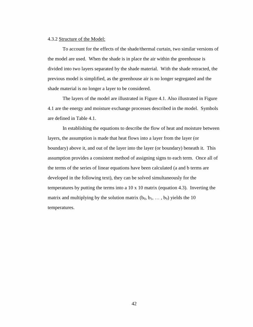
42
4.3.2 Structure of the Model:
To account for the effects of the shade/thermal curtain, two similar versions of
the model are used. When the shade is in place the air within the greenhouse is
divided into two layers separated by the shade material. With the shade retracted, the
previous model is simplified, as the greenhouse air is no longer segregated and the
shade material is no longer a layer to be considered.
The layers of the model are illustrated in Figure 4.1. Also illustrated in Figure
4.1 are the energy and moisture exchange processes described in the model. Symbols
are defined in Table 4.1.
In establishing the equations to describe the flow of heat and moisture between
layers, the assumption is made that heat flows into a layer from the layer (or
boundary) above it, and out of the layer into the layer (or boundary) beneath it. This
assumption provides a consistent method of assigning signs to each term. Once all of
the terms of the series of linear equations have been calculated (a and b terms are
developed in the following text), they can be solved simultaneously for the
temperatures by putting the terms into a 10 x 10 matrix (equation 4.3). Inverting the
matrix and multiplying by the solution matrix (b0, b1, … , b9) yields the 10
temperatures.

43
Figure 4.1 Diagram of thermal layers and energy flow processes within the
greenhouse model (F. John Peters).

44
a00 a01 0 0 0 0 0 0 0 0
a10 a11 a12 0 0 0 0 0 0 0
0 a21 a22 a23 0 0 0 0 0 0
0 0 a32 a33 a34 0 0 0 0 0
0 0 0 a43 a44 a45 a46 a47 0 0 x
0 0 0 0 a54 a55 a56 a57 0 0
0 0 0 0 a64 a65 a66 a67 a68 0
0 0 0 0 a74 a75 a76 a77 a78 a79
0 0 0 0 0 0 a86 a87 a88 a89
0 0 0 0 0 0 0 a97 a98 a99
Tsoil
b0 Tconcrete
b1 Twater
b2 Tmedium
b3 Tsurface = b4 Tcanopy
b5 Tair1
b6 Tshade
b7 Tair2
b8 Tglass
b9
4.3
An additional component to the flow of energy necessary when modeling air
layers is the enthalpy, which is a function of not only the temperature of the air, but
the amount of moisture within the air. The enthalpy of air is defined in equation 4.4.
= 1006𝑡 +𝑊 2501000 + 1805𝑡 4.4
where: h is the enthalpy of the moist air (J kg-1
)
1006 is the specific heat of dry air (J kg-1
K-1
)
t is the temperature in Celsius (C)
W is the humidity ratio (kg water kg-1
dry air)
2501E3 is the Heat of Vaporization at 0 C(J kg-1
)
1805 is the specific heat of water vapor (J kg-1
K-1
)

45
When considering the case of bulk exchanges of air through venting and
infiltration, it is assumed (for the purposes of developing the equations of the model)
that energy flows into the layer from the source of the flow (whether that is ambient
air or another air space) and that energy, in an identical mass of air, leaves the layer
(the volume of air in the layer remains constant though the energy content of the air
changes). It is necessary to mix the existing mass of air with the incoming mass to
determine the values of its properties. Assuming one mass of air with enthalpy h1,
humidity ratio W1 and volume V1 mixes with a second mass of air with enthalpy h2,
humidity ratio W2 and volume V2, the resultant air mass properties are defined in
equations 4.5 and 4.6;
3 =
1𝑉1𝑉𝑠𝑎1
+ 2𝑉2𝑉𝑠𝑎2
𝑉1𝑉𝑠𝑎1
+𝑉2𝑉𝑠𝑎2
4.5
where: Vsa1 is the air specific volume of air volume 1 (m3 kg
-1 dry air)
Vsa2 is the air specific volume of air volume 2 (m3 kg
-1 dry air)
𝑊3 =
𝑊1𝑉1𝑉𝑠𝑎1
+𝑊2𝑉2𝑉𝑠𝑎2
𝑉1𝑉𝑠𝑎1
+𝑉2𝑉𝑠𝑎2
4.6
Table 4.1 summarizes the variables and parameters used in the energy and
moisture flow equations, and gives their symbols and assumed values. Parameter
values were estimated or developed from data given in heat and mass transfer texts
and ASHRAE (American Society of Heating, Refrigerating and Air-Conditioning
Engineers) (2009) and ASABE (American Society of Agricultural and Biological
Engineers) (2007) standards.
46
Table 4.1 Symbols, definition and values of parameters and variables used in
developing the energy flow equations of the lumped parameter stepwise steady state
greenhouse simulation model.

47
αcrop Long Wave radiation Absorbance of the crop (unitless) 0.95
αmedium Long Wave radiation Absorbance of the medium (unitless) 0.9
αshade Long Wave radiation Absorbance of the shade (unitless) 0.5
Δ Slope of the vapor pressure curve (kPa K-1
) variable
εcrop Long Wave Emissivity of the crop (unitless) 0.95
εmedium Long Wave Emissivity of the medium (unitless) 0.95
εshade Long Wave Emissivity of the shade (unitless) 0.5
εglass Long Wave Emissivity of the glass (unitless) 0.95
γ Psychrometric constant (kPa K-1
) variable
ρconcrete Density of concrete (kg m-3
) 2200
ρcrop Canopy reflectivity to solar and supplemental light (unitless) 0.25
ρglass Glass reflectivity to solar radiation (unitless) 0.25
ρmedium Density of root medium (kg m-3
) 100
ρsoil Density of soil (kg m-3
) 1800
ρwater Density of nutrient solution (kg m-3
) 1000
ϕl Radiation from supplemental lights, (J m-2
hr-1
) variable
ϕsolar,glass Solar radiation through the glass (ϕsolar,outsideηglass), (J m-2
hr-1
) variable
ϕsolar,outside Solar radiation outside the greenhouse glass, (J m-2
hr-1
) variable
ϕsolar,shade Solar radiation through the shade (ϕsolar,glassηshade), (J m-2
hr-1
) variable
ηglass Transmittance of the greenhouse glass to solar radiation
(unitless) 0.7
ηshade Transmittance of the shade to solar radiation (unitless) 0.3
A Area of greenhouse (m2) 10000

48
Table 4.1 (Continued)
cpsoil Heat capacity of soil (J kg-1
K-1
) 1217
cpconcrete Heat capacity of concrete (J kg-1
K-1
) 882
cpwater Heat capacity of nutrient solution (J kg-1
K-1
) 4184
cpmedium Heat capacity of medium (including Styrofoam float) (J kg
-
1K
-1)
840
(ea-ed) Vapor pressure deficit (kPa) variable
ET Crop Evapotranspiration (J m-2
hr-1
) variable
ETo Reference Crop Evapotranspiratioin (mm hr-1
) variable
G Soil heat flux, (MJ m-2
h-1
) variable
hcrop-air Convective heat transfer coefficient between crop and
greenhouse air (J m-2
hr-1
K-1
) 29000
hglass-air Convective heat transfer coefficient between glass and
greenhouse air (J m-2
hr-1
K-1
) 29000
hglass-
ambient
Convective heat transfer coefficient between glass and
ambient air (J m-2
hr-1
K-1
) 35000
hglass-air2 Convective heat transfer coefficient between glass and
greenhouse airspace 2 (J m-2
hr-1
K-1
) 29000
hmedium-air Convective heat transfer coefficient between medium surface
and greenhouse air (J m-2
hr-1
K-1
) 29000
hshade-air1 Convective heat transfer coefficient between shade and
greenhouse airspace 1 (J m-2
hr-1
K-1
) 29000
hshade-air2 Convective heat transfer coefficient between shade and
greenhouse airspace 2 (J m-2
hr-1
K-1
) 29000
hwater
Convective heat transfer coefficient between concrete and
nutrient solution, and the nutrient solution and medium (J m-2
hr-1
K-1
)
42000
Hfg Heat of vaporization (kJ kg-1
) variable

49
Table 4.1 (Continued)
K Canopy extinction coefficient (unitless) 0.74
LAI Leaf Area Index (m
2 leaf area m
-2 ground surface area for
plant canopy) 0.7
ksoil Thermal conductivity of soil (J m-1
hr-1
K-1
) 6480
kconcrete Thermal conductivity of concrete (J m-1
hr-1
K-1
) 4608
kmedium Thermal conductivity of medium (J m-1
hr-1
K-1
) 700
Kc Crop coefficient to convert reference ET to spinach ET
(unitless) 1.84
n1 Air exchanged with the outside due to infiltration (m
3 m
-2 hr
-
1)
4
nv1-v2 Volume of air exchanged between airspace 1 and 2(m3m
-2hr
-1) 2
𝑞 𝑒𝑎𝑡𝑒𝑟 Heat input to the greenhouse air due to heating system (J m
-2
hr-1
) 1.33E6
𝑞 𝑙𝑎𝑚𝑝𝑠 Heat input to the greenhouse air due to supplemental lights (J
m-2
hr-1
) 5.96E5
𝑞 𝑝𝑢𝑚𝑝 Heat input to the nutrient solution by the pump (J m-2
hr-1
) 6770
Rn Net radiation at the crop surface (MJ m-2
h-1
) variable
Tair Temperature of the greenhouse air (K) variable
Tair, t-1 Temperature of the greenhouse air in the previous hour (K) variable
Tair1 Temperature of the greenhouse air in airspace 1 (K) variable
Tair1, t-1 Temperature of the greenhouse air in airspace 1 in the
previous hour (K) variable
Tair2 Temperature of the greenhouse air in airspace 2 (K) variable
Tair2, t-1 Temperature of the greenhouse air in airspace 2 in the
previous hour (K) variable
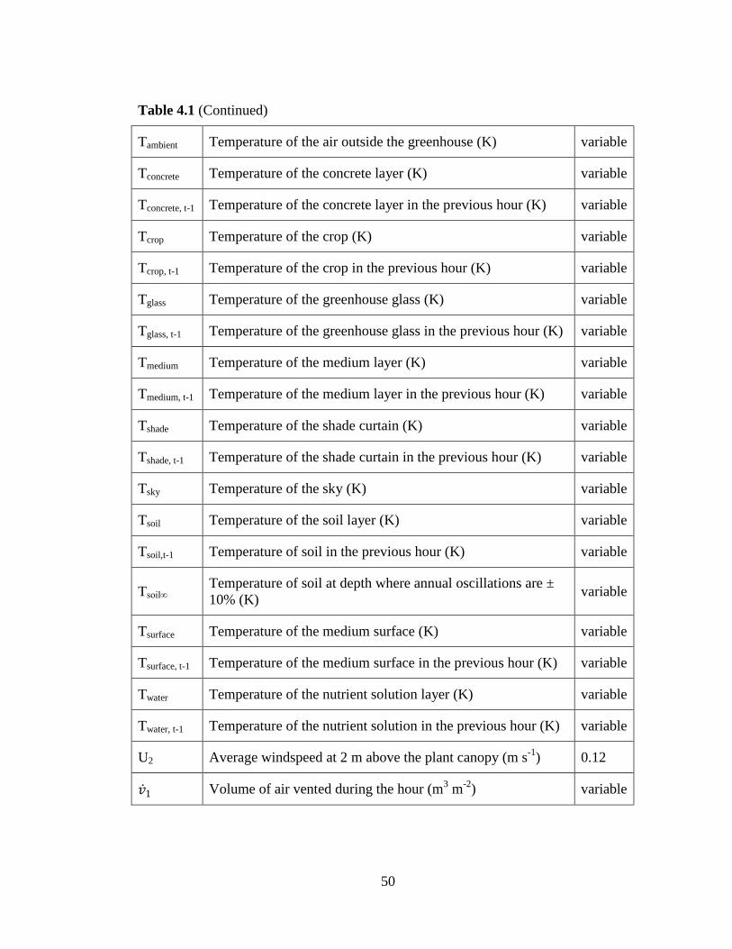
50
Table 4.1 (Continued)
Tambient Temperature of the air outside the greenhouse (K) variable
Tconcrete Temperature of the concrete layer (K) variable
Tconcrete, t-1 Temperature of the concrete layer in the previous hour (K) variable
Tcrop Temperature of the crop (K) variable
Tcrop, t-1 Temperature of the crop in the previous hour (K) variable
Tglass Temperature of the greenhouse glass (K) variable
Tglass, t-1 Temperature of the greenhouse glass in the previous hour (K) variable
Tmedium Temperature of the medium layer (K) variable
Tmedium, t-1 Temperature of the medium layer in the previous hour (K) variable
Tshade Temperature of the shade curtain (K) variable
Tshade, t-1 Temperature of the shade curtain in the previous hour (K) variable
Tsky Temperature of the sky (K) variable
Tsoil Temperature of the soil layer (K) variable
Tsoil,t-1 Temperature of soil in the previous hour (K) variable
Tsoil∞ Temperature of soil at depth where annual oscillations are ±
10% (K) variable
Tsurface Temperature of the medium surface (K) variable
Tsurface, t-1 Temperature of the medium surface in the previous hour (K) variable
Twater Temperature of the nutrient solution layer (K) variable
Twater, t-1 Temperature of the nutrient solution in the previous hour (K) variable
U2 Average windspeed at 2 m above the plant canopy (m s-1
) 0.12
𝑣 1 Volume of air vented during the hour (m3 m
-2) variable

51
Table 4.1 (Continued)
V Volume of air in greenhouse (m3 m
-2) 4
V1 Volume of air in greenhouse airspace 1 (m3 m
-2) 3
V2 Volume of air in greenhouse airspace 2 (m3 m
-2) 1
Vsaair Specific volume of greenhouse air (m3 kg
-1) variable
Vsaair1 Specific volume of greenhouse air in airspace 1 (m3 kg
-1) variable
Vsaair2 Specific volume of greenhouse air in airspace 2 (m3 kg
-1) variable
Vsaamb Specific volume of the outside air (m3 kg
-1) variable
Vsavent Specific volume of the vent air (m3 kg
-1) variable
Wair Humidity ratio of the greenhouse air (kg water kg-1
dry air) variable
Wair1 Humidity ratio of the greenhouse air in airspace 1 (kg water
kg-1
dry air) variable
Wair2 Humidity ratio of the greenhouse air in airspace 2 (kg water
kg-1
dry air) variable
Wamb Humidity ratio of the outside air (kg water kg-1
dry air) variable
Wvent Humidity ratio of the vent air (kg water kg-1
dry air) variable
zair Thickness of air level (medium to outer glass) (m) 4.0
zair1 Thickness of air level below shade (m) 3.0
zair2 Thickness of air level above shade (m) 1.0
zconcrete Thickness of concrete layer (m) 0.15
zmedium Thickness of medium layer (m) 0.05
zsoil Thickness of soil layer (m) 6.1
zwater Thickness (depth) of nutrient solution layer (m) 0.3

52
Greenhouse Model with shading
Soil Layer:
The first layer is the soil beneath the greenhouse structure. It is bounded by
the deep soil, and the concrete that forms the floor of the greenhouse. The thickness
of this layer was determined by assuming the thermal properties of the soil, and
determining the depth at which the yearly temperature swings would dampen to 10%
of the surface value. To estimate this depth we can use the relation from Carslaw and
Jaeger (1959):
𝑎𝑚𝑝𝑙𝑖𝑡𝑢𝑑𝑒 𝑜𝑓 𝑡𝑒𝑚𝑝𝑒𝑟𝑎𝑡𝑢𝑟𝑒 𝑜𝑠𝑐𝑖𝑙𝑙𝑎𝑡𝑖𝑜𝑛 = 𝑒−𝑥
𝜔2𝑘
4.7
where: x is the depth (m)
ω is the frequency of oscillation (s-1
) 3.17E-08 (1 year)
k is the thermal diffusivity of the soil (m2 s
-1) 1.14E-07
It is assumed that energy flows into and out of this layer through conduction. The flux
of energy into the soil is described in equation 4.8, the flux out, in equation 4.9, and
the storage in equation 4.10.
𝑓𝑙𝑢𝑥 𝑖𝑛 = 𝐴
1𝑧𝑠𝑜𝑖𝑙𝑘𝑠𝑜𝑖𝑙
+𝑧𝑐𝑜𝑛𝑐𝑟𝑒𝑡𝑒𝑘𝑐𝑜𝑛𝑐𝑟𝑒𝑡𝑒
𝑇𝑐𝑜𝑛𝑐𝑟𝑒𝑡𝑒 − 𝑇𝑠𝑜𝑖𝑙
4.8
𝑓𝑙𝑢𝑥 𝑜𝑢𝑡 = 𝐴
𝑘𝑠𝑜𝑖𝑙𝑧𝑠𝑜𝑖𝑙
2
𝑇𝑠𝑜𝑖𝑙 − 𝑇𝑠𝑜𝑖𝑙∞
4.9
𝑠𝑡𝑜𝑟𝑎𝑔𝑒 = 𝐴 𝜌𝑠𝑜𝑖𝑙 𝑐𝑝𝑠𝑜𝑖𝑙 𝑧𝑠𝑜𝑖𝑙 𝑇𝑠𝑜𝑖𝑙 − 𝑇𝑠𝑜𝑖𝑙 𝑡−1
4.10
Putting these equations together and solving for the coefficients of each temperature
term results in equations 4.11 and 4.12.
𝑎00 = 𝐴 𝑘𝑠𝑜𝑖𝑙𝑧𝑠𝑜𝑖𝑙
𝑇𝑐𝑜𝑛𝑐𝑟𝑒𝑡𝑒 4.11

53
𝑎01 = −1 𝐴
𝑘𝑠𝑜𝑖𝑙𝑧𝑠𝑜𝑖𝑙
+𝑘𝑠𝑜𝑖𝑙𝑧𝑠𝑜𝑖𝑙
2
+ 𝜌𝑠𝑜𝑖𝑙 𝑐𝑝𝑠𝑜𝑖𝑙 𝑧𝑠𝑜𝑖𝑙 𝑇𝑠𝑜𝑖𝑙
4.12
The constant is given in equation 4.13.
𝑏0 = 𝐴 𝑘𝑠𝑜𝑖𝑙𝑧𝑠𝑜𝑖𝑙
2
𝑇𝑠𝑜𝑖𝑙∞ + 𝐴𝜌𝑠𝑜𝑖𝑙 𝑐𝑝𝑠𝑜𝑖𝑙 𝑧𝑠𝑜𝑖𝑙𝑇𝑠𝑜𝑖𝑙 𝑡−1
4.13
Concrete Layer:
The second layer is that of the concrete foundation or base of the pond. This
layer is bounded below by the soil beneath the greenhouse, and above by the pond
nutrient solution.
Energy is exchanged with the ground layer through conduction, whereas
energy is exchanged with the pond layer through convection. The equation describing
the flux of energy in is described in equation 4.14, the flux of energy out in equation
4.15, and the storage of energy in equation 4.16.
𝑓𝑙𝑢𝑥 𝑖𝑛 = 𝐴𝑤𝑎𝑡𝑒𝑟 𝑇𝑤𝑎𝑡𝑒𝑟 − 𝑇𝑐𝑜𝑛𝑐𝑟𝑒𝑡𝑒 4.14
𝑓𝑙𝑢𝑥 𝑜𝑢𝑡 = 𝐴
𝑘𝑠𝑜𝑖𝑙𝑧𝑠𝑜𝑖𝑙
+𝑘𝑐𝑜𝑛𝑐𝑟𝑒𝑡𝑒𝑧𝑐𝑜𝑛𝑐𝑟𝑒𝑡𝑒
𝑇𝑐𝑜𝑛𝑐𝑟𝑒𝑡𝑒 − 𝑇𝑠𝑜𝑖𝑙 4.15
𝑠𝑡𝑜𝑟𝑎𝑔𝑒 = 𝐴 𝜌𝑐𝑜𝑛𝑐𝑟𝑒𝑡𝑒 𝑐𝑝𝑐𝑜𝑛𝑐𝑟𝑒𝑡𝑒 𝑧𝑐𝑜𝑛𝑐𝑟𝑒𝑡𝑒 𝑇𝑐𝑜𝑛𝑐𝑟𝑒𝑡𝑒
− 𝑇𝑐𝑜𝑛𝑐𝑟𝑒𝑡𝑒 𝑡−1
4.16
Putting these equations together and solving for the coefficients of each temperature
term results in equations 4.17, 4.18 and 4.19.
𝑎10 = 𝐴𝑤𝑎𝑡𝑒𝑟 𝑇𝑤𝑎𝑡𝑒𝑟 4.17

54
𝑎11 = −1 𝐴 𝑤𝑎𝑡𝑒𝑟 +
𝑘𝑠𝑜𝑖𝑙𝑧𝑠𝑜𝑖𝑙
+𝑘𝑐𝑜𝑛𝑐𝑟𝑒𝑡𝑒𝑧𝑐𝑜𝑛𝑐𝑟𝑒𝑡𝑒
+ 𝜌𝑐𝑜𝑛𝑐𝑟𝑒𝑡𝑒 𝑐𝑝𝑐𝑜𝑛𝑐𝑟𝑒𝑡𝑒 𝑧𝑐𝑜𝑛𝑐𝑟𝑒𝑡𝑒 𝑇𝑐𝑜𝑛𝑐𝑟𝑒𝑡𝑒
4.18
𝑎12 = 𝐴
𝑘𝑠𝑜𝑖𝑙𝑧𝑠𝑜𝑖𝑙
+𝑘𝑐𝑜𝑛𝑐𝑟𝑒𝑡𝑒𝑧𝑐𝑜𝑛𝑐𝑟𝑒𝑡𝑒
𝑇𝑠𝑜𝑖𝑙 4.19
The constant is given in equation 4.20.
𝑏1 = 𝐴 𝜌𝑐𝑜𝑛𝑐𝑟𝑒𝑡𝑒 𝑐𝑝𝑐𝑜𝑛𝑐𝑟𝑒𝑡𝑒 𝑧𝑐𝑜𝑛𝑐𝑟𝑒𝑡𝑒 𝑇𝑐𝑜𝑛𝑐𝑟𝑒𝑡𝑒 𝑡−1
4.20
Nutrient Solution Layer:
The third layer of the model is the nutrient solution. It is bounded by the
concrete layer beneath it, and the floating medium above it. Energy flows into the
layer from the medium layer through convection, and out to the concrete layer also
through convection. The assumption is also made that the pond is covered 100% of
the time so that evaporation and radiation exchanges can be neglected. Heat is added
to the nutrient solution through the operation of the circulation pump. The equation
describing the flux of energy in is described in equation 4.21, the flux of energy out in
equation 4.22, and the storage of energy in equation 4.23.
𝑓𝑙𝑢𝑥 𝑖𝑛 = 𝐴 𝑤𝑎𝑡𝑒𝑟 𝑇𝑚𝑒𝑑𝑖𝑎 −𝑇𝑤𝑎𝑡𝑒𝑟 + 𝑞 𝑝𝑢𝑚𝑝 4.21
𝑓𝑙𝑢𝑥 𝑜𝑢𝑡 = 𝐴𝑤𝑎𝑡𝑒𝑟 𝑇𝑤𝑎𝑡𝑒𝑟 − 𝑇𝑐𝑜𝑛𝑐𝑟𝑒𝑡𝑒 4.22
𝑠𝑡𝑜𝑟𝑎𝑔𝑒 = 𝐴 𝜌𝑤𝑎𝑡𝑒𝑟 𝑐𝑝𝑤𝑎𝑡𝑒𝑟 𝑧𝑤𝑎𝑡𝑒𝑟 𝑇𝑤𝑎𝑡𝑒𝑟 − 𝑇𝑤𝑎𝑡𝑒𝑟 𝑡−1 4.23
Putting these equations together and solving for the coefficients of each temperature
term results in equations 4.24, 4.25 and 4.26.
𝑎21 = 𝐴𝑤𝑎𝑡𝑒𝑟 𝑇𝑚𝑒𝑑𝑖𝑎
4.24
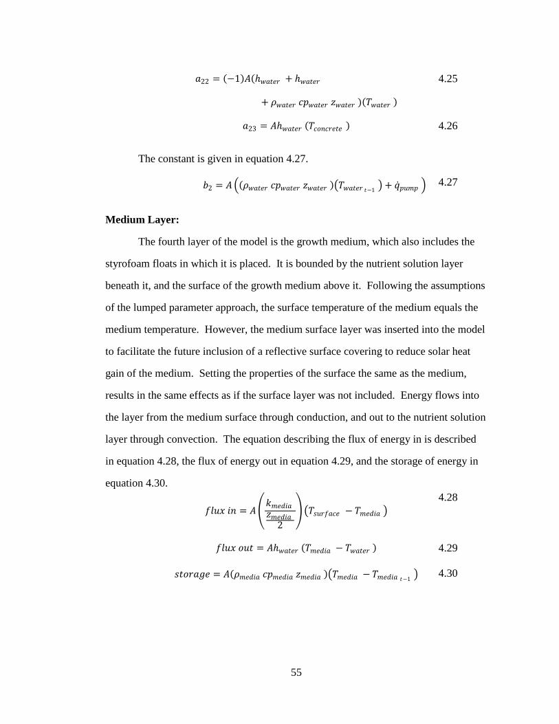
55
𝑎22 = −1 𝐴 𝑤𝑎𝑡𝑒𝑟 + 𝑤𝑎𝑡𝑒𝑟
+ 𝜌𝑤𝑎𝑡𝑒𝑟 𝑐𝑝𝑤𝑎𝑡𝑒𝑟 𝑧𝑤𝑎𝑡𝑒𝑟 𝑇𝑤𝑎𝑡𝑒𝑟
4.25
𝑎23 = 𝐴𝑤𝑎𝑡𝑒𝑟 𝑇𝑐𝑜𝑛𝑐𝑟𝑒𝑡𝑒 4.26
The constant is given in equation 4.27.
𝑏2 = 𝐴 𝜌𝑤𝑎𝑡𝑒𝑟 𝑐𝑝𝑤𝑎𝑡𝑒𝑟 𝑧𝑤𝑎𝑡𝑒𝑟 𝑇𝑤𝑎𝑡𝑒𝑟 𝑡−1 + 𝑞 𝑝𝑢𝑚𝑝 4.27
Medium Layer:
The fourth layer of the model is the growth medium, which also includes the
styrofoam floats in which it is placed. It is bounded by the nutrient solution layer
beneath it, and the surface of the growth medium above it. Following the assumptions
of the lumped parameter approach, the surface temperature of the medium equals the
medium temperature. However, the medium surface layer was inserted into the model
to facilitate the future inclusion of a reflective surface covering to reduce solar heat
gain of the medium. Setting the properties of the surface the same as the medium,
results in the same effects as if the surface layer was not included. Energy flows into
the layer from the medium surface through conduction, and out to the nutrient solution
layer through convection. The equation describing the flux of energy in is described
in equation 4.28, the flux of energy out in equation 4.29, and the storage of energy in
equation 4.30.
𝑓𝑙𝑢𝑥 𝑖𝑛 = 𝐴
𝑘𝑚𝑒𝑑𝑖𝑎𝑧𝑚𝑒𝑑𝑖𝑎
2
𝑇𝑠𝑢𝑟𝑓𝑎𝑐𝑒 − 𝑇𝑚𝑒𝑑𝑖𝑎
4.28
𝑓𝑙𝑢𝑥 𝑜𝑢𝑡 = 𝐴𝑤𝑎𝑡𝑒𝑟 𝑇𝑚𝑒𝑑𝑖𝑎 − 𝑇𝑤𝑎𝑡𝑒𝑟 4.29
𝑠𝑡𝑜𝑟𝑎𝑔𝑒 = 𝐴 𝜌𝑚𝑒𝑑𝑖𝑎 𝑐𝑝𝑚𝑒𝑑𝑖𝑎 𝑧𝑚𝑒𝑑𝑖𝑎 𝑇𝑚𝑒𝑑𝑖𝑎 − 𝑇𝑚𝑒𝑑𝑖𝑎 𝑡−1 4.30
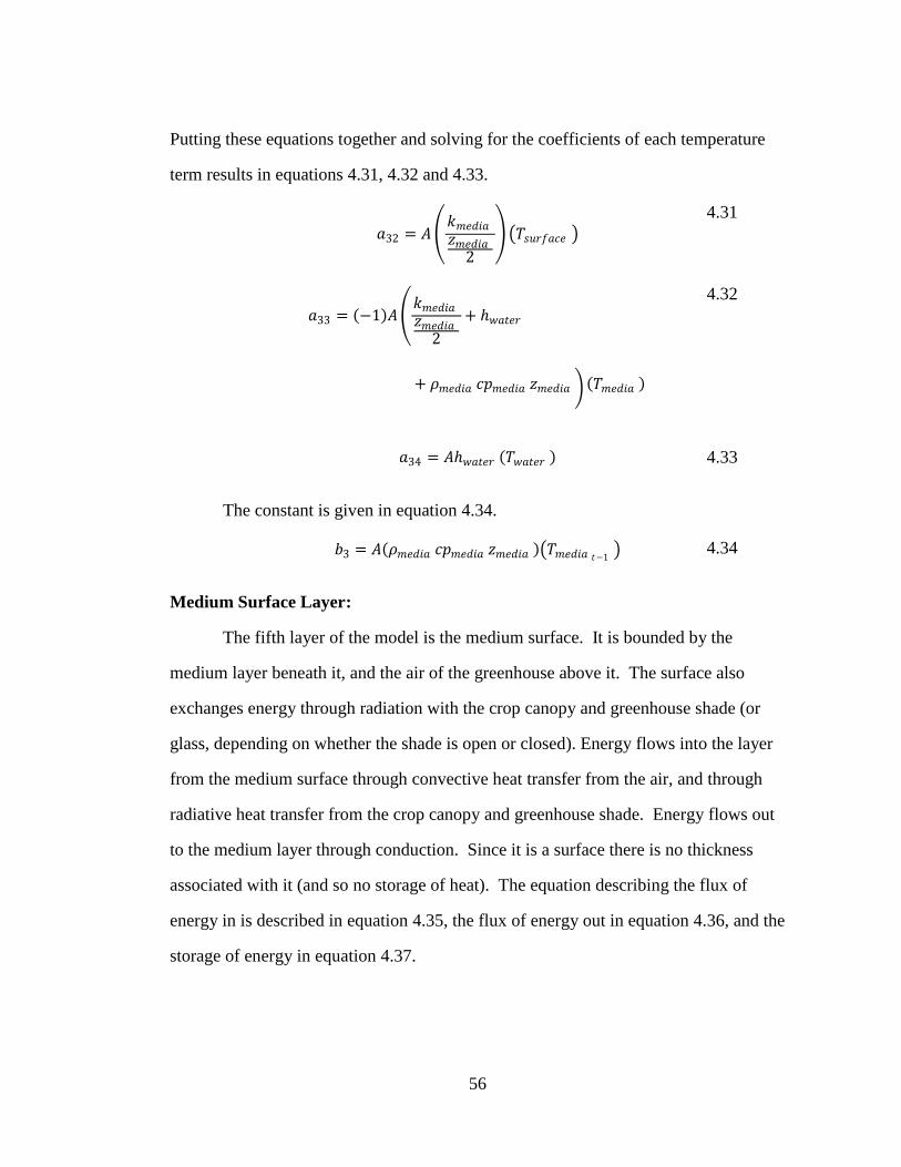
56
Putting these equations together and solving for the coefficients of each temperature
term results in equations 4.31, 4.32 and 4.33.
𝑎32 = 𝐴
𝑘𝑚𝑒𝑑𝑖𝑎𝑧𝑚𝑒𝑑𝑖𝑎
2
𝑇𝑠𝑢𝑟𝑓𝑎𝑐𝑒
4.31
𝑎33 = −1 𝐴
𝑘𝑚𝑒𝑑𝑖𝑎𝑧𝑚𝑒𝑑𝑖𝑎
2
+ 𝑤𝑎𝑡𝑒𝑟
+ 𝜌𝑚𝑒𝑑𝑖𝑎 𝑐𝑝𝑚𝑒𝑑𝑖𝑎 𝑧𝑚𝑒𝑑𝑖𝑎 𝑇𝑚𝑒𝑑𝑖𝑎
4.32
𝑎34 = 𝐴𝑤𝑎𝑡𝑒𝑟 𝑇𝑤𝑎𝑡𝑒𝑟 4.33
The constant is given in equation 4.34.
𝑏3 = 𝐴 𝜌𝑚𝑒𝑑𝑖𝑎 𝑐𝑝𝑚𝑒𝑑𝑖𝑎 𝑧𝑚𝑒𝑑𝑖𝑎 𝑇𝑚𝑒𝑑𝑖𝑎 𝑡−1
4.34
Medium Surface Layer:
The fifth layer of the model is the medium surface. It is bounded by the
medium layer beneath it, and the air of the greenhouse above it. The surface also
exchanges energy through radiation with the crop canopy and greenhouse shade (or
glass, depending on whether the shade is open or closed). Energy flows into the layer
from the medium surface through convective heat transfer from the air, and through
radiative heat transfer from the crop canopy and greenhouse shade. Energy flows out
to the medium layer through conduction. Since it is a surface there is no thickness
associated with it (and so no storage of heat). The equation describing the flux of
energy in is described in equation 4.35, the flux of energy out in equation 4.36, and the
storage of energy in equation 4.37.

57
𝑓𝑙𝑢𝑥 𝑖𝑛 = 𝐴 𝑚𝑒𝑑𝑖𝑎 −𝑎𝑖𝑟 𝑇𝑎𝑖𝑟1 − 𝑇𝑠𝑢𝑟𝑓𝑎𝑐𝑒
+ 1 − 𝜌𝑐𝑟𝑜𝑝 𝜃𝑠𝑜𝑙𝑎𝑟 ,𝑠𝑎𝑑𝑒 + 𝜃𝑙 𝑒−𝑘𝐿𝐴𝐼𝛼𝑚𝑒𝑑𝑖𝑎
+ 4𝐿𝐴𝐼휀𝑚𝑒𝑑𝑖𝑎 𝜍 𝑇𝑠𝑢𝑟𝑓𝑎𝑐𝑒 + 𝑇𝑐𝑟𝑜𝑝
2
3
𝑇𝑐𝑟𝑜𝑝
− 𝑇𝑠𝑢𝑟𝑓𝑎𝑐𝑒
+ 4 1
− 𝐿𝐴𝐼 휀𝑚𝑒𝑑𝑖𝑎 𝜍 𝑇𝑠𝑢𝑟𝑓𝑎𝑐𝑒 + 𝑇𝑠𝑎𝑑𝑒
2
3
𝑇𝑠𝑎𝑑𝑒
− 𝑇𝑠𝑢𝑟𝑓𝑎𝑐𝑒
4.35
𝑓𝑙𝑢𝑥 𝑜𝑢𝑡 = 𝐴
𝑘𝑚𝑒𝑑𝑖𝑎𝑧𝑚𝑒𝑑𝑖𝑎
2
𝑇𝑠𝑢𝑟𝑓𝑎𝑐𝑒 − 𝑇𝑚𝑒𝑑𝑖𝑎
4.36
𝑠𝑡𝑜𝑟𝑎𝑔𝑒 = 0 4.37
Putting these equations together and solving for the coefficients of each
temperature term results in equations 4.38, 4.39, 4.40, 4.41 and 4.42.
𝑎43 = 𝐴𝑚𝑒𝑑𝑖𝑎 −𝑎𝑖𝑟 𝑇𝑎𝑖𝑟1 4.38
𝑎44 = −1 𝐴 𝑚𝑒𝑑𝑖𝑎 −𝑎𝑖𝑟 + 4𝐿𝐴𝐼휀𝑚𝑒𝑑𝑖𝑎 𝜍
𝑇𝑠𝑢𝑟𝑓𝑎𝑐𝑒 + 𝑇𝑐𝑟𝑜𝑝
2
3
+ 4 1− 𝐿𝐴𝐼 휀𝑚𝑒𝑑𝑖𝑎 𝜍 𝑇𝑠𝑢𝑟𝑓𝑎𝑐𝑒 + 𝑇𝑠𝑎𝑑𝑒
2
3
+𝑘𝑚𝑒𝑑𝑖𝑎𝑧𝑚𝑒𝑑𝑖𝑎
2
𝑇𝑠𝑢𝑟𝑓𝑎𝑐𝑒
4.39

58
𝑎45 = 4𝐴𝐿𝐴𝐼휀𝑚𝑒𝑑𝑖𝑎 𝜍 𝑇𝑠𝑢𝑟𝑓𝑎𝑐𝑒 + 𝑇𝑐𝑟𝑜𝑝
2
3
𝑇𝑐𝑟𝑜𝑝 4.40
𝑎46 = 4𝐴 1− 𝐿𝐴𝐼 휀𝑚𝑒𝑑𝑖𝑎 𝜍 𝑇𝑠𝑢𝑟𝑓𝑎𝑐𝑒 + 𝑇𝑠𝑎𝑑𝑒
2
3
𝑇𝑠𝑎𝑑𝑒 4.41
𝑎47 = 𝐴
𝑘𝑚𝑒𝑑𝑖𝑎𝑧𝑚𝑒𝑑𝑖𝑎
2
𝑇𝑚𝑒𝑑𝑖𝑎
4.42
The constant is given in equation 4.43.
𝑏4 = −𝐴 1− 𝜌𝑐𝑟𝑜𝑝 𝜃𝑠𝑜𝑙𝑎𝑟 ,𝑠𝑎𝑑𝑒 + 𝜃𝑙 𝑒
−𝑘𝐿𝐴𝐼𝛼𝑚𝑒𝑑𝑖𝑎 4.43
Crop Canopy Layer:
The sixth layer of the model is the crop canopy. To simplify the interactions
with the crop canopy the assumption was made that the canopy is represented by the
Big Leaf model which assumes a single large leaf described by the Leaf Area Index,
rather than many smaller individual leaves. Energy flows into the layer from the
greenhouse air through convective heat transfer, through the absorption of sunlight
and supplemental lighting, and through radiative heat transfer from the greenhouse
shade. Some energy is gained by reflection of radiation from the medium surface,
however, this portion is assumed to be small and is omitted for simplicity. Energy
flows out through radiative exchange with the surface of the medium, and through
evapotranspiration. Since it is considered a surface there is no thickness associated
with it. The equation describing the flux of energy in is described in equation 4.44,
the flux of energy out in equation 4.45, and the storage of energy in equation 4.48.

59
𝑓𝑙𝑢𝑥 𝑖𝑛 = 𝐴 𝑐𝑟𝑜𝑝 −𝑎𝑖𝑟 𝑇𝑎𝑖𝑟1 − 𝑇𝑐𝑟𝑜𝑝
+ 1 − 𝜌𝑐𝑟𝑜𝑝 𝜃𝑠𝑜𝑙𝑎𝑟 ,𝑠𝑎𝑑𝑒 + 𝜃𝑙 1− 𝑒−𝑘𝐿𝐴𝐼 𝛼𝑐𝑟𝑜𝑝
+ 4𝐿𝐴𝐼휀𝑐𝑟𝑜𝑝 𝜍 𝑇𝑠𝑎𝑑𝑒 + 𝑇𝑐𝑟𝑜𝑝
2
3
𝑇𝑠𝑎𝑑𝑒 − 𝑇𝑐𝑟𝑜𝑝
4.44
𝑓𝑙𝑢𝑥 𝑜𝑢𝑡 = 𝐴 4𝐿𝐴𝐼휀𝑚𝑒𝑑𝑖𝑎 𝜍
𝑇𝑠𝑢𝑟𝑓𝑎𝑐𝑒 + 𝑇𝑐𝑟𝑜𝑝
2
3
𝑇𝑐𝑟𝑜𝑝 − 𝑇𝑠𝑢𝑟𝑓𝑎𝑐𝑒
+ 𝐸𝑇
4.45
Evapotranspiration (ET) is determined by using the Penman-Monteith method (Pereira
et al., 1996) to calculate the reference evapotranspiration. For simplification it was
assumed that soil heat flux (G) was equal to zero.
𝐸𝑇𝑜 =
𝐻𝑓𝑔𝜌𝑤𝑎𝑡𝑒𝑟 𝐾𝑐
0.408∆ 𝑅𝑛 − 𝐺 + 𝛾 900
𝑇𝑎𝑖𝑟 ,𝑡−1 + 273.15 𝑈2 𝑒𝑎 − 𝑒𝑑
∆+ 𝛾 1 + 0.34𝑈2
4.46
To convert the reference crop evapotranspiration to an evapotranspiration similar to
spinach, it is necessary to multiply by a crop coefficient, Kc. It was assumed that
spinach transpires in a similar fashion to lettuce, for which Ciolkosz and Albright
(2000) determined a value of 1.84 for Kc. It is also necessary to convert the depth of
water into an energy equivalent which is done by multiplying by the heat of
vaporization of water at the canopy temperature (Hfg).
𝐸𝑇 = 𝐻𝑓𝑔𝜌𝑤𝑎𝑡𝑒𝑟 𝐾𝑐𝐸𝑇𝑜 4.47
𝑠𝑡𝑜𝑟𝑎𝑔𝑒 = 0 4.48
60
Putting these equations together and solving for the coefficients of each
temperature term results in equations 4.49, 4.50, 4.51, and 4.52.
𝑎54 = 𝐴𝑐𝑟𝑜𝑝 −𝑎𝑖𝑟 𝑇𝑎𝑖𝑟1 4.49
𝑎55
= −1 𝐴 𝑐𝑟𝑜𝑝 −𝑎𝑖𝑟
+ 4𝐿𝐴𝐼휀𝑐𝑟𝑜𝑝 𝜍 𝑇𝑠𝑎𝑑𝑒 + 𝑇𝑐𝑟𝑜𝑝
2
3
4𝐿𝐴𝐼휀𝑚𝑒𝑑𝑖𝑎 𝜍 𝑇𝑠𝑢𝑟𝑓𝑎𝑐𝑒 + 𝑇𝑐𝑟𝑜𝑝
2
3
𝑇𝑐𝑟𝑜𝑝
4.50
𝑎56 = 4𝐴𝐿𝐴𝐼휀𝑐𝑟𝑜𝑝 𝜍 𝑇𝑠𝑎𝑑𝑒 + 𝑇𝑐𝑟𝑜𝑝
2
3
𝑇𝑠𝑎𝑑𝑒
4.51
𝑎57 = 4𝐴𝐿𝐴𝐼휀𝑚𝑒𝑑𝑖𝑎 𝜍 𝑇𝑠𝑢𝑟𝑓𝑎𝑐𝑒 + 𝑇𝑐𝑟𝑜𝑝
2
3
𝑇𝑠𝑢𝑟𝑓𝑎𝑐𝑒 4.52
The constant is given in equation 4.53.
𝑏5 = −1 𝐴 1− 𝜌𝑐𝑟𝑜𝑝 𝜃𝑠𝑜𝑙𝑎𝑟 ,𝑠𝑎𝑑𝑒 + 𝜃𝑙 1− 𝑒−𝑘𝐿𝐴𝐼 𝛼𝑐𝑟𝑜𝑝
+ 𝐸𝑇
4.53
Greenhouse Air Layer (below the shade):
The seventh layer of the model is the air in the greenhouse below the shade
canopy. Energy flows into the layer from the bulk flow of air from above the shade,
outside the greenhouse through infiltration, and through the air vents, which,
depending on whether the cooling pads are operating, may be either outdoor air, or
cooled air. This greenhouse air layer also receives energy from convective heat
transfer from the shade curtain, as well as from the greenhouse heater (if functioning),
and from the supplemental lights, if they are on. Evapotranspiration is also considered

61
an energy input to this layer. Energy flows out through convective heat transfer with
the crop canopy and the medium surface, as well as through the exchange of air from
above the shade curtain, and to the outside through infiltration and venting.
The equation describing the flux of energy in is described in equation 4.54, the
flux of energy out in equation 4.55, and the storage of energy in equation 4.56.
𝑓𝑙𝑢𝑥 𝑖𝑛
= 𝐴 𝑞 𝑒𝑎𝑡𝑒𝑟 + 𝑞 𝑙𝑎𝑚𝑝𝑠
+ 𝐸𝑇 + 𝑠𝑎𝑑𝑒 −𝑎𝑖𝑟1 𝑇𝑠𝑎𝑑𝑒 − 𝑇𝑎𝑖𝑟1
+ 𝑣1
𝑉𝑠𝑎 𝑣𝑒𝑛𝑡 1006 𝑇𝑣𝑒𝑛𝑡 − 273.15
+𝑊𝑣𝑒𝑛𝑡 2501000
+ 1805 𝑇𝑣𝑒𝑛𝑡 − 273.15
+ 𝑛𝑉1−𝑉2
𝑉𝑠𝑎 𝑎𝑖𝑟2
1006 𝑇𝑎𝑖𝑟2 − 273.15
+𝑊𝑎𝑖𝑟2 2501000
+ 1805 𝑇𝑎𝑖𝑟2 − 273.15
+ 𝑛1
𝑉𝑠𝑎 𝑎𝑚𝑏 1006 𝑇𝑎𝑚𝑏 − 273.15
+𝑊𝑎𝑚𝑏 2501000
+ 1805 𝑇𝑎𝑚𝑏 − 273.15
4.54

62
𝑓𝑙𝑢𝑥 𝑜𝑢𝑡 = 𝐴 𝑐𝑟𝑜𝑝 −𝑎𝑖𝑟 𝑇𝑎𝑖𝑟1 − 𝑇𝑐𝑟𝑜𝑝
+ 𝑚𝑒𝑑𝑖𝑎 −𝑎𝑖𝑟 𝑇𝑎𝑖𝑟1 − 𝑇𝑠𝑢𝑟𝑓𝑎𝑐𝑒
+ 𝑣1
𝑉𝑠𝑎 𝑎𝑖𝑟1
1006 𝑇𝑎𝑖𝑟1 − 273.15
+𝑊𝑎𝑖𝑟1 2501000 + 1805 𝑇𝑎𝑖𝑟1 − 273.15
+ 𝑛𝑉1−𝑉2
𝑉𝑠𝑎 𝑎𝑖𝑟1
1006 𝑇𝑎𝑖𝑟1 − 273.15
+𝑊𝑎𝑖𝑟1 2501000 + 1805 𝑇𝑎𝑖𝑟1 − 273.15
+ 𝑛1
𝑉𝑠𝑎 𝑎𝑖𝑟1
1006 𝑇𝑎𝑖𝑟1 − 273.15
+𝑊𝑎𝑖𝑟1 2501000 + 1805 𝑇𝑎𝑖𝑟1 − 273.15
4.55
𝑠𝑡𝑜𝑟𝑎𝑔𝑒 =
𝑉1
𝑉𝑠𝑎 𝑎𝑖𝑟1
1006 𝑇𝑎𝑖𝑟1 − 273.15
+𝑊𝑎𝑖𝑟1 2501000 + 1805 −273.15
− 𝑉1
𝑉𝑠𝑎 𝑎𝑖𝑟1𝑡−1
1006 𝑇𝑎𝑖𝑟1𝑡−1− 273.15
+𝑊𝑎𝑖𝑟1𝑡−1 2501000
+ 1805 𝑇𝑎𝑖𝑟1𝑡−1− 273.15
4.56
63
Putting these equations together and solving for the coefficients of each
temperature term results in equations 4.57, 4.58, 4.59, 4.60 and 4.61.
𝑎64 = 𝐴𝑚𝑒𝑑𝑖𝑎 −𝑎𝑖𝑟 𝑇𝑠𝑢𝑟𝑓𝑎𝑐𝑒
4.57
𝑎65 = 𝐴𝑐𝑟𝑜𝑝 −𝑎𝑖𝑟 𝑇𝑐𝑟𝑜𝑝 4.58
𝑎66
= −1 𝐴 𝑠𝑎𝑑𝑒 −𝑎𝑖𝑟1 + 𝑐𝑟𝑜𝑝 −𝑎𝑖𝑟 + 𝑚𝑒𝑑𝑖𝑎 −𝑎𝑖𝑟
+ 1006 +𝑊𝑎𝑖𝑟1 ∗ 1805 𝑛1 + 𝑉1 + 𝑣1 + 𝑛𝑉1−𝑉2
𝑉𝑠𝑎1𝑡−1
𝑇𝑎𝑖𝑟1
4.59
𝑎67 = 𝐴𝑠𝑎𝑑𝑒 −𝑎𝑖𝑟1 𝑇𝑠𝑎𝑑𝑒 4.60
𝑎68 = 1006 +𝑊𝑎𝑖𝑟2 ∗ 1805 𝑛𝑉1−𝑉2
𝑉𝑠𝑎2𝑡−1
𝑇𝑎𝑖𝑟2 4.61
The constant is given in equation 4.62.

64
𝑏6 = −1 𝐴 𝑞 𝑒𝑎𝑡𝑒𝑟 + 𝑞 𝑙𝑎𝑚𝑝𝑠 + 𝐸𝑇
+ 𝑣1
𝑉𝑠𝑎 𝑣𝑒𝑛𝑡 1006 𝑇𝑣𝑒𝑛𝑡 − 273.15
+𝑊𝑣𝑒𝑛𝑡 2501000 + 1805 𝑇𝑣𝑒𝑛𝑡 − 273.15
+ 𝑛1
𝑉𝑠𝑎 𝑎𝑚𝑏 1006 𝑇𝑎𝑚𝑏 − 273.15
+𝑊𝑎𝑚𝑏 2501000 + 1805 𝑇𝑎𝑚𝑏 − 273.15
− 𝑛1 + 𝑉1 + 𝑣1 + 𝑛𝑉1−𝑉2
𝑉𝑠𝑎 𝑎𝑖𝑟1𝑡−1
1006 −273.15
+𝑊𝑎𝑖𝑟1 2501000 + 1805 −273.15
+ 𝑛𝑉1−𝑉2
𝑉𝑠𝑎 𝑎𝑖𝑟2𝑡−1
1006 −273.15
+𝑊𝑎𝑖𝑟2 2501000 + 1805 −273.15
+ 𝑉1
𝑉𝑠𝑎 𝑎𝑖𝑟1𝑡−1
1006 𝑇𝑎𝑖𝑟1𝑡−1− 273.15
+𝑊𝑎𝑖𝑟1𝑡−1 2501000 + 1805 𝑇𝑎𝑖𝑟1𝑡−1
− 273.15
4.62
Shade Layer:
The eighth layer of the model is the shade canopy. For the purposes of the
model it is assumed to have no thickness (no heat storage). Energy flows into the
shade through convection exchange with the greenhouse air layer above the shade
(and below the glass), through radiative exchange with the greenhouse glass, and from
the portion of sunlight passing through the glass that the shade intercepts. Energy
flows out from the shade through convective exchange with the air layer beneath the

65
shade, and through radiative exchange with both the crop canopy and medium surface.
The equation describing the flux of energy in is described in equation 4.63, the flux of
energy out in equation 4.64, and the storage of energy in equation 4.65.
𝑓𝑙𝑢𝑥 𝑖𝑛 = 𝐴 𝑠𝑎𝑑𝑒−𝑎𝑖𝑟2 𝑇𝑎𝑖𝑟2 − 𝑇𝑠𝑎𝑑𝑒
+ 4휀𝑔𝑙𝑎𝑠𝑠 𝜍 𝑇𝑔𝑙𝑎𝑠𝑠 + 𝑇𝑠𝑎𝑑𝑒
2
3
𝑇𝑔𝑙𝑎𝑠𝑠−𝑇𝑠𝑎𝑑𝑒
+ 1− 𝜌𝑔𝑙𝑎𝑠𝑠 𝜃𝑠𝑜𝑙𝑎𝑟 ,𝑔𝑙𝑎𝑠𝑠 𝛼𝑠𝑎𝑑𝑒
4.63
𝑓𝑙𝑢𝑥 𝑜𝑢𝑡 = 𝐴 𝑠𝑎𝑑𝑒 −𝑎𝑖𝑟1 𝑇𝑠𝑎𝑑𝑒 − 𝑇𝑎𝑖𝑟1
+ 4 1
− 𝐿𝐴𝐼 휀𝑚𝑒𝑑𝑖𝑎 𝜍 𝑇𝑠𝑢𝑟𝑓𝑎𝑐𝑒 + 𝑇𝑠𝑎𝑑𝑒
2
3
𝑇𝑠𝑎𝑑𝑒
− 𝑇𝑠𝑢𝑟𝑓𝑎𝑐𝑒
+ 4 𝐿𝐴𝐼 휀𝑐𝑟𝑜𝑝 𝜍 𝑇𝑠𝑎𝑑𝑒 + 𝑇𝑐𝑟𝑜𝑝
2
3
𝑇𝑠𝑎𝑑𝑒
− 𝑇𝑐𝑟𝑜𝑝
4.64
𝑠𝑡𝑜𝑟𝑎𝑔𝑒 = 0 4.65
Putting these equations together and solving for the coefficients of each
temperature term results in equations 4.66, 4.67, 4.68, 4.69, 4.70 and 4.71.
𝑎74 = 4𝐴 1 − 𝐿𝐴𝐼 휀𝑚𝑒𝑑𝑖𝑎 𝜍
𝑇𝑠𝑢𝑟𝑓𝑎𝑐𝑒 + 𝑇𝑠𝑎𝑑𝑒
2
3
𝑇𝑠𝑢𝑟𝑓𝑎𝑐𝑒 4.66
𝑎75 = 4𝐴 𝐿𝐴𝐼 휀𝑐𝑟𝑜𝑝 𝜍 𝑇𝑠𝑎𝑑𝑒 + 𝑇𝑐𝑟𝑜𝑝
2
3
𝑇𝑐𝑟𝑜𝑝 4.67

66
𝑎76 = 𝐴𝑠𝑎𝑑𝑒 −𝑎𝑖𝑟1 𝑇𝑎𝑖𝑟1
4.68
𝑎77 = −1 𝐴 𝑠𝑎𝑑𝑒 −𝑎𝑖𝑟2 + 4휀𝑔𝑙𝑎𝑠𝑠 𝜍 𝑇𝑔𝑙𝑎𝑠𝑠 + 𝑇𝑠𝑎𝑑𝑒
2
3
+ 𝑠𝑎𝑑𝑒 −𝑎𝑖𝑟1
+ 4 1− 𝐿𝐴𝐼 휀𝑚𝑒𝑑𝑖𝑎 𝜍 𝑇𝑠𝑢𝑟𝑓𝑎𝑐𝑒 + 𝑇𝑠𝑎𝑑𝑒
2
3
+ 4 𝐿𝐴𝐼 휀𝑐𝑟𝑜𝑝 𝜍 𝑇𝑠𝑎𝑑𝑒 + 𝑇𝑐𝑟𝑜𝑝
2
3
𝑇𝑠𝑎𝑑𝑒
4.69
𝑎78 = 𝐴𝑠𝑎𝑑𝑒 −𝑎𝑖𝑟2 𝑇𝑎𝑖𝑟2
4.70
𝑎79 = 4𝐴휀𝑔𝑙𝑎𝑠𝑠 𝜍 𝑇𝑔𝑙𝑎𝑠𝑠 + 𝑇𝑠𝑎𝑑𝑒
2
3
𝑇𝑔𝑙𝑎𝑠𝑠
4.71
The constant is given in equation 4.72.
𝑏7 = (−1)𝐴 1− 𝜌𝑔𝑙𝑎𝑠𝑠 𝜃𝑠𝑜𝑙𝑎𝑟 ,𝑔𝑙𝑎𝑠𝑠 𝛼𝑠𝑎𝑑𝑒 4.72
Greenhouse Air Layer (above shade):
The ninth layer of the model is the air above the shade curtain. Energy flows
into the layer through convective exchange with the greenhouse glass. Energy also
flows into this air layer through the bulk exchange of air with the outside through
infiltration, and with the layer below the shade. Energy flows out of the layer through
convective exchange with the shade curtain and through the exchange of air with
outside air and the air layer below the shade through infiltration. The equation

67
describing the flux of energy in is described in equation 4.73, the flux of energy out in
equation 4.74, and the storage of energy in equation 4.75.
𝑓𝑙𝑢𝑥 𝑖𝑛 = 𝐴𝑔𝑙𝑎𝑠𝑠 −𝑎𝑖𝑟2 𝑇𝑔𝑙𝑎𝑠𝑠 − 𝑇𝑎𝑖𝑟2
+ 𝑛2
𝑉𝑠𝑎 𝑎𝑚𝑏 1006 𝑇𝑎𝑚𝑏 − 273.15
+𝑊𝑎𝑚𝑏 2501000 + 1805 𝑇𝑎𝑚𝑏 − 273.15
+ 𝑛𝑉1−𝑉2
𝑉𝑠𝑎 𝑎𝑖𝑟1
1006 𝑇𝑎𝑖𝑟1 − 273.15
+𝑊𝑎𝑖𝑟1 2501000 + 1805 𝑇𝑎𝑖𝑟1 − 273.15
4.73
𝑓𝑙𝑢𝑥 𝑜𝑢𝑡
= 𝐴𝑠𝑎𝑑𝑒 −𝑎𝑖𝑟2 𝑇𝑎𝑖𝑟2 − 𝑇𝑠𝑎𝑑𝑒
+ 𝑛2
𝑉𝑠𝑎 𝑎𝑖𝑟2
1006 𝑇𝑎𝑖𝑟2 − 273.15
+𝑊𝑎𝑖𝑟2 2501000
+ 1805 𝑇𝑎𝑖𝑟2 − 273.15
+ 𝑛𝑉1−𝑉2
𝑉𝑠𝑎 𝑎𝑖𝑟2
1006 𝑇𝑎𝑖𝑟2 − 273.15
+𝑊𝑎𝑖𝑟2 2501000
+ 1805 𝑇𝑎𝑖𝑟2 − 273.15
4.74
68
𝑠𝑡𝑜𝑟𝑎𝑔𝑒 =
𝑉2
𝑉𝑠𝑎 𝑎𝑖𝑟2
1006 𝑇𝑎𝑖𝑟2 − 273.15
+𝑊𝑎𝑖𝑟2 2501000 + 1805 −273.15
− 𝑉2
𝑉𝑠𝑎 𝑎𝑖𝑟2𝑡−1
1006 𝑇𝑎𝑖𝑟2𝑡−1− 273.15
+𝑊𝑎𝑖𝑟2𝑡−1 2501000
+ 1805 𝑇𝑎𝑖𝑟2𝑡−1− 273.15
4.75
Putting these equations together and solving for the coefficients of each
temperature term results in equations 4.76, 4.77, 4.78, and 4.79.
𝑎86 = 1006 +𝑊𝑎𝑖𝑟1 ∗ 1805 𝑛𝑉1−𝑉2
𝑉𝑠𝑎1𝑡−1
𝑇𝑎𝑖𝑟1
4.76
𝑎87 = 𝐴𝑠𝑎𝑑𝑒 −𝑎𝑖𝑟2 𝑇𝑠𝑎𝑑𝑒
4.77
𝑎88
= −1 𝐴 𝑔𝑙𝑎𝑠𝑠 −𝑎𝑖𝑟2 + 𝑠𝑎𝑑𝑒 −𝑎𝑖𝑟2
+ 1006 +𝑊𝑎𝑖𝑟2 ∗ 1805 𝑛2 + 𝑉2 + 𝑛𝑉1−𝑉2
𝑉𝑠𝑎2𝑡−1
𝑇𝑎𝑖𝑟2
4.78
𝑎89 = 𝐴𝑔𝑙𝑎𝑠𝑠 −𝑎𝑖𝑟2 𝑇𝑔𝑙𝑎𝑠𝑠
4.79

69
The constant is given in equation 4.80.
𝑏8 = −1 𝑛2
𝑉𝑠𝑎 𝑎𝑚𝑏 1006 𝑇𝑎𝑚𝑏 − 273.15
+𝑊𝑎𝑚𝑏 2501000 + 1805 𝑇𝑎𝑚𝑏 − 273.15
+ 𝑉2
𝑉𝑠𝑎 𝑎𝑖𝑟2𝑡−1
1006 𝑇𝑎𝑖𝑟2𝑡−1− 273.15
+𝑊𝑎𝑖𝑟2𝑡−1 2501000
+ 1805 𝑇𝑎𝑖𝑟2𝑡−1− 273.15
+ 𝑛𝑉1−𝑉2
𝑉𝑠𝑎 𝑎𝑖𝑟1𝑡−1
1006 −273.15
+𝑊𝑎𝑖𝑟1 2501000 + 1805 −273.15
− 𝑛2 + 𝑉2 + 𝑛𝑉1−𝑉2
𝑉𝑠𝑎 𝑎𝑖𝑟2𝑡−1
1006 −273.15
+𝑊𝑎𝑖𝑟2 2501000 + 1805 −273.15
4.80
Greenhouse Glass Layer:
The tenth and final layer of the model is the greenhouse glass. For the
purposes of the model it is assumed to have no thickness, store no heat and have
negligible thermal resistance. Energy flow into the glass is from convective exchange
with the outside (ambient) air, from the portion of the sunlight the glass intercepts, and
from radiative exchange with the sky. As the temperature of the sky is not provided in

70
the data file which this simulation uses, an estimate for the temperature of the sky was
used, based on the relation (Swinbank 1963):
𝑇𝑠𝑘𝑦 = 0.0552𝑇𝑎𝑚𝑏
1.5 4.81
This relation is valid for a clear sky and does not really work for a cloudy sky situation
which is significantly more complex. However, the clear sky approach was used as a
quick approximation sufficient for the purpose of the overall greenhouse simulation
model.
Energy flows out from the layer through convection exchange with the air
layer below, and through radiative exchange with the shade curtain. The equation
describing the flux of energy in, is described in equation 4.82, the flux of energy out in
equation 4.83, and the storage of energy in equation 4.84.
𝑓𝑙𝑢𝑥 𝑖𝑛 = 𝐴 𝑔𝑙𝑎𝑠𝑠 −𝑎𝑚𝑏𝑖𝑒𝑛𝑡 𝑇𝑎𝑚𝑏𝑖𝑒𝑛𝑡 − 𝑇𝑔𝑙𝑎𝑠𝑠
+ 1− 𝜌𝑔𝑙𝑎𝑠𝑠 𝜃𝑠𝑜𝑙𝑎𝑟 ,𝑜𝑢𝑡𝑠𝑖𝑑𝑒 𝛼𝑔𝑙𝑎𝑠𝑠
+ 4휀𝑔𝑙𝑎𝑠𝑠 𝜍 𝑇𝑔𝑙𝑎𝑠𝑠 + 𝑇𝑠𝑘𝑦
2
3
𝑇𝑠𝑘𝑦 − 𝑇𝑔𝑙𝑎𝑠𝑠
4.82
𝑓𝑙𝑢𝑥 𝑜𝑢𝑡 = 𝐴 𝑔𝑙𝑎𝑠𝑠 −𝑎𝑖𝑟2 𝑇𝑔𝑙𝑎𝑠𝑠 − 𝑇𝑎𝑖𝑟2
+ 4휀𝑔𝑙𝑎𝑠𝑠 𝜍 𝑇𝑔𝑙𝑎𝑠𝑠 + 𝑇𝑠𝑎𝑑𝑒
2
3
𝑇𝑔𝑙𝑎𝑠𝑠
− 𝑇𝑠𝑎𝑑𝑒
4.83

71
𝑠𝑡𝑜𝑟𝑎𝑔𝑒 = 0 4.84
Putting these equations together and solving for the coefficients of each
temperature term results in equations 4.85, 4.86, and 4.87.
𝑎97 = 4𝐴휀𝑔𝑙𝑎𝑠𝑠 𝜍 𝑇𝑔𝑙𝑎𝑠𝑠 + 𝑇𝑠𝑎𝑑𝑒
2
3
𝑇𝑠𝑎𝑑𝑒 4.85
𝑎98 = −1 𝐴 𝑔𝑙𝑎𝑠𝑠 −𝑎𝑚𝑏𝑖𝑒𝑛𝑡 + 4휀𝑔𝑙𝑎𝑠𝑠 𝜍 𝑇𝑔𝑙𝑎𝑠𝑠 + 𝑇𝑠𝑘𝑦
2
3
+ 𝑔𝑙𝑎𝑠𝑠 −𝑎𝑖𝑟2
+ 4휀𝑔𝑙𝑎𝑠𝑠 𝜍 𝑇𝑔𝑙𝑎𝑠𝑠 + 𝑇𝑠𝑎𝑑𝑒
2
3
𝑇𝑔𝑙𝑎𝑠𝑠
4.86
𝑎99 = 𝐴𝑔𝑙𝑎𝑠𝑠 −𝑎𝑖𝑟2 𝑇𝑎𝑖𝑟2
4.87
The constant is given in equation 4.88.
𝑏9 = −1 𝐴 𝑔𝑙𝑎𝑠𝑠 −𝑎𝑚𝑏𝑖𝑒𝑛𝑡 𝑇𝑎𝑚𝑏𝑖𝑒𝑛𝑡
+ 1− 𝜌𝑔 𝜃𝑠𝑜𝑙𝑎𝑟 ,𝑜𝑢𝑡𝑠𝑖𝑑𝑒 𝛼𝑔𝑙𝑎𝑠𝑠
+ 4휀𝑔𝑙𝑎𝑠𝑠 𝜍 𝑇𝑔𝑙𝑎𝑠𝑠 + 𝑇𝑠𝑘𝑦
2
3
𝑇𝑠𝑘𝑦
4.88

72
Greenhouse Model Without Shade Curtain
The model implements light and shade control, and decisions about the status
of the lights and shade are made every hour. Depending on whether the shade is
opened or closed the number of layers of the model changes. If the shade is open, the
shade layer drops out, and the two greenhouse airspaces are combined. If this is the
case the model temperatures can be solved by putting the calculated coefficients into
an 8 x 8 matrix (equation 4.89), inverting it, and then multiplying by the solution
matrix (b0, b1, …, b7) to get the temperatures of the 8 layers.
a00 a01 0 0 0 0 0 0
Tsoil
b0 a10 a11 a12 0 0 0 0 0
Tconcrete
b1 0 a21 a22 a23 0 0 0 0
Twater
b2 0 0 a32 a33 a34 0 0 0 x Tmedium = b3 0 0 0 a43 a44 a45 a46 a47
Tsurface
b4 0 0 0 0 a54 a55 a56 a57
Tcanopy
b5 0 0 0 0 a64 a65 a66 a67
Tair
b6
0 0 0 0 a74 a75 a76 a77
Tglass
b7
4.89
The equations governing the soil to medium layers remain unchanged;
however, the remaining layers have new equations as follow.
Medium Surface Layer:
The equation for the medium surface is nearly identical. The only difference is
that rather than radiative exchange with the shade curtain, the radiative exchange is
now directly with the greenhouse glass. All other energy exchanges remain the same.
The equation describing the flux of energy in is described in equation 4.90, the flux of
energy out in equation 4.91, and the storage of energy in equation 4.92.
73
𝑓𝑙𝑢𝑥 𝑖𝑛 = 𝐴 𝑚𝑒𝑑𝑖𝑎 −𝑎𝑖𝑟 𝑇𝑎𝑖𝑟 − 𝑇𝑠𝑢𝑟𝑓𝑎𝑐𝑒
+ 1 − 𝜌𝑐𝑟𝑜𝑝 𝜃𝑠𝑜𝑙𝑎𝑟 ,𝑠𝑎𝑑𝑒 + 𝜃𝑙 𝑒−𝑘𝐿𝐴𝐼𝛼𝑚𝑒𝑑𝑖𝑎
+ 4𝐿𝐴𝐼휀𝑚𝑒𝑑𝑖𝑎 𝜍 𝑇𝑠𝑢𝑟𝑓𝑎𝑐𝑒 + 𝑇𝑐𝑟𝑜𝑝
2
3
𝑇𝑐𝑟𝑜𝑝
− 𝑇𝑠𝑢𝑟𝑓𝑎𝑐𝑒
+ 4 1
− 𝐿𝐴𝐼 휀𝑚𝑒𝑑𝑖𝑎 𝜍 𝑇𝑠𝑢𝑟𝑓𝑎𝑐𝑒 + 𝑇𝑔𝑙𝑎𝑠𝑠
2
3
𝑇𝑔𝑙𝑎𝑠𝑠
− 𝑇𝑠𝑢𝑟𝑓𝑎𝑐𝑒
4.90
𝑓𝑙𝑢𝑥 𝑜𝑢𝑡 = 𝐴
𝑘𝑚𝑒𝑑𝑖𝑎𝑧𝑚𝑒𝑑𝑖𝑎
2
𝑇𝑠𝑢𝑟𝑓𝑎𝑐𝑒 − 𝑇𝑚𝑒𝑑𝑖𝑎
4.91
𝑠𝑡𝑜𝑟𝑎𝑔𝑒 = 0 4.92
Putting these equations together and solving for the coefficients of each
temperature term results in equations 4.93, 4.94, 4.95, 4.96 and 4.97.
𝑎43 = 𝐴𝑚𝑒𝑑𝑖𝑎 −𝑎𝑖𝑟 𝑇𝑎𝑖𝑟 4.93
𝑎44 = −1 𝐴 𝑚𝑒𝑑𝑖𝑎 −𝑎𝑖𝑟 + 4𝐿𝐴𝐼휀𝑚𝑒𝑑𝑖𝑎 𝜍 𝑇𝑠𝑢𝑟𝑓𝑎𝑐𝑒 + 𝑇𝑐𝑟𝑜𝑝
2
3
+ 4 1− 𝐿𝐴𝐼 휀𝑚𝑒𝑑𝑖𝑎 𝜍 𝑇𝑠𝑢𝑟𝑓𝑎𝑐𝑒 + 𝑇𝑔𝑙𝑎𝑠𝑠
2
3
+𝑘𝑚𝑒𝑑𝑖𝑎𝑧𝑚𝑒𝑑𝑖𝑎
2
𝑇𝑠𝑢𝑟𝑓𝑎𝑐𝑒
4.94
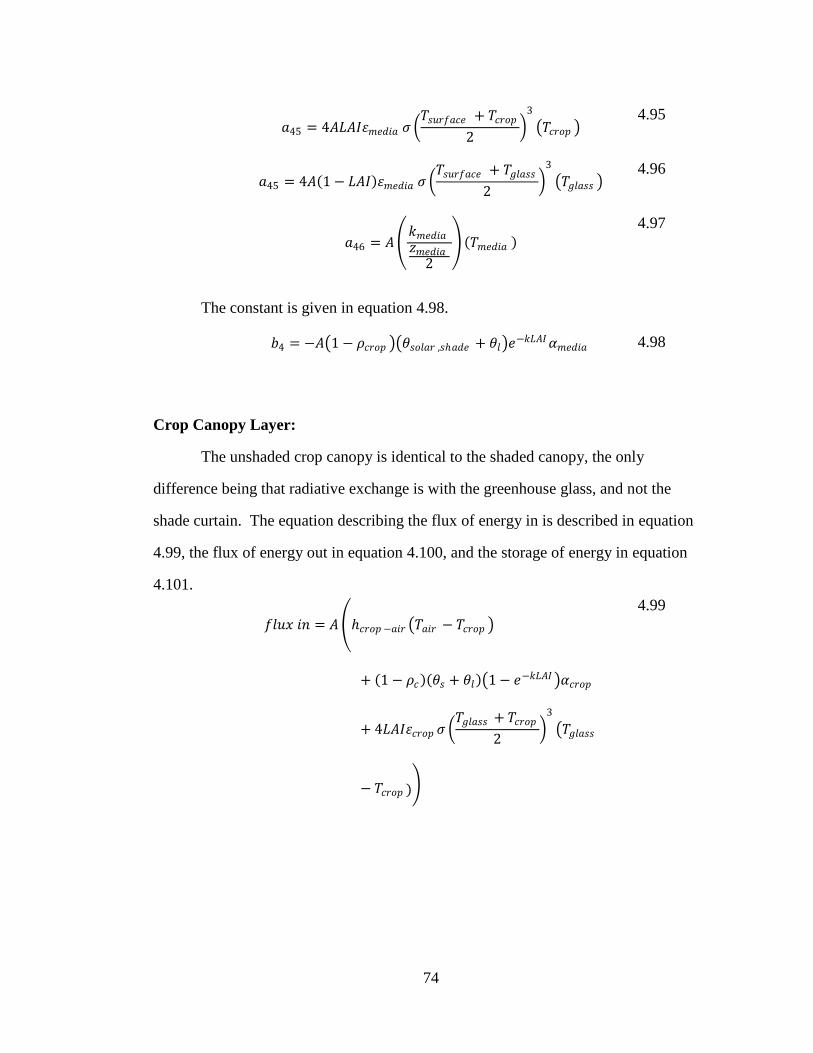
74
𝑎45 = 4𝐴𝐿𝐴𝐼휀𝑚𝑒𝑑𝑖𝑎 𝜍 𝑇𝑠𝑢𝑟𝑓𝑎𝑐𝑒 + 𝑇𝑐𝑟𝑜𝑝
2
3
𝑇𝑐𝑟𝑜𝑝 4.95
𝑎45 = 4𝐴 1− 𝐿𝐴𝐼 휀𝑚𝑒𝑑𝑖𝑎 𝜍
𝑇𝑠𝑢𝑟𝑓𝑎𝑐𝑒 + 𝑇𝑔𝑙𝑎𝑠𝑠
2
3
𝑇𝑔𝑙𝑎𝑠𝑠 4.96
𝑎46 = 𝐴
𝑘𝑚𝑒𝑑𝑖𝑎𝑧𝑚𝑒𝑑𝑖𝑎
2
𝑇𝑚𝑒𝑑𝑖𝑎
4.97
The constant is given in equation 4.98.
𝑏4 = −𝐴 1− 𝜌𝑐𝑟𝑜𝑝 𝜃𝑠𝑜𝑙𝑎𝑟 ,𝑠𝑎𝑑𝑒 + 𝜃𝑙 𝑒
−𝑘𝐿𝐴𝐼𝛼𝑚𝑒𝑑𝑖𝑎 4.98
Crop Canopy Layer:
The unshaded crop canopy is identical to the shaded canopy, the only
difference being that radiative exchange is with the greenhouse glass, and not the
shade curtain. The equation describing the flux of energy in is described in equation
4.99, the flux of energy out in equation 4.100, and the storage of energy in equation
4.101.
𝑓𝑙𝑢𝑥 𝑖𝑛 = 𝐴 𝑐𝑟𝑜𝑝 −𝑎𝑖𝑟 𝑇𝑎𝑖𝑟 − 𝑇𝑐𝑟𝑜𝑝
+ 1− 𝜌𝑐 𝜃𝑠 + 𝜃𝑙 1− 𝑒−𝑘𝐿𝐴𝐼 𝛼𝑐𝑟𝑜𝑝
+ 4𝐿𝐴𝐼휀𝑐𝑟𝑜𝑝 𝜍 𝑇𝑔𝑙𝑎𝑠𝑠 + 𝑇𝑐𝑟𝑜𝑝
2
3
𝑇𝑔𝑙𝑎𝑠𝑠
− 𝑇𝑐𝑟𝑜𝑝
4.99

75
𝑓𝑙𝑢𝑥 𝑜𝑢𝑡 = 𝐴 4𝐿𝐴𝐼휀𝑚𝑒𝑑𝑖𝑎 𝜍 𝑇𝑠𝑢𝑟𝑓𝑎𝑐𝑒 + 𝑇𝑐𝑟𝑜𝑝
2
3
𝑇𝑐𝑟𝑜𝑝
− 𝑇𝑠𝑢𝑟𝑓𝑎𝑐𝑒 + 𝐸𝑇
4.100
𝑠𝑡𝑜𝑟𝑎𝑔𝑒 = 0 4.101
Putting these equations together and solving for the coefficients of each
temperature term results in equations 4.102, 4.103, 4.104, and 4.105.
𝑎54 = 𝐴𝑐𝑟𝑜𝑝 −𝑎𝑖𝑟 𝑇𝑎𝑖𝑟
4.102
𝑎55 = −1 𝐴 𝑐𝑟𝑜𝑝 −𝑎𝑖𝑟 + 4𝐿𝐴𝐼휀𝑐𝑟𝑜𝑝 𝜍 𝑇𝑎𝑖𝑟 + 𝑇𝑐𝑟𝑜𝑝
2
3
+ 4𝐿𝐴𝐼휀𝑚𝑒𝑑𝑖𝑎 𝜍 𝑇𝑠𝑢𝑟𝑓𝑎𝑐𝑒 + 𝑇𝑐𝑟𝑜𝑝
2
3
𝑇𝑐𝑟𝑜𝑝
4.103
𝑎56 = 4𝐴𝐿𝐴𝐼휀𝑐𝑟𝑜𝑝 𝜍 𝑇𝑔𝑙𝑎𝑠𝑠 + 𝑇𝑐𝑟𝑜𝑝
2
3
𝑇𝑔𝑙𝑎𝑠𝑠
4.104
𝑎57 = 4𝐴𝐿𝐴𝐼휀𝑚𝑒𝑑𝑖𝑎 𝜍 𝑇𝑠𝑢𝑟𝑓𝑎𝑐𝑒 + 𝑇𝑐𝑟𝑜𝑝
2
3
𝑇𝑠𝑢𝑟𝑓𝑎𝑐𝑒 4.105
The constant is given in equation 4.106.
𝑏5 = −1 𝐴 1− 𝜌𝑐 𝜃𝑠 + 𝜃𝑙 1− 𝑒−𝑘𝐿𝐴𝐼 𝛼𝑐𝑟𝑜𝑝 + 𝐸𝑇 4.106
Greenhouse Air Layer:
The seventh layer of the unshaded model is the air in the greenhouse, which
now comprises the previous volumes of air above and below the shade canopy. In the
hour that the shades open it is assumed that the two previous air layers mix

76
adiabatically, as described in equations 4.5 and 4.6. Differences between the shaded
and unshaded equations are:
1) there are no longer any exchanges between different air layers (since there
is only one air layer),
2) no convective exchanges with the shade curtain,
3) convective exchange with the greenhouse glass.
In the new unshaded air layer energy flows into the layer from the bulk flow of
air from outside the greenhouse through infiltration, and through the air vents. This
layer also receives energy from convective heat transfer from the greenhouse glass, as
well as from the greenhouse heater (if functioning), and from the supplemental lights,
(if they are on). Evapotranspiration is also considered an energy input to this layer as
well. Energy flows out through convective heat transfer with the crop canopy and the
medium surface, as well as through the exchange of air to the outside through
infiltration and venting.
The equation describing the flux of energy in is described in equation 4.107,
the flux of energy out in equation 4.108, and the storage of energy in equation 4.109.
𝑓𝑙𝑢𝑥 𝑖𝑛 = 𝐴 𝑞 𝑒𝑎𝑡𝑒𝑟 + 𝑞 𝑙𝑎𝑚𝑝𝑠 + 𝐸𝑇
+ 𝑔𝑙𝑎𝑠𝑠 −𝑎𝑖𝑟 𝑇𝑔𝑙𝑎𝑠𝑠 − 𝑇𝑎𝑖𝑟
+ 𝑣1
𝑉𝑠𝑎 𝑣𝑒𝑛𝑡 1006 𝑇𝑣𝑒𝑛𝑡 − 273.15
+𝑊𝑣𝑒𝑛𝑡 2501000 + 1805 𝑇𝑣𝑒𝑛𝑡 − 273.15
+ 𝑛1
𝑉𝑠𝑎 𝑎𝑚𝑏 1006 𝑇𝑎𝑚𝑏 − 273.15
+𝑊𝑎𝑚𝑏 2501000 + 1805 𝑇𝑎𝑚𝑏 − 273.15
4.107

77
𝑓𝑙𝑢𝑥 𝑜𝑢𝑡 = 𝐴 𝑐𝑟𝑜𝑝 −𝑎𝑖𝑟 𝑇𝑎𝑖𝑟 − 𝑇𝑐𝑟𝑜𝑝
+ 𝑎𝑖𝑟 −𝑚𝑒𝑑𝑖𝑎 𝑇𝑎𝑖𝑟 − 𝑇𝑠𝑢𝑟𝑓𝑎𝑐𝑒
+ 𝑣1
𝑉𝑠𝑎 𝑎𝑖𝑟 1006 𝑇𝑎𝑖𝑟 − 273.15
+𝑊𝑎𝑖𝑟 2501000 + 1805 𝑇𝑎𝑖𝑟 − 273.15
+ 𝑛1
𝑉𝑠𝑎 𝑎𝑖𝑟 1006 𝑇𝑎𝑖𝑟 − 273.15
+𝑊𝑎𝑖𝑟 2501000 + 1805 𝑇𝑎𝑖𝑟 − 273.15
4.108
𝑠𝑡𝑜𝑟𝑎𝑔𝑒 =
𝑉1
𝑉𝑠𝑎 𝑎𝑖𝑟 1006 𝑇𝑎𝑖𝑟 − 273.15
+𝑊𝑎𝑖𝑟 2501000 + 1805 −273.15
− 𝑉1
𝑉𝑠𝑎 𝑎𝑖𝑟𝑡−1
1006 𝑇𝑎𝑖𝑟 𝑡−1− 273.15
+𝑊𝑎𝑖𝑟 𝑡−1 2501000
+ 1805 𝑇𝑎𝑖𝑟 𝑡−1− 273.15
4.109
Putting these equations together and solving for the coefficients of each
temperature term results in equations 4.110, 4.111, 4.112, and 4.113.
𝑎64 = 𝐴𝑚𝑒𝑑𝑖𝑎 −𝑎𝑖𝑟 𝑇𝑠𝑢𝑟𝑓𝑎𝑐𝑒 4.110
𝑎65 = 𝐴𝑐𝑟𝑜𝑝 −𝑎𝑖𝑟 𝑇𝑐𝑟𝑜𝑝 4.111
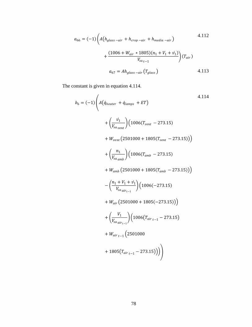
78
𝑎66 = −1 𝐴 𝑔𝑙𝑎𝑠𝑠 −𝑎𝑖𝑟 + 𝑐𝑟𝑜𝑝 −𝑎𝑖𝑟 + 𝑚𝑒𝑑𝑖𝑎 −𝑎𝑖𝑟
+ 1006 +𝑊𝑎𝑖𝑟 ∗ 1805 𝑛1 + 𝑉1 + 𝑣1
𝑉𝑠𝑎 𝑡−1
𝑇𝑎𝑖𝑟
4.112
𝑎67 = 𝐴𝑔𝑙𝑎𝑠𝑠 −𝑎𝑖𝑟 𝑇𝑔𝑙𝑎𝑠𝑠 4.113
The constant is given in equation 4.114.
𝑏6 = −1 𝐴 𝑞 𝑒𝑎𝑡𝑒𝑟 + 𝑞 𝑙𝑎𝑚𝑝𝑠 + 𝐸𝑇
+ 𝑣1
𝑉𝑠𝑎 𝑣𝑒𝑛𝑡 1006 𝑇𝑣𝑒𝑛𝑡 − 273.15
+𝑊𝑣𝑒𝑛𝑡 2501000 + 1805 𝑇𝑣𝑒𝑛𝑡 − 273.15
+ 𝑛1
𝑉𝑠𝑎 𝑎𝑚𝑏 1006 𝑇𝑎𝑚𝑏 − 273.15
+𝑊𝑎𝑚𝑏 2501000 + 1805 𝑇𝑎𝑚𝑏 − 273.15
− 𝑛1 + 𝑉1 + 𝑣1
𝑉𝑠𝑎 𝑎𝑖𝑟𝑡−1
1006 −273.15
+𝑊𝑎𝑖𝑟 2501000 + 1805 −273.15
+ 𝑉1
𝑉𝑠𝑎 𝑎𝑖𝑟𝑡−1
1006 𝑇𝑎𝑖𝑟 𝑡−1− 273.15
+𝑊𝑎𝑖𝑟 𝑡−1 2501000
+ 1805 𝑇𝑎𝑖𝑟 𝑡−1− 273.15
4.114

79
Greenhouse Glass Layer:
The new eighth and final layer of the unshaded model is the greenhouse glass.
It is different from the shaded version in that it now has radiative exchange with the
crop canopy and the medium surface. The equation describing the flux of energy in, is
described in equation 4.115, the flux of energy out in equation 4.116, and the storage
of energy in equation 4.117.
𝑓𝑙𝑢𝑥 𝑖𝑛 = 𝐴 𝑔𝑙𝑎𝑠𝑠 −𝑎𝑚𝑏𝑖𝑒𝑛𝑡 𝑇𝑎𝑚𝑏𝑖𝑒𝑛𝑡 − 𝑇𝑔𝑙𝑎𝑠𝑠
+ 1− 𝜌𝑐 𝜃𝑠 𝜏𝛼𝑔𝑙𝑎𝑠𝑠
+ 4휀𝑔𝑙𝑎𝑠𝑠 𝜍 𝑇𝑔𝑙𝑎𝑠𝑠 + 𝑇𝑠𝑘𝑦
2
3
𝑇𝑠𝑘𝑦 − 𝑇𝑔𝑙𝑎𝑠𝑠
4.115
𝑓𝑙𝑢𝑥 𝑜𝑢𝑡 = 𝐴 𝑔𝑙𝑎𝑠𝑠 −𝑎𝑖𝑟 𝑇𝑔𝑙𝑎𝑠𝑠 − 𝑇𝑎𝑖𝑟
+ 4𝐿𝐴𝐼휀𝑐𝑟𝑜𝑝 𝜍 𝑇𝑔𝑙𝑎𝑠𝑠 + 𝑇𝑐𝑟𝑜𝑝
2
3
𝑇𝑔𝑙𝑎𝑠𝑠
− 𝑇𝑐𝑟𝑜𝑝
+ 4 1
− 𝐿𝐴𝐼 휀𝑚𝑒𝑑𝑖𝑎 𝜍 𝑇𝑠𝑢𝑟𝑓𝑎𝑐𝑒 + 𝑇𝑔𝑙𝑎𝑠𝑠
2
3
𝑇𝑔𝑙𝑎𝑠𝑠
− 𝑇𝑠𝑢𝑟𝑓𝑎𝑐𝑒
4.116
𝑠𝑡𝑜𝑟𝑎𝑔𝑒 = 0 4.117
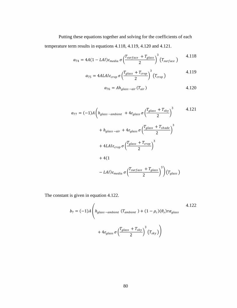
80
Putting these equations together and solving for the coefficients of each
temperature term results in equations 4.118, 4.119, 4.120 and 4.121.
𝑎74 = 4𝐴 1− 𝐿𝐴𝐼 휀𝑚𝑒𝑑𝑖𝑎 𝜍
𝑇𝑠𝑢𝑟𝑓𝑎𝑐𝑒 + 𝑇𝑔𝑙𝑎𝑠𝑠
2
3
𝑇𝑠𝑢𝑟𝑓𝑎𝑐𝑒 4.118
𝑎75 = 4𝐴𝐿𝐴𝐼휀𝑐𝑟𝑜𝑝 𝜍 𝑇𝑔𝑙𝑎𝑠𝑠 + 𝑇𝑐𝑟𝑜𝑝
2
3
𝑇𝑐𝑟𝑜𝑝 4.119
𝑎76 = 𝐴𝑔𝑙𝑎𝑠𝑠 −𝑎𝑖𝑟 𝑇𝑎𝑖𝑟
4.120
𝑎77 = −1 𝐴 𝑔𝑙𝑎𝑠𝑠 −𝑎𝑚𝑏𝑖𝑒𝑛𝑡 + 4휀𝑔𝑙𝑎𝑠𝑠 𝜍
𝑇𝑔𝑙𝑎𝑠𝑠 + 𝑇𝑠𝑘𝑦
2
3
+ 𝑔𝑙𝑎𝑠𝑠 −𝑎𝑖𝑟 + 4휀𝑔𝑙𝑎𝑠𝑠 𝜍 𝑇𝑔𝑙𝑎𝑠𝑠 + 𝑇𝑠𝑎𝑑𝑒
2
3
+ 4𝐿𝐴𝐼휀𝑐𝑟𝑜𝑝 𝜍 𝑇𝑔𝑙𝑎𝑠𝑠 + 𝑇𝑐𝑟𝑜𝑝
2
3
+ 4 1
− 𝐿𝐴𝐼 휀𝑚𝑒𝑑𝑖𝑎 𝜍 𝑇𝑠𝑢𝑟𝑓𝑎𝑐𝑒 + 𝑇𝑔𝑙𝑎𝑠𝑠
2
3
𝑇𝑔𝑙𝑎𝑠𝑠
4.121
The constant is given in equation 4.122.
𝑏7 = −1 𝐴 𝑔𝑙𝑎𝑠𝑠 −𝑎𝑚𝑏𝑖𝑒𝑛𝑡 𝑇𝑎𝑚𝑏𝑖𝑒𝑛𝑡 + 1− 𝜌𝑐 𝜃𝑠 𝜏𝛼𝑔𝑙𝑎𝑠𝑠
+ 4휀𝑔𝑙𝑎𝑠𝑠 𝜍 𝑇𝑔𝑙𝑎𝑠𝑠 + 𝑇𝑠𝑘𝑦
2
3
𝑇𝑠𝑘𝑦
4.122

81
4.3.3 Greenhouse Controls:
Heating/venting
To generalize the model, the heating and venting capacities of the greenhouse
model are based on the area of the greenhouse. The heating capacity of the model
greenhouse was determined through the recommended standards of the ASABE
(2006). Heaters are sized such that when the outdoor temperature is at the 99% winter
design dry bulb temperature, the setpoint of the greenhouse can be maintained, with no
solar input. The equation to determine the heater capacity is made up of losses due to
radiation, conduction and convection, and through infiltration, neglecting losses
through the floor and around the perimeter:
𝑞𝑒𝑎𝑡𝑒𝑟 = 𝑈𝐴𝑐 𝑡𝑖 − 𝑡0 + 1800𝑉𝑁 𝑡𝑖 − 𝑡0 4.123
where: U is the approximate overall, heat transfer coefficient (W m-2
C-1
)
Ac is the area of the greenhouse cover (m2)
ti is the greenhouse air temperature (C)
to is the outside air temperature (C)
1800 is the assumed specific heat of air (J m-3
C-1
)
V is the volume of the greenhouse (m3)
N is the infiltration rate (air exchanges per second) (s-1
)
Typical values for these parameters are available in the ASABE standards. Assuming
single sealed glass, U is 6.2 W m-2
K-1
, 1 hectare floor area greenhouse, Ac is 12500
m2, ti is 24C, to is -15.8 C (ASHRAE 2009, Binghampton, NY value), V is 3.0E4 m
3,
N is 2.8E-4 s-1
due to well maintained glass, the total heat input required to match the
load is 3.68E6 W. If we divide this number by the area this corresponds to a heating
capacity of 1327 kJ m-2
hr-1
(370 W m-2
).

82
Venting capacity can be estimated from the equation:
1 − 𝐸 𝜏𝐼𝐴𝑓 = 𝑈𝐴𝑐 𝑡𝑖 − 𝑡0 + 𝑄𝑣𝐴𝑓𝑐𝑝𝑒𝑥
𝑉𝑒𝑥 𝑡𝑖 − 𝑡𝑖𝑛𝑙𝑒𝑡
4.124
where: E is the evapotranspiration coefficient
η is the solar transmissivity of the greenhouse
I is the solar radiation, (W m-2
)
Af is the floor area (m2)
Vex is the specific volume of the air leaving the greenhouse (m3 kg
-1)
Qv is the ventilation rate (m3 s
-1 m
-2)
cpex is the specific heat of the air leaving the greenhouse (J kg-1
C-1
)
tinlet is the temperature of air entering the greenhouse (C)
Following the guidelines of the ASABE standards, values for these parameters can be
estimated. Assuming a value of 0.5 for E, 0.7 for η (standards suggest 0.88, but that is
for glass alone, not the entire greenhouse structure (Albright, personal
communication)), for η, 900 W m-2
for I for the July 21st solar noon, 1.0E4 for Af, 30C
for ti, 0.8695 m3 kg
-1 for Vex, 1006 J kg
-1 C
-1 for cpex, 28.0 C for to (from the 1%
cooling DB temperature for Binghampton, NY), and 23.1 C for tinlet (assuming the
temperature immediately inside the cooling pads is 2.0C higher than the Mean
Coincident Wetbulb Temperature from the 1% MCWB for Binghampton, NY of 21.1
C) results in a ventilation rate (Qv) of 0.0375 m3 s
-1 m
-2 (135 m
3 h
-1 m
-2).
The calculation to determine the amount of heating and/or venting occurring
during the simulated hour was based on a user defined air temperature setpoint, with a
tolerance of 0.1 K. The simulation was then run with the maximum heating rate. If
the resulting predicted air temperature was below the setpoint minus the tolerance, the
maximum heating value was kept, as the heating/cooling setting. If the predicted air
temperature was above the setpoint minus the tolerance, the simulation was run with

83
maximum venting. If the resulting predicted air temperature was above the setpoint
plus the tolerance, the maximum venting rate was kept as the heating/cooling setting.
If the predicted air temperature was below the setpoint plus the tolerance, it was
determined that the setpoint temperature was within the ability of the system to
achieve. To determine whether heating or cooling is required, the simulation was run
with no heating or venting. If the predicted temperature was above the setpoint, then
venting was required; below the setpoint, heating. To determine the correct heating
(or venting) setting, a bisection search was used. The bisection algorithm was run
until the achieved predicted temperature was within the setpoint +/- the tolerance.
Pad cooling
In the summer time, when keeping the greenhouse cool enough is not possible
through venting with ambient air alone, evaporative cooling is enabled. The air drawn
into the greenhouse for venting purposes is first passed through a pad saturated with
water. The air causes some of the water to evaporate, increasing the humidity ratio of
the air. However, the enthalpy of the air remains almost the same, which means the
air temperature is decreased. A process efficiency of 0.75 was assumed. The new dry
bulb temperature resulting is given by equation 4.125.
𝑇𝑑𝑏𝑛𝑒𝑤 = 𝑇𝑑𝑏 − 𝑇𝑑𝑏 − 𝑇𝑤𝑏 휀𝑝𝑎𝑑 4.125
where: Tdb is the dry bulb temperature (K)
Twb is the wet bulb temperature (K)
εpad is the process efficiency
For a well functioning cooling pad the process efficiency εpad is assumed to be 0.75.

84
The new humidity ratio for the air is
𝑊𝑛𝑒𝑤
= 2501.0− 2.381 𝑇𝑤𝑏 − 273.15 𝑊𝑠𝑎𝑡 − 𝑇𝑑𝑏𝑛𝑒𝑤 − 273.15 + 𝑇𝑤𝑏 − 273.15
2501.0 + 1.805 𝑇𝑑𝑏𝑛𝑒𝑤 − 273.15 − 4.186 𝑇𝑤𝑏 − 273.15
4.126
where: Wsat is the saturation humidity ratio
The remainder of the properties of the air can be calculated from these two values.
The cooling pads are only used for certain months of the year, and the decision
to employ them is made by the grower. To simplify this decision the simulation
model assumes cooling pads are in use when the outside drybulb air temperature is
greater than 20C. This decision is made on an hourly basis, though in reality a grower
usually only decides whether or not to use the cooling pads on a daily or longer basis.
Lighting and shading
The control of supplemental lighting and shading was simulated according to
the LASSI (Light And Shade System Implementation) algorithm described in Albright
(1996). It is a control algorithm to optimize the cost of providing a constant daily light
integral. The decision timeframe for the algorithm is on an hourly basis which
matches the simulation time-step.
Outside of the LASSI implementation, the shades were closed during the night
to conserve energy. Shades were automatically closed in the hour after sunset occurs,
and opened in the hour before sunrise is predicted.
To simulate the heat load, and light output of supplemental lighting, the
number of luminaires m-2
was taken from a commercial greenhouse located in Dryden,
NY (Albright personal communication). In this greenhouse, 146 high pressure sodium
luminaires at 675 W each (including ballast) light 595 m2 (6400 ft
2). This provides a

85
light level of 180 µmols PPF m-2
s-1
. Assuming the lights are 20% efficient 4.77E5 J
m-2
hr-1
of heat is transferred to the greenhouse air, and 1.19E5 J m-2
hr-1
, is transferred
as radiation to the crop and medium.
Nutrient solution temperature control
If the nutrient solution temperature is to be set at a fixed temperature, as in the
case of modeling nutrient solution temperature control, the assumption is made that
nutrient solution temperature has a negligible effect on the air and crop temperatures.
This assumption allows use of the same greenhouse climate data set for nutrient
solution temperature control, as in the uncontrolled condition (though the values of the
nutrient solution are set at the specified target). The assumption implies that nutrient
solution cooling equipment is sized to be able to handle the cooling load under any
conditions.
4.3.4 Input to the model and initial conditions:
The ambient environmental conditions which constitute the input to the model,
are the outdoor dry bulb temperature, the relative humidity, and the solar irradiation.
The data set for the model was collected at the Game Farm Road station, at Cornell
University in Ithaca, NY over the course of twelve years from 1985 to 1996. The
original data files consisted of the year, month, day and hour, and the corresponding
temperature in F, relative humidity in %, and solar irradiation in BTU ft-2
. The
program automatically converts the units of temperature to C, and solar irradiation to
W m-2
. The original 12 data files were combined into a single text file containing all
the information, to facilitate the running of the program.
Initial conditions for the greenhouse model were generated by running the
program using 1988 data with a deep soil temperature of 9.88 C (49.8 F) which is the
average air temperature for the years 1985 to 1997. The values on December 31st, 11

86
pm, were then set as the initial temperatures. It was felt that any major divergence
between the crop and air temperatures, which change quickly in response to climate
conditions, is outweighed by the subsequent more typical values of soil, concrete,
pond and medium temperatures which are slower to respond to changes in outdoor
climate.
4.3.5 Implementation of Greenhouse model
The greenhouse simulation model was coded in Java. The JAMA package was
imported to facilitate solving of the matrices. Input and output files were encoded as
tab delimited text files. Computer code is presented in Appendix A.
4.4 RESULTS:
4.4.1 Model testing
Steady State
To determine if the equations of the model have been input correctly and the
system behaves as expected, steady state testing was used. Setting the initial
temperature of all layers and the boundary conditions to the same temperature of 24C,
and disabling all heat inputs such as the heating/cooling system, the pump and natural
and supplemental light, should result in all layers maintaining their initial temperatures
if the equations and signs of all terms are input correctly. The results of this test are
plotted in Figure 4.2.
If the sign of a term was reversed it would result in a net gain (or loss) of
energy in a particular layer which would then translate into a change in temperature
within that and surrounding layers. Because the temperatures remain the same as their
initial value, no such reversal is present in the equations.

87
Figure 4.2 Model temperatures with a common initial temperature and no heat
inputs/outputs.
Step Input
To determine if the equations correctly predict the direction of heat flow, and
that parameter values for the convective, radiative and conductive heat transfer
coefficients are reasonable, a step input test was used. By setting the initial
temperature of a particular layer higher (or lower) than the rest of the layers, an energy
imbalance is introduced. Differences in temperature (energy) drive heat flow, and so
the model should seek to balance the level of energy within all the layers through heat
transfer.
Figure 4.3 is a plot of the temperatures of the layers over the course of 200
hours, when the initial temperature of the pond was 35C, and the remaining layers,
24C.
0
5
10
15
20
25
30
t_so
il
t_co
ncr
ete
t_w
ater
t_m
edia
t_su
rfac
e
t_cr
op
t_ai
r1
t_sh
ade
t_ai
r2
t_gla
ss
Tem
per
atu
re (
C)
time = 0 hrs
time = 10 hrs

88
Figure 4.3 Temperatures of the greenhouse simulation model layers as a function of
time when the initial temperature of the pond is set to 35C and the remaining layers to
24C.
As expected the temperature in the pond only drops from 35C as there are no
further energy inputs to the model. The concrete (because of its relatively large
thermal mass) is slower to respond to the temperature change than the other layers, but
eventually does, and then closely follows the temperature of the pond. The soil with
an even larger thermal mass, barely responds at all. The medium and the medium
surface are quick to respond to the temperature difference and also closely follow one
another. The greenhouse air in greenhouse airspace 1 and 2, the shade and the
greenhouse glass are also quick to respond to the energy input and follow the same
trend as one another, however, the farther removed from the pond water layer, the less
the response. All layers tend to approach the initial temperature of 24C, as the extra
energy within the pond water layer is dispersed to the other layers.
22
24
26
28
30
32
34
36
0 50 100 150 200
Tem
per
atu
re (
C)
Time (hr)
t_soil
t_concrete
t_water
t_media
t_surface
t_crop
t_air1
t_shade
t_air2
t_glass

89
Heating and Cooling
To test the functionality of the heating and cooling simulation systems it was
necessary to use real environment data for the ambient conditions outside the
greenhouse. The data used was collected in 1988 from the Northeast Climate Center
weather station located on Game Farm Road near Ithaca, NY. 1988 data was used as
that was the dataset with the fewest incidences of missing or incomplete data. Figure
4.4 illustrates the effect of the greenhouse heating system on the greenhouse air during
a typical cold dark winter day. The controlled air temperatures closely follow the
setpoints of 24C during the day and 19C during the night. It is apparent at 7:00 am the
heating system is not quite capable of increasing the temperature within the
greenhouse from the night temperature to the day temperature, though it is close, and
matches real world experience.
The uncontrolled temperatures closely follow the ambient conditions and are
unsuitable for growing spinach. This particular day was quite dark, as there was little
change in temperature during the sunlit hours.
Figure 4.4 Effect of heating (24/19 day/night setpoint) on simulated greenhouse air
temperature during a typical cold, dark winter day.
-10
-5
0
5
10
15
20
25
30
0 5 10 15 20 25Gre
enh
ou
se A
ir T
emp
eratu
re (
C)
Time (hr)
controlled
uncontrolled
ambient

90
Figure 4.5 is a plot of the greenhouse temperatures both with and without the
cooling system functioning on a warm and sunny day.
Figure 4.5 Effect of pad cooling and venting on greenhouse air temperatures (24/19
day/night setpoint) during a typical warm sunny day.
On this particular day the heat gain from solar radiation is quite high and so the
temperature within the unvented greenhouse reaches an unacceptably high temperature
of 41C which also matches real world experience. Venting with evaporative cooling
is quite capable of handling this extra heat load as the day temperature setpoint of 24C
is not exceeded.
4.4.2 Validation of model
Unfortunately there is no readily comparable data with which to compare the
predicted temperatures of the simulation model. The closest commercial facility,
Fingerlakes Fresh (Challenge Industries, Ithaca, NY), collects pond temperatures on a
daily basis, however, this data is of limited use because the ponds are manually heated
0
5
10
15
20
25
30
35
40
45
0 5 10 15 20 25
Air
Tem
per
atu
re (
C)
Time of Day (hr)
No Temperature Control
Temperature Control
Ambient Air

91
in the winter, and cooled in the summer with no associated record of the energy inputs.
According to the temperature logs the ponds are kept at approximately 24C year
round. Figure 4.6 is a plot of the predicted pond temperatures using the 1988 Ithaca
data set.
Figure 4.6 Simulated Pond temperatures over the course of the year using 1988
weather data from Ithaca, NY.
It is possible to examine this plot of temperatures for reasonability. Over the
course of the year there are periods where the pond temperature rises considerably
above the 24 C setpoint of the air temperature within the greenhouse. These periods
of higher temperature occur in the summer when solar heat loads are high. In addition
the pond temperature never drops below the night air temperature setpoint of 19 C.
For the bulk of the year the pond temperature stays within the range of 19 to 24C.
Experience has shown temperatures as high as 27C or so when the pond is not cooled
for awhile. Also of significance is the fact that temperature changes are relatively
18
20
22
24
26
28
30
0 50 100 150 200 250 300 350 400
Tem
per
atu
re (
C)
Day of Year (day)

92
slow; certainly slower than the temperature changes of the greenhouse air. The largest
changes are only on the order of a few degrees over the course of several days.
The temperatures are also similar to the published range of 27 (summer) and
17 (winter) that Bates and Stanghellini (1984) encountered in Arizona in their
commercial spinach pond study.
4.5 DISCUSSION:
The temperature of the nutrient solution has been identified as a key aspect of
the development of Pythium infections in hydroponic baby spinach production. To
simulate the growth and development of both a spinach crop and Pythium infection it
is essential a greenhouse model includes a prediction of the nutrient solution
temperature. Another key aspect of Pythium infections is the time that spinach crops
spend in the nutrient solution before they are harvested, and infected roots removed. It
is also necessary that a greenhouse simulation model includes modern environmental
controls, particularly lighting and shading, as the amount of light a crop receives
dictates its size at harvest time.
The developed lumped parameter, step wise steady state model incorporates
lighting and shading control in addition to the necessary heating and cooling controls
present in commercial greenhouses located in the Northeastern United States. Using
the solar radiation, drybulb temperature and relative humidity as input, the model
predicts on an hourly basis, the temperature of the nutrient solution, and other
temperatures within the greenhouse. Though no data is available to validate the
predictions of the model directly, functionality and reasonability checks on the output
of the model have shown the results are consistent with expectations.
The predicted nutrient solution temperatures respond to the change of season
and roughly mimic temperatures encountered in other commercial greenhouse

93
settings. An important feature of the response is that temperature changes of the
nutrient solution are slow due to the relatively large thermal mass of the pond.
The absolute accuracy of the model is also of lesser importance because of the
eventual use of the model. The results of the model are to be used in a Monte-Carlo
style simulation of various spinach production systems in the presence of Pythium
aphanidermatum. To limit the effects of the greenhouse simulation model on the final
results of the Monte-Carlo simulation, the greenhouse simulation model will be used
to generate a common output that will be used for all of the Monte-Carlo runs. Any
error due to the greenhouse simulation will be common to the results of the Monte-
Carlo simulation.
Careful recording of the energy inputs used to heat and cool the nutrient
solution in a commercial setting would allow a more rigorous validation of the model
in the future. Such a model could then be modified to calculate the energy required to
maintain pond temperatures under a variety of environmental conditions. These
estimations would prove a valuable tool in sizing pond heating and cooling systems.
94
CHAPTER 5: SPINACH GROWTH MODEL
5.1 INTRODUCTION:
To simulate the production of hydroponic spinach, a commonly used growth
model SUCROS (Simple Universal CROp growth Simulator) (Goudriaan and van
Laar, 1994) was adapted for controlled environment conditions.
SUCROS was originally developed at Waginengen University in The
Netherlands (Spitters et al. 1989) as a means of describing crop growth as a function
of the main processes of CO2 assimilation and respiration as they are influenced by
environmental conditions. Alternative approaches to crop modeling using regression
modeling, rely on large sets of data with many different conditions, to accurately
predict crop growth (Spitters 1990). SUCROS, or another similar mechanistic based
model, is useful for modification and use in crop disease work since real-world data
incorporating disease, environmental conditions and crop stage for use in a regression
model would be impractical to obtain, and limited in use.
In his dissertation, Both (1995) modified SUCROS for use in predicting yield
of a lettuce variety grown in controlled environment conditions. The original
SUCROS model was originally developed from crops grown outdoors, not in the
controlled conditions of a commercial greenhouse. Both also looked at supplemental
light and natural light within the greenhouse environment and CO2 as a means of
achieving growth targets, which required further modification of the model as the
original assumed ambient CO2 concentrations, and natural lighting only.
SUCROS relies on a number of parameters to describe the growth and partition
of assimilates into the roots and shoot (leaf and stem). Some of these parameters can
be generalized from other crops, while others are more specific to spinach. The values
of these parameters can be found by applying the model to real world data already
collected to study the growth of hydroponic baby leaf spinach. Such data was

95
collected both as a part of the original NYSERDA spinach project, and also during the
subsequent NYSERDA spinach disease study. From this data and the developed
parameters, the SUCROS framework can be used to describe the growth and
development of a spinach crop. Because the crop to be harvested is babyleaf spinach
only vegetative growth needs to be considered. The crop is harvested before energy is
put into reproductive structures, which would change the growth of the organs of
commercial interest, namely the leaves.
The objectives of this chapter are to:
1. adapt the modified SUCROS growth model developed by Both, to an hourly
basis,
2. develop the parameters necessary to describe hourly baby leaf spinach growth,
from literature values,
3. use actual growth data/measured values to provide the parameters unavailable
from the literature,
4. use actual growth data to validate the model.
5.2 LITERATURE REVIEW:
There are many options available for modeling the growth of a particular crop.
Simple regression analyses can allow the estimation of crop yields based on
environmental inputs such as light and temperature. However, a major drawback
associated with these types of models is that they require the data used to develop the
regression parameters vary over the range for which the model is expected to be valid.
To acquire such data would require a prohibitive number of experiments under
varying conditions.
Another form of crop modeling is the mechanistic approach. This form of
model seeks to predict yields based on the underlying physical processes that drive it.

96
These types of models are more complicated in nature and, overall, predictive
accuracy may suffer due to the many parameters used, each of which may have its
own level of inaccuracy. However many of the parameter values can be found in the
literature either for a specific crop, or as a general value for C3 or C4 photosynthesis.
In addition, the conditions within a greenhouse are usually held within a tightly
controlled range, and are not subject to the large seasonal variations that an outdoor
crop faces. This is an important consideration as the resulting model should not be
used to predict results for situations that are far outside the range of conditions used to
develop the model.
For the spinach growth model it was decided a mechanistic model would be
best suited for the purposes of modeling the growth of the crop under the conditions of
damage done by Pythium aphanidermatum. A mechanistic model offers the
opportunity to directly modify the parameters affecting growth due to Pythium
damage; this modification would not be as meaningful/applicable in a regression type
model. The mechanistic model is also more suitable for making calculations on an
hourly basis.
Many mechanistic models have been developed, but one of the most popular is
the Simple and Universal CROp growth Simulator (SUCROS) (Spitters et al. 1989).
SUCROS functions by determining crop growth based on processes such as CO2
assimilation, light interception, respiration and assimilate partitioning. The model
itself is made up of several submodels, each used to describe some process of growth.
Many of the parameters necessary for the model can be found or adapted from the
literature, or determined experimentally.
SUCROS simulates the dry matter accumulation (growth) of the crop by
partitioning the carbohydrates produced through photosynthesis into what is required
for maintenance (respiration), and what is available for plant growth. The

97
carbohydrates available for crop growth are then partitioned into the roots/shoot, of
which the stem portion is further divided into that going to the stem and that to the
leaves. Baby spinach is harvested very early in its growth cycle when growth is
strictly vegetative; it is not necessary to allocate carbohydrates to reproductive
structures such as flowers and seeds. To determine the amount of carbohydrate
available for distribution throughout the plant, SUCROS calculates the CO2
assimilation rate, which is dependent on the PAR (Photosynthetically Active
Radiation) intercepted by the canopy. This assimilation rate in turn is a function of the
light intensity/characteristics (direct and diffuse) and the leaf area of the crop.
The original SUCROS model was developed to describe growth in field
conditions which are obviously quite different from those encountered in controlled
environment agriculture. In his dissertation, Both (1995) modified the SUCROS
model to account for supplemental lighting and CO2 enrichment. Another factor
affecting the interception of light by the crop is the greenhouse structure itself. The
transmittance of the greenhouse glass (which varies with the angle of the sun) and
structure is also accounted for in Both‟s modifications.
5.3 METHODS AND MATERIALS:
During the original NYSERDA funded spinach production project (Albright et
al. 2005) an experiment was conducted to collect growth data for the purposes of
developing a model to help predict optimal harvest times under specific environmental
conditions previously selected as optimal. This experiment consisted of growing a
spinach crop and harvesting a number of rows of plants every two days. The
harvested material was then weighed, and the leaf area measured. A subsample of the
harvest was used to obtain the dry matter content. Root to shoot ratio was measured
for new seedlings and plants at final harvest by removing the plug of medium the

98
individual plant was growing in, along with the roots. The shoot was removed and
placed in a bag for dry mass measurements while the medium was rinsed from the
roots which were also bagged for dry mass measure.
5.3.1 Spinach Growth Experiments:
Facilities:
The experiment was conducted in a single section of greenhouse (section 15A
of the Kenneth Post Greenhouse complex on the Cornell University Ithaca campus)
from December 4th
, 2004 to December 20th
, 2004. This section of greenhouse
measures 8.5 m by 10.7 m with an eave height of 2.2 m and a roof slope of 25 degrees.
It is covered with glass with an estimated structural light transmittance of 0.7 at
midday. Supplemental lighting was provided by an array of 21 HPS (high pressure
sodium) luminaires arranged to provide a uniform 180 µmols m-2
s-1
of PAR at the
crop height of 1.1 m above the floor.
The crop was grown in two blue plastic ponds (1.2 m * 2 m) with a depth of
0.3 m, containing standard half-strength Hoaglands nutrient solution. The sides and
bottom of the ponds were insulated with 0.07m of polyurethane foam insulation.
Circulation of the nutrient solution was achieved with a 1/20 hp centrifugal pump.
The crop was grown in Styrofoam “Speedling” style floats, which were divided into
26 rows with 13 cells per row. Spinach (cv. Alrite) was seeded into Rediearth®
medium at a moisture content of 3:1 (water to medium by weight) and allowed to
germinate 48 hours at 25 C in a darkened growth chamber. At the time of floating, the
seedling emergence percentage was measured and corrected to provide the same
number of plants per float. Approximately 75% of the cells contained viable plants
after the thinning, resulting in a plant density of 1200 plants m-2
.

99
The air temperature of the greenhouse compartment averaged 23.0 C (sd 0.44)
day/night over the course of the experiment. Solution temperature was not
continuously measured or recorded, but typically follows air temperature closely,
particularly at the time of year the experiment was conducted. Electroconductivity
was maintained at 1200 µS cm-1
and pH 5.8. Measurements and corrections of the
solution were made every two days. Daily light integral over the course of the
experiment averaged 19.3 Mol m-2
day-1
(sd 1.47).
Harvests:
Harvesting of two rows of plants per pond started two days after floatation
when rows 1 and 2 were harvested. At this stage of growth the plants were small and
edge effects due to plant interactions were felt to be negligible. Four days after
floatation, rows 3 and 4 were harvested. At six days after floatation the plants were
beginning to interact with each other, so three rows were harvested. The exposed row
acted as a guard row, which was not used for measurements. The use of a guard row
continued until the final harvest 16 days after floatation. Immediately upon cutting,
the fresh weight for each plant was measured, recorded and placed in a labeled brown
paper bag. Following harvest, the leaf areas of the cotyledons and true leaves were
measured and recorded. After leaf area measurements the plants were placed back in
their bags and placed in a drying oven at 70 C. After 72 hours, they were removed
from their bags and weighed to determine dry mass. This procedure was done in both
ponds at the same time to provide a comparison between ponds.
The ratio of root to shoot was determined by selecting 10 plants from a float
and removing entire individual plants (shoots and roots) along with their medium.
The shoots were removed and bulked into paper bags for dry weight measurement.
The roots were rinsed to remove the medium and also bulked into a different paper

100
bags for dry weight measurement. This procedure was carried out on three different
flats at both the time the crop was originally floated, and at final harvest.
5.3.2 Adaptation of SUCROS to baby spinach growth:
The original SUCROS model by Spitters (Spitters et al. 1989) was developed
for wheat and was adapted by Both (1995) for greenhouse production of lettuce. A
major modification from the original SUCROS and Both‟s verison is the time step
used for the model. When modeling crops such as wheat in outdoor conditions the
growth cycle is longer than the relatively quick sixteen day crop cycle used to produce
baby leaf spinach. To account for the addition of supplemental lighting, the
controlled conditions in greenhouses and the short crop cycle of baby leaf spinach, it
was decided to shorten the time step from one day to one hour. This time step also
corresponds to the time step used in the greenhouse climate simulation model, the time
step used in supplemental light and shading decisions, as well as to the frequency of
most climatic data collection.
Many of the parameters to describe growth can be extended from the wheat
(original SUCROS) and lettuce (Both version of SUCROS) to spinach; however some
adaptation of their values was necessary to more closely fit the growth curves
observed in the baby spinach growth experiment detailed previously. Data from pond
one were used to develop the parameters used in the model, and the results of the
model compared to the data from pond two.
Equations for the SUCROS growth model are not presented in this text unless
they were modified. The equations can be found in Appendix A, the computer coding
of the model; however, a more detailed explanation and derivation of these equations
is presented in Goudriaan and van Laar (1994). The values of parameters required for

101
the model are presented in the following sections, along with a justification for their
selection. The parameters are summarized in Table 5.1.
Table 5.1 Symbols and definitions of parameters and variables used in the modified
SUCROS hourly spinach growth model.
η Greenhouse transmittance
A Coefficient relating leaf mass to Leaf Area Index
AMX Maximum CO2 assimilation rate (kg CO2 ha-1
hr-1
)
DAYL Length of day (sunrise to sunset) (hr)
DEC Declination angle of the sun (radians)
DOY Day of the year
DSINB daily integral of the sine of solar inclination (s day-1
)
DSINBE Daily integral of SINB with a correction for lower atmospheric
transmission at lower solar elevations (s day-1
)
DTGA Daily gross crop CO2 assimilation (kg CO2 ha-1
d-1
)
EFF Initial light conversion factor for individual leaves (kg CO2 ha-1
leaf h-
1)/(J m
-2 s
-1)
FRDF Fraction of radiation that is diffuse
FLV Fraction of photosynthate diverted to leaves
FRT Fraction of photosynthate diverted to roots
FSH Fraction of photosynthate diverted to shoot
FST Fraction of photosynthate diverted to stem
Hd Average diffuse radiation (W m-2
)
Hday Daily light integral outside the atmosphere (W m-2
)
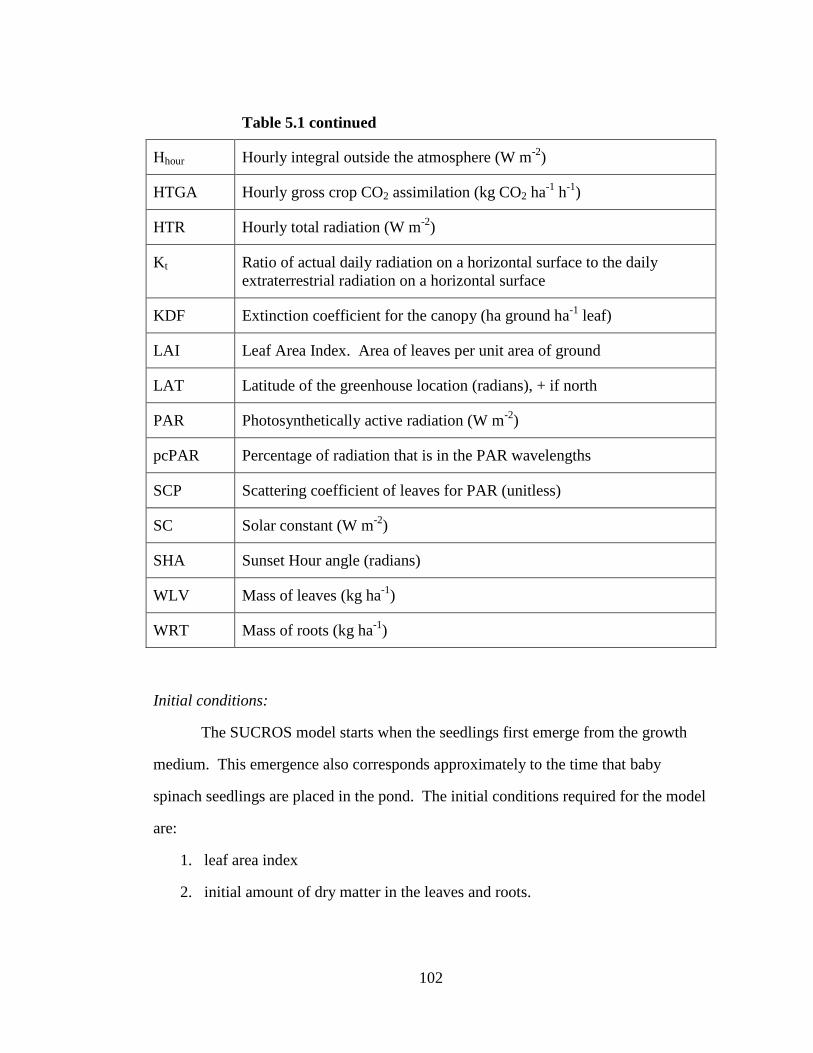
102
Table 5.1 continued
Hhour Hourly integral outside the atmosphere (W m-2
)
HTGA Hourly gross crop CO2 assimilation (kg CO2 ha-1
h-1
)
HTR Hourly total radiation (W m-2
)
Kt Ratio of actual daily radiation on a horizontal surface to the daily
extraterrestrial radiation on a horizontal surface
KDF Extinction coefficient for the canopy (ha ground ha-1
leaf)
LAI Leaf Area Index. Area of leaves per unit area of ground
LAT Latitude of the greenhouse location (radians), + if north
PAR Photosynthetically active radiation (W m-2
)
pcPAR Percentage of radiation that is in the PAR wavelengths
SCP Scattering coefficient of leaves for PAR (unitless)
SC Solar constant (W m-2
)
SHA Sunset Hour angle (radians)
WLV Mass of leaves (kg ha-1
)
WRT Mass of roots (kg ha-1
)
Initial conditions:
The SUCROS model starts when the seedlings first emerge from the growth
medium. This emergence also corresponds approximately to the time that baby
spinach seedlings are placed in the pond. The initial conditions required for the model
are:
1. leaf area index
2. initial amount of dry matter in the leaves and roots.

103
These values were determined through experimental measurement of a newly emerged
crop. The typical planting density used in experiments was approximately 1200 plants
m-2
. The leaf area index at time of floating is approximately 0.1 (ha leaf ha-1
ground);
the initial dry matter in the leaves is approximately 33 kg leaf ha-1
, and roots 5 kg
roots ha-1
.
Crop Development:
Because we are concerned with a babyleaf product, determination of the
developmental stage of the crop is unnecessary. The crop always stays in a vegetative
growth state, which makes the development stage and development rate unneeded in
this model.
Leaf CO2 assimilation:
Leaf CO2 assimilation rate is another parameter that is affected by temperature.
The maximum value (AMX) at light saturation is 40 kg CO2 ha-1
hr-1
at ambient CO2
concentrations. Following Goudrian and van Laar (1994) the CO2 assimilation rate
(AMAX) linearly increases from 0 to 100% of the maximum value for temperatures
from 0 to 10 C, is 100% of the maximum value from 10 to 25 C, and then linearly
decreases from 100% to 0% for temperatures from 25 to 35 C.
Daily Gross CO2 assimilation
The original SUCROS model determined the daily gross crop CO2 assimilation
(DTGA), but because the spinach model is hourly, an hourly gross crop CO2
assimilation (HTGA, kg CO2 ha-1
h-1
) was used. The gross CO2 assimilation is
determined from the amount of PAR intercepted by the crop (J m-2
s-1
) canopy and the

104
CO2 assimilation/light response of the individual leaves. Three parameters are used in
the assimilation/light response of the leaves, EFF, KDF and SCP.
1. EFF is the initial light conversion factor for individual leaves (kg CO2 ha-1
leaf
h-1
)/(J m-2
s-1
)).
2. KDF is the extinction coefficient for the canopy (ha ground ha-1
leaf).
3. SCP is the scattering coefficient of leaves for PAR (unitless).
For ambient CO2 concentrations (which is what is assumed in this model) a typical
value of EFF is 0.45 kg CO2 ha-1
h-1
per J m-2
s-1
. Both (1995) used this value in his
model for lettuce growth. 0.45 is also the value in the original SUCROS model for
wheat, and the value selected for this baby spinach model.
The extinction coefficient for leaves (KDF) suggested in the original SUCROS
model for wheat is 0.6 ha ground ha-1
leaf. Both (1995) used a value of 0.72 for
lettuce. Monteith (1969) tabulated several values of KDF for several different species,
and categorized crop foliage as either planophile or erectophile; planophile canopies
are more evenly spread out, while erectophile canopies tend to be more upright and
potentially clustered closely around the plant stem. The value of KDF is primarily a
function of the angle of the leaves to the incident radiation (which is why there is the
distinction between planophile and erectophile canopies). Values of KDF ranged from
1.13 for cotton, down to 0.29 for Wimmera ryegrass. Both‟s value of 0.72 for lettuce
is the same value as measured for orchardgrass. Both‟s value for lettuce is for the
entire crop period, at the end of which the lettuce plant has a tightly clustered canopy.
Because the baby spinach plants are grown at a high density, the leaves point upwards
as they do not have the room to spread out. This condition makes the spinach more
like the erectophiles with a low value for KDF. For this reason a value of 0.50, which
is more similar to alfalfa, was selected for spinach.

105
The original SUCROS model, and Both (1995), use a value of 0.2 for the
scattering coefficient of the leaves for PAR (SCP). Monteith (1969) states the
proportions of radiation transmitted and reflected by crop leaves are usually similar.
For this reason a value of 0.2 for SCP is also used for baby spinach.
To determine the amount of PAR available within the greenhouse for the
leaves to use, a series of calculations was conducted. The weather data used by the
model includes outdoor solar radiation. This data must be modified to take into
account losses through the greenhouse glazing, and losses through shading. In
addition the angle of the incident radiation is considered when calculating the amount
and character of PAR (direct or diffuse) at different layers of the canopy. These
calculations followed Both (1995), but were modified for hourly calculation.
The first step is to calculate the solar parameters for the entire day:
5.1
where: DEC is the declination of the sun (radians)
DOY is the day of the year
And intermediate variables:
5.2
5.3
where: LAT is the latitude (radians), + if north.
The daylength (DAYL) in hours is given by equation 5.4:
5.4

106
The daily integral of the sine of solar inclination (DSINB) in s day-1
is:
5.5
The daily integral of SINB with a correction for lower atmospheric
transmission at lower solar elevations (DSINBE) in s day-1
is:
𝐷𝑆𝐼𝑁𝐵= 3600
∗
𝐷𝐴𝑌𝐿 ∗ 𝑆𝐼𝑁𝐿𝐷 + 0.4 ∗ 𝑆𝐼𝑁𝐿𝐷2 + 0.5 ∗ 𝐶𝑂𝑆𝐿𝐷2
+12 ∗ 𝐶𝑂𝑆𝐿𝐷 ∗ 2 + 3 ∗ 0.4 ∗ 𝑆𝐼𝑁𝐿𝐷 ∗ 1−
𝑆𝐼𝑁𝐿𝐷𝐶𝑂𝑆𝐿𝐷
2
𝜋
5.6
The solar constant (SC) (W/m2) corrected for a varying earth-sun distance is:
5.7
These parameters need only be calculated daily. To determine the hourly PAR and the
proportions of PAR which are diffuse and direct, a series of calculations is necessary:
The first step is to determine the proportions of PAR that are diffuse and direct.
In the original SUCROS model and in Both, an average daily value for the fraction
diffuse (FRDF) is used. However, because this model has an hourly basis, it is
necessary to modify the procedure to estimate the fraction diffuse. By comparing the
measured value of total radiation (contained in the weather data file), with the
expected amount of solar radiation outside the atmosphere, it is possible to calculate
this fraction. The first step is to calculate the daily integral outside the atmosphere (W
m-2
):
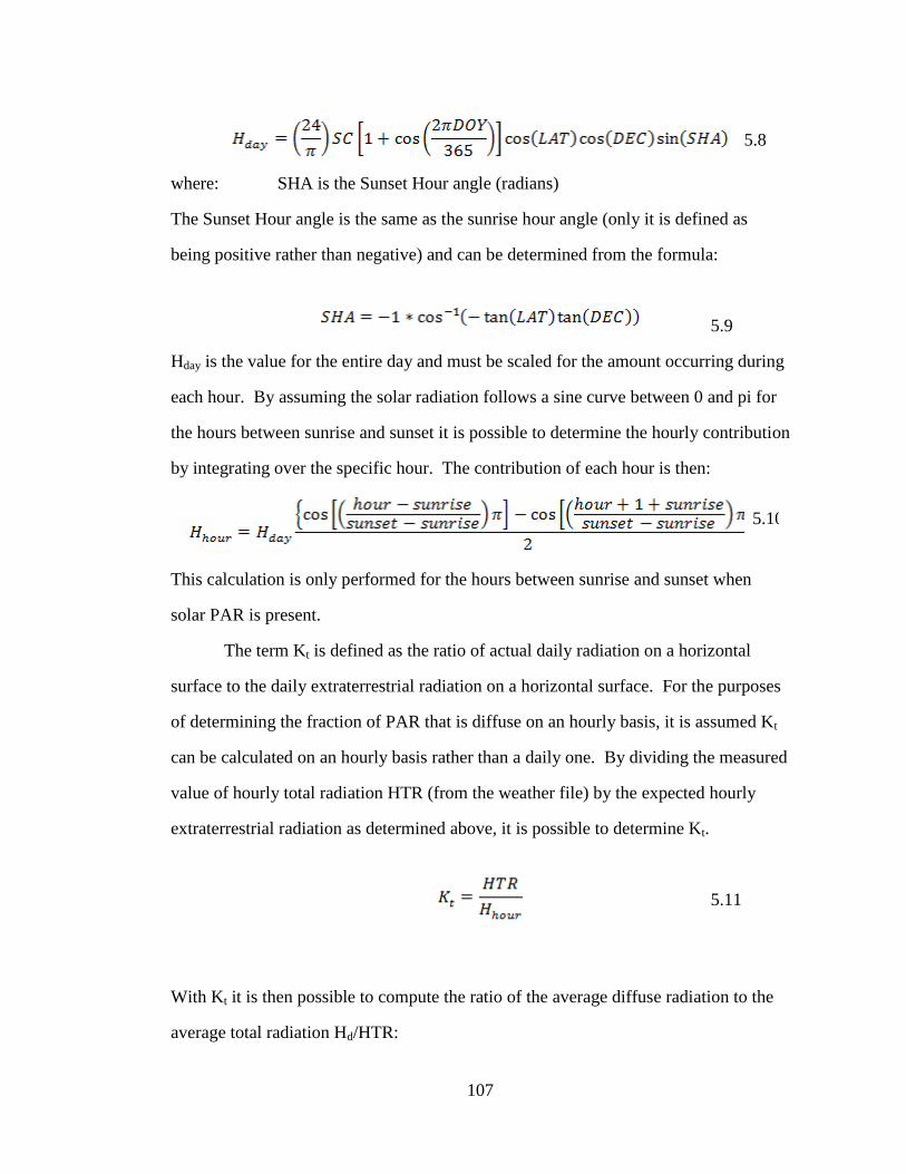
107
5.8
where: SHA is the Sunset Hour angle (radians)
The Sunset Hour angle is the same as the sunrise hour angle (only it is defined as
being positive rather than negative) and can be determined from the formula:
5.9
Hday is the value for the entire day and must be scaled for the amount occurring during
each hour. By assuming the solar radiation follows a sine curve between 0 and pi for
the hours between sunrise and sunset it is possible to determine the hourly contribution
by integrating over the specific hour. The contribution of each hour is then:
5.10
This calculation is only performed for the hours between sunrise and sunset when
solar PAR is present.
The term Kt is defined as the ratio of actual daily radiation on a horizontal
surface to the daily extraterrestrial radiation on a horizontal surface. For the purposes
of determining the fraction of PAR that is diffuse on an hourly basis, it is assumed Kt
can be calculated on an hourly basis rather than a daily one. By dividing the measured
value of hourly total radiation HTR (from the weather file) by the expected hourly
extraterrestrial radiation as determined above, it is possible to determine Kt.
5.11
With Kt it is then possible to compute the ratio of the average diffuse radiation to the
average total radiation Hd/HTR:

108
5.12
The remainder is the direct portion of PAR.
5.13
The amount of solar PAR (direct and diffuse) reaching the crop within the greenhouse
(in J m-2
s-1
) is:
5.14
where: pcPAR is the percentage of radiation that is in the PAR wavelengths
(assumed to be a constant 0.55).
η is the greenhouse transmittance assumed to be a constant 0.7.
HTR is hourly total radiation (J m-2
s-1
)
The remaining procedures and equations used to calculate HTGA are identical to those
used by Both, and the original SUCROS model, with the exception that since gross
assimilation is calculated hourly, there is no need to use a five point Gaussian
approximation to determine daily gross assimilation by calculating hourly gross
assimilation at the five times of day specified by the Gaussian approximation method.
The five point Gaussian approximation is, however, used to calculate the effects of
PAR (diffuse and direct) on the canopy as used in the original models.
Carbohydrate Production:
CO2 is converted to carbohydrate (CH2O) with a ratio of 30/44 (30 being the
molecular weight of carbohydrate, and 44 the molecular weight of CO2. The hourly
production of carbohydrate is then just the hourly gross crop CO2 assimilation rate
(HTGA) multiplied by the ratio 30/44.

109
Maintenance:
Part of the carbohydrate produced is required for maintaining the plant. The
cells within the various plant structures respire and this respiration rate is a function of
temperature. The original SUCROS model uses values of 0.03 (% of mass) for the
leaves, and 0.015 (% of mass) for the roots and stems. Both (1995) also used these
values for lettuce. These values are for daily maintenance and were scaled to an
hourly percentage by dividing by 24.
Dry Matter partitioning:
Carbohydrate production not used for maintenance of the plant is available for
plant growth. The SUCROS model assumes the fractions that describe the distribution
are constant, or else vary as a function of the developmental stage. Because the
spinach growth model is only considering early growth, the distribution factors are not
varied with the crop age.
The excess carbohydrate is first partitioned between the roots and the shoots
(FRT, and FSH). Further partitioning of the shoot portion occurs between the leaves
and the stems (FLV, and FST). To simplify the model, this secondary partitioning
was not used because the entire shoot is harvested, not just the leaf.
To determine the fraction of roots, data from the growth experiments was used.
Observed values at initial floating and at final harvest remained relatively constant
0.162 (stdev 0.03) at floating and 0.163 (stdev 0.4) at harvest. A constant value of
0.16 was assumed for all stages of the crop.
Growth of Plant organs and Translocation:
Once the produced carbohydrates have been partitioned into the various plant
structures, it is possible to estimate the change in dry weight. Different structures

110
have different conversion factors since leaves, stems and storage organs have different
requirements. As baby leaf spinach is an immature plant with negligible stems, we
can consider values for just the leaves and roots. Typical values for leaves are 1.463
kg CH2O required to produce 1 kg dry matter, and 1.444 kg CH2O for the roots
(Goudriaan and van Laar, 1994).
Another simplification that arises due to using a very young crop is we can
ignore translocation from organ to organ which occurs as a plant matures and moves
resources from older, shaded leaves and stems into fruits/other leaves.
Leaf Development:
In the original SUCROS model, Goudrian and van Laar considered the initial
phase of leaf growth to be exponential and temperature limited. Assimilates are not
considered limiting as stores from the seed supplement photosynthesis in the
cotyledons and leaves. According to Goudrian and van Laar this phase lasts until a
leaf area index (LAI) of 0.75 is reached. From the spinach growth experiment a rapid
and non-linear increase in the leaf area of the plants was also observed (Figure 5.1).
The peak LAI reached during the 16 day growing cycle was approximately 15
which is more than the cutoff of 0.75 suggested by the SUCROS model (and in fact at
a level where senescence of lower leaves would normally occur). But the baby
spinach production system is not typical of normal plant growth since the plants are
placed at a density of approximately 1200 per m2 and are not respaced. Because the
crop is to be harvested as a baby product the high leaf area indexes are tolerated.
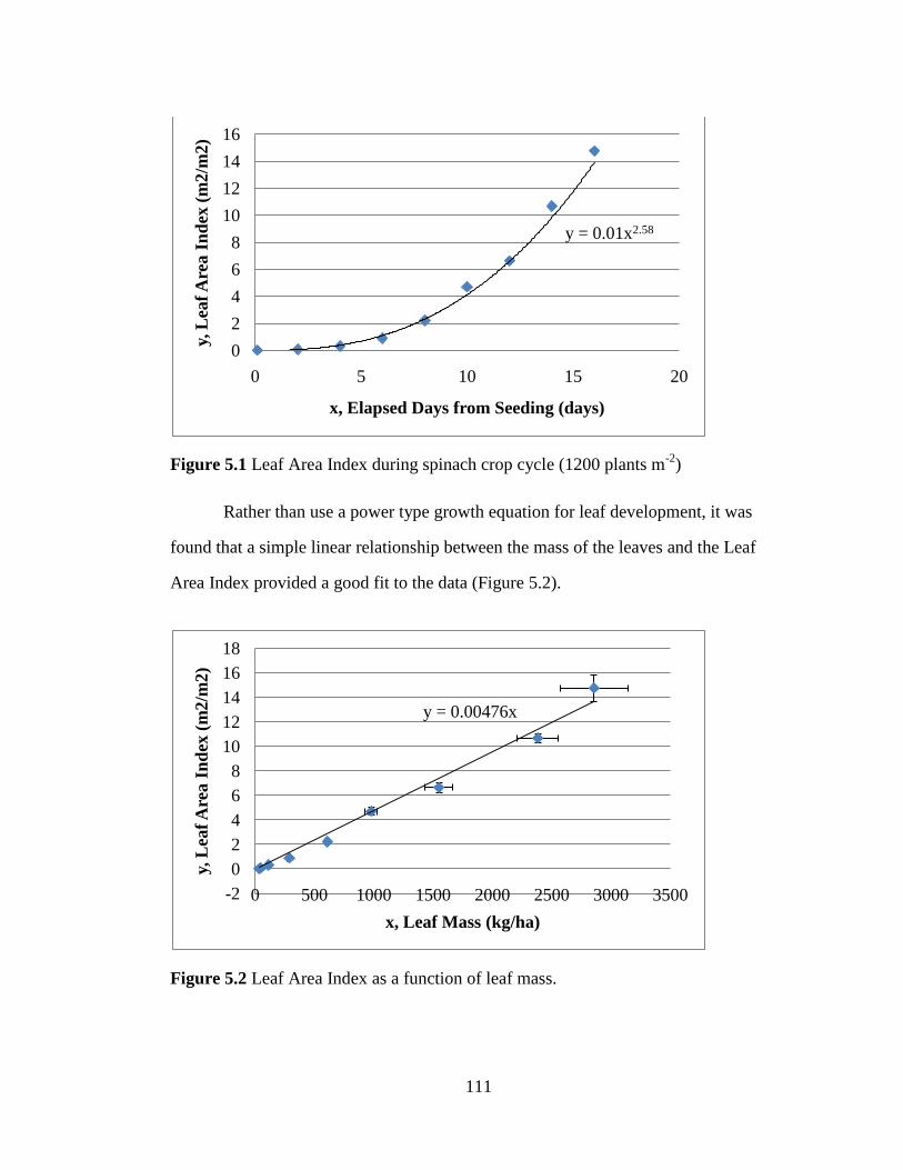
111
Figure 5.1 Leaf Area Index during spinach crop cycle (1200 plants m-2
)
Rather than use a power type growth equation for leaf development, it was
found that a simple linear relationship between the mass of the leaves and the Leaf
Area Index provided a good fit to the data (Figure 5.2).
Figure 5.2 Leaf Area Index as a function of leaf mass.
y = 0.01x2.58
0
2
4
6
8
10
12
14
16
0 5 10 15 20
y, L
eaf
Are
a I
nd
ex (
m2/m
2)
x, Elapsed Days from Seeding (days)
y = 0.00476x
-2
0
2
4
6
8
10
12
14
16
18
0 500 1000 1500 2000 2500 3000 3500
y, L
eaf
Are
a I
nd
ex (
m2/m
2)
x, Leaf Mass (kg/ha)

112
Forcing the intercept of the Leaf Area Index through the origin, the formula relating
Leaf Area Index (LAI, m2 m
-2) to leaf mass (WLV, kg ha
-1) is:
𝐿𝐴𝐼 = 𝐴 ∗𝑊𝐿𝑉 5.15
where A = 0.00476.
Dry matter production:
To determine the total dry weight of each plant organ (and the entire plant as
well), the individual growth rates are multiplied by the integration period (timestep, 1
hour) and then added to their previous dry weights of plant organs. As done
previously, the methods of the original SUCROS, and Both, models were followed
with the exception that calculations were hourly rather than daily. During times of day
when no photosynthesis is occurring, a loss of biomass occurs as maintenance costs
are a constant and there is no production of photosynthate to overcome these losses.
5.3.3 Implementation of the modified SUCROS model:
The SUCROS model was implemented as a series of functions programmed in
Java. For each hour of the simulation, the program would follow the same algorithmic
steps as the original SUCROS model.
The controlled environment setpoints of the experiment (air temperature and
target light integrals) were put into the greenhouse simulation model and the
simulation run. Data from the greenhouse simulation model, such as estimated
temperatures and light levels (both solar and supplemental) within the greenhouse,
were saved in data files which provided the input to the crop growth model. Hourly
values of leaf biomass and Leaf Area Index were saved in text files for comparison
with measured data.
A listing of the code used is in Appendix A.
113
5.3.4 Validation of the spinach growth model:
A number of tests were performed to determine the validity of the spinach
growth model. The first test was a direct comparison of the calculated biomass
accumulation with the measured values. Leaf area was not directly compared as the
simulated leaf area is a function of the biomass. This test was performed for the
conditions of the experiment and was also run for daily target integrals of 5 to 25 mols
m-2
(in increments of 5 mols). The second comparison was performed to determine if
the growth of the crop was directly proportional to the amount of light it received, as
suggested by Both et al. (1996). The range of 5 to 25 mols m-2
was selected as what
could be expected within a greenhouse with no supplemental lighting or shade control.
To test the sensitivity of the model to the values of particular parameters, each
of the parameters was varied plus and minus 10% of the original value, and the model
run (with the original values for the remaining parameters). The final biomass
accumulation at harvest as predicted by the model was recorded. The variability in the
final biomass accumulation for each parameter was sorted in a descending manner
(from greatest to least variability) and results plotted in a tornado style plot, to
illustrate which parameters have the greatest effect on the model.
5.4 RESULTS:
5.4.1 Spinach growth experiments:
The crop was successfully grown for the duration of the experiment with no
evidence of root disease or other factors that could potentially negatively affect the
results. Harvest data including leaf area and fresh and dry weights, in addition to
photosynthetically active radiation (PAR) totals are summarized in Table 5.2.

114
Table 5.2 Individual fresh weight, dry weight, leaf area and cumulated PAR totals at
each harvest day during spinach growth experiment.
Days elapsed
from flotation
(d)
Individual Plant n Average Standard
Deviation
PAR
Accumulation
(mol m-2
)
2 Fresh Weight (g) 24 0.027 0.007 38.5
Dry Weight (g) 24 0.003 0.002
Leaf Area (cm2) 24 0.6 0.2
4 Fresh Weight (g) 24 0.104 0.023 78.4
Dry Weight (g) 24 0.008 0.003
Leaf Area (cm2) 24 2.7 0.9
6 Fresh Weight (g) 25 0.296 0.089 116
Dry Weight (g) 25 0.019 0.005
Leaf Area (cm2) 25 7.5 2.5
8 Fresh Weight (g) 30 0.713 0.099 154
Dry Weight (g) 30 0.041 0.006
Leaf Area (cm2) 9 18.4 1.6
10 Fresh Weight (g) 27 1.607 0.270 192.7
Dry Weight (g) 21 0.065 0.015
Leaf Area (cm2) 8 39.1 7.4
12 Fresh Weight (g) 26 2.352 0.578 230.4
Dry Weight (g) 17 0.103 0.032
Leaf Area (cm2) 17 55.3 14.9
14 Fresh Weight (g) 24 3.712 0.985 269.3
Dry Weight (g) 16 0.159 0.047
Leaf Area (cm2) 13 89.0 10.6
16 Fresh Weight (g) 49 4.336 1.745 308.7
Dry Weight (g) 28 0.191 0.101
Leaf Area (cm2) 10 122.9 28.2
5.4.2 Validation of the SUCROS baby spinach growth model
Measurements of leaf area and plant biomass from the growth experiments
were collected based on individual plant measurements which were then extrapolated
based on plant density to a crop sized hectare basis to be compared to the results from
the adapted SUCROS model. Because SUCROS was originally developed for use in
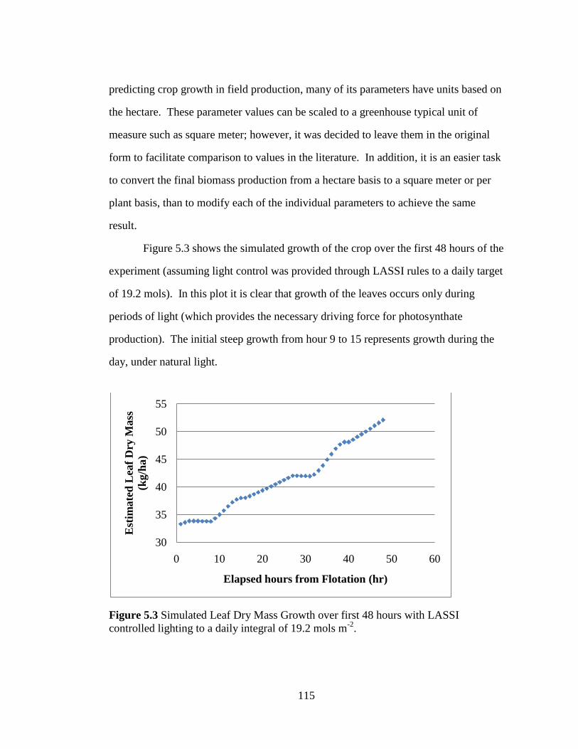
115
predicting crop growth in field production, many of its parameters have units based on
the hectare. These parameter values can be scaled to a greenhouse typical unit of
measure such as square meter; however, it was decided to leave them in the original
form to facilitate comparison to values in the literature. In addition, it is an easier task
to convert the final biomass production from a hectare basis to a square meter or per
plant basis, than to modify each of the individual parameters to achieve the same
result.
Figure 5.3 shows the simulated growth of the crop over the first 48 hours of the
experiment (assuming light control was provided through LASSI rules to a daily target
of 19.2 mols). In this plot it is clear that growth of the leaves occurs only during
periods of light (which provides the necessary driving force for photosynthate
production). The initial steep growth from hour 9 to 15 represents growth during the
day, under natural light.
Figure 5.3 Simulated Leaf Dry Mass Growth over first 48 hours with LASSI
controlled lighting to a daily integral of 19.2 mols m-2
.
30
35
40
45
50
55
0 10 20 30 40 50 60
Est
imate
d L
eaf
Dry
Mass
(kg/h
a)
Elapsed hours from Flotation (hr)

116
After sunset supplemental lighting is applied to meet the target light
requirement; however, this light is applied at a lower rate than natural lighting
(approximately 180 µmols m-2
s-1
). This period is followed by a period of decrease in
the mass of leaves which represents a time when respiration is consuming
photosynthate and none is being produced.
Figure 5.4 is a plot of both the simulated growth and the actual measured
growth from Pond two (Pond one data was used to generate the parameters used in the
model that were not determined from the literature such as relating plant biomass to
the leaf area).
Figure 5.4 Measured and simulated leaf dry mass over the course of the crop cycle.
Grown with 19.2 mol m-2
day-1
PAR.
The model was developed based on growth experiments conducted under a
single daily light integral of 19.2 mols. To determine whether the model scales
production to fit the amount of light received, the model was run with daily light
targets from 5 to 25 Mols. The results are displayed in Table 5.3.
0
500
1000
1500
2000
2500
3000
3500
0 5 10 15 20
Lea
f D
ry M
ass
(k
g/h
a)
Elapsed days from Flotation (d)
Measured
Simulated

117
Table 5.3 Predicted biomass as a function of daily light integral compared to the
baseline 19.2 mols with a production of 2565 kg/Ha at 16 days
DLI Biomass Expected Actual
(mol m-2
) (kg/Ha) (DLI/19.2) (Biomass/2565)
5 592 0.26 0.23
10 1302 0.52 0.51
15 1987 0.78 0.77
20 2682 1.04 1.05
25 3416 1.30 1.33
The model appears to scale very well to the amount of light received by the
crop with a very slight underestimation at low daily integrals and a slight
overestimation at high daily integrals. This verifies the expected linear relationship
between crop growth and light intercepted by the crop, with a range typical of what
might be found in a greenhouse.
To test the sensitivity of the model to the values selected for each parameter
the following parameters were varied ± 10% and the simulated biomass accumulation
on harvest day 16 recorded: AMX, EFF, KDF, SCP, A, MAINLF, and MAINRT. The
results were tabulated, sorted by magnitude and presented in Figure 5.5.
Figure 5.5 Tornado plot of the effect of varying model parameters +/- 10% on the
simulated crop biomass (kg/ha) at harvest day 16.
1500 1700 1900 2100 2300 2500 2700 2900
MAINRT
SCP
MAINLV
AMX
KDF
a
EFF
Crop Biomass at Day 16 (kg/ha)

118
Variables relating to the amount of PAR and the character of the PAR were not
selected for sensitivity testing as they relate to light, to which the model has been
shown to behave in a linear fashion. Though the values of the parameters such as the
transmittance of the greenhouse and the shade curtain, and the percentage of PAR in
solar radiation are estimates, their variability affects the model in a predictable and
linear fashion.
5.5 DISCUSSION:
The SUCROS growth model is a framework that has been used by researchers
to model many different crops. Typically the crops modeled are field crops grown
under natural outdoor conditions. Both (1995) modified this model for greenhouse
production, by adding in the effects of supplemental CO2 and lighting, as well as the
effect of the greenhouse structure on the quantity and quality (diffuse/direct ratio) of
light. However, as in the original SUCROS model, Both was interested in a mature
crop and so the time step he used was one day. To model a fast growing short cycle
crop like hydroponic baby spinach, and to be responsive to the hourly time step of
light control, it was felt a time step of one hour would perform better. The primary
adaptation of the original SUCROS model, and Both‟s version, was to develop the
equations necessary to determine the ratio of diffuse and direct PAR in the
greenhouse. To calculate this ratio a technique was developed (Albright, personal
communication) by which the extrasolar radiation for the hour could be determined by
taking the daily value and scaling it using a sine curve for the daylight hours. Using
hourly measurements it was then possible to use the same equations as used for daily
determination of the diffuse/direct ratio. This technique proved successful and was
ultimately used in the model. Alternatively the individual daily values could have
been calculated using the original technique of the SUCROS model and then the same

119
value used for all hours of the day, but this would potentially overestimate the direct
component in the morning and evening and underestimate it during the middle of the
day. The remaining changes to the SUCROS model were simply a matter of directly
scaling parameter values from daily to hourly. The techniques and equations used
remained the same.
Being a mechanistic model, the backbone of SUCROS is its parameters.
Rather than rely on regression modeling of large data sets (that would be difficult to
obtain for all the conditions of interest) SUCROS uses an understanding of the
processes behind crop growth and development coupled with parameter values that
can either be measured or estimated. The variables used in SUCROS are not solely
for use in SUCROS, rather they are parameters that have been developed over the
years by horticulturalists to better understand and compare how different crops
develop and grow. Unfortunately, the parameter values needed for this particular
growth model were not directly available from the literature, required an
understanding of how they are derived and how the values would change for a crop
harvested before it is fully mature. This selection and adaptation of parameter values
is not ideal, but the alternative of directly measuring values from baby spinach crops
would require special apparatus and measurement techniques, the benefits of which
would be questionable. Especially since the values would then be used in a relatively
imprecise model. In addition, the purpose of developing this model is to facilitate
comparisons between different growing conditions. The accuracy of the end result is
less important than the relative response of the model to differing input.
The parameter developed from observed growth, namely, the relation between
the biomass of the crop and leaf area index, maintained a clear linear relationship
through all ages of the crop. In the original SUCROS model the development stage of
the crop is important, because the characteristics of the plant growth change as the

120
crop matures. For this reason the original SUCROS model uses a more complicated
model to relate biomass to leaf area index and is a function of the development stage.
By focusing on a baby leaf crop, it was possible to simplify the original SUCROS
model and use the observed linear relationship.
As a part of validating the model, biomass growth data from a parallel growing
experiment was compared to the simulated biomass growth. The model has a
tendency to overestimate growth through most of the crop cycle, but underestimate
production in the final few days. This error is most likely due to the values of the
parameters that were determined from the literature, which were taken from other
crops, grown under quite different conditions. The conditions of hydroponic
production are quite different from those encountered in field production. Growth
rates higher than those measured in the field are expected in hydroponics, where
conditions are optimally controlled. An ample supply of water and nutrients, coupled
with temperature and light control, reduce the stress on a crop and allow it to grow
closer to its theoretical optimum.
The scalability of the model due to light is an important property that is
perhaps more valuable than the absolute accuracy of the model. Differences in
variations of spinach varieties could potentially have different responses and
parameter values, resulting in different final harvest weights. However, the ultimate
purpose of this model is to simulate production under varying conditions with the
primary variable being light. Fortunately, this model mimics the linear response to
light integral that has been observed in spinach production.
There are, however, several limits to the use of this model that could
potentially appear in greenhouse production. The model was developed based on a
single plant spacing of approximately 1200 plants m-2
coupled with a harvest at day
16. This spacing was found during previous spinach work (Albright et al., 2005) to be

121
optimal for baby spinach production. Closely related to the spacing is the selection of
the harvest time. At the Cornell university greenhouses, light levels have typically
been controlled to between 15 and 20 mols m-2
per day. These light levels are based
on previous experience with other crops, the Ithaca, NY climate, and the cost of
supplemental lighting. With this amount of lighting (and a density of 1200 plants m-2
)
it was found that harvesting from 12 to 16 days after floatation produced a good crop.
Extrapolating to different spacings would be difficult as this would potentially change
the grow rates of the crop through more or less competition for light. The model was
also not developed for extremes of temperature and humidity. Usually, extremes of
temperature are not a problem in a greenhouse as long as the temperature control
equipment in place, such as heaters, shades and evaporative coolers, are functioning
properly. Some protection from temperature extremes is due to the pond itself, acting
as a temperature buffer. High humidity conditions can be encountered in the winter
months when venting is restricted to conserve energy; however, this parameter is
usually monitored by the control system, and not permitted to reach levels that would
seriously impact crop growth.

122
CHAPTER 6: PYTHIUM APHANIDERMATUM GROWTH AND TRANSMISSION
MODEL
6.1 INTRODUCTION:
In the original description of the SUCROS plant growth model, a major
assumption was the model is for use in conditions where the crop is not limited by
water and nutrients, and not hindered by the presence of pests or disease (Goudriaan
and van Laar, 1994). This condition is not met for the case of modeling the growth of
a crop in the presence of Pythium aphanidermatum, a water borne root mold which
spreads rapidly through the nutrient solution and attacks plant roots. However,
SUCROS is well suited for modification to model the disease interaction, as its
mechanistic form separates individual growth of root and shoot due to photosynthate
production.
In her doctoral dissertation entitled “Influence of Plant Age, Inoculum Dosage,
and Nutrient Solution Temperature on the Development of Pythium aphanidermatum
in hydroponic Spinach (Spinacia Oleracea L.) Production Systems”, Katzman (2003)
documented much of the data necessary to expand the SUCROS growth model to
account for Pythium processes. Reported data include the effects of initial zoospore
concentration in the nutrient solution, time of inoculation and nutrient solution
temperature on root and shoot damage, zoospore concentrations in solution, and
mycelium development. Her data coupled with experiments performed during the
NYSERDA spinach disease project (Albright et al., 2007), forms the basis of the
Pythium growth and transmission model and modification of the SUCROS model.
The developed model was validated by comparing predicted multi-crop cohort growth
and development under disease conditions, to those observed during the NYSERDA
spinach disease project. Continuous production experiments with multiple aged crops
in the same pond were carried out and a part of these studies involved inoculating the

123
multi-cohort system with known concentrations of zoospores and measuring the
growth of the cohorts as the disease progressed. Also during these experiments, an
uninoculated control pond became infected. Data from this condition was used to help
quantify the development of an infection under natural conditions, as would be most
likely to occur in a commercial setting.
The objectives of this chapter are to:
1. develop the framework and parameters for a model to predict the growth and
spread of Pythium aphanidermatum in hydroponic baby spinach production
under controlled environment conditions,
2. modify the SUCROS based baby spinach crop growth model to take into
account the damage done to the crop‟s roots due to Pythium aphanidermatum
zoospores and mycelium,
3. validate the functionality of the model by comparing predicted crop growth
and Pythium disease damage to experimentally collected data.
6.2 LITERATURE REVIEW:
6.2.1 Pythium aphanidermatum lifecycle:
Pythium species are a widespread and major pathogen that affect many
different crops in both field and hydroponic culture and have been identified as one of
the most common and destructive pathogens found in hydroponic systems
(Stanghellini and Rasmussen, 1994). Pythium aphanidermatum was also identified as
the causative agent of the root disease that plagued earlier research into hydroponic
spinach production at Cornell (Katzman 2003).
Pythium species can cause seed rot, seedling damping off, and root rot of most
plants (Agrios 1978), however, spinach is particularly susceptible (Howard et al.

124
1994). As described in Agrios, (1978) Pythium is a type of Peronosporale, which in
turn, is a type of Oomycetes. This fungi has elongated mycelium, produces oospores
as resting spores and zoospores or zoosporangia as asexual spores. The life cycle of a
typical Pythium species is illustrated in Figure 6.1.
Figure 6.1 Disease cycle of Pythium sp. (Agrios 1978).
The primary mode of infection of roots is through zoospores, which possess flagella
and allow them to move through continuous films of water. Shortly after release,
zoospores lose their flagella, encyst and grow a germ tube, which allows them to
infect roots. Spore germ tubes or saporophytic mycelium, come in contact with the
tissue of the host plant either by chance, or because exudates from the plant act as a
chemotropic stimulant, which causes zoospores to move to, or mycelia to grow
towards the plants. It is this mobility which exacerbates the problem of Pythium in

125
hydroponic production. Because the crop is grown in a common nutrient solution
(whether the production system is Nutrient Film Technique or pond) zoospores
quickly disperse through the system infecting roots throughout the entire crop.
Once the germ tubes or saprophytic mycelium come in contact with root
material the fungus enters either through direct penetration or cracks, and further
penetrates the tissue through mechanical pressure and enzymatic dissolution.
Breakdown of the tissue occurs as the fungus grows both through and around the cells
and cellulolytic enzymes digest the cell walls. The fungus consumes the plant cell
substances, using them as both a source of energy and as raw material for its own
growth. Infected tissue decays until only a frail remnant of indigestible material is left
behind with the mycelium.
As infection develops and mycelium spreads through the root, the reproductive
stages of Pythium begin to grow and form sporangia and oospores. Sporangia are the
bodies that release zoospores, whereas, oospores are a hardier form of spore which
tolerate both high and low temperatures as well as low moisture conditions. In field
production oospores allow Pythium to survive harsh winter conditions where there
may be limited plant material available, and temperatures are too cold for the survival
of the mycelium. When conditions are amenable again, oospores develop a
sporangium independent of plant material, and release zoospores. However, this
process is considerably slower than direct production of sporangia from mycelium.
However, the oospore stage of Pythium is still an important consideration in
hydroponic production. Oospores present a means of infecting the hydroponic system
via medium (Katzman 2003) and make cleaning up of a hydroponic system difficult.
With the exception of oospores, the various Pythium stages are relatively fragile and
can be inactivated through a number of commercially available technologies (as
detailed in chapter two).

126
6.2.2 Pythium aphanidermatum in hydroponic systems:
For her dissertation, Katzman (2003) examined a number of factors necessary
to model the impact of a Pythium outbreak on a crop. She examined sources of
inoculum, influence of plant age at time of inoculation on disease development,
relationships between inoculum dosage and disease development, and influence of
nutrient solution temperature on plant growth and disease development. Though the
focus of Katzman‟s work was on more mature spinach plants (as opposed to the baby
leaf spinach of this research) many of her findings are still applicable. The most
important finding of Katzman‟s research is that lethality of Pythium is strongly related
to temperature. By examining spinach crops grown under identical conditions, but
with nutrient solution temperatures of 18C, 24C and 30C respectively, and inoculated
with Pythium at 25 zoos ml-1
, Katzman found crops grown at 18C did not differ
significantly from the uninoculated control crops grown at the same temperature. She
also found crops grown at 24C and 30C suffered a 20% and 70% reduction in shoot
dry mass, respectively. This follows other work, such as Bolton (1980), which
suggests Pythium aphanidermatum has an optimal temperature of 30C. Bates and
Stanghellini (1984) found when nutrient solution temperatures were above 23 C,
Pythium aphanidermatum was the dominant oomycete (as opposed to Pythium
dissotocum whose range was 17 to 22 C). This finding has important implications for
hydroponic spinach production. By reducing the temperature of the nutrient solution,
the time required for the mycelia to develop the sporangia necessary to further spread
the infection is increased. This, in turn, may allow the removal of the root material
before the release of zoospores occurs, provided the crop is grown with a short crop
cycle. Removal before zoospore release prevents new material from becoming
infected, and stops the infective cycle.

127
6.3 METHODS AND MATERIALS:
6.3.1 Disease model Framework
The data for the development of the spinach disease model comes primarily
from Katzman (2003). Throughout her series of experiments on age of plant,
inoculum concentration, and temperature effects on disease development, Katzman
always categorized the condition of the roots. Though the categorization of the roots
into classes was somewhat subjective, the fact that it was carried out consistently in all
of her experiments provides a common method of comparison, and allows the effects
she investigated to be integrated into a common model. A summary of the symbols
and variables used is presented in Table 6.1.
Table 6.1 Summary of variables and symbols used in the Pythium aphanidermatum
growth and transmission model.
αconc Concentration effect intercept
αgrow Mycelial growth rate intercept
αtemp Temperature effect intercept
βconc, Concentration effect slope
βgrow Mycelial growth rate slope
βtemp Temperature effect slope
δroot fraction of the root that is dark brown/black
εmycelium Reference amount of mycelium @ 25 zoos ml-1
(kg ha-1
)
ηphoto Coefficient of Photosynthetic Rate reduction
Amature Maturation age of mycelium (hr)
Arelease Zoospore release age (hr)

128
Table 6.1 continued
c Cohort number
E(C) Concentration adjustment factor
E(T) Temperature adjustment factor
GPHOT Gross photosynthetic production (kg ha-1
)
GPHOTda Gross photosynthetic production, adjusted for disease (kg ha-1
)
gr Mycelium growth rate (kg kg-1
hr-1
)
grb Base growth rate at 24 C (kg kg-1
hr-1
)
grp Mycelium growth rate on a per plant basis (g plant-1
)
mf Final mass of mycelium infected root (kg ha-1
)
m0 Starting Mass of mycelium (kg ha-1
)
mc Mass of zoospore releasing mycelium for each cohort c, (kg)
mequiv Equivalent mass of mycelium added due to zoospores in solution (kg)
n Number of periods over which growth is accrued
nzoos Zoospore release amount (zoos kg-1
)
PRAD Adjustment to gross photosynthetic production as a function of root
damage.
T Temperature (C)
vol Volume of nutrient solution (ml)
URMavg Average mass of root that is uninfected (g plant-1
)
URMavg,kg ha-1 Average amount of infected root (kg ha-1
)
zc Number of zoospores released by each particular cohort (zoos)
Zconc Concentration of zoospores in solution (zoos ml-1
)

129
The basis of the spinach disease model is the growth of mycelium within, or on
the roots of the crop. This process is tracked for each cohort of the crop on an hourly
basis. Each hour the amount of new mycelium growth on each cohort is stored in an
array, which is the size of the age of the oldest mycelium material on the cohort, in
hours. In addition to growth of existing mycelium, zoospores in solution attack
available healthy root material, and the mass of mycelium created is a function of their
concentration in solution.
Mj,k is the mycelium array for each cohort
where: j, (1,2,…,j) is the age of the crop cohort in hours
k, (1,2) k = 1 is the temperature adjusted age of the mycelium
(hr)
k = 2 is the total mass of mycelium of this age (kg)
Equation 6.1 provides us with a means of calculating mycelium mass for the
current hour.
𝑀1,2 = 𝑀𝑗 ,2
𝑗
2∗ 𝑔𝑟 +𝑚𝑒𝑞𝑢𝑖𝑣 , 6.1
All of the mycelium is aged by a temperature adjusted amount to account for the
different developmental and growth rates of mycelium at varying temperature. (The
mycelium, in addition to growing faster, also matures faster with increasing
temperature).
The growth rate is adjusted for temperature in equation 6.2.
𝑔𝑟 = grb ∗ 𝐸 𝑇 6.2
The developmental age of the mycelium is calculated in equation 6.3.
𝑀𝑗 ,1 = 𝑀𝑗−1,1 + 1𝑟 ∗ 𝐸(𝑇) 6.3

130
Based on the age of the mycelium, it is classified into one of two categories
following Katzman (the third root category is white which indicates healthy root).
The mycelium starts out as light brown or gray streaking in the roots until reaching
age Amature when the mycelium turns a darker brown/black color. This stage is later
used to provide a measure of the damage to the root function and the shoot quality.
Each hour the mass of mycelium that is greater than or equal to the zoospore
releasing age, (Arelease) releases zoospores which propagate the infection. The total
number of zoospores released is calculated with equation 6.4.
𝑧𝑐 = 𝑚𝑐 ∗ 𝑛𝑧𝑜𝑜𝑠 6.4
The number of zoospores released by the various cohorts of the crop are then
summed and divided by the volume of the nutrient solution of the particular pond, to
give the concentration of free zoospores in solution in the next hour (equation 6.5).
Zconc = zc𝑐1
vol 6.5
These free zoospores then propagate the infection (provided there is uninfected
root material present). The zoospores infect root material and form a mass of
mycelium which is a function of the concentration of the zoospores in the solution (the
higher the concentration of zoospores in solution, the larger the equivalent mycelium
mass formed on the roots). This equivalent mass is determined with equation 6.6.
𝑚𝑒𝑞𝑢𝑖𝑣 = εmycelium ∗ E(C)
6.6
Damage to the growth of the crop is a function of the level of damage to the
roots. Reduced crop growth is modeled by reducing the amount of photosynthate
produced, described in equation 6.7.
𝐺𝑃𝐻𝑂𝑇𝑑𝑎 = GPHOT ∗ PRAD 6.7

131
The adjustment factor for the gross photosynthetic production is determined as
a function of the percentage of the roots that are infected, in equation 6.8.
PRAD = 1− 𝜂photo ∗ 𝛿𝑟𝑜𝑜𝑡 6.8
Shoot quality is a function of the level of damage to the roots as well.
However, rather than an absolute number, the quality is divided into two categories,
saleable and unsaleable. When the level of root damage reaches a certain point (a
function of the percentage of roots that are light brown/streaked and dark
brown/black) the cohort is classified as unsaleable. The infection is initiated by
assuming a specific amount of mycelium is present on new cohorts, representing
natural infection due to oospores, and residual zoospores/mycelium.
The following sections further detail and expand on the processes outlined
above and discuss how parameter values were estimated. A complete listing of the
computer code developed is in Appendix A.
Growth of Mycelium
The growth of Pythium aphanidermatum mycelium is the basis of the disease
model. This process is linked to the damage caused to the roots, which in turn, affects
the shoot growth and quality. As discussed previously, after infection with a
zoospore, mycelium begins to spread through the root, consuming it as it goes. The
mycelium spreads both up and down the root as much as 21 to 24 mm day-1
(Guo and
Ko 1993). Because the disease model developed for baby spinach is concerned with
whole crop and cohorts within crop relations, infections at the individual root are not
directly considered. This permits the simplification of the mycelium growth to a
relative growth rate, based on the amount of mycelium already present, and the
availability of healthy root material to infect.

132
As a part of her quantification of the extent to which spinach is damaged by
Pythium infection, Katzman (2003) developed a “root rot rating” system and
documented the state of the roots throughout her experiment. The “root rot rating”
system is a categorization of the percentage of the roots falling into three categories
based on physical appearance: white, light brown/streaked with gray, and dark
brown/black. White roots were healthy root material. Light brown/streaked with gray
roots were infected with growing mycelium and range from newly infected material to
a more developed infection. The final stage of dark brown/black roots was the point
where roots were heavily damaged/dead.
To estimate a rate at which mycelium grows and spreads through a root
system, data from Katzman‟s chapter entitled, “Influence of Plant Age at Time of
Inoculation on Development of Disease Caused by Pythium aphanidermatum in
Hydroponic Spinach Production “, was used. Of particular interest are her day 1 and
day 9 (days following sowing) inoculations coupled with her day 9 and day 14
harvests (which correspond to times within the range of the usual 16 day baby spinach
crop cycle. Katzman was not focused on baby spinach and so also conducted
inoculations on days 14 and 21, and harvests on days 21 and 28 which are not of direct
use for this model). The relevant data from Katzman has been summarized in Table
6.2 and Table 6.3. Table 6.2 is a summary of the effect of timing of Pythium
inoculation on shoot dry matter, and Table 6.3, is a summary of the condition of the
roots at the associated harvest times.

133
Table 6.2 Influence of time of inoculation on shoot dry mass of spinach. Means and
standard errors of shoot dry mass of plants inoculated with P. aphanidermatum
zoospores on different days (1, 9, or 14) after sowing and harvested 9, 14, and 21 days
after sowing. (From Katzman)
Mean shoot dry mass (g/plant) and standard error
on harvest day
Inoculation
day (D)
Harvest 9 Harvest 14 Harvest 21
Control 0.01 ± 0.00 0.051 ± 0.003 0.268 ± 0.014
Day-1 0.00 ± 0.00 0.008 ± 0.002 0.032 ± 0.012
Day-9 0.01 ± 0.00 0.061 ± 0.013 0.213 ± 0.051
Day-14 0.01 ± 0.00 0.051 ± 0.003 0.252 ± 0.017
Table 6.3 Percentages (%) of roots within each root rot category (1-4). Spinach plants
were inoculated with P. aphanidermatum zoospores on different days (1, 9, or 14)
after sowing and harvested 9, 14, and 21 days after sowing. (From Katzman)
Treatment Percentage (%) of roots within root rot rating on harvest day
Inoculation
day (D)
Root rot rating Harvest 9 Harvest 14 Harvest 21
Control 1- white 100 100 96.7
2 - light brown/streaked 0 0 3.3
3 - dark brown/black 0 0 0
4 – no root 0 0 0
Day-1 1- white 10.3 12.5 20
2 - light brown/streaked 56.4 10 7.5
3 - dark brown/black 25.6 62.5 57.5
4 – no root 7.7 15 15
Day-9 1- white 100 90 5.1
2 - light brown/streaked 0 10 76.3
3 - dark brown/black 0 0 18.6
4 – no root 0 0 0
Day-14 1- white 100 100 60
2 - light brown/streaked 0 0 36.7
3 - dark brown/black 0 0 3.3
4 – no root 0 0 0

134
In developing a mycelium growth rate it was necessary to make several assumptions:
1. root damage is due to Pythium only,
2. root damage is uniform throughout the cohort,
3. mycelium development is visible in the root as a light brown discoloration
and/or streaking after which it develops into a dark brown/black color,
4. root mass is directly proportional to shoot mass even when the roots are
infected with mycelium, and follows a production rate as described in the
SUCROS based spinach growth model,
5. the mycelium growth rate is only a function of available healthy root for
infection,
6. the ageing of the mycelium for determining developmental stage is only a
function of temperature,
7. Pythium zoospores infect the crop in a single hour. They are released and do
not carry over hour to hour,
8. Pythium zoospores, when released, are uniformly spread throughout the pond.
Other organisms and mechanical damage can cause browning of the roots to
some extent. This additional damage complicates the use of root damage as a measure
of the level of mycelium present. However, to simplify the model it was assumed
these contributions are minor. In Katzman‟s uninoculated control condition, after 21
days 3% of the root mass showed some damage, though it was not present in previous
harvests on days 9 and 14. (This small amount of damage was thought to be due to
unintentional Pythium infection).
Another simplification is to assume root damage caused by Pythium is
uniformly spread throughout the cohort. This is not always the case when plants are
exposed to high levels of Pythium at a young age when they are particularly
vulnerable and liable to die outright. Moreover, it might happen in the case of an

135
initial infection, where only a single oospore may infect a single root of a single plant,
which subsequently blossoms into a wider infection. However, since commercial
interest is not in individual plants, but in the crop as a whole, averaging the damage
across the entire crop is one way of accounting for this variation. Missing plants due
to death are offset by surviving plants having less competition for light and space.
In her dissertation, Katzman categorized the conditions of the roots. An
assumption is these root conditions also represent stages in the development of
mycelium, and infected root material first progresses from lightbrown/streaked
through to dark brown/black. Initial light brown streaking and graying occurs very
quickly after infection as mycelium grows up the root. As mycelium develops it
consumes root leaving behind only those compounds it cannot degrade such as lignins
(Agrios 1978), darkening the root from its initial healthy white.
The fourth assumption (root mass is proportional to shoot mass) is necessary
because direct measurements of the amount of root material present at the different
harvests are not available. Shoot dry matter production was collected, along with root
rot ratings (percentages of roots falling into four categorical ratings of health), and
percentage containing mycelium. To determine the rate of mycelium development,
the amount of root material as a function of the age of the crop is required, and to
account for the reduced root material due to Pythium damage, the amount of root
material is scaled according to the reduction in shoot mass.
It was assumed that growth rates of the mycelia are only a function of the
availability of uninfected root. Infections in new cohorts with small root systems
proceed slowly as there is not much root to infect. Infections in older plants with
extensive root systems spread faster. Guo and Ko, (1993) published rates of growth of
mycelia with units of mm day-1
. However, as we are dealing with a whole crop, it is
more convenient to work on a mass basis. An overall rate simplifies the problem of

136
spread between adjacent roots, infections occurring at the top or bottom of the root
(i.e. infection running out of places to spread to) and other complications of not using
a mass basis approach.
To simplify the model, the assumption was made that rate of mycelium
development varies only with temperature (increasing at higher temperatures). The
data collected by Katzman in her experiments on inoculation timing and dosage was
conducted at a single temperature, however, further experiments into the effect of
temperature were also carried out by her in a separate chapter and were used to
develop the relationship between mycelium ageing and temperature.
The basis for assuming that Pythium zoospores cause infections within the
hour they are released is that zoospores are relatively short lived and will tend to
rapidly infect available root material. The swimming stage only lasts approximately
30 minutes (Endo and Colt, 1974), after which the zoospores encyst and are unable to
actively migrate towards roots. In floating pond hydroponics where the density of
plants is great and the volume of nutrient solution relatively small, it is likely
zoospores do not have to travel far before finding available roots to infect.
Using the same root to shoot ratio that was measured as a part of obtaining the
data for the SUCROS spinach model (0.15) it is possible to estimate the root mass per
plant from the measured shoot dry mass (Table 6.2). Then using the root quality data
(Table 6.3) it is possible to estimate the amount of root that is infected with Pythium
mycelium (Table 6.4).

137
Table 6.4 Estimated influence of time of inoculation on mycelium infected root mass
(g plant-1
) of spinach based on measured shoot dry mass values, estimated root growth,
and observed root condition. (Measured values from Katzman)
Innoculation
time
Harvest
Day 9
Harvest
Day 14
Harvest
Day 21
control measured shoot dry mass (g plant-1
) 0.01 0.051 0.268
estimated root mass (g plant-1
) 0.0015 0.00765 0.0402
% root uninfected 100 100 96.7
estimated mass infected (g plant-1
) 0 0 0.00133
Day 1 measured shoot dry mass (g plant-1
) 0.00157 0.008 0.032
estimated root mass (g plant-1
) 0.0002355* 0.0012 0.0048
% root uninfected 10.3 12.5 20
estimated mass infected (g plant-1
) 0.00021 0.00105 0.00384
Day 9 measured shoot dry mass (g plant-1
) 0.01 0.061 0.213
estimated root mass (g plant-1
) 0.0015 0.00915 0.03195
% root uninfected 100 90 5.1
estimated mass infected (g plant-1
) 0 0.00092 0.03032
Day 14 measured shoot dry mass (g plant-1
) 0.01 0.051 0.252
estimated root mass (g plant-1
) 0.0015 0.00765 0.0378
% root uninfected 100 100 60
estimated mass infected (g plant-1
) 0 0 0.01512
*Estimated root mass for the day 1 inoculated material harvested on day 9 is based on the
same ratio as the day 1 inoculated material harvested on day 14. This ratio remained
approximately the same for the harvest 21 and 28 data as well.
Assuming a constant growth rate of the form:
𝑚𝑓 = m0(1 + 𝑔𝑟𝑏)^𝑛 6.9
The growth rate (grb) can be determined by rearranging equation 6.9 to:
𝑔𝑟𝑏 = 𝑚𝑓
𝑚0
1𝑛− 1 6.10
Examining harvests on days 14 and 21 of the material inoculated on day 9, the
estimated mass of infected roots increased from 0.00092 g plant-1
to 0.03032 g plant-1
over the course of the 168 hours between harvests. Using these values in equation

138
6.10 results in a growth rate of 0.021 g g-1
hr-1
. The day 1 inoculated material has an
estimated infected root mass of 0.00021 g plant-1
, on day 9, and 0.00105 g plant-1
on
day 14, using equation 6.10 with 120 hours between harvests; a growth rate of 0.0135
g g-1
hr-1
. On day 21 the day 1 inoculated material has an estimated infected root mass
of 0.00384 g plant-1
. With the 168 hours between harvests this corresponds to a
growth rate of only 0.007 g g-1
hr-1
. The growth rate determined from the day 9
inoculation material is up to three times as large as that from the day 1 inoculation.
However, the day 9 inoculation material was an infection spreading through a large
established root system, whereas, the day 1 inoculation material was constrained by
the lower availability of infectable root. To account for the increasing difficulty in
finding new material to infect the mycelium growth rate was plotted vs. the average
mass of uninfected root as illustrated in Figure 6.2.
Figure 6.2 Mycelium growth rate as a function of the average uninfected root mass.
y = 2.1446x + 0.0101
0
0.005
0.01
0.015
0.02
0.025
0 0.001 0.002 0.003 0.004 0.005 0.006
Myce
lial
Gro
wth
Rate
(g g
-1h
r-1)
Average Uninfected Root mass (g plant-1)
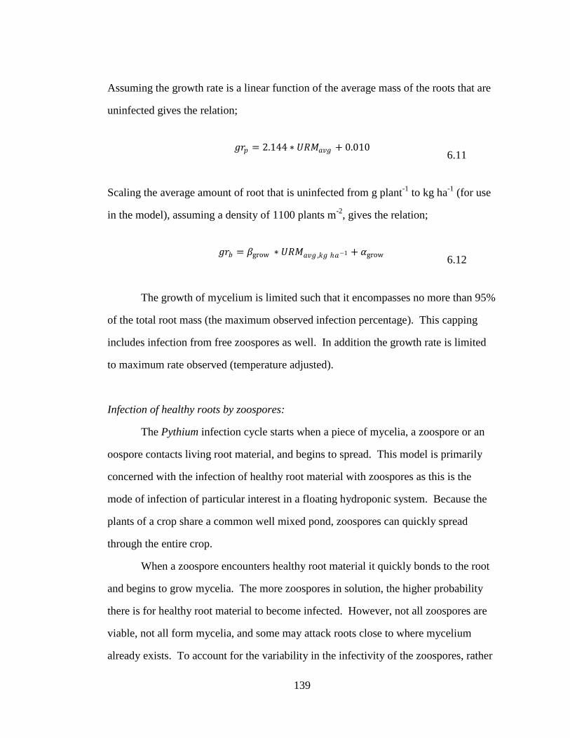
139
Assuming the growth rate is a linear function of the average mass of the roots that are
uninfected gives the relation;
𝑔𝑟𝑝 = 2.144 ∗ 𝑈𝑅𝑀𝑎𝑣𝑔 + 0.010
6.11
Scaling the average amount of root that is uninfected from g plant-1
to kg ha-1
(for use
in the model), assuming a density of 1100 plants m-2
, gives the relation;
𝑔𝑟𝑏 = 𝛽grow ∗ 𝑈𝑅𝑀𝑎𝑣𝑔 ,𝑘𝑔 𝑎−1 + 𝛼grow
6.12
The growth of mycelium is limited such that it encompasses no more than 95%
of the total root mass (the maximum observed infection percentage). This capping
includes infection from free zoospores as well. In addition the growth rate is limited
to maximum rate observed (temperature adjusted).
Infection of healthy roots by zoospores:
The Pythium infection cycle starts when a piece of mycelia, a zoospore or an
oospore contacts living root material, and begins to spread. This model is primarily
concerned with the infection of healthy root material with zoospores as this is the
mode of infection of particular interest in a floating hydroponic system. Because the
plants of a crop share a common well mixed pond, zoospores can quickly spread
through the entire crop.
When a zoospore encounters healthy root material it quickly bonds to the root
and begins to grow mycelia. The more zoospores in solution, the higher probability
there is for healthy root material to become infected. However, not all zoospores are
viable, not all form mycelia, and some may attack roots close to where mycelium
already exists. To account for the variability in the infectivity of the zoospores, rather
140
than consider an absolute number of infections, a specific mass of healthy root is said
to be infected. This mass is assumed to be a function of the concentration of the
zoospores in solution and is limited by the available mass of healthy root to infect.
Using the mycelium growth rate determined previously and rearranging
equation 6.10 to solve for the starting mass of mycelia, the equivalent mass of mycelia
the infecting zoospores create in the roots can be calculated using equation 6.13.
휀mycelium = 𝑚0 =mf
1 + gr n 6.13
The equivalent mass of mycelium can be estimated from three starting points;
day 1 inoculated material, day 9 inoculated material and day 14 inoculated material.
From Table 6.4, plants inoculated on day 9 and harvested on day 14, developed a
mycelium mass of 9.2E-4 g plant-1
, over the course of 120 hours. Assuming a
mycelium growth rate of 0.0105 g g-1
hr-1
(determined from equation 6.10), gives a
starting mycelium mass of 2.42E-4 g plant-1
. Plants inoculated on day 14 and
harvested on day 21, developed a mycelium mass of 0.0151 g plant-1
, over the course
of 168 hours. Assuming a growth rate of 0.0204 g g-1
hr-1
, gives a starting mycelium
mass of 5.06E-4 g plant-1
. Material inoculated on day 1 and harvested on day 9
developed a mycelium mass of 2.1E-4 g plant-1
, over the course of 216 hours.
Because the starting mass of roots is not known, the lowest mycelium growth rate of
0.010 g g-1
hr-1
was assumed. This growth rate corresponds to a starting mycelium
mass of 5.88E-5 g plant-1
. Averaging these three values results in a reference
equivalent mass of mycelium of 2.69E-5 g plant-1
, or 3.23 kg ha-1
, when the
concentration of zoospores is 25 zoos ml-1
.
141
Damage to Crop
The basis for determining the effectiveness of root function and quality of
shoot material is both the quantity and characteristics of damage to the roots. Previous
sections have dealt with determination of growth and spread of mycelium which is
primarily a quantity issue, i.e. the amount of the root infected. In her quantification of
root damage, Katzman categorized roots according to their appearance. Besides the
undamaged categorization she further broke the infected category down into roots that
have light brown/gray streaking, and those that are dark brown/black. The light brown
streaking corresponds to a recent mycelium infection of the roots, which eventually
matures into dark brown/black root material. The presence of dark brown/black root
material usually signified severe damage to the crop and significant biomass
reductions. The presence of light brown streaking did not always correspond to a
reduction in biomass of the plant. For this reason estimating when damaged root
material matures into the dark brown/black stage provides a means to estimate both
the quality and reduction in growth of the shoot.
It is assumed that maturation of root damage is strictly a function of the age of
the mycelium, and is not a response to external triggers such as temperature changes
or other stresses put on the mycelium.
To estimate the age at which mycelium matures into the dark brown/black
stage (Amature), data from Katzman‟s time of inoculation experiment was used. It was
necessary to make the assumption the dark brown/black stage is the final condition of
the mycelium. In addition it was also assumed the “no root” category of Katzman also
belongs to this final condition (essentially dead root material). Examining the day 9
inoculated material, on harvest day 14, 10 percent of the root is in the light
brown/streaked stage. Seven days later on harvest day 21, 76.3 percent of the root was
light brown/streaked and 18.6 percent was dark brown/black. By inserting values of

142
mycelium maturation age into the mycelium growth model in trial and error fashion it
was found a mycelium maturation age of 128 hours (~5.3 days) produced a fraction of
roots dark brown/black of 0.186.
By attacking roots, Pythium aphanidermatum, reduces the ability of the crop to
acquire water and nutrients necessary for normal plant function. Symptoms range
from little to no reduction in growth, to complete death of the plant, depending upon
the extent of the infection. Examining tables 6.1 and 6.2 which are shoot dry mass and
root rot ratings for Katzman‟s time of inoculation experiment, it is apparent shoot
biomass accumulation is only significantly impacted when root damage is heavy.
To reflect the effects of the infection, production of photosynthate by the
leaves, can be decreased as a function of root damage. Reduced photosynthate
production corresponds to less energy and building blocks for crop functions such as
maintenance and new growth.
To scale the photosynthate production it was assumed the presence of infected
root material decreased photosynthate production in a linear fashion.
𝑃𝑅𝐴𝐷 = 1− 𝜂𝑝𝑜𝑡𝑜 ∗ 𝛿𝑟𝑜𝑜𝑡 6.14
The value of ηphoto was selected so the sum of the squared differences between
the observed and predicted percent shoot mass was minimized (for the day 1
inoculation harvests on days 14 and 21 and the day 9 inoculation harvest on days 14
and 21. Day 1 inoculation harvest day 9 was not included, as this value was missing
from the observed data). As can be seen in Figure 6.3 this resulted in an ηphoto value of
0.79.

143
Figure 6.3 Sum of the Squared Error of the fraction shoot biomass reduction as a
function of the coefficient of photosynthetic rate reduction (ηphoto).
6.3.2 Adjustment to Mycelium Growth and Development:
Because the temperature of the nutrient solution may not always be 24 C, it
was necessary to scale growth and development of the mycelium as a function of
temperature. In addition, scaling is also required for the amount of mycelium formed
by zoospores attacking roots, as it is unlikely a crop would be exposed to a level of 25
zoospores ml-1
, such as was used to develop the reference infection mass.
Concentration adjustment
As reported in the fourth chapter of Katzman (2003) entitled “Relationship
Between Inoculum-Dosage and Development of Root Rot Caused by Pythium
aphanidermatum in Hydroponic Spinach Production,” she conducted an experiment
where she inoculated ponds of spinach with known concentrations of zoospores and
measured growth of the crop through periodic harvesting at days 9, 14, 21 and 28. In
addition, Katzman also studied time of inoculation, introducing known concentrations
of zoospores 9, 14 and 21 days after floatation. This data forms the basis for
0
0.02
0.04
0.06
0.08
0.1
0.12
0 1 2 3 4 5
SS
E F
ra
cti
on
Sh
oo
t B
iom
ass
Red
ucti
on
Photosynthetic Rate Adjustment Factor (ηphoto)

144
developing a function to relate the concentration of zoospores in solution to the
infection level of the crop roots.
As was the case for the temperature effect, results were more noticeable if the
root rot rating data is used, and if the data at harvest 21 is included. The results of this
experiment are presented in Table 6.5.
Table 6.5 Percentages (%) of roots within each root rot rating (1-3) at harvest.
Spinach plants were inoculated with P. aphanidermatum zoospores (0.025 to 250 per
ml in 10-fold increments) 9 days after seeding and harvested 14, and 21 days after
seeding. (From Katzman)
Treatment Percentage (%) of roots within Root Rot Rating
at harvest
Dosages-
zoospores per
mL
Root Rot Rating Harvest
14
Harvest
21
Control 1- white 100 91.7
2 - light brown/streaked 0 8.3
3 - dark brown/black 0 0
0.025 1- white 96.7 33.9
2 - light brown/streaked 3.4 50.8
3 - dark brown/black 0 15.3
0.25 1- white 94.9 10
2 - light brown/streaked 5.1 56.7
3 - dark brown/black 0 33.3
2.5 1- white 83.3 6.7
2 - light brown/streaked 16.7 76.7
3 - dark brown/black 0 16.7
25 1- white 88.3 0
2 - light brown/streaked 11.7 67.8
3 - dark brown/black 0 32.2
250 1- white 80 2
2 - light brown/streaked 20 59.2
3 - dark brown/black 0 38.8
Unfortunately, there is confounding data when examining the 0.25 and 2.5
zoos ml-1
treatments. The 0.25 zoos ml-1
treatment appears to have as much damage
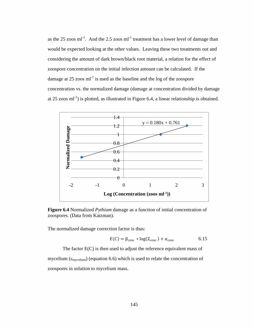
145
as the 25 zoos ml-1
. And the 2.5 zoos ml-1
treatment has a lower level of damage than
would be expected looking at the other values. Leaving these two treatments out and
considering the amount of dark brown/black root material, a relation for the effect of
zoospore concentration on the initial infection amount can be calculated. If the
damage at 25 zoos ml-1
is used as the baseline and the log of the zoospore
concentration vs. the normalized damage (damage at concentration divided by damage
at 25 zoos ml-1
) is plotted, as illustrated in Figure 6.4, a linear relationship is obtained.
Figure 6.4 Normalized Pythium damage as a function of initial concentration of
zoospores. (Data from Katzman).
The normalized damage correction factor is thus:
𝐸(𝐶) = βconc ∗ log Zconc + 𝛼conc 6.15
The factor E(C) is then used to adjust the reference equivalent mass of
mycelium (εmycelium) (equation 6.6) which is used to relate the concentration of
zoospores in solution to mycelium mass.
y = 0.180x + 0.761
0
0.2
0.4
0.6
0.8
1
1.2
1.4
-2 -1 0 1 2 3
Norm
ali
zed
Dam
age
Log (Concentration (zoos ml-1))
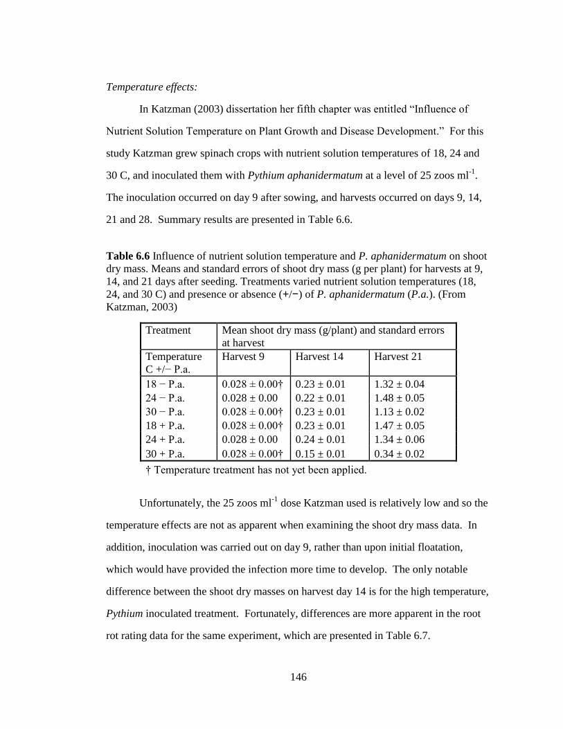
146
Temperature effects:
In Katzman (2003) dissertation her fifth chapter was entitled “Influence of
Nutrient Solution Temperature on Plant Growth and Disease Development.” For this
study Katzman grew spinach crops with nutrient solution temperatures of 18, 24 and
30 C, and inoculated them with Pythium aphanidermatum at a level of 25 zoos ml-1
.
The inoculation occurred on day 9 after sowing, and harvests occurred on days 9, 14,
21 and 28. Summary results are presented in Table 6.6.
Table 6.6 Influence of nutrient solution temperature and P. aphanidermatum on shoot
dry mass. Means and standard errors of shoot dry mass (g per plant) for harvests at 9,
14, and 21 days after seeding. Treatments varied nutrient solution temperatures (18,
24, and 30 C) and presence or absence (+/−) of P. aphanidermatum (P.a.). (From
Katzman, 2003)
Treatment Mean shoot dry mass (g/plant) and standard errors
at harvest
Temperature
C +/− P.a.
Harvest 9 Harvest 14 Harvest 21
18 − P.a. 0.028 ± 0.00† 0.23 ± 0.01 1.32 ± 0.04
24 − P.a. 0.028 ± 0.00 0.22 ± 0.01 1.48 ± 0.05
30 − P.a. 0.028 ± 0.00† 0.23 ± 0.01 1.13 ± 0.02
18 + P.a. 0.028 ± 0.00† 0.23 ± 0.01 1.47 ± 0.05
24 + P.a. 0.028 ± 0.00 0.24 ± 0.01 1.34 ± 0.06
30 + P.a. 0.028 ± 0.00† 0.15 ± 0.01 0.34 ± 0.02
† Temperature treatment has not yet been applied.
Unfortunately, the 25 zoos ml-1
dose Katzman used is relatively low and so the
temperature effects are not as apparent when examining the shoot dry mass data. In
addition, inoculation was carried out on day 9, rather than upon initial floatation,
which would have provided the infection more time to develop. The only notable
difference between the shoot dry masses on harvest day 14 is for the high temperature,
Pythium inoculated treatment. Fortunately, differences are more apparent in the root
rot rating data for the same experiment, which are presented in Table 6.7.

147
Table 6.7 Influence of nutrient solution temperature and inoculation with P.
aphanidermatum on root rot rating (RRR). Percentages (%) of roots within each RRR
category per treatment for plants harvested 14, and 21 days after seeding. Treatments
varied the nutrient solution temperature (18, 24, and 30 C) and presence or absence
(+/-) of P. aphanidermatum (P.a.). (From Katzman)
Treatment Percentage (%) of roots within each RRR
category at harvest day
Temperature C -/+ P.a. RRR Category Harvest
14
Harvest
21
18 C - P.a. 1- white 100 100
2 - light brown/streaked 0 0
3 - dark brown/black 0 0
24 C - P.a. 1- white 100 100
2 - light brown/streaked 0 0
3 - dark brown/black 0 0
30 C - P.a. 1- white 97.6 53.8
2 - light brown/streaked 2.4 44.9
3 - dark brown/black 0 1.3
18 C + P.a. 1- white 100 82.1
2 - light brown/streaked 0 17.9
3 - dark brown/black 0 0
24 C + P.a. 1- white 57.1 6.3
2 - light brown/streaked 42.9 79.7
3 - dark brown/black 0 13.9
30 C + P.a. 1- white 47.6 0
2 - light brown/streaked 21.4 1.3
3 - dark brown/black 31 98.8
In the temperature trials Katzman performed it was clear the amount of root
damage increased as a function of temperature. Katzman also found zoospores were
released from the infected roots earlier in the high temperature conditions. These
observations mean the mycelium grows and matures faster and causes increased
damage by releasing zoospores, which further infect the root. Another assumption to
simplify the temperature effect of the nutrient solution is temperature does not affect
the plant itself. This is not entirely the case as can be seen in Table 6.6, comparing
shoot mass of the uninoculated treatments at harvest day 21. According to this data,

148
there is a penalty for growing at temperatures that are too high. Potentially
exacerbating this effect is the fact the crop might be stressed at higher temperatures,
making it more vulnerable to Pythium damage. The increase in mycelium
development and growth rate at higher temperatures encompasses this effect.
A further assumption is there is no deleterious effect from temperature changes
on the growth of mycelium. Temperatures found in the ponds are within a relatively
constant range and any changes are gradual due to the relatively large volume.
With only three temperatures to use, the mid value of 24C was selected as
baseline (as this was the temperature common to all of Katzman‟s experiments). To
find the adjustment factor for 18C, the conditions of Katzman‟s experiment were used
as input to the model (25 zoos ml-1
inoculated day 9). Through trial and error an
adjustment factor of 0.58 was found to produce the observed 17.9% light
brown/streaking in the roots at harvest day 21. Because it is likely that damage in the
roots at 30C was also partially due to reinfection, this point was not used in the
development of the temperature relation. The 18 and 24 C points are plotted in Figure
6.5.
Figure 6.5 Age adjustment factor as a function of nutrient solution temperature.
y = 0.07x - 0.68
0
0.2
0.4
0.6
0.8
1
1.2
1.4
1.6
0 5 10 15 20 25 30 35Ma
tura
tio
n A
dju
stm
ent
Fact
or
Nutrient Solution Temperature (C)
149
Assuming a linear relation results in:
𝐸 𝑇 = 𝛽temp ∗ 𝑇 − αtemp 6.16
6.3.3 Sources of inoculum
Natural Pythium infections must begin at some point. Usually a few spores
will infect a single plant, and the subsequent release of zoospores will spread the
infection to the rest of the crop. Stanghellini and Rasmussen (1994), identified
growing medium such as peat and sand, along with greenhouse dust and even water
supplies, as potential sources of inoculum. In addition, they found common
greenhouse pests such as shore flies and fungus gnats can potentially transmit Pythium
spores. In her dissertation, Katzman (2003) investigated sources of Pythium
inoculation in the Cornell greenhouse. Potential sources examined included tap and
reverse osmosis supply water, greenhouse medium, and dust, as well as the spinach
seeds themselves. Unfortunately, she was not able to isolate Pythium from any of
these sources. One explanation for this was the number of Pythium propagules was
below her detection limit. Regardless, spontaneous Pythium infections occurred,
confirming that in hydroponic situations, a very small number of Pythium propagules
can quickly mature into a full blown infection.
For the disease model it is necessary to have a starting point to simulate a
spontaneous inoculation. In Katzman‟s various studies she noticed browning of roots
on mature plants always seemed to occur typically at 21 to 25 days after sowing.
Examining the control data in Table 6.2 we can see 21 days after sowing, 3.3% of the
roots were showing signs of the browning associated with Pythium. The experiments
carried out to study the progress and characteristics of infections, relied on dosing with
zoospores at concentrations many orders of magnitude greater than would be expected
for any naturally occurring infection. One option is to assume a set baseline
150
concentration of zoospores are always present (a very low concentration). However, a
problem with this technique is concentration damage relationship developed
previously has an extrapolated lower limit concentration of 0.015 zoospores ml-1
(found by solving equation 6.15 for the zoospore concentration at which the
adjustment factor equals 0).
Another option is to assume the seedlings are already inoculated to a certain
level before they enter the pond, such as would be the case if zoospores/other
infectious material were found in the growing medium. To estimate a value for this
initial mass of mycelia, the developed disease model was used, along with the control
data for Katzman‟s time of inoculation experiment. Using the same conditions
Katzman used (air temperature 24C and 16 mols PAR m-2
day-1
) as input to the growth
and disease model, it was found that a starting mycelial mass of 1.5 E-3 kg mycelium
ha-1
resulted in damage to 3.3% of the roots at day 21, which is the level Katzman
observed. There was no corresponding shoot biomass reduction at this low level of
damage. This starting mass (m0) is thus assumed to exist as a baseline in every new
cohort.
6.3.4 Release of zoospores
Infected roots develop sporangia, which in turn release zoospores. Under
laboratory conditions, the entire reproductive process of Pythium can be as short as 24
hours, zoospore to zoospore, but can take significantly longer in a hydroponic system.
Benchtop evaluations and data from Katzman indicate this reproductive cycle time is
dependent on temperature. In Katzman‟s work, conducted at 24C, she monitored the
level of zoospores present in solution. Unfortunately, her techniques did not allow an
accurate means of measuring these levels, as illustrated by the fact immediately
following inoculation she could not measure the same number of zoospores as were

151
inoculated (Table 6.8). A complicating factor in making such a measurement is that
zoospores actively migrate towards roots and in the relatively root dense environment
of floating hydroponics it is likely that the zoospores released, rapidly find new roots
to infect and are not measured as free zoospores.
Table 6.8 Influence of inoculation time, zoospore concentration and temperature on
zoospores detected in nutrient solution at time of harvest. (From Katzman)
Treatment means and standard errors of zoospores per ml
nutrient solution on harvest day
Experimental
Condition
Harvest 1 Harvest 9 Harvest 14 Harvest 21
Innoculation
Time
day 1 0.87 ± 0.25 0.13 ± 0.03 0.01 ± 0.00 0.04 ± 0.03
day 9 0.99 ± 0.16 0.29 ± 0.02 0.06 ± 0.02
day 14 1.00 ± 0.22 0.09 ± 0.03
day 21 0.82 ± 0.13
Zoospore
conc (zoos
ml-1
)
(innoculated
day 9)
0 0.0 ± 0.0 0.0 ± 0.0 0.0 ± 0.0
0.025 0.0 ± 0.0 0.001 ± 0.001 0.012 ± 0.003
0.25 0.021 ± 0.007 0.004 ± 0.002 0.011± 0.003
2.5 0.165 ± 0.031 0.007 ± 0.005 0.008 ± 0.002
25 1.091 ± 0.115 0.246 ± 0.066 0.067 ± 0.020
250 8.146 ± 1.362 1.269 ± 0.132 0.080 ± 0.011
Temperature
(C)
(innoculated
day 9)
18 3.61 ± 0.18 0.03 ± 0.01 0.00 ± 0.00
24 5.19 ± 0.71 0.01 ± 0.00 0.02 ± 0.01
30 4.72 ± 0.77 0.61 ± 0.21 1.19 ± 0.22
Looking at the day 1 inoculated material, on day 9 it is apparent zoospores are
being released into solution. Encysted zoospores were found to survive up to 7 days
in moist soil conditions (Stanghellini and Burr 1973), but since these zoospores were
detected 9 days after inoculation it is likely they are the results of reproduction from
the original infection. Similarly, with the day 9 through day 21 inoculated material
zoospores were detected after 7 days.
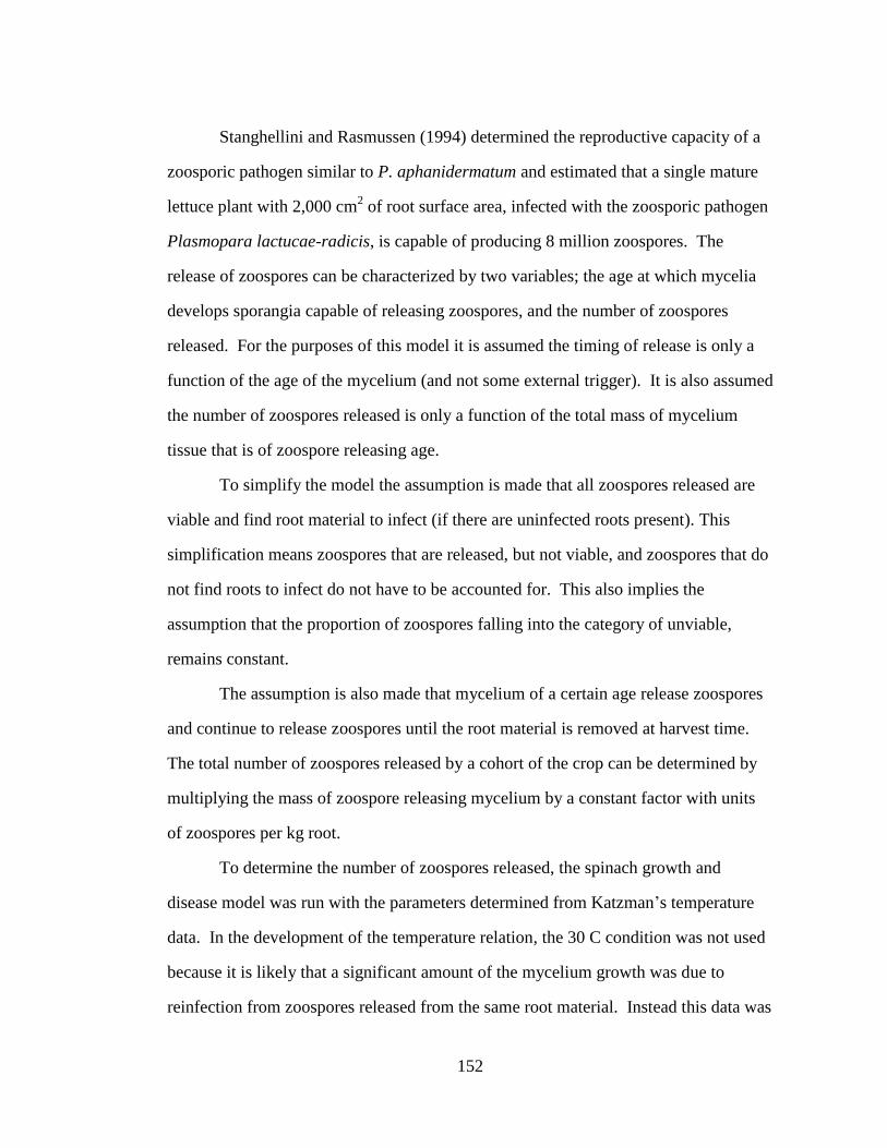
152
Stanghellini and Rasmussen (1994) determined the reproductive capacity of a
zoosporic pathogen similar to P. aphanidermatum and estimated that a single mature
lettuce plant with 2,000 cm2 of root surface area, infected with the zoosporic pathogen
Plasmopara lactucae-radicis, is capable of producing 8 million zoospores. The
release of zoospores can be characterized by two variables; the age at which mycelia
develops sporangia capable of releasing zoospores, and the number of zoospores
released. For the purposes of this model it is assumed the timing of release is only a
function of the age of the mycelium (and not some external trigger). It is also assumed
the number of zoospores released is only a function of the total mass of mycelium
tissue that is of zoospore releasing age.
To simplify the model the assumption is made that all zoospores released are
viable and find root material to infect (if there are uninfected roots present). This
simplification means zoospores that are released, but not viable, and zoospores that do
not find roots to infect do not have to be accounted for. This also implies the
assumption that the proportion of zoospores falling into the category of unviable,
remains constant.
The assumption is also made that mycelium of a certain age release zoospores
and continue to release zoospores until the root material is removed at harvest time.
The total number of zoospores released by a cohort of the crop can be determined by
multiplying the mass of zoospore releasing mycelium by a constant factor with units
of zoospores per kg root.
To determine the number of zoospores released, the spinach growth and
disease model was run with the parameters determined from Katzman‟s temperature
data. In the development of the temperature relation, the 30 C condition was not used
because it is likely that a significant amount of the mycelium growth was due to
reinfection from zoospores released from the same root material. Instead this data was

153
used to determine the zoospore release age and number of zoospores released per kg
of mature mycelium. At 30 C, with no inoculation, 46.2% of the roots were infected
at harvest 21.
In determining the zoospore release age, and the number of zoospores released
per kg of mature mycelium it became apparent these two variables are highly
correlated to one another. By selecting a younger zoospore release age, a smaller
number of zoospores released per kg would produce the 46.2% damage in the roots at
harvest day 21. Similarly an older zoospore release age required a larger number of
zoospores to cause the same amount of damage. This relationship is plotted in Figure
6.6.
Figure 6.6 Zoospore release amount as a function of zoospore release age
To select a pair of zoospore release age and amount, the model was run with
Katzman‟s data for the 24C uninoculated control. This condition was common to the
three experiments she conducted. In the temperature experiment, no damage was
apparent in harvests 14 or 21; in the concentration experiment, at harvest day 21, 8.3%
of the roots were light brown/streaked. In the time of inoculation experiment the
control showed 3.3% light brown/streaking at harvest 21. It was found that a
5
5.5
6
6.5
7
7.5
0 50 100 150 200 250 300Zoosp
ore
s R
elea
sed
log(z
oos
kg-1
in
fect
ed r
oot)
Zoospore Release Age (Arelease) (hours)

154
combination producing 8.3%, corresponded to a zoospore release age of 360 hours and
a zoospore release amount of 8.6E7 zoos kg-1
Arelease mycelium. However, this is
longer than the assumed mycelium maturation age, and so a Arelease and corresponding
release amount of 128 hours and 1.1E6 zoos kg-1 Arelease mycelium was selected. This
produces light brown streaking in 17.6 % of the roots at harvest day 21, which is
larger than observed, but not unreasonable.
6.3.5 Damage to shoot quality
Because there is a harvestable mass of spinach shoot, does not mean that the
material is saleable. Root damage may not completely kill a plant, but it may cause
various levels of wilting, discoloration or other unappealing characteristics which
would prevent consumers purchasing it. To account for the true lost product due to
Pythium damage, it is necessary to incorporate a shoot quality factor to account for
quality losses in addition to reduced growth.
In chapters three and four of her dissertation, Katzman (2003) documented
shoot quality as a part of her study of the effects of plant age at time of inoculation,
and inoculation dosage on disease development. Shoot quality was visually assessed
and placed into 6 categories:
1.) Green turgid leaves and cotyledons;
2.) Cotyledons yellowing or necrotic;
3.) Several true leaves or entire shoot yellowing;
4.) Shoot slightly wilted;
5.) Shoot completely wilted;
6.) Shoot completely dry and appearing “dead.”
The categories progress from healthy to dead plants. For commercial purposes only
material in categories one and two are acceptable. Yellowing or necrotic cotyledons
155
are not desirable, but this yellowing is also a condition found in healthy plant growth
(though usually in more mature plants). The cotyledons (grown from seed reserves)
provide the first photosynthetic structure of the plant. Once true leaves have
developed, cotyledons are no longer necessary and plants will generally begin to
translocate their resources into other growth. A fraction of yellowing or necrotic
cotyledons was also seen in Katzman‟s control data. Yellowing in the true leaves is
unattractive to the customer, and wilting cannot be tolerated, as such tissues quickly
decay and spoil. Though some shoots in the crop might appear fine it is impossible to
commercially selectively harvest plants in a densely packed baby spinach crop. If a
percentage is bad, the whole crop cohort is considered lost. An assumption of the
model is that damage is spread uniformly through the crop.
While categorizing the condition of the shoots, Katzman also documented the
root rot rating, which has been described and used previously in this model. As in the
determination of the effectiveness of the root due to root damage, the quality of the
shoots is related to the root rot rating, and the percentage of the root that is dark
brown/black.
Examining Katzman‟s data it can be seen that shoot quality becomes
unacceptable when there is any dark brown/black root material present (indicating an
advanced stage of infection). More difficult to assess is the case of slight wilt in a
small percentage of the crop. When above 10 to 15% of the root material is light
brown/streaked, slight to complete wilting of the plant occurs in a small percentage of
plants in the crop.
The shoot quality factor allows the determination of whether to terminate a
crop, because it is unsaleable even if not totally dead. It is important to be able to
simulate shoot quality as losses are both biomass and quality related, and in

156
commercial production a grower would remove the material damaged beyond
recovery as soon as it reaches that state, rather than at the usual time of harvest.
6.3.6 Validation of the Pythium disease model:
In the estimation of several parameters an assumption was made that effects
from second generation zoospores were negligible. (I.e. zoospores released from
mycelium formed from the initial infection). The first set of validations checks this
assumption by running the entire model with a single crop for 21 days and comparing
the growth and root damage predicted, to that observed in Katzman‟s time of
inoculation, inoculum concentration, and nutrient solution temperature experiments.
The results were compared by normalizing the individual plant growth measurements
of Katzman by dividing the condition biomass by the control biomass and the crop
predictions by dividing the expected growth, by growth under identical conditions
without Pythium effects. Fraction root damage is directly comparable and fraction of
the roots infected and fraction dark brown/black were also examined.
The second set of validation checks examined the performance of the model in
predicting multi-cohort disease effects. For these checks results of chapter three were
used. Model and observed harvest biomasses were compared for known inoculation
concentration and timing experiments with both cool (20C) and warm (27.5C) nutrient
solution temperatures.
An additional check compared the effect of crop duration and nutrient solution
temperature on the number of saleable harvests before Pythium damage became too
severe. As a crop spends longer in the pond, there is greater opportunity for zoospores
to reproduce and spread to further cohorts. Similarly, higher temperatures produce
this same effect by reducing the amount of time it takes for mycelium to grow, mature
and release zoospores to further the infection.

157
6.3.7 Sensitivity analysis of model parameters:
To determine how sensitive the crop disease model is to the values of the
parameters chosen, each parameter was individually varied by plus and minus 10%,
and the model run using the original conditions from which it was derived, namely
inoculation on day 1 and day 9, and harvests on days 9, 14 and 21. Also as in the
validation, the output examined included normalized harvest biomass
(infected/uninfected), fraction of roots infected and fraction of roots dark brown/black.
The results of these runs were then summarized in 18 tornado plots (1 plot for each
inoculation (2), harvest (3) and output type combination (3)).
A similar process was also conducted for evaluating the parameters estimated
for temperature, initial zoospore concentration, zoospore release age, zoospore release
number and concentration parameters. The parameters were again varied plus and
minus 10% and input to the model, which was run with the uninoculated conditions
used in their estimation. The model used nutrient solution temperatures of 24 and
30C, no inoculation, and harvests on day 21. As before, normalized harvest biomass,
fraction of the roots infected and fraction of the roots dark brown/black were
examined. The results from these runs were summarized in 6 tornado plots.
Concentration of zoospore effects were included in this tornado plot as the
uninoculated temperature experiment relied on reinfection which uses concentration
effect parameters.
6.4 RESULTS:
6.4.1 Validation of the Pythium disease model:
The validation of the Pythium disease model was divided into three parts. The
first part is concerned with validating the model parameters derived from Katzman‟s
data, which focused on single crop effects. The second part is concerned with the

158
spread of the Pythium infection in a multi-cohort system and uses the data collected
and presented in chapter three. The third check is not compared against any data, but
is presented to illustrate how the model performs in predicting multi-cohort system
performance as a function of temperature and harvest time.
Validation of single crop Pythium disease model parameters
The spinach disease model was developed with observed shoot biomass and
root rot rating data from Katzman. Parameters describing mycelium growth rate, the
initial infection amount due to zoospores, the maturation of the mycelium and the
effect of root damage on shoot biomass were based on data from Katzman‟s time of
inoculation experiment.
An assumption used in estimating these parameters was that effects of second
(and more) generation zoospores released from the crop were negligible compared to
the initial inoculation. To facilitate comparisons between Katzman‟s observed single
plant data, and the model‟s predicted whole crop values, the results were normalized
by dividing the infected values by the uninfected values. This assumption allowed the
effects of the Pythium infection to be expressed as fractions which could be compared
side by side. The effects compared include the harvest biomass reduction, fraction of
the roots infected, and fraction of roots appearing dark brown/black (fraction of roots
light brown/streaked can be determined by subtraction). Data for inoculations on days
1 and 9 (I) and harvests at days 9, 14 and 21 (H) are presented in Figure 6.7, Figure
6.8 and Figure 6.9. Figure 6.7 is a plot of the biomasses, Figure 6.8 is a plot of the
fraction of the roots infected, and Figure 6.9 is a plot of the fraction of the roots that
are dark brown/black.
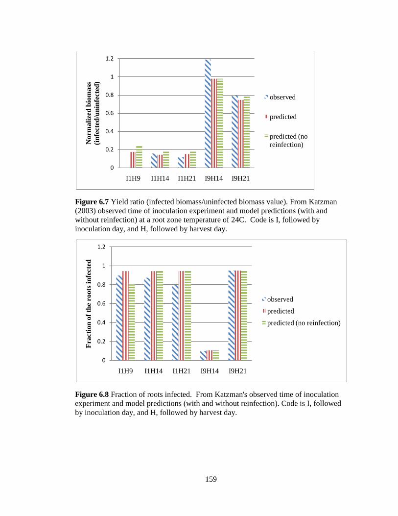
159
Figure 6.7 Yield ratio (infected biomass/uninfected biomass value). From Katzman
(2003) observed time of inoculation experiment and model predictions (with and
without reinfection) at a root zone temperature of 24C. Code is I, followed by
inoculation day, and H, followed by harvest day.
Figure 6.8 Fraction of roots infected. From Katzman's observed time of inoculation
experiment and model predictions (with and without reinfection). Code is I, followed
by inoculation day, and H, followed by harvest day.
0
0.2
0.4
0.6
0.8
1
1.2
I1H9 I1H14 I1H21 I9H14 I9H21
No
rma
lize
d b
iom
ass
(in
fect
ed/u
nin
fect
ed)
observed
predicted
predicted (no
reinfection)
0
0.2
0.4
0.6
0.8
1
1.2
I1H9 I1H14 I1H21 I9H14 I9H21
Fra
ctio
n o
f th
e ro
ots
in
fect
ed
observed
predicted
predicted (no reinfection)
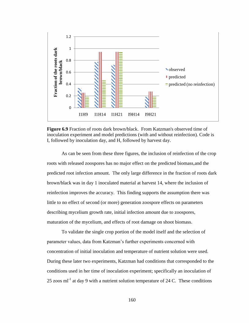
160
Figure 6.9 Fraction of roots dark brown/black. From Katzman's observed time of
inoculation experiment and model predictions (with and without reinfection). Code is
I, followed by inoculation day, and H, followed by harvest day.
As can be seen from these three figures, the inclusion of reinfection of the crop
roots with released zoospores has no major effect on the predicted biomass,and the
predicted root infection amount. The only large difference in the fraction of roots dark
brown/black was in day 1 inoculated material at harvest 14, where the inclusion of
reinfection improves the accuracy. This finding supports the assumption there was
little to no effect of second (or more) generation zoospore effects on parameters
describing mycelium growth rate, initial infection amount due to zoospores,
maturation of the mycelium, and effects of root damage on shoot biomass.
To validate the single crop portion of the model itself and the selection of
parameter values, data from Katzman‟s further experiments concerned with
concentration of initial inoculation and temperature of nutrient solution were used.
During these later two experiments, Katzman had conditions that corresponded to the
conditions used in her time of inoculation experiment; specifically an inoculation of
25 zoos ml-1
at day 9 with a nutrient solution temperature of 24 C. These conditions
0
0.2
0.4
0.6
0.8
1
1.2
I1H9 I1H14 I1H21 I9H14 I9H21
Fra
ctio
n o
f th
e ro
ots
da
rk
bro
wn
/bla
ck
observed
predicted
predicted (no reinfection)
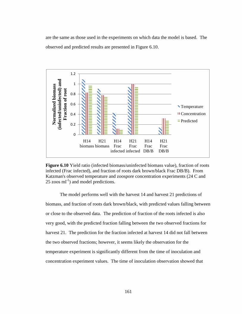
161
are the same as those used in the experiments on which data the model is based. The
observed and predicted results are presented in Figure 6.10.
Figure 6.10 Yield ratio (infected biomass/uninfected biomass value), fraction of roots
infected (Frac infected), and fraction of roots dark brown/black Frac DB/B). From
Katzman's observed temperature and zoospore concentration experiments (24 C and
25 zoos ml-1
) and model predictions.
The model performs well with the harvest 14 and harvest 21 predictions of
biomass, and fraction of roots dark brown/black, with predicted values falling between
or close to the observed data. The prediction of fraction of the roots infected is also
very good, with the predicted fraction falling between the two observed fractions for
harvest 21. The prediction for the fraction infected at harvest 14 did not fall between
the two observed fractions; however, it seems likely the observation for the
temperature experiment is significantly different from the time of inoculation and
concentration experiment values. The time of inoculation observation showed that
0
0.2
0.4
0.6
0.8
1
1.2
H14
biomass
H21
biomass
H14
Frac
infected
H21
Frac
infected
H14
Frac
DB/B
H21
Frac
DB/B
Norm
ali
zed
bio
mass
(in
fect
ed/u
nin
fect
ed)
an
d
Fra
ctio
n o
f ro
ot
Temperature
Concentration
Predicted

162
0.10 of the roots were infected at harvest 14, which agrees very closely with the
concentration observation of 0.117 and the predicted value of 0.106.
To validate the portion of the model concerned with the effects of nutrient
solution temperature on the growth of mycelium and effect on crop biomass, the
model was run with the same conditions as Katzman‟s nutrient solution temperature
experiment. The results are presented in Figure 6.11, Figure 6.12 and Figure 6.13.
Predicted values both with and without reinfection were calculated to illustrate the
effect of secondary infection, particularly at higher temperatures.
Figure 6.11 Yield ratio (infected biomass/uninfected biomass value) at harvest. From
Katzman's nutrient solution temperature experiment and model predictions. Code is
temperature followed by harvest day.
0
0.2
0.4
0.6
0.8
1
1.2
18C
H14
24C
H14
30C
H14
18C
H21
24C
H21
30C
H21
Norm
ali
zed
bio
mass
(in
fect
ed/u
nin
fect
ed)
observed
predicted
predicted (no reinfection)

163
Figure 6.12 Fraction of root infected. From Katzman's nutrient solution temperature
experiment, and model predictions. Code is temperature followed by harvest day.
Figure 6.13 Fraction of root dark brown/black. From Katzman's nutrient solution
temperature experiment, and model predictions. Code is temperature followed by
harvest day.
0
0.2
0.4
0.6
0.8
1
1.2
18C
H14
24C
H14
30C
H14
18C
H21
24C
H21
30C
H21
Fra
ctio
n o
f ro
ot
infe
cted
observed
predicted
predicted (no reinfection)
0
0.2
0.4
0.6
0.8
1
1.2
18C
H14
24C
H14
30C
H14
18C
H21
24C
H21
30C
H21
Fra
ctio
n o
f ro
ot
dark
bro
wn
/bla
ck
observed
predicted
predicted (no
reinfection)

164
The model reasonably predicts harvest biomasses (Figure 6.11) for the two
lower temperature conditions, 18 and 24C, underestimating them by 1 to 2% at harvest
14, and 4 and 15% at harvest day 21 (assuming the observed harvest biomass fractions
at 24C Harvest 14 and 18C harvest 21 are 1 and not 1.09 and 1.11 respectively).
However, for the 30C harvest day 14 condition it predicted a harvest biomass fraction
of 0.975, as compared to an observed biomass fraction of 0.65. The 30C harvest 21
condition prediction was even worse with a predicted fraction of 0.701 versus an
observed fraction of 0.3. There was very little difference between the predictions with
and without reinfection.
The model predicted well the fraction of the roots infected (Figure 6.12) at
harvest 21, for all three temperature conditions. However, it overestimated the values
at harvest 14 for both the 24 and 30C condition (though as has been described
previously the observed value is quite different and so the prediction is actually closer
to the other observed values. The 30C fraction was considerably underestimated
(33%).
The model also predicted quite well the fraction of the roots dark brown/black
(Figure 6.13) for the 18 and 24C temperature conditions at both harvest 14 and 21.
The model also significantly underestimated the values for the harvest day 14, 30C
condition, however the day 21 condition only differed by 4% (though this level is
close to the upper limit the model permits).
In these results there was little difference between the predictions using
reinfection and predictions without. This lack of difference is because the dose of 25
zoospores ml-1
was large enough that it reduced the possibility for further zoospores to
cause any more damage; second generation zoospores could not make things much
worse.
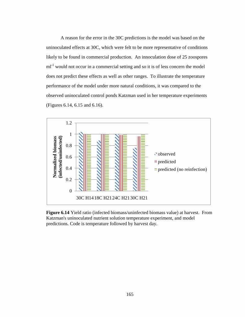
165
A reason for the error in the 30C predictions is the model was based on the
uninoculated effects at 30C, which were felt to be more representative of conditions
likely to be found in commercial production. An innoculation dose of 25 zoospores
ml-1
would not occur in a commercial setting and so it is of less concern the model
does not predict these effects as well as other ranges. To illustrate the temperature
performance of the model under more natural conditions, it was compared to the
observed uninoculated control ponds Katzman used in her temperature experiments
(Figures 6.14, 6.15 and 6.16).
Figure 6.14 Yield ratio (infected biomass/uninfected biomass value) at harvest. From
Katzman's uninoculated nutrient solution temperature experiment, and model
predictions. Code is temperature followed by harvest day.
0
0.2
0.4
0.6
0.8
1
1.2
30C H1418C H2124C H2130C H21
Norm
ali
zed
bio
mass
(in
fect
ed/u
nin
fect
ed)
observed
predicted
predicted (no reinfection)
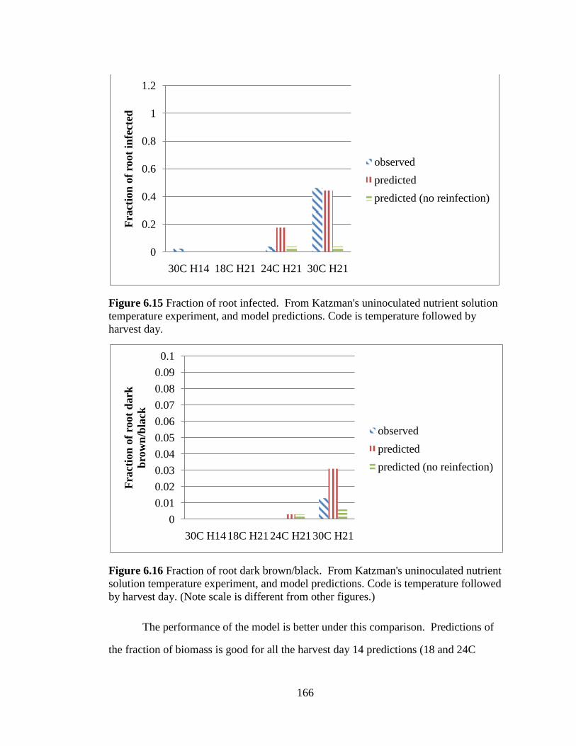
166
Figure 6.15 Fraction of root infected. From Katzman's uninoculated nutrient solution
temperature experiment, and model predictions. Code is temperature followed by
harvest day.
Figure 6.16 Fraction of root dark brown/black. From Katzman's uninoculated nutrient
solution temperature experiment, and model predictions. Code is temperature followed
by harvest day. (Note scale is different from other figures.)
The performance of the model is better under this comparison. Predictions of
the fraction of biomass is good for all the harvest day 14 predictions (18 and 24C
0
0.2
0.4
0.6
0.8
1
1.2
30C H14 18C H21 24C H21 30C H21
Fra
ctio
n o
f ro
ot
infe
cted
observed
predicted
predicted (no reinfection)
0
0.01
0.02
0.03
0.04
0.05
0.06
0.07
0.08
0.09
0.1
30C H14 18C H21 24C H21 30C H21
Fra
ctio
n o
f ro
ot
dark
bro
wn
/bla
ck
observed
predicted
predicted (no reinfection)

167
conditions were not shown as there was no Pythium damage apparent at that point).
Harvest day 21 predictions are also good for the 18 and 24 C temperatures, however,
the biomass fraction for the 30 C condition was overestimated by 20%.
The fraction of roots infected was a good fit, although this is also due to the
fact some of the parameters used to form the model were taken from these
observations. It is clear from Figure 6.15, the effects of reinfection are very important
in high temperature conditions.
The fraction of roots that are dark brown/black are also predicted very well
under all conditions, though this is partially due to the fact the values are low
compared to other inoculated infections (note scale of Figure 6.16 is adjusted to assist
in making comparisons).
To validate the portion of the model concerned with the effects of inoculum
concentration effects on the growth of mycelium and effect on crop biomass, the
model was run with the same conditions as Katzman‟s inoculation dosage experiment.
The results are presented in Figure 6.17, Figure 6.18 and Figure 6.19.
Figure 6.17 Yield ratio (infected biomass/uninfected biomass value) at harvest. From
Katzman's inoculation concentration experiment, and model predictions. Code is
zoospore concentration (zoos ml-1
) followed by harvest day.
0
0.2
0.4
0.6
0.8
1
1.2
0.025
H14
0.25
H14
2.5
H14
25
H14
250
H14
0.025
H21
0.25
H21
2.5
H21
25
H21
250
H21
Norm
ali
zed
bio
mass
(in
fect
ed/u
nin
fect
ed)
observed
predicted

168
Figure 6.18 Fraction of roots infected. From Katzman's inoculation concentration
experiment, and model predictions. . Code is zoospore concentration (zoos ml-1
)
followed by harvest day.
Figure 6.19 Fraction of root dark brown/black. From Katzman's inoculation
concentration experiment, and model predictions. . Code is zoospore concentration
(zoos ml-1
) followed by harvest day.
The model overpredicts harvest biomass at all concentrations of starting
inoculum for harvest 14 (with the exception of 0.25 zoos ml-1
), whereas, it
underestimates harvest biomasses for harvest day 21 with the exception of the highest
concentration, 250 zoos ml-1
where the estimate is 0.094 higher. Furthermore, the
0
0.2
0.4
0.6
0.8
1
1.2
0.025
H14
0.25
H14
2.5
H14
25
H14
250
H14
0.025
H21
0.25
H21
2.5
H21
25
H21
250
H21
Fra
ctio
n o
f ro
ots
in
fect
ed
observed
predicted
0
0.2
0.4
0.6
0.8
1
1.2
0.025
H14
0.25
H14
2.5
H14
25
H14
250
H14
0.025
H21
0.25
H21
2.5
H21
25
H21
250
H21
Fra
ctio
n o
f ro
ots
dark
bro
wn
/bla
ck
observed
predicted

169
model does not demonstrate as much of an effect of concentration, as is apparent in
the observed data. The observed biomass data of harvest 14 is difficult to use as any
differences (but for the highest concentration) were within the experimental error.
For the harvest 21 observed data, there is a difference of 0.25 between the lowest and
highest concentrations of inoculation, whereas, the model only predicts a difference of
0.104.
The model is better at predicting the fraction of root infected. It slightly over
and underpredicts the fraction of roots that are infected for the day 14 harvest. For the
day 21 harvest it is close in all concentrations but for the lowest where it overestimates
the fraction of roots infected by 0.288. As with biomass, the differential between the
highest and lowest concentrations are smaller in the predicted than the observed data.
The observed data had a differential of 0.167 as compared to a prediction of 0.075 in
the harvest day 14 conditions. In harvest day 21 conditions, excluding the lowest
concentration, the observed differential was 0.08 (0.32 with the lowest concentration)
whereas, the model predicted no difference between the highest and lowest
concentrations, as the prediction was at the model limit of 0.95 infection.
For the fraction of the root that is dark/brown black, the model performed well
for the harvest day 14 data, where no material was observed to be dark/brown black in
any condition, and the model predicted the same (< 0.01). For harvest day 21
predictions, the model underpredicted the fraction (but for the 2.5 zoos ml-1
condition)
and increased from 0.144 at 0.025 zoos ml-1
to 0.317 for the 250 zoos ml-1
condition.
The observed fractions ranged from 0.153 to 0.388.
Validation of multi cohort Pythium disease model parameters
The multi-cohort performance of the disease model was validated with data
from the purposely inoculated conditions presented in chapter 3. Two sets are used;

170
high temperature inoculation, and temperature suppression inoculation. In the high
temperature inoculation, the system was run with a nutrient solution of 27.5C until a
stand of 5 cohorts (aged 1, 4, 7, 10 and 13 days from floatation) was established. At
this time, an inoculum dosage of 100 zoos ml-1
was added. The plants were harvested
when each cohort was 14 days old, and new cohorts were added every three days. The
temperature suppression examination started out the same, however, 24 hours after
inoculation with 100 zoos ml-1
, the temperature of the nutrient solution was lowered
from 27.5C to 20C. The harvesting and addition of new cohorts followed the same
pattern as the high temperature inoculation set.
To validate the multi cohort portion of the Pythium disease model, the
conditions used in these two studies were input into the disease model, which was
extended to handle multiple cohorts in a common pond of nutrient solution. The
observed experimental results were normalized by dividing the infected harvest
biomasses by the corresponding uninfected control biomasses and plotted with the
predicted yield ratio harvest biomasses in Figure 6.20 and Figure 6.21.
Figure 6.20 Yield ratio (infected biomass/uninfected biomass value) for a warm
temperature nutrient solution (27.5C) inoculated with 100 zoos ml-1
for one sequence
of harvests. (A new cohort was added every 3 days, harvested after 14 days for a total
experimental time of 41 days.)
0
0.2
0.4
0.6
0.8
1
1.2
1.4
0 2 4 6 8 10 12
No
rma
lize
d h
arv
est
bio
mass
(in
fect
ed/u
nin
fect
ed)
Harvest number
observed
predicted

171
In Figure 6.20, the predicted harvest biomasses follow the same trend as the
observed data, showing a steep decline followed by a stable harvest biomass amount
as the disease stabilizes in the crop. Differences between observed and modeled data
are the model predicts a less severe drop off, and the level of disease settled out to
about one third of that observed, but close in absolute values.
Figure 6.21 Yield ratio of biomasses (infected/uninfected) for an initially warm
temperature nutrient solution (27.5C) inoculated with 100 zoos ml-1, switched to a
cold (20C) temperature nutrient solution, 24 hours after inoculation.
The performance of the model to predict the response of the system to a switch
to a cold nutrient solution temperature (Figure 6.21) appears to be very good. Though
the model predicts a higher level of damage in the fifth harvest material, it correctly
predicts the harvest biomasses of material not directly exposed to the initial
inoculation dose would be close to the uninoculated control. However, the model still
predicts some level of damage in the crop as the harvest six biomasses do not
immediately return to an uninfected state as would be represented by a normalized
value of one. As in the high temperature inoculation simulation shown in Figure 6.20,
the differences of Figure 6.21 may also be explained by temperature. The reduction at
harvest 5 is the youngest material present in the system when the inoculation was
0
0.2
0.4
0.6
0.8
1
1.2
0 2 4 6 8 10Norm
ali
zed
harv
est
bio
mass
(in
fect
ed/u
nin
fect
ed)
Harvest Number
observed
predicted

172
applied. It was exposed to high temperatures in the presence of a high inoculation
dosage and, as in the situation previously described, the model predicted more damage
than was observed. The fact the harvests did not return to a completely uninfected
state following the dropping of the temperature could be due to the fact the cool
temperature applied was 20C (again, not a temperature Katzman used). From the
Katzman data it is impossible to say what the safe cut-off temperature would be for a
14 day crop cycle. A temperature of 18 appears to be safe, but as observed in the
multi-cohort work 20C, also appears adequate.
A further check on the functionality of the model is how the length of the crop
cycle and temperature of the nutrient solution, affect the number of harvests before the
harvested material is too badly damaged by Pythium to sell (Table 6.8). This measure
is different from merely observing the drop in normalized biomass as was done in
figures 6.20 and 6.21. Though biomass may not be largely affected, if the roots are 10
to 15% infected, there is some wilting present in the crop, which in turn makes the
material unsaleable. To determine the values presented in Table 6.9, the model was
run with different crop lengths, and nutrient solution temperatures. Harvests were
counted as successful, if they had less than 15% of their roots infected.
Table 6.9 Number of harvests (based on a 3 day harvest schedule in a continuous
production pond) before crop material is too badly damaged by Pythium to market, as
a function of nutrient solution temperature. Grown at 18 to 32 C for 14 to 22 days.
Temperature C
18 20 22 24 26 27.5 30 32
Crop
Length
(days)
14 >50 >50 >50 >50 >50 >50 >50 3
16 >50 >50 >50 >50 >50 >50 2 1
18 >50 >50 >50 >50 4 2 1 0
20 >50 >50 >50 >50 1 0 0 0
22 >50 >50 >50 0 0 0 0 0
173
The trend presented in Table 6.9 is as expected. As the length of time the crop spends
in the pond increases (increasing crop length), there is increased time for reproduction
and release of zoospores to newer cohorts of the crop. Increasing nutrient solution
temperature accelerates this process, and at higher temperatures the number of
successful harvests before collapse is reduced. Because of the form of the model, it
appears to be very sensitive to critical points, where below a specific temperature
infections do not develop, and only a degree or half a degree higher and major
problems result. This sensitivity is also apparent in the results of table 6.8 where
several combinations of temperature and crop length result in no crop losses (at least
in the observed period of 50 harvests). This lack of outbreaks does not seem as
plausible as other results of the model. However, the model is assuming growing and
disease conditions that are unlikely to exist in real world production. Constant
temperatures, and constant disease and crop growth factors are an assumption of the
model that may not be satisfied in the real world. In addition, it is assumed the crop is
never under any stresses, which could make it more susceptible to infection. Though
the results presented in Table 6.9 may not exactly correspond to what one would
expect, the trends presented do, and as such the model may be useful for making
comparisons of various production techniques.
6.4.2 Sensitivity analysis of Pythium disease model parameters
By plotting the parameters of the model in tornado style, it is possible to see
the effect of each parameter on the final outcome. To generate the tornado plots, the
model was run twice for each parameter; once with the value of the parameter
increased 10% and once with the value decreased 10%. The output of the model was
recorded for each run, and then summarized in tornado plots. A complicating factor is
the model is developed to function from a number of different starting points and

174
different conditions. Because certain variables become more important under different
conditions it was necessary to create several tornado plots.
The parameters examined are:
1. βconc, Concentration effect slope
2. αconc, Concentration effect intercept
3. εmycelium, Reference amount of mycelium @ 25 zoos ml-1
4. M0, Starting Mass of mycelium
5. βgrow, Mycelial growth rate slope
6. αgrow, Mycelial growth rate intercept
7. Amature, Maturation age of mycelium
8. ηphoto, Coefficient of Photosynthetic Rate reduction
9. βtemp, Temperature effect slope
10. αtemp, Temperature effect intercept
11. Arelease, Zoospore release age
12. Nzoos, Zoospore release amount
To examine the effect of each variable under the conditions used to develop the
model in the first place, 15 tornado plots were necessary. These plots represent the
output of the model with two inoculation days (day 1 and day 9), three harvest days
(days 9, 14 and 21) and for the three output values of the model, fraction of uninfected
biomass, fraction of the roots uninfected, and fraction of the roots dark brown/black.
The day 9 inoculation and day 9 harvest combination were dropped as no significant
effects of Pythium were observed. The results of this examination are shown in Figure
6.22 to Figure 6.36.

175
Figure 6.22 Sensitivity of the fraction of uninfected biomass to model parameters with
inoculation on day 1 and harvest on day 9 with a nutrient solution of 24 C.
Figure 6.23 Sensitivity of the fraction of uninfected roots to model parameters with
inoculation on day 1 and harvest on day 9 with a nutrient solution of 24 C.
0 0.1 0.2 0.3 0.4 0.5
M0Nzoos
Amatureβgrow
Arelease
βconcαgrowαtempαconc
εmyceliumηphotoβtemp
Fraction of uninfected Biomass
0.94 0.942 0.944 0.946 0.948 0.95
M0Nzoos
Areleaseβconcβgrow
Amatureβtempαtempαconcαgrow
εmyceliumηphoto
Fraction of uninfected roots
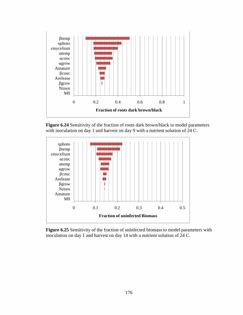
176
Figure 6.24 Sensitivity of the fraction of roots dark brown/black to model parameters
with inoculation on day 1 and harvest on day 9 with a nutrient solution of 24 C.
Figure 6.25 Sensitivity of the fraction of uninfected biomass to model parameters with
inoculation on day 1 and harvest on day 14 with a nutrient solution of 24 C.
0 0.2 0.4 0.6 0.8 1
M0Nzoosβgrow
Areleaseβconc
Amatureαgrowαconcαtemp
εmyceliumηphotoβtemp
Fraction of roots dark brown/black
0 0.1 0.2 0.3 0.4 0.5
M0Amature
Nzoosβgrow
Arelease
βconcαgrowαtempαconc
εmyceliumβtemp
ηphoto
Fraction of uninfected Biomass
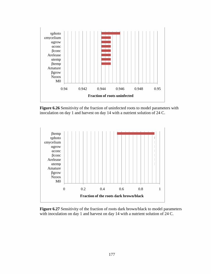
177
Figure 6.26 Sensitivity of the fraction of uninfected roots to model parameters with
inoculation on day 1 and harvest on day 14 with a nutrient solution of 24 C.
Figure 6.27 Sensitivity of the fraction of roots dark brown/black to model parameters
with inoculation on day 1 and harvest on day 14 with a nutrient solution of 24 C.
0.94 0.942 0.944 0.946 0.948 0.95
M0Nzoosβgrow
Amatureβtemp
αtempArelease
βconcαconcαgrow
εmyceliumηphoto
Fraction of roots uninfected
0 0.2 0.4 0.6 0.8 1
M0Nzoosβgrow
Amatureαtemp
Areleaseβconcαconcαgrow
εmycelium
ηphotoβtemp
Fraction of the roots dark brown/black

178
Figure 6.28 Sensitivity of the fraction of uninfected biomass to model parameters with
inoculation on day 1 and harvest on day 21 with a nutrient solution of 24 C.
Figure 6.29 Sensitivity of the fraction of uninfected roots to model parameters with
inoculation on day 1 and harvest on day 21 with a nutrient solution of 24 C.
0 0.1 0.2 0.3 0.4 0.5
M0Amature
Nzoosβgrow
Arelease
βconcαtempαgrowαconc
εmyceliumβtemp
ηphoto
Fraction of uninfected Biomass
0.94 0.942 0.944 0.946 0.948 0.95
M0Nzoos
Areleaseβconcβgrow
Amatureηphotoβtempαtempαconcαgrow
εmycelium
Fraction of the roots infected

179
Figure 6.30 Sensitivity of the fraction of roots dark brown/black to model parameters
with inoculation on day 1 and harvest on day 21 with a nutrient solution of 24 C.
Figure 6.31 Sensitivity of the fraction of uninfected biomass to model parameters with
inoculation on day 9 and harvest on day 14 with a nutrient solution of 24 C.
0.94 0.942 0.944 0.946 0.948 0.95
M0Nzoos
Areleaseβconcβgrow
Amatureηphotoβtempαtempαconcαgrow
εmycelium
Fraction of the roots dark brown/black
0.95 0.96 0.97 0.98 0.99 1
M0Nzoos
Areleaseβgrowαgrow
Amatureβconcαtempαconc
εmyceliumηphotoβtemp
Fraction of uninfected Biomass

180
Figure 6.32 Sensitivity of the fraction of uninfected roots to model parameters with
inoculation on day 9 and harvest on day 14 with a nutrient solution of 24 C.
Figure 6.33 Sensitivity of the fraction of roots dark brown/black to model parameters
with inoculation on day 9 and harvest on day 14 with a nutrient solution of 24 C.
0 0.05 0.1 0.15 0.2 0.25
M0Nzoosβgrowαgrow
Amature
ηphotoArelease
βconcαconcαtemp
εmyceliumβtemp
Fraction of roots infected
0 0.005 0.01 0.015 0.02 0.025
M0Nzoos
Areleaseβconcαconc
βgrowαgrow
εmyceliumηphotoαtemp
Amatureβtemp
Fraction of the roots dark brown/black
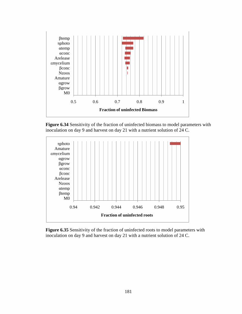
181
Figure 6.34 Sensitivity of the fraction of uninfected biomass to model parameters with
inoculation on day 9 and harvest on day 21 with a nutrient solution of 24 C.
Figure 6.35 Sensitivity of the fraction of uninfected roots to model parameters with
inoculation on day 9 and harvest on day 21 with a nutrient solution of 24 C.
0.5 0.6 0.7 0.8 0.9 1
M0βgrowαgrow
AmatureNzoos
βconcεmycelium
Areleaseαconcαtemp
ηphotoβtemp
Fraction of uninfected Biomass
0.94 0.942 0.944 0.946 0.948 0.95
M0βtempαtempNzoos
Arelease
βconcαconcβgrowαgrow
εmyceliumAmature
ηphoto
Fraction of uninfected roots

182
Figure 6.36 Sensitivity of the fraction of roots dark brown/black to model parameters
with inoculation on day 9 and harvest on day 21 with a nutrient solution of 24 C.
It is not surprising the variable to which the model is the most sensitive is the
slope of the temperature effects, βtemp. In the model, it is assumed the temperature
affects not only the growth rate of the mycelia, but the developmental rate as well.
The intercept of the temperature effects, αtemp, is also important, though it is not as
powerful as the slope, βtemp.
Another expected effect is the sensitivity of the model to the coefficient of
Photosynthetic Rate reduction, ηphoto, particularly examining the fraction of the
uninfected biomass. ηphoto relates the amount of infection in the roots to the reduction
in photosynthate production, which directly affects the accumulation of plant biomass.
The initial amount of mycelium, M0, appears to have no effect on the model at
all. However, this lack of effect is because these plots examined conditions in which
the crop was inoculated with a large single dose of zoospores, causing massive
damage and overwhelming any effect the natural inoculum present might have had.
To examine the sensitivity of the model to parameters under conditions more
likely to be found in a commercial setting, the sensitivity analysis was run with no
0 0.2 0.4 0.6 0.8 1
M0βgrowαgrowNzoos
ηphoto
βconcεmycelium
αconcAreleaseAmature
αtempβtemp
Fraction of roots dark brown/black
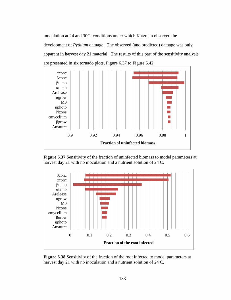
183
inoculation at 24 and 30C; conditions under which Katzman observed the
development of Pythium damage. The observed (and predicted) damage was only
apparent in harvest day 21 material. The results of this part of the sensitivity analysis
are presented in six tornado plots, Figure 6.37 to Figure 6.42.
Figure 6.37 Sensitivity of the fraction of uninfected biomass to model parameters at
harvest day 21 with no inoculation and a nutrient solution of 24 C.
Figure 6.38 Sensitivity of the fraction of the root infected to model parameters at
harvest day 21 with no inoculation and a nutrient solution of 24 C.
0.9 0.92 0.94 0.96 0.98 1
Amature
βgrow
εmycelium
Nzoos
ηphoto
M0
αgrow
Arelease
αtemp
βtemp
βconc
αconc
Fraction of uninfected biomass
0 0.1 0.2 0.3 0.4 0.5 0.6
Amatureηphotoβgrow
εmyceliumNzoos
M0αgrow
Areleaseαtempβtempαconcβconc
Fraction of the root infected

184
Figure 6.39 Sensitivity of the fraction of the root dark brown/black to model
parameters at harvest day 21 with no inoculation and a nutrient solution of 24 C.
Figure 6.40 Sensitivity of the fraction of uninfected biomass to model parameters at
harvest day 21 with no inoculation and a nutrient solution of 30 C.
0 0.002 0.004 0.006 0.008 0.01 0.012 0.014
M0Nzoos
Areleaseβgrowαgrow
εmyceliumηphoto
Amatureαtempαconcβconcβtemp
Fraction of the root dark brown/black
0.7 0.75 0.8 0.85 0.9 0.95 1
Amature
βgrow
εmycelium
ηphoto
Nzoos
M0
αgrow
αtemp
Arelease
βtemp
βconc
αconc
Fraction of uninfected Biomass

185
Figure 6.41 Sensitivity of the fraction of the root infected to model parameters at
harvest day 21 with no inoculation and a nutrient solution of 30 C.
Figure 6.42 Sensitivity of the fraction of the root dark brown/black to model
parameters at harvest day 21 with no inoculation and a nutrient solution of 30 C.
The parameter to which the model is most sensitive, when considering a
naturally developing infection (uninoculated), is the concentration effects on slope and
intercept. This variable defines how much damage free zoospores in solution do to the
roots. It becomes important under these conditions because at harvest day 21 under
0 0.2 0.4 0.6 0.8 1
Amatureηphotoβgrow
εmyceliumNzoos
M0αgrowαtemp
Areleaseβtempβconcαconc
Fraction of roots infected
0 0.2 0.4 0.6 0.8 1
ηphoto
βgrowεmycelium
NzoosM0
αgrowAreleaseAmature
αtempβtempαconcβconc
Fraction of roots dark brown/black

186
both temperatures Pythium has had enough time to complete its reproductive cycle and
release zoospores from the initial infection amount. At the higher 30C temperature,
this effect is even more apparent as the mycelium develops and grows faster as
temperature increases.
As in the case of the inoculated conditions temperature effect variables
continue to be important to the model. Speeding or slowing the rate of growth of the
mycelium and regulating the time of release of the zoospores results in variables that
are very important in a naturally developing infection.
The zoospore releasing age, Arelease, also plays a noticeable role under these
conditions. This variable controls when the mycelium has matured enough to release
zoospores, which furthers the infection. The number of zoospores released, nzoos,
plays less of a role.
6.5 DISCUSSION:
The first objective of this chapter was to develop a framework and parameters
for a model to predict the growth and spread of Pythium aphanidermatum in a
hydroponic baby spinach crop grown under controlled environment conditions. To
accomplish this goal, data from Katzman‟s study of Pythium (Katzman 2003) in
individual spinach crops grown under a variety of conditions was combined with
observations made during the NYSERDA spinach disease project (Albright et al.,
2007). Katzman‟s data formed the basis for the model, whereas, the NYSERDA data
was used to validate the developed model in multi-cohort production. The core of the
disease model is the hour by hour tracking of the growth and development of the
Pythium mycelia on the roots of each cohort of spinach. Through the examination of
Katzman‟s data it was possible to deduce a growth rate for the mycelium. The
remainder of the parameters of the model followed; using the estimated growth rate

187
and further data to expand the functionality of the model piece by piece, until it
encompassed the anticipated scope of its utility.
The second objective was to modify the SUCROS based baby spinach growth
model to take into account the damage done to the roots due to Pythium
aphanidermatum zoospores and mycelia on crop growth. SUCROS was chosen as a
model because it tracks growth of both the roots and shoots. The shoots are of
primary interest to a grower as that is the part of the crop harvested and sold. The
roots are of particular interest because they are the target of Pythium, and impact the
ability of a crop to transpire and grow. The disease model was developed so a
variable, the coefficient of photosynthetic rate reduction, linked the damage in the
roots to the reduction in the crop‟s ability to generate photosynthates, which are the
building blocks of the crop.
The final objective of the chapter was to validate the model by comparing
predicted crop growth and Pythium disease damage to experimentally collected data.
The model quite accurately predicts the growth of the crop, and the spread of Pythium
under the conditions from which it was developed in Katzman‟s experiments. It also
accurately predicts the development and spread of a Pythium infection in a multi-
cohort situation, where several differently aged cohorts of spinach are present within a
common nutrient solution, such as was studied in the NYSERDA disease project.
The model successfully captures the sensitivity of the spread of Pythium to the
temperature of the nutrient solution. In the sensitivity analyses the variables
controlling the response of the growth rate, and the maturation of the mycelium to
temperature, exerted the most influence over the outcomes of the model under the
conditions examined. This result follows the major finding of Katzman, and the
NYSERDA disease project.

188
A major assumption of the model was that damage due to second generation
zoospores was not a significant part of the observed damage in the 18C and 24C
temperature conditions. This assumption simplified the development of the mycelium
growth rate, and the temperature response curve. This assumption was shown to be
valid when the output of the model both with and without reinfection was compared to
the observations made in Katzman‟s experiments.
A shoot quality index was included in the model because Katzman showed
small amounts of root damage (10 to 15% infected root) lead to some wilting in the
crop. Even a small amount of wilting is unacceptable to a grower as it can lead to
rapid decay following harvest. Using strictly biomass as a metric for crop failure
would miss this important aspect as biomass does not decrease as soon as Pythium
appears. In the calculation of the number of harvests until crop failure as a function of
temperature and crop duration, it was apparent by examining biomass data only, one
would miss the wilting aspect of crop production. Inclusion of crop quality index also
allows better modeling of grower response to disease. Material that is wilting and
showing signs of infection would be removed as soon as or shortly after it is apparent,
as there is no commercial value in continuing that particular cohort.
A primary discrepancy in the model is the number of harvests until failure
seems too forgiving of high temperatures and longer crop cycles. However, the
number of harvests might be deceiving as it does not represent successive harvests,
rather harvests of separate cohorts spaced three days apart. The model is based on
data from Katzman and her growing conditions which were primarily concerned with
single crop production, and the extension to multi-cohort systems goes beyond the
scope of her work. What is more problematic is the sensitivity of the model to the
temperature and crop length. At one temperature, production collapses within four
harvests, but only two degrees cooler in the nutrient solution and production appears

189
safe. One would expect rather than be safe, the number of harvests until collapse
would merely increase, perhaps by a large amount, but failure would be inevitable.
However, it is possible this result is more a function of the conditions the crop is
exposed to rather than a serious flaw in the model. The model assumes the rather
unlikely condition that the parameter values of the crop growth and the Pythium
disease model are constant in time, and environmental conditions remain constant as
well. The model also neglects the effects any temporary stresses might have on the
susceptibility of the crop to Pythium. In many of the combinations of temperature and
crop duration where the model predicts no problem, it is likely a slight imbalance or
temporary change in conditions could push the crop into runaway failure. Monte-
Carlo simulation of the model, where the parameters of the model are randomly
varied, would present a more realistic summation of the performance of the model by
having probability distributions in place of the all or nothing results generated by the
constant values of this model.
A potential problem with the model is it was primarily developed from data
where the experimental ponds were inoculated with artificially high levels of
zoospores, unlikely to be encountered in a natural setting except in the cases of
extremely progressed infections. The purpose of the model, however, is to predict
how infections develop in commercial settings where large scale inoculations will not
occur. Thus it was necessary to extrapolate the performance of the model in a multi-
cohort naturally occurring infection from the unintentional damage observed in
Katzman‟s control crops. However, even if the absolute timing of an infection due to
natural inoculation is not very accurate, the model provides a means of comparing
production strategies; not a definitive prediction of when an outbreak will occur.
The model is also not directly concerned with the accuracy of the prediction of
the final harvest weight of highly damaged crops. Though it may reasonably predict
190
such values, in a commercial setting such knowledge is unnecessary. If the crop is
unsaleable, the absolute biomass of the unsaleable crop is unimportant other than from
a waste management perspective.
Another consideration is the data on which the model is based was from a
highly regulated and frequently cleaned experimental setup. Such conditions are
unlikely to be found or maintained in a commercial setting, and as such the model is
most likely underestimating the rapidity with which a Pythium infection would
develop in an uninoculated commercial setting.
A major assumption of the model is zoospores do not carry over from hour to
hour. This model would predict that removing a crop and waiting an hour before
putting new material in, would break the disease cycle, however, in reality this is
certainly not the case. As such caution must be taken in using the model in situations
for which it was not developed.
A simplification was the model only considered light integrals have been done
in previous spinach work. Extending the use of the model to conditions outside of this
range will require the assumption that slowed (or increased) crop growth will not
affect the spread of Pythium beyond that which the model already accounts. The
model was developed using data from harvests conducted 21 days from seeding,
however, the light on the crop over the 21 days remained constant.
The temperature effects of the model were derived from only three points.
Though they span the range of temperatures usually encountered in greenhouses, care
should be taken not to extrapolate too far beyond this range. Further data collected at
additional temperatures would better characterize the temperature response.
Another major assumption of the model is the disease organism is Pythium
aphanidermatum. This is the organism identified by Katzman as present in the
Cornell greenhouses. However, Bates and Stanghellini (1984) found in Arizona the

191
disease organism of interest changed as the temperature of the nutrient solution shifted
with the season. Pythium dissotocum was found to become prevalent in the ponds of
the growing system when the temperature of the nutrient solution was below 23C.
However, a complicating factor is that lettuce was grown in the same ponds as the
spinach. Though seemingly unaffected by the presence of Pythium dissotocum, the
lettuce could have served as a reservoir of zoospores, accelerating the development of
the disease in the spinach crop. In addition, their production did not focus on a
babyleaf crop, where a shortened crop duration could have potentially overcome
dissotocum. Though dissotocum might function at temperatures below that of
aphanidermatum, there is the possibility that its rate of growth might be such it too
can be overcome by shortened crop cycles and perhaps even further temperature
reductions of the nutrient solution. Before the model is extended to encompass
Pythium dissotocum, further experiments with this organism must be carried out.

192
CHAPTER 7: SIMULATION OF SELECT PRODUCTION STRATEGIES
7.1 INTRODUCTION:
Though Pythium aphanidermatum is a major obstacle to commercial
hydroponic spinach production, it is not an insurmountable barrier. Commercial
hydroponic spinach production is practiced in Japan; however, their technique, namely
single use of the nutrient solution followed by extensive cleanout between crops, is
very expensive, both in terms of financial and environmental cost. To investigate
alternate means of production, NYSERDA (New York State Energy Research and
Development Authority) funded a project to examine both existing and new water
treatment technologies to remove Pythium from nutrient solutions and to evaluate
these treatment systems in both pond and aeroponic production (Albright et al. 2007).
Chapters two and three of this dissertation describe our work on this issue. The
primary findings of the NYSERDA Pythium project were there are many effective
means of killing and/or removing Pythium zoospores from the nutrient solution A
better alternative, however, was to take advantage of crop cultural practices to prevent
infection from propagating.
One of the findings of Katzman in her dissertation entitled, “Influence of Plant
age, Inoculum Dosage, and Nutrient Solution Temperature on the Development of
Pythium aphanidermatum in Hydroponic Spinach Production Systems” (2003) was
the Pythium disease reproductive cycle is highly temperature dependant. Similar
results were observed in the NYSERDA Spinach disease project where it was found
that by reducing the nutrient solution temperature, the reproductive time of Pythium
was increased. If the crop cycle is shorter than the time it takes for Pythium zoospores
to reach maturity and generate new zoospores, the infection would die out as infected
roots are removed at harvest without having a chance to release zoospores to further
the infection.

193
Using these findings, production strategies for commercial production of
hydroponic spinach have been developed. Various combinations of nutrient solution
cooling, two pond system, batch production and nutrient solution sterilization, result in
growing techniques with quite different risks of crop losses due to Pythium outbreaks
that vary under different climate conditions. However, the cost of implementing these
different strategies in terms of capital, labor and energy, are also quite different and
the decision of which system a grower should select is a combination of the estimated
risk of loss for their particular conditions and the cost of their chosen growing
technique.
Before investing in a large scale commercial production system, an
examination of the expected risk of loss due to Pythium is needed. Pilot scale testing
of production systems is one option, however, there are drawbacks associated with this
approach. Results of a pilot scale test would not necessarily translate to other
locations or regions where differences in climate could affect both the disease cycle
and/or the growth of the crop itself. Even though controlled environment systems
seek to manage environmental conditions within set targets, the cost of doing so may
be prohibitive. Pilot scale testing also has the drawback that conditions vary from year
to year, and extreme events could strain a system and natural variability in the climate
and disease parameters, may not be encountered. In addition, all the combinations of
alternative production methods would be difficult to fully test individually on a
meaningful scale and would be complicated by disease processes that are likely
seasonal, requiring year round studies.
An alternative, or at least a prelude to pilot scale testing, is to model the
environment-greenhouse-plant-disease relationship and use a stochastic simulation to
determine expected outcomes of different production strategies. The individual
variability of the parameters within this complex system can be estimated and
194
ultimately combined in a Monte-Carlo style simulation to provide an estimate of the
expected frequency of Pythium outbreaks.
To simulate the greenhouse response to environmental conditions, a stepwise
steady state model was developed (described in chapter four). This model takes
environmental inputs of solar radiation, outdoor temperature, and outdoor humidity
and, combined with typical greenhouse operational control strategies (light and
temperature), predicts the indoor PAR levels and air and pond temperatures.
Simulation of spinach growth is achieved by using the output of the greenhouse
simulation model as input to a modified SUCROS growth model adjusted for hourly
growth of spinach under both natural and supplemental lighting (described in chapter
five). Working in concert with the growth model is a Pythium disease model that
simulates the growth and spread of a Pythium infection in hydroponic pond production
and its effect on the growth of the spinach crop (described in chapter six). This
combined greenhouse-spinach-Pythium model system is used to explore the effects of
different production strategies and growing conditions on crop and Pythium disease
growth in this chapter.
Objectives:
1. simulate the production of hydroponic spinach in the presence of Pythium
aphanidermatum, under different production strategies,
2. develop quantitative measures of comparing the risk of Pythium damage
between the different production strategies,
3. present the results of the quantitative measures of the various production
strategies to assist in the selection of which strategies to investigate further at
pilot scale.
195
7.2 LITERATURE REVIEW:
7.2.1 Previous attempts to grow spinach hydroponically
One of the first attempts to grow commercial spinach hydroponically in the
United States was in Arizona, where both spinach and lettuce crops were grown in the
same ponds (Bates and Stanghellini, 1984). Production was carried out year round
with 2 week old seedlings (both spinach and lettuce) transplanted into floatation
boards and harvested 4 to 6 weeks later. The project commenced in September 1981
and by October 1981 extensive root damage, wilting and even death was apparent in
the spinach seedlings after they had spent 1 week in the system. Subsequent
investigation of the cause of the root damage identified Pythium aphanidermatum as
the causal agent of infection. At this time the temperature of the nutrient solution was
approximately 26C. Because Pythium aphanidermatum was known to be associated
with high temperatures the researchers felt as the season progressed into the winter
and nutrient solution temperatures dropped, the problem would go away. As the
season progressed and the nutrient solution temperature dropped to 22C, root rot and
plant death continued. However, another organism, Pythium dissotocum was isolated
from the roots of the infected crops. Though not as virulent as Pythium
aphanidermatum, Pythium dissotocum was able to infect and kill plants at the lower
temperatures and so the commercial spinach production part of the experiment was
abandoned.
Studies, however, were conducted to better understand the dynamics of the
infections. Throughout the course of a year 100 spinach seedlings were introduced
daily to a commercial lettuce pond. The percentage of plants showing stunting or
death was recorded every week. Two weeks after placement in the pond, the plants
were removed and 10 plants showing either death or infection had their roots analyzed
for the presence of Pythium aphanidermatum and Pythium dissotocum. The
196
temperature of the pond was recorded daily. Bates and Stanghellini found disease due
to Pythium occurred year round, however, the lowest disease incidence (< 25% of
plants stunted or dead) occurred in January and February when the nutrient solution
temperatures were below 20 C. For the remainder of the year when the nutrient
solution temperature was above 20 C, high disease incidence was apparent (>50% of
plants stunted or dead). Isolation of the causal agents from infected roots showed
Pythium dissotocum was the predominant or sole pathogen at temperatures below 23
C, whereas Pythium aphanidermatum was the predominant or sole pathogen above
23C. Both pathogens were seldom isolated from the same diseased root or plant. A
cycling of the pathogen make up with the seasonal temperature of the nutrient solution
was apparent. Subsequent investigations of metalaxyl (a fungicide primarily used for
soil borne pathogens) had some success in limiting root rot, but showed signs of
phytotoxicity at concentrations 10 µg a.i. ml-1
. Similarly treatments with chlorine,
zineb and captan were ineffective at controlling root rot and/or showed extreme
phytotoxicity, besides being not legal for use on crops for human consumption.
To date the only successful commercial spinach hydroponic production
systems have operated in Japan. It proved possible to grow spinach without
succumbing to root rot disease by using a batch production system where a single crop
is grown in a single pond, or NFT system and the nutrient solution discarded after
each crop and growing apparatus thoroughly cleaned. Of course, a major drawback
with this production system is the high cost. Nutrient solution is expensive, primarily
in terms of the cost of the clean water itself, and the cost of disposing of used solution.
In many locations, disposal of the nutrient solution is tightly regulated to prevent
contamination of ground and surface waters. Another disproportionately high expense
when compared to other production styles is the high labor associated with cleaning
between crops. Thoroughly cleaning the ponds, associated pumps and piping with
197
disinfectant, and rinsing everything, is a labor intensive process. The relatively short
crop cycle of spinach, coupled with the loss of growing area while cleaning is
conducted, lead to a very high cost of production. Perhaps only in Japan where a
premium price for quality and freshness can be realized, could such a system break
even. It is not clear whether the system is still operational, or if it was only run for
display purposes.
7.2.2 Cornell Experience with Hydroponic Spinach production
The investigation of hydroponic spinach production at Cornell started with the
use of a Nutrient Film technique (NFT) production system (Both et al 1996). Spinach
seedlings were started in rockwool slabs and transplanted to the NFT system after 8
days. 33 days after seeding a final harvest was conducted. The daily light integral
was varied to develop a growth curve for spinach. The results of this experiment were
confounded by Chlorine in the tap water (levels above 1 ppm were found to be
phytotoxic) and a root rot was identified as Fusarium. Treatment with fungicides and
potassium silicate were tried, but none proved successful in overcoming the root
disease problem.
The cause of the Fusarium infection was suspected to be contaminated seed
(Katzman 2003). Subsequent experiments in both NFT and pond systems exhibited
slightly different symptoms, which proved to be consistent with Pythium species.
Katzman (2003) investigated not only the possible sources of the infection, but also
examined the effects of plant age, inoculum dosage, and nutrient solution temperature
on the development of the disease. Concurrent with Katzman‟s research, a New York
State Energy Research and Development Authority (NYSERDA) grant (Albright et
al., 2005) allowed the examination of pond production of spinach. The NYSERDA
198
research was hampered by the fact pond solutions could not be reused and strict
hygiene had to be maintained at all times to prevent infection with Pythium.
Following the submission of the NYSERDA project final report, a second
NYSERDA grant was awarded to investigate both new and existing methods for
removing Pythium zoospores from the nutrient solution as well as how an alternate
growing system, aeroponics, would affect the development and spread of disease
(Albright et al., 2007). Aeroponics is a form of hydroponic production where the
nutrient solution is misted or sprayed onto the roots of the crop which dangle free in
the air. The theory behind selecting aeroponics for investigation with Pythium and
also examining nutrient solution treatment technologies is movement of zoospores
from infected plants could be stopped, or at least severely slowed. Pythium zoospores
move through the nutrient solution seeking out roots to infect. In aeroponics there is
no direct water connection between roots. Unused nutrient solution that drips off the
roots would be collected and treated to remove any zoospores present before being
resprayed onto the crop. Infected plants may suffer, but the infection should
theoretically not be able to progress from plant to plant. However, cultivating spinach
aeroponically proved to be very difficult. Nozzles were susceptible to clogging and
required frequent inspection to ensure an adequate flow of water to the roots. During
the day under high transpirational loads, wilting and death of plants could occur
rapidly if the spray was cut off. Other difficulties were due to the high plant densities
required for baby spinach production. High plant densities corresponded to dense root
mass, which made uniform distribution of the nutrient spray difficult. Root zone
temperature is difficult to control in aeroponics. The relatively small volume of
nutrient solution present in aeroponics systems is subject to relatively rapid changes of
air temperature. During the summer months, wilting and temperature stress were
apparent in the aeroponic system. Further investigation into aeroponics was

199
abandoned when it became apparent temperature control of the nutrient solution in
pond systems presented a viable means of production (as described in chapter three).
7.2.3 Cornell Experience with Hydroponic Pond production
The hydroponic system selected for the lettuce research module Cornell CEA
designed and operated was a pond system, on which 11 day old seedlings were
transplanted into floating Styrofoam boards at a spacing of 1.35E-2 m2
(21 square
inches) per plant. Following 11 days the crop is then transplanted to a final density of
2.71E-2 m2 (42 square inches) per plant, where it remains for 14 days until harvest.
There are many reasons a pond system was chosen over other systems such as NFT
(with which extensive lettuce work has been conducted at Cornell). One major benefit
is the materials handling aspect of production. Due to the floating nature of pond
production it is relatively easy for a single person to move a very large growing area.
Typically plants are respaced at one end of a pond and harvested at the other end.
This constant movement through the greenhouse helps to ensure a more uniform
growth as individual plants spend a limited amount of time in any spots that may
receive more or less light than others. Another major benefit is the buffering action of
the pond itself, in terms of water, pH, nutrient, oxygen availability and the ability to
control solution temperature. Because the ratio of volume of nutrient solution to
plants is high there is a large reservoir of nutrients for the crop.
A major drawback of the NFT system is that, by the time the film of nutrient
solution passes over the last plants in a row, it is possible that many of the nutrients
and oxygen may have been stripped out. NFT systems are also susceptible to high
root zone temperatures as the root zone is usually within two degrees of air
temperature. In terms of temperature, the pond is a large thermal mass with a long
thermal time constant that takes a long time to heat and cool. This protects the crop

200
from rapid changes in root temperature that could take place during the summer
months when solar radiation is most intense.
All of these benefits of pond systems apply to spinach production as well,
however, with the major disadvantage of allowing easy spread of Pythium zoospores.
However, as has been demonstrated in chapter three, provided temperature control is
maintained, it is possible to grow a series of successive spinach crops successfully and
continuously without replacing the nutrient solution for each crop. Even with the
requirement of replacing or sterilizing the nutrient solutions between batches, the
advantages associated with a pond system likely outweigh the disadvantages of other
styles of production such as NFT, particularly when the crop is baby leaf spinach. The
ability to moderate and control the nutrient solution temperature is a prime reason to
select pond hydroponics for spinach production.
7.2.4 Hydroponic Spinach Production Strategies
In the Japanese system of hydroponic spinach production, following harvest,
the nutrient solution is discarded and the growing ponds thoroughly sterilized.
Though expensive, this system is successful as any infection present is essentially
removed after every crop cycle. The key to this style of production is the infection
does not have a chance to spread from one crop to the next, building up with each
successive generation as would occur if the nutrient solution was reused without
treatment between crops. This process not only requires clean nutrient solution, but
also batching of the crop; one pond, containing only a single age cohort and then not
growing past about 24 days, else there is an outbreak. Deviation from this would
potentially allow an infection to spread. Because replacing the nutrient solution every
crop, and sterilization of the growing apparatus is costly, the NYSERDA spinach
disease project (Albright et al., 2007) examined different treatment technologies for

201
removing/killing zoospores from the nutrient solution. Effective treatment would
potentially allow the nutrient solution to be reused.
The primary finding of Katzman (2003) and the NYSERDA Spinach disease
project final report was the Pythium life cycle is highly temperature dependant and by
controlling the temperature of the nutrient solution, it is possible to produce
hydroponic baby-leaf spinach even with Pythium zoospores present in the solution.
The findings were, provided the crop cycle was shorter than the time it takes for
infected material to release zoospores to propagate new infections, the infection would
die out as diseased root material is removed at harvest and has no chance to release
zoospores. However, certain differences between the study and real life production
could potentially lead to problems with this strategy. In the NYSERDA study the crop
was harvested on a strict schedule regardless of the size of the individual plants. In
commercial production a grower would like to control the amount of growth and could
potentially leave the crop in for a few days more to increase its worth. At the end of
the crop cycle, when baby-leaf spinach is usually harvested, growth is nearly
exponential, so a few extra days of growth can lead to a significant increase in
biomass production. (Though this will lead to an increased risk of loss due to Pythium
by providing more time for zoospores to develop and spread).
A two (or more) pond system is a potential solution for extending the crop
cycle, or decreasing the risk associated with a set harvest schedule. The crop is
initially started in one pond and upon reaching a certain age (for example half of the
expected crop cycle length), is moved to a separate pond. This strategy takes
advantage of the time it takes an infected plant to release zoospores into solution. If
there is an infection present in the initial pond, the infected material is moved to the
second pond before it has a chance to release its zoospores to further the infection.
This means new seedlings added to the first pond won‟t be infected by the material

202
moved to the second. Though zoospores might be released into the second pond
infecting roots there, the initial pond will essentially clean itself. When material is
moved to the second pond (which may or may not contain zoospores in solution) it
might become infected, however, again if the shortened duration it spends in the
second pond is shorter than the reproductive cycle of the disease, the second pond
would essentially clean itself. The two pond system depends on the reproductive
cycle of the Pythium being longer than the duration the crop spends in either pond.
7.3 METHODS AND MATERIALS:
7.3.1 Production strategies modeled
The focus of this simulation is on pond production. Other types of hydroponic
production may be possible, however, the advantages of hydroponic pond production
make it a prime candidate for further investigation. There are strategies that can be
employed within pond production to overcome its major drawback of susceptibility to
Pythium infection. The strategies modeled for exploration purposes are:
1. continuous production of multiple aged crops in a single pond with nutrient
solution temperature control at 18, 20, 22 and 24 C,
2. continuous production of multiple aged crops in a single pond without
temperature control. (Included for comparison with the other strategies,
even though it has been demonstrated to not work in practice),
3. continuous production of multiple aged crops using a two pond system
with temperature control of the nutrient solution at 18, 20, 22 and 24 C.
Plant cohorts older than half the harvest age are moved to a separate pond,
4. continuous production of multiple aged crops using the two pond system
without temperature control

203
Within these production strategies there is an additional factor to model: the biomass
of the crop at harvest. Under normal production without the threat of disease, harvest
biomass is essentially controlled by two factors; the duration of the crop and the
amount of light it receives. Desired size of the individual plants at harvest is a
decision the grower must take into account. To reduce the amount of time a crop must
spend to reach a certain biomass, supplemental lighting can be used. An added benefit
of supplemental lighting and shading is the amount of light a crop receives can be
controlled to a consistent year round level, which allows precise scheduling of
harvests, and predictability of the harvest biomass. In previous lettuce and spinach
research, it was found a daily light integral of 17 mols m-2
PAR (photosynthetically
active radiation) was a reasonable target to avoid tip-burn, so it was also used for this
simulation. Tip-burn is less of a concern in baby spinach production, because of the
very open canopy and good air movement. Spinach crop durations of 12, 14 and 16
days were investigated. To demonstrate the importance of light control on the
reduction of damage due to Pythium, conditions with no supplemental lighting were
also examined. For the case of single pond production with no supplemental lighting,
spinach crops remained in the pond until they matched the average harvest biomasses
corresponding to 12, 14 and 16 days of growth under 17 mols m-2
of daily PAR (or
until they are disease damaged to a point that they must be removed). To simplify the
model, the two pond system was only modeled with supplemental lighting control and
defined harvest scheduling. Using a two pond system without consistent predictable
growth would require crop growth prediction and handling that is beyond the scope of
this study.
Several assumptions were needed to simulate some of a growers production
decisions. The first assumption deals with when Pythium damaged crops are removed
from the growing system. If a crop is clearly damaged beyond recovery, the grower

204
would remove it as soon as possible as space and time in a greenhouse are expensive.
If some of the plants of the crop are visibly wilted (which is more likely to be noticed
by a grower than root damage), it usually signifies a Pythium infection severe enough
to trigger the removal of the entire crop (all cohorts).
The second assumption was seedlings are floated on a strict three day schedule.
This was the schedule followed during the multi-cohort experiments detailed in
chapter three, which parts of the disease model were developed from. It takes
approximately two days from seeding for germination to occur, at which point the
seedlings are floated.
7.3.2 Simulation of Spinach Production Strategies
Integration of greenhouse, spinach growth and disease model.
To evaluate the performance of the production strategies, a greenhouse
simulation model was coupled with a spinach growth and Pythium disease model. The
greenhouse simulation model was necessary to provide a means of calculating the
nutrient solution temperature, given climate data. The nutrient solution temperature is
of primary importance in the disease model. The greenhouse model also calculates air
temperature and amount of PAR reaching the crop, based on climate data, time of day
and day of the year, as well as estimates of the greenhouse transmittance. All three
models were necessary to represent the complete system of spinach production.
Input to the model
Input to the model was the hourly climate data collected from the Cornell
Northeast Regional Climate Center weather station located on Game Farm Road, near
Ithaca, NY. Variables included air temperature, relative humidity and solar radiation.
Other weather sets could be used to analyze performance of the different production

205
strategies in different regions of the country. The weather data set encompasses 12
years of data, from 1983 to 1994. Simulation of weather data including extreme
events and typical mean year data, are other alternatives not presented here. Because
the temperature variation within the pond system varies only seasonally and is highly
resistant to shorter duration temperature swings (a major benefit), using actual data
from a 12 year period would adequately represent the natural variability, expected
from year to year. A simulation of weather, while perhaps better able to represent
extreme events, would require considerable development. Temperature, light and
relative humidity, which are all important in determining pond temperatures, are also
highly correlated.
Control of PAR within the greenhouse follows the rules for supplemental
lighting and shading specified in the Light and Shade System Implementation (LASSI)
algorithm (Albright, 1998). For conditions where integral control was used, a daily
target PAR of 17 mol m-2
was applied. The shade curtain was closed for thermal
protection of the crop at night (night being defined as the hour beginning after sunset
to the end of the hour before sunrise).
Aerial temperature setpoints were 24 C during the day, and 19C during the
night and assumed values for the greenhouse parameters follow typical greenhouse
characteristics as described in detail in chapter four.
Initial Conditions
The yearly weather data sets are based on day of year; i.e., they start with
January 1st (day 1) and end with December 31
st (day 365 or 366). To start the model,
typical values of temperatures within the greenhouse for January 1st were used as the
initial conditions. These typical values were determined by running the model for a
full year and recording the temperatures on the last hour of the last day of the year. To

206
start the spinach production simulation, spinach crop cohorts were added to the
production ponds on a three day schedule. At the appropriate time or age, each cohort
was harvested. If a Pythium outbreak occurred, all cohorts in the system were culled,
and production restarted following the addition of new crop cohorts on the same three
day schedule.
Model Output
Of primary interest to a potential commercial grower is the frequency of
Pythium outbreaks. The output of each model run was the successful harvest data, and
the Pythium cull data. The harvest and cull data included harvest shoot and root dry
biomass, cohort ID (used to determine the values of the random variables used for the
growth model of this specific cohort), mass of mycelium, mass of the roots dark
brown/black, Pythium cohort ID (used to determine the values of the random variables
used for the Pythium disease model), age of the crop, and hour of the simulation at
which the harvest occurred.
Monte-Carlo Simulation
The greenhouse, growth, and disease model is a representation of a complex
system that links the model‟s inputs (climate data) to the model‟s output (spinach
production data). By modifying the control and production system decision aspects of
the model, it is possible to explore the effects of these variables on the output; and
provide insight into which systems and decisions might yield the best performance.
However, not all parameters of the model are deterministic. Many of the
values of the model parameters are estimates with an error associated with their
estimation. Another source of error is in the form of the model itself; i.e. that the
model does not adequately represent the processes under consideration.
207
To account for the parameter estimation and model error a stochastic method
was used. Stochastic simulation is drawing random values from these input
distributions, calculating the output of the model with these values, storing the results
and repeating the process for a number of iterations. Each iteration is a possible
combination of the random variables, and by performing enough iterations, a stable
distribution of the output variable will be generated (Hardaker et. al. 2004).
Variability of parameters
The reason for using stochastic simulation is there are uncertainties associated
with the parameter values within the system model. A greenhouse is a complicated
environment with considerable uncertainty in the manner of interaction with the
climate. To simplify the analysis, these aspects of the system were treated as
deterministic.
To calculate hourly temperatures within the greenhouse for each iteration
would add considerable computation time (approximately 10 minutes per simulated
year). A better use of the greenhouse model was to determine the temperatures for
each set of control decisions, and store the required hourly data values for use by the
simulation when needed. Therefore, the greenhouse simulation needed to run a total
of ten times; with uncontrolled and controlled nutrient solution temperatures of 18, 20,
22 and 24C, with and without supplemental lighting.
Within the modified SUCROS growth model (Goudriaan and van Laar, 1994)
there are seven parameters used to predict growth of the spinach crop under varying
environmental conditions. They are:
1. A, the slope of the function relating the leaf area index to the dry weight of the
leaves,

208
2. AMX, Leaf CO2 assimilation,
3. EFF, initial light conversion factor for individual leaves,
4. KDF, extinction coefficient for leaves,
5. MAINLF, hourly maintenance requirement of the leaves,
6. MAINRT, hourly maintenance requirement of the roots,
7. SCP, scattering coefficient of the leaves for PAR.
A probability distribution for each variable is assigned for the Monte-Carlo
simulation. In the simulation, a new random value for the variables describing crop
growth is assigned to each crop cohort. Each cohort represents a distinct grouping of
plants of the same age. With scheduled harvesting, new cohorts are added every three
days. The variability assigned to these cohorts is due to factors such as differences of
seed batches, (whether from common batches or just the effects of older seed).
Differences between cohorts could also be caused by slight environmental differences
not considered in the growth model. Minor variations in temperature and moisture
content of the media during germination can have significant effects on the final
harvest biomass of a cohort. Changes in the nutrient solution composition over time
are another source of variation, as corrections are not usually made on a daily basis.
A, the slope of the function relating leaf area index to the leaf dry weight, was
derived from data collected during the spinach disease project (Albright et al., 2007).
Figure 7.1 plots the observed Leaf Area Indexes corresponding to observed Leaf
Biomasses. In addition, predicted LAI values as a function of Leaf Biomass are
plotted, assuming the best fit slope of 4.76E-3 is both increased and decreased by
20%. A triangular distribution over this range is assumed.
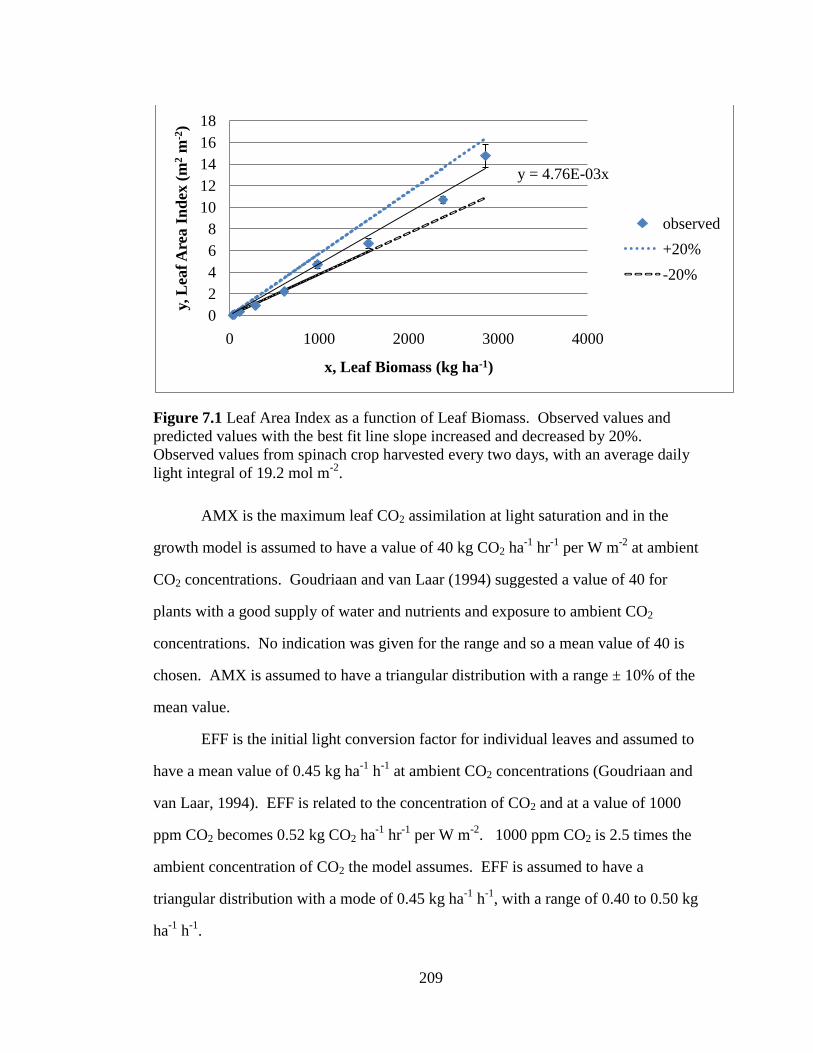
209
Figure 7.1 Leaf Area Index as a function of Leaf Biomass. Observed values and
predicted values with the best fit line slope increased and decreased by 20%.
Observed values from spinach crop harvested every two days, with an average daily
light integral of 19.2 mol m-2
.
AMX is the maximum leaf CO2 assimilation at light saturation and in the
growth model is assumed to have a value of 40 kg CO2 ha-1
hr-1
per W m-2
at ambient
CO2 concentrations. Goudriaan and van Laar (1994) suggested a value of 40 for
plants with a good supply of water and nutrients and exposure to ambient CO2
concentrations. No indication was given for the range and so a mean value of 40 is
chosen. AMX is assumed to have a triangular distribution with a range ± 10% of the
mean value.
EFF is the initial light conversion factor for individual leaves and assumed to
have a mean value of 0.45 kg ha-1
h-1
at ambient CO2 concentrations (Goudriaan and
van Laar, 1994). EFF is related to the concentration of CO2 and at a value of 1000
ppm CO2 becomes 0.52 kg CO2 ha-1
hr-1
per W m-2
. 1000 ppm CO2 is 2.5 times the
ambient concentration of CO2 the model assumes. EFF is assumed to have a
triangular distribution with a mode of 0.45 kg ha-1
h-1
, with a range of 0.40 to 0.50 kg
ha-1
h-1
.
y = 4.76E-03x
0
2
4
6
8
10
12
14
16
18
0 1000 2000 3000 4000
y, L
eaf
Are
a I
nd
ex (
m2
m-2
)
x, Leaf Biomass (kg ha-1)
observed
+20%
-20%
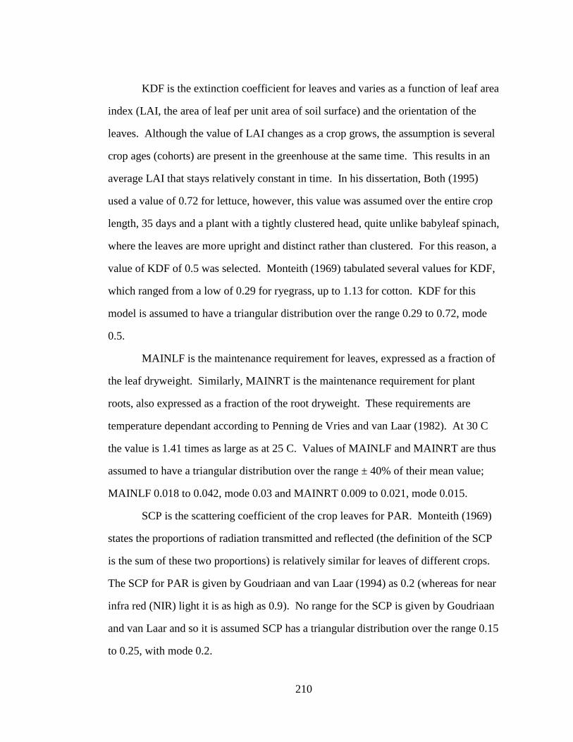
210
KDF is the extinction coefficient for leaves and varies as a function of leaf area
index (LAI, the area of leaf per unit area of soil surface) and the orientation of the
leaves. Although the value of LAI changes as a crop grows, the assumption is several
crop ages (cohorts) are present in the greenhouse at the same time. This results in an
average LAI that stays relatively constant in time. In his dissertation, Both (1995)
used a value of 0.72 for lettuce, however, this value was assumed over the entire crop
length, 35 days and a plant with a tightly clustered head, quite unlike babyleaf spinach,
where the leaves are more upright and distinct rather than clustered. For this reason, a
value of KDF of 0.5 was selected. Monteith (1969) tabulated several values for KDF,
which ranged from a low of 0.29 for ryegrass, up to 1.13 for cotton. KDF for this
model is assumed to have a triangular distribution over the range 0.29 to 0.72, mode
0.5.
MAINLF is the maintenance requirement for leaves, expressed as a fraction of
the leaf dryweight. Similarly, MAINRT is the maintenance requirement for plant
roots, also expressed as a fraction of the root dryweight. These requirements are
temperature dependant according to Penning de Vries and van Laar (1982). At 30 C
the value is 1.41 times as large as at 25 C. Values of MAINLF and MAINRT are thus
assumed to have a triangular distribution over the range ± 40% of their mean value;
MAINLF 0.018 to 0.042, mode 0.03 and MAINRT 0.009 to 0.021, mode 0.015.
SCP is the scattering coefficient of the crop leaves for PAR. Monteith (1969)
states the proportions of radiation transmitted and reflected (the definition of the SCP
is the sum of these two proportions) is relatively similar for leaves of different crops.
The SCP for PAR is given by Goudriaan and van Laar (1994) as 0.2 (whereas for near
infra red (NIR) light it is as high as 0.9). No range for the SCP is given by Goudriaan
and van Laar and so it is assumed SCP has a triangular distribution over the range 0.15
to 0.25, with mode 0.2.

211
Within the disease model the twelve parameters were estimated from different
data sources (outlined in chapter six). Unfortunately, there are no values for the
parameters of the disease model available in the literature, as the form of the model
and parameters were developed as a part of this dissertation.
The parameters examined are:
1. βconc, Concentration effect slope
2. αconc, Concentration effect intercept
3. εmycelium, Reference amount of mycelium @ 25 zoos ml-1
4. M0, Starting Mass of mycelium
5. βgrow, Mycelial growth rate slope
6. αgrow, Mycelial growth rate intercept
7. Amature, Maturation age of mycelium
8. ηphoto, Coefficient of Photosynthetic Rate reduction
9. βtemp, Temperature effect slope
10. αtemp, Temperature effect intercept
11. Arelease, Zoospore release age
12. Nzoos, Zoospore release amount
With the crop growth variables, assigning new random values for each cohort
was an obvious choice. With the disease variables, the selection of a time to assign
new random values is less clear. One possibility is to assign each crop cohort new
random disease variable values. However, as the disease generally takes more than
one crop generation to develop, assigning new values at this frequency would likely
result in an averaging of the disease variable values, and not produce the extreme
events required to cause failures in some of the production systems. Another
complicating factor is the temperatures which generally cause failures, usually only
occur during the summer months. As a compromise it was decided to select new

212
random values for the disease model at the beginning of every year and after every
crop failure. The annual change corresponds to a time when the nutrient solution
temperatures and subsequent disease pressures are least. The change after every crop
failure represents the breaking of the disease cycle through sterilization.
Seven of the parameters are a part of linear approximations for which there is
an associated slope and intercept. In the case of the concentration adjustment factors
(βconc and αconc) it was assumed that the values of slope and intercept are correlated,
and the equation for the concentration adjustment factor (originally equation 6.15) is
modified to:
𝐸(𝐶) = βconc ∗ log Zconc − log 25 zoos ml−1 + αconc
7.1
where: Zconc is the concentration of zoospores in solution (zoos ml-1
).
25 zoos ml-1
is the baseline concentration of zoospores.
The slope (βconc) was assumed to have a lognormal distribution with a mean of 0.180
and a coefficient of variation (CV) of 0.5. The intercept was also assumed to vary
lognormally with a mean of 1.0 and a CV of 0.5.
The mycelial growth rate parameters (βgrow and αgrow) were assumed to be
correlated. Rather than adjust the form of the equation (as was done for the
concentration parameters), triangular distributions were assumed for the minimum and
maximum observed mycelial growth rates (0.010 at 0.0 kg ha-1
uninfected root and
0.021 at 54.2 kg ha-1
uninfected root respectively). A common uniform random
variable was then used to generate a point on each distribution from which the slope
and intercept were then calculated. The minimum growth rate was assumed to have a
triangular distribution with a mean of 0.010 and limits of the mean ± 0.00325. The
maximum growth rate was assumed to have a triangular distribution with a mean of
0.021 and limits of the mean ± 0.0042.

213
The Coefficient of Photosynthetic Rate reduction (ηphoto) was assumed to have
a lognormal distribution with a mean of 0.79 and a CV of 0.5.
The temperature adjustment parameters (βtemp and αtemp) followed a similar
procedure as the mycelial growth rate to account for their correlation. A triangular
distribution with a mean of 0.58 and a range of ± 0.034 was assumed for the age
adjustment factor at 18C. A triangular distribution with a mean of 1.0 and a range of
0.042 was assumed for the age adjustment factor at 24C. A common uniform random
variable was then used to generate a point on each distribution, from which the slope
and intercept were then calculated.
εmycelium is the reference amount of mycelium @ 25 zoos ml-1
, or the amount of
mycelium formed on roots when exposed to a concentration of 25 zoos ml-1
in the
nutrient solution. Three values of εmycelium were estimated from Katzman‟s data (day1,
day 9 and day 14 inoculations) and were then averaged for a value of 3.23 kg
mycelium ha-1
. It was assumed εmycelium has a triangular distribution over the range of
the lowest to the highest εmycelium (0.71 to 6.75 kg mycelium ha-1
, mode 3.23 kg
mycelium ha-1
)
The starting mass of mycelia (M0) is a means of inoculating the crop with a
baseline amount of damage to simulate a naturally developing infection. It was
estimated by selecting a value that produced the observed level of damage in
Katzman‟s uninoculated control crops after 21 days. This parameter represents a
major simplification of the initial infection process and so the range of values should
represent uncertainty with the estimated value. For this reason a lognormal
distribution was assumed with a CV of 1.0 and µX = 1.95E-3 kg mycelium ha-1
.
The maturation age of mycelium, Amature, represents the age at which the
mycelial material begins to turn dark brown/black, whereas, the zoospore release age
(Arelease) represents the age the mycelia typically begin to release zoospores. Though

214
the values of these variables are assumed to be the same (128 hours) the probability
distributions are not. The maturation age of the mycelium was estimated from
observed data, whereas, the zoospore release ages were estimated as pairs of zoospore
release ages and zoospore release numbers that fit the data. The value of 128 hours for
the zoospore release age was selected to be the same as the Amature, because it is likely
the onset of dark brown black material represents the full reproductive cycle of
Pythium. The Amature was assumed to have a triangular distribution with an estimated
median value of 128 hours, a lower range of 104 hours and an upper range of 152
hours. The Arelease was assumed to have a triangular distribution, with a mode of 128
hours, an upper range of 168 hours and a lower range of 88 hours.
The zoospore release amount (nzoos) is the number of zoospores released per
kilogram of infected root material that achieved zoospore releasing age. After
reaching this age, the infected material releases a constant amount of zoospores per
kilogram per hour, as long as the infected material remains in solution. The estimate
for Nzoos was developed at the same time as the Arelease. The uncertainty of this
number is quite large and it should vary lognormally with a C.V. of 50% and a µx of
1.1E6 zoospores kg-1
mycelia.
The random number generator within Java was used to provide the random
numbers necessary for the Monte-Carlo simulation. These random numbers were
saved within a text file so common random numbers could be used for different
simulated production strategies. The random number generator provided a uniformly
distributed variable, whereas, the variability of some of the parameters, in the
simulation were assumed to be lognormal. To transform the uniformly distributed
random variables into lognormaly distributed random variables the Box-Muller
process was used to transform uniform variables to normal, which were then converted
to lognormal.

215
7.3.3 Implementation of Simulation Model
The simulation model was implemented in Java code to use the same language
as the previously coded greenhouse, growth and disease models. (Appendix A.)
7.4 RESULTS:
7.4.1 One pond system, controlled daily light integral
The results of the one pond system with light control (strict, time based harvest
schedule) are presented in Table 7.1, and Figure 7.2.
Table 7.1 Simulated mean time between Pythium outbreaks severe enough to require a
cleanout. For a multi-cohort one pond system with nutrient solution temperatures of
18C, 20C, 22C, 24C and uncontrolled, and crop durations of 12, 14 and 16 days with a
daily light integral of 17 mols m-2
PAR. (Simulation run for 500 years).
Nutrient
Solution
Temperature
(C)
Harvest
Age
(days)
Average
Harvest
dry mass
(kg ha-1)
Outbreaks Expected
Frequency of
Outbreaks
(outbreaks
year-1
)
Ratio to
uncontrolled
18 12 1186 16 0.032 0.11
18 14 1534 40 0.080 0.13
18 16 1885 77 0.154 0.10
20 12 1185 48 0.096 0.32
20 14 1534 93 0.186 0.30
20 16 1885 150 0.300 0.20
22 12 1185 94 0.188 0.64
22 14 1533 159 0.318 0.51
22 16 1883 337 0.674 0.46
24 12 1185 138 0.276 0.93
24 14 1532 306 0.612 0.98
24 16 1880 762 1.524 1.04
Uncontrolled 12 1090 148 0.296
Uncontrolled 14 1409 311 0.622
Uncontrolled 16 1721 736 1.472

216
Figure 7.2 Expected number of Pythium outbreaks per year, as a function of nutrient
solution temperature, and crop duration. For a one pond (multi-cohort) production
system with a daily light integral of 17 mols m-2
.
Clearly there is a benefit to using a lower nutrient solution temperature. As
would be expected, the longest crop duration examined (16 days) benefits most from a
reduced nutrient solution temperature. Comparing the 18 C, 16 day condition to the
uncontrolled, 16 day condition, the frequency of outbreaks was 9.5 times greater in the
uncontrolled condition. The 12 and 14 day conditions also benefited considerably
with improvements of 9.3 and 7.8 times, respectively. All of the temperature and crop
duration conditions examined showed a decrease in the frequency of outbreaks with a
reduction of temperature. The results of the uncontrolled nutrient solution temperature
conditions are quite similar to those where the temperature is controlled to 24C. This
is to be expected as the nutrient solution temperature tends to follow the air
temperature, and the setpoint for air temperature during the day is 24C (19C night).
Figure 7.3, Figure 7.4 and Figure 7.5 show the number of Pythium occurrences
by month for the 24C, 18C and uncontrolled nutrient solution temperatures, 16 day
crop duration conditions respectively.
0
0.2
0.4
0.6
0.8
1
1.2
1.4
1.6
1.8
12 14 16
Exp
ecte
d O
utb
reak
s p
er y
ear
Crop Duration (days)
18 C
20 C
22 C
24 C
uncontrolled
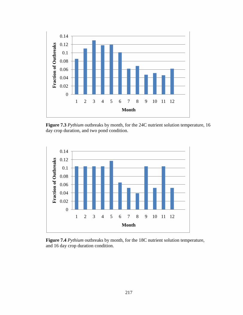
217
Figure 7.3 Pythium outbreaks by month, for the 24C nutrient solution temperature, 16
day crop duration, and two pond condition.
Figure 7.4 Pythium outbreaks by month, for the 18C nutrient solution temperature,
and 16 day crop duration condition.
0
0.02
0.04
0.06
0.08
0.1
0.12
0.14
1 2 3 4 5 6 7 8 9 10 11 12
Fra
ctio
n o
f O
utb
reak
s
Month
0
0.02
0.04
0.06
0.08
0.1
0.12
0.14
1 2 3 4 5 6 7 8 9 10 11 12
Fra
ctio
n o
f O
utb
reak
s
Month

218
Figure 7.5 Pythium outbreaks by month, for the uncontrolled nutrient solution
temperature, and 16 day crop duration condition.
The 24 and 18C conditions show a large negative skew, with more outbreaks
occurring earlier in the year than would be expected considering the nutrient
temperatures are maintained the same all year long. However, this is an artifact of the
simulation model where new disease parameters are assigned at the beginning of every
year. For this reason, the timing of Pythium infections is not examined further. An
investigation of the timing of Pythium infections throughout the year would require a
more complicated method of assigning variability to the Pythium disease parameters.
Such an analysis would be of little value as uncontrolled nutrient solution
temperatures are clearly not an option for commercial production of spinach.
7.4.2 Two pond system, controlled daily light integral
The results of the two pond system with light control (strict, time based harvest
schedule) are presented in Table 7.2. and Figure 7.6.
0
0.02
0.04
0.06
0.08
0.1
0.12
0.14
0.16
0.18
0.2
1 2 3 4 5 6 7 8 9 10 11 12
Fra
ctio
n o
f O
utb
reak
s
Month
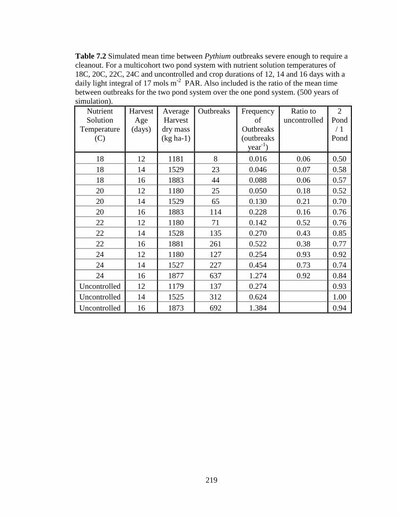
219
Table 7.2 Simulated mean time between Pythium outbreaks severe enough to require a
cleanout. For a multicohort two pond system with nutrient solution temperatures of
18C, 20C, 22C, 24C and uncontrolled and crop durations of 12, 14 and 16 days with a
daily light integral of 17 mols m-2
PAR. Also included is the ratio of the mean time
between outbreaks for the two pond system over the one pond system. (500 years of
simulation).
Nutrient
Solution
Temperature
(C)
Harvest
Age
(days)
Average
Harvest
dry mass
(kg ha-1)
Outbreaks Frequency
of
Outbreaks
(outbreaks
year-1
)
Ratio to
uncontrolled
2
Pond
/ 1
Pond
18 12 1181 8 0.016 0.06 0.50
18 14 1529 23 0.046 0.07 0.58
18 16 1883 44 0.088 0.06 0.57
20 12 1180 25 0.050 0.18 0.52
20 14 1529 65 0.130 0.21 0.70
20 16 1883 114 0.228 0.16 0.76
22 12 1180 71 0.142 0.52 0.76
22 14 1528 135 0.270 0.43 0.85
22 16 1881 261 0.522 0.38 0.77
24 12 1180 127 0.254 0.93 0.92
24 14 1527 227 0.454 0.73 0.74
24 16 1877 637 1.274 0.92 0.84
Uncontrolled 12 1179 137 0.274 0.93
Uncontrolled 14 1525 312 0.624 1.00
Uncontrolled 16 1873 692 1.384 0.94

220
Figure 7.6 Expected number of Pythium outbreaks per year, as a function of nutrient
solution temperature, and crop duration. For a two pond (multi-cohort) production
system with a daily light integral of 17 mols m-2
.
As in the case of the one pond system, there is a clear benefit to lower nutrient
solution temperatures on the occurrence of Pythium outbreaks. At lower temperatures
there is clearly a benefit to using a two pond system. For the case of a nutrient
solution temperature of 18 C, compared to an uncontrolled, in a 12 day crop cycle, the
expected frequency of Pythium outbreaks is 17 times smaller. Similar magnitudes of
improvement are also found in the 14 and 16 day crop cycles; 13.6 times and 15.7
times, respectively. When comparing the two pond system to the one system, it is
apparent that improvement in expected frequency of outbreaks is greater at lower than
higher temperatures. At 18C, the frequency of outbreaks is 0.5 to 0.57 of the one pond
system, whereas, with the 24C conditions, the frequency is 0.74 to 0.92 of the one
pond system. A reason for this difference is at higher temperatures there is a greater
chance of Pythium completing its reproductive cycle within the time the crop spends
0
0.2
0.4
0.6
0.8
1
1.2
1.4
1.6
12 14 16
Exp
ecte
d O
utb
reak
s p
er y
ear
Crop Duration (days)
18 C
20 C
22 C
24 C
uncontrolled

221
in the first pond. If the initial pond is subject to frequent outbreaks, the second
finishing pond is too. At lower temperatures the release of new zoospores is more
likely to be delayed until the cohorts are in the finishing pond, where the only other
cohorts to be infected are older and unable to infect material in the initial pond.
7.4.3 One pond system, natural daily light integral
The results of the one pond system with no light control (biomass based
harvest schedule) are presented in Table 7.3 and Figure 7.7.
Table 7.3 Simulated mean time between Pythium outbreaks severe enough to require a
cleanout. For a multicohort one pond system with nutrient solution temperatures of
18C, 20C, 22C, 24C and uncontrolled, and target crop harvest biomasses (kg dry mass
ha-1
) of 1186, 1534 and 1885 with no light integral control. (500 years of simulation).
Nutrient
Solution
Temperature
(C)
Harvest
Dry mass
(kg ha-1
)
Average
Harvest age
(days)
Outbreaks Frequency
of Outbreaks
(outbreaks
year-1
)
Ratio to
uncontrolled
18 1186 24 3940 7.9 0.54
18 1534 27 4748 9.5 0.60
18 1885 29 5378 10.8 0.67
20 1186 22 5740 11.5 0.78
20 1534 25 6501 13.0 0.82
20 1885 27 6899 13.8 0.86
22 1186 21 7379 14.8 1.01
22 1534 23 7950 15.9 1.01
22 1885 25 8081 16.2 1.01
24 1186 20 8829 17.7 1.20
24 1534 21 9084 18.2 1.15
24 1885 23 9127 18.3 1.14
Uncontrolled 1186 21 7339 14.7
Uncontrolled 1534 23 7887 15.8
Uncontrolled 1885 25 8019 16.0

222
Figure 7.7 Expected number of Pythium outbreaks per year, as a function of nutrient
solution temperature, and target crop harvest biomass. For a one pond (multi-cohort)
production system with no supplemental light (natural daily light integral).
The expected frequency of Pythium outbreaks is quite drastically different for
the conditions using harvesting triggered by biomass (with no supplemental lighting)
as opposed to a strict schedule with light control. Even with a nutrient solution of 18
C and the smallest harvest biomass considered, the estimated frequency of outbreaks is
8 per year. This is nearly 250 times greater than the corresponding schedule based
harvest condition. The frequency of outbreaks for the 24 C and smaller biomass
condition (1186 kg ha-1
) is only 2.2 times greater than the frequency for 18 C
condition.
7.4.4 Effect of daily light integral
The effect of varying the light integral the crops are grown under is illustrated
in Table 7.4 and Figure 7.8.
0
2
4
6
8
10
12
14
16
18
20
1186 1534 1885
Exp
ecte
d O
utb
reak
s p
er y
ear
Crop dry biomass (kg ha-1)
18 C
20 C
22 C
24 C
uncontrolled

223
Table 7.4 Effect of daily light integrals of 12, 17 and 22 mol m-2
on Pythium outbreak
frequency and harvest dry biomass, for a multi-cohort one pond system with a nutrient
solution temperature of 18C, and crop durations of 12, 14 and 16 days.
Daily Light Integral (mols m-2
)
12 17 22
Crop
duration
(days)
Outbreak
frequency
(outbreaks
year-1
)
Harvest
dry
Biomass
(kg ha-1
)
Outbreak
frequency
(outbreaks
year-1
)
Harvest
dry
Biomass
(kg ha-1
)
Outbreak
frequency
(outbreaks
year-1
)
Harvest
dry
Biomass
(kg ha-1
)
12 0.03 828 0.03 1186 0.03 1685
14 0.09 1094 0.08 1534 0.07 2140
16 0.17 1373 0.15 1885 0.14 2591
Figure 7.8 Effect of daily light integral (12, 17 and 22 mol m-2) on harvest dry
biomass with crop durations of 12, 14 and 16 days, in a multi-cohort one pond system
at 18C.
It is quite clear that increasing the duration of the crop increases the harvest
biomass. Extending the crop cycle from 12 to 16 days (33%) increases the dry
biomass by 66% with a daily light integral of 12 mols m-2
, and 54% with a daily light
integral of 22 mols m-2
. The relationship of light to harvest biomass is also clear.
Approximately doubling the daily light integral (12 to 22 mols m-2
) results in
approximately double the dry harvest biomass, regardless of the crop duration.
0
500
1000
1500
2000
2500
3000
12 14 16Harv
est
dry
bio
mass
(k
g h
a-1
)
Crop duration (days)
12 mols m-2
17 mols m-2
22 mols m-2

224
Changing the amount of light a crop receives has little effect on the frequency of
disease outbreak. There is a slightly greater frequency at the low light levels. This
difference is due to the fact that the factors controlling mycelium growth rate are the
same for both high and low light conditions, which should result in the same mass of
mycelia on each set of roots. However because the low light condition has a smaller
root mass (root mass is directly proportional to shoot mass), under certain conditions a
mass of mycelium on the low light roots can occupy enough of the roots to cause
wilting, that might not be enough to affect the larger roots of the high light condition.
7.5 DISCUSSION:
7.5.1 Overview of significant findings
The results of the simulation indicate there is a substantial decrease in the
frequency of Pythium outbreaks when lower nutrient solution temperatures are used.
In the one pond system of production, every two degrees Celsius drop approximately
halves the frequency. This trend holds for the three crop durations (12, 14 and 16 days
in pond) examined. Similar benefits are seen in the two pond system.
The benefits of reduced nutrient solution temperature are not as apparent when
the harvest schedule is controlled by the biomass of the crop, when no supplemental
lighting is used. Though the frequency of outbreaks approximately doubles between
the 18C and 24C conditions, these frequencies are on the order of several per year, and
are much larger than those observed in the supplemental light conditions. Clearly the
extended time taken to achieve target biomasses using natural light makes the crops
extremely susceptible to Pythium outbreaks.
There is also a clear benefit to reducing the time cohorts spend growing in the
pond. In the 18C nutrient solution conditions for both the one and two pond systems
with supplemental lighting, the frequency of outbreaks was reduced by approximately

225
66% for each two day reduction in crop length. This trend is also present at the higher
temperatures examined. The faster the crop can be grown, the better the chances are
of avoiding an outbreak.
Harvest biomass is directly proportional to the daily light integral the crop
receives. Doubling the daily light integral results in twice the harvest biomass.
Increasing the crop duration also increases the harvest biomass, the cost of which is an
increased risk of Pythium outbreak. Reduced light integral (and crop biomass) means
a smaller root mass, which in turn can make a crop more vulnerable to Pythium root
infections.
7.5.2 Limitations that affect validity/generalizability
A primary limitation for using the results of this study is it was developed from
data collected from experiments conducted with one pure strain of Pythium
aphanidermatum (selected for demonstrated virulence). Though random values for
the parameters describing the growth and development of Pythium were used to try to
encompass the variability among strains, other species of Pythium might not be
covered by that range. Specifically Pythium dissotocum has been identified as a
Pythium species found in lower temperature conditions (Bates and Stanghellini, 1984),
suggesting that its temperature optimum is lower than Pythium aphanidermatum. The
18C temperature condition effective against Pythium aphanidermatum, may not work
as well if Pythium dissotocum is present. In her analysis of the sources of Pythium in
greenhouse production, Katzman (2003) did not isolate Pythium dissotocum in the
Cornell greenhouses. However, this does not mean it is not present, nor that it cannot
be brought in. Further research is necessary to determine the values of the parameters
describing growth and development of Pythium dissotocum.

226
Another limitation to the model is it was assumed there are no ill effects from
physically moving a cohort from one pond to another. This assumption was made to
simplify the growth model. In lettuce production, during respacing there can be a
measurable impact on the growth rate, following moving of plants from one pond to
another. Further research is necessary to quantify the effects of moving plants from
pond to pond.
It is important to note the model assumes there is no effect of plant stress on
the effects of the disease. Should the crop be stressed by too much light, too high an
aerial temperature, mineral or oxygen deficiencies, they may become more vulnerable
to Pythium infection, resulting in a faster spread of the infection than would be
predicted. Disease work was conducted primarily in growth chambers with tightly
regulated environmental parameters, or in the greenhouse during the winter and spring
months where temperatures are under good control.
To simplify the simulation, no direct interaction between the crop growth
model and the greenhouse model was assumed. This assumption was justified by
having multiple cohorts in the pond at the same time, conditions remain relatively
constant throughout the simulation. Having many ages of the crop present at the same
time would tend to balance out the whole crop transpiration, and canopy radiation
properties.
The reliability of the components of the greenhouse were not considered.
Failures of equipment such as the cooling system, lights, pumps, nutrient treatment
systems and control hardware/software are likely to be noticed immediately
(Ferentinos 2002), or soon enough to not make a significant difference to the final
results of the analysis. The pond is a large heat reservoir and not susceptible to rapid
changes of temperature. An analysis of the failure modes of greenhouse components
was beyond the scope of this study.

227
7.5.3 Implications for application
One clear recommendation of this study is the justification for light integral
control. Harvesting on a predictable schedule is a benefit in itself, but supplemental
lighting under Ithaca, NY conditions is absolutely essential to ensure the crop spends
the minimum amount of time in the pond. Shading is also an important aspect of
integral control. Shading provides a consistent growth rate throughout the year, and
also helps protect the crop from excessive light levels and the higher temperatures and
stresses associated with them.
The results of this simulation are not intended as an accurate measure of the
risk involved with each production strategy, rather, the values of the results are in
comparing the risks of the different systems. Further, the model itself can provide
insight to a grower in developing their specific strategy for dealing with Pythium.
Careful examination of the roots of the crop should become a frequent activity in
hydroponic spinach production. Such inspections could identify a looming problem
and trigger strategies to avoid or minimize the effects of an outbreak. Browning of the
roots might trigger a grower to switch production to a two pond system until the
system cleans out. It is possible to envision complex production systems that make
use of the benefits of the systems examined in the study. The two pond system could
be further expanded into a three pond system, where one third of the crop growth is
spent in each pond. Or perhaps, a three pond system where the crop is moved out of
the first pond after 1/3 of its growth cycle when it is still small, and unentangled. It
would then go to a second pond where it would spend the remainder of its growth
cycle. The second finishing ponds would alternate (sharing the first pond as a
common source). If one of the secondary growth ponds showed signs of Pythium
damage the system would change to a true three pond system where material from the
228
uninfected second pond would be moved to the third pond until any infection cleans
up.
Implementing risk aversion strategies requires a financial investment by the
grower. Nutrient solution chillers must be purchased and sized based on expected
cooling loads. Supplemental lighting systems must be sized to provide an adequate
light level, which is specific to the location and construction of the greenhouse. Extra
labor and materials costs are required for a two pond system, as is more frequent
harvesting on shorter crop cycles. All of these factors need to be taken into
consideration when growers are formulating spinach production systems that suit their
particular needs.

229
CHAPTER 8: CONCLUSIONS
Pythium aphanidermatum has been identified as the primary roadblock to
commercial production of hydroponic spinach. To address this issue, Katzman (2003)
examined the effects of temperature, inoculum concentration and timing on the
development and spread of the disease. Continuing with this work, NYSERDA
commissioned a study to identify treatment techniques to remove Pythium from the
nutrient solution (Albright et al., 2007). This information forms the basis for this
dissertation, the primary objective of which is to quantitatively compare the risk of
Pythium outbreak in different hydroponic baby spinach production systems. Such
information could be used by a potential grower to select a system suitable for their
risk comfort level, financial and physical conditions. An additional use of this thesis
is the identification of production systems that warrant further investigation/validation.
To achieve this objective a number of tasks were undertaken. These tasks,
with any associated conclusions, are as follow:
1. To investigate current and non-traditional techniques for the control of
Pythium aphanidermatum in hydroponic nutrient solutions.
Chapter two of this dissertation describes development of a seedling bioassay to
quickly determine the effectiveness of different nutrient solution treatment techniques.
The bioassay allowed a quantitative comparison of the four techniques selected for
examination; electrochemical, thermal, sonic and ultraviolet sterilization. All of the
techniques investigated proved capable of some reduction in the concentration of
zoospores in solution, with sonication providing the best performance; however,
Electrochemical treatment was found to be largely ineffective.
Following this initial test of treatment technologies, ultraviolet sterilization,
and filtration were selected for further hydroponic production testing. These

230
technologies were selected for their effectiveness in removing zoospores from solution
and the ease of adapting them to in-line flow use. Chapter three of this dissertation
presents the results of continuous multi-cohort production with the two active
treatment techniques (UV and filtration) and a passive technique of reducing the
nutrient solution temperature. The conclusions of this chapter were that:
Inline treatment of the nutrient solution was ineffective in controlling
Pythium zoospore damage in pond production. Filtration and UV failed to
prevent the migration of zoospores from infected material. UV treatment
negatively affected uninoculated plants by destroying the chelator used to
keep iron soluble.
Reducing the nutrient solution temperature to 20C was an effective means
of halting the spread of disease in a 14 day crop cycle. By increasing the
time it takes for Pythium to develop and reproduce, it is possible to harvest
and remove infected material before it has a chance to release zoospores.
2. To apply the findings of the solution treatment techniques in the development
of production strategies.
Temperature reduction of the nutrient solution was shown to be an effective means
of controlling Pythium aphanidermatum in pond production. Reduced temperatures
were shown by Katzman (2003) to slow the growth and reproductive rate of Pythium
a. By increasing the reproductive cycle of Pythium a. to longer than the crop cycle,
any infected plants were harvested/removed before having an opportunity to release
zoospores and further spread the infection. One temperature (20C) and one crop
duration (14 days) was investigated in chapter three. Other temperatures selected for
further investigation were, 18C, 20C, 22C, 24C and uncontrolled (naturally occurring).
Coupled within these temperatures, crop durations of 12, 14 and 16 days were

231
selected. These temperature and duration combinations represent the likely range of
options that a grower would select.
A further development investigated the use of two ponds. Cohorts older than
half the crop duration are placed in a second “finishing” pond. Any zoospore release
in the second pond would not infect material in the initial starting pond. Thus an
infection in the initial pond would hopefully die out faster than in a single pond. Once
the initial pond has cleaned itself, the material moving to the second pond should also
be clean.
A third aspect of production strategy investigated was the use of daily light
integral control. Integral control provides a consistent amount of light to the crop
through supplemental lighting and shading. This control provides a consistent amount
of growth year round, and allows harvesting on a set time schedule, as opposed to
natural lighting only where harvesting is performed when the crop reaches an
acceptable size.
The conclusions of chapter three were that:
because nutrient solution temperature is so important to the development of
Pythium, temperatures of 18, 20, 22 and 24 would be investigated, along with
an uncontrolled temperature condition,
the longer a crop spends in a pond, the greater the risk of Pythium completing
its reproductive cycle and causing a new outbreak, and so crop durations of 12,
14 and 16 days in pond were investigated, both with one and two pond
systems,
the use of supplemental lighting and shading ensures a predictable harvest
schedule, and to investigate this importance from a disease perspective, the
model was run without light integral control and harvests conducted when the
crop reached target biomasses.
232
3. To develop a linked greenhouse, crop, and disease model to better understand
the dynamics of a Pythium aphanidermatum infection and to simulate and
evaluate different production strategies.
Chapters four, five and six detail development of a greenhouse simulation model, a
hydroponic spinach production model, and a Pythium disease model. The greenhouse
simulation uses the assumption of stepwise steady state heat and moisture flow within
a greenhouse to estimate temperatures of layers within the greenhouse. Specifically it
is capable of predicting nutrient solution and aerial temperatures based on outdoor air
temperature, relative humidity, and solar radiation. The spinach growth model adapts
the SUCROS framework for hourly prediction of spinach growth within a greenhouse
equipped with supplemental lighting. The Pythium disease model was developed from
observations made by Katzman (2003). Specifically it tracks the mass of mycelium
present on each cohort of spinach, and predicts the timing and spread of the infection
to other cohorts. Damage to the roots by the mycelium affects the growth of the
spinach crop. As the spread and development of Pythium is highly temperature
dependent, the greenhouse simulation model was necessary to predict effects of
common greenhouse environmental controls on the nutrient solution and aerial
temperatures, as well as level of supplemental light.
The conclusions of chapters four, five and six were that:
though lacking direct data to validate the greenhouse simulation model, the
values predicted are within reason, and are typical of observed conditions,
the mechanistically based SUCROS spinach growth model predicts growth
with reasonable accuracy and provides a good means of scaling growth based
on damage to disease,
233
the Pythium disease model developed from Katzman‟s (2003) data reasonably
predicts the observed development and spread of Pythium aphanidermatum in
multi-cohort pond production.
4. To simulate production strategies using the greenhouse crop disease model to
develop expected risk profiles for each strategy.
To simulate different production strategies, distributions were assumed for each of the
seven spinach growth, and twelve Pythium disease model variables. Monte-Carlo
simulation was then used to model Pythium outbreaks. The results of the simulations
were estimates of the frequency of Pythium outbreak. The conclusions of chapter
seven were:
The simulation suggests that every two degree drop in the nutrient solution,
approximately halves the frequency of Pythium outbreak within the
temperature range of 18C to 24C,
every two day reduction of the amount of time the crop spends in pond,
approximately halves the frequency of Pythium outbreaks, within the crop
production range of 12 to 16 days,
a two pond system can also approximately halve the frequency of outbreaks,
but only at a temperature of 18C. Outbreak frequency increases with
increasing temperature until there is no difference between a one and two pond
system at 24C,
at the highest temperature investigated, 24C, there was little difference
between a one and two pond system,
light integral control was essential to the successful production of spinach.
Production strategies that relied on natural light failed rapidly, with outbreak

234
frequencies on the order of several per year, as opposed to fractions per year,
observed in the other conditions with light integral control.
The productivity of spinach crops is directly proportional to the amount of
light the crop receives. Doubling the amount of light a crop receives over its
growth cycle, doubles the harvest biomass. Similarly lengthening the growth
cycle increases the harvest biomass (at the cost of increasing the risk of
Pythium outbreak.)

235
APPENDIX
The appendix contains a listing of most of the functions used in the greenhouse,
spinach disease and production models. Code relating to the graphical user interface
(GUI) was not included. Another omission for reasons of copyright protection is the
coding of the Light and Shade System Implementation (LASSI).
// Functions used for the Greenhouse Simulation model
//********************************************************************
//********************************************************************
private double[][] getDataArray(int nPoints){
// Initialize data arrays
double[][] greenhouseData = new double[nPoints+1][21];
double[] newTempsAndConds = new double[18];
double[] tempsCondsTm1 = new double[18];
double[] ctrlStatus = new double[6];
double[] enviroConds = new double[4];
double[][] enviroData = new double[9000][3];
double[] times = new double[2];
double[] lightData = new double[20];
double[] cropParams = new double[20];
double[] canopyRadProfileVals = new double[7];
double[] aboveCanopyRadiationVals = new double[4];
double[] solarRadiationParams = new double[12];
double[] lightingVals = new double[6];
double[] transmissivities = new double[2];
double[] CO2LASSIsets = new double[3];
double[] LASSISets = new double[5];
// Initialize variables
double convertToMols = 2.08135E-6; // Mol/m2 / J/m2
double ambCO2 = 400.0; // ambient CO2 concentration ppm
double LAT = 42.3; // latitude of Ithaca, NY
double day = 0; // julian day
double time = 0; // hour of the day (0 to 23)
double sunriseHour;
double sunsetHour;
// Initial conditions:
double tSoilInf = 9.88 + 273.15;
double tSoilTm1 = 12.54 + 273.15;
double tConcreteTm1 = 19.55 + 273.15;
double tWaterTm1 = 20.10 + 273.15;
double tMediaTm1 = 19.33 + 273.15;
double tSurfaceTm1 = 19.21 + 273.15;
236
double tCropTm1 = 18.38 + 273.15;
double tGH1AirTm1 = 19.0 + 273.15;
double tShadeTm1 = 16.23 + 273.15;
double tGH2AirTm1 = 14.20 + 273.15;
double tGlassTm1 = 12.16 + 273.15;
double tAmbient = 5 + 273.15;
double thetaSun = 0;
double tSky = 5 + 273.15;
double tGHAirTm1 = tGH1AirTm1;
double humAmbient = 0.4;
double humGH1AirTm1 = 0.4;
double humGHAirTm1 = 0.4;
double humGH2AirTm1 = 0.4;
double ventRate = Double.parseDouble(jTextField11.getText()) * AREA;
double qHeater = 0.0;
double infilRate = 0.0;
tempsCondsTm1[0] = tSoilTm1;
tempsCondsTm1[1] = tConcreteTm1;
tempsCondsTm1[2] = tWaterTm1;
tempsCondsTm1[3] = tMediaTm1;
tempsCondsTm1[4] = tSurfaceTm1;
tempsCondsTm1[5] = tCropTm1;
tempsCondsTm1[6] = tGH1AirTm1;
tempsCondsTm1[7] = tShadeTm1;
tempsCondsTm1[8] = tGH2AirTm1;
tempsCondsTm1[9] = tGlassTm1;
tempsCondsTm1[10] = tSoilInf;
tempsCondsTm1[11] = tGHAirTm1;
tempsCondsTm1[12] = humGHAirTm1;
tempsCondsTm1[13] = humGH1AirTm1;
tempsCondsTm1[14] = humGH2AirTm1;
tempsCondsTm1[15] = ventRate;
tempsCondsTm1[16] = qHeater;
tempsCondsTm1[17] = infilRate;
times[0] = day;
times[1] = time;
lightData[0] = 0; // current light intensity (umol/s)
lightData[1] = 0; // sumTotalPPF (Mols/m2)
lightData[2] = 0; // lightsOn? (double)
lightData[3] = 0; // shadesOpen? (double)
lightData[4] = 17; // target Moles
lightData[5] = 42; // latitude
lightData[6] = 0.7; // transMVTY
lightData[7] = 0.5; // shadeFactor
lightData[8] = 180; // amount of mol PPF/time supp. lights provide
lightData[9] = 0.0036; // microMol/m^2/s PPF provided by lights
lightData[10] = 22; // offpeak start
lightData[11] = 7; // offpeak end
lightData[12] = 0.0; // sumSolarPPF (Mols/m2)
lightData[13] = 400.0; // target CO2 concentration (ppm)
lightData[14] = 0.0; // average light level past hour
lightData[15] = 0.0; // estimated outdoor temperature next hour

237
lightData[16] = 0.0; // sunriseHour
lightData[17] = 0.0; // sunsetHour
lightData[18] = 400.0; // ambient CO2 concentration (ppm)
lightData[19] = 0.55; // percentage of sunlight that is PAR
ctrlStatus[0] = 0; // lighting on? 1 for 0, 0 for off
if (jToggleButton4.isSelected()) ctrlStatus[1] = 1; // shade closed?
else ctrlStatus[1] = 0;
if (jToggleButton2.isSelected()) ctrlStatus[2] = 1; // pad cooling
else ctrlStatus[2] = 0;
ctrlStatus[3] = 0; // heat output by the lights
enviroConds[0] = tAmbient;
enviroConds[1] = humAmbient;
enviroConds[2] = thetaSun;
enviroConds[3] = tSky;
// input the first data value (initial conditions) into the temperature array
greenhouseData[0][0] = tSoilInf;
greenhouseData[0][1] = tSoilTm1;
greenhouseData[0][2] = tConcreteTm1;
greenhouseData[0][3] = tWaterTm1;
greenhouseData[0][4] = tMediaTm1;
greenhouseData[0][5] = tSurfaceTm1;
greenhouseData[0][6] = tCropTm1;
greenhouseData[0][7] = tGH1AirTm1;
greenhouseData[0][8] = tShadeTm1;
greenhouseData[0][9] = tGH2AirTm1;
greenhouseData[0][10] = tGlassTm1;
greenhouseData[0][11] = tAmbient;
greenhouseData[0][12] = tSky;
greenhouseData[0][13] = ventRate;
greenhouseData[0][14] = qHeater;
greenhouseData[0][15] = thetaSun;
greenhouseData[0][16] = 0;
greenhouseData[0][17] = 0;
greenhouseData[0][18] = 0;
greenhouseData[0][19] = 400;
greenhouseData[0][20] = 400;
tSetpoint = 24 + 273.15;
controlOn = true;
enviroData = readDataFile("G:\\ITHACA85to97.TXT",1);
for (int i = 1; i < (nPoints + 1); i ++){
// if/else to maintain 0-24 hour loop
if( time>=0 && time<=22) {
time++; // increment an hour for each loop
} // end if
else {

238
time = 0; // resets hour back to 0 (midnight) if previously 11 pm
day++; // increments day to reflect 24 hour period
} // end else
times[0] = day;
times[1] = time;
sunriseHour = Math.floor(calculateSunVals(day,42)[0]);
sunsetHour = Math.floor(calculateSunVals(day,42)[1]);
transmissivities = calculateTransmissivity(times,sunriseHour,sunsetHour);
lightData[16] = sunriseHour;
lightData[17] = sunsetHour;
// using real data?
if (true){
enviroConds[0] = enviroData[i][0];
enviroConds[1] = enviroData[i][1];
enviroConds[2] = enviroData[i][2];
enviroConds[3] = calculateTSky(enviroConds[0]);
} // end if
// using Light/Shade Control?
if (true){
lightData[0] = enviroConds[2]*convertToMols; // current light intensity
// Decide whether to use regular or CO2 supplemented LASSI
if (false) {
// provide CO2LASSI with lightData array, time, day, current CO2 concentration, and
//next hours outdoor temp
CO2LASSIsets = CO2LASSI2(lightData, time, day, lightData[18], enviroData[i+1][0]-
273.15);
lightData[2] = CO2LASSIsets[0];
lightData[3] = CO2LASSIsets[1];
lightData[13] = CO2LASSIsets[2];
if (CO2LASSIsets[3] == 1){
lightData[18] = lightData[13];
} // end if
else {
lightData[18] = ( lightData[18] - ambCO2 ) * Math.exp( -CO2LASSIsets[4] ) +
ambCO2;
} // end else
// update the solarPAR recieved and the totalGrowth
if (lightData[3] == 1){
lightData[12] = lightData[12] +
enviroConds[2]*lightData[19]*convertToMols*lightData[6]*transmissivities[0];
lightData[1] = lightData[1] +
(enviroConds[2]*lightData[19]*convertToMols*lightData[6]*transmissivities[0] +
lightData[2] * lightData[8] * lightData[9])
* ((Math.log(2.66E4) - Math.log(400)) / (Math.log(2.66E4) -
Math.log(lightData[13])));
} // end if

239
else {
lightData[12] = lightData[12] +
enviroConds[2]*lightData[19]*convertToMols*lightData[6]*transmissivities[0];
lightData[1] = lightData[1] +
(enviroConds[2]*lightData[19]*convertToMols*lightData[6]*transmissivities[0]*
lightData[7] + lightData[2] * lightData[8] * lightData[9])
* ((Math.log(2.66E4) - Math.log(400)) / (Math.log(2.66E4) -
Math.log(lightData[13])));
} // end else
if (CO2LASSIsets[1] == 0) ctrlStatus[1] = 1; // shade closed?
else ctrlStatus[1] = 0;
if (CO2LASSIsets[0] == 0) ctrlStatus[0] = 0; // lightsON?
else ctrlStatus[0] = 1;
} // end if
else {
LASSISets = LASSI(sunriseHour, sunsetHour, time, day, lightData);
lightData[2] = LASSISets[0];
lightData[3] = LASSISets[1];
// update the solarPAR recieved and the totalGrowth
if (lightData[3] == 1){
lightData[12] = lightData[12] +
enviroConds[2]*lightData[19]*convertToMols*lightData[6]*transmissivities[0];
lightData[1] = lightData[1] +
(enviroConds[2]*lightData[19]*convertToMols*lightData[6]*transmissivities[0] +
lightData[2] * lightData[8] * lightData[9]);
} // end if
else {
lightData[12] = lightData[12] +
enviroConds[2]*lightData[19]*convertToMols*lightData[6]*transmissivities[0]*
lightData[7];
lightData[1] = lightData[1] +
(enviroConds[2]*lightData[19]*convertToMols*lightData[6]*transmissivities[0]*
lightData[7]
+ lightData[2] * lightData[8] * lightData[9]);
} // end else
if (LASSISets[1] == 0) ctrlStatus[1] = 1; // shade closed?
else ctrlStatus[1] = 0;
if (LASSISets[0] == 0) ctrlStatus[0] = 0; // lightsON?
else ctrlStatus[0] = 1;
} // end if
} // end if
else{
lightData[1] = lightData[1] +
enviroConds[2]*lightData[19]*convertToMols*lightData[6]*transmissivities[0];
} // end else

240
// check for closing shades at night (Irrespective of LASSI)
if (true){
if ((time > calculateSunVals(day, 42)[1]) || ( time < calculateSunVals(day,42)[0])){
ctrlStatus[1] = 1;
} // end if
} // end if
// using temperature control?
if (controlOn){
if (( i%24 >= sunriseHour) && (i%24 <= sunsetHour)){
tSetpoint = daysetpoint + 273.15;
} // end if
else{
tSetpoint = nightsetpoint + 273.15;
} // end else
newTempsAndConds = determineHeatingVenting(tempsCondsTm1, ctrlStatus,
enviroConds);
} // end if
else{
tempsCondsTm1[15] = 0.0;
tempsCondsTm1[16] = 0.0;
newTempsAndConds = calculateNewTemps(tempsCondsTm1, ctrlStatus, enviroConds);
} // end else
greenhouseData[i][0] = newTempsAndConds[10];
greenhouseData[i][1] = newTempsAndConds[0];
greenhouseData[i][2] = newTempsAndConds[1];
greenhouseData[i][3] = newTempsAndConds[2];
greenhouseData[i][4] = newTempsAndConds[3];
greenhouseData[i][5] = newTempsAndConds[4];
greenhouseData[i][6] = newTempsAndConds[5];
greenhouseData[i][7] = newTempsAndConds[6];
greenhouseData[i][8] = newTempsAndConds[7];
greenhouseData[i][9] = newTempsAndConds[8];
greenhouseData[i][10] = newTempsAndConds[9];
greenhouseData[i][11] = enviroConds[0];
greenhouseData[i][12] = enviroConds[3];
greenhouseData[i][13] = newTempsAndConds[15];
greenhouseData[i][14] = newTempsAndConds[16];
greenhouseData[i][15] = enviroConds[2];
greenhouseData[i][16] = lightData[3];
greenhouseData[i][17] = lightData[2];
greenhouseData[i][18] = lightData[1];
greenhouseData[i][19] = lightData[13];
greenhouseData[i][20] = lightData[18];
tempsCondsTm1 = newTempsAndConds;
// reset the daily light integral (total and solar)
if (time == Math.floor(sunriseHour)){
lightData[1] = 0;
lightData[12] = 0;
}// end if

241
} // end for loop through hours (end i)
// Output the results of the simulation to a text file
try{
// Create file
FileWriter fstream = new FileWriter("g:\\greenhouseOut.txt");
BufferedWriter out = new BufferedWriter(fstream);
double shadeclosed = 0;
for (int y = 1; y < greenhouseData.length; y++){
if (greenhouseData[y][16] == 0.0) shadeclosed = 1;
else shadeclosed = 0;
out.write( (greenhouseData[y][1]-273.15) + "\t" +
(greenhouseData[y][2]-273.15) + "\t" +
(greenhouseData[y][3]-273.15) + "\t" +
(greenhouseData[y][4]-273.15) + "\t" +
(greenhouseData[y][5]-273.15) + "\t" +
(greenhouseData[y][6]-273.15) + "\t" +
(greenhouseData[y][7]-273.15) + "\t" +
(greenhouseData[y][8]-273.15) + "\t" +
(greenhouseData[y][9]-273.15) + "\t" +
(greenhouseData[y][10]-273.15) + "\t" +
(greenhouseData[y][17]) + "\t" +
(shadeclosed) + "\t" +
(greenhouseData[y][11]) + "\t" +
(greenhouseData[y][15]) + "\r\n");
} // end for
//Close the output stream
out.close();
}catch (Exception e){//Catch exception if any
System.err.println("Error: " + e.getMessage());
} // end catch
return greenhouseData;
}
//////////////////////////////////////////////////////////////////////////////////////////////////////////////////////////////////////////////////////
private double[] searchHeating(double hiRate, double lowRate, double[] tempsCondsTm1, double[]
ctrlStatus, double[] enviroConds) {
// search for optimal heating rate between two specified levels using bisection
double[] newTempsAndConds = tempsCondsTm1;
double avgRate = 0.0;
double tAirLow = 0.0;
double tAirHigh = 0.0;
double tAirAvg = 0.0;
do {
tempsCondsTm1[16] = lowRate;
newTempsAndConds = calculateNewTemps(tempsCondsTm1, ctrlStatus, enviroConds);
242
tAirLow = newTempsAndConds[6];
tempsCondsTm1[16] = hiRate;
newTempsAndConds = calculateNewTemps(tempsCondsTm1, ctrlStatus, enviroConds);
tAirHigh = newTempsAndConds[6];
avgRate = (hiRate + lowRate)/2;
tempsCondsTm1[16] = avgRate;
newTempsAndConds = calculateNewTemps(tempsCondsTm1, ctrlStatus, enviroConds);
tAirAvg = newTempsAndConds[6];
if (tAirAvg < tSetpoint){
lowRate = avgRate;
}
else {
hiRate = avgRate;
}
} while ( Math.abs(tAirLow - tAirHigh) > tTolerance);
return newTempsAndConds;
} // end searcgHeating
private double[] searchVenting(double hiRate, double lowRate, double[] tempsCondsTm1, double[]
ctrlStatus, double[] enviroConds) {
// search for optimal venting rate between two specified levels using bisection
double[] newTempsAndConds = tempsCondsTm1;
double avgRate = 0.0;
double tAirLow = 0.0;
double tAirHigh = 0.0;
double tAirAvg = 0.0;
do {
tempsCondsTm1[15] = lowRate;
newTempsAndConds = calculateNewTemps(tempsCondsTm1, ctrlStatus, enviroConds);
tAirLow = newTempsAndConds[6];
tempsCondsTm1[15] = hiRate;
newTempsAndConds = calculateNewTemps(tempsCondsTm1, ctrlStatus, enviroConds);
tAirHigh = newTempsAndConds[6];
avgRate = (hiRate + lowRate)/2;
tempsCondsTm1[15] = avgRate;
newTempsAndConds = calculateNewTemps(tempsCondsTm1, ctrlStatus, enviroConds);
tAirAvg = newTempsAndConds[6];
if (tAirAvg < tSetpoint){
hiRate = avgRate;
}
else {
lowRate = avgRate;
}
} while ( Math.abs(tAirLow - tAirHigh) > tTolerance);
return newTempsAndConds;
} // end searchVenting
//////////////////////////////////////////////////////////////////////////////////////////////////////////////////////////////////////////////////////

243
private double[] determineHeatingVenting(double[] tempsCondsTm1, double[] ctrlStatus, double[]
enviroConds){
double[] newTempsAndConds = new double[17];
double tMaxVent = 0.0;
double tMaxHeat = 0.0;
double tNoHeatVent = 0.0;
//check to determine if either the heating system or venting system needs to be maxed out
tempsCondsTm1[15] = MAXVENTRATE;
tempsCondsTm1[16] = 0.0;
newTempsAndConds = calculateNewTemps(tempsCondsTm1, ctrlStatus, enviroConds);
tMaxVent = newTempsAndConds[6];
if (tMaxVent > tSetpoint + tTolerance){
return newTempsAndConds;
}
tempsCondsTm1[15] = 0.0;
tempsCondsTm1[16] = QHEATERMAX;
newTempsAndConds = calculateNewTemps(tempsCondsTm1, ctrlStatus, enviroConds);
tMaxHeat = newTempsAndConds[6];
if (tMaxHeat < tSetpoint - tTolerance){
return newTempsAndConds;
}
// At this point of the code must be within a range that can be affected by a control Action
// determine what happens without either heating or cooling
tempsCondsTm1[15] = 0.0;
tempsCondsTm1[16] = 0.0;
newTempsAndConds = calculateNewTemps(tempsCondsTm1, ctrlStatus, enviroConds);
tNoHeatVent = newTempsAndConds[6];
if (tNoHeatVent >= tSetpoint + tTolerance){
// Need to search for venting rate
newTempsAndConds = searchVenting(MAXVENTRATE, 0.0, tempsCondsTm1, ctrlStatus,
enviroConds);
}
else {
// Need to search for heating rate
newTempsAndConds = searchHeating(QHEATERMAX, 0.0, tempsCondsTm1, ctrlStatus,
enviroConds);
}
return newTempsAndConds;
} // end determineHeatingVenting
//////////////////////////////////////////////////////////////////////////////////////////////////////////////////////////////////////////////////////
private double[] calculateNewTemps(double[] previousTempsAndConds, double[] greenhouseConts,
double[] ambientConds){
// the array of temperatures humidities, and heat/vent rates to return
double newTempsAndConds[] = new double[18];
tSoilTm1 = previousTempsAndConds[0];
tConcreteTm1 = previousTempsAndConds[1];
tWaterTm1 = previousTempsAndConds[2];

244
tMediaTm1 = previousTempsAndConds[3];
tSurfaceTm1 = previousTempsAndConds[4];
tCropTm1 = previousTempsAndConds[5];
tGH1AirTm1 = previousTempsAndConds[6];
tShadeTm1 = previousTempsAndConds[7];
tGH2AirTm1 = previousTempsAndConds[8];
tGlassTm1 = previousTempsAndConds[9];
tSoilInf = previousTempsAndConds[10];
tGHAirTm1 = previousTempsAndConds[11];
humGHAirTm1 = previousTempsAndConds[12];
humGH1AirTm1 = previousTempsAndConds[13];
humGH2AirTm1 = previousTempsAndConds[14];
ventRate = previousTempsAndConds[15];
qHeater = previousTempsAndConds[16];
infilRate = previousTempsAndConds[17];
if (greenhouseConts[0] == 1) lightsOn = true;
else lightsOn = false;
if (greenhouseConts[1] == 1) shadesClosed = true;
else shadesClosed = false;
if (greenhouseConts[2] == 1) padsOn = true;
else padsOn = false;
tAmbient = ambientConds[0];
humAmbient = ambientConds[1];
thetaSun = ambientConds[2];
tSky = ambientConds[3];
psychroAmb = calculatePsychroVals(tAmbient, humAmbient, Patm);
WAmb = psychroAmb[5];
VsaAmb = psychroAmb[6];
enthalpyAmb = psychroAmb[7];
rhoAmb = psychroAmb[8];
// set conditions of the incoming air from vent if the evaporative cooling pads are on
if (padsOn){
psychroVent = calculateStateOfAirFromPad(psychroAmb, 0.75);
tVentAir = psychroVent[0];
WVent = psychroVent[5];
VsaVent = psychroVent[6];
}
else {
psychroVent = psychroAmb;
tVentAir = psychroAmb[0];
WVent = psychroAmb[5];
VsaVent = psychroAmb[6];
}
// Based on whether the shades are open or not solve for temps using the shade model or not
if (!shadesClosed){
// arrays to hold linear equations
Matrix a = new Matrix(new double[8][8]);
Matrix b = new Matrix(new double[8][1]);
Matrix X = new Matrix(new double[8][1]);
245
psychroGHTm1 = calculatePsychroVals(tGHAirTm1, humGHAirTm1, Patm);
WGHTm1 = psychroGHTm1[5];
VsaGHTm1 = psychroGHTm1[6];
enthalpyGHTm1 = psychroGHTm1[7];
rhoGHTm1 = psychroGHTm1[8];
VGH = AREA * ZGHAIR;
thetaGlass = thetaSun*glassTrans*AREA; // Sunlight level after passing through glass
enviroVals[0] = thetaGlass + thetaL; // Net all wave Radiation reaching canopy W/m2
enviroVals[1] = (1-CANOPYREFL)*(thetaGlass+thetaL)*Math.exp(-
1*K*LAI)*ALPHAM;
enviroVals[2] = 0.12; // air speed at height of 2m, m/s
evapoTranspiration = calculateEvapoTranspiration(psychroGHTm1, enviroVals, tCropTm1,
AREA);
WGH = (((WAmb/VsaAmb)*infilRate + (WVent/VsaVent)*ventRate + evaporation[0] +
evapoTranspiration[0] + (WGHTm1/VsaGHTm1)*VGH)/(VGH + ventRate +
infilRate))*VsaGHTm1;
tSurfCropAvgCubed = Math.pow(((tSurfaceTm1 + tCropTm1) / 2),3);
tSurfGlassAvgCubed = Math.pow(((tSurfaceTm1 + tGlassTm1) / 2),3);
tGlassCropAvgCubed = Math.pow(((tGlassTm1 + tCropTm1) / 2),3);
tGlassSkyAvgCubed = Math.pow(((tGlassTm1 + tSky) / 2),3);
// energy balance soil layer
a00 = -1 * (1/(ZSOIL/KASOIL + ZCONCRETE/KACONCRETE) + KASOIL/(ZSOIL/2) +
TMASSSOIL);
a01 = 1/(ZSOIL/KASOIL + ZCONCRETE/KACONCRETE);
b0 = -1 * ((KASOIL/(ZSOIL/2))*tSoilInf + TMASSSOIL*tSoilTm1);
a.set(0,0,a00);
a.set(0,1,a01);
b.set(0,0,b0);
// energy balance concrete layer
a10 = 1/(ZSOIL/KASOIL + ZCONCRETE/KACONCRETE);
a11 = -1 * (HAWATER + (1/(ZSOIL/KASOIL + ZCONCRETE/KACONCRETE)) +
TMASSCONCRETE);
a12 = HAWATER;
b1 = -1 * (TMASSCONCRETE * tConcreteTm1);
a.set(1,0,a10);
a.set(1,1,a11);
a.set(1,2,a12);
b.set(1,0,b1);
// energy balance water layer
a21 = HAWATER;
a22 = -1 * (2*HAWATER + TMASSWATER);
a23 = HAWATER;
b2 = -1 * (TMASSWATER * tWaterTm1 + PUMPHEAT);
a.set(2,1,a21);
a.set(2,2,a22);
a.set(2,3,a23);

246
b.set(2,0,b2);
// energy balance media layer
a32 = HAWATER;
a33 = -1 * (KAMEDIA/(ZMEDIA/2) + HAWATER + TMASSMEDIA);
a34 = KAMEDIA/(ZMEDIA/2);
b3 = -1 * (TMASSMEDIA * tMediaTm1);
a.set(3,2,a32);
a.set(3,3,a33);
a.set(3,4,a34);
b.set(3,0,b3);
// energy balance media surface layer
a43 = KAMEDIA/(ZMEDIA/2);
a44 = -1*(hASurface + RADCNSTSM*LAI*tSurfCropAvgCubed + KAMEDIA/(ZMEDIA/2)+
RADCNSTSM*(1-LAI)*tSurfGlassAvgCubed);
a45 = RADCNSTSM*LAI*tSurfCropAvgCubed;
a46 = hASurface;
a47 = RADCNSTSM*(1-LAI)*tSurfGlassAvgCubed;
b4 = -1*((1-CANOPYREFL)*(thetaGlass+thetaL)*Math.exp(-1*K*LAI)*ALPHAM);
a.set(4,3,a43);
a.set(4,4,a44);
a.set(4,5,a45);
a.set(4,6,a46);
a.set(4,7,a47);
b.set(4,0,b4);
// energy balance canopy layer
a54 = RADCNSTSC*tSurfCropAvgCubed;
a55 = -1*(hACrop + RADCNSTSC*tGlassCropAvgCubed +
RADCNSTSC*tSurfCropAvgCubed);
a56 = hACrop;
a57 = RADCNSTSC*tGlassCropAvgCubed;
b5 = -1*((1-CANOPYREFL)*(thetaGlass+thetaL)*(1-Math.exp(-1*K*LAI)) -
evapoTranspiration[1]);
a.set(5,4,a54);
a.set(5,5,a55);
a.set(5,6,a56);
a.set(5,7,a57);
b.set(5,0,b5);
// energy balance air
a64 = (hASurface );
a65 = (hACrop );
a66 = -1*(hAGlass + hACrop + hASurface + (1006 + WGH*1805)*(VGH + ventRate +
infilRate)/VsaGHTm1);
a67 = hAGlass;
b6 = -1*(qHeater + qLamps);
b6 = b6 - (1006 *(tAmbient -273.15) + WAmb*(2501000 + 1805*(tAmbient - 273.15))) *
(infilRate/VsaAmb);
b6 = b6 - (1006 *(tVentAir -273.15) + WVent*(2501000 + 1805*(tVentAir - 273.15))) *
(ventRate/VsaVent);
b6 = b6 - ((1006*(tGHAirTm1 - 273.15) + WGHTm1*(2501000 + 1805*(tGHAirTm1 -
273.15)))*VGH/VsaGHTm1);

247
b6 = b6 + (1006*(-273.15) + WGH*(2501000 + 1805*(-273.15)))*(VGH + ventRate +
infilRate)/VsaGHTm1;
a.set(6,4,a64);
a.set(6,5,a65);
a.set(6,6,a66);
a.set(6,7,a67);
b.set(6,0,b6);
// energy balance glass
a74 = RADCNSTSM*(1-LAI)*tSurfGlassAvgCubed;
a75 = RADCNSTSC*LAI*tGlassCropAvgCubed;
a76 = hAGlass;
a77 = -1*(hAGlassAmb + RADCNSTSG*tGlassSkyAvgCubed + hAGlass +
RADCNSTSC*LAI*tGlassCropAvgCubed + RADCNSTSM*(1-LAI)*tSurfGlassAvgCubed);
b7 = -1 * (hAGlassAmb*tAmbient + (1-glassRefl)*thetaSun*(1-glassTrans) +
RADCNSTSG*tGlassSkyAvgCubed*tSky);
a.set(7,4,a74);
a.set(7,5,a75);
a.set(7,6,a76);
a.set(7,7,a77);
b.set(7,0,b7);
// solve the linear equations using matrix tools
X = a.solve(b);
// Assign the solutions to the previous timestep values
newTempsAndConds[0] = X.get(0,0); // tSoilTm1
newTempsAndConds[1] = X.get(1,0); // tConcreteTm1
newTempsAndConds[2] = X.get(2,0); // tWaterTm1
newTempsAndConds[3] = X.get(3,0); // tMediaTm1
newTempsAndConds[4] = X.get(4,0); // tSurfaceTm1
newTempsAndConds[5] = X.get(5,0); // tCropTm1
newTempsAndConds[6] = X.get(6,0); // tGHAirTm1 (GH1AirTm1)
newTempsAndConds[7] = X.get(6,0); // tGHAirTm1 (set withdrawnshade temp to air
temp)
newTempsAndConds[8] = X.get(6,0); // tGHAirTm1 (set GH2Air = greenhouse air
temp
newTempsAndConds[9] = X.get(7,0); // tGlassTm1
newTempsAndConds[10] = tSoilInf; // tSoilInf
newTempsAndConds[11] = X.get(6,0); // tGHAirTm1
newTempsAndConds[12] = calculateRelativeHumidity(X.get(6,0), Patm, WGH);
newTempsAndConds[13] = humGHAirTm1; // (humGH1)
newTempsAndConds[14] = humGHAirTm1; // (humGH2)
newTempsAndConds[15] = ventRate; // Venting rate
newTempsAndConds[16] = qHeater; // Heating rate
newTempsAndConds[17] = infilRate; // infiltration rate
} // End if for shades
else {
// arrays to hold linear equations
Matrix A = new Matrix(new double[10][10]);
Matrix B = new Matrix(new double[10][1]);
Matrix x = new Matrix(new double[10][1]);
psychroGH1Tm1 = calculatePsychroVals(tGH1AirTm1, humGH1AirTm1, Patm);

248
WGH1Tm1 = psychroGH1Tm1[5];
VsaGH1Tm1 = psychroGH1Tm1[6];
enthalpyGH1Tm1 = psychroGH1Tm1[7];
rhoGH1Tm1 = psychroGH1Tm1[8];
psychroGH2Tm1 = calculatePsychroVals(tGH2AirTm1, humGH2AirTm1, Patm);
WGH2Tm1 = psychroGH2Tm1[5];
VsaGH2Tm1 = psychroGH2Tm1[6];
enthalpyGH2Tm1 = psychroGH2Tm1[7];
rhoGH2Tm1 = psychroGH2Tm1[8];
VGH1 = AREA * ZGH1AIR;
VGH2 = AREA * ZGH2AIR;
thetaGlass = thetaSun*glassTrans; // Sunlight level after passing through glass
thetaShade = thetaGlass*shadeTrans; // Sunlight left after passing through shade
enviroVals[0] = thetaShade + thetaL; // Net all wave Radiation reaching canopy W/m2
enviroVals[1] = (1-CANOPYREFL)*(thetaShade+thetaL)*Math.exp(-
1*K*LAI)*ALPHAM;
enviroVals[2] = 0.12; // air speed at height of 2m, m/s
evapoTranspiration = calculateEvapoTranspiration(psychroGH1Tm1, enviroVals, tCropTm1,
AREA);
WGH1 = WAmb*infilRate1/VsaAmb + WVent*ventRate/VsaVent +
WGH1Tm1*VGH1/VsaGH1Tm1;
WGH1 = WGH1 + (WAmb*infilRate2/VsaAmb +
WGH2Tm1*VGH2/VsaGH2Tm1)*(GH1to2ExRate)/(VGH2 + infilRate2 + GH1to2ExRate);
WGH1 = (WGH1*VsaGH1Tm1)/(infilRate1 + ventRate + GH1to2ExRate + VGH1 -
Math.pow(GH1to2ExRate,2)*(VGH2 + infilRate2 + GH1to2ExRate));
WGH2 = WAmb*infilRate2/VsaAmb + WGH1*GH1to2ExRate/VsaGH1Tm1 +
WGH2Tm1*VGH2/VsaGH2Tm1;
WGH2 = WGH2 * VsaGH2Tm1 / (VGH2 + infilRate2 + GH1to2ExRate);
tSurfCropAvgCubed = Math.pow((( tSurfaceTm1 + tCropTm1 ) / 2),3);
tSurfShadeAvgCubed = Math.pow((( tSurfaceTm1 + tShadeTm1 ) / 2),3);
tShadeCropAvgCubed = Math.pow((( tShadeTm1 + tCropTm1 ) / 2),3);
tShadeGlassAvgCubed = Math.pow((( tShadeTm1 + tGlassTm1 ) / 2),3);
tGlassSkyAvgCubed = Math.pow((( tGlassTm1 + tSky ) / 2),3);
// energy balance soil layer
a00 = -1 * (1/(ZSOIL/KASOIL + ZCONCRETE/KACONCRETE) + KASOIL/(ZSOIL/2) +
TMASSSOIL);
a01 = 1/(ZSOIL/KASOIL + ZCONCRETE/KACONCRETE);
b0 = -1 * ((KASOIL/(ZSOIL/2))*tSoilInf + TMASSSOIL*tSoilTm1);
A.set(0,0,a00);
A.set(0,1,a01);
B.set(0,0,b0);
// energy balance concrete layer
a10 = 1/(ZSOIL/KASOIL + ZCONCRETE/KACONCRETE);
a11 = -1 * (HAWATER + (1/(ZSOIL/KASOIL + ZCONCRETE/KACONCRETE)) +
TMASSCONCRETE);
a12 = HAWATER;
b1 = -1 * (TMASSCONCRETE * tConcreteTm1);

249
A.set(1,0,a10);
A.set(1,1,a11);
A.set(1,2,a12);
B.set(1,0,b1);
// energy balance water layer
a21 = HAWATER;
a22 = -1 * (2*HAWATER + TMASSWATER);
a23 = HAWATER;
b2 = -1 * (TMASSWATER * tWaterTm1 + PUMPHEAT);
A.set(2,1,a21);
A.set(2,2,a22);
A.set(2,3,a23);
B.set(2,0,b2);
// energy balance media layer
a32 = HAWATER;
a33 = -1 * (KAMEDIA/(ZMEDIA/2) + HAWATER + TMASSMEDIA);
a34 = KAMEDIA/(ZMEDIA/2);
b3 = -1 * (TMASSMEDIA * tMediaTm1);
A.set(3,2,a32);
A.set(3,3,a33);
A.set(3,4,a34);
B.set(3,0,b3);
// energy balance media surface layer
a43 = KAMEDIA/(ZMEDIA/2);
a44 = -1*(hASurface + RADCNSTSM*LAI*tSurfCropAvgCubed + KAMEDIA/(ZMEDIA/2)
+ RADCNSTSM*(1-LAI)*tSurfShadeAvgCubed );
a45 = RADCNSTSM*LAI*tSurfCropAvgCubed;
a46 = hASurface;
a47 = RADCNSTSM*(1-LAI)*tSurfShadeAvgCubed;
b4 = -1*(1-CANOPYREFL)*(thetaShade+thetaL)*Math.exp(-1*K*LAI)*ALPHAM;
A.set(4,3,a43);
A.set(4,4,a44);
A.set(4,5,a45);
A.set(4,6,a46);
A.set(4,7,a47);
B.set(4,0,b4);
// energy balance canopy layer
a54 = RADCNSTSC*tSurfCropAvgCubed;
a55 = -1*(hACrop + RADCNSTSC*tShadeCropAvgCubed +
RADCNSTSC*tSurfCropAvgCubed);
a56 = hACrop;
a57 = RADCNSTSC*tShadeCropAvgCubed;
b5 = -1*((1-CANOPYREFL)*(thetaShade+thetaL)*(1-Math.exp(-1*K*LAI))-
evapoTranspiration[1]);
A.set(5,4,a54);
A.set(5,5,a55);
A.set(5,6,a56);
A.set(5,7,a57);
B.set(5,0,b5);

250
// energy balance air TG1
a64 = hASurface;
a65 = hACrop;
a66 = -1 * (hAShade1 + hACrop + hASurface + (1006 + WGH1*1805)*(infilRate1 + VGH1 +
ventRate + GH1to2ExRate)/(VsaGH1Tm1));
a67 = hAShade1;
a68 = (1006 + WGH2*1805) * (GH1to2ExRate)/(VsaGH2Tm1);
b6 = -1 * (qHeater + qLamps);
b6 = b6 - (1006*(tVentAir-273.15) + WVent*(2501000 + 1805*(tVentAir-
273.15)))*(ventRate/VsaVent);
b6 = b6 - (1006*(tAmbient-273.15) + WAmb *(2501000 + 1805*(tAmbient-
273.15)))*(infilRate1/VsaAmb);
b6 = b6 + (1006*(-273.15) + WGH1*(2501000 + 1805*(-273.15)))*(infilRate1 + VGH1 +
ventRate + GH1to2ExRate)/(VsaGH1Tm1);
b6 = b6 - (1006*(-273.15) + WGH2*(2501000 + 1805*(-
273.15)))*(GH1to2ExRate/VsaGH2Tm1);
b6 = b6 - (1006*(tGH1AirTm1 - 273.15) + WGH1Tm1*(2501000 + 1805*(tGH1AirTm1 -
273.15)))*(VGH1/VsaGH1Tm1) - evapoTranspiration[1];
A.set(6,4,a64);
A.set(6,5,a65);
A.set(6,6,a66);
A.set(6,7,a67);
A.set(6,8,a68);
B.set(6,0,b6);
// energy balance shade
a74 = RADCNSTSM*(1-LAI)*tSurfShadeAvgCubed;
a75 = RADCNSTSC*LAI*tShadeCropAvgCubed;
a76 = hAShade1;
a77 = -1*(hAShade2 + RADCNSTSG*tShadeGlassAvgCubed + hAShade1 +
RADCNSTSC*LAI*tShadeCropAvgCubed + RADCNSTSM*(1-LAI)*tSurfShadeAvgCubed);
a78 = hAShade2;
a79 = RADCNSTSG*tShadeGlassAvgCubed;
b7 = -1 * ((1-shadeRefl)*thetaGlass*(1-shadeTrans));
A.set(7,4,a74);
A.set(7,5,a75);
A.set(7,6,a76);
A.set(7,7,a77);
A.set(7,8,a78);
A.set(7,9,a79);
B.set(7,0,b7);
// energy balance air TG2
a86 = (1006 + WGH1*1805) * (GH1to2ExRate)/(VsaGH1Tm1);
a87 = hAShade2;
a88 = -1*(hAGlass + hAShade2 + (1006 + WGH2*1805) * (infilRate2 + GH1to2ExRate +
VGH2)/(VsaGH2Tm1));
a89 = hAGlass;
b8 = -1 * (1006 * (tAmbient - 273.15) + WAmb * (2501000 + 1805 * (tAmbient - 273.15))) *
(infilRate2/VsaAmb);
b8 = b8 - (1006 * (tGH2AirTm1 - 273.15) + WGH2Tm1 * (2501000 + 1805 * (tGH2AirTm1 -
273.15))) * (VGH2/VsaGH2Tm1);
b8 = b8 - (1006 * (-273.15) + WGH1 * (2501000 + 1805 * (-273.15))) *
(GH1to2ExRate/VsaGH1Tm1);

251
b8 = b8 + (1006 * (-273.15) + WGH2 * (2501000 + 1805 * (-273.15))) * (infilRate2 +
GH1to2ExRate + VGH2)/(VsaGH2Tm1);
A.set(8,6,a86);
A.set(8,7,a87);
A.set(8,8,a88);
A.set(8,9,a89);
B.set(8,0,b8);
// energy balance glass
a97 = RADCNSTSG*tShadeGlassAvgCubed;
a98 = hAGlass;
a99 = -1 * (hAGlassAmb + RADCNSTSG*tGlassSkyAvgCubed + hAGlass +
RADCNSTSG*tShadeGlassAvgCubed);
b9 = -1 * (hAGlassAmb*tAmbient + (1-glassRefl)*thetaSun*(1-glassTrans) +
RADCNSTSG*tGlassSkyAvgCubed*tSky);
A.set(9,7,a97);
A.set(9,8,a98);
A.set(9,9,a99);
B.set(9,0,b9);
// solve the linear equations using matrix tools
x = A.solve(B);
// Assign the solutions to the previous timestep values
newTempsAndConds[0] = x.get(0,0); // tSoilTm1
newTempsAndConds[1] = x.get(1,0); // tConcreteTm1
newTempsAndConds[2] = x.get(2,0); // tWaterTm1
newTempsAndConds[3] = x.get(3,0); // tMediaTm1
newTempsAndConds[4] = x.get(4,0); // tSurfaceTm1
newTempsAndConds[5] = x.get(5,0); // tCropTm1
newTempsAndConds[6] = x.get(6,0); // tGH1AirTm1
newTempsAndConds[7] = x.get(7,0); // tShadeTm1
newTempsAndConds[8] = x.get(8,0); // tGH2AirTm1
newTempsAndConds[9] = x.get(9,0); // tGlassTm1
newTempsAndConds[10] = tSoilInf; // tSoilInf
newTempsAndConds[11] = calculateAdiabaticMixing(x.get(6,0), WGH1, x.get(8,0),
WGH2, VGH1, VGH2, Patm)[0];// tGHAirTm1
newTempsAndConds[12] = calculateAdiabaticMixing(x.get(6,0), WGH1, x.get(8,0),
WGH2, VGH1, VGH2, Patm)[1];// humGHTm1
newTempsAndConds[13] = calculateRelativeHumidity(x.get(6,0), Patm, WGH1); //
(humGH1)
newTempsAndConds[14] = calculateRelativeHumidity(x.get(8,0), Patm, WGH2); //
(humGH2)
newTempsAndConds[15] = ventRate; // Venting rate
newTempsAndConds[16] = qHeater; // Heating rate
newTempsAndConds[17] = infilRate; // infiltration rate
}
return newTempsAndConds;
} // end calculateNewTemps
//////////////////////////////////////////////////////////////////////////////////////////////////////////////////////////////////////////////////////
252
private double calculateTSky(double tAir){
double tSky = 0.0552 * Math.pow(tAir,1.5);
return tSky;
} // end calculateTSky
//////////////////////////////////////////////////////////////////////////////////////////////////////////////////////////////////////////////////////
private double[] calculateStateOfAirFromPad(double[] psychroVals, double efficy){
double[] newPsychroVals = new double[13];
double newAirTdb = 0.0;
double Wnew = 0.0;
double RHnew = 0.0;
double Tdb = psychroVals[0];
double Twb = psychroVals[10];
double PsatWb = calculateSatVapPress(Twb);
double Wsat = calculateHumidityRatio(PsatWb,Patm);
newAirTdb = Tdb - (Tdb - Twb) * efficy;
// Calculate new PsychroVals based on new Tdb and original Twb
Wnew = ((2501.0 - 2.381 * (Twb - 273.15))*Wsat - (newAirTdb-273.15) + (Twb -
273.15))/(2501.0 + 1.805*(newAirTdb-273.15) - 4.186*(Twb-273.15));
if (Wnew < 0.0){
Wnew = 0.00000001;
}
RHnew = ((psychroVals[2] * Wnew)/calculateSatVapPress(newAirTdb))/(Wnew + 0.62198);
newPsychroVals = calculatePsychroVals(newAirTdb, RHnew, Patm);
return newPsychroVals;
} // end calculateStateOfAirFromPad
//////////////////////////////////////////////////////////////////////////////////////////////////////////////////////////////////////////////////////
private double[] calculateAdiabaticMixing(double Tdb1, double W1, double Tdb2, double W2,
double volume1, double volume2, double Patm)
// function to determine the properties of a combination of two air volumes
double RH1 = ((Patm * W1)/calculateSatVapPress(Tdb1))/(W1 + 0.62198);
double RH2 = ((Patm * W2)/calculateSatVapPress(Tdb2))/(W2 + 0.62198);
double[] psychroVals1 = calculatePsychroVals(Tdb1,RH1,Patm);
double[] psychroVals2 = calculatePsychroVals(Tdb2,RH2,Patm);
double hnew = (psychroVals1[7]*volume1/psychroVals1[6] +
psychroVals2[7]*volume2/psychroVals2[6])/(volume1/psychroVals1[6] + volume2/psychroVals2[6]);
double Wnew = (psychroVals1[5]*volume1/psychroVals1[6] +
psychroVals2[5]*volume2/psychroVals2[6])/(volume1/psychroVals1[6] + volume2/psychroVals2[6]);
double Tdbnew = (hnew - 2501*Wnew)/(1.006 + 1.805*Wnew) + 273.15;
double RHnew = ((Patm * Wnew)/calculateSatVapPress(Tdbnew))/(Wnew + 0.62198);
return calculatePsychroVals(Tdbnew, RHnew, Patm);
} // end calculateAdiabaticMixing
//////////////////////////////////////////////////////////////////////////////////////////////////////////////////////////////////////////////////////

253
private double calculateHumidityRatio(double P, double Patm){
double W = 0.62198* (P/(Patm + P));
return W;
} // end calculateHumidityRatio
//////////////////////////////////////////////////////////////////////////////////////////////////////////////////////////////////////////////////////
private double calculateRelativeHumidity(double Tair, double Patm, double W){
double RH = ((Patm * W)/(0.62198 + W)) / calculateSatVapPress(Tair);
return RH;
} // end calculateRelativeHumidity
//////////////////////////////////////////////////////////////////////////////////////////////////////////////////////////////////////////////////////
private double calculateEnthalpy(double temp, double W){
double h = 1.006 * (temp - 273.15) + W * (2501 + 1.805 * (temp - 273.15));
return h;
} // end calculateEnthalpy
//////////////////////////////////////////////////////////////////////////////////////////////////////////////////////////////////////////////////////
private double calculateTwb(double Tdb, double Tdp, double Patm){
double Twb = 0.0;
double t = Tdb - 273.15; // drybulb C
double dp = Tdp - 273.15; // dewpoint C
double p = Patm*0.01; // Atmospheric Pressure mbar
double tmin = Math.min(t,dp);
double tmax = Math.max(t,dp);
double tcur = 0.0;
double e = 0.0;
double tcvp = 0.0;
double peq = 0.0;
double diff = 0.0;
e = calculateSatVapPress(dp+273.15)*0.01; // multiplied by 0.01 to convert to mbar
tcur=(tmax+tmin)/2;
tcvp=calculateSatVapPress(tcur+273.15)*0.01;
peq=0.000660*(1+0.00155*tcur)*p*(t-tcur);
diff=peq-tcvp+e;
while (Math.abs(diff) > 0.01)
{
if (diff < 0) tmax=tcur;
else tmin = tcur;
tcur=(tmax+tmin)/2;
tcvp=calculateSatVapPress(tcur+273.15)*0.01;
peq=0.000660*(1+0.00155*tcur)*p*(t-tcur);
diff=peq-tcvp+e;

254
}
//Twb = tcur+273.15;
return Twb;
} // end calculateTwb
//////////////////////////////////////////////////////////////////////////////////////////////////////////////////////////////////////////////////////
private double calculateTWetBulb(double Tdb, double h, double Patm, double W){
double Twb = 0.0;
double t = Tdb - 273.15;
double dum3 = 0.0;
double dum1 = 0.0;
double hwstar = 0.0;
double p =0.0;
double wstar = 0;
double hstar = 0;
t = t + 1.0;
dum3 = -1.0;
t = t + dum3;
hwstar = 4.186*t;
p = calculateSatVapPress(t+273.15);
wstar = calculateHumidityRatio(p,Patm);
hstar = calculateEnthalpy(t+273.15,wstar);
dum1 = hstar - h - (wstar-W)*hwstar;
while (Math.abs(dum3) > 0.001) {
while(dum1*dum3 < 0.0){
t = t + dum3;
hwstar = 4.186*t;
p = calculateSatVapPress(t+273.15);
wstar = calculateHumidityRatio(p,Patm);
hstar = calculateEnthalpy(t+273.15,wstar);
dum1 = hstar - h - (wstar - W)*hwstar;
}
dum3 = -dum3/10.0;
}
Twb = t;
return Twb;
} // end calculateTWetBulb
//////////////////////////////////////////////////////////////////////////////////////////////////////////////////////////////////////////////////////
private double calculateWetBulb(double Tdb, double Tdp, double DELTA, double GAMMA){
double Twb = 0.0; // wetbulb K
Twb = ((GAMMA*(Tdb-273.15)) + (DELTA*(Tdp-273.15)))/(GAMMA + DELTA);
Twb = Twb + 273.15;
return Twb;
} // end calculateWetBulb
//////////////////////////////////////////////////////////////////////////////////////////////////////////////////////////////////////////////////////

255
private double calculateDewPoint(double temp, double Pv){
double dewPoint = 0.0;
double p = 0.0; //
p = Math.log(Pv);
if (temp <= 273.15) {
dewPoint = -60.45 + 7.0322*p + 0.37*Math.pow(p,2);
}
else {
dewPoint = -35.957 - 1.8726*p + 1.1689*Math.pow(p,2);
}
return dewPoint+273.15;
} // end calculateDewPoint
//////////////////////////////////////////////////////////////////////////////////////////////////////////////////////////////////////////////////////
private double[] calculatePsychroVals(double Tdb, double RH, double Patm){
// Tdb is drybulb temperature in Kelvin
// RH is the decimal relative humidity
// Patm is atmospheric pressure in Pa
// Pvs is the Saturation Vapour Pressure, Pa
// Pv is the Vapor Pressure, Pa
// W is the Humidity Ratio, kg H20/ kg dry air
// Vsa is the air specific volume, m3/kg dry air
// h is the enthalpy of air-vapour mixture, J/kg
// rho is the moist air density, kg/m3
// Tdp is the dew point temperature K
// delta is the slope of the saturation vapor pressure line at temperature KPa/K
// Twb is the wet bulb temperature K
// gamma is the psychrometric constant kPa/K
// hfg is the heat of vaporization of water, kJ/kg
double RA = 287.055; // Gas constant for air, J/kgK
double[] psychroVals = new double[14]; //Array to hold psychrometric values for T and RH
double Pvs = calculateSatVapPress(Tdb);
double Pv = Pvs*RH;
double W = calculateHumidityRatio(Pv,Patm);
double Vsa = RA * Tdb * (1 + 1.6078 * W) / (Patm * (1 + W));
double h = calculateEnthalpy(Tdb, W);
double rho = ((Patm / 1000) * (1 + W)) / (0.28703 * Tdb * (1 + 1.16078 * W));
double Tdp = calculateDewPoint(Tdb,Pv);
double delta = Pvs/1000 * (17.269/(237.3+(Tdb-273.15)))*(1-(Tdb-273.15/(237.3+Tdb-
273.15)));
double Twb = calculateTWetBulb(Tdb, h, Patm, W);
double gamma = 0.00066 * (1 + 0.00115*Twb) * Patm/1000;
double hfg = 2501 - 2.42*(Tdb - 273.15);
// Psychrometric constant (g) in kPa oC-1 for liquid water as a function of barometric pressure (P)
in kPa and wet-bulb temperature (Tw) in oC was given by Fritschen and Gay (1979) as
// Fritschen, L.J. & Gay, L.W. 1979. Environmental Instrumentation. New York, NY: Springer-
Verlag.
psychroVals[0] = Tdb; // Tdb is the dry bulb temperature (K)
psychroVals[1] = RH; // RH is the relative humidity (decimal)
psychroVals[2] = Patm; // Patm is the Atmospheric Pressure (Pa)

256
psychroVals[3] = Pvs; // Pvs is the Saturation Vapour Pressure, Pa
psychroVals[4] = Pv; // Pv is the Vapor Pressure, Pa
psychroVals[5] = W; // W is the Humidity Ratio, kg H20/ kg dry air
psychroVals[6] = Vsa; // Vsa is the air specific volume, m3/kg dry air
psychroVals[7] = h; // h is the enthalpy of air-vapour mixture, J/kg
psychroVals[8] = rho; // rho is the moist air density, kg/m3
psychroVals[9] = Tdp; // Tdp is the dew point temperature K
psychroVals[10] = Twb; // Twb is the wet bulb temperature K
psychroVals[11] = delta;
psychroVals[12] = gamma;
psychroVals[13] = hfg;
// psychroVals[11] = lambda;
return psychroVals;
}
//////////////////////////////////////////////////////////////////////////////////////////////////////////////////////////////////////////////////////
private double calculateSatVapPress(double temp){
//Psychrometric constants for calculating Saturation vapour pressure from Temperature
// 1993 ASHRAE Handbook: Fundamentals
double c1 = 0.0;
double c2 = 0.0;
double c3 = 0.0;
double c4 = 0.0;
double c5 = 0.0;
double c6 = 0.0;
double c7 = 0.0;
if ((temp-273.15) > 0) {
c1 = -5.800221e+3;
c2 = -5.516256e+0;
c3 = -4.864024e-2;
c4 = +4.176477e-5;
c5 = -1.445209e-8;
c6 = 0.0;
c7 = +6.545967;
}
else {
c1 = -5.674536e+3;
c2 = -5.152306e-1;
c3 = -9.677843e-3;
c4 = +6.221570e-7;
c5 = +2.074782e-9;
c6 = -9.484024e-13;
c7 = +4.163502;
}
double sum = c1/temp + c2 + c3*temp + c4*Math.pow(temp,2) + c5*Math.pow(temp,3) +
c6*Math.pow(temp,4) + c7*Math.log(temp);
double satVapPress = Math.exp(sum); // Saturation Vapour Pressure
return satVapPress*1000; // kludge fix calculates kPa returns Pa?
}
//////////////////////////////////////////////////////////////////////////////////////////////////////////////////////////////////////////////////////

257
private double[] calculateEvapoTranspiration(double[] psychroVals, double[] enviroVals, double
tCanopy, double AREA){
// Stanghellini 115, ISHS 1981 Acta hort p693
double[] evapoTrans = new double[2]; // Array to hold evaportranspiration (mass and energy)
double Tdb = psychroVals[0]; // Dry bulb temperature K
double Patm = psychroVals[2]; // Atmospheric Pressure
double Pvs = psychroVals[3]; // Saturated Vapor pressure Pa
double Pv = psychroVals[4]; // Vapor pressure Pa
double rho = psychroVals[9]; // Air density kg/m3
double delta = psychroVals[11]; // Slope of saturation vapor pressure curve at temp of air
kPa/K
double gamma = psychroVals[12]; // Psychrometric constant kPa/K
double hfg = psychroVals[13]; // heat of vaporization of water kJ/kg
double Rn = enviroVals[0]; // Net all wave Radiation W/m2
double G = enviroVals[1]; // Radiation that penetrates to the ground W/m2
double mu = enviroVals[2]; // air speed at height of 2m, m/s
double Eo = 0.0; // Evapotranspiration mm/hr
double ET = 0.0; // Evapotranspiration J/m2 hr
Eo = (0.408*delta*(Rn-G) + gamma*(37/Tdb)*mu*((Pvs-Pv)/1000)) / (delta +
gamma*(1+0.34*mu)); // Evapotranspiration in mm/hr
ET = Eo * 1000; // J/m2 hr
evapoTrans[0] = (3.0/1000) * AREA /1000;
evapoTrans[1] = evapoTrans[0] * calculateHeatOfVaporization(tCanopy);
return evapoTrans;
}
//////////////////////////////////////////////////////////////////////////////////////////////////////////////////////////////////////////////////////
private double calculateHeatOfVaporization(double T){
return 2501000 - 2.42 * (T - 273.15);
}
//////////////////////////////////////////////////////////////////////////////////////////////////////////////////////////////////////////////////////
private double calculateVPD(double Patm, double Pvs, double Pv, double temp){
// Calculat the vapor pressure deficit
// equation source http://wahiduddin.net/calc/density_altitude.htm, equation 4
// temp = air dry bulb temperature, K
// Patm, Atmospheric Pressure, Pa
// Pvs, Saturated vapor pressure, Pa
// Pv, Vapor pressure, Pa
double VPD = 0.0; // Vapor pressure deficit, kg/m3
double Pds = 0.0; // Pressure of dry air when saturatued with water Pa
double Pd = 0.0; // Pressure of dry air when air not fully saturated Pa
double RD = 287.055; // Ideal gas constant for dry air J/kgK
double RV = 461.495; // Ideal gas constant for water vapor J/kgK
double Dvsat = 0.0; // Saturated air density
double Dv = 0.0; // Air density

258
Pds = Patm - Pvs;
Dvsat = Pds/(RD*temp) + Pvs/(RV*temp);
Pd = Patm - Pv;
Dv = Pd/(RD*temp) + Pv/(RV*temp);
VPD = Dvsat - Dv;
return VPD;
}
//////////////////////////////////////////////////////////////////////////////////////////////////////////////////////////////////////////////////////
private double[] calculateSunVals(double day, double latitude){
double twoPiDegrees = 360; // number of degrees in 2 pi radians
double degreePerHour = 15; // convert from angle hour to hour
double [] sunVals = new double[2];
double solarDec = 0.0;
double sunriseHourAngle = 0.0;
double sunriseHour = 0.0;
double sunsetHour = 0.0;
solarDec = 0.4093*Math.sin(2*Math.PI*(284+day)/365);
latitude = Math.toRadians(latitude);
// calculate the inside part of sunrise hour (radians)
double inside = (- Math.tan(latitude) * Math.tan(solarDec));
// calculate sunrise hour angle in radians
if (solarDec <= 0)
sunriseHourAngle = Math.acos(inside);
else
sunriseHourAngle = Math.PI - Math.acos(inside);
sunriseHourAngle = Math.toDegrees(sunriseHourAngle);
// convert from degrees to hour (time)
sunriseHour = sunriseHourAngle / degreePerHour;
// calculate sunset based on sunrise and noon
sunsetHour = (24 - sunriseHour);
// calculate sunset based on sunrise and noon
double sunrise = 12 - sunriseHour;
double sunset = 12 + sunriseHour;
// calculate Equation of time
double tau = 2*Math.PI*day/365;
double EOT = -7.3412*Math.sin(tau) + 0.4944*Math.cos(tau)
-9.3795*Math.sin(2*tau) - 3.2568*Math.cos(2*tau)
-0.3179*Math.sin(3*tau) - 0.0774*Math.cos(3*tau)

259
-0.1739*Math.sin(4*tau) - 0.1283*Math.cos(4*tau);
sunrise = sunrise - 4/60*(75 - 76.5) - EOT/60;
sunset = sunset - 4/60*(75 - 76.5) - EOT/60;
sunVals[0] = sunrise;
sunVals[1] = sunset;
return sunVals;
}
//////////////////////////////////////////////////////////////////////////////////////////////////////////////////////////////////////////////////////
private double[] calculateTransmissivity(double[] times, double sunriseHour, double sunsetHour){
double[] transmissivities = new double[2];
double day = times[0];
double time = times[1];
double radianInterval;
double transAdjust1;
double transAdjust2;
// adjust for daily variation of solar transmittance
radianInterval = ( Math.PI / 2 ) / ( 12 - sunriseHour );
transAdjust1 = 0;
if ( ( time < 12 ) && ( time >= sunriseHour ) ) {
transAdjust1 = Math.sin( ( time - sunriseHour ) * radianInterval );
transAdjust1 = transAdjust1 * 0.4;
transAdjust1 = transAdjust1 + 0.6;
} // end if
else if ( time == 12 ) {
transAdjust1 = 1;
} // end else
else if ( ( time > 12 ) && ( time <= sunsetHour ) ) {
transAdjust1 = Math.sin( ( sunsetHour - time ) * radianInterval );
transAdjust1 = transAdjust1 * 0.4;
transAdjust1 = transAdjust1 + 0.6;
} // end else
transmissivities[0] = transAdjust1;
// adjust for the yearly variation of solar transmittance
// Assume summer solstice is 180 (actually 172) and winter is 365 (357)
// for simplicity
radianInterval = ( Math.PI / 2 ) / 180;
transAdjust2 = 0;
if ( ( day >= 0 ) && ( day < 180 ) ) {
transAdjust2 = Math.sin( day * radianInterval );
transAdjust2 = transAdjust2 * 0.2;
transAdjust2 = transAdjust2 + 0.8;
} // end if
else if ( ( day >= 180 ) && ( day <= 365 ) ) {
transAdjust2 = Math.sin( 365 - day );
transAdjust2 = transAdjust2 * 0.2;
transAdjust2 = transAdjust2 + 0.8;
260
} // end else
transmissivities[1] = transAdjust2;
return transmissivities;
} // end calculateTransmissivity
//////////////////////////////////////////////////////////////////////////////////////////////////////////////////////////////////////////////////////
// Functions used for the spinach growth model
//********************************************************************
//********************************************************************
private double linearExtrap(String variableToExtrap, double havTemp){
double extrapedValue = 0;
if ( variableToExtrap == "DVRVT") {
extrapedValue = havTemp * (0.027 / 24.0) / 30.0;
// 0.027 from goudrian sucros87 divided by 24 to go from daily to hourly
} // end if "DVRVT"
if ( variableToExtrap == "AMTMP") {
if ( havTemp <= 0 ) extrapedValue = 0;
else if ( havTemp > 0 && havTemp <=10 ) extrapedValue = havTemp/10.0;
else if ( havTemp > 10 && havTemp < 25) extrapedValue = 1.0;
else if ( havTemp > 25 && havTemp <= 35) extrapedValue = (10.0 - (havTemp - 25.0))/10.0;
else extrapedValue = 0;
} // end if "AMTMP"
if ( variableToExtrap == "FRT") {
//extrapedValue = (10.0 + (16.0 - havTemp)/16.0 * 30.0)/100.0; //starting at 40% day 0 to 10%
day 16
extrapedValue = 0.15;
} // end if "FLV"
if ( variableToExtrap == "EFF") {
extrapedValue = 0.55 + 0.2 * (havTemp/20); // starts at 0.45 increases to 0.55 as LAI increases
LAI varies from 0.1 to 20
//extrapedValue = 0.45;
} // end if "FLV"
return extrapedValue;
}
//////////////////////////////////////////////////////////////////////////////////////////////////////////////////////////////////////////////////////
261
private double[] SUCROSE87(double HAVTMP, double hour, double[] cropParams, double[]
canopyRadProfileVals, double[]aboveCanopyRadiationVals){
// Function to return the growth of the stage of crop:
// Receive values from calling function for each stage of the crop growth and return various
components of growth..
// Also receives environmental conditions for the hour
// Also receives the level of Pythium damage and innoculum
// Conditions recieved from the input
double NPL = cropParams[0]; // plant density (plants/m2)
double LA0 = cropParams[1]; // initial leaf area (ha/ha)
double WLV = cropParams[2]; // dry weight of leaves (kg/ha)
double WRT = cropParams[3]; // dry weight of roots (kg/ha)
double LAI = cropParams[4]; // Leaf area index (ha/ha)
double DVS = cropParams[5]; // age of crop in days (days)
double photoSynRateAdjDis = cropParams[12];
// Leaf CO2 Assimilation
double AMX = cropParams[23]; // 40 kg CO2/ha/h
double AMAX = AMX * linearExtrap("AMTMP",HAVTMP);
cropParams[6] = AMAX;
// Daily gross CO2 assimilation
// double EFF = linearExtrap("EFF",LAI);; // 0.45;
// EFF = 0.45; //
// cropParams[7] = EFF;
double KDF = cropParams[8]; // 0.72;
double SCP = cropParams[9]; // 0.2;
//cropParams[8] = 0.83;
// for function TOTASS
double HTGA = 0; // hourly total gross assimilation kg CO2/ha/h
if (aboveCanopyRadiationVals[1] > 0)
HTGA = Cal_hourly_assimilation( aboveCanopyRadiationVals, canopyRadProfileVals,
cropParams); // hourly total gross assimilation kg CO2/ha/h
else
HTGA = 0;
// Carbohydrate Production
double GPHOT = HTGA * 30.0/44.0;
// disease adjustment to carbohydrate production
GPHOT = GPHOT * photoSynRateAdjDis;
// Maintenance
double MAINLV = cropParams[21]/24.0; // adjust rate from daily to hourly (kg/ha/d)
double MAINRT = cropParams[22]/24.0; // adjust rate from daily to hourly (kg/ha/d)
double MAINTS = MAINLV * WLV + MAINRT * WRT;
262
double MAINT = MAINTS ;
// Dry Matter Partitioning
double FRT = linearExtrap("FRT",DVS);
double FLV = 1 - FRT;
// Growth of Plant Organs
double ASRQLV = 1.463;
double ASRQRT = 1.444;
double ASRQ = ASRQLV * FLV + ASRQRT * FRT;
double GTW = (GPHOT - MAINT)/ASRQ;
double GRT = GTW * FRT;
double GLV = GTW * FLV;
// Leaf Development
double A = cropParams[20];
LAI = A*WLV;
// Dry matter production
WRT = WRT + GRT;
WLV = WLV + GLV;
cropParams[2] = WLV; // dry weight of leaves
cropParams[3] = WRT; // dry weight of roots
cropParams[4] = LAI; // Leaf area index
return cropParams;
}
////////////////////////////////////////////////////////////////////////////////////////////////////////////////////////////////////////////////////// private double[] Cal_daily_solar_radiation_parameters (double DOY, double LAT){
double[] solarRadiationParams = new double[12];
// declination of the sun radians
double DEC = (-1 * Math.asin(Math.sin(Math.toRadians(23.45)* Math.cos(2*Math.PI*(DOY +
10)/365))));
// intermediate variables for calculating solar inclination
double SINLD = Math.sin(Math.toRadians(LAT)) * Math.sin(DEC);
double COSLD = Math.cos(Math.toRadians(LAT)) * Math.cos(DEC);
// Daylength (hours)
double DAYL = 12 + 24/Math.PI * Math.asin(SINLD/COSLD);
// Daily integral of the sine of solar inclination (SINB) in sec/day
double DSINB = 3600 * (DAYL * SINLD + 24 * COSLD * Math.sqrt(1-
Math.pow(SINLD/COSLD,2))) / Math.PI;
// Daily integral of SINB with a correction for lower atmospheric transmission at lower solar
elevations in sec/day
double DSINBE = 3600 * (DAYL * (SINLD + 0.4*(Math.pow(SINLD,2) +
0.5*(Math.pow(COSLD,2)))) + 12 * COSLD * (2 + 3*0.4*SINLD) * Math.sqrt(1-
Math.pow(SINLD/COSLD,2)))/Math.PI;
263
// Solar Constant, corrected for a varying earth-sun distance (adjusted from W/m2 to J/m2/hr
double SC = 1370 * 3600 * (1 + 0.033 * Math.cos(2*Math.PI*DOY/365));
// Calculate sunrise and sunset
double latitude = Math.toRadians(LAT);
// calculate the inside part of sunrise hour (radians)
double inside = (- Math.tan(latitude) * Math.tan(DEC));
double sunriseHourAngle = 0;
// calculate sunrise hour angle in radians
if (DEC <= 0)
sunriseHourAngle = Math.acos(inside);
else
sunriseHourAngle = Math.PI - Math.acos(inside);
sunriseHourAngle = Math.toDegrees(sunriseHourAngle);
// convert from degrees to hour (time)
double degreePerHour = 15; // convert from angle hour to hour
double sunriseHour = sunriseHourAngle / degreePerHour;
// calculate sunset based on sunrise and noon
double sunrise = 12 - sunriseHour;
double sunset = 12 + sunriseHour;
// calculate Equation of time
double tau = 2*Math.PI*DOY/365;
double EOT = -7.3412*Math.sin(tau) + 0.4944*Math.cos(tau)
-9.3795*Math.sin(2*tau) - 3.2568*Math.cos(2*tau)
-0.3179*Math.sin(3*tau) - 0.0774*Math.cos(3*tau)
-0.1739*Math.sin(4*tau) - 0.1283*Math.cos(4*tau);
solarRadiationParams[0] = DEC;
solarRadiationParams[1] = SINLD;
solarRadiationParams[2] = COSLD;
solarRadiationParams[3] = DAYL;
solarRadiationParams[4] = DSINB;
solarRadiationParams[5] = DSINBE;
solarRadiationParams[6] = SC;
solarRadiationParams[7] = LAT;
solarRadiationParams[8] = DOY;
solarRadiationParams[9] = sunrise;
solarRadiationParams[10]= sunset;
solarRadiationParams[11]= EOT;
return solarRadiationParams;
}
//////////////////////////////////////////////////////////////////////////////////////////////////////////////////////////////////////////////////////

264
private double Cal_hourly_PAR_and_fractions_solar_and_supplemental_PAR (double[] solarVals){
double PAR = 0; // Photosynthetically active radiation above crop canopy, returned value
// solarVals
double HTR = solarVals[0]; // Hourly total radiation
double tau = solarVals[1]; // = tau greenhouse transmissivity
double shadesClosed = solarVals[2]; //shadesClosed?
double shadeTrans = solarVals[3];
double lightsOn = solarVals[4]; // lightsOn?
double supLightRate = solarVals[5];
// supLightRate amount of light added by supplemental lighting uMol/m2/s
double convertToMols = 0.0036; // factor to convert light from HPS to mol/m2/h
double pcPAR = 0.55; // use a constant amount for the percentage of PAR regardless of cloudcover
// initialize PAR variables
double solarPAR = 0;
double HPSPAR = 0;
// calculate the amount of PAR from the sun
if (shadesClosed == 1)solarPAR = HTR * pcPAR * tau * shadeTrans;
else solarPAR = HTR * pcPAR * tau;
// calculate the amount of PAR added by supplemental lights
if (lightsOn == 1) HPSPAR = supLightRate * convertToMols;
else HPSPAR = 0;
// total PAR is the sum of natural (solarPAR) and supplemental lighting (HPSPAR)
PAR = solarPAR + HPSPAR;
return PAR;
} // end Cal_hourly_PAR_and_fractions_solar_and_supplemental_PAR
//////////////////////////////////////////////////////////////////////////////////////////////////////////////////////////////////////////////////////
private double[] Cal_above_canopy_radiation (double[] lightingVals, double hour, double[]
solarRadiationParams){
double[] aboveCanopyRadiationVals = new double[4];
// solarVals
double HTR = lightingVals[0]; // Hourly total radiation J/m2/hr
double tau = lightingVals[1]; // = tau greenhouse transmissivity
double shadesClosed = lightingVals[2]; // shadesClosed?
double shadeTrans = lightingVals[3]; // transmissivity of the shade curtain
double lightsOn = lightingVals[4]; // lightsOn?
double supLightRate = lightingVals[5]; // supLightRate amount of light added by supplemental
lighting uMol/m2/s
double SINLD = solarRadiationParams[1];
double COSLD = solarRadiationParams[2];
double DSINBE = solarRadiationParams[5];
double SC = solarRadiationParams[6];
265
double convertToMols = 0.0036; // factor to convert light from HPS from umol/m2/s to mol/m2/h
double pcPAR = 0.55; // use a constant amount for the percentage of PAR regardless of cloudcover
// initialize PAR variables
double solarPAR = 0;
double HPSPAR = 0;
double PAR = 0; // Photosynthetically active radiation above crop canopy
// calculate the amount of PAR added by supplemental lights
if (lightsOn == 1) HPSPAR = supLightRate * convertToMols * 66.76; // 66.76 converts to J/m2/s
from mol/m2 hr
else HPSPAR = 0;
// calculation only works for daily, not hourly values
solarPAR = HTR/3600 * pcPAR * tau;
// J/m2/s (HTR hourly total radiation dividec by 3600 to get J/m2/s
if (shadesClosed == 1) solarPAR = solarPAR * shadeTrans;
// if the shades closed reduce the PAR by the shade factor
double FRDF = 0; // fraction of diffuse PAR
PAR = solarPAR;
double Io = solarRadiationParams[6];
double DOY = solarRadiationParams[8];
double LAT = solarRadiationParams[7] ;
double Sdec = solarRadiationParams[0] ;
double EOT = solarRadiationParams[11];
double solarTime = hour + (4*(75 - LAT) + EOT)*(1/60);
double solarHourAngle = Math.toRadians(15*(12-solarTime));
double SunsetHourAngle = Math.acos(-1*Math.tan(Math.toRadians(LAT))*Math.tan(Sdec));
double Hdioa = (24/Math.PI)*Io*(1 +
Math.cos(2*Math.PI*DOY/365))*Math.cos(Math.toRadians(LAT))*Math.cos(Sdec)*Math.cos(Sunset
HourAngle);
double LATradians = Math.toRadians(LAT);
// add in the 0.5 to calculate sinb between hours
double SINB = Math.max(0.000001,SINLD + COSLD * Math.cos(2.0 * Math.PI * (hour + 12.0 +
0.5) / 24.0 ));
double sunrise = solarRadiationParams[9];
double sunset = solarRadiationParams[10];
double Hhioa = 0;
double Kt = 0;
double fdif = 0;
double hourScale = 0;

266
if ((hour-1 >= Math.floor(sunrise)) && (hour < (Math.floor(sunset) + 1))) {
hourScale = (Math.cos((hour-sunrise)/(sunset-sunrise)*Math.PI) - Math.cos((hour+1-
sunrise)/(sunset-sunrise)*Math.PI))/2;
Hhioa = Hdioa * hourScale;
Kt = HTR / Hhioa;
fdif = 1.39 - 4.03*Kt + 5.53*Math.pow(Kt,2) - 3.11*Math.pow(Kt,3);
if ( fdif > 1 ) fdif = 1;
if ( fdif < 0 ) fdif = 0;
fdif = 0.5;
} // end if
else {
Hhioa = 0;
fdif = 0;
} // end else
FRDF = fdif;
double PARDF = PAR * FRDF; // amount of diffuse PAR
double PARDR = PAR - PARDF; // amount of direct PAR
// check to ensure that the calculation of FRDF doesn't screw up the calculation
if (PAR <= 0){
PARDF = 0;
PARDR = 0;
}// end if
// add in the PAR from the supplemental lights (all assumed to be diffuse
PARDF = PARDF + HPSPAR;
aboveCanopyRadiationVals[0] = SINB;
aboveCanopyRadiationVals[1] = PARDF;
aboveCanopyRadiationVals[2] = PARDR;
aboveCanopyRadiationVals[3] = PAR;
return aboveCanopyRadiationVals;
} // end Cal_above_canopy_radiation
//////////////////////////////////////////////////////////////////////////////////////////////////////////////////////////////////////////////////////
private double[] Cal_canopy_radiation_profile(double[] aboveCanopyRadiationVals, double[]
cropParams){
double[] canopyRadProfileVals = new double[4];
double SCP = cropParams[9];
double KDF = cropParams[8];
double LAIC = cropParams[10];

267
double SINB = aboveCanopyRadiationVals[0];
double PARDF = aboveCanopyRadiationVals[1];
double PARDR = aboveCanopyRadiationVals[2];
// canopy reflection coefficient for PAR
double REFL = (1 - Math.sqrt(1 - SCP))/(1 + Math.sqrt(1 - SCP));
// cluster factor
double CLUSTF = KDF / (0.8 * Math.sqrt(1 - SCP));
// extinction coefficient for the direct component of the direct PAR (ha/ha)
double KBL = (0.5/SINB) * CLUSTF;
// extinction coefficient for the total direct PAR (ha/ha)
double KDRT = KBL * Math.sqrt(1 - SCP);
// absorbed PAR per unit leaf area in J/(m2*s) for diffuse, total direct, and direct component of
direct PAR
double PARLDF = (1 - REFL) * PARDF * KDF * Math.exp(-KDF * LAIC);
double PARLT = (1 - REFL) * PARDR * KDRT * Math.exp(-KDRT * LAIC);
double PARLDR = (1 - SCP) * PARDR * KBL * Math.exp(-KBL * LAIC);
// absorbed PAR per unit leaf area in J/(m2*s) for shaded and sunlit leaves
double PARLSH = PARLDF + (PARLT - PARLDR);
double PARLSL = PARLSH + (1 - SCP) * KBL * PARDR;
// direct PAR absorbed by leaves perpendicular to the direct beam in J/(m2*s)
double PARLPP = PARDR * (1 - SCP)/ SINB;
// fraction of sunlit leaf area
double FSLLA = Math.exp(-KBL * LAIC) * CLUSTF;
canopyRadProfileVals[0] = PARLSH;
canopyRadProfileVals[1] = PARLSL;
canopyRadProfileVals[2] = PARLPP;
canopyRadProfileVals[3] = FSLLA;
return canopyRadProfileVals;
} // end Cal_canopy_radiation_profile
//////////////////////////////////////////////////////////////////////////////////////////////////////////////////////////////////////////////////////
private double Cal_hourly_assimilation2( double[] aboveCanopyRadiationVals, double[]
canopyRadProfileVals, double[] cropParams ){
double LAI = cropParams[4];
double AMAX = cropParams[6];
double EFF = cropParams[7];
double SCP = cropParams[9];
double KDF = cropParams[8];
double LAIC = cropParams[10];
double SINB = aboveCanopyRadiationVals[0];
double PARDF = aboveCanopyRadiationVals[1];

268
double PARDR = aboveCanopyRadiationVals[2];
double VISDF = 0;
double VIST = 0;
double VISD = 0;
double VISSHD = 0;
double FGRSH = 0;
double VISPP = 0;
double FGRSUN = 0;
double VISSUN = 0;
double FGRS = 0;
double FSLLA = 0;
double FGL = 0;
// constants needed for the five point Gaussian integration
double[] GSDST = new double[5];
GSDST[0] = 0.0469101;
GSDST[1] = 0.2307653;
GSDST[2] = 0.5;
GSDST[3] = 0.7692347;
GSDST[4] = 0.9530899;
double[] GSWT = new double[5];
GSWT[0] = 0.1184634;
GSWT[1] = 0.2393143;
GSWT[2] = 0.2844444;
GSWT[3] = 0.2393143;
GSWT[4] = 0.1184634;
double SQV = Math.sqrt(1.0 - SCP);
double REFH = (1.0 - Math.sqrt(1.0 - SQV))/(1.0 + Math.sqrt(1.0 + SQV));
double REFS = REFH * 2.0 / (1.0 + 2.0 * SINB);
double CLUSTF = KDF / (0.8 * SQV);
double KBL = (0.5 / SINB) * CLUSTF;
double KDRT = KBL * SQV;
double FGROS = 0.0;
for (int k = 0; k <5; k++){
LAIC = LAI * GSDST[k];
VISDF = (1.0 - REFH) * PARDF * KDF * Math.exp(-KDF * LAIC);
VIST = (1.0 - REFS) * PARDR * KDRT *Math.exp(-KDRT * LAIC);
VISD = (1.0 - SCP ) * PARDR * KBL * Math.exp(-KBL * LAIC);
VISSHD = VISDF + VIST - VISD;
if (AMAX > 0) FGRSH = AMAX * (1.0 - Math.exp( -VISSHD * EFF / AMAX));
else FGRSH = 0;
VISPP = (1.0 - SCP) * PARDR / SINB;
FGRSUN = 0;
for (int m = 0; m <5; m++){
VISSUN = VISSHD + VISPP * GSDST[m];
if (AMAX > 0) FGRS = AMAX * (1.0 - Math.exp( -VISSUN * EFF / AMAX));
else FGRS = 0;
269
FGRSUN = FGRSUN + FGRS * GSWT[m];
} // end m
FSLLA = CLUSTF * Math.exp( -KBL*LAIC);
FGL = FSLLA * FGRSUN + (1.0 - FSLLA) * FGRSH;
FGROS = FGROS + FGL * GSWT[k];
} // end k
FGROS = FGROS * LAI;
return FGROS;
} // end
//////////////////////////////////////////////////////////////////////////////////////////////////////////////////////////////////////////////////////
private double Cal_hourly_assimilation( double[] aboveCanopyRadiationVals, double[]
canopyRadProfileVals, double[] cropParams) {
// constants needed for the five point Gaussian integration
double[] GSDST = new double[5];
GSDST[0] = 0.0469101;
GSDST[1] = 0.2307653;
GSDST[2] = 0.5;
GSDST[3] = 0.7692347;
GSDST[4] = 0.9530899;
double[] GSWT = new double[5];
GSWT[0] = 0.1184634;
GSWT[1] = 0.2393143;
GSWT[2] = 0.2844444;
GSWT[3] = 0.2393143;
GSWT[4] = 0.1184634;
double ASSSH = 0;
double ASSSL = 0;
double FGROS = 0;
double LAIC = 0;
double AMAX = cropParams[6]; // assuming ambient CO2
double EFF = cropParams[7]; // assuming ambient CO2
double LAI = cropParams[4];
double PARDF = aboveCanopyRadiationVals[1];
double PARDR = aboveCanopyRadiationVals[2];
double PAR = aboveCanopyRadiationVals[3];
double PARLSH = canopyRadProfileVals[0];
double PARLSL = canopyRadProfileVals[1];
double PARLPP = canopyRadProfileVals[2];
double FSLLA = canopyRadProfileVals[3];
double HTGA = 0.0;

270
FGROS = 0;
for (int j = 0; j <5; j++){
// Selection of depth into canopy
LAIC = LAI * GSDST[j];
cropParams[10] = LAIC;
// Call procedure Cal_canopy_radiation_profile
canopyRadProfileVals = Cal_canopy_radiation_profile(aboveCanopyRadiationVals,
cropParams);
PARLSH = canopyRadProfileVals[0];
PARLSL = canopyRadProfileVals[1];
PARLPP = canopyRadProfileVals[2];
FSLLA = canopyRadProfileVals[3];
ASSSH = AMAX * (1 - Math.exp(-EFF * PARLSH/AMAX));
ASSSL = 0;
for (int k = 1; k <5; k++){
PARLSL = PARLSH + PARLPP * GSDST[k];
ASSSL = ASSSL + AMAX * (1 - Math.exp(-PARLSL * EFF/AMAX))*GSWT[k];
} // end k
FGROS = FGROS + ((1 - FSLLA) * ASSSH + FSLLA * ASSSL) * LAI * GSWT[j];
} // end j
HTGA = FGROS;
return HTGA;
} // end Cal_daily_assimilation
//////////////////////////////////////////////////////////////////////////////////////////////////////////////////////////////////////////////////////
// Functions used for the spinach disease and spinach production model
//********************************************************************
//********************************************************************
private void generateRandomNumbersFile(){
PrintWriter outputStream = null;
double[] us = new double[2];
double[] ns = new double[2];
if (false){
try {
outputStream = new PrintWriter(new FileOutputStream("g:\\randomCropValues3.txt"));
} // end try
271
catch(FileNotFoundException e) {
System.out.println("error in opening file out.txt");
System.exit(0);
} // end catch
// for loop for generating random values for the growth model
for (int z = 0; z < 1000000; z++){
// random value for A
outputStream.println(getTriangular(Math.random(), 3.81E-3, 5.72E-3, 4.76E-3));
// random value for AMAX
outputStream.println(getTriangular(Math.random(), 36, 44, 40));
// random value for EFF
outputStream.println(getTriangular(Math.random(), 0.4, 0.5, 0.45));
// random value for KDF
outputStream.println(getTriangular(Math.random(), 0.29, 0.72, 0.5));
// random value for MAINLF
outputStream.println(getTriangular(Math.random(), 0.018, 0.042, 0.03));
// random value for MAINRT
outputStream.println(getTriangular(Math.random(), 0.009, 0.021, 0.015));
// random value for SCP
outputStream.println(getTriangular(Math.random(), 0.15, 0.25, 0.2));
if (z%1000 == 0) System.out.println(z);
} // end for
} // end if
else {
try {
outputStream = new PrintWriter(new FileOutputStream("g:\\randomPythiumValues2.txt"));
} // end try
catch(FileNotFoundException e) {
System.out.println("error in opening file out.txt");
System.exit(0);
} // end catch
for (int t = 0; t < 700000; t++){
us[0] = Math.random();
us[1] = Math.random();
ns = boxMuller(us);
// random value for CADJA
outputStream.println(getlogNormal(ns[0], 0.180, 0.018));
// random value for CADJB
outputStream.println(getlogNormal(ns[1], 0.761, 0.114));
// random value for IFCTPCT
outputStream.println(getTriangular(Math.random(), 0.71, 6.75, 3.23));
us[0] = Math.random();
us[1] = Math.random();
ns = boxMuller(us);
// random value for INITMYC
outputStream.println(getlogNormal(ns[0], 1.95E-3, 3.9E-4));
// random value for MGRA
outputStream.println(getlogNormal(ns[1], 0.000195, 3.9E-5));

272
us[0] = Math.random();
us[1] = Math.random();
ns = boxMuller(us);
// random value for MGRB
outputStream.println(getlogNormal(ns[0], 0.010, 2E-3));
// random value for MMATA
outputStream.println(getTriangular(Math.random(), 104, 152, 128));
// random value for PRADJA
outputStream.println(getlogNormal(ns[1], 0.79, 0.395));
us[0] = Math.random();
us[1] = Math.random();
ns = boxMuller(us);
// random value for TADJA
outputStream.println(getTriangular(Math.random(), 0.063, 0.077,0.07));
// random value for TADJB
outputStream.println(-1*getTriangular(Math.random(), 0.646, 0.714,0.680));
// random value for ZRA
outputStream.println(getTriangular(Math.random(), 88, 168, 128));
us[0] = Math.random();
us[1] = Math.random();
ns = boxMuller(us);
// random value for ZNUM
outputStream.println(getlogNormal(ns[0], 1.1E6 , 2.2E5));
} // end for
} // end else
outputStream.close();
} // end generateRandomNumbersFile
//////////////////////////////////////////////////////////////////////////////////////////////////////////////////////////////////////////////////////
private double[] boxMuller(double[] u){
// Note length of u should be an even number that has at least 2 values
double[] normalVals = new double[2];
double u1 = u[0];
double u2 = u[1];
double N1;
double N2;
double R;
double theta;
R = Math.sqrt(-2 * Math.log(u1));
theta = 2*Math.PI*u2;
N1 = R * Math.cos(theta);
N2 = R * Math.sin(theta);
normalVals[0] = N1;
normalVals[1] = N2;
return normalVals;
} // end boxMuller
//////////////////////////////////////////////////////////////////////////////////////////////////////////////////////////////////////////////////////

273
private double getlogNormal(double n, double ux, double sx){
double logN = 0;
double sl = Math.sqrt(Math.log(1 + Math.pow(sx,2)/Math.pow(ux,2) ));
double ul = Math.log(ux) - 0.5*Math.pow(sl,2);
logN = Math.exp(ul + sl*n);
return logN;
}// end getlogNormal
//////////////////////////////////////////////////////////////////////////////////////////////////////////////////////////////////////////////////////
private double getTriangular(double u, double a, double b, double c){
double r = 0;
if (u <= ((c-a)/(b-a))){
r = a + Math.sqrt(u*(b-a)*(c-a));
} // end if
else {
r = b - Math.sqrt((1-u)*(b-a)*(b-c));
} // end else
return r;
} // end getTriangular
//////////////////////////////////////////////////////////////////////////////////////////////////////////////////////////////////////////////////////
private void growthModel(){
double[][] enviroData = new double[113880][5];
double[] cohortValues = new double[1000000];
double[] diseaseValues = new double[100000];
enviroData = readDataFile("g:\\greenhouseOutNaturalTnosuplight12years.txt", 2);
cohortValues = readDataFile3("g:\\randomCropValues3.txt",1000000);
diseaseValues = readDataFile3("g:\\randomPythiumValues3.txt",3600000);
int nPoints = enviroData.length;
double[] cropParams = new double[25];
double[] solarRadiationParams = new double[12];
double[] lightingVals = new double[6];
double[] aboveCanopyRadiationVals = new double[4];
double[] canopyRadProfileVals = new double[7];
double[][] mycelialAgesMass = new double[1][3];
double[] diseaseParams = new double[21];
double[] pondVals = new double[3]; // array of pond specific information
Vector pondVector = new Vector();
// Vector that contains the disease params, crop Params, mycelial information for the various cohorts
Vector harvests = new Vector();
// Vector that contains harvest information (size of crop, quality, etc)

274
Vector culls = new Vector();
// Vector that contains culling information (size of crop, etc.)
int day = 0;
int time = 0;
double LAT = 42.3;
double transMVTY = 0.7;
double shadeFactor = 0.5;
double supPPF = 400; // umol/m2/s (set artificially high to ensure that the target mols of 19 can
be reached in winter.
// Initial crop conditions
double cropDensity = 1200; // plant density (plants/m2)
double leafAreaInitial = 0.1; // initial leaf area (ha leaf/ha ground)
double leafDryWt = 33.0; // initial dry weight of leaves (kg/ha)
double rootDryWt = 5.0; // initial dry weight of roots (kg/ha)
double LAI = 0.1; // initial Leaf area index
double cropAge = 0; // age of crop in hours
double AMAX = 45; // AMAX = 40 // temperature adjusted assimilation rate
double EFF = 0.50; // EFF = 0.45;
double KDF = 0.50; // KDF = 0.72;
double SCP = 0.2; // SCP = 0.2;
double LAIC = 1; // LAIC
double shootQuality = 1; // ranking of quality
double photoSynRateAdjDis = 1; // adjustment to the growth of the crop due to root
damage
double harvestAge = 336; // age at which crop cohort is harvested
double cropArea = 1; // Area of crop cohort (ha)
double pondSwitchAge = 168; // age at which the crop is switched to a different pond (can
be modified mid cycle to reflect more than 1 pond)
double pondNumber = 0; // which pond number the cohort is located in (starts with pond
0)
double timeOfHarvest = 0; // simulation time at which the crop was harvested (hr)
double floatTime = 336; // hour at which the crop is floated in the pond (doesn't
necessarily correspond to harvest
double cohortID = 0; // the unique identification number for each cohort
(incremented by one for each cohort added to ponds)
double A = 0.00496; // the slope of the line relating leaf biomass to LAI
double MAINLV = 0.03; // daily maintenance rate of leaves (kg/ha/d)
double MAINRT = 0.015; // daily maintenance rate of roots (kg/ha/d)
double AMX = 45; // Maximum assimilation rate
// Put values in cropParams array
cropParams[0] = cropDensity;
cropParams[1] = leafAreaInitial;
cropParams[2] = leafDryWt;
cropParams[3] = rootDryWt;
cropParams[4] = LAI;
cropParams[5] = cropAge;
cropParams[6] = AMAX;
cropParams[7] = EFF;
cropParams[8] = KDF;
cropParams[9] = SCP;
cropParams[10] = LAIC;

275
cropParams[11] = shootQuality;
cropParams[12] = photoSynRateAdjDis;
cropParams[13] = harvestAge;
cropParams[14] = cropArea;
cropParams[15] = pondSwitchAge;
cropParams[16] = pondNumber;
cropParams[17] = timeOfHarvest;
cropParams[18] = floatTime;
cropParams[19] = cohortID;
cropParams[20] = A;
cropParams[21] = MAINLV;
cropParams[22] = MAINRT;
cropParams[23] = AMX;
// initialize disease Parameters array
// Variables within disease params
double mycelialMass = 0.0; // mycelial mass kg/ha
double mycelialGrowth = 0.0; // Amount of mass of mycelia in first hour as a function of
zoospore conc
double equivAgeMycelia = 1.0; // equivalent age of the mycelia (function of temperature)
(hr)
double zoosReleased = 0.0; // zoos released (absolute number) (7.5E10 = 25 z/ml 1 ha
0.3 m deep)
double zoosConc = 0.0; // zoospore concentration in pond (zoos/ml)
double massRootDBBL = 0.0; // percentage of the root that is dark brown/black
// constants within disease params
double TADJA = 0.07; // multiplier of temperature adjustment equation
double TADJB = -6.12E-01; // exponent of temperature adjustment equation
double CADJA = 0.180; // slope of concentration adjustment equation
double CADJB = 0.761; // intercept of concentration adjustment equation
double MGRA = 0.000195; // slope of mycelial growth rate adjustment
equation
double MGRB = 0.010; // intercept of mycelial growth rate adjustment
equation
double IFCTPCT = 3.23; // reference amount of mycelial infection at 25
zoos/ml kg/ha basis
double myceliaMatureAge = 128; // Age at which mycelium matures to dark brown/black
(hours)
double PRADJA = 0.79; // photosynthetic rate adjustment due to root
damage
mycelialMass = 1.5e-3; // starting mass of mycelium
meanZooReleaseAge = 360;
zoosPerKgRoot = 8.6e7;
meanZooReleaseAge = 128;
zoosPerKgRoot = 1.1e6;
cropParams[15] = 192; //pondSwitchAge;
cropParams[13] = 384; //harvestAge;
cropParams[18] = 384;
int infctime = -216; // time at which to apply the zoospores to the pond
double initInfectLevel = 25; // concentration of innoculation
double TA = 0;
int tempadjusttime = -216;

276
double newTempadjust = -6;
// Put values in diseaseParams array
diseaseParams[0] = mycelialMass;
diseaseParams[1] = mycelialGrowth;
diseaseParams[2] = equivAgeMycelia;
diseaseParams[3] = zoosReleased;
diseaseParams[4] = zoosConc;
diseaseParams[5] = massRootDBBL;
diseaseParams[6] = TADJA;
diseaseParams[7] = TADJB;
diseaseParams[8] = CADJA;
diseaseParams[9] = CADJB;
diseaseParams[10] = MGRA;
diseaseParams[11] = MGRB;
diseaseParams[12] = IFCTPCT;
diseaseParams[13] = myceliaMatureAge;
diseaseParams[14] = PRADJA;
diseaseParams[15] = zoosPerKgRoot;
diseaseParams[16] = meanZooReleaseAge;
diseaseParams[17] = 0;
diseaseParams[18] = 0;
diseaseParams[19] = 0;
diseaseParams[20] = 0; // disease cohort ID
// initialize pondVals array
double areaPerCohort = 10000;
double noCohortsInPond = 1;
double PondArea = areaPerCohort * noCohortsInPond; // area of pond in square meters
double VolPondInMlPerHa = PondArea * ZWATER * 1000 * 1000;
pondVals[0] = tWaterTm1 - 273.15;
pondVals[1] = VolPondInMlPerHa;
pondVals[2] = 0; // relative age of the nutrient solution in the pond. (temperature adjusted)
double[] newDiseaseParams = diseaseParams.clone();
double[] newCropParams = cropParams.clone();
double[][] newMycelialAgesMass = mycelialAgesMass.clone();
double lightsOn;
double shadesClosed;
double airTemp;
double solutionTemp;
double humidity;
double HTR;
// information on the cohorts to populate the pond (for more than one cohort
// per pond. First index is the age of the cohort, second index contains
// the area that it occupies (ha)
double[] cohorts = new double[10];
cohorts[0] = 72; // age of first cohort in hours
cohorts[1] = 144;
cohorts[2] = 216;
cohorts[3] = 288;
277
int numberOfPonds = 1; // Variable to hold the number of ponds
// array to hold the number of zoospores released in the current hour
double[] newzoosReleased = new double[numberOfPonds];
// array to hold the concentration of zoospores released in the previous hour
double[] pondZoosConc = new double[numberOfPonds];
double[] oldPondZoosConc = new double[numberOfPonds];
// output stream for writing harvest data
PrintWriter harvestOutputStream = null;
try {
harvestOutputStream = new PrintWriter(new FileOutputStream("g:\\harvests.txt"));
} // end try
catch(FileNotFoundException e) {
System.out.println("error in opening file out.txt");
System.exit(0);
} // end catch
// output stream for writing harvest data
PrintWriter cullOutputStream = null;
try {
cullOutputStream = new PrintWriter(new FileOutputStream("g:\\culls.txt"));
} // end try
catch(FileNotFoundException e) {
System.out.println("error in opening file out.txt");
System.exit(0);
} // end catch
NumberFormat formatter = new DecimalFormat();
formatter = new DecimalFormat("0.###E0");
boolean randomizeValues = true;
boolean cropCull = false;
// Disease and pond simulation for loop
for (int i = 0; i < 365*24*500; i++){
if (i%8760 == 0 ){
System.out.println(i/8760);
} // end if
// establish the hour of the day and the day of the year based on the
// iteration of the loop
// if/else to maintain 0-24 hour loop
if( time>=0 && time<=22) {
time++; // increment an hour for each loop
} // end if
else {
time = 0; // resets hour back to 0 (midnight) if previously 11 pm
278
day++; // increments day to reflect 24 hour period
} // end else
// reset the day of the year
if (day > 365 ){
day = 0;
}
if (randomizeValues){
// assign new baseline yearly Pythium values
if ( ((day == 1)&&(time == 0)) || (cropCull == true) ){
// reset the cropCull variable
cropCull = false;
// increment the disease cohhort id number
newDiseaseParams[20] = newDiseaseParams[20] + 1;
// randomized values of crop Parameters
newDiseaseParams[8] = diseaseValues[(int)newDiseaseParams[20] * 12];
newDiseaseParams[9] = diseaseValues[(int)newDiseaseParams[20] * 12 + 1];
newDiseaseParams[12] = diseaseValues[(int)newDiseaseParams[20] * 12 + 2];
newDiseaseParams[0] = diseaseValues[(int)newDiseaseParams[20] * 12 + 3];
newDiseaseParams[10] = diseaseValues[(int)newDiseaseParams[20] * 12 + 4];
newDiseaseParams[11] = diseaseValues[(int)newDiseaseParams[20] * 12 + 5];
newDiseaseParams[13] = diseaseValues[(int)newDiseaseParams[20] * 12 + 6];
newDiseaseParams[14] = diseaseValues[(int)newDiseaseParams[20] * 12 + 7];
newDiseaseParams[6] = diseaseValues[(int)newDiseaseParams[20] * 12 + 8];
newDiseaseParams[7] = diseaseValues[(int)newDiseaseParams[20] * 12 + 9];
newDiseaseParams[16] = diseaseValues[(int)newDiseaseParams[20] * 12 + 10];
newDiseaseParams[15] = diseaseValues[(int)newDiseaseParams[20] * 12 + 11];
} // end if
} // end if
if (i == tempadjusttime) TA = newTempadjust;
// retrieve the environmental parameters for the current hour
airTemp = enviroData[i%113880][0];
solutionTemp = enviroData[i%113880][1] + TA;
lightsOn = enviroData[i%113880][2];
shadesClosed = enviroData[i%113880][3];
HTR = enviroData[i%113880][4];
// spinach growth model portion
// calculate the radiation parameters for the day
solarRadiationParams = Cal_daily_solar_radiation_parameters(day, LAT);
// adjust the lightingVals array to reflect the current values for the hour
lightingVals[0] = HTR; // current solar light level (J/m2/hr)
lightingVals[1] = transMVTY; // greenhouse transmittance
lightingVals[2] = shadesClosed; // whether shades closed (1/0)

279
lightingVals[3] = shadeFactor; // shade transmittance
lightingVals[4] = lightsOn; // whether supplemental lights on (1/0)
lightingVals[5] = supPPF; // PPF from supplemental light (umol/m2/s)
// calculate the amount and quality of the above canopy radiation for the hour
aboveCanopyRadiationVals = Cal_above_canopy_radiation (lightingVals, time,
solarRadiationParams);
// update the pond temperature in the pondVals array
pondVals[0] = solutionTemp;
// loop for strictly harvesting/culling
for(int m = 0; m < pondVector.size(); m = m + 3){
// retrieve the necessary data arrays for this particular cohort
diseaseParams = ((double[])pondVector.elementAt(m));
cropParams = ((double[])pondVector.elementAt(m+1));
mycelialAgesMass = ((double[][])pondVector.elementAt(m+2));
// determine whether the cohort should be harvested
if (cropParams[5] == cropParams[13]){
// if (cropParams[2] >= 1221){
// if (cropParams[2] >= 1583){
// if (cropParams[2] >= 1958){
// set the time the crop was harvested
cropParams[17] = (double)i;
// add the values in the cohorts cropParams to the harvests
harvestOutputStream.println(
formatter.format(cropParams[2]) + "\t" +
formatter.format(cropParams[3]) + "\t" +
formatter.format(cropParams[5]) + "\t" +
formatter.format(cropParams[19]) + "\t" +
formatter.format(diseaseParams[0]) + "\t" +
formatter.format(diseaseParams[5]) + "\t" +
formatter.format(diseaseParams[20])+ "\t" + i);
// remove the cohorts from the pond vector
pondVector.remove(m);
pondVector.remove(m);
pondVector.remove(m);
} // end if for harvesting
// determine if the cohort should be moved
if ((cropParams[5] == cropParams[15]) && (numberOfPonds > 1)){
cropParams[16] = cropParams[16] + 1; // can only move one pond at a time for now
} // end if
// determine if the cohort should be culled and ponds cleaned out
if ( diseaseParams[0]/cropParams[3] > 0.10 ){
cullOutputStream.println(
280
formatter.format(cropParams[2]) + "\t" +
formatter.format(cropParams[3]) + "\t" +
formatter.format(cropParams[5]) + "\t" +
formatter.format(cropParams[19]) + "\t" +
formatter.format(diseaseParams[0]) + "\t" +
formatter.format(diseaseParams[5]) + "\t" +
formatter.format(diseaseParams[20])+ "\t" + i);
// remove all of the cohorts in the ponds to start over.
while(pondVector.size() > 0){
//culls.add(pondVector.elementAt(0));
pondVector.remove(0);
} // end while
// reset the counter for the number of zoos released per pond
for (int q = 0; q < numberOfPonds; q++){
oldPondZoosConc[q] = 0;
newzoosReleased[q] = 0;
} // end for q
// call for a reseting of the pythium random variables
cropCull = true;
} // end culling if
} // loop through the cohorts in the ponds to harvest
// determine if time to float a new cohort
// check out the float time from the oldest cohort
if (( (i % 72) == 0 )&&(pondVector.size() < 15 )) {
// need a regen time for recovering after a cull. Add every three days as long as
//the pondvector size is below a certain size (depends on the crop length.)
// pond vector is 15 for 5 cohorts, 12 for 4
// retrieve the original crop parameter values
cropParams = newCropParams.clone();
// increment the crop cohhort id number
cropParams[19] = cropParams[19] + 1;
// reset the crop id number of the template
newCropParams[19] = cropParams[19];
if (randomizeValues){
// randomized values of crop Parameters
cropParams[20] = cohortValues[(int)cropParams[19] * 7];
cropParams[6] = cohortValues[(int)cropParams[19] * 7 + 1];
cropParams[7] = cohortValues[(int)cropParams[19] * 7 + 2];
cropParams[8] = cohortValues[(int)cropParams[19] * 7 + 3];
cropParams[21] = cohortValues[(int)cropParams[19] * 7 + 4];
cropParams[22] = cohortValues[(int)cropParams[19] * 7 + 5];
cropParams[9] = cohortValues[(int)cropParams[19] * 7 + 6];

281
} // end if
pondVector.add(newDiseaseParams.clone());
//pondVector.add(newCropParams.clone());
pondVector.add(cropParams);
pondVector.add(newMycelialAgesMass.clone());
} // end if for adding a cohort
// reset the counter for the number of zoos released per pond
for (int q = 0; q < numberOfPonds; q++){
oldPondZoosConc[q] = pondZoosConc[q];
newzoosReleased[q] = 0;
} // end for q
// for loop for the various cohorts of the crop
for (int t = 0; t < pondVector.size(); t = t + 3){
// retrieve the necessary data arrays for the particular cohort
diseaseParams = (double[])pondVector.elementAt(t);
cropParams = (double[])pondVector.elementAt(t+1);
mycelialAgesMass = (double[][])pondVector.elementAt(t+2);
// insert the corresponding zoospore Concentration from the previous hours
// released zoospores (cropParams[16] holds the pond number
diseaseParams[4] = pondZoosConc[(int)cropParams[16]];
// Calculate the parameters affecting the rate of sporangia growth
diseaseParams = Cal_disease_Parameters( diseaseParams, cropParams, mycelialAgesMass,
pondVals );
// increment the amount of zoospores released from each cohort
newzoosReleased[(int)cropParams[16]] = newzoosReleased[(int)cropParams[16]] +
diseaseParams[3];
// calculate the growth of the sporangia during this current hour
mycelialAgesMass = Cal_mycelial_growth(diseaseParams, mycelialAgesMass);
// calculate the mass of mycelium that has matured to dark brown/black
diseaseParams = Cal_percent_root_DBBL(diseaseParams, mycelialAgesMass);
// Modify crop Parameters to take into account disease
cropParams = Adj_crop_Parameters ( cropParams, diseaseParams);
// calculate growth of crop cohort
cropParams = SUCROSE87(airTemp, time, cropParams, canopyRadProfileVals,
aboveCanopyRadiationVals);
cropParams[5] = cropParams[5] + 1.0; // increment cohort age by 1 hour
// store cohort array data back in the overall crop Vector
pondVector.set(t,diseaseParams.clone());
pondVector.set(t+1,cropParams.clone());
pondVector.set(t+2,mycelialAgesMass.clone());
} // end for t loop through cohorts within specific pond

282
// Loop through the number of ponds to determine concentration of
// zoospores at next time interval
for (int v = 0; v < numberOfPonds; v++){
// determine the concentration of zoospores due to release this
// hour. To be used next hour.
pondZoosConc[v] = newzoosReleased[v] / pondVals[1];
if (pondZoosConc[v] > 250) pondZoosConc[v] = 250;
if (i == infctime) pondZoosConc[v] = initInfectLevel;
// age the pond solution //unused
pondVals[2] = pondVals[2] + 1;
} // end v loop through number of ponds
} // end for i loop through the number of hours of simulation
System.out.println("done!");
harvestOutputStream.close();
cullOutputStream.close();
}// end function growthModel
//////////////////////////////////////////////////////////////////////////////////////////////////////////////////////////////////////////////////////
private double[] readDataFile3(String fileName, int noVals){
double[] data = new double[noVals];
try{
BufferedReader inputStream = new BufferedReader( new FileReader(fileName));
String line = null;
for (int v = 0; v < data.length; v++){
line = inputStream.readLine();
data[v] = Double.parseDouble(line);
} // end for
} // end try
catch( FileNotFoundException ex){
System.out.println("file not found");
}
catch( IOException ex ){
System.out.println(ex.getMessage());
}
return data;
} // end readDataFile3
//////////////////////////////////////////////////////////////////////////////////////////////////////////////////////////////////////////////////////

283
private double[] readDataFile2(String fileName){
double[] data = new double[153000];
FileReader freader = null;
StreamTokenizer input = null;
try{
freader = new FileReader(fileName);
input = new StreamTokenizer(freader);
int cohort = 0;
while( input.ttype != StreamTokenizer.TT_EOF){
input.nextToken();
if( input.ttype == StreamTokenizer.TT_NUMBER){
data[cohort] = input.nval;
}
cohort++;
} // end while
freader.close();
} // end try
catch( FileNotFoundException ex){
System.out.println("file not found");
}
catch( IOException ex ){
System.out.println(ex.getMessage());
}
finally {
try{
if (freader != null) freader.close();
}
catch(IOException ex){
System.out.println(ex.getMessage());
System.exit(0);
} // end try catch
} // end finally
return data;
} // end readDataFile2
//////////////////////////////////////////////////////////////////////////////////////////////////////////////////////////////////////////////////////
private double[][] readDataFile(String fileName, int sourceType){
double[][] data = new double[1][2];
double[][] data1 = new double[114000][3];
double[][] data2 = new double[113880][5];
if (sourceType == 1) {
FileReader freader = null;
StreamTokenizer input = null;
284
try{
freader = new FileReader(fileName);
input = new StreamTokenizer(freader);
int hour = 0;
input.nextToken();
input.nextToken();
input.nextToken();
input.nextToken();
input.nextToken();
while( input.ttype != StreamTokenizer.TT_EOF){
if( input.ttype == StreamTokenizer.TT_NUMBER){
data1[hour][0] = ((input.nval) - 32.0) * (5.0/9.0) + 273.15; // F to K
}
input.nextToken();
if( input.ttype == StreamTokenizer.TT_NUMBER){
data1[hour][1] = (input.nval)/100.0; // decimal
}
input.nextToken();
if( input.ttype == StreamTokenizer.TT_NUMBER){
data1[hour][2] = (input.nval)*1055.05585/0.09290304 ; // BTU/ft2/hr to J/m2/hr
}
input.nextToken();
input.nextToken();
input.nextToken();
input.nextToken();
input.nextToken();
hour++;
} // end while
freader.close();
} // end try
catch( FileNotFoundException ex){
System.out.println("file not found");
}
catch( IOException ex ){
System.out.println(ex.getMessage());
}
finally {
try{
if (freader != null) freader.close();
}
catch(IOException ex){
System.out.println(ex.getMessage());
System.exit(0);
} // end try catch
} // end finally
} // end sourceType 1 if
if (sourceType == 2) {
FileReader freader = null;
StreamTokenizer input = null;

285
try{
BufferedReader fh = new BufferedReader(new FileReader(fileName));
String s;
int hour = 0;
while ((s=fh.readLine())!=null){
String f[] = s.split("\t");
data2[hour][0] = Double.parseDouble(f[0]);
data2[hour][1] = Double.parseDouble(f[1]);
data2[hour][2] = Double.parseDouble(f[2]);
data2[hour][3] = Double.parseDouble(f[3]);
data2[hour][4] = Double.parseDouble(f[4]);
hour++;
} // end while
fh.close();
} // end try
catch( FileNotFoundException ex){
System.out.println("file not found");
}
catch( IOException ex ){
System.out.println(ex.getMessage());
}
finally {
try{
if (freader != null) freader.close();
}
catch(IOException ex){
System.out.println(ex.getMessage());
System.exit(0);
} // end try catch
} // end finally
} // end sourceType 2 if
else {
} // end else
//
if (sourceType == 1) return data1;
if (sourceType == 2) return data2;
return data;
}
//////////////////////////////////////////////////////////////////////////////////////////////////////////////////////////////////////////////////////
private double[] Adj_crop_Parameters(double[] cropParams, double[] diseaseParams){
// Modify crop Parameters to take into account disease
// use the previous hours disease parameters to calculate the effect on crop growth
// gets diseaseParams and cropParams

286
// adjust photosynthesis rate
// growth adjusted by reducing the amount of photosynthate available for distribution
// return cropParams
// calculate percentage reduction in photosynthate production
double PRADJA = diseaseParams[14];
double massRootDBBL = diseaseParams[5];
double totalRootMass = cropParams[3];
double fractRootInf = diseaseParams[0]/cropParams[3];
// bound the fraction of root that is dark brown black
if (fractRootInf > 0.95 ) fractRootInf = 0.95;
if (fractRootInf < 0 ) fractRootInf = 0;
double photoSynRateAdjDis = 1 - PRADJA * fractRootInf;
// bound the photosynthetic rate adjustment
if (photoSynRateAdjDis < 0.1) photoSynRateAdjDis = 0.1;
if (photoSynRateAdjDis > 1) photoSynRateAdjDis = 1;
cropParams[12] = photoSynRateAdjDis;
return cropParams;
} // end Adj_crop_Parameters
//////////////////////////////////////////////////////////////////////////////////////////////////////////////////////////////////////////////////////
private double[] Cal_disease_Parameters(double[] diseaseParams, double[] cropParams,
double[][]mycelialAgesMass, double[] pondVals ){
// this function is run each hour for each cohort of spinach present in the pond system.
// returns the diseasParams array
// Calculate the parameters affecting the rate of sporangia growth
// gets diseaseParams, cropParams, solution temperature
// determine the sporangial growthrate adjusted for temperature
// determine the equivalent age (function of temperature)
// determine the initial infection mass of roots (function of zoos conc)
// determine total mass in current hour
// return diseaseParams
double solutionTemp = pondVals[0]; // nutrient solution temperature
double totalRootMass = cropParams[3];
// variables within disease params
double mycelialMass = diseaseParams[0];
double mycelialGrowth = diseaseParams[1];
double equivAgeMycelia = diseaseParams[2];
double zoosReleased = diseaseParams[3];
double zoosConc = diseaseParams[4];
double massRootDBBL = diseaseParams[5];
// constants within disease params
double TADJA = diseaseParams[6];
double TADJB = diseaseParams[7];
double CADJA = diseaseParams[8];
double CADJB = diseaseParams[9];

287
double MGRA = diseaseParams[10];
double MGRB = diseaseParams[11];
double IFCTPCT = diseaseParams[12];
double zoosPerKgRoot = diseaseParams[15];
double meanZooReleaseAge = diseaseParams[16];
double stdevZooReleaseAge = diseaseParams[17];
double rootDryWt = cropParams[3];
// calculate the Temperature effects on growth and aging of the mycelium
double tempAdjust = TADJA * Math.exp(TADJB * solutionTemp); // adjustment to sporangial
growthrate as a function of temperature
//linear adjustment
tempAdjust = TADJA * solutionTemp + TADJB;
equivAgeMycelia = tempAdjust; // Set the Mycelial age adjustment (same as temperature growth
rate adjustment)
// calculate the mass of new mycelial material this hour (growth of existing plus new infection)
// mass of roots available to infect is the difference of the total root mass and the total mass of
mycelia infected root
// kg / ha
double healthyRootMass = totalRootMass - mycelialMass; // mass of healthy root available
for infection
// the Mycelial growth rate is a function of the percentage of roots that are healthy
// kg sporangia per kg infected root per hour
double mycelialGrowthRate = (MGRA * healthyRootMass + MGRB) * tempAdjust;
if (mycelialGrowthRate > (0.021* tempAdjust) ) mycelialGrowthRate = 0.021* tempAdjust;
if (mycelialGrowthRate < 0 ) mycelialGrowthRate = 0;
if (mycelialGrowthRate > 0.021 ) mycelialGrowthRate = 0.021;
if (mycelialGrowthRate < 0 ) mycelialGrowthRate = 0;
// calculate the adjustment to the concentration of zoospores
double logconc = 0;
double concAdjust = 0;
if (zoosConc > 0) {
logconc = Math.log10(zoosConc);
concAdjust = CADJA * logconc + CADJB; // adjustment to the infection mass as a function of
initial concentration
if (concAdjust < 0) concAdjust = 0;
} // end if
else {
concAdjust = 0;
} // end else
// calculate the amount of mycelial mass due to the concentration of zoospores in solution
// infectionAMT is a function of the amount of healthy root present

288
double infectionAMT = IFCTPCT * concAdjust;
// the amount of mycelial growth is the existing mass of infected root multiplied by the infection rate
// plus the amount of mycelia growth due to infection by zoospores.
mycelialGrowth = (mycelialMass )* mycelialGrowthRate + infectionAMT;
if (mycelialGrowth < 0 ) mycelialGrowth = 0;
mycelialMass = mycelialMass + mycelialGrowth;
// make sure there is a minimum of 5% healthy root mass
if (mycelialMass > (0.95*totalRootMass)){
mycelialMass = 0.95*totalRootMass;
} // end if
// Calculate the number of zoospores released by the mycelial mass
// Loop through the Mycelial ages and mass array and sum up the amount of
// zoospores released by each age of material
// add an extra dimension to the mycelial mass array of 1 and 0 for whether that group has released
zoospores.
// search through array for above the zoospore releasing age and hasn't release zoospores. Add the
mass that has
// and then change the value of it in the array.
double zooReleasingMass = 0;
// loop through the mycelialAgesMass array
for (int r = 0; r < mycelialAgesMass.length; r++){
if ((mycelialAgesMass[r][1] > meanZooReleaseAge)) {
// increment the zoospore releasing mass
zooReleasingMass = zooReleasingMass + mycelialAgesMass[r][0];
// mark that myclial mass has released zoospores
mycelialAgesMass[r][2] = 1;
} // end if
} // end for
zoosReleased = zooReleasingMass * zoosPerKgRoot;
diseaseParams[0] = mycelialMass;
diseaseParams[1] = mycelialGrowth;
diseaseParams[2] = equivAgeMycelia;
diseaseParams[3] = zoosReleased;
return diseaseParams;
} // end Cal_disease_Parameters
//////////////////////////////////////////////////////////////////////////////////////////////////////////////////////////////////////////////////////
289
private double[][] Cal_mycelial_growth(double[] diseaseParams, double[][]
prevMycelialAgesMass){
double[][] newMycelialAgesMass = new double[prevMycelialAgesMass.length + 1][3]; // increase
the size of the sporangial array for this hour
// first index is amount of sporangia present
// second index is the age of the sporangia (is a function of temperature)
double mycelialGrowth = diseaseParams[1];
double equivAge = diseaseParams[2]; // equivalent age of the sporangia (function of
temperature)
// populate first hour of array
newMycelialAgesMass[0][0] = mycelialGrowth; // mass of mycelia
newMycelialAgesMass[0][1] = equivAge; // age of mycelia
newMycelialAgesMass[0][2] = 0; // whether mycelia has released zoospores
for (int i = 1; i < newMycelialAgesMass.length; i++){
// index of array provides the age of the sporangia (older sporangia is at the end of the array.)
// shift values down the array to take into account aging
newMycelialAgesMass[i][0] = prevMycelialAgesMass[i-1][0];
// age the material by the adjusted amount based on temperature
newMycelialAgesMass[i][1] = prevMycelialAgesMass[i-1][1] + equivAge;
// shift values down the array to take into account aging
newMycelialAgesMass[i][2] = prevMycelialAgesMass[i-1][2];
} // end for
return newMycelialAgesMass;
} // end Cal_sporangia_growth
//////////////////////////////////////////////////////////////////////////////////////////////////////////////////////////////////////////////////////
private double[] Cal_percent_root_DBBL(double[] diseaseParams, double[][] mycelialAgesMass){
double massRootDBBL = 0;
double mycelialMass = diseaseParams[0];
double myceliaMatureAge = diseaseParams[13];
// Loop through array to sum up the mass of mycelium older than the myceliaMatureAge
for (int i = 0; i < mycelialAgesMass.length; i++){
if (mycelialAgesMass[i][1] >= myceliaMatureAge){
massRootDBBL = massRootDBBL + mycelialAgesMass[i][0];
} // end if
} // end for
// check to ensure that this mass doesn't exceed the mass of mycelium
if (massRootDBBL > mycelialMass) massRootDBBL = mycelialMass;
diseaseParams[5] = massRootDBBL;
return diseaseParams;
}// end Cal_percent_root_DBBL
//////////////////////////////////////////////////////////////////////////////////////////////////////////////////////////////////////////////////////

290
BIBLIOGRAPHY
Abdel-Ghany, A.M., Kozai, T. 2005. Dynamic modeling of the environment in a
naturally ventilated, fog-cooled greenhouse. Renewable Energy 31:1521-1539.
Acher, A., Heuer, B., Rubinskaya, E., and Fischer, E. 1997. Use of ultraviolet-
disinfected nutrient solutions in greenhouses. J. Hortic. Sci. 72(1): 117-123.
Agrios, George N. 1978. Plant Pathology. Academic Press, New York, p. 206.
Albright, L.D. 1996. Method for controlling greenhouse light. United States Patent
no. 5,818,734.
Albright, L.D., de Villiers, D.S., Langhans, R.W., Katzman, L.S, Johnson, C.,
Uchigasaki, M., Zabliski, J.R. 2005. Project Report: A Commercially Viable
Controlled Environment Agriculture (CEA) Spinach Production System. NY State
Energy Research and Development Authority, Albany, NY. 220 pp.
Albright, L.D., de Villiers, D.S., Langhans, R.W., Shelford, T.J, Johnson, C.,
Reinhardt, W. 2007. Project Report: Root Disease Treatment Methods for
Commercial Production of Hydroponic Spinach. NY State Energy Research and
Development Authority, Albany, NY. 127 pp.
ASABE. 2006. Heating, Ventilating and Cooling Greenhouses. ANSI/ASAE EP406.4
JAN03. St. Joseph, MI.: ASABE.
ASHRAE. 2009. 2009 ASHRAE Handbook Fundamentals. Atlanta, GA.: ASHRAE.
Bates, M.L., Stanghellini, M.E., 1984. Root Rot of Hydroponically Grown Spinach
Caused by Pythium aphanidermatum and Pythium dissotocum. Plant Disease 68(11):
989-991.
Bolton, A.T., 1980. Effects of Temperature and pH of soilless media on root rot of
Poinsettia caused by Pythium aphanidermatum. Canadian Journal of Plant Pathology
2:83-85.
Bot, G.P.A. 1983. Greenhouse climate: from physical processes to a dynamic model.
PhD diss, Agricultural University, Wageningen, The Netherlands.
Both, A.J. 1995. Dynamic Simulation of Supplemental Lighting for Greenhouse
Hydroponic Lettuce Production. PhD diss, Ithaca, N.Y.: Cornell University,
Department of Agricultural and Biological Engineering.
Both, A.J., Leed, A.R., Goto, E., Albright, L.D., Langhans, R.W. 1996. Greenhouse
Spinach Production in a NFT System. Acta Hort. 440:187-192.
291
Carslaw, H.S., Jaeger, J.C. 1959. Conduction of Heat in Solids. Oxford.
Ciolkosz, D.E., Albright, L.D. 2000. Use of small-scale evaporation pans for
evaluation of whole plant evapotranspiration. Transactions of the ASAE 43(2): 415-
420.
Chandra, P., Albright, L.D. 1980. Analytical Determination of the Effect on
Greenhouse Heating Requirements of Using Night Curtains. Transactions of the
ASAE. 23(4): 994:1000.
Endo, R.M. and Colt, W.M. 1974. Anatomy, cytology, and physiology of infection by
Pythium. Proc. Amer. Phytopathol. Soc. 1:215-223.
Ferentinos, K.P. 2002. Neural network fault detection and diagnosis in deep-trough
hydroponic systems. PhD diss. Ithaca, N.Y.: Cornell University, Department of
Agricultural and Biological Engineering.
Gijzen, H., Heuvelink, E., Challa, H., Marcelis, L.F.M., Dayan, E., Cohen, S., Fuchs,
M. 1998. HORTISIM: A model for greenhouse crops and greenhouse climate. Acta
Hort 456: 441-450.
Goudriaan J., van Laar, H.H. 1994. Modelling Potential Crop Growth Processes.
Textbook with Exercises. Kluwer Academic Publishers, Dordrecht, The Netherlands,
238 pp.
Guo, L.Y., Ko, W.H., 1993. Two widely Accessible Media for Growth and
Reproduction of Phytopthora and Pythium Species. Applied and Environmental
Microbiology 59:7, p2323-2325.
Hardaker, J.B. Anderson, J.R., Huime, R.B.M., Lien, G., 2004. Coping with Risk in
Agriculture. 2nd
ed. Wallingford, Oxfordshire, UK.: CABI Publishing.
Howard, R. J., Garland, J. A., Seaman, W. L., 1994, Diseases and Pests of Vegetable
Crops in Canada. The Canadian Phytopathological Society
Jones, J.W., Hwang, Y.K., Seginer, I. 1995. Simulation of greenhouse crops,
environments and control systems. Acta Hort 399: 73-84.
Katzman, L.S. 2003. Influence of Plant Age, Inoculum Dosage, and Nutrient Solution
Temperature on the Development of Pythium aphanidermatum in Hydroponic Spinach
(Spinacia Oleracea L.) Production Systems. PhD diss, Ithaca, N.Y.: Cornell
University, Department of Horticulture.
Lambert, W.S. 2006. A thermal model to optimize performance in green roofs.
M.Eng. thesis, Ithaca, N.Y.: Cornell University, Department of Biological and
Environmental Engineering.
292
Monteith, J.L. 1969. Light Interception and Radiative exchange in crop stands. In:
Physiological Aspects of Crop Yield, ed. Eastin, J.D. American Society of Agronomy,
Madison, Wisconsin.
Penning de Vries, F.W.T., van Laar, H.H. 1982. Simulation of growth processes and
the model BACROS. In „Simulation of plant growth and crop production‟, F.W.T.
Penning de Vries and H.H. van Laar (eds.). Simulation Monographs. Center for
Agricultural Publishing and Documentation (PUDOC), Wageningen, the Netherlands.
114-135.
Pereira, L.S., Perrier, A., Allen, R.G., Alves, I., 1996. Evapotranspiration: Review of
concepts and future trends. In Proc. Int. Conf. on Evapotranspiration and Irrigation
Scheduling, 109-115. St. Joseph MI.: ASABE.
Rey, P., Deniel, F., Vasseur, V., Tirilly, Y. 2000. Evolution of Pythium Spp.
Populations in soilless cultures and their control by active disinfecting methods. Acta
Hort. 554: 341-347.
Runia, W.Th., van Os, E.A., Bollen, G.J. 1988. Disinfection of drainwater from
soilless cultures by heat treatment. Netherlands Journal of Agricultural Science 36:
231-238.
Runia, W.T., Amsing, J.J. 2000. Lethal temperatures of soilborne pathogens in
recirculation water from closed cultivation systems. Acta Hort. 554: 333-339.
Shelford, T.J., de Villiers, D.S., Langhans, R.W., Albright, L.D., 2005. An evaluation
of four treatment methods to eliminate Pythium aphanidermatum in hydroponic
spinach using a spinach seeling bioassay. ASABE Paper No. 054055. St. Joseph, MI.:
ASAE.
Shelford, T.J., de Villiers, D.S., Langhans, R.W., Albright, L.D., 2006. A comparison
of three treatment systems for the suppression of Pythium aphanidermatum in
continuous production of hydroponic babyleaf spinach. ASABE Paper No. 064020. St.
Joseph, MI.: ASAE.
Spinu, V.C., Albright, L.D., Langhans, R.W. 1998. Electrochemical pH control in
hydroponic systems. Acta Hort. 456:275-281.
Spitters, C.J.T. 1990. Crop Growth Models: Their usefulness and limitations. Acta
Hort. 267:349-368
Spitters, C.J.T., H. van Keulen & D.W.G. van Kraalingen, 1989. A simple and
universal crop growth model: SUCROS87. Simulation and systems management in
crop protection. Simulation Monographs, Pudoc, Wageningen, pp. 147-181.

293
SRA. 2009. Risk Analysis Glossary. McLean, VA.: Society for Risk Analysis.
Available at: www.sra.org/resources_glossary_p-r.php. Accessed 8 November 2009.
Stanghellini, M.E. and Burr, T.J. 1973. Effect of soil water potential on disease
incidence and oospore germination of Pythium aphanidermatum. Phytopath.
63:1496-1498.
Stanghellini, M.E. and Rasmussen, S.L. 1994. Hydroponics: a solution for zoosporic
patogens. Plant Dis. 78(12):1129-1137.
Stanghellini, M.E., L.J. Stowell, M.L. Bates. 1984. Control of Root Rot of Spinach
Caused by Pythium aphanidermatum in a Recirculating Hydroponic System by
Ultraviolet Irradiation. Plant Disease 68(12): 1075-1076.
Swinbank, W.F. 1963. Long-wave radiation from clear skies. Quart. J. Royal
Meteorol. Soc. pp. 89.
Tu, J.C., and B. Harwood. 2005. Disinfestation of Recirculating nutrient solution by
filtration as a means to control Pythium root rot of tomatoes. Acta Hort. 695: 303-308
Tu, J.C., Zhang, W.Z. 2000. Comparison of Heat, Sonication and Ultraviolet
Irradiation in Eliminating Pythium Aphanidermatum Zoospores in Recirculating
Nutrient Solution. Acta Hort. 532: 137-142.
Vanachter, A. 1995. Development of Olpidium and Pythium in the nutrient solutions
of NFT grown lettuce, and possible control methods. Acta Hort. 382: 187-196.
Watanabe, T. 1984. Detection and Quantitative Estimations of Pythium
aphanidermatum in Soil with Cucumber Seeds as a Baiting Substrate. Plant Disease
68(8): 697-698.
Zhang, W.Z., Tu, J.C. 2000. Effect of ultraviolet disinfection of hydroponic solutions
on Pythium root rot and non-target bacteria. European Journal of Plant Pathology
106: 415-421.
Zhu, S., Deltour, J., Wang, S., 1998. Modeling the thermal characteristics of
greenhouse pond systems. Aquacultural Engineering 18: 201-217.