Electronic copy available at: http://ssrn.com/abstract=1337424

The Road Less Traveled: Strategy Distinctiveness and Hedge Fund Performance

Zheng Sun

Ashley Wang

Lu Zheng

April 2011

We thank seminar and conference participants and discussants at the American Finance Association Meeting at Atlanta 2010, the 20th Annual Conference on Financial Economics and Accounting, the Cheung Kong Summer Finance Conference 2009, the Financial Intermediation Research Society Conference 2009, the Singapore International Conference on Finance 2009, the UCLA/USC/UCI joint Conference 2008, Arizona State University, California State University at Fullerton, China Europe International Business School, George Washington University, Georgetown University, Nanjing University, Rutgers University, Santa Clara University, Shanghai Advanced Institute of Finance, Southern Methodist University, Temple University, UCI Paul Merage School, University of Maryland, University of Oregon, and University of Texas at Dallas. Any errors are ours. Sun is at the Paul Merage School of Business, University of California at Irvine, CA 92697-3125; tel: (949) 824-6907, email: zsun@merage.uci.edu. Wang is at the Board of Governors of the Federal Reserve System at Washington DC; tel: (202) 452-3122, email: ashley.wang@frb.gov. Zheng is at the Paul Merage School of Business, University of California at Irvine and China Academy of Financial Research (CAFR); tel: (949) 824-8365, email: luzheng@uci.edu.

Electronic copy available at: http://ssrn.com/abstract=1337424

1

The Road Less Traveled: Strategy Distinctiveness and Hedge Fund Performance

Abstract

Basic economic principles suggest that a well-known trading strategy offers little economic

profit. In this paper, we investigate whether skilled hedge fund managers are more likely to

pursue unique investment strategies that result in superior performance. We propose a measure of

the distinctiveness of a fund’s investment strategy based on historical fund return data.

Specifically, we examine the extent to which a fund’s returns differ from those of its peer funds.

We call the measure the “Strategy Distinctiveness Index” (SDI). The higher the SDI, the more

distinctive is a fund’s strategy. We document substantial cross-sectional variations as well as

strong persistence over time in funds’ SDI. Our main result indicates that, on average, a higher

SDI is associated with better subsequent performance. Funds in the highest SDI quintile

significantly outperform funds in the lowest quintile by about 3.5% in the subsequent year after

adjusting for risk.

Electronic copy available at: http://ssrn.com/abstract=1337424

2

I. Introduction

Investors pay high fees for hedge fund performance.1 Basic economic principles suggest that only

unique investment ideas are likely to generate superior performance because any potential

abnormal return resulting from a well-known and heavily traded strategy is likely to be competed

away. Therefore, identifying fund managers with unique investment ideas is crucial for hedge

fund investors. In this study, we make an initial attempt to estimate the uniqueness and

distinctiveness of a fund’s investment strategy. Further, we examine whether a distinctive

investment strategy is an indicator of greater managerial talent, and hence superior fund

performance. Our empirical findings contribute to the growing literature on the cross-sectional

determinants and predictors of hedge fund performance.2 The findings also provide new evidence

on the effects of arbitrage activities on asset prices.

Economic theory suggests that unique investment ideas are important for delivering superior

performance. The “zero-profit” condition for a competitive economy suggests that “enough

money chasing a given pattern in returns will necessarily eliminate that pattern.”3 The Arbitrage

Pricing Theory (APT) also predicts that arbitrage in expectations has diminishing returns to scale.

The model of Berk and Green (2004) further indicates that diminishing returns to scale can

reconcile the lack of average outperformance by mutual funds with the existence of managerial

skill. Recent empirical studies of mutual funds provide evidence that it is difficult for funds to

1 Research on hedge fund performance in general suggests that hedge funds deliver positive excess returns, while the evidence on performance persistence has been rather mixed. See for example, Ackermann, McEnally, and Ravenscraft (1999); Agarwal and Naik (2000 and 2004); Brown and Goetzmann (2003); Brown, Goetzmann, and Ibbotson (1999); Brown, Goetzmann, Liang, and Schwarz (2008); Fung and Hsieh (1997, 2000, 2001, 2002); Goetzmann, Ingersoll, and Ross (2003); Griffin and Xu (2009); Ibbotson and Chen (2006); Jagannathan, Malakhov, and Novikov (2006); Kosowski, Naik, and Teo (2007); and Liang (1999, 2000). 2 Recent papers on cross-sectional determinants of hedge fund performance include Agarwal, Daniel, and Naik (2009); Aggarwal and Jorion (2009); Aragon (2007); Li, Zhang, and Zhao (2011); Liang and Park (2008); Malkiel and Saha(2005);and Titman and Tiu (2011). 3 See Stein (2009).

3

scale up their unique strategies.4 Consistent with the “zero-profit” condition, recent papers show

that profitable ideas are likely to be guarded by investors and stay localized, while less valuable

investment ideas tend to be shared more widely.5

Developing unique ideas is especially important for hedge fund managers, among whom

competition has intensified over the past 20 years due to the vast growth of the industry.6 The

notion of diminishing returns to scale suggests that the fierce competition would quickly reduce a

strategy’s economic profit as it becomes well known. Therefore, fund managers need to

continually exploit new investment ideas to generate superior performance. Anecdotal evidence

indicates that hedge fund managers are concerned about the commonality in the investment

approach and protect their unique investment ideas by all means.7,8 Developing effective new

trading strategies, however, is costly and requires skill. Thus skilled managers are more likely to

generate and pursue unique investment strategies that will result in superior performance, while

less skilled managers are more likely to trade on known strategies. Following this hypothesis, we

should observe a positive relation between distinctiveness in fund strategy and fund performance.

Moreover, hedge fund managers who pursue distinctive strategies may be less subject to negative

externalities owing to the “crowded-trade” effect and the leverage effect, both of which are

elaborated in Stein (2009). The “crowded-trade” effect occurs when an arbitrageur faces

4 See for example, Chen, Hong, Huang, and Kubik (2004); Pollet and Wilson (2008); and Wahal and Wang (2011). 5 See Stein (2008) and Gray and Kern (2010) for theoretical and empirical evidence. 6 The total assets under management of funds reporting to the Lipper TASS database have grown from $50 billion in 1994 to $1.2 trillion in 2009. 7 Mark Carhart, a former manager of Goldman Sachs’ Global Alpha Fund, commented on the economic crisis in 2007 and 2008 during an interview: “Probably the most important lesson was the magnitude of commonality in the investment approach we followed across the broader investment community. Success in quant investing in the future will hinge on developing unique ideas that are differential from competitors.” (http://www.chicagomaroon.com/2010/4/23/uncommon-interview-with-mark-carhart) 8 Related to the issue of protecting private information, the hedge fund industry strongly opposed the 2004 Securities and Exchange Commission disclosure requirement. In 2006, D.C. Circuit Court of Appeals vacated the new rule. In addition, hedge funds frequently file trade-secrets lawsuits against former employees for using the funds’ proprietary trading strategies.

4

additional price uncertainty due to the inability to know how many others are using the same

model and taking the same positions as the arbitrageur. The leverage effect occurs when traders

follow the same set of signals and buy the same assets using leverage; they may incur significant

losses in asset value if one of their peers holding similar portfolios is hit with a negative shock

and is forced to liquidate the assets in a fire sale. These negative externalities associated with

funds using similar trading strategies increase the risk of those strategies and may cause ex-ante

profitable investment strategies to lose money ex post.

At the same time, a positive association between the distinctiveness of hedge fund strategies and

future performance may be dampened or reversed by counteracting mechanisms. Unskilled

managers may take excessive idiosyncratic risk due to a potential conflict of interest between

fund managers and investors. For example, the option-like feature of the hedge fund manager’s

compensation contract may create an incentive for fund managers to make idiosyncratic bets in

the hope of achieving extreme performance.9 Funds that pursue such a gaming strategy would

appear to be distinctive from their peers yet with no superior performance. Another counteracting

mechanism is rooted in the limits of arbitrage. For example, when individual arbitrageurs face

capital constraints, coordination and synchronization among multiple arbitrageurs may be

necessary to successfully correct mispricing.10 Therefore, hedge funds that do not coordinate with

their peers may suffer temporary yet significant losses, especially in circumstances when the

noise trader risk is high, such as bubble periods. In these cases, we would expect a negative

relation or no relation between distinctiveness in fund strategy and fund performance.

This study empirically investigates the relation between strategy distinctiveness and future fund

performance. We start by proposing a measure based on historical fund returns. Specifically, we

9 See Goetzmann, Ingersoll, and Ross (2003). 10 This is discussed in Abreu and Brunnermeier (2002) and is referred to as synchronization risk.

5

examine the correlation of individual hedge fund returns with the average returns of peer funds in

the same style category. In this context, we term (1 minus correlation) the “Strategy

Distinctiveness Index” (SDI). The SDI measures the extent to which a fund’s returns differ from

those of its peers. The higher the SDI, the more distinctive is the fund’s investment strategy. We

then examine how the SDI relates to fund performance and other fund characteristics.

In our main analyses, we define fund investment styles by clustering historic returns using a

procedure similar to that used by Brown and Goetzmann (1997, 2003). The clustering method

groups funds with their closest cohort by minimizing the sum of the distance of all funds to the

corresponding clusters. The partition of funds is based on a systematic and quantitative approach

rather than predefined categories. As suggested by Brown and Goetzmann (1997, 2003), the

statistical approach precludes possible misclassification of fund styles due to strategic self-

reporting. The clustering method also allows for time-varying grouping, as some funds may

change investment strategies over time. In the section on robustness tests, we repeat the analyses

using the predefined Lipper TASS styles.

Using monthly return data on about 3,900 hedge funds covered by the Lipper TASS database

over the period from January 1994 to December 2009, we construct the SDI for individual funds.

For the sample of funds, we control for survivorship and backfill biases to the extent that the data

allow. We document a substantial cross-sectional variation in the SDI, indicating that some funds

follow innovative investment strategies, while others tend to follow the herd. We also find strong

persistence in individual fund SDI over time. This finding suggests that the SDI is likely driven

by systematic fund characteristics, such as innovative managerial skills, that tend to persist over

time, rather than by noise or transitory factors. Further, we find that the SDI is related to a number

of fund characteristics. For example, high SDI funds are younger and smaller and have higher

incentive fees. Moreover, the SDI increases with lagged performance and decreases with lagged

6

idiosyncratic volatility of fund returns. These results are consistent with the skill hypothesis

mentioned earlier - that skilled managers are more likely to pursue unique investment strategies

resulting in superior performance, while less-skilled managers are more likely to trade on known

strategies.

Our main test concerns the relation between the SDI and fund performance. We form portfolios of

hedge funds based on their SDI levels and examine the subsequent performance of these

portfolios. Consistent with the skill hypothesis, we find that the SDI helps predict future fund

performance. Funds with more distinctive strategies tend to perform consistently better after

adjusting for differences in their risks and styles. Specifically, when we sort funds into portfolios

based on the SDI and hold them for a year, the highest SDI quintile outperforms the lowest by

3.5% per year in abnormal returns. The return difference between the two portfolios is

statistically and economically significant.

Next, we examine the relation between the SDI and future fund performance using a multivariate

regression approach. Specifically, we use both panel regressions with clustered standard errors as

well as time and style fixed effects, and the Fama-MacBeth regressions with heteroscedasticity

and autocorrelation adjusted (HAC) standard errors. Controlling for other fund characteristics, we

confirm the positive relation between a fund’s SDI and its subsequent performance in the

multivariate regression setting.

We further examine the robustness of our results. First, we investigate whether the performance

predictability of the SDI is driven by the hypothesis that more informed managers choose to

hedge away systematic risks. As shown by Titman and Tiu (2011), funds with low R-square of

returns on a set of systematic risk factors display better performance. We find moderate

correlation between the SDI and the R-square measure. Furthermore, the portfolio sorting and

7

regression results suggest that the SDI measure predicts future performance beyond the hedging

effect.

Second, we examine whether the outperformance of the low SDI portfolio by the high SDI

portfolio is attributable mainly to survivorship bias. We find a 3% difference in the dropout rate

between the lowest and highest SDI quintile portfolios (18% and 21%, respectively) one year

after portfolio formation. We use both the Heckman correction and back-of-the-envelope

calculations to show that the differences in the dropout rate and the potential return bias are

unlikely to explain away the outperformance by the high SDI portfolio.

Finally, we investigate whether our results hold up to alternative specifications of the strategy

distinctiveness measure, and we consider an alternative method to control for backfill bias. The

results are consistent with the main analysis.

The remainder of the paper is organized as follows. Section II discusses the related literature.

Section III introduces the data. Section IV defines the SDI and examines its properties and

determinants. Section V presents the empirical findings on the relation between the SDI and

future fund performance as well as robustness tests. Section VI concludes.

II. Related Literature

Despite the importance of distinguishing skilled hedge fund managers from unskilled ones,

research on the cross-sectional determinants of hedge fund returns has been rather limited until

several recent papers started linking hedge fund performance to various fund and managerial

attributes. Aragon (2007) and Liang and Park (2008) find that funds with more stringent share

restriction clauses offer higher returns. Agarwal, Daniel, and Naik (2009) show that funds that

offer their managers greater incentives and discretion in trading display superior performance.

8

Aggarwal and Jorion (2009) document strong outperformance by emerging hedge fund managers,

especially during the first two to three years of fund existence. Li, Zhang, and Zhao (2011) find

that both the educational background and work experience of managers are related to hedge fund

performance. The study most related to this one is by Titman and Tiu (2011). They argue that

skilled managers choose to hedge, and show that funds with lower R-squares with respect to

systematic risk factors subsequently outperform those with higher R-squares. In the robustness

section, we examine whether the SDI measure has additional predictive power for performance

beyond the hedging effect.

The existing literature examining the effect of innovative managerial talent and distinctive fund

strategy on fund performance has primarily focused on the mutual fund sector. Kacperczyk,

Sialm, and Zheng (2005) argue that mutual fund managers may decide to deviate from a well-

diversified portfolio and concentrate their holdings in industries in which they have informational

advantages. Their results confirm that more concentrated funds perform better, after controlling

for risk and style differences. In a related paper, Cremers and Petajisto (2009) propose a measure

of Active Share for individual mutual funds to capture the share of portfolio holdings that differ

from the benchmark index. They find that funds with the highest Active Share values

significantly outperform their benchmark, both before and after expenses. In addition, several

related papers propose to evaluate mutual fund performance by their use of public information

(Kacperczyk and Seru, 2007), similarity of holdings to star funds (Cohen, Coval, and Pastor,

2005), and the effect of unobserved actions (Kacperczyk, Sialm, and Zheng, 2008).

In this study, we try to estimate the distinctiveness of a hedge fund strategy, a previously

unstudied aspect of managerial quality. This task is especially important and challenging for

hedge funds. First, hedge fund managers conduct their trading operations amid great secrecy,

offering little disclosure in order to protect their investment ideas. Second, the rapid growth of the

9

hedge fund industry has resulted in a wide range of strategies and a huge number of funds run by

managers with diverse investment backgrounds and qualifications. Our paper attempts to assess

the uniqueness of hedge fund strategies by analyzing the limited fund information in the public

domain.

III. Data and Performance Measures

The hedge fund data are from the Lipper TASS database, recognized as one of the leading

sources of hedge fund information. The main data include monthly hedge fund returns, as well as

fund characteristics. We start with a total of 14,058 funds, including both live and graveyard

funds. Then, following Aragon (2007), we filter out non-monthly filing funds, funds denoted in a

currency other than US dollars, and funds with unknown strategies, leaving us with 8,808 unique

funds. We also filter out observations before 1994 and after 2009, which yields 8,774 unique

funds. To control for backfill bias, we further exclude the first 18 months of returns for each fund,

yielding 7,834 unique funds.11 We then filter out funds of funds (FoFs), reducing our sample to

6,012 funds.12 To reduce the noise in the fund distinctiveness measures, we exclude funds with

fewer than 12 monthly returns within each preceding 24-month period, leading to a sample of

4,814 unique funds. Finally, we filter out funds with assets under management (AUM) of less

than 5 million dollars, resulting in a final sample with 3,896 unique funds.

11 We also consider an alternative approach to controlling for backfill bias by removing returns before a fund joins the TASS database, following Aggarwal and Jorion (2009). The results are reported in the Robustness section, V.C.4. 12 Our SDI measure may not work well to predict future performance for FoFs. First, overlapping holdings of the underlying hedge funds may reduce the spread of the SDI across FoFs, which is confirmed in our unreported analysis, available upon request. Furthermore, superior FoFs may invest in similar underlying hedge funds; therefore, there is a counteracting effect against finding a positive link between the SDI and FoFs’ performance. In an unreported analysis, we find no significant association between the SDI and FoFs’ performance. The results are available upon request.

10

TASS groups these hedge funds into 10 self-reported style categories: convertible arbitrage,

dedicated short bias, emerging markets, equity market neutral, event driven, fixed income

arbitrage, global macro, long/short equity hedge, managed futures, and multi-strategies. One-third

of our sample funds are in the long/short equity hedge category. There are fewer than 30 funds in

the dedicated short bias category. The rest of the sample is relatively evenly distributed across the

remaining eight hedge fund categories.

The abnormal performance of a hedge fund is measured relative to certain benchmarks. Given the

wide use of derivatives and dynamic trading strategies among hedge funds, the standard CAPM

model cannot adequately capture the risk-return tradeoff for hedge funds. Therefore, we consider

a few alternative choices as performance benchmarks. For our main results, we use the Fung and

Hsieh (FH) 7-factor model (Fung and Hsieh, 2001),13 which includes an equity market factor, a

size spread factor, a bond market factor, a credit spread factor, and trend-following factors for

bonds, currency, and commodities.

In addition, we use a modified appraisal ratio of Treynor and Black (1973), calculated by dividing

the mean of the monthly abnormal returns by their standard deviation. Brown, Goetzmann, and

Ross (1995) show that survivorship bias is positively related to fund return variance. Thus, the

higher the return volatility, the greater the difference between the ex-post observed mean and the

ex-ante expected return. Using the alpha scaled by the idiosyncratic risk as our performance

measure mitigates such survivorship problems. Agarwal and Naik (2000) further point out that

this measure is particularly relevant for hedge funds, given that it also accounts for differences in

leverage across funds.

13 http://faculty.fuqua.duke.edu/~dah7/HFRFData.htm

11

Moreover, we calculate the monthly Sharpe ratio to capture the risk-return tradeoff of hedge fund

performance. It is defined as the ratio between the average monthly net fee returns in excess of

the risk-free rate and the volatility in the monthly excess returns. For our main tests, we consider

the smoothing-adjusted Sharpe ratio to control for illiquidity and smoothing in hedge fund

returns, following Getmansky, Lo, and Makarov (2004). Details of the adjustment are provided in

Appendix A.

Finally, we calculate the manipulation-proof performance measure (MPPM) as in Ingersoll,

Spiegel, Goetzmann, and Welch (2007). The authors show that popular performance measures

such as the alpha and Sharpe ratio can be gamed, and a non-skilled fund manager may appear

skillful based on these measures. They propose a manipulation-proof measure based on historical

hedge fund returns as follows:

1

1

1/11

ln)1(

1ˆT

tftt rr

Tt

Where T is the total number of observations over the performance evaluation period, ∆t is the

length of time between observations (i.e., 1/12 for our monthly return sample), rt is a hedge

fund’s rate of return for month t , and rft is the risk-free rate at month t. can be viewed as a

relative risk-aversion coefficient, to make holding the benchmark portfolio optimal for

uninformed managers. The authors estimated that is between 2 and 4 if the CRSP value-

weighted return is the benchmark portfolio. Our test results are qualitatively similar when we use

= 2 to 4 respectively. For brevity, we report results using = 3 in the tables.

IV. Hedge Fund SDI

12

The goal of this study is to investigate whether a distinctive investment strategy reflects

innovative and skillful managerial talent and is thus capable of predicting superior future

performance. To measure the distinctiveness of a fund’s investment strategy, we compare its

historical returns with the average returns of its peers.

A. Quantifying Hedge Fund Strategy Distinctiveness

If a manager is skillful, she is likely to engage in an innovative and unique trading strategy,

thereby delivering performance that co-moves less with the overall performance of the hedge

fund sector, or with the performance of the specific style to which her fund belongs. This suggests

an intuitive measure to capture the distinctiveness of a fund strategy: 1 minus the sample

correlation of a fund’s return ( itr ) with the average return of all funds belonging to the same style

( It ):

24

1

224

1

2

24

1

)()(

))((1

),(1

t IItt iit

t IItiit

Iii

rr

rr

rcorrSDI

(1)

where )( Iicount

rIi

it

It

. The SDI ranges between 0 and 2 in theory. Graphically, SDI can be

viewed as a “distance” measure: the higher the SDI, the farther a fund is from its cluster and the

more distinctive the fund’s strategy.

To gauge how distinctive a fund’s strategy is from its cohort, we first need to define hedge fund

styles appropriately. Although TASS offers a classification scheme of 10 styles based on survey

and voluntary reporting of hedge fund managers, this classification has a number of limitations.

13

First, the TASS style classification is based on voluntary self-reporting. This process may be

error-ridden and possibly subject to managerial manipulation. Despite the lack of direct evidence,

we have designed a test that sheds light on this issue. The premise of our test is that if the TASS

classification is accurate, we would expect returns of a fund to have the highest R2 (or

correlation) with the self-reported TASS style index returns. For each hedge fund, we estimate the

R2 (or correlation) of returns associated with each of the 10 TASS style indices using the whole

time series. The index yielding the highest R2 (correlation) is identified as the “best fit index” for

that fund. We then calculate the fraction of hedge funds whose “best fit index” coincides with its

self-reported TASS style index. The more accurate the TASS style classification is, the higher the

fraction is expected to be. Our results show that only 36% (40%) of funds turn out to have a self-

reported TASS style index that is the same as its “best fit index” based on R2 (correlation). This

evidence substantiates our concern about misspecification in the self-reported TASS styles.

Second, the TASS database only provides the most recent snapshot for fund style and

characteristics. Therefore, we are unable to examine if, and to what extent, hedge funds’ trading

styles have changed over time. Ideally, if hedge fund holding and trading information were

available, we could evaluate whether there is any style-switching by hedge funds. Such

information, however, is unavailable. Therefore, we have designed another test to examine the

stability of the “best fit index” for each fund. Specifically, at each quarter for each fund, we use a

rolling window of 24 months to estimate the R2 (correlation) of individual fund returns with each

of the 10 TASS styles. We identify the “best fit index” for the fund that yields the highest R2

(correlation) in that quarter. If the “best fit index” for a fund changes over 2 consecutive quarters,

we consider this to be a style switch. We count the number of times a fund changes styles, then

average across funds. We find that, on average, 31% (27%) of the time, a fund switches its style

over time. This evidence suggests that the latest snapshot of the TASS styles may not be the most

accurate in capturing the true investment and trading style for individual funds over time.

14

Third, and perhaps most problematic, funds with broadly defined styles may appear more

distinctive than those with narrowly defined styles, not because they are more distinctive, but

because they are more widely dispersed within the broadly defined style. In this case, the

difference in the SDI measure may reflect the style difference. In Table B1 of the Appendix, we

compare the distribution of the SDI for each style and find large variations across TASS styles.

For example, the average SDI for the dedicated short bias is 0.28, while that for the equity market

neutral is 0.83. This suggests a possible confounding style effect associated with the SDI measure

based on TASS styles.

To address these issues, this paper defines styles (i.e., cluster styles) by clustering historic returns.

At the beginning of each quarter, for funds with more than 12 monthly returns over the preceding

24-month period, we group them into K clusters, that is, K styles, based on the correlation of fund

returns. The clustering procedure is similar to the method used by Brown and Goetzmann (1997,

2003). The goal of the procedure is to find a locally optimized partition among funds, so that it

minimizes the sum of the distance of all funds to the corresponding clusters. This quantitative

method, by design, groups each fund with its closest cohort and captures style-shifting by funds if

it occurs. It also balances among all clusters so that the strategy distinctiveness measure is more

comparable across clusters. For example, the lowest average SDI for a cluster is 0.30, while the

highest for a cluster is 0.47. The difference of 0.17 is much smaller than the spread between

TASS-based SDI measures. Therefore, the SDI based on cluster style is not as likely to be subject

to the confounding style effect as the SDI based on TASS style.14

14 In table B1 of the appendix, we also report the average R-squares and performance statistics of the style clusters and the TASS styles.

15

B. Properties of the Cluster Styles

To better understand the clustering results, first, we compare how much overlap exists between

the statistically defined cluster styles and the self-reported TASS styles. In our study, we fix the

number of clusters at 10, the same as the number of TASS styles. In Table B2 in the Appendix,

we report the cross-tabulation of the cluster styles with the TASS styles. Since the self-reported

styles are identified only at the end of the sample, we compare them with the end-of-sample

clusters estimated based on the last 2 years of return data.15 As seen from Table B2, the cluster

styles and the TASS styles do not match perfectly. Each of the relatively narrowly defined styles,

such as convertible arbitrage, dedicated short bias, emerging markets, and managed futures, tends

to be concentrated in one or two clusters, which, when combined, constitute more than 50% of

funds in that style. This confirms that the clustering methodology indeed groups together funds

with similar strategies. On the other hand, funds in broadly defined styles such as equity market

neutral, event driven, fixed-income, global macro, long-short equity, and multi-strategy spread

widely across clusters. This further indicates that the TASS style classification may lump together

funds that are fundamentally different, thus making it problematic to construct the strategy

distinctiveness measure based on the TASS styles.

Second, we examine the stability of the clustering results. Since we update the clusters over time,

funds belonging to one cluster this quarter may not necessarily be grouped together in the next

quarter. However, if two funds are grouped together because of some fundamental link, then the

clustering should remain relatively stable over time. We test this hypothesis by analyzing pair-

wise connections between funds for each period. The results are summarized in Table B3 in the

Appendix. For each year, we calculate the fraction of change in the pair-wise connections

between funds, which we call the switching rate. We find an average annual switching rate of

15 We also compare clusters defined based on the whole sample of returns with the TASS styles. The results are similar.

16

16.6%,16 comparable with the 17.6% rate found by Brown and Goetzmann (1997) based on a

mutual fund sample. The low switching rate confirms the stable grouping by the clustering

procedures. We also bootstrap the switching rate under the null hypothesis that funds are grouped

into clusters by random chance. The average switching rate under the null is 29.6%. Plotting the

entire distribution of the null rate reveals that the sample switching rate for each year is below the

1 percentile of the bootstrapped distribution, suggesting that the clusters are significantly more

stable than if they were grouped by random chance.

C. Properties of the SDI

In the following section, we investigate the properties of the SDI, based on the cluster styles.

C.1. Heterogeneity of the SDI

There is a clear pattern of large variation in the distinctiveness of trading strategies across hedge

funds. Panel A of Table 1 reports the time-series averages of the cross-sectional summary

statistics of the main variables. The SDI has a mean (median) of 0.32 (0.29), with a standard

deviation of 0.18. The histogram presented in Figure 1A further confirms the heterogeneous

pattern in the SDI. More than 80% of the sample funds exhibit an SDI lower than 0.50. The

distribution is more than 15% in each of the 0.15 to 0.35 SDI bins, and about 10% in the 0.05,

16 From the “best fit index” analysis in Section IV.A, we find that, on average, 31% of funds change their best fix index from quarter to quarter. However, this fraction cannot be directly compared with the switching rate of the pair-wise connection. As pointed out by Brown and Goetzmann (1997), the switching rate may be lower or higher than the style-switching rate. Two simple numerical examples can illustrate the point. Suppose there are four funds, with Funds 1 and 2 in Style A and Funds 3 and 4 in Style B at time 1. In example one, Fund 1 shifts from Style A to Style B, and all other funds remain unchanged at time 2. Then the switching rate for this case is 50% (3 out of 6 pair-wise connections change from time 1 to time 2), even though only 25% of the funds change styles. In example 2, all four funds change their styles. No pair-wise connections change from time 1 to time 2, resulting in a 0% switching rate, while 100% of the funds change styles. To compare the stability of the cluster styles and the “best fit index” styles, we calculate the same pair-wise switching rate for the “best fit index.” We find an average annual switching rate of 18.5%, which is comparable to the switching rate of the cluster styles.

17

0.45, and 0.55 SDI bins. Funds scoring higher than 0.70 in SDI account for less than 5% of the

total sample.

Figure 1B plots the histogram of the SDI based on the TASS styles. The mean is 0.52,

considerably higher than the average cluster style-based SDI of 0.32. Also note that 10% of funds

have a TASS style-based SDI greater than 1, indicating that these funds’ returns are actually

negatively correlated with the average returns of the funds within the same TASS styles. Overall,

these patterns confirm that the clustering methodology better identifies funds with similar

strategies.

A comparison of the cluster style-based SDI measures between the live and graveyard funds

shows a similar level of SDI: the means of SDI for the live and graveyard funds are 0.31 and 0.32,

respectively. Moreover, the proportion of the live and graveyard funds remains at about a 40/60

split across the SDI bins, as Figure 1A shows. These statistics suggest that findings on the relation

between the SDI and fund performance are unlikely to be driven by the different levels of the SDI

for live and graveyard funds.

In Figure 2, we examine the relative distribution of hedge funds across cluster styles in each of

the SDI bins. The relative proportion of each cluster is stable across the bins. This finding

suggests that the difference in the SDI measure is not driven by the difference in cluster styles,

and hence, any performance difference associated with the SDI is also unlikely to be driven by

the style difference.

To better understand how the SDI varies across funds with different characteristics, we report the

time-series average of the pair-wise correlations between the SDI and the contemporaneous fund

characteristics. Panel B of Table 1 yields several noteworthy points. First of all, there is a positive

18

correlation between the SDI and fund performance as measured by alpha, appraisal ratio, and

Sharpe ratio. Second, there is a negative correlation between the SDI and fund return volatility

(Vol). Finally, younger funds, funds with a longer redemption notice period and funds with higher

incentive fees tend to have a higher SDI in our sample.

C.2 Persistence in the SDI

If the deviation in hedge fund returns from its peers is driven by innovations in trading strategies

and managerial skills, funds should display rather persistent SDI over time. For example, if a

hedge fund exhibits high SDI in one period due to the manager’s unique informational advantage

or unique approach in processing information, its index level is likely to remain high in the

future: managers are inclined toward their usual resources and styles, as long as the market

capacity for this type of strategy has not been fully exhausted.

To examine whether the SDI is persistent, we sort all funds in our sample into quintile portfolios

according to their lagged SDI measures and compute the average SDI for each quintile during the

subsequent 3 months, 6 months, and 1–3 years. Note that the SDI measure is always constructed

using a rolling 2-year window. Also note that there is no look-ahead bias, as we keep a fund

whenever it exists within the next 3 months to 3 years. Table 2 reports the average index levels of

the quintile portfolios, both at the sorting time and during the next 3 months to 3 years. The future

index levels of the high SDI portfolios remain higher than those of the low SDI portfolios for all

five holding horizons we considered. The difference in the SDI between the high and low SDI

portfolios decreases over time, but remains economically and statistically highly significant even

after 3 years, at a level of 0.20. These results suggest a strong persistence in the SDI measure.

19

D. Determinants of the SDI

To better understand what affects the level of distinctiveness of a hedge fund’s strategy, in this

subsection we examine the relation between the SDI and lagged fund-specific characteristics.

Specially, we use a multivariate panel regression approach based on annual data, controlling for

fund clustering and time and cluster-style fixed effects. The lagged fund characteristics

considered include fund return volatility (Vol), lengths of redemption notice and lockup periods,

an indicator variable for personal capital commitment, an indicator variable for high-water mark,

management fees, incentive fees, fund age, natural logarithm of AUM, flow into funds, minimum

investment, an indicator variable for the use of leverage, and FH 7-factor alpha over the past 2

years.

Table 3 summarizes the results, which are consistent with the overall patterns we observe from

the correlation matrix in Panel B of Table 1. Specifically, the SDI increases with the past 2 year

FH 7-factor alpha, which is consistent with the skill effect. Moreover, the SDI decreases with Vol,

length of lockup period, high-water mark dummy, fund age, and fund size, while it increases with

fund incentive fees, past fund flows, minimum investment, and use of leverage. The negative

relation between the SDI and Vol suggests that our measure of fund performance deviation from

its peers is not driven by managers making random bets and taking on excessive risk to maximize

the option-like payoff. Instead, the deviation measured by our SDI is likely associated with

managerial talents in designing and implementing innovative strategies. The results regarding

fund age, size, and incentive fees are intuitive if the SDI reflects a talent for innovation. Managers

of young funds are likely to pursue innovative ideas. Managers of small funds, being more

nimble, can more readily incorporate innovations into their current practice. Higher incentive fees

may better motivate managers to pursue innovative and profitable strategies. This is also

consistent with the belief that more talented managers may charge higher fees.

20

We also study whether SDI captures a fund’s ability to keep its trading secret. To do this, we

include in the covariates an indicator variable for whether a hedge fund is required to file

quarterly 13F filings about its holdings. The premise is that funds that disclose their holdings are

less likely to be able to keep their strategies secret and distinctive; copycats will try to mimic their

trading strategies by observing their holdings. We identify hedge fund families that report

holdings by manually matching our sample to Thomson Financial CDA/Spectrum Institutional

(13F) Holdings Database. We also check the starting and ending periods to pin down the exact

timing of reports. We are able to identify 820 unique hedge funds managed by 250 management

companies in our original sample that file holdings information. In general, these fund families

may manage both equity and fixed-income funds; however, the holding disclosure is more likely

to impact their equity funds, since 13F institutions are only required to report their long positions

in equity and equity-like securities, such as equity options, warrants, convertible debt, etc.17 

Therefore, we separately look at funds with equity-related strategies and fixed-income strategies.

For the equity- related strategies, we include long/short equity, event driven, equity market

neutral, and dedicated short bias funds. As Table 3 shows, the coefficient on the disclosure

variable is negative and significant for equity-related funds, while it is positive and insignificant

for fixed-income funds. These results suggest that funds that are subject to holdings disclosure are

less likely to have a secret or distinctive trading strategy.

V. SDI and Fund Performance

Until now, we have provided evidence that the SDI has appealing properties that are consistent

with its potential of being an effective proxy for innovative managerial skills. In this section, we

test the main hypothesis of the paper, that is, whether the SDI indeed contains valuable

17 See http://www.sec.gov/divisions/investment/13ffaq.htm, Question #7.

21

information that can be used to predict future fund performance. We probe this question using

both a portfolio sorting and a multivariate predictive regression approach.

A. Portfolio Sorting

To gauge the relative performance of funds with different SDI levels, at the beginning of each

quarter we sort all hedge funds into five portfolios according to their SDI levels measured over a

previous 24-month period. For each quintile portfolio, we compute the equally and value-

weighted average buy-and-hold performance for the subsequent quarter. We also consider the

performance of these quintile portfolios held for the subsequent 6 months and 1–3 years.18

We consider various performance measures for each quintile portfolio, including the average FH

7-factor adjusted alpha, a modified appraisal ratio of Treynor and Black (1973), the smoothing-

adjusted Sharpe ratio, and the manipulation-proof performance measure. For each fund, we

compute the monthly FH 7-factor alpha using a rolling estimation of the prior 24 months. We

then compound the monthly alpha to derive the holding period alpha for each fund, and average

across funds within each quintile to get the corresponding portfolio alphas. The appraisal ratio for

each fund is calculated as the ratio between the mean of its monthly FH 7-factor adjusted returns

over the holding period and the standard deviation of the monthly alphas. The Sharpe ratio is

calculated in a similar way using the monthly net fee returns in excess of the risk-free rate and

adjusted for smoothing as detailed in Appendix A. The manipulation-proof performance measure

is calculated using monthly net fee return and risk-free rate with a relative risk-aversion

coefficient of 3. We then take the average within each portfolio to derive the appraisal ratio,

Sharpe ratio, and manipulation-proof performance measure of the quintile portfolios. Tables 4

and 5 summarize the time-series average of these performance measures for each quintile

18 We consider quarterly overlapping trading strategies for holding horizons longer than 3 months so that we have sufficient observations for our tests.

22

portfolio, as well as the difference between the high and low SDI portfolios. The corresponding t-

statistics are adjusted for heteroscedasticity and autocorrelation.

For the equally weighted portfolios, the FH 7-factor alphas increase almost monotonically with

the past SDI measures for all five holding horizons. For a trading strategy with a one-year holding

horizon, funds in the highest SDI quintile, in which managers tend to follow distinctive

investment strategies, earn an abnormal return of 7.42% per annum, with a t-statistic of 7.25.

Those in the lowest SDI quintile, in which managers tend to herd the most, on the other hand,

yield a return of 3.88% each year, after controlling for the FH 7 factors. The performance

difference between the top and bottom quintiles is 3.54% per annum and statistically significant.

For other holding horizons, funds in the highest SDI quintile consistently outperform those in the

lowest quintile by about 2–4% per annum, after adjusting for the FH 7 factors. To earn these

return spreads, one has to set up a trading strategy going long on funds with the most innovative

investment skills, and short on those most likely to herd. The long side of this trading strategy

alone can actually secure a better abnormal return of 7–8% per annum for all holding horizons.

As a fund deviates from its benchmark performance, it will be exposed to idiosyncratic risk. To

take into account the different levels of unique risk across our sample of funds, we use a modified

appraisal ratio of Treynor and Black (1973). For the equally weighted portfolios, there is a clear

tendency for the appraisal ratio to increase with the SDI. The difference between the top and

bottom SDI portfolios is 0.44 with a t-statistic of 5.29 for a holding horizon of 3 months. When

the holding horizon is extended to a one-year period, the difference in the appraisal ratio between

the high and low SDI portfolios converges, but still remains highly significant at a level of 0.26

with a t-statistic of 5.48. The difference in the appraisal ratio shrinks to 0.19 and remains

significant when the holding horizon is extended to 3 years.

23

To ensure that our portfolio sorting results are not specific to the FH 7-factor performance

benchmark, we also consider the smoothing-adjusted Sharpe ratio that is based on the monthly

net fee returns in excess of a risk-free rate. 19 The equally weighted portfolio Sharpe ratio

increases monotonically from the lowest SDI quintile to the highest one for all five holding

horizons. For the one-year holding horizon, the high SDI portfolio outperforms the low one by

0.15, significant at the 1% level. In general, the spread in the smoothing-adjusted Sharpe ratio

ranges from 0.09 to 0.20 across various holding horizons and is significant at the 1% level.

Furthermore, in Table 5 we consider the manipulation-proof performance measure for the high

and low SDI quintile portfolios. We use a bootstrap method as suggested by Titman and Tiu

(2011) to gauge the statistical significance of the performance differences between the high and

low SDI portfolios. 20 Specifically, we simulate the distribution of manipulation-proof

performance measure under the null hypothesis that there is no relationship between SDI and fund

performance. For each quarter, we randomly form 5 portfolios, each containing the same number

of funds as each of the actual SDI portfolios. We then calculate the manipulation-proof

performance measures for each of the simulated portfolios as well as the difference between high

and low portfolios. We then calculate the time-series average of the performance measures for the

simulated portfolios. We repeat the procedure 5,000 times to obtain a distribution. Based on the

distribution of these differences, we report the p-value corresponding to the performance

difference between the actual high and low SDI portfolios. The high SDI portfolio outperforms

the low SDI portfolio by 2.62% per annum using the manipulation-proof performance measure,

and is highly statistically significant based on the bootstrapped p-value.

19 Results based on the raw Sharpe ratios yield similar findings and are available upon request. 20 We use this method due to the concern that the distribution of the MPPM measure is not normal.

24

The value-weighted portfolio sorting results are qualitatively similar to the equally weighted

ones. For example, based on a one-year holding period, funds in the highest SDI quintile

significantly outperform those in the lowest quintile by 2.53% per annum, after controlling for the

FH 7 factors. In general, the magnitude of the spread in the annualized FH 7-factor alpha and

manipulation-proof performance measure between the value-weighted extreme quintiles is

smaller than that of the equally weighted portfolios, but still remains significant except in the case

of the 3-month and 6-month holding horizons. The results based on appraisal ratios and Sharpe

ratios are essentially the same as the equally weighted ones, both in magnitude and in statistical

significance.

B. Multivariate Predictive Regression Analyses

In this section, we further extend our analysis using a multivariate regression approach. The

quintile portfolio analysis does not control for hedge fund characteristics that are known to affect

future performance. For example, funds with more innovative investment strategies may be

smaller than those that are likely to follow the herd. Moreover, more innovative fund managers

may be offered different incentive contracts from those of go-along-with-the-crowd managers.

Our previous finding that there is a positive association between the SDI and future fund

performance may be driven by size or other fund characteristics. A multivariate regression

framework can help differentiate the alternative explanations by simultaneously controlling for

these different factors.

To investigate whether the SDI has predictive power for future fund performance after controlling

for other fund-specific characteristics, we estimate the following regression:

titiitiiiti eControlcSDIccrformanceAbnormalPe ,1,21,10, (2)

25

where tirformanceAbnormalPe , is the risk-adjusted fund performance within one year after the

SDI is calculated. Specifically, we consider the alpha, the corresponding appraisal ratio, the

smoothing-adjusted Sharpe ratio, and manipulation-proof performance measure.

We use the lagged control variables to mitigate potential endogeneity problems. The

1, tiControls consist of performance volatility measured by the volatility of prior 24-month fund

returns in percent (Vol), redemption notice period measured in a unit of 30 days, lockup months,

indicator variables for whether personal capital is committed and whether there is a high-water

mark requirement, management fees, incentive fees, ages of funds in years, natural logarithm of

AUM, flows into funds within the last year as a percentage of AUM,21 average monthly net fee

returns in the preceding 24-month period, minimum investment, and an indicator variable for use

of leverage. These variables are suggested by the existing literature on hedge fund characteristics

and performance. If the distinctiveness index indeed reflects innovative and skillful managerial

talent, we should expect its estimated coefficient to be significantly positive.

Our data are a time-series and cross-sectional unbalanced panel data. Given the stale price issue

for hedge fund data documented by Getmansky, Lo, and Makarov (2004), the resulting alphas

may be correlated over time for a specific fund; hence, we must correct for the fund-clustering

effect. Moreover, hedge fund performance may also be correlated across funds at a given point in

time. Therefore, we need to correct for the time effect. As Petersen (2009) shows, clustering

standard error is the preferred approach in addressing the fund effect, while Fama-MacBeth is

appropriate for correcting for the time effect. When both effects exist, we need to address one

parametrically and then estimate standard errors clustered on the other dimension. We thus adopt

two approaches. The first approach is the panel regression adjusting for both fund-clustering and

21 To control for data errors, we excluded observations of flow higher than 1,000% or lower than –1,000%.

26

time and style fixed effects. The second approach is the Fama-MacBeth cross-sectional analysis

with style fixed effects and the Newey-West heteroscedasticity and autocorrelation adjustment

(HAC). Since there are only 14 years in our regression analysis, the annual regression, especially

the Fama-MacBeth analysis, will be subject to the issue of limited statistical power. Therefore,

our regressions use data of quarterly frequency.

B.1 Panel Regression

For the panel regression, we pooled the time series of all funds together to estimate Equation (2).

The results are reported in Table 6, where the t-statistics are adjusted for fund-level clustering

effect as well as time and cluster-style fixed effects. Since risk-adjusted returns better reflect

managerial talent, we focus on the regression results with the FH 7-factor adjusted returns and the

corresponding appraisal ratios, the smoothing-adjusted Sharpe ratios, as well as the manipulation-

proof performance measure, as the dependent variables. Table 6 demonstrates that the SDI has an

important impact on future fund abnormal performance, even after controlling for other fund

characteristics.

For the panel regression of alphas, the estimated coefficient for the SDI is 3.35 with a t-statistic of

3.02, when time and cluster-style fixed effects are controlled. This implies that a one-standard-

deviation increase in the SDI predicts an increase in the annualized FH 7-factor returns of 0.60%

in the subsequent year, in the presence of a host of control variables. The signs of the coefficients

for other fund characteristics are largely consistent with the existing literature. For example, the

lengths of the redemption notice period and the lockup period are significantly and positively

associated with future fund alpha. This corroborates the findings in Aragon (2007) and Liang and

Park (2008) documenting that funds with more stringent share restriction clauses offer higher

returns to compensate for illiquidity. The high-water mark dummy variable and management fees

are significantly and positively related to future alpha. These results are similar to the findings by

27

Agarwal, Daniel, and Naik (2009) that hedge funds outperform when managers are better

incentivized. AUM is negatively associated with the future alpha, consistent with the notion of

performance erosion due to increased scale in the mutual fund sector, as discussed by Berk and

Green (2004) and by Chen, Hong, Huang, and Kubik (2004).

The FH 7-factors cover a large span of major asset classes, allowing the model to capture the risk-

return tradeoff for hedge funds with different strategies. Hence, we have chosen the FH 7-factor

model as the primary benchmark to gauge abnormal returns of hedge funds thus far. However,

there are alternative performance benchmarks that contain relevant factors to capture the risk-

return tradeoff for hedge funds. Following Agarwal and Naik (2004), we consider as alternative

performance benchmarks a model combining Carhart (1997) 4 factors and returns on the at-the-

money and the out-of-the-money call and put options on the S&P 500 index. In an unreported

test, the regression yields a similar effect of the SDI on the new alpha.

We also adopt the appraisal ratio as an alternative performance measure. The results indicate a

strong positive association of the SDI and future appraisal ratio.22 For example, a one-standard-

deviation increase in the SDI will result in an increase in the FH 7-factor appraisal ratio of 0.06

when time and cluster-style fixed effects are controlled for. The effect of the SDI on the

smoothing-adjusted Sharpe ratio is also strongly positive and significant. A one-standard-

deviation increase in the SDI leads to an increase of 0.05 for the smoothing-adjusted SR. Finally,

there is a strong positive association between SDI and the manipulation-proof performance

measure, with a point estimate of 3.54 and a t-statistic of 4.41. One standard deviation increase in

22 We exclude lagged volatility from the regressor set for the appraisal ratio and the smoothing-adjusted Sharpe ratio. Since both ratios are already scaled by volatility of alphas or excess returns, further regressing these variables on another return volatility measure may cause a mechanical negative link between them. Nevertheless, our main results on the positive association between the SDI and performance measures remain the same, regardless of the regression specification.

28

the SDI corresponds to an increase of 0.64% per year in the manipulation-proof performance

measure, a magnitude similar to the effect on alpha.

B.2 The Fama-MacBeth Regression

Using the Fama-MacBeth approach, for each quarter, we perform the cross-sectional regression

of Equation (2) together with cluster-style indicator variables to obtain the estimated coefficients.

Then, we use the time series of the estimated coefficients to derive the final Fama-MacBeth

regression results with the Newey-West heteroscedasticity and autocorrelation adjustment on

standard errors. The results are reported in Table 7. For the regression of the FH 7-factor alphas,

the estimated coefficient on the SDI is 3.82 with a t-statistic of 2.51. Since the difference in the

SDI between the high and low portfolios up to one year post-formation falls between 0.31 and

0.50 according to Table 2, the implied difference in the FH 7-factor alpha between the extreme

quintiles is about %18.182.331.0 to %91.182.350.0 . The magnitude is smaller than

the portfolio sorting results, but remains economically important. Overall, the results from the

Fama-MacBeth analysis are consistent with those from the panel regression and the portfolio

analysis.

C. Robustness

In this section, we discuss the robustness tests of our main findings. First, we investigate whether

the performance predictability of the SDI is driven by the hedging hypothesis discussed in Titman

and Tiu (2011). Second, we examine whether our results are due to a survivorship bias, resulting

from the fact that no performance records are available after funds stop reporting to the TASS

database. Third, we consider alternative measures for strategy distinctiveness, including the

absolute correlation-based SDI and the TASS style-based SDI. Finally, we use an alternative

approach to screen out back-filled data.

29

C.1 SDI and Hedging

The superior performance delivered by the distinctive hedge funds can be driven by multiple

sources of skills, one of which might be related to hedging away systematic risk. Titman and Tiu

(2011) show that more skilled hedge fund managers will choose less exposure to systematic risk,

hence their funds will exhibit lower R-square of returns on the FH 7-factors. It is possible that the

low R-square funds also tend to have high SDI. Therefore, we investigate whether the forecasting

power of the SDI is a manifestation of the hedging effect.

First, we examine the correlation between the SDI and 1 minus R-square (denoted as “1 –

R2(FH)”). The time-series average of the cross-sectional correlation is 0.57. We further examine

the extent of overlapping between the two sets of quintile portfolios sorted on the SDI and on 1-

R2(FH), respectively. Panel A of Table 8 shows an overlapping pattern, albeit modest, between

the two sets of portfolios. On average, about 50% (48%) of funds in the lowest (highest) SDI

quintiles also fall into the lowest (highest) quintiles sorted on 1-R2(FH).

Second, we exclude the overlapping funds from the SDI quintiles, and then repeat the portfolio

analysis. For example, in this case, the lowest SDI quintile consists of funds with the lowest SDI

but not the lowest 1-R2(FH). Panel B of Table 8 shows that for the equally weighted portfolios,

under a trading strategy with a one-year holding horizon, funds in the highest quintile outperform

those in the lowest one by 3.69% per annum measured by the FH 7-factor alpha. The performance

difference is 0.18 and 0.07 based on the AR(FH) and the Sharpe ratio, respectively. And the high

SDI portfolio outperforms the low SDI portfolio by 3.13% per annum if the manipulation-proof

performance measure is considered. The value-weighted analysis yields qualitatively similar but

weaker results. These findings suggest that even after taking out the hedging effect, funds with

high SDI continue to outperform those with low SDI.

30

Finally, we include both the SDI and 1-R2(FH) in the panel and Fama-MacBeth regressions

discussed in Section V.B. In particular, we estimate the following model:

titiitiitiiiti eControlcFHRcSDIccrformanceAbnormalPe ,1,31,21,10, ))(21( (3)

For brevity, we do not report the estimation results of the control variables in Panel C of Table 8.

After controlling for 1-R2(FH), the coefficient on the SDI is reduced in magnitude for alpha and

AR but remains similar for SR and the manipulation-proof performance measure. 23 Overall, the

coefficient on SDI remains positive and significant for most of the specifications. Thus the

performance predicting power of the SDI measure is beyond the hedging effect documented by

Titman and Tiu (2011).

C.2 Control for Survivorship Bias

Our analysis may be subject to a typical survivorship bias problem. Although we include both

live and graveyard funds in the portfolio analysis, there is no return data available after funds

voluntarily stop reporting and drop out of the data set. If the dropped-out funds continue to

operate and the unreported performance of these funds is substantially different from the

performance of existing funds, the observed portfolio return based on existing funds would be

biased. This potential bias raises the concern that the observed performance difference across the

SDI quintiles might be due to the difference in the survival rate, rather than true performance.

We take two approaches to assess whether survivorship biases might be responsible for the cross-

sectional patterns we find in fund performance. First, we analyze the dropout property of the SDI

portfolios and gauge the impact of the potential bias on our findings via some back-of-the-

23 Even though we include the results for alpha (FH) and AR (FH), there is a potential concern of regressing alpha (FH) and AR (FH) on 1-R2 (FH): correlated estimation errors problem may arise when the same factor model is used in both the sorting and performance evaluation stages.

31

envelope calculations. Second, we use the Heckman correction to explicitly control for the

survivorship bias in the multivariate regression.

Panel A of Table 9 reports the survival rate for the SDI sorted portfolios corresponding to the

ones reported in Table 2. In general, funds in the high SDI portfolios have a slightly lower

survival rate than funds in the low SDI portfolios. For example, about 81.6% of the funds in the

lowest SDI quintile remain in the data set 1 year after portfolio formation, while 78.8% of the

funds in the highest SDI quintile remain.

To examine whether the 3% difference in the survival rate between the extreme quintiles explains

away the observed performance difference across the SDI quintiles, we need to know the

performance of the funds after they drop out. Unfortunately, such data are not readily available.

Funds drop out of the database for many reasons, such as liquidations, mergers, name changes, or

they voluntarily stop reporting. As a result, even the sign of the bias is not clear. We assess the

potential impact of survivorship bias through the following back-of-the-envelope calculations.

For each portfolio, the true risk-adjusted return can be denoted as:

DropoutDropoutSurvivingSurvivingTrue alphawalphawalpha (4)

The difference in the true performance between the high and low SDI portfolios is then given by:

DropoutLow

DropoutLow

SurvivingLow

survivingLow

DropoutHi

DropoutHi

SurvivingHi

survivingHi

TrueLow

TrueHi

alphawalphawalphawalphaw

alphaalpha

(5)

Since there is no direct way to measure the performance of funds after they leave the database,

assuming DropoutDropoutHi

DropoutLow alphaalphaalpha , we will explore at what level Dropoutalpha

would eliminate the difference in the true performance between the high and low SDI portfolios.

32

Take the equally weighted one-year post-formation case as an example. Based on Table 4A and

Table 9, 0.79 7.42% 0.82 3.88% 0.21 0.18True True DropoutHi Lowalpha alpha alpha . As

long as the annualized 89%Dropoutalpha for funds one year after dropping out, the true

performance of the high SDI portfolio beats that of the low SDI portfolio.

While the true performance of dropped-out funds is unobservable, the existing literature provides

some clues. For instance, Ackerman, McNally and Ravenscraft (1999) report an average loss of -

0.7% for terminating funds beyond the information contained in the database according to a poll

by the a major hedge fund database. Noticeably, this number subjects to the self-reporting bias

and needs to be interpreted with caution. In addition, Fung and Hsieh (2000) argue while

individual hedge funds drop out of the database, their performance is reflected in the performance

of funds of funds if they continue to be present in the market. Thus, the return of funds of funds is

not subject to the “drop out” bias. Comparing the return of funds of funds with that of survived

individual funds yields an implied return on the dropped-out funds of 0.14%.24

Second, we use the Heckman correction, a two-step statistical procedure, to correct for the

nonrandom selection in the sample. We first estimate a probit model on hedge funds’ survival

probability over the next 12 months, then include the inverse mills ratio from the probit

regression as an additional control variable in our multivariate regression analysis. Brown,

Goetzmann, and Park (2001) find that hedge fund survivorship depends on net fee return, past

alpha, excess volatility, and fund age. Besides these variables, we also include SDI, fund size, and

past flow as additional explanatory variables in the probit regression. Table C in the Appendix

reports the results of the first-step regression of the Heckman correction. The results are highly

24 Table 4 of Fung and Hsieh (2000) shows that for the period 1994 to 1998, the average return on the surviving portfolio measured by individual hedge fund returns was 10.24%, and the average return on the true portfolio proxied by implied hedge fund returns using funds-of-funds data was 8.22%. Assuming the drop-out rate to be 20%, the implied return on the drop-out funds was 0.14%.

33

consistent with the previous studies. We find that older and larger funds with better past

performance and lower return volatility are associated with a higher probability of survival. We

also find that funds with higher SDI are more likely to drop out of the sample after 12 months.

This finding confirms the need for using a Heckman correction in our multivariate regression.

We include the inverse mills ratio computed from the probit regression as an additional control

variable and repeat the multivariate regression as in Tables 6 and 7. The results are summarized

in Table 9, Panel B. As can be seen, after controlling for the difference in surviving probability,

the coefficient on SDI is only slightly reduced and remains statistically significant across all

specifications. This result further confirms that our findings of a positive association between SDI

and fund performance are not likely to be driven by survivorship bias.

C.3 Alternative SDI Measures

C.3.1 Absolute Correlation-Based SDI

Under our SDI specification, a hedge fund may have a high SDI if its manager pursues unique

investment ideas unrelated to known systematic factors, or if the manager “bets against the tide,”

i.e., taking opposing views from his peers on how to load on systematic factors. The literature on

limits to arbitrage suggests that the second approach may not generate superior performance, due

to noise trader risk and synchronization risk.25 To separate out the two mechanisms, we re-cluster

funds and define a new distinctiveness measure, corrSDI , as one minus the absolute value of

the correlation. Under this specification, a manager who simply bets against the peer group funds

25 Base on stock holdings from 1998 to 2000 for 53 hedge fund managers, Brunnermeier and Nagel (2004) document outperformance by those hedge funds that successfully timed and rode the tech bubble instead of betting against the tide and trying to correct the mispricing right away.

34

will not have a high SDI measure, while one pursuing unique strategies unrelated to systematic

factors will have a high SDI.

We start by comparing the two SDI measures. First, the time-series average of the cross-sectional

correlation between the SDI and the corrSDI is 0.91. In addition, Panel A of Table 10 shows a

substantial amount of overlapping between the two sets of portfolios sorted on the SDI and the

corrSDI , respectively. On average, about 79% (82%) of funds in the lowest (highest) SDI

quintiles also fall into the lowest (highest) quintiles sorted on the corrSDI . These descriptive

statistics suggests that overall there are not many hedge fund managers consistently betting

against their peer groups.

We then sort funds into quintiles based on the corrSDI . Panel B of Table 10 shows that for the

equally weighted portfolios, under a trading strategy with a one-year holding horizon, funds in the

highest corrSDI quintile outperform those in the lowest quintile by 3.50% per annum using the

FH 7-factor alpha. The outperformance is 0.24, 0.10 and 2.34% per year based on the AR(FH),

the Sharpe ratio, and the manipulation-proof performance measure, respectively. The differences

are statistically significant. The value-weighted results are qualitatively similar.

Third, we run both panel and Fama-MacBeth regressions as in Section V.B. For brevity, we do

not report the estimation results of the control variables in Panel C of Table 10. The results show

that the corrSDI remains highly significant in predicting future hedge fund performance.

Overall, the findings suggest that the SDI effect is not largely driven by managers “betting against

the tide.”

35

C.3.2 TASS Style-Based SDI

In this section, we repeat the analyses using the TASS style classifications. Despite the caveats

associated with the TASS style classifications detailed in Section IV.A, these classifications are

readily available and easy to incorporate. Results reported in Table 11 agree with our main

findings.

First, the time-series average of the cross-sectional correlation between the two SDI measures is

0.63. In addition, Panel A of Table 11 shows a modest overlap between the cluster-based SDI and

the TASS style-based SDI measures. On average, about 57% (55%) of funds in the lowest

(highest) SDI(cluster) quintiles also fall into the lowest (highest) SDI(TASS) quintiles.

Second, as reported in Panel B of Table 11, under a trading strategy with a one-year holding

horizon, the difference in the annualized FH 7-factor alpha between the equally weighted high

and low TASS style-based SDI quintiles is 3.27%. The difference is 0.18, 0.11, and 1.96% for the

FH 7-factor based appraisal ratio, the Sharpe ratio, and the manipulation-proof performance

measure, respectively. These findings are consistent with the results based on the cluster styles.

Finally, results in Panel C of Table 11 show that in the panel and Fama-MacBeth regression

analysis, while the SDI(TASS) continues to predict future alpha, its predictive power for the

appraisal ratio, Sharpe ratio, and manipulation-proof performance measure are not as robust as

the cluster style-based SDI measure. The weaker result is likely due to the confounding style

effect associated with SDI(TASS), which motivated us to focus on a cluster style-based SDI in the

first place.

36

C.4 An Alternative Method to Control for Backfill Bias

In our main analyses, we try to mitigate the backfill bias by excluding the early months of a

fund’s return series. An alternative method used in the literature is to exclude the returns prior to

a fund’s entry date into the TASS database (Aggarwal and Jorion, 2009).26 As a robustness

check, we repeat the entire analyses using the second method to control for backfill bias.

In Table 12, we report some key test results for the sample period of 1997 to 2009.27 Using a

trading strategy of a one-year holding period, the difference in the annual alpha between the

equally weighted high and low SDI quintiles is 4.88%. The difference in the appraisal ratio, the

Sharpe ratio, and the manipulation-proof performance measure is 0.25, 0.16, and 4.92%,

respectively. Moreover, the results in Panel B show that in both the panel and the Fama-MacBeth

regressions, the SDI continues to significantly predict all four future performance measures. We

also note that the sample size after applying the entry date filter is smaller than that used in the

previous analysis. The new analysis includes 3,622 funds and 41,415 fund-quarter observations

in the main regressions, while the previous analysis consists of 3,686 funds and 53,071 fund-

quarter observations. Overall, the alternative method to control for backfill bias yields similar

results as our previous analyses.

VI. Conclusion

26 In 1999, TASS sold its database to Tremont, and the consolidation of the two data sources resulted in a significant increase in the number of new funds. As a result, in 2001 many “new” funds entered the TASS database from the external source. This in turn artificially increased the observed distance between the fund inception date and the database entry date. Hence, using the entry date as a cutoff point for eliminating backfilling bias may be misleading in this case. 27 Note that we had to exclude 1994 because the small number of funds resulting from the new entry date filter is insufficient for the clustering analysis. We use the first two years (1995 and 1996) to run the cluster analysis.

37

Investors want to identify talented hedge fund managers who have unique alpha-generating

investment ideas. Since little information about funds’ security holdings or trading strategies is

disclosed to investors, assessing managerial ability is a challenging task that relies mainly on

learning from funds’ historical return information and managers’ track records. Academic

literature has studied how past fund performance relates to future fund performance. In this paper,

we examine a different aspect of fund historical returns, namely the extent to which a fund’s

return series resembles the return series of its peer funds. We hypothesize that skilled managers

with innovative ideas will herd less frequently, and thus their returns will display less

resemblance to those of an average fund.

To measure the distinctiveness of a fund’s investment strategy, we estimate the correlation of a

fund’s returns with the average returns of its peer funds. We term (1 minus correlation) the SDI.

Using fund return data from January 1994 to December 2009, we document a substantial cross-

sectional variation in the SDI, indicating much heterogeneity in the distinctiveness of funds’

styles. We also find strong persistence in the individual funds’ SDI for years into the future,

suggesting that the SDI reflects persistent, fund-specific factors. Further analysis indicates that the

SDI is related to a number of fund characteristics, for example, past fund performance, return

volatility, fund age, size, the length of the redemption notice period and the lockup period,

incentive fees, minimum investment, leverage usage, and disclosure of holdings.

Our main result shows that the SDI is associated with significantly better future fund

performance. Funds with a high SDI tend to perform consistently better, after adjusting for

differences in their risks and styles. We show this finding using a portfolio approach, a panel

regression approach, and the Fama-MacBeth regression. Overall, our evidence indicates that the

SDI is a potentially useful indicator of innovative managerial talent, and it can be used to good

38

effect by investors in selecting funds. The findings also indicate that arbitrage in expectations has

diminishing returns to scale as predicted by the APT.

39

Appendix A: Smoothing-adjusted Sharpe Ratio

We use the smoothing-adjusted Sharpe ratio rather than the regular Sharpe ratio. Lo (2002) points

out that hedge fund returns are subject to high serial correlations that can bias the annualized

Sharpe ratio, measured using monthly returns if autocorrelation in returns is not taken into

account. Moreover, Getmansky, Lo, and Makarov (hereafter GLM, 2004) show that due to

illiquidity and smoothing, the unobserved true economic returns differ from the observed

smoothed returns. Therefore, even the monthly Sharpe ratio, which itself is based on the observed

returns, will be biased. GLM (2004) further propose an econometric model of return smoothing,

as well as an estimator for the smoothing-adjusted Sharpe ratio. In particular, the true return of a

hedge fund Rt is determined by a linear factor model, as described below:

tttR , IIDtt ~, (A1)

The true return Rt is not observable; instead we observed the smoothed returns otR as follows:

1... and ,...,0],1,0[

...

10

110

kj

ktkttot

kj

RRRR

(A2)

Their paper shows that the Sharpe ratio of the true unobserved return can be obtained by

multiplying the regular Shaper ratio based on the smoothed return by 221

20 ... k . The

coefficients ( k ..., ,10 ) in Equation (A2) can be estimated by the maximum likelihood method.

We assume that the observed returns depend on lagged true returns up to time (t - 2). Thus, the

smoothing-adjusted Sharpe ratio is

oSRSR 22

21

20

where SRo is the regular Sharpe ratio calculated using observed monthly hedge fund returns.

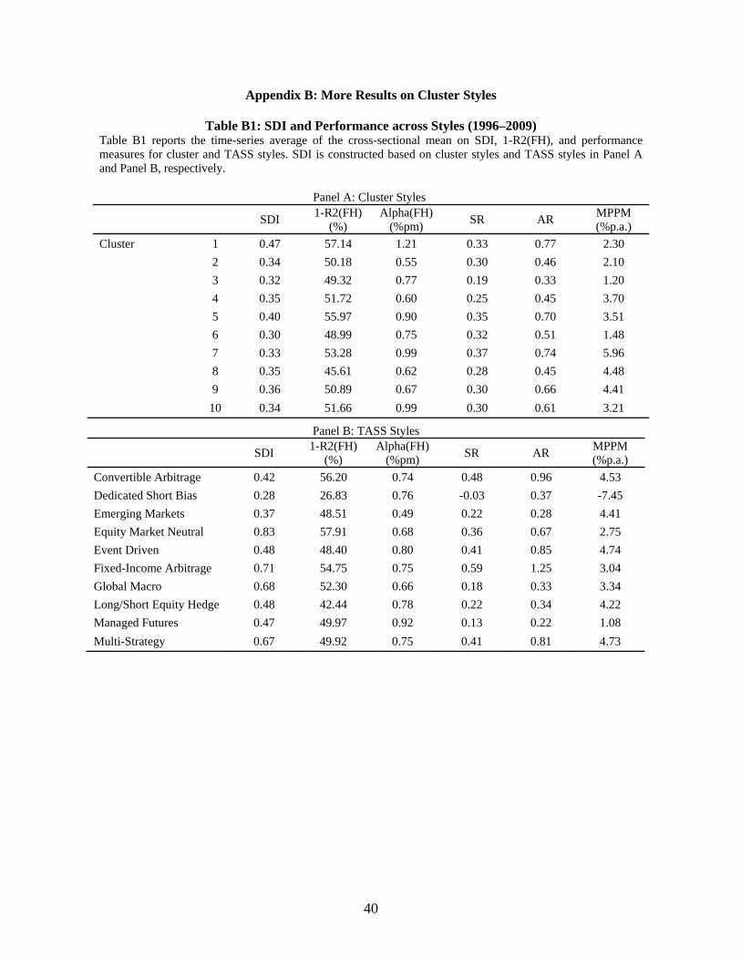
40

Appendix B: More Results on Cluster Styles

Table B1: SDI and Performance across Styles (1996–2009) Table B1 reports the time-series average of the cross-sectional mean on SDI, 1-R2(FH), and performance measures for cluster and TASS styles. SDI is constructed based on cluster styles and TASS styles in Panel A and Panel B, respectively.

Panel A: Cluster Styles

SDI 1-R2(FH)

(%) Alpha(FH)

(%pm) SR AR

MPPM (%p.a.)

Cluster 1 0.47 57.14 1.21 0.33 0.77 2.30

2 0.34 50.18 0.55 0.30 0.46 2.10

3 0.32 49.32 0.77 0.19 0.33 1.20

4 0.35 51.72 0.60 0.25 0.45 3.70

5 0.40 55.97 0.90 0.35 0.70 3.51

6 0.30 48.99 0.75 0.32 0.51 1.48

7 0.33 53.28 0.99 0.37 0.74 5.96

8 0.35 45.61 0.62 0.28 0.45 4.48

9 0.36 50.89 0.67 0.30 0.66 4.41

10 0.34 51.66 0.99 0.30 0.61 3.21

Panel B: TASS Styles

SDI 1-R2(FH)

(%) Alpha(FH)

(%pm) SR AR

MPPM (%p.a.)

Convertible Arbitrage 0.42 56.20 0.74 0.48 0.96 4.53

Dedicated Short Bias 0.28 26.83 0.76 -0.03 0.37 -7.45

Emerging Markets 0.37 48.51 0.49 0.22 0.28 4.41

Equity Market Neutral 0.83 57.91 0.68 0.36 0.67 2.75

Event Driven 0.48 48.40 0.80 0.41 0.85 4.74

Fixed-Income Arbitrage 0.71 54.75 0.75 0.59 1.25 3.04

Global Macro 0.68 52.30 0.66 0.18 0.33 3.34

Long/Short Equity Hedge 0.48 42.44 0.78 0.22 0.34 4.22

Managed Futures 0.47 49.97 0.92 0.13 0.22 1.08

Multi-Strategy 0.67 49.92 0.75 0.41 0.81 4.73

41

Table B2: Cross-Tabulation of Self-Reported TASS Styles and Cluster Styles (200801-200912) Table B2 reports the cross-tabulation of cluster styles with the styles reported by hedge funds in TASS. The TASS styles are those attributed to the funds as of December 2009. The clusters are based on hedge fund returns from January 2008 to December 2009. TASS Style/Cluster Style 1 2 3 4 5 6 7 8 9 10 Row

TotalConvertible Arbitrage 1 1 1 1 16 0 4 20 1 2 47Dedicated Short Bias 0 11 0 0 0 1 0 0 0 0 12Emerging Market 18 10 6 14 67 2 134 39 5 10 305Equity Market Neutral 9 12 9 9 15 2 3 5 30 11 105Event driven 18 11 1 33 85 2 9 17 11 21 208Fixed-Income Arbitrage 2 5 5 3 17 0 2 17 1 6 58Global Macro 19 10 22 7 4 20 16 10 12 4 124Long/Short Equity Hedge 123 26 34 199 106 25 140 54 60 15 782Managed Futures 3 15 20 7 4 137 4 10 12 9 221Multi-Strategy 25 11 9 22 59 11 23 13 17 11 201Column Total 218 112 107 295 373 200 335 185 149 89 2063

42

Table B3: Switching Rate of Pair-Wise Connections between Funds

Table B3 summarizes the pattern of the switching rate of fund clustering results. We study the pair-wise connection between funds based on the cluster groupings obtained at the end of each year; the connection takes the value of 1 or 0, depending on whether the two funds under study fall into the same cluster or not. We then calculate the percentage of pair-wise connections that remain unchanged from year to year. The higher the percentage, the higher the stability of clustering. Column 2 is the sample switching rate, the percentage of connections changed from the previous year clustering results. Column 3 reports the bootstrapped switching rate under the null of random grouping. The null is constructed by forming samples via random draws without replacement from actual fund returns. We follow Abraham, Goetzmann, and Wachter (1994) and Goetzmann and Wachter (1995) for the bootstrap procedure. For each round of the bootstrap procedure, we set the number of clusters and the total number of funds equal to those statistics from the real sample. The last column reports the standard deviation of the bootstrapped null distribution.

Year

Sample Switching Rate Null Switching Rate Std. Dev. of Null Switching Rate

1996 14.63% 29.25% 0.22%

1997 14.74% 29.50% 0.22%

1998 16.78% 29.58% 0.23%

1999 13.86% 29.75% 0.20%

2000 17.90% 29.63% 0.24%

2001 14.04% 29.60% 0.20%

2002 15.79% 29.76% 0.20%

2003 16.77% 29.82% 0.23%

2004 16.22% 29.70% 0.22%

2005 16.99% 29.80% 0.21%

2006 17.32% 29.50% 0.21%

2007 19.86% 29.54% 0.22%

2008 20.25% 29.83% 0.24%

2009 17.20% 29.60% 0.22%

Mean 16.60% 29.63%

43

Appendix C: Heckman Correction - Probit Model

Table C: Hedge Fund Survivorship

Table C presents the probit regression results on hedge funds’ survival probability. The dependent variable is indicator variation that takes a value of one if a fund survives till the end of the next 12 months and zero otherwise. Variable Name Coef. Wald Chi_Squared Pr>ChiSq SDI -0.2743 59.88 <.0001

***

Ln(Age) 0.1233 88.73 <.0001 ***

Ln(AUM) 0.1024 692.10 <.0001 ***

FlowPast1Y 0.0000 0.16 0.6876

VolPast2Y(%p.m) -0.0042 3.54 0.0598 *

AvgPast2YRet 0.1343 536.67 <.0001 ***

AlphaPast2Y 0.0024 4.66 0.0308 **

Time Fixed Effect Yes #FundQtrObs 60621 *** 1% significance; ** 5% significance; * 10% significance

44

References

Abraham, J., Goetzmann, W., and Wachter, S., 1994, Homogeneous Groupings of Metropolitan

Housing Markets, Journal of Housing Economics 3, 186–206. Abreu, D., and Brunnermeier, M., 2002, Synchronization Risk and Delayed Arbitrage, Journal of

Financial Economics 66, 341–360. Ackermann, C., McEnally, R., and Ravenscraft, D., 1999, The Performance of Hedge Funds:

Risk, Return, and Incentives, Journal of Finance 54, 833–874. Agarwal, V., and Naik, N., 2000, Multi-Period Performance Persistence Analysis of Hedge

Funds, Journal of Financial and Quantitative Analysis 35, 327–342. Agarwal, V., and Naik, N., 2004, Risks and Portfolio Decisions Involving Hedge Funds, Review

of Financial Studies 17, 63–98. Agarwal, V., Daniel, N., and Naik, N., 2009, Role of Managerial Incentives and Discretion in

Hedge Fund Performance, Journal of Finance 64 (5), 2221–2256. Aggarwal, R., and Jorion, P., 2009, The Risk of Emerging Hedge Fund Managers, Journal of

Investing 18, 100-107. Aragon, G., 2007, Share Restriction and Asset Pricing: Evidence from the Hedge Fund Industry,

Journal of Financial Economics 83, 33–58. Berk, Jonathan B., and Green, R. C., 2004, Mutual Fund Flows and Performance in Rational

Markets, Journal of Political Economy 112(6), 1269–1295. Brown, S., and Goetzmann, W., 1997, Mutual Fund Styles, Journal of Financial Economics 43,

373–399. Brown, S., and Goetzmann, W., 2003, Hedge Funds with Style, Journal of Portfolio Management

29, 101–112. Brown, S., Goetzmann, W., and Ibbotson, R., 1999, Off-Shore Hedge Funds: Survival and

Performance, Journal of Business 72, 91–117. Brown, S., W. Goetzmann and J. Park, 2001, Careers and Survival: Competition and Risk in the

Hedge Fund and CTA Industry, Journal of Finance 56, 1869–1886. Brown, S., Goetzmann, W., and Ross, S., 1995, Survival, Journal of Finance 50, 853–873. Brown, S., Goetzmann, W., Liang, B., and Schwarz, C., 2008, Mandatory Disclosure and

Operational Risk: Evidence from Hedge Fund Registration, Journal of Finance 63(6), 2785-2815.

Brunnermeier, M., and Nagel, S., 2004, Hedge Funds and the Technology Bubble, Journal of

Finance 59, 2013–2040.

45

Carhart, M., 1997, On Persistence in Mutual Fund Performance, Journal of Finance 52, 57–82. Chen, J., Hong, H., Huang, M., and Kubik, J., 2004, Does Fund Size Erode Mutual Fund

Performance? The Role of Liquidity and Organization, The American Economic Review 90(5), 1276–1302.

Cohen, R., Coval, J. D., and Pástor, L., 2005, Judging Fund Managers by the Company That They

Keep, Journal of Finance 60, 1057–1096. Cremers M., and Petajisto A., 2009, How Active Is Your Fund Manager? A New Measure That

Predicts Performance, Review of Financial Studies 22(9), 3329–3365. Fung, W., and Hsieh, D., 1997, Empirical Characteristics of Dynamic Trading Strategies: The

Case of Hedge Funds, Review of Financial Studies 10, 275–302. Fung, W., and Hsieh, D., 2000, Performance Characteristics of Hedge Funds and CTA Funds:

Natural Versus Spurious Biases, Journal of Financial and Quantitative Analysis 35, 291–307.

Fung, W., and Hsieh, D., 2001, The Risk in Hedge Fund Strategies: Theory and Evidence from

Trend Followers, Review of Financial Studies 14, 313–341. Fung, W., and Hsieh, D., 2002, Benchmarks of Hedge Fund Performance: Information Content

and Measurement Biases, Financial Analysts Journal 58, 22–34. Fung, W., Hsieh, D., Naik, N., and Ramadorai, T., 2008, Hedge Funds: Performance, Risk, and

Capital Formation, Journal of Finance 63, 1777-1803. Gray, W., and Kern, A., 2010, Do Hedge Fund Managers Identify and Share Profitable Ideas?,

University of Chicago Booth School of Business Working Paper. Getmansky, M., Lo, A., and Makarov, I., 2004, An Econometric Model of Serial Correlation and

Illiquidity in Hedge Fund Returns, Journal of Financial Economics 74, 529–609. Goetzmann, W., and Wachter, S., 1995, Clustering Methods for Real Estate Portfolios, Real

Estate Economics 23, 271–310. Goetzmann, W., Ingersoll, J., and Ross, S., 2003, High-Water Marks and Hedge Fund

Management Contracts, Journal of Finance 58, 1685–1717. Griffin, J., and Xu, J., 2009, How Smart Are the Smart Guys? A Unique View from Hedge Fund

Stock Holdings, Review of Financial Studies 22, 2531-2570. Ibbotson, R., and Chen, P., 2006, The A,B,Cs of Hedge Funds: Alphas, Betas, and Costs, Yale

ICF Working Paper No. 06–10. Ingersoll, J., Spiegel, M., Goetzmann, W., and Welch, I., 2007, Portfolio Performance

Manipulation and Manipulation-proof Performance Measures. Review of Financial Studies 20: 1503-46.

46

Jagannathan, R., Malakhov, A., and Novikov, D., 2006, Do Hot Hands Exist Among Hedge Fund Managers? An Empirical Evaluation, NBER Working Paper Series, Vol. w12015.

Kacperczyk, M., and Seru, A., 2007, Fund Manager User of Public Information: New Evidence

on Managerial Skills, Journal of Finance 62, 485–528. Kacperczyk, M., Sialm, C., and Zheng, L., 2005. On the Industry Concentration of Actively

Managed Equity Mutual Funds, Journal of Finance 60, 1983–2011. Kacperczyk, M., Sialm, C., and Zheng, L., 2008. Unobserved Actions of Mutual Funds, Review

of Financial Studies 21 (6), 2379–2416. Kosowski, R., Naik, N. Y., and Teo, M., 2007, Do Hedge Funds Deliver Alpha? A Bayesian and

Bootstrap Analysis, Journal of Financial Economics 84, 229–264. Li, H., Zhang, X., and Zhao, R., 2011, Investing in Talents: Manager Characteristics and Hedge

Fund Performances, Journal of Financial and Quantitative Analysis 46, 59 -82. Liang, B., 1999, On the Performance of Hedge Funds, Financial Analysts Journal 55, 72–85. Liang, B., 2000, Hedge Funds: The Living and the Dead, Journal of Financial and Quantitative

Analysis 35, 309–326. Liang, B., and Park, H., 2008, Share Restriction, Liquidity Premium, and Offshore Hedge Funds,

Working Paper, University of Massachusetts. Lo, A., 2002, The Statistics of Sharpe Ratios, Financial Analysts Journal 58, 36–52. Malkiel, B., and Saha, A., 2005, Hedge Fund: Risk and Return, Financial Analysts Journal 61,

No. 6: 80–88. Petersen, M., 2009, Estimating Standard Errors in Finance Panel Data Sets: Comparing

Approaches, Review of Financial Studies 22, 435-480. Pollet, J., and Wilson, M., 2008, How Does Size Affect Mutual Fund Behavior? Journal of

Finance 63, 2941–2969. Stein, J., 2008, Conversations among Competitors, American Economic Review 98, 2150-2162. Stein, J., 2009, Presidential Address: Sophisticated Investors and Market Efficiency, Journal of

Finance 64, 1517–1548. Titman, S., and Tiu, C., 2011, Do the Best Hedge Funds Hedge? Review of Financial Studies 24

(1), 123–168. Treynor, J., and Black, F., 1973, How to Use Security Analysis to Improve Portfolio Selection,

Journal of Business 46, 66–86. Wahal, S., and Wang, Y., 2011, Competition among Mutual Funds, Journal of Financial

Economics 99, 40–59.

47

Figure 1: Histogram of Hedge Fund SDI

Figure 1A represents the histogram of the SDI based on the cluster styles for all funds for the period 1996–2009. It also depicts a breakdown between the live and graveyard funds in the distribution. Figure 1B represents the histogram of the SDI based on the TASS styles.

0%

5%

10%

15%

20%

25%0.

05

0.15

0.25

0.35

0.45

0.55

0.65

0.75

0.85

0.95

1.05

1.15

1.25

1.35

1.45

1.55

1.65

1.75

1.85

Dis

trib

uti

on

of

Fu

nd

s

Figure 1A: SDI based on Cluster Styles

Graveyard

Live

0%

2%

4%

6%

8%

10%

12%

14%

16%

0.05

0.15

0.25

0.35

0.45

0.55

0.65

0.75

0.85

0.95

1.05

1.15

1.25

1.35

1.45

1.55

1.65

1.75

1.85

Dis

trib

uti

on

of

Fu

nd

s

Figure 1B: SDI based on TASS Styles

Graveyard

Live

48

Figure 2: Histogram of Hedge Fund SDI

Figure 2 represents the relative distribution of funds across the cluster styles for the SDI bins.

0%

10%

20%

30%

40%

50%

60%

70%

80%

90%

100%

0.05 0.15 0.25 0.35 0.45 0.55 0.65 0.75 0.85 0.95

Dis

trib

uti

on

of

Fu

nd

s

Figure 2: SDI Bins

Cluster10

Cluster 9

Cluster 8

Cluster 7

Cluster 6

Cluster 5

Cluster 4

Cluster 3

Cluster 2

Cluster 1

49

Table 1: Summary Statistics (1996–2009) Panel A summarizes the time-series average of cross-sectional summary statistics for the main variables for the full sample, and for the live and graveyard fund subsamples. Variables considered are number of funds per period, the SDI, measured as (1 – correlation) from the clustering program, and contemporaneous fund characteristics including monthly net of fee returns, FH 7-factor adjusted alphas and the corresponding appraisal ratio (AR), Sharpe ratio (SR), manipulation-proof performance measure (MPPM), volatility of monthly net fee returns (Vol), length of redemption notice periods and lockup periods, indicator variables for personal capital commitment and high-water mark, management fees, incentive fees, fund age, AUM, new money flow into funds within the past 12 months as a fraction of AUM, minimum investment, and an indicator variable for using leverage. Panel B reports the time-series average of the pair-wise correlation between these variables.

Panel A: Fund Performance and Characteristics

Full Sample (3,896 unique funds) Live Funds (1,537 unique funds) Graveyard Funds (2,359 unique funds) Mean Median Min Max Std Mean Median Min Max Std Mean Median Min Max Std #Funds per period 1,030 1,075 291 1,657 410 456 336 61 1,234 364 574 638 45 866 228 SDI 0.32 0.29 0.00 0.91 0.18 0.31 0.27 0.00 0.85 0.18 0.32 0.29 0.00 0.88 0.18 NetFeeRet(% p.m.) 0.99 0.74 -25.07 63.76 5.33 1.17 0.86 -17.28 24.61 4.52 0.83 0.63 -21.92 59.72 5.47 Alpha(% p.m.) 0.75 0.68 -5.99 30.34 1.78 0.84 0.75 -3.69 8.29 1.31 0.67 0.62 -5.90 29.07 1.94 AR 0.51 0.38 -1.96 7.50 0.79 0.51 0.40 -1.36 5.44 0.72 0.50 0.37 -1.87 6.94 0.83 SR 0.28 0.22 -1.21 5.42 0.44 0.29 0.25 -0.55 3.26 0.40 0.27 0.20 -1.19 4.90 0.48 MPPM (% p.a.) 3.70 3.86 -89.83 91.41 26.17 5.03 4.79 -80.40 84.55 26.55 2.08 2.55 -86.43 87.85 25.60 Vol(%p.m) 3.99 3.23 0.09 88.79 4.32 4.12 3.41 0.12 24.58 3.06 3.84 3.08 0.13 81.68 4.66 RedemptionNotice (days) 34.35 29.02 0.00 186.61 26.61 35.87 30.00 0.00 186.61 28.20 34.52 28.30 0.00 161.84 26.35 Lockup(months) 3.56 0.00 0.00 58.82 6.38 3.86 0.00 0.00 57.54 6.76 3.55 0.00 0.00 43.73 6.26 PersonalCapDummy 0.46 0.38 0.00 1.00 0.49 0.48 0.48 0.00 1.00 0.49 0.44 0.36 0.00 1.00 0.48 HighWaterMarkDummy 0.56 0.59 0.00 1.00 0.46 0.63 0.96 0.00 1.00 0.47 0.53 0.57 0.00 1.00 0.45 MgmtFee(%) 1.42 1.19 0.00 7.09 0.74 1.50 1.37 0.00 6.79 0.78 1.39 1.17 0.02 5.97 0.70 IncentiveFee(%) 18.17 20.00 0.00 49.40 5.83 19.10 20.00 0.00 35.92 4.32 17.73 20.00 0.00 47.86 6.39 Age(years) 6.63 5.62 2.50 32.07 3.78 6.91 5.88 2.51 25.71 3.90 6.53 5.48 2.50 31.98 3.80 AUM(M$) 192.47 57.88 5.00 7289.08 492.51 194.31 66.90 5.15 4086.93 393.75 211.66 53.14 5.04 7138.99 596.74Flowpast1Y(%p.a.) 16.22 -0.66 -159.09 812.92 80.98 19.95 2.36 -108.47 659.88 77.28 13.77 -1.79 -142.78 745.35 81.28 MinInvestment(M$) 0.98 0.56 0.00 36.61 1.92 1.10 0.54 0.00 33.21 2.26 1.01 0.64 0.00 24.55 1.92 Leverage 0.64 1.00 0.00 1.00 0.48 0.71 1.00 0.00 1.00 0.45 0.61 0.96 0.00 1.00 0.49

(continued)

50

Table 1 – continued

Panel B: Correlations

SDI NetFee

Ret Alpha AR SR MPPM Vol

Redemp-tion

Notice LockupPersonal

Cap

High Water Mark

Mgmt Fee

IncentiveFee Age AUM

Min Invest-ment Leverage

NetFeeRet(% p.m.) 0.01 Alpha(% p.m.) 0.08 0.70 AR 0.18 0.18 0.35 SR 0.17 0.37 0.30 0.82 MPPM (% p.a.) 0.00 0.95 0.50 0.35 0.35 Vol(%p.m) -0.17 0.37 0.28 -0.27 -0.24 0.00 RedemptionNotice 0.04 0.02 0.04 0.20 0.21 0.06 -0.15 Lockup(months) -0.03 0.06 0.06 0.05 0.06 0.04 0.00 0.31 PersonalCap 0.02 0.01 -0.01 -0.03 -0.02 0.01 0.03 0.04 -0.01 HighWaterMark 0.01 0.05 0.05 0.09 0.10 0.04 -0.05 0.25 0.27 -0.08 MgmtFee(%) -0.02 0.06 0.06 -0.05 -0.04 -0.02 0.14 -0.18 -0.12 -0.06 -0.10 IncentiveFee(%) 0.10 0.07 0.07 0.07 0.07 0.01 0.02 0.14 0.10 0.10 0.23 0.04 Age(years) -0.06 -0.02 -0.03 -0.06 -0.06 -0.01 0.02 -0.08 -0.04 0.13 -0.18 0.03 -0.10 AUM(M$) -0.02 0.06 0.03 0.07 0.10 0.00 -0.05 0.08 0.04 0.02 0.01 0.01 -0.03 0.16 Flowpast1Y(%p.a.) 0.04 0.10 0.08 0.06 0.10 0.01 -0.02 0.01 0.01 -0.02 0.05 0.01 0.02 -0.07 0.03 MinInvestment(M$) 0.03 0.01 0.02 0.16 0.14 0.03 -0.12 0.17 0.12 0.04 0.17 -0.05 0.05 0.05 0.21 0.01

Leverage 0.04 0.03 0.02 0.02 0.03 0.00 0.04 -0.04 -0.06 0.15 0.03 0.09 0.18 0.02 0.04 0.01 -0.02

51

Table 2: Persistence of the SDI (1996–2009)

Table 2 reports the time-series means of the average SDI for the current quarter and the subsequent 3 months, 6 months, and 1–3 years for each of the quintile portfolios sorted on the previous 24-month SDI. It also reports the difference between the high and low portfolios and the corresponding t-statistics. In addition, we report the time-series means of number of funds per period at the sorting and at the end of each holding horizon.

Time 0 3m 6m 1y 2y 3y

SDI Low SDI Port 0.10 0.14 0.16 0.19 0.22 0.23

Port2 0.20 0.22 0.23 0.24 0.25 0.26

Port3 0.29 0.30 0.30 0.31 0.31 0.30

Port4 0.40 0.40 0.40 0.39 0.36 0.35

Hi SDI Port 0.60 0.56 0.54 0.50 0.44 0.43

Hi-Lo (SDI) 0.50*** 0.42*** 0.38*** 0.31*** 0.22*** 0.20*** (t-stat) (107.20) (71.42) (48.87) (30.32) (20.87) (24.68)

#Funds 1,025 981 935 850 707 592 *** 1% significance; ** 5% significance; * 10% significance

52

Table 3: Determinants of the SDI (1996–2009)

Table 3 reports the panel regression of the SDI on lagged fund characteristics using annual data:

titiiiti eteristicsFundCharacccSDI ,1,10, Survivorship and backfill biases are controlled for to the

extent the data allow. FH 7-factor alpha and volatility of net fee returns (Vol) are measured over a window of 24 months and are lagged by one year. Other characteristics include lengths of redemption notice periods and lockup periods, indicator variables for personal capital commitment and high-water mark, management fees, incentive fees, fund age, AUM, new money flow into funds, minimum investment, an indicator variable for leverage. Column I includes all funds in the sample. Column II includes only equity related funds, ie. Long/short equity, event driven, dedicated short bias, and equity market neutral. Column III includes only fixed income funds. The coefficients are multiplied by 100. The t-statistics in parentheses are adjusted for fund-clustering effect and time and cluster-style fixed effects.

53

I II III VolPast2Y(%p.m.) -0.58** -1.46*** -1.46** (t-stat) (-2.39) (-6.48) (-2.53)

RedemptionNoticePeriod(30 Days) 0.47 0.15 2.78** (1.34) (0.36) (2.51)

Lockup(months) -0.09** 0.00 0.01 (-2.16) (0.09) (0.07)

PersonalCapitalDummy 0.90 0.68 0.30 (1.64) (1.05) (0.15)

HighWaterMarkDummy -1.11* -1.28* -3.71* (-1.71) (-1.66) (-1.66)

MgmtFee(%) -0.04 2.43*** -2.47 (-0.09) (2.96) (-1.60)

Incentive Fee(%) 0.30*** 0.37*** 0.16 (5.76) (5.47) (0.91)

Age(years) -0.19*** -0.04 0.57* (-3.03) (-0.43) (1.66)

ln(AUM) -0.85*** -1.36*** -0.46 (-4.43) (-6.13) (-0.62)

FlowPast2Y in % 0.01*** 0.00 0.01 (3.19) (1.20) (1.47)

ln(MinInvestment+1) 0.66*** 0.53* -0.56 (3.32) (1.86) (-0.66)

Leverage 1.02* 0.33 1.15 (1.89) (0.52) (0.41)

AlphaPast2Y(%p.m) 1.49*** 1.10*** -0.85 (9.93) (5.02) (-0.89)

Disclosure -1.92** 2.79 (-2.50) (1.05) AdjR2(%) 11.05 15.61 16.75

#FundYearObs. 14,511 8,422 760 *** 1% significance; ** 5% significance; * 10% significance

54

Table 4: Portfolio Performance Based on the SDI (1996–2009) Table 4 reports the time-series means and t-statistics of the post-formation FH 7-factor alphas, FH 7-factor based appraisal ratios (AR), and the smoothing-adjusted Sharpe ratios (SR) for the quintile portfolios sorted on the SDI. The performance measures are based on the equally and value-weighted buy-and-hold portfolios sorted every 3 months and held for 3 months, 6 months, and 1–3 years. The SDI is measured as (1 – correlation), estimated using the clustering procedure. The t-statistics reported below in parentheses are adjusted for heteroscedasticity and autocorrelation.

Panel A: Equally Weighted Portfolios

Alpha (FH 7-factor) Appraisal Ratio Sharpe Ratio (smoothing adjusted)

3m (%p.q.)

6m (%p.sa.)

1y (%p.a)

2y (%p.2y.)

3y (% p.3y.)

3m

6m

1y

2y

3y

3m

6m

1y

2y

3y

LowSDIPort 0.91** 1.80** 3.88*** 8.46*** 12.69*** 0.20*** 0.16*** 0.15*** 0.14*** 0.13*** 0.23*** 0.14** 0.09 0.08** 0.09*** (t-stat) (2.18) (2.33) (3.14) (5.44) (9.95) (2.97) (3.65) (4.25) (5.25) (6.83) (2.80) (2.08) (1.36) (2.27) (3.55)

Port2 1.27*** 2.62*** 5.08*** 10.24*** 16.36*** 0.29*** 0.23*** 0.21*** 0.18*** 0.17*** 0.31*** 0.18*** 0.13** 0.11*** 0.12*** (t-stat) (3.66) (4.29) (4.88) (6.81) (12.44) (4.85) (6.05) (6.90) (7.50) (9.49) (4.35) (3.31) (2.31) (3.18) (4.89)

Port3 1.67*** 3.35*** 6.76*** 13.77*** 18.82*** 0.40*** 0.29*** 0.26*** 0.23*** 0.22*** 0.33*** 0.21*** 0.15*** 0.14*** 0.14*** (tstat) (4.71) (5.13) (5.48) (9.28) (22.10) (7.70) (8.16) (9.40) (10.65) (13.01) (4.94) (3.95) (2.93) (3.96) (5.65)

Port4 1.79*** 3.81*** 6.87*** 14.00*** 20.42*** 0.51*** 0.40*** 0.32*** 0.28*** 0.26*** 0.36*** 0.25*** 0.18*** 0.16*** 0.15*** (t-stat) (5.15) (5.48) (5.81) (10.11) (22.17) (8.28) (8.89) (9.27) (13.38) (21.19) (6.10) (5.44) (4.20) (5.20) (8.55)

HiSDIPort 1.91*** 3.83*** 7.42*** 14.04*** 20.73*** 0.64*** 0.50*** 0.42*** 0.36*** 0.32*** 0.44*** 0.30*** 0.24*** 0.19*** 0.17*** (t-stat) (8.30) (7.84) (7.25) (11.01) (16.40) (9.65) (10.63) (10.97) (15.65) (22.60) (9.76) (10.48) (9.32) (12.05) (14.65)

Hi-Low 1.00*** 2.03*** 3.54*** 5.57*** 8.04*** 0.44*** 0.34*** 0.26*** 0.23*** 0.19*** 0.20*** 0.17*** 0.15*** 0.11*** 0.09*** (t-stat) (2.69) (3.03) (3.26) (4.28) (7.18) (5.29) (5.82) (5.48) (8.03) (9.12) (2.89) (3.48) (3.38) (3.83) (4.12)

Annualized Alpha Hi-Low(%p.a.) 4.05 4.10 3.54 2.75 2.61

(continued)

55

Table 4 – continued

Panel B: Value-Weighted Portfolios

Alpha (FH 7-factor) Appraisal Ratio Sharpe Ratio

3m 6m 1y 2y 3y 3m 6m 1y 2y 3y 3m 6m 1y 2y 3y

LowSDIPort 0.94* 1.63* 3.70** 8.28*** 14.44*** 0.26*** 0.20*** 0.21*** 0.20*** 0.21*** 0.28*** 0.18** 0.13* 0.13*** 0.13*** (t-stat) (1.92) (1.79) (2.44) (4.36) (8.05) (2.77) (3.18) (3.91) (5.18) (6.74) (2.70) (2.40) (1.76) (2.99) (5.01)

Port2 1.44*** 2.70*** 4.27*** 8.72*** 15.27*** 0.41*** 0.32*** 0.26*** 0.24*** 0.24*** 0.42*** 0.26*** 0.17** 0.16*** 0.17*** (t-stat) (3.39) (3.26) (2.91) (3.46) (4.93) (4.84) (5.91) (5.89) (5.89) (6.33) (4.80) (3.61) (2.53) (3.32) (5.15)

Port3 1.60*** 3.38*** 7.18*** 14.62*** 21.38*** 0.50*** 0.37*** 0.32*** 0.29*** 0.28*** 0.37*** 0.25*** 0.20*** 0.19*** 0.17*** (t-stat) (3.03) (3.76) (4.28) (5.49) (9.54) (6.54) (6.83) (7.23) (7.83) (8.29) (3.22) (3.65) (3.14) (4.07) (4.74)

Port4 1.69*** 3.55*** 5.25*** 11.71*** 18.19*** 0.61*** 0.46*** 0.36*** 0.33*** 0.32*** 0.38*** 0.29*** 0.21*** 0.19*** 0.20*** (t-stat) (3.30) (3.54) (2.66) (4.03) (7.87) (8.40) (8.40) (6.42) (7.50) (9.91) (4.79) (5.21) (3.67) (4.07) (5.20)

HiSDIPort 1.48*** 2.80*** 6.24*** 12.92*** 19.13*** 0.83*** 0.67*** 0.57*** 0.51*** 0.43*** 0.54*** 0.38*** 0.29*** 0.23*** 0.21*** (t-stat) (2.64) (3.14) (4.87) (9.20) (11.70) (8.16) (8.01) (7.70) (10.82) (16.97) (7.45) (6.16) (5.21) (6.74) (8.57)

Hi-Low 0.54 1.16 2.53* 4.64*** 4.69*** 0.58*** 0.47*** 0.36*** 0.31*** 0.23*** 0.26** 0.20*** 0.16*** 0.10** 0.08*** (t-stat) (0.99) (1.24) (1.75) (3.17) (2.85) (4.80) (4.90) (4.42) (6.08) (6.28) (2.28) (2.71) (2.74) (2.56) (2.63)

Annualized Alpha Hi-Low(%p.a.) 2.18 2.34 2.53 2.29 1.54 *** 1% significance; ** 5% significance; * 10% significance

56

Table 5 Manipulation-Proof Performance for SDI Portfolios (1996–2009)

Table 5 reports the time-series means of the post-formation manipulation-proof performance measure (MPPM), for the quintile portfolios sorted on the SDI. The performance measures are based on the equally and value-weighted buy-and-hold portfolios sorted every 3 months and held for 3 months, 6 months, and 1–3 years. The SDI is measured as (1 – correlation), estimated using the clustering procedure. The p-values for the high-low portfolio results are based on a bootstrap procedure described in the text.

Equally Weighted Portfolios (% p.a.) Value-Weighted Portfolios (% p.a.)

3m 6m 1y 2y 3y 3m 6m 1y 2y 3y

LowSDIPort 2.74 1.19 -0.79 -1.68 -1.47 2.63 1.28 -0.09 -0.89 -0.25

Port2 3.72 2.52 0.73 -0.62 -0.32 4.67 3.16 1.31 -0.26 0.05

Port3 3.73 2.94 1.33 0.02 -0.22 4.09 3.57 2.20 0.62 -0.21

Port4 3.86 3.19 1.27 0.11 0.11 2.60 2.48 -0.55 -0.96 -0.95

HiSDIPort 3.39 2.68 1.83 0.42 0.26 3.09 2.10 1.32 0.42 0.37

Hi-Low 0.66* 1.49*** 2.62*** 2.11*** 1.73*** 0.47 0.82 1.41* 1.31** 0.62

bootstrapped p-value (0.05) (<0.01) (<0.01) (<0.01) (<0.01) (0.35) (0.24) (0.06) (0.03) (0.15)

57

Table 6: Panel Regression of Hedge Fund Performance on the SDI (1996–2009)

Table 6 reports the panel regression results for hedge fund performance on SDI at the quarterly frequency

as follows: titiitiiiti eControlcSDIccrformanceAbnormalPe ,1,21,10, . Survivorship and

backfill biases are controlled for to the extent the data allow. Alpha is the FH 7-factor adjusted performance over the subsequent 1 year in percentage terms. AR, SR, and MPPM are the corresponding appraisal ratio, smoothing-adjusted Sharpe ratio, and manipulation-proof performance measure, respectively. Control variables are the lagged fund characteristics, including volatility of monthly net fee returns (Vol), length of redemption notice periods and lockup periods, indicator variables for personal capital commitment and high-water mark, management fees, incentive fees, fund age, AUM, new money flow into funds within the preceding 12 months as a fraction of AUM, in percent, minimum investment, and an indicator variable for using leverage. The t-statistics reported in parentheses are adjusted for fund-clustering effect and time and cluster style fixed effects. Panel Regression alpha(% p.a.) AR SR MPPM FH 7-factor FH 7-factor (% p.a.) SDI 3.35*** 0.34*** 0.27*** 3.54*** (t-stat) (3.02) (6.86) (6.56) (4.41)

VolPast2Y(%p.m) 0.13 -0.32*** (0.85) (-3.80)

RedemptionNotice(30Days) 0.55** 0.08*** 0.05*** 0.71*** (2.12) (3.76) (3.84) (3.54)

Lockup(months) 0.08** 0.00* 0.00 0.02 (2.37) (-1.75) (-1.60) (0.86)

PersonalCapitalDummy -0.32 -0.04** -0.01 0.62* (-0.79) (-1.99) (-0.56) (1.88)

HighWaterMarkDummy 1.22** 0.01 0.02 1.62*** (2.40) (0.59) (0.99) (4.20)

MgmtFee(%) 0.78** -0.01 0.01 1.01*** (2.28) (-0.82) (0.75) (4.18)

IncentiveFee(%) 0.04 0.00 0.00 0.05 (0.80) (-1.25) (-0.97) (1.51)

Age(years) -0.01 0.00 0.00 0.13*** (-0.27) (1.52) (1.31) (3.40)

ln(AUM) -0.57*** 0.02*** 0.01*** -0.39*** (-4.23) (4.61) (3.36) (-3.36)

FlowPast1Y(%) 0.00* 0.00 0.00 0.00 (-1.79) (0.73) (1.15) (1.24)

AvgPast2YRet(% p.m.) 0.08 -0.01*** 0.02*** 0.33* (0.28) (-3.12) (4.27) (1.73)

ln(MinInvestment+1) 0.68*** 0.03*** 0.02*** 0.57*** (4.84) (5.08) (5.43) (4.04)

Leverage 0.25 0.02 0.03* 0.30 (0.59) (0.92) (1.80) (0.88)

AdjR2(%) 5.39 8.86 14.82 19.26 #FundQtrObs. 53,071 53,071 47,643 52,311 *** 1% significance; ** 5% significance; * 10% significance

58

Table 7: Fama-MacBeth Analysis of Hedge Fund Performance on the SDI (1996–2009)

Table 7 reports the Fama-MacBeth regression results for hedge fund performance on the SDI and other fund characteristics at the quarterly frequency as the following:

titiitiiiti eControlcSDIccrformanceAbnormalPe ,1,21,10, . Survivorship and backfill

biases are controlled for to the extent the data allow. Alpha is the FH 7-factor adjusted performance over the subsequent 1 year in percentage terms. AR, SR, and MPPM are the corresponding appraisal ratio, smoothing-adjusted Sharpe ratio, and manipulation-proof performance measure, respectively. Control variables are the lagged fund characteristics, including volatility of monthly net fee returns volatility, length of redemption periods and lockup periods, indicator variables for personal capital commitment and high-water mark, management fees, incentive fees, fund age, AUM, new money flow into funds within the preceding 12 months as a fraction of AUM, in percentage, minimum investment, and an indicator variable for using leverage. Cluster-style dummies are included in the regressor set. The t-statistics (reported below the estimated coefficients in italicized font) are adjusted for heteroscedasticity and autocorrelation. Fama-MacBeth Regression alpha(% p.a.) AR SR MPPM FH 7-factor FH 7-factor (% p.a.) SDI 3.82** 0.38*** 0.22*** 3.00* (t-stat) (2.51) (5.27) (5.02) (1.78)

VolPast2Y(%p.m) 0.07 -0.45** (0.30) (-2.01)

RedemptionNotice(30Days) 0.58** 0.08*** 0.05*** 0.60** (2.20) (6.34) (5.09) (2.53)

Lockup(months) 0.14*** 0.00* 0.00 0.05 (2.63) (-1.78) (-1.38) (1.09)

PersonalCapitalDummy -0.33 -0.03*** -0.02 0.12 (-0.71) (-3.69) (-1.62) (0.33)

HighWaterMarkDummy 0.96 0.03 0.02 1.43*** (1.13) (1.44) (1.58) (2.89)

MgmtFee(%) 1.03** -0.01 0.01* 1.25*** (2.42) (-0.89) (1.73) (3.88)

IncentiveFee(%) 0.01 0.00 0.00 0.02 (0.32) (-1.50) (-1.64) (0.57)

Age(years) -0.05 0.00 0.00 0.04 (-0.82) (0.74) (0.19) (0.76)

ln(AUM) -0.57** 0.03*** 0.01*** -0.35** (-2.43) (3.83) (2.99) (-1.96)

FlowPast1Y(%) 0.00 0.00** 0.00 0.00 (-1.35) (2.33) (0.91) (-0.38)

AvgPast2YRet(% p.m.) 0.50 -0.02 0.02** 1.16* (0.74) (-1.04) (2.50) (1.95)

ln(MinInvestment+1) 0.76*** 0.03*** 0.02*** 0.47*** (3.42) (5.19) (7.83) (3.27)

Leverage 0.50 0.02 0.03** 0.33 (1.22) (1.33) (2.41) (0.82)

AdjR2(%) 17.59 15.84 13.57 21.59 *** 1% significance; ** 5% significance; * 10% significance

59

Table 8: Robustness: Hedging Effect (1996-2009)

Panel A of Table 8 reports the summary statistics of the percentage of funds in the SDI-sorted quintile portfolios that fall into the same quintile sorted according to 1-R2(FH). Panel B reports the time-series means of the post-formation FH 7-factor alphas, FH 7-factor based appraisal ratios (AR), the smoothing-adjusted Sharpe ratios (SR), and the manipulation-proof performance measure (MPPM), for the SDI-sorted quintile portfolio using funds that do not fall into the same quintile when sorted on 1-R2(FH). The performance measures are based on the equally and value-weighted buy-and-hold portfolios sorted every 3 months and held for 1 year. We report below in parentheses t-statistics for alpha, AR, and SR, and bootstrapped p-value for MPPM. The t-statistics are adjusted for heteroscedasticity and autocorrelation. Panel C reports the panel regression and Fama-MacBeth regression results for hedge fund performance on SDIs, 1-R2(FH) and other fund characteristics at the quarterly frequency as the following:

titiitiitiiiti eControlcFHRcSDIccrformanceAbnormalPe ,1,31,21,10, ))7(21( . Control variables

are the lagged fund characteristics, including volatility of monthly net fee returns (Vol), length of redemption notice periods and lockup periods, indicator variables for personal capital commitment and high-water mark, management fees, incentive fees, fund age, AUM, new money flow into funds within the preceding 12 months as a fraction of AUM, in percentage, minimum investment, and an indicator variable for using leverage. Panel regression is adjusted for fund-clustering effect and time and style fixed effects, and Fama-MacBeth regression controls for style dummies and adjusts for heteroscedasticity and autocorrelation in standard errors. For brevity, only the estimation results for the SDI and 1-R2(FH) are reported here. Survivorship and backfill biases are controlled for to the extent the data allow.

60

Panel A: Ratio of Overlapped Funds in Quintile Portfolios Sorted by SDI and by 1-R2(FH 7-factor)

Low SDI Port 2 Port 3 Port 4 Hi SDI

Mean 0.50 0.31 0.27 0.30 0.48

Median 0.51 0.32 0.27 0.29 0.47

Min 0.34 0.16 0.19 0.20 0.29

Max 0.64 0.43 0.36 0.41 0.62 Std 0.07 0.05 0.04 0.05 0.07

Panel B: Returns on Quintile Portfolios Sorted by SDI While Excluding Funds in the Same Rank Sorted by 1-R2(FH 7-factor)

EW

alpha(% p.a.)

FH 7-factor AR

(FH) SR

VW

alpha(% p.a.)

FH 7-factorAR

(FH) SR

MPPM(% p.a.)

MPPM (% p.a.)

Low SDI Port 3.71* 0.17*** 0.08 -1.30

Low SDI Port 3.04 0.21*** 0.13* -0.69

(1.72) (3.31) (1.38) (1.12) (2.86) (1.89)

Port 2 5.32*** 0.21*** 0.13** 0.52 Port 2 4.42*** 0.26*** 0.17*** 1.17

(4.65) (7.07) (2.47) (3.25) (6.71) (2.65)

Port 3 6.77*** 0.26*** 0.15*** 1.21 Port 3 7.31*** 0.34*** 0.20*** 2.23

(5.39) (9.57) (2.92) (4.56) (7.04) (3.14)

Port 4 6.71*** 0.31*** 0.18*** 1.18 Port 4 5.02** 0.35*** 0.21*** -0.41

(6.31) (9.34) (4.13) (2.46) (6.86) (3.69)

Hi SDI Port 7.40*** 0.36*** 0.20*** 1.84 Hi SDI Port 6.02*** 0.48*** 0.24*** 1.57

(7.95) (10.56) (9.16) (3.94) (7.63) (5.13)

Hi-Lo 3.69** 0.19*** 0.12** 3.13*** Hi-Lo 2.98 0.27*** 0.11* 2.26**

(1.97) (2.97) (2.43) (<0.01) (1.17) (2.70) (1.65) (0.03)

Panel C: Regression Analysis (Other control variables in Table 6 are included in the regression but not reported below for brevity.)

Panel Regression Fama-MacBeth

alpha(% p.a.) FH 7-factor

AR FH 7-factor SR

MPPM (% p.a.)

alpha(% p.a.)FH 7-factor

AR FH 7-factor SR

MPPM (% p.a.)

SDI 2.10* 0.18*** 0.23*** 4.25*** 1.07 0.29*** 0.21*** 3.21 (tstat) (1.78) (4.24) (5.62) (4.93) (0.48) (3.34) (4.07) (1.48)

1-R2(FH 7-factor) 2.22** 0.27*** 0.08*** -1.27 4.45 0.16*** 0.01 -0.22 (tstat) (2.13) (7.49) (2.59) (-1.58) (1.52) (2.77) (0.26) (-0.11)

*** 1% significance; ** 5% significance; * 10% significance

61

Table 9: Robustness: Survivorship Bias (1996–2009) Table 9 Panel A reports the time-series means of the survival rate, in percentage, for quintile portfolios sorted on the SDI. The portfolios are sorted every 3 months and held for 3 months, 6 months, and 1–3 years. It also reports the difference between the high and low portfolios, and the corresponding t-statistics. Panel B reports the regression analysis with Heckman adjustment. The control variables for the regression are the same as the regression reported in Table 6 and 7. Panel A: Portfolio Sorting

3m 6m 1y 2y 3y SDI Low SDI Port 95.41 90.75 81.55 67.93 55.32 Port2 95.28 90.57 82.03 67.68 55.86 Port3 95.06 90.18 80.99 66.23 54.52 Port4 94.94 89.73 80.28 65.09 53.00 Hi SDI Port 94.40 88.82 78.76 63.63 51.41

Hi-Lo (SDI) -1.01** -1.93*** -2.79** -4.30*** -3.91*** (tstat) (-2.36) (-2.80) (-2.22) (-4.04) (-2.95)

Panel B: Regression Analysis with Heckman Adjustment (Other control variables in Table 6 are included in the regression but not reported for brevity.)

Panel Regression Fama-MacBeth

alpha(% p.a.) FH 7-factor

AR FH 7-factor SR

MPPM (% p.a.)

alpha(% p.a.)FH 7-factor

AR FH 7-factor SR

MPPM (% p.a.)

SDI 3.31*** 0.34*** 0.27*** 3.73*** 3.67** 0.38*** 0.21*** 2.87* (t-stat) (3.01) (6.92) (6.64) (4.66) (2.38) (5.36) (4.95) (1.69)

Heckman Lambda 4.13*** 0.10*** 0.10*** 4.21*** 4.31*** 0.11*** 0.10*** 4.26*** (t-stat) (18.36) (10.43) (10.49) (16.06) (10.16) (8.96) (8.20) (6.35) AdjR2(%) 6.65 9.60 15.81 20.59 18.80 16.92 15.44 23.70 #FundsQtrObs. 52,947 52,947 47,531 52,189

*** 1% significance, ** 5% significance, * 10% significance

62

Table 10: Robustness: Absolute Correlation-Based SDI (1996-2009)

Panel A of Table 10 reports the summary statistics of the percentage of funds in the SDI-sorted quintile portfolios that also fall into the same quintile sorted according to corrSDI . Panel B reports the time-

series means of the post-formation FH 7-factor alphas, FH 7-factor based appraisal ratios (AR), the smoothing-adjusted Sharpe ratios (SR), and the manipulation-proof performance measure (MPPM), for the

corrSDI -sorted quintile portfolio. The performance measures are based on the equally and value-

weighted buy-and-hold portfolios sorted every 3 months and held for 1 year. We report below in parentheses t-statistics for alpha, AR, and SR, and bootstrapped p-value for MPPM. The t-statistics are adjusted for heteroscedasticity and autocorrelation. Panel C reports the panel regression and Fama-MacBeth regression results for hedge fund performance on corrSDI and other fund characteristics at the

quarterly frequency as the following: titiitiiiti eControlccorrSDIccrformanceAbnormalPe ,1,21,10, . Alpha is the compounded FH 7-

factor adjusted performance over the subsequent 1 year in percentage terms. AR and SR are the corresponding appraisal ratio and smoothing-adjusted Sharpe ratio. Control variables are the lagged fund characteristics including volatility of monthly net fee returns (Vol), length of redemption notice periods and lockup periods, indicator variables for personal capital commitment and high-water mark, management fees, incentive fees, fund age, AUM, new money flow into funds within the preceding 12 months as a fraction of AUM, in percentage, minimum investment, and an indicator variable for using leverage. Panel regression is adjusted for fund-clustering effect and time- and style-fixed effects, and Fama-MacBeth regression controls for style dummies and adjusts for heteroscedasticity and autocorrelation in standard errors. For brevity, only the estimation results for the SDIs are reported here. Survivorship and backfill biases are controlled for to the extent the data allow.

63

Panel A: Ratio of Overlapped Funds in Quintile Portfolios Sorted by SDI(Corr)- and SDI(|corr|) Low SDI Port 2 Port 3 Port 4 Hi SDI

Mean 0.79 0.63 0.63 0.66 0.82

Median 0.78 0.60 0.59 0.64 0.81

Min 0.66 0.50 0.46 0.44 0.63

Max 1.00 1.00 1.00 1.00 1.00 Std 0.07 0.11 0.12 0.11 0.06

Panel B: Returns of Quintile Portfolios Sorted on SDI(|corr|)

EW

alpha(% p.a.)

FH 7-factor AR

(FH) SR

VW

alpha(% p.a.)

FH 7-factorAR

(FH) SR

MPPM(% p.a.)

MPPM (% p.a.)

Low SDI Port 3.53*** 0.15*** 0.09 -0.84

Low SDI Port 3.67** 0.21*** 0.13* 0.17

(2.61) (3.70) (1.36) (2.39) (3.89) (1.76)

Port 2 5.70*** 0.21*** 0.13** 0.95 Port 2 5.70*** 0.28*** 0.17** 2.14

(5.42) (7.47) (2.31) (3.72) (6.96) (2.53)

Port 3 6.37*** 0.25*** 0.15*** 1.01 Port 3 6.47*** 0.30*** 0.20*** 1.12

(5.65) (8.53) (2.93) (3.73) (6.26) (3.14)

Port 4 7.38*** 0.33*** 0.18*** 1.75 Port 4 5.59*** 0.39*** 0.21*** -0.07

(5.81) (10.77) (4.20) (2.78) (6.58) (3.67)

Hi SDI Port 7.03*** 0.41*** 0.24*** 1.50 Hi SDI Port 6.09*** 0.57*** 0.29*** 1.45

(7.14) (10.67) (9.32) (4.82) (8.62) (5.21)

Hi-Lo 3.50*** 0.26*** 0.15*** 2.34*** Hi-Lo 2.41* 0.36*** 0.16*** 1.28*

(2.77) (5.09) (3.38) (<0.01) (1.75) (4.76) (2.74) (0.08)

Panel C: Regression Analysis (Other control variables in Table 6 are included in the regression but not reported below for brevity.)

Panel Regression Fama-MacBeth

alpha(% p.a.) FH 7-factor

AR (FH) SR

MPPM (% p.a.)

alpha(% p.a.)FH 7-factor

AR (FH) SR

MPPM(% p.a.)

SDI(|Corr|) 4.50*** 0.38*** 0.23*** 3.18*** 4.04** 0.34*** 0.15*** 2.19 (tstat) (3.61) (7.07) (5.79) (3.53) (2.17) (3.99) (3.44) (1.16)

AdjR2(%) 5.06 8.69 14.92 18.99 17.11 16.54 15.23 21.02#FundsQtrObs 53,071 53,071 47,643 52,311

*** 1% significance; ** 5% significance; * 10% significance

64

Table 11: Robustness: TASS Style-based SDI (1996–2009)

Panel A of Table 11 reports the summary statistics of the percentage of funds in the SDI-sorted quintile portfolios that also fall into the same quintile sorted according to SDI(TASS). Panel B reports the time-series means of the post-formation FH 7-factor alphas, FH 7-factor based appraisal ratios (AR), the smoothing-adjusted Sharpe ratios (SR), and the manipulation-proof performance measure (MPPM), for the SDI(TASS)--sorted quintile portfolio. The performance measures are based on the equally and value-weighted buy-and-hold portfolios sorted every 3 months and held for 1 year. We report below in parentheses t-statistics for alpha, AR and SR, and bootstrapped p-value for MPPM. The t-statistics are adjusted for heteroscedasticity and autocorrelation. Panel C reports the panel regression and Fama-MacBeth regression results for hedge fund performance on SDI(TASS) and other fund characteristics at the quarterly frequency as the following:

titiitiiiti eControlcTASSSDIccrformanceAbnormalPe ,1,21,10, . We report results for both the raw

and standardized SDI, which is the difference between the raw SDI and the average SDI of the corresponding style scaled by the cross-sectional standard deviation of SDI within the same style. Alpha is the compounded FH 7-factor adjusted performance over the subsequent 1 year in percentage terms. AR and SR are the corresponding appraisal ratio and smoothing-adjusted Sharpe ratio. Control variables are the lagged fund characteristics including volatility of monthly net fee returns (Vol), length of redemption notice periods and lockup periods, indicator variables for personal capital commitment and high-water mark, management fees, incentive fees, fund age, AUM, new money flow into funds within the preceding 12 months as a fraction of AUM, in percentage, minimum investment, and an indicator variable for using leverage. Panel regression is adjusted for fund-clustering effect and time- and style-fixed effects, and Fama-MacBeth regression controls for style dummies and adjusts for heteroscedasticity and autocorrelation in standard errors. For brevity, only the estimation results for the SDIs are reported here. Survivorship and backfill biases are controlled for to the extent the data allow.

65

Panel A: Ratio of Overlapped Funds in Quintile Portfolios Sorted by SDI and by SDI(TASS) Low SDI Port 2 Port 3 Port 4 Hi SDI

Mean 0.57 0.36 0.32 0.35 0.55

Median 0.58 0.36 0.32 0.35 0.54

Min 0.34 0.21 0.19 0.19 0.37

Max 0.72 0.48 0.45 0.50 0.74 Std 0.09 0.07 0.07 0.07 0.10 Panel B: Portfolio Sorting Results

EW

alpha(% p.a.)

FH 7-factor

AR (FH) SR

VW

alpha(% p.a.)

FH 7-factorAR

(FH) SR

MPPM(% p.a.)

MPPM (% p.a.)

Low SDI Port 3.85*** 0.18*** 0.10 -0.75 Low SDI Port 3.34 0.24*** 0.16** 0.08

(2.67) (4.37) (1.55) (1.51) (3.93) (2.01)

Port 2 5.94*** 0.23*** 0.14** 1.32 Port 2 9.10*** 0.35*** 0.20*** 2.93

(5.99) (7.80) (2.52) (4.19) (7.36) (2.94)

Port 3 6.50*** 0.26*** 0.15*** 1.35 Port 3 6.45*** 0.33*** 0.19*** 0.26

(5.64) (9.82) (2.75) (4.25) (7.36) (2.85)

Port 4 6.59*** 0.33*** 0.18*** 1.24 Port 4 6.44*** 0.44*** 0.21*** 0.87

(5.43) (10.99) (4.11) (4.38) (7.55) (3.58)

Hi SDI Port 7.12*** 0.36*** 0.21*** 1.21 Hi SDI Port 2.73 0.38*** 0.22*** -0.22

(6.60) (8.54) (10.20) (1.62) (5.87) (5.99)

Hi-Lo 3.27** 0.18*** 0.11** 1.96*** Hi-Lo -0.61 0.13** 0.06 -0.30

(2.14) (3.76) (2.41) (<0.01) (-0.40) (2.42) (1.04) (0.63)

Panel C: Regression Analysis (Other control variables in Table 6 are included in the regression but not reported below for brevity.)

Panel Fama-MacBeth

alpha(% p.a.) FH 7-factor

AR (FH) SR

MPPM (% p.a.)

alpha(% p.a.)FH 7-factor

AR (FH) SR

MPPM(% p.a.)

Reg 1 SDI(TASS) 2.27*** 0.05*** 0.07*** 2.57*** 3.23** 0.07 0.02 0.17 (t-stat) (3.45) (3.16) (4.91) (5.22) (2.08) (1.54) (0.40) (0.09) Reg 2 SDI(Cluster) 3.35*** 0.34*** 0.27*** 3.54*** 3.82** 0.38*** 0.22*** 3.00* (t-stat) (3.02) (6.86) (6.56) (4.41) (2.51) (5.27) (5.02) (1.78) *** 1% significance; ** 5% significance; * 10% significance

66

Table 12: Robustness: Alternative Backfill Bias Control (1997–2009)

Table 12 summaries the results, where the backfill bias is controlled by filtering out data prior to a fund entering the TASS database. Panel A reports the time-series means of the post-formation FH 7-factor alphas, FH 7-factor based appraisal ratios (AR), the smoothing-adjusted Sharpe ratios (SR), and the manipulation-proof performance measure (MPPM), for the SDI-sorted quintile portfolio. The performance measures are based on the equally and value-weighted buy-and-hold portfolios sorted every 3 months and held for 1 year. We report below in parentheses t-statistics for alpha, AR and SR, and bootstrapped p-value for MPPM. The t-statistics are adjusted for heteroscedasticity and autocorrelation. Panel B reports the panel regression and Fama-MacBeth regression results for hedge fund performance on SDI and other fund characteristics at the quarterly frequency as the following:

titiitiiiti eControlcSDIccrformanceAbnormalPe ,1,21,10, . Alpha is the compounded FH 7-

factor adjusted performance over the subsequent 1 year in percentage terms. AR and SR are the corresponding appraisal ratio and smoothing-adjusted Sharpe ratio. Control variables are the lagged fund characteristics including volatility of monthly net fee returns (Vol), length of redemption notice periods and lockup periods, indicator variables for personal capital commitment and high-water mark, management fees, incentive fees, fund age, AUM, new money flow into funds within the preceding 12 months as a fraction of AUM, in percentage, minimum investment, and an indicator variable for using leverage. Panel regression is adjusted for fund-clustering effect and time- and style-fixed effects, and Fama-MacBeth regression controls for style dummies and adjusts for heteroscedasticity and autocorrelation in standard errors. For brevity, only the estimation results for the SDIs are reported here.

67

Panel A: Returns of Quintile Portfolios Sorted on SDI

EW

alpha(% p.a.)

FH 7-factor AR

(FH) SR

VW

alpha(% p.a.)

FH 7-factorAR

(FH) SR

MPPM(% p.a.)

MPPM (% p.a.)

Low SDI Port 1.70 0.12*** 0.06 -4.01 Low SDI Port 1.66 0.20*** 0.12 -2.81

(0.91) (2.82) (0.95) (0.65) (2.90) (1.62)

Port 2 3.29** 0.18*** 0.10* -1.73 Port 2 2.48 0.24*** 0.13 -0.77

(2.01) (4.55) (1.67) (0.95) (3.99) (1.62)

Port 3 4.44*** 0.23*** 0.11** -1.14 Port 3 2.85 0.28*** 0.18*** -0.35

(3.14) (6.62) (2.22) (1.14) (4.33) (2.83)

Port 4 6.10*** 0.29*** 0.16*** 0.46 Port 4 2.13 0.35*** 0.24*** -0.76

(4.50) (9.29) (3.86) (0.98) (6.16) (3.80)

Hi SDI Port 6.58*** 0.37*** 0.22*** 0.91 Hi SDI Port 4.59*** 0.52*** 0.28*** 0.43

(5.06) (10.52) (8.41) (2.96) (6.97) (5.39)

Hi-Lo 4.88*** 0.25*** 0.16*** 4.92*** Hi-Lo 2.93 0.33*** 0.16** 3.25***

(3.16) (5.56) (3.33) (<0.01) (1.17) (4.37) (2.52) (<0.01)

Panel B: Regression Analysis Other control variables in Table 6 are included in the regression but not reported below for brevity.

Panel Regression Fama-MacBeth

alpha(% p.a.) FH 7-factor

AR (FH) SR

MPPM (% p.a.)

alpha(% p.a.)FH 7-factor

AR (FH) SR

MPPM (% p.a.)

SDI 5.71*** 0.38*** 0.31*** 5.49*** 6.95*** 0.41*** 0.29*** 7.55*** (t-stat) (4.63) (7.94) (7.10) (5.83) (3.66) (5.61) (4.12) (3.47)

AdjR2(%) 5.93 8.59 14.00 19.92 15.70 15.88 15.20 21.34 #FundsQtrObs 41,415 41,415 32,916 40,239

*** 1% significance; ** 5% significance; * 10% significance