* We thank Daron Acemoglu, Joshua Angrist, Lawrence Katz, David Lee, Emmanuel Saez and participants at the NBER Labor Studies spring 2009 meeting for valuable suggestions. We also thank David Lee for providing data on minimum wage laws by state. Autor acknowledges financial support from the National Science Foundation (CAREER SES‐0239538). 

The Role of the Minimum Wage in the Evolution of U.S. Wage Inequality  over Three Decades: A Modest Re‐Assessment* 

David Autor MIT Department of Economics and NBER 

Alan Manning London School of Economics 

Christopher L. Smith Federal Reserve Board of Governors 

 May 2009 

PRELIMINARY 

We offer a fresh analysis of the effect of state and federal minimum wages on earnings inequality over 1979 to 2007, exploiting substantially longer state‐level wage panels than were available to earlier studies as well as a proliferation of recent state minimum wage laws. We obtain identification using cross‐state and over‐time variation in the ‘bite’ of federal and applicable state minimum wages, as per influential studies by Lee (1999) and Teulings (2000, 2003). We address two econometric issues that may afflict earlier work: simultaneity bias stemming from both errors‐in‐variables and from a non‐zero correlation between mean state wages and latent state wage variances.  We find, consistent with prior work, that the minimum wage reduces inequality in the lower tail of the wage distribution. But the estimated effects, corrected for both sources of bias, are considerably smaller than suggested by earlier OLS estimates: the minimum wage explains at most 50% of the rapid rise in female inequality during the 1980s, 25% of the rise in male inequality, and 30 – 40% of the rise in pooled gender inequality. Though modest, these impacts are still larger than would be implied if the minimum wage only raised wages at or below the statutory minimum, suggesting the presence of spillovers from the minimum to higher percentiles. We estimate these spillovers by structurally fitting the latent wage distribution, calculating the mechanical effect of the minimum wage through truncation, and inferring spillovers by comparison of the mechanical and observed distributions. Spillovers appear to account for a substantial amount of the minimum’s modest impact on percentiles in the lower tail of the wage distribution. Subsequent analysis shows, however, that spillovers and measurement error have similar implications for the effect of the minimum wage on the shape of the measured wage distribution at the lower tail. With available precision, we cannot reject the hypothesis that the full effect of the minimum wage on the actual wage distribution is due exclusively to direct effects of the statutory minimum wage on the percentiles where it binds rather than spillovers to higher percentiles. Accepting this null, the implied effect of the minimum wage on the actual wage distribution is smaller than the effect of the minimum wage on the measured wage distribution.  

   

1 

 

Introduction

While economists have vigorously debated the effect of the minimum wage on employment 

levels for at least six decades (cf. Stigler, 1946), its contribution to the evolution of earnings 

inequality—that is, the shape of the earnings distribution—was largely overlooked prior to the 

seminal 1996 contribution of DiNardo, Fortin and Lemieux (DFL hereafter). Using kernel density 

techniques, DFL produced overwhelming visual evidence that the minimum wage substantially 

‘held up’ the lower tail of the US earnings distribution in 1979, yielding a pronounced spike in 

hourly earnings at the nominal minimum value, particularly for females. By 1988, however, this 

spike had virtually disappeared. Simultaneously, the inequality of hourly earnings increased 

markedly in both the upper and lower halves of the wage distribution. Most relevant to this 

paper, the female 10/50 (‘lower tail’) log hourly earnings ratio expanded by 23 log points (two 

thirds) between 1979 and 1988, while male and pooled‐gender 10/50 ratios grew by 5.7 and 

10.5 log points in the same interval (Table 1). To assess the causes of this rise, DFL constructed 

counterfactual wage distributions that potentially account for the impact of changing worker 

characteristics, labor demand, union penetration, and minimum wages on the shape of the 

wage distribution. Comparing counterfactual with observed wage densities, DFL conclude that 

the erosion of the federal minimum wage—which declined in real terms by 30 log points 

between 1979 and 1988—was the predominant cause of rising lower tail inequality between 

1979 and 1988, explaining two‐thirds of the growth of the 10/50 for both males and females.1  

Though striking, a well‐understood limitation of the DFL findings is that the counterfactual 

wage distributions derive exclusively from reweighting of observed wage densities rather than 

controlled comparisons. As such, the DFL exercise is closer in spirit to simulation than inference. 

Cognizant of this limitation, DFL highlight in their conclusion that the expansion of lower tail 

inequality during 1979 to 1988 was noticeably more pronounced in ‘low‐wage’ than ‘high‐wage 

states,’ consistent with the hypothesis that the falling federal minimum caused a differential 

increase in lower tail equality in states where the minimum wage was initially more binding. 

                                                       

1 DFL attribute 62 percent of the growth of the female 10/50 and 65 percent of the growth of the male 10/50 to the declining value of the minimum wage (Table III). 

2 

 

Building on this observation, Lee (1999) exploited cross‐state variation in the gap between state 

median wages and the applicable federal or state minimum wage (the ‘effective minimum’) to 

estimate what the share of the observed rise wage inequality during 1979 through 1991 was 

due to the falling minimum rather than changes in underlying (‘latent’) wage inequality. 

Amplifying the conclusions of DFL, Lee estimated that more than the entire rise of lower tail 

earnings inequality between 1979 and 1989 was due to the falling federal minimum wage; had 

the minimum been constant throughout this period, observed wage inequality would have 

fallen.2  

These influential findings present a number of puzzles. First, the rise in lower tail inequality 

during the 1980s was accompanied by an equally pronounced increase in dispersion in the 

upper‐half (90/50) of the distribution (Figure 1B), an area where the minimum is unlikely to be 

relevant. Though the contemporaneous rises in upper and lower tail inequality need not have 

identical causes, it would be surprising if they had no causes in common. Second, at no time 

between 1979 and 2007 were more than six percent of male hours paid at or below the federal 

(or applicable state) minimum wage (Table 1). If the falling minimum wage explains the bulk of 

the rise in male wage lower‐tail inequality, this implies extremely large spillovers from the 

minimum wage to non‐covered workers. Finally, the Lee analysis uncovers, and scrupulously 

reports, a number of puzzling results that cast some doubt on the validity of the exercise. Most 

surprisingly, the main estimates imply that the declining federal minimum wage substantially 

reduced the growth of upper‐tail inequality in both the male and pooled‐gender wage 

distributions during 1979 to 1991, a finding that appears implausible on a priori grounds.3  

Spurred by these puzzles, we offer a fresh analysis of the impact of state and federal 

minimum wages on the shape of the US earnings distribution. Our work benefits from 

substantially longer state‐level wage panels than were available to earlier studies, and from a 

                                                       

2 Using cross‐region rather than cross‐state variation in the ‘bindingness’ of minimum wages, Teulings (2000 and 2003) reaches similar conclusions. See also Mishel, Bernstein and Allegretto (2006, chapter 3) for an assessment of the minimum wage’s effect on wage inequality.  3 See Lee (1999) Table II. The large, positive and highly significant coefficients in this table imply that a 1 log point in the effective minimum wage (defined as the difference between the log state minimum wage and the log state median wage), reduces male and pooled‐gender 90/50 log wage inequality by 0.16 to 0.44 log points.  

3 

 

proliferation of state minimum wage laws enacted after 2000 that generate usable state 

variation in wage floors.4 Our statistical approach follows closely the model of Lee and Teulings; 

we obtain identification by using cross‐state and over‐time variation in the ‘bindingness’ of 

federal and applicable state minimum wages. The main advance of our approach is in 

estimation. Because the impact of the minimum wage will in part depend upon where in the 

wage distribution the statutory minimum falls, it is necessary to scale the statutory minimum by 

some measure of expected ‘bindingness.’ Lee (1999) proposes a natural scaling: the gap 

between the log state minimum and log state median wage, which Lee labels the ‘effective 

minimum.’  

This approach introduces two potential confounds. The first arises if state median wages 

levels are correlated with the latent variance (i.e., absent the minimum wage) of state wage 

distributions, i.e., if states with high median wages have relatively high (or low) underlying 

wage variances.5 In this case, the use of the state median to calculate the ‘effective minimum 

wage’ measure will bias estimates of the effect of the minimum on wage inequality upward or 

downward, depending on the nature of the mean‐variance correlation. The second, more 

mundane, concern with using the median to calculate the effect minimum is that the median 

wage appears on both sides of the estimating equation, i.e., in the effective minimum wage and 

in the 10/50 earnings ratio and other inequality metrics. This is problematic inasmuch as 

sampling variation in the median wage may generate simultaneity bias in OLS models that leads 

to inflated estimates of the effect of the minimum on state wage distributions.6   

We find that both of these confounds are empirically important. In particular, median state 

log wages and log wage variances are strongly positively correlated, even in portions of the 

distribution where the variance of wages is unlikely to be affected by the minimum wage (such 

as the log(60)‐log(40) gap). This pattern indicates that states with high median wages have 

                                                       

4 As of 2007, 30 states had established state minimum wages that exceeded the federal level (Table 1). 5 Lee (1999) is explicit on this point: The estimation assumes that the scale (variance) of state wage distributions is independent of state medians conditional on year effects.  6 Cognizant of the possibility of simultaneity bias, Lee takes a number of steps to minimize its impact. These steps do not appear to fully resolve the problem, as we show below.  

4 

 

relatively high and persistent levels of latent wage inequality, necessitating inclusion of state 

fixed effects (and in some cases trends) in our primary models. State effects exacerbate the 

problem of simultaneity bias resulting from errors‐invariables, however. The reason is that 

more of the remaining variation in the effective minimum wage is the result of sampling 

variation.  

To purge this simultaneity bias, we apply the canonical (Durbin, 1954) technique of 

instrumenting the error‐ridden measure with a set of variables that do not share common 

measurement error with the error‐ridden variable. Our first instrumental variables strategy is to 

instrument the effective minimum wage (statutory minimum minus state median) with the 

statutory minimum wage in each state and year. This follows an approach first used by Card, 

Katz and Krueger (1993) in their reanalysis of the employment effects of minimum wage laws. A 

second approach is to employ split‐sample instrumental variables (‘SSIV,’ cf. Angrist and 

Krueger, 1995). We use half of the estimation sample (chosen at random) to compute the 

effective minimum and wage percentiles, while using the other half to form a second estimate 

of the effective minimum wage that serves as an instrumental variable for the first.  For 

purposes of comparison to these IV estimates, we also replicate the OLS models used in Lee 

(1999) and extend them to 2007. 

Our main results are as follows. In partial confirmation of prior work, we find that the 

minimum wage significantly affects the shape of the US wage distribution during the 1980s, 

particularly for females. However, OLS estimates substantially overestimate the contribution of 

the minimum wage to inequality due to violation of the identification assumptions discussed 

above. The bias is most severe for the male and pooled‐gender wage distributions, but is also 

pronounced for the female distribution.7 During the period of 1979 through 1988, when the 

erosion of the minimum wage was most rapid, OLS estimates suggest that latent wage 

inequality was mostly unchanged during 1979 to 1988 or increased modestly. By contrast, 2SLS 

models indicate that the minimum wage explains less than half of the substantial increase in 

                                                       

7 The problem is likely more severe for the male and the pooled distributions because the minimum wage is largely non‐binding in these samples. Hence, the significant minimum wage coefficient in OLS models appears primarily due to a combination of the two identification issues outlined above.  

5 

 

female inequality during this period, about one quarter of the increase for males, and about 

40% of the increase for the pooled gender distribution. Graphical comparisons of OLS and 2SLS 

estimates reinforce the conclusion that OLS estimates are unlikely to be reliable. 

To benchmark the applicability of these findings outside of the closely studied period of 

1979 through 1988, we also calculate the contribution of the minimum wage to inequality 

during 1998 to 2007. During this time, the employment‐weighted average of state minimum 

wages fell by 10.6 log points. 2SLS estimates indicate that the falling minimum contributed 

modestly to male, female, and pooled‐gender wage inequality during both periods. By contrast, 

OLS models generally suggest that the declining minimum either masked compressions of 

(latent) inequality or that latent growth in inequality was not as great as suggested by 2SLS 

estimates—a result that likely derives from simultaneity bias.  

The modest effects of the minimum on inequality that we identify may arise through two 

channels: a direct (mechanical) impact whereby wages below the minimum are increased;8 and 

an indirect (spillover) effect whereby earnings above the minimum are also pushed upward 

(due perhaps to incentive or equity considerations). While our 2SLS models capture the net of 

these two effects, it is also of interest to analyze their separate contributions since any usable 

forecast of the effect of the minimum on wage inequality must account for spillovers (if 

present).  

Identifying these spillovers requires an empirical model of the full latent distribution of 

wages (or at least its lower tail), purged of both direct and indirect minimum wage effects. We 

model each state’s latent wage distribution as log‐normal. We estimate the parameters of 

these distributions using wage observations from higher percentiles of the distribution, where 

the minimum wage is unlikely to be relevant. We then calculate the mechanical impact of the 

minimum wage by truncating the lower tail of the (estimated) latent distribution, and we infer 

spillovers by comparing the ‘mechanical’ distribution with the observed distribution.  

                                                       

8 We assume no disemployment effects at the modest minimum wage levels mandated in the US, an assumption that is supported by a large recent literature.  

6 

 

Though the minimum wage had only a modest effect on inequality over 1979 to 2007, 

spillovers were a significant component of this impact. At its highest level (in 1979), the 

minimum wage mechanically raised the 10th percentiles of the female distribution by 20 log 

points, and spillovers raised percentiles by an additional 2 log points. Both the direct and 

spillover effects were considerably smaller for males and for the pooled distribution. As the real 

minimum eroded between 1979 and 2007, the direct impact of the minimum wage on 

observed 50/10 inequality fell substantially, so that by the mid‐2000s, the majority of the 

observed minimum wage effect on the 50/10 was due to spillovers of the minimum wage onto 

percentiles above where it bound.  

A drawback of these spillover estimates is that they may be in part be driven by 

measurement error in wage reporting rather true wage spillovers. In particular, if a subset of 

workers that are paid the minimum wage tends to report wage values that are modestly above 

or below the true minimum—and if the central tendency of this reporting error moves in 

tandem with the minimum wage—this may create the appearance of spillovers where none are 

present. Thus, despite the apparent existence of substantial spillovers in the measured wage 

distribution, it’s possible that the spillovers to the actual wage distribution are smaller or non‐

existent.  

To explore this possibility, we perform a bounding exercise that compares the estimated 

effect of the minimum wage on mean wages (which should not be biased by measurement 

error) with the magnitude of the spike in the wage distribution at the statutory minimum, 

corrected for measurement error.  Under the null hypothesis that the minimum wage has direct 

effects but no spillovers, we show that the elasticity of the mean log wage with respect to the 

log minimum is equal to the size of this spike. For most years, the estimated mean effect 

remains within the upper and lower bounds of the estimated spike.  Based on this analysis, we 

are unable to reject the hypothesis that all of the apparent effect of the minimum wage on 

percentiles above the minimum is the consequence of measurement error. Accepting this null, 

the implied effects of the minimum wage on the actual wage distribution are even smaller than 

the effects of the minimum wage on the measured wage distribution. 

7 

 

The remainder of the paper proceeds as follows. Section I describes the data and presents 

simple, reduced‐form estimates of the relationship between the statutory minimum wage and 

inequality throughout the distribution. Section II presents more fully parameterized models 

that, like Lee (1999), explicitly account for the bite of the minimum wage in estimating its effect 

on the wage distribution. This section compares parameterized OLS and 2SLS models, and 

documents the pitfalls that arise in the OLS estimation. Section III summarizes our 

counterfactual exercise in which, following Lee, we use point estimates from the main 

regression models to calculate counterfactual changes in wage inequality holding the real 

minimum wage constant. Section IV presents estimates of the magnitude of spillovers from the 

minimum wage onto percentiles above where it directly binds, derived from parametric 

estimates of the latent wage distribution that provide a full accounting of mechanical and 

spillover effects. Section V describes results from an exercise explores the potential 

contribution of measurement error to the identification of spillover effects.  The final section 

concludes. 

I. Change in the federal minimum wage and variation in state minimum wages

The Federal minimum wage remained constant in nominal terms over the nine‐year period 

between 1981 and 1990. Similarly, the Federal minimum wage remained at $5.15 between 

September 1997 and July 2007, and by July 2007, the real value of the Federal minimum was 

lower than it had been at any point in the past fifty years (Figure 1). The difference between the 

two periods is that by the late 1980s, only 15 states minimum wages exceeded the federal 

minimum wage; by 2007, 30 state minimum wages did. As a result, the average real value of 

the minimum wage applicable to workers in 2007 was not much lower than it was in 1997, and 

was significantly higher than if states had not enacted their own minimum wages. Appendix 

Table 1 illustrates the extent of state minimum wage variation between 1979 and 2007. 

We use these differences in minimum wages across states and over time as one source of 

variation for identifying the impact of the minimum wage on the wage distribution. As an 

additional form of variation, we use the notion that the wage distribution of lower wage states 

8 

 

should be more affected for a given value of the real minimum wage. Table 1 provides 

examples of this. For each year, there is significant variation in the percentile of the state wage 

distribution where the state or federal minimum wage “binds.” For instance, in 1979 the 

minimum wage was equal to the 3rd percentile of the female wage distribution in Nevada, equal 

to the 31st percentile in Mississippi, and the median percentile at which it bound, across all 

states, was around the 12th percentile. In 1979, this variation in the “bite” or “bindingness” of 

the minimum wage is due mainly to cross‐state differences in wage levels, since only Alaska had 

a state minimum wage that exceeded the federal minimum. In later years—particularly 2000 

and after—this variation is also due to differences in the value of state minimum wages. 

A. Sample and variable construction 

Our analysis uses the percentiles of states’ annual wage distributions as the primary 

outcomes of interest. We form these by pooling all individual responses from the Current 

Population Survey Merged Outgoing Rotation Group (CPS MORG) for each year. An individual’s 

wage is taken to be his reported hourly wage, if the individual reports being paid by the hour, 

and is otherwise calculated as weekly earnings divided by weekly hours worked. We limit the 

sample to individuals age 18 through 64, and we multiply top‐coded values by 1.5. We exclude 

self‐employed individuals and those with wages imputed by the BLS. We make no adjustment 

for individuals with particularly low wages (i.e. sub‐minimum wages). We then take these 

individual wage data and calculate all percentiles of the male, female, and pooled state wage 

distributions for 1979‐2007, weighting individual observations by their CPS sampling weight 

multiplied by their weekly hours worked.  

Our primary analysis is at the state‐year level. However, minimum wages often change 

during the middle of a year. We resolve this by assigning the value of the minimum wage that 

was in effect the longest throughout the calendar year to the state‐year observation. For those 

states and years in which a different minimum wage was in effect for six months in the year, 

the maximum of the two is used. Alternatively, we have tried assigning the maximum of the 

minimum wage within a year as the applicable minimum wage, and this leaves our conclusions 

unchanged.  

9 

 

II. Parametric estimation of minimum wage effects on the wage distribution

A. Econometric framework 

To properly make inference about the impact of the minimum wage at all percentiles of the 

wage distribution, we are interested in estimating specifications for which the impact of the 

minimum wage is a function of not only the real value of the minimum wage, but is also a 

function of the overall shape or location of the wage distribution. One way to do this is to scale 

the minimum wage by some measure of the general level of wages.  Lee (1999) estimated 

minimum wage effects in this spirit, and used the log of the minimum relative to the median as 

his measure of the ‘bite’ of the minimum wage. We will also use this measure and refer to it as 

the effective minimum. 

Use of the effective minimum can be justified in the following way, which fleshes out the 

arguments used by Lee (1999).  Denote by   the log wage in state s at time t for percentile 

p in the absence of the minimum wage—call this the latent wage distribution.  With a minimum 

wage, denoted in log form by  , the actual log wage at percentile p, which we will denote by 

( )stw p  will deviate from the latent distribution for at least some percentiles.  If, for example, 

the minimum wage had no effect on employment rates, and no spillovers then we would have 

the relationship: 

  ,   (1)

However, if there are spillovers or some employment effects, then the minimum wage will 

have an effect on percentiles above where it binds (see Lee, 1999, for more discussion of these 

arguments, or Teulings, 2000, for an explicit supply and demand model with this feature).  So, 

let us generalize (1) to the form: 

  ,   (2)

What are plausible restrictions on the function  . , . ?  We would expect it to be increasing 

in both its arguments and that it also satisfies a homogeneity property—that if the latent 

10 

 

percentile and the minimum wages both rise in the same proportion, the actual percentile also 

rises in that proportion.  As the model is expressed in logs this restriction can be written as: 

  , ,   (3)

Now set   and applying (3) to (2) we have that:  

  0,   (4)

i.e., the deviation of the actual percentile from the latent percentile depends on the gap 

between the minimum and the latent percentile.  What are the plausible restrictions on the 

function  . ?  We would expect it to be positive everywhere (otherwise the minimum wage 

would reduce wages at some percentiles) and to have a positive first derivative.  In addition, if 

the minimum wage is very low (or non‐existent) we would expect the actual percentile to be 

very close to the latent percentile so that we have  ∞ 0.  On the other hand, if the 

minimum wage gets very high we would expect the actual percentile to be very close to the 

minimum wage so that we have lim .  Graphically, we might expect that the 

relationship between deviations of the actual from the latent percentile and the difference 

between the minimum wage and the latent percentile looks something like that presented in 

Figure 2. In this figure, the x‐axis plots the difference between the minimum and the latent 

value of percentile p. The y‐axis plots the difference between the observed and latent values of 

percentile p. For low values of the minimum wage relative to the latent percentile, the 

minimum wage has no effect on the wage distribution so the observed value of the percentile is 

the latent value. For percentiles for which the minimum wage exceeds the latent percentile, the 

observed percentile will be equal to the minimum wage.  

Figure 2 also allows for the possibility of ‘spillovers’ where the minimum either raises wages 

that are latently below the minimum to a value exceeding the minimum, or raises wages that 

are latently above the minimum to a value exceeding their latent level. If present, such 

spillovers would be largest at the location where the minimum wage exactly equals the latent 

11 

 

wage value (in Figure 2, this is the intersection of the x and y axes).9 Spillovers would be 

expected to attenuate in either direction from this point: further down the wage distribution, 

the minimum becomes extremely binding and so the mechanical effect dominates; further 

upward, the minimum wage becomes increasingly less relevant.  

This discussion should make it clear that non‐linearity is likely to be an important feature of  

(4) so that some thought needs to be given to the functional form of the estimating equation.  

In what follows, our main specification uses a quadratic approximation (as does Lee, 1999), and 

we approximate (4) by:  

     

 

(5)

However, it should be noted that a quadratic cannot have a shape similar to that drawn in 

Figure 2 over the whole of its range so that we have to exercise caution in estimating minimum 

wage effects outside the observed sample.  In particular, this specification cannot be used for 

an assessment of what the distribution of wages would be like if there was no minimum wage. 

To make (5) into an estimable equation wage we need to put some additional structure on 

the form taken by the latent wage distribution.  We follow Lee (1999) in assuming that the 

latent wage distribution can be summarized by 2 parameters – the median and the variance – 

so that we can write: 

    (6)

We have the normalization  50 0 so that   is the median log wage in state s at 

time t.  Plugging (6) into (5) and collecting terms we have that:    

  12   (7)

The first two terms are related to the overall evolution of wage inequality and last two terms to 

the effect of the effective minimum.  Note that the coefficients in (7) will vary with the 

                                                       

9 Any effect of the minimum at this location is a pure spillover since the minimum wage is non‐binding at . 

12 

 

percentile, not just because p appears in the linear term of the effective minimum but also 

because, as pointed out by White (1980), the coefficients   will vary with the data.  Intuitively 

we would expect that a rise in latent wage inequality leads to a larger impact on lower 

percentiles for a given effective minimum.  

For (7) to be estimable one also needs models for the median and variance.  There are a 

number of potential options, and we start our discussion with the choices made by Lee.  Lee 

replaces   by the observed median,   by a set of time dummies and assumes that any cross‐

state variation in latent wage inequality is uncorrelated with the median and can therefore be 

subsumed into the error without causing bias in the estimated impact of the minimum wage.  

Hence, equation (7) can be written as:  

  50 50 50   (8)

 In columns (1), (6), and (11) of Table 2 we present estimates of the marginal effects of the 

effective minimum when estimated at the weighted average of the effective minimum over all 

states and all years between 1979‐2007 for selected percentiles.  If we look at the lower 

percentiles, we find, as Lee did, large significant effects of the minimum wage extending 

throughout all percentiles below the median for the male, female and pooled wage 

distributions.  Additionally, we estimate modest effects of the minimum wage at the top of the 

male and pooled wage distributions. Figures 3A, 4A, and 5A plot the estimated marginal effects 

of the minimum wage at each percentile. Taking these results at face value would seemingly 

suggest that the minimum wage affects the entirety of the wage distribution, and implies a 

systematic relationship between the effective minimum wage and upper wage percentiles of 

the male and pooled distributions. 

One possible form of misspecification is that the identifying assumption that state latent 

wage inequality is uncorrelated with the median is false. Indeed if we regress the log(60)‐log 

(40) on the median (which should be uncorrelated if the density function is symmetric around 

the median) and time dummies (to capture the controls put in equation (8)), the log median has 

a t‐statistic of 16 for females, 3.7 for men and 13.6 for the combined sample.  This suggests that 

those states with high median wages have high levels of latent wage inequality.  Since this 

13 

 

seemingly indicates permanent differences in latent wage inequality across states, state fixed 

effects should be included in estimation of (8). Lee also reports this type of specification (Tables 

II and III), and we display estimates from OLS estimation of (8) with state fixed effects in 

columns (2), (7), and (12) of Table 2. Columns (3), (8), and (13) add state‐specific time trends, 

and the marginal effects as implied by these estimates are plotted in Figures 3B, 4B, and 5B. 

The inclusion of state fixed effects or state‐specific time trends yields a large and positive 

relationship between the effective minimum wage and upper tail percentiles for all samples. 

The last two columns in panels A, B, and C estimate first‐differenced analogues to equation (8). 

Estimated marginal effects remain similar to what is observed when estimating the equation in 

levels. 

The explanation for this problem is almost certainly a point made by Lee (1999)—the 

presence of the median in both the dependent and independent variables in (8) induces an 

artificial positive correlation caused by sampling variation. This potentially gets worse when 

state fixed effects are included, as more of the remaining variation is the result of sampling 

variation. 

Lee (1999) is aware of this problem and, as a potential solution, uses two different 

measures of central tendency in the dependent and independent variables:  the median in the 

dependent variable, but trimmed mean on the right‐hand side (i.e. the mean after excluding 

the bottom and top 30 percentiles).  Although this does reduce the correlation, it does not 

eliminate it. In fact, one can show that if the latent log wage distribution is normal, the 

correlation between the trimmed mean and the median will be about 0.93—i.e. not one, but 

very high (see the derivation in the Appendix).  So, this method does not necessarily solve the 

problem. 

Here, we use another method to estimate the relationship represented by (8).  Instead of 

estimating with OLS, we instrument the effective minimum terms.  We use two distinct sets of 

instruments.  For the first set, we use the legislated minimum wage (the maximum of the 

federal minimum wage and the state’s minimum wage) and its square, and the minimum wage 

interacted with a measure of the average wage in the state between 1979 and 2007 (we use 

the average of each state’s median).  This latter instrument is to give us instruments which 

14 

 

differ in their ability to discriminate between the linear and quadratic terms10. Since legislated 

minimum wages provide identification using changes to state minimum wage laws, the 

instrument identifies minimum wage effects for the wage distribution of states which increase 

their minimum wages above the federal minimum. A shortcoming of this instrument is that 

there is quite limited cross‐state variation in the legislated minimum wage during the 1980s. 

This makes identification based on the legislated minimum wage instrument tenuous in this 

period.   

As an alternative instrument, which provides broad identification for all states and all years, 

we use a variant on split sample instrumental variables (Angrist and Krueger 1995).  In 

particular, we split the sample in two halves (choosing observations at random).  We use the 

first half to calculate wage percentiles and the effective minima by state and by year.  We use 

the second half to produce a second estimate of the effective minima (again, by state and by 

year), which then serve as instrumental variables for the first set. We repeat this procedure 50 

times (each time drawing a new random division of the data), and average the resulting 

coefficients. The bottom two rows of Table 3 provide F‐statistics from testing the joint 

significance of the five instruments—the legislated minimum wage and the legislated minimum 

squared, the interaction term, and the effective minimum and its square as estimated in the 

other half of the sample.  Jointly, the instruments are highly significant across all specifications. 

Columns (1), (6), and (11) of Table 3 present estimates of the marginal effect of the 

effective minimum wage from equation (8) with 2SLS. The estimated impact of the minimum 

wage is large and significant throughout the lower half of the female, male, and pooled wage 

distributions. Adding state fixed effects reduces the magnitude of minimum wage effects 

everywhere throughout the distribution, though also results in a significant positive relationship 

between the effective minimum wage and upper tail inequality in all samples. This correlation 

                                                       

10 More precisely, the instruments for equation (8) are  ,  ,  · 50 ,  50 , and  50 , where  50  is the average median within a state between 1979 and 2007, and the last two 

expressions are the effective minimum and its square as estimated from the second half of the sample. The instruments for the first‐differenced analogue, which we describe more fully below, are ∆ , ∆ ,   50 ·∆ , ∆ 50 , and ∆ 50 2, where ∆  represents the annual change in the log of the legislated minimum wage. 

15 

 

with upper tail inequality suggests that shocks to the wage distribution may be correlated with 

changes in minimum wages. Consistent with this, the addition of state‐specific time trends 

(columns (3), (8), and (13)) somewhat breaks the association between the effective minimum 

and upper‐tail percentiles.11 Figures 3C, 4C, and 5C provide a clearer picture of how the 

minimum wage is estimated to affect inequality throughout the wage distribution using this 

specification. After including state trends, the association between the effective minimum wage 

and upper‐tail inequality is much more modest, and minimum wage effects are significant 

through the 30th percentile of the wage distribution for each of the three samples. The 

magnitude of the effects is largest at the bottom of the female wage distribution, and smallest 

at the bottom of the male wage distribution, which is as expected given the overall higher male 

wage levels. 

In addition to estimating equation (8) in levels with state fixed effects, we also estimate the 

equation in its first‐differenced form. Columns (4), (9), and (14) provide estimates of the first‐

differenced analogue to the levels specification with state fixed effects, and columns (5), (10), 

(15) include state fixed effects as well (and is therefore analogous to the inclusion of state 

trends in the levels estimation). Figures 4D, 5D, and 6D plot the marginal effects across all wage 

percentiles for this last set of estimates. The estimated impact of the minimum wage is 

somewhat smaller in magnitude throughout the lower tail of the distribution than when the 

causal effects are estimated in levels. In addition, the effects are less precisely estimated12. 

To summarize, our estimates imply that a 10 log point increase in a state’s effective 

minimum reduces female 50/10 inequality by between 1.3‐2.7 log points, male inequality by 

about 1 log point, and pooled gender inequality by 1.5‐2 log points. OLS estimates are at least 

2.5 times as large as 2SLS estimates (and typically greater), and imply a substantial impact of 

the minimum wage on inequality throughout most of the wage distribution.  

                                                       

11 Recent work on the employment effects of the minimum wage have argued for the inclusion of state trends for this reason. See, for instance, Allegretto, Dube, and Reich (2008). 12 As robustness checks, we have also estimated models with a cubic in the effective minimum, and estimated using monthly or quarterly data rather than yearly data, and found similar results (results available upon request). 

16 

 

III. Benchmarking the effect of the minimum wage on the shape of the wage distribution

Our analysis confirms a significant impact of the minimum wage on wage inequality. To 

develop a precise sense of the size of this contribution, we conduct two sets of analyses. The 

first, following Lee (1999), uses point estimates from the main models to estimate the changes 

in wage inequality that would counterfactually have occurred had the minimum wage held 

constant at a given real level. This analysis provides an estimate of the net contribution of the 

minimum to wage inequality. It does not distinguish between mechanical and spillover effects, 

however. The second analysis decomposes these two effects through a more ambitious 

modeling exercise. 

A. Counterfactual wage inequality estimates with the real minimum held constant 

A straightforward approach to gauging the contribution of the minimum wage to inequality 

trends is to use the earlier regression estimates to calculate counterfactual wage distributions, 

holding the effective minimum wage constant.  Following Lee (1999), we calculate for each 

observation in the dataset its rank in its respective state‐year wage distribution. We then adjust 

each wage by the quantity:  

  ∆ , , , ,   (9)

where  ,  is the observed end‐of period effective minimum in state s in some year 1,  ,  

is the corresponding beginning‐of‐period effective minimum in 0, and  ,  are point 

estimates from the OLS and 2SLS estimates in Tables 2 and 3. We pool these adjusted wage 

observations to form a counterfactual national wage distribution, and we compare changes in 

inequality in the simulated distribution to those in the observed distribution. 13 One feature of 

this simulation procedure bears note: it does not permit estimation of the full ‘latent’ 

distribution of wages—i.e., in the absence of any minimum wage—since the effective minimum 

                                                       

13 Also distinct from Lee, we use states’ observed median wages when calculating   rather than the national median deflated by the price index. This choice has no substantive effect on the results, but appears most consistent with the identifying assumptions.  

17 

 

wage measure, equal to the logarithm of the minimum minus the logarithm of the median, is 

undefined at a minimum wage of zero. This simulation tool is therefore appropriate for 

estimating the impact of the minimum wage over ranges observed in the data. We address this 

infirmity in the subsequent sub‐section.  

 Panel A of Table 4 shows that the female 50/10 log wage ratio increased by 23.4 log points 

between 1979 and 1988. To form counterfactual estimates of what the 50/10 would have been 

in 1979 had the minimum wage been at its lower 1988 value throughout, we adjust 1979 wages 

by the procedure outlined above. Applying the OLS point estimates from Table 2 (column 1 ) to 

this exercise, we calculate that the 50/10 would counterfactually have risen by approximately 

3.2 log points over this period had the state 1979 effective minimums actually been at 1988 

levels, using coefficients obtained by estimating equation (8) over the full 1979 to 2007 sample 

(column 1) or 1979 to 1988 (column 2). Thus, consistent with Lee (1999), OLS estimates imply 

that the minimum wage can account for the bulk (20.2 of 23.4 log point increase, or 85%) of the 

observed expansion of lower tail female wage inequality in this period.14  

The next four rows of the table present analogous counterfactuals estimated using 2SLS in 

lieu of OLS. We present four sets of counterfactuals. The first two counterfactuals are based 

upon 2SLS estimates of equation (8), including state and year fixed effects and state‐specific 

time trends (that is, estimates from columns 3, 8, and 13 of Table 3). The second set are based 

on first‐differenced 2SLS estimates of (8), including state and year fixed effects (columns 5, 10, 

and 15 of Table 3).  For each set of estimates, we use two different instrument sets. The first 

uses split‐sample IV only. The second also includes the log of the legislated minimum wage, its 

square, and its interaction with the average median wage for a state.  

Using coefficients estimated for  the full sample duration (column 1), the 2SLS first‐

differenced estimates imply that the falling minimum wage explains no more than 7.6 of the 23 

log point expansion of the female lower tail (33%) during 1979 through 1998. Fixed effect 

                                                       

14 Lee (1999, Table IV) estimates that the female 50/10 rose by 18.6 log points between 1979 and 1989, and that the falling minimum accounts for all but 4.5 log points of this increase. We focus on the interval of 1979 to 1988 rather than 1979 to 1989 because wage lower tail wage inequality for males had already begun to reverse course by 1989. If we instead focus on 1979 to 1989, our results are substantively identical. 

18 

 

estimates imply a somewhat larger contribution, however, (around 16 or 17 log points, or 

about 50%). Using estimated coefficients from models estimated only over 1979 to 1988 

(column 2), the estimated contribution of the minimum wage is similar to that from the full 

sample when the instrument set includes only split‐sample instruments.  When including state 

minimum wages as additional instruments, the minimum is estimated to have a large impact, 

with contributions approaching those from OLS models. Since at most 10 states have minimum 

wages that exceed the federal minimum during this period, the identifying variation from using 

state minimum wages is stronger for these states than for others.  For this reason, we view the 

inclusion of state minima in the instrument set as inappropriate when using the shortened 1979 

to 1988 sample.   

For the most part, these counterfactual estimates represent significant downward revisions 

in the contribution of the minimum wage to rising female inequality over the 1980s from what 

is implied by OLS estimates. When these calculations are repeated for the male and pooled‐

gender wage distributions (panels B and C), the contrast between OLS and 2SLS estimates is at 

least as sharp. OLS models imply that male and pooled‐gender lower‐tail inequality would have 

contracted in the absence of a falling minimum wage. 2SLS estimates instead suggest that the 

minimum explains no more than one‐fifth of the total expansion of the male 50/10, and no 

more than 40% of the rise in the 50/10 for the pooled distribution.   

How robust are these findings across time periods and specifications? In columns (4), (5), 

and (6) of Table 4, we calculate identical regression‐based counterfactuals for 1998 to 2006,  

during which real minimum also dropped rapidly .15 While expansion of lower tail inequality 

was much smaller in the male and female wage distributions during these intervals, and though 

lower tail inequality contracted slightly in the pooled sample, the pattern of counterfactuals is 

still quite similar. OLS estimates again imply that, were the effective minimum held at its end of 

period level throughout, inequality would either have decreased (male wage distribution), 

decreased more than it actually did (pooled wage distribution), or remained relatively stable 

                                                       

15 We study the period to 2006 because the state minimums make a large jump in 2007, reversing the drop that informs the counterfactual.  

19 

 

(female wage distribution) during these time intervals. 2SLS estimates instead suggest that the 

falling minimum had a much more modest effect on inequality. We estimate that the minimum 

accounts for roughly 20% to 30% of the rise in female lower tail inequality, which is a bit smaller 

than the contribution that we estimate for the 1979‐1988 period. Estimates for the male and 

pooled gender distribution display more variability across the estimation sample and 

instruments used, but in all cases imply a smaller contribution from the minimum wage than 

what is implied by OLS estimates. The discrepancy between OLS and 2SLS results is therefore 

not specific to the extensively studied 1979 through 1988 interval.  

The counterfactual estimates presented thus far are for a single measure of inequality – the 

50/10. In addition, we estimate the contribution of the minimum wage to changes in log(p)‐

log(50) between 1979 and 1988 for all percentiles in Figures 6, 7, and 8. Figures 6 and 7 present 

counterfactual estimates at all percentiles throughout the male and female distributions, using 

coefficients obtained from OLS estimates without state fixed effects, from 2SLS first‐differenced 

estimates with state fixed effects, and from 2SLS fixed effects estimates with state‐specific time 

trends. Again, it is clear that OLS estimates imply a much greater contribution of the minimum 

wage to growing lower‐tail inequality in the 1980s, while our preferred specifications imply a 

less substantial effect. Reassuringly, 2SLS models suggest that the minimum wage had no effect 

on upper‐tail inequality over this period. Figure 8 plots counterfactual distributions for the 

pooled gender distribution. Panel A displays counterfactual changes after adjusting the 1979 

distribution by the 1988 effective minimum. Panel B displays counterfactual changes between 

1979 and 2007 after adjusting both distributions by the 1988 effective minimum. These 

counterfactuals are in effect estimates of how inequality throughout the distribution would 

have changed over the three decades had states’ effective minimums remained at their 

relatively low 1988 values. OLS models imply compression in the lower tail of the wage 

distribution after accounting for changes in the minimum wage, while 2SLS estimates suggest 

that there was continued expansion even after holding the effective minimum constant at 1988 

levels. 

20 

 

IV. Decomposing the direct and spillover effects of the minimum wage

One intriguing implication of the results so far is that the minimum wage must have 

spillovers. Table 1 showed that even at its most binding, the minimum wage was never above 

the 13th percentile of the male wage distribution in any state, and was always at or below the 

10th percentile after 1981. Yet, the main estimates imply that the minimum wage compressed 

the male 50/10 ratio modestly, even in the late 1990s, indicating the presence of spillovers. A 

natural question then arises as to the relative size of the direct and spillover effects on the 

wage distribution. This section seeks to quantify the spillover and direct effects with a more 

parametric approach that is unrelated in methodology to the preceding sections. After 

estimating these spillovers, we consider in section V how the presence of measurement error in 

wages may contribute to apparent spillovers.  

Inferring the exact magnitude of spillover and direct effects first requires an estimate of the 

counterfactual wage level at for all percentiles in the absence of the minimum wage (what we 

have called the latent wage distribution).   Recall that our previous estimation strategy allows 

the estimation of wage distribution counterfactuals for alternative levels of the effective 

minimum wage, but is unable to estimate counterfactuals for the absence of a minimum wage. 

With an estimate of the latent wage distribution, however, we could compute the total effect 

of the minimum wage on percentile p in state s at time t as the gap between the observed and 

latent distributions i.e.: 

    (10)

The direct effect of the minimum wage will be given by: 

  max , 0   (11)

And the spillover effect is the gap between (10) and (11). 

Of course these estimates will only be as good as the estimate of the latent wage 

distribution, and we need an estimate of this for all percentiles, even for those that are always 

below where the minimum binds. Hence, estimating these effects requires more structure, and 

thus more stringent assumptions, than we have previously imposed.  

21 

 

The first step in estimating the total, direct, and spillover effects is to form an estimate of 

the latent log wage distribution. We proceed by assuming that the latent log wage distribution 

is normal—i.e., we use the model of (6) with   having the standard normal form. We estimate 

the parameters of this distribution using a part of the wage distribution where we think the 

minimum has no effect, and we use wages between the 50th and 75th percentiles for this 

purpose.16  We model both   and   of (6) as additive year and state dummies plus state‐

level trends ‐ that is, we allow both mean and variance to vary across state and time.17  Armed 

with these estimates, we can then estimate the latent wage distribution for all percentiles.  

To give some idea of the adequacy of the assumption that the latent wage distribution can 

be well‐approximated by the normal, Figure 9 plots the average deviation (across states and 

years) between the actual observed percentile and the estimated latent distribution for 

percentiles from the 3rd to the 90th. 18  This is done separately for women, men and the pooled 

distribution. Because the model is estimated on the 50th through 75th percentiles the average 

residuals over those percentiles must be zero.  But, if the normality assumption is false we 

would see systematic variation of the residuals with the percentile.  For all three samples this 

deviation is very close to zero for all percentiles between the 50th and 75th percentiles – this 

indicates that the normal distribution is a good approximation for the sample on which the data 

is estimated.  The model also seems to do well when applied out of sample up to the 90th 

percentile (not shown)19.    

                                                       

16 We have experimented with the percentiles used to estimate the latent wage distribution and the results do not seem very sensitive to the choices made. 17 Specifically, we estimate  and   by pooling the 50th through 75th log wage percentiles, regressing the log 

value of the percentile on the inverse CDF of the standard normal distribution, and allowing the intercept ( ) and 

coefficient ( ) to vary by state and year (and including state‐specific time trends in both the intercept and coefficient). This procedure assumes that the wage distribution is unaffected by the minimum wage between the 50th and 75th percentiles; hence, the distribution between the 50th and 75th percentiles, combined with our parametric assumptions, allows us to infer the shape of the wage distribution for lower percentiles. 18 The lowest percentiles are excluded because these are typically below the minimum wage which would imply negative spillover effects. 19 As is well‐known the very highest percentiles are not well‐approximated by a normal distribution and the actual observed are well above the predicted latent. 

22 

 

For the lower percentiles the deviation between the observed and the estimated latent is 

positive, exactly what one would expect if the minimum wage has a positive impact.  This 

deviation happens for higher percentiles in the female and pooled distributions than in the 

male, consistent with what one would expect if the minimum wage has a smaller effect on the 

male distribution.  There is perhaps some inkling for men that the normality assumption over‐

predicts observed wages in the 15th‐50th percentiles, though the absolute magnitude is small. 

Although Figure 9 is suggestive of the impact of the minimum wage, it does not provide 

direct evidence that the gap between the actual and the latent wage is high when the minimum 

wage is high, as is implied by the relationship depicted in Figure 2.  The assumptions behind (6) 

suggest we should examine the relationship between the actual minus the latent and the log 

minimum minus the latent.  This is plotted for the 3 samples in Figure 10.  Each observation 

here is a state‐year. Because of the large number of observations, this Figure plots the average 

value of the actual minus the latent for 1 log point bins of the estimated log minimum minus 

the latent. In all samples one can see the general shape of the relationship between the 

deviation between the actual and latent and the minimum and latent that is consistent with 

that predicted by theory and drawn previously in Figure 3.  As the vertical axis in Figure 10 is 

the gap between the actual and the latent wage distribution, one can think of it as an estimate 

of the total impact of the minimum wage if one assumes that the entire difference is the result 

of the minimum wage.  This total impact can then be broken down into a direct effect and a 

spillover effect.  The direct effect will be zero up to the point where the minimum exceeds the 

latent percentile (i.e. up to the point where the log minimum wage minus the latent 

percentile—which is plotted on the x‐axis—is zero). The direct effect will be a 45‐degree line 

thereafter.  The spill‐over is the difference between the total effect and the direct effect. In 

other words, we first estimate the total impact of the minimum wage as the difference 

between the actual and latent percentiles. We then decompose this into a spillover and direct 

effect, by value of the log min minus log latent percentile. The direct effect is either 0 or is on 

the 45 degree line, and the spillover effect is the difference between the total and direct 

effects. 

23 

 

Figure 10, shows that, for all samples, the spill‐over effect is highest at the point where the 

latent wage just equals the minimum.  On either side the spill‐over effect decays to zero.  For 

those for whom the minimum wage is very high relative to the latent (the right‐hand side of 

Figure 10) the direct effect of the minimum is very large but the spill‐over effect is zero – these 

are people who will be observed being paid the minimum wage.  For those for whom the 

minimum wage is very low relative to the latent (the left‐hand side of Figure 10) both the direct 

and spill‐over effects of the minimum are zero – these are people for whom the minimum wage 

is irrelevant.  Because the spill‐over is not monotonic in the bindingness of the minimum wage, 

it is not obvious whether an increase in the minimum wage will raise or lower the spillover – we 

will see this later on.  Finally it is worth noting that the size of the spillover at its maximum 

impact is between 11 and 12 log points. 

We can use the estimates of the direct and spill‐over effects of the minimum implied by 

Figure 10 to investigate the relative importance of direct and spill‐over effects on different 

percentiles of the aggregate wage distribution.  We do this by first calculating the value of the 

log minimum minus log latent value for each state‐year percentile. Using the estimates from 

Figure 10, we attach an estimate of the total, direct and spill‐over effect to each state‐year‐

percentile.  Using these effects we then estimate the relative size of direct and spillover effects 

at each percentile of the aggregate wage distribution by using the mapping between the 

percentile at the state‐year level to the aggregate percentile at the year level20.  This then gives 

us an estimate of the direct and spillover effects at every percentile of the aggregate wage 

distribution. 

The results of this exercise for the years 1979 and 1988 are shown in Figure 11 for 

percentiles 8th through 50th 21.  For the female and pooled samples, the results are very 

sensible.  The total effect of the minimum decays through the percentiles.  In 1979 when the 

                                                       

20 More precisely, what we do here to estimate the effect at percentile p of the aggregate distribution is to average the direct and spillover effects across all observations that are estimated to be in the interval [p‐0.5,p+0.5], to reduce the sensitivity of the estimates to a small number of observations. 21 The problem with including lower percentiles is that the observed percentiles, especially for women in 1979, are considerably (and implausibly) below the minimum wage.  The decomposition then implies that the measured spill‐over effect is very negative.  If these observations are included they distort the picture. 

24 

 

minimum wage was high, the direct effect of the minimum was very large at the lowest 

percentiles and the spill‐over effect small.  Spillover effects are estimated to be largest at the 

20th percentile for women (where they raise wages by 9 log points) and the 12th percentile for 

the pooled distribution (where they raise wages by 7 log points).  But, by 1988, the decline in 

the level of the minimum wage means that the overall effects are smaller, that the spillover 

effects are largest at the lowest percentiles, and that the direct effect is small even at the 10th 

percentile. 

The results of this exercise for men are less informative, because the effect of the minimum 

wage is small and because, as seen in Figure 9, the gap between the actual and estimated latent 

wage distributions is slightly negative between the 25th and 50th percentiles suggesting some 

deviation from the normality assumption.  For these two reasons, the methodology does not 

work so well for men. 

We can also use our estimates to compute the total contribution of the minimum wage to 

inequality at any point in the wage distribution, and to decompose this contribution into a 

direct and spill‐over effect.  Using the methodology described above, we compute the effect of 

the minimum wage on the aggregate 10th and 50th percentiles in each year and then take the 

difference to give us the contribution to the log 50/10.  Because the minimum wage is 

estimated to have virtually no effect on the median, the resulting estimates can also be thought 

of as estimates of the effect on the 10th percentile.  These estimates are reported in Figure 12. 

For men the estimated effects are always very close to zero.  For women the total effect in 

the late 1970s is about 20 log points, all of it a direct effect as the minimum wage bound at a 

rather high point in the distribution (see Table 1).  As the minimum declines the total effect 

declines but remains sizeable at around 10 log points.  Except in the years when the minimum is 

raised, most of this is estimated to be due to spillovers since the minimum wage binds lower in 

the distribution.  The level of spillovers is remarkably stable after the mid‐1980s, in the region 

of 7‐8 log points—this is because, on average, the minimum wage tends to bind at about the 

same place in the observed wage distribution throughout the 1990s and 2000s. 

25 

 

  For the pooled distribution the results are very much what one would expect.  The 

overall effect is smaller than what is estimated in the female distribution, but it has declined 

since the late 1970s.  The importance of the direct effect is tiny after 1982, so all of the effect of 

the minimum wage on wage inequality reflects a spillover effect.   

V. Separating spillover effects from measurement error

 

A. A Framework for Separating the Spillover Effects from Measurement Error 

We have provided evidence that changes in the minimum wage affects the earnings of 

some workers who are perceived to be paid strictly above the minimum.  One interpretation of 

this is that they are true “spillover effects” and represent the actual wage response for workers 

initially earning above the minimum.  There are reasons why one might expect such a response 

even in a perfectly competitive labor market – for instance, Teulings (2003) presents a model in 

which labor markets at different percentiles are inter‐dependent so that a change in the 

minimum wage labor market affects the demand for workers paid above the minimum. 

However, there is an alternative, more mundane, potential explanation for these 

spillovers—measurement error.  Suppose that a subset of workers who are paid the minimum 

wage tends to report wage values that are modestly above or below the true minimum—that 

is, they report with error. Moreover, suppose (plausibly) that the central tendency of this 

reporting error moves in tandem with the minimum wage. That is, when the minimum wage 

rises or falls, the measurement error cloud moves with it. Under these assumptions, the 

presence of measurement error may create the appearance of spillovers where none are 

present. Concretely, imagine that the minimum wage is located at the 5th percentile of the 

wage distribution and that it has no spillover effects but that the measurement error cloud 

surrounding it extends from the 1st through the 9th percentiles. If the legislated minimum wage 

rises to the 9th percentile and measurement error remains constant, the rise in the minimum 

wage will compress the measured wage distribution up to the 13th percentile (thus, reducing 

the measured 50‐10 wage gap). Yet, it will have no impact on the actual distribution—the 

26 

 

apparent spillover is due to measurement error affecting nearby percentiles.22 Thus, despite 

the apparent existence of substantial spillovers in the measured wage distribution, it’s possible 

that the spillovers to the actual wage distribution are smaller or non‐existent.  

Our exercise from Section IV cannot distinguish between these two possible explanations 

for spillovers, and we attempt to do so in this section. Specifically, we seek to test the null 

hypothesis that the minimum wage only affects the earnings of those at or below the minimum, 

while the effects on the observed wage distribution at percentiles above the minimum wage 

are explained by measurement error.  To do so, we need to be able to estimate the extent of 

measurement error in our data. 

To begin, suppose the true percentile is denoted by   (i.e. the percentile absent 

measurement error) and that the latent wage associated with it is given by  .  Assuming 

that there are only direct effects of the minimum wage—there are no true spillovers and no dis‐

employment effects—then the true wage at true percentile   will be given by: 

    ( ) ( )* max , * *mw p w w p⎡ ⎤= ⎣ ⎦   (12) 

where  ( )* *w p  is the true latent log wage distribution.  Denote the actual true percentile at 

which the minimum wage binds by  ( )ˆ mp w . Then:  

    ( )( )ˆ* m mw p w w=   (13) 

Now assume there is measurement error so that for someone at true percentile  *p  we actually observe: 

      (14) 

Where   is the error which we assume to be independent of the true wage.  Assume the error 

has a density function  ( )g ε .  This implies that the density of wages among workers whose true 

percentile is  *p  is given by  ( )( )*g w w p− .  Hence the observed density of wages is simply the 

average of this across true percentiles: 

    ( ) ( )1

0* *f w g w w p dp= −⎡ ⎤⎣ ⎦∫   (15) 

                                                       

22 This argument holds in reverse for a decline in the minimum; a fall in the minimum from the 9th to the 6th percentile may reduce measured 50‐10 wage inequality even if there is no impact on actual 50‐10 wage inequality.  

27 

 

And the cumulative density function for observed wages is given by: 

    ( ) ( )1

0* *

wF w g x w p dp dx

−∞= −⎡ ⎤⎣ ⎦∫ ∫   (16) 

This can be inverted to give an implicit equation for the wage at observed percentile p,  ( )w p : 

    ( )( ) 1

0* *

w pp g x w p dp dx

−∞= −⎡ ⎤⎣ ⎦∫ ∫   (17) 

We can now differentiate this to derive the effect of changes in the minimum wage at observed 

percentile p, ( )

m

w pw

∂∂

.  The details are in the Appendix but an important result is: 

 

Result 1: Assuming no spillovers for the true wage distribution, the elasticity of an 

observed percentile with respect to the minimum wage is the fraction of people at that 

observed percentile whose true wage is equal to the minimum. 

 

On reflection, this is simple to understand.  If changes in the minimum wage only affect the 

wage of those directly affected (and affect their wage with an elasticity of one) then the wage 

at an observed percentile can only change to the extent that some of those workers are really 

paid the minimum wage.  If the minimum wage goes up by 1% and 10% of workers at a 

percentile are paid the minimum, the observed percentile will rise by 0.1%. One implication of 

this result is the following: 

 

Result 2: Under the null hypothesis of no true spillovers, the elasticity of the mean log 

wage with respect to the minimum wage is the fraction of people really paid the 

minimum wage – that is, the size of the true spike. 

 

The proof of this claim is also in the Appendix.  Note that no assumption about measurement 

error beyond independence is needed for either result.  The intuition for the second result is 

that all individuals who are really paid the minimum wage must appear somewhere in the 

observed wage distribution and the change in the mean picks up any change in wages. 

28 

 

The usefulness of Result 2 is that we can readily estimate the effect of changes in the 

minimum wage on the mean using the methodologies developed earlier in the paper.  Under 

the null hypothesis that we seek to test, Result 2 tells us that the effect of the minimum wage 

on the mean wage effect will be equal to the size of the ‘true’ spike.  If the null hypothesis is 

false and there are true spillovers we would expect the elasticity to be above the size of the 

true spike since others not earning the minimum wage would have their wages increased as 

well. 

B. Estimating the Effect of the Minimum Wage on the Mean Log Wage  

To estimate the impact of the minimum wage on the mean of the wage distribution, we first 

estimate a first‐differenced form of (8), with the log of the state’s mean wage as the dependent 

variable. Using observations for the full sample of states from 1979‐2007, we find that a 10 log 

point increase in the effective minimum increases the mean wage for females by 4.8 log points 

(with a standard error of 3.2) on average, for males by 1.3 log points (with a standard error of 

2.7) on average, and for the pooled sample by 1.5 log points (with a standard error of 2.0) on 

average.  Figure 14 plots the marginal effect on the mean by year, taking the weighted average 

across all states for each year.  Under the null hypothesis of no true spillovers, these estimates 

of the effect of changes in the minimum on changes in the mean are an estimate of the size of 

the true spike.  We next test whether the null hypothesis can be rejected by exploring whether 

estimates of the true spike are plausible or not.  To do this, we develop another estimate of the 

true spike under the null hypothesis, which is based on an estimate of the extent of 

measurement error.   

 

C. Modeling Measurement Error  

To get a handle on the extent of measurement error, we exploit the fact that under the 

assumption of perfect compliance with the minimum wage, there is a lower bound for the 

distribution of the true wage – the minimum wage – and all observations observed below the 

29 

 

minimum must be observations with measurement error23.  We exploit this institutional feature 

to provide estimates of the extent of measurement error.  Observations below the minimum 

can only provide information on individuals with negative measurement error, since minimum 

wage earners with positive measurement error must have an observed wage above the 

minimum.  Thus, a key identifying assumption is that that the measurement error is symmetric, 

that is, that ( ) ( )g gε ε= − .   

In what follows, we use the information on two statistics – the fraction of workers observed 

to be paid at the minimum (i.e. the size of the observed spike), and the fraction observed to be 

paid strictly below the minimum.  We will assume that the ‘true’ wage distribution only has a 

mass point at the minimum wage so that  ( )* *w p  has a continuous derivative.  We will also 

assume that the measurement error only has a mass point at zero so that there is a non‐zero 

probability of observing the ‘true’ wage.  Without this assumption, we would be unable to 

explain the existence of a spike in the observed wage distribution at the minimum wage.  

Denote the probability that the wage is correctly reported by γ .  For those who do report an 

error‐ridden wage, we will use, in a slight departure from previous notation,  ( )g ε  to denote 

the distribution of the error. 

With these assumptions, the size of the spike in the observed wage distribution at the 

minimum wage, which we will denote by,  p% , will be given by: 

  ˆp pγ=%   (18) 

The observed spike is the true spike times the probability of the wage being correctly reported.  

One might wonder why none of the observed spike are ‘errors’, individuals whose are not paid 

the minimum but, by chance, have an error which makes them appeared to be paid the                                                        

23 Of course there are likely to be some individuals who correctly report sub‐minimum wage wages.  One potentially large occupation class is tipped workers, who in many states can legally receive a sub‐minimum hourly wage as long as tips push their total hourly income above the minimum.  For instance, in 2007, about 45 percent of those who reported their primary occupation as waiter or waitress reported an hourly wage less than the applicable minimum wage for their state, and about 17 percent of all observed sub‐minimum wages were from waiters and waitresses.  If we treat the wages of these individuals as measurement error, we will clearly over‐state the extent of mis‐reporting. So, we proceed by doing the following analysis on a sample from which we have excluded employees in low‐paying occupations for which commonly receive tips or commission (food service jobs, barbers and hairdressers, retail salesmen and telemarketers).  

30 

 

minimum.  But, the assumption on the absence of mass points in the true wage distribution and 

the error distribution mean that this group is of measure zero so can be ignored.  Note that (18) 

implies that if we can get an estimate of γ  we can get an estimate of the true spike from the 

observed spike. 

Now, consider the fraction of workers paid strictly below the minimum, denoted by Z .  

Under the assumption of full compliance all of these observations must represent negative 

measurement error.  We will have: 

  ( ) ( )( )1

ˆˆ1 * 0.5 * * *m

pZ p G w w p dpγ ⎡ ⎤= − + −⎢ ⎥⎣ ⎦∫   (19) 

( )1 γ−  appears because all these observations must represent error which happens with that 

probability.  Of those reporting an error‐ridden wage, half of those at the true spike will report 

wages below the minimum (using the symmetry assumption) – this is the first term in square 

brackets.  For someone really paid above the minimum, one only reports a wage below the 

minimum if the error is sufficiently negative – this is the second term. 

 

D. Empirical implementation of the measurement error model  

We assume that the true latent log wage distribution is normal with mean   and variance 

, and that the measurement error distribution is normal with mean 0 variance 2εσ .  Our 

estimation strategy is a two‐step strategy.  First, we use observations on the top part of the 

wage distribution to estimate the median and variance of the observed latent wage distribution 

– essentially the model we used Section III.B – and this allows variation across state and time. 

Next, we estimate  ( )2 ,εσ γ  to minimize the squared differences between the observed spikes 

and fractions below the minimum and those predicted by the model. We assume that  ( )2 ,εσ γ  

vary by time but not across states. More precise details and derivations are in the Appendix.  As 

previously discussed, we perform this analysis on a sample that excludes individuals from 

lower‐paying occupations that tend to earn tips or commission. 

31 

 

Figure 13 shows estimates of   for males, females, and the pooled sample.  Though there is 

some variation over time, this is generally estimated to be around 90 percent.  We can combine 

this estimate with the observed spike to get an estimate of the ‘true’ spike in each period, 

though this will be an estimate of the true size of the spike only for the estimation sample 

(workers in non‐tipped occupations).   

This leaves us in need of an estimate of the ‘true’ spike for the tipped occupations.  Given 

the complexity of the state laws surrounding the minimum wage for tipped employees, we do 

not attempt to model this at all.  Rather we simply note that the spike for tipped employees 

must be between zero and one, and use this to bound the ‘true’ spike for the whole workforce.  

These bounds are not too wide because the fraction of workers in tipped occupations is not 

very high. 

Figure 14 compares our bounds on the estimates of the ‘true’ spikes with the estimated 

effect of the minimum on the mean for each year.  Under the null hypothesis that the minimum 

wage has no true spillovers, the effect on the mean should equal the size of the ‘true’ spike.  

For most years, the estimated mean effect remains within the bounds on the ‘true’ spike.  

Based on this analysis, we therefore must conclude that we are unable to reject the hypothesis 

that all of the apparent effect of the minimum wage on percentiles above the minimum is the 

consequence of measurement error. 

If we tentatively accept this null, it does have an important implication for our findings. 

Table 1 shows that there is only one time period in our sample window when more than 10 

percent of the hourly wages were paid above the statutory minimum. This period is 1979 to 

1982, and this criterion is only met for females. For males and for the pooled‐gender 

distribution, the minimum wage never covers more than 9 percent of the distribution. Under 

the null hypothesis of no spillovers, we would have to conclude that the minimum wage had no 

effect on the actual male and pooled‐gender wage distributions throughout the sample period, 

and ceased having an effect on the female wage distribution after 1982. Thus, any changes in 

the actual 10‐50 after 1983 could not be accounted for by the minimum wage.  

Two points deserve emphasis. Even accepting the null of no spillovers, our estimates for the 

effect of the minimum wage on observed wage inequality (both direct and spillover effects) in 

32 

 

the prior sections are still valid. What is unusual in this case is that observed and actual wage 

effects may differ systematically in a manner that overstates the role of the minimum wage. 

And of course, from the perspective of policymakers, the minimum wage is presumably 

valuable to the degree it affects actual wages rather than wages measured in survey data. A 

second point of equal importance is that our conclusion of no spillovers is tentative. We would 

not want to assert that our approach is perfect, and the power of the test may be small.  Better 

wage data—perhaps real payroll data—is the way forward. 

VI. Conclusion

This paper offers an updated assessment of the impact of the minimum wage on the wage 

distribution by using a longer panel than was available to previous studies, incorporating many 

additional years of data and including significantly more variation in state minimum wages, and 

an instrumental variables specification that purges estimates of simultaneity bias stemming 

from errors in variables. We estimate that 25‐50% of the growth in lower tail inequality in the 

female wage distribution between 1979 and 1988—a period of significant expansion in lower 

tail inequality, as measured by the differential between the log of the 50th and 10th 

percentiles—is attributable to the decline in the real value of the minimum wage, while around 

one‐fifth of the growth in male lower tail inequality over this period could be attributed to the 

minimum wage. These estimates imply that the minimum wage made a smaller contribution to 

growth in lower tail inequality than previous OLS estimates suggest. Similarly, calculations 

indicate that the declining minimum wage made only a modest contribution to growing lower 

tail inequality between 1998 and 2006 as well.  

Despite these modest total effects, we estimate minimum wage effects that extend further 

up the wage distribution than would be predicted if the minimum wage had a purely 

mechanical effect on wages (i.e. raising the wage of all who earned below it). We estimate the 

shape of the latent distribution with a simple structural estimation technique (by assuming log 

normality and estimating the mean and variance of the state‐year wage distribution using 50th 

to 75th wage percentiles), and use this to separately infer the direct impact and spillover effects 

from changes in the minimum wage. While the contribution of direct and spillover effects vary 

33 

 

across percentiles, and over the years, spillover effects account for a modest fraction of the 

minimum wage effect in 1979, and almost the entirety of the effect in 1988.  

One interpretation of these significant spillover effects is that they represent a true wage 

response for workers initially earning above the minimum.  An alternative explanation is that 

wages for low‐wage workers are mismeasured or misreported.  If a significant share of 

minimum wage earners report wages in excess of the minimum wage, and this measurement 

error persists in response to changes in the minimum, then we would observe changes in 

percentiles above where the minimum wage directly binds in response to changes in the 

minimum wage. Our exercise in Section V is unable to reject the null hypothesis that all of the 

apparent effect of the minimum wage on percentiles above the minimum is the consequence of 

measurement error. Accepting this null, the implied effect of the minimum wage on the actual 

wage distribution is even smaller than the effect of the minimum wage on the measured wage 

distribution. 

In net, this analysis suggests that there was significant expansion in latent lower tail 

inequality over the 1980s, mirroring the expansion of inequality in the upper tail. While the 

minimum wage was certainly a contributing factor to widening lower tail inequality—

particularly for females—it was not the primary one.  

34 

 

VII. Appendix

A. Correlation between the Trimmed Mean and the Median

Here, we derive the correlation coefficient between the median and a trimmed mean under 

the assumption that log wages are normally distributed and that we are drawing samples of 

size N from an underlying identical population.  As in the main text, denote by  ( )w p  the log 

wage at percentile p. 

A standard result (not dependent on a normality assumption) is that the covariance 

between wages at two percentiles is given by: 

  ( ) ( ) ( )( ) ( )

1 21 2 1 2

1 2

1, ,

p pCov w p w p p p

Nf w p f w p−

⎡ ⎤ = ≤⎣ ⎦ ⎡ ⎤ ⎡ ⎤⎣ ⎦ ⎣ ⎦  (A.1) 

Where  [ ].f  is the density function.  If  1 2p p= , this gives the variance of the wage at a 

particular percentile so that the variance of the median can be written as:  

  ( )( ) 2

10.54 0.5

Var wNf w

⎡ ⎤ =⎣ ⎦⎡ ⎤⎣ ⎦

  (A.2) 

The trimmed mean between the 30th and 70th percentiles can be written as: 

  ( )0.7

0.3

10.4

tw w p dp= ∫   (A.3) 

So that the covariance between the median and the trimmed mean can be written as: 

  ( ) ( ) ( )0.7

0.3

1, 0.5 , 0.50.4

tCov w w Cov w p w dp⎡ ⎤ ⎡ ⎤= ⎣ ⎦⎢ ⎥⎣ ⎦ ∫   (A.4) 

The variance of the trimmed mean can be written as:  

  ( ) ( ) ( )0.7 0.7

2 0.3 0.3

1 , ' '0.4

tVar w Cov w p w p dpdp⎡ ⎤= ⎣ ⎦∫ ∫   (A.5) 

The formulae in(A.2), (A.4) and (A.5) can be used to compute the correlation coefficient 

between the median and trimmed mean.  Note that this correlation does not depend on the 

sample size N.  If the distribution is normal with mean μ  and variance  2σ  then the formula for 

the covariance in (A.1) can be written as:  

35 

 

  ( ) ( ) ( )( ) ( )

2 21 11 2

21 2

1 2 1 21 12 2

2 1, ,

p p

p pCov w p w p p p

Ne e

πσ− −⎡ ⎤ ⎡ ⎤− Φ − Φ⎣ ⎦ ⎣ ⎦

−⎡ ⎤ = ≤⎣ ⎦   (A.6) 

Where  ( )1 p−Φ  is the inverse of the standard normal cumulative density function.  The variance 

for the median is given by:  

  ( )2

0.52

Var wN

πσ⎡ ⎤ =⎣ ⎦   (A.7) 

Note that the correlation coefficient will not depend on either μ  or  2σ . 

   

36 

 

B. Proof of Result 1: 

Differentiate (17) to give: 

  ( ) ( ) ( ) ( )( )1 1

0 0

** * . * 0

w p

m m

g x w pw pg w p w p dp dp dx

w w−∞

∂ −⎡ ⎤∂ ⎣ ⎦⎡ ⎤− + =⎡ ⎤⎣ ⎦⎢ ⎥⎣ ⎦ ∂ ∂∫ ∫ ∫   (A.8) 

Now we have that:  

 ( ) ( ) ( )* *

*m m

g x w p w pg x w p

w w∂ −⎡ ⎤ ∂⎣ ⎦ = − −⎡ ⎤⎣ ⎦∂ ∂

  (A.9) 

Which, from (12) is:  

 

( ) ( )( )

*ˆ, *

ˆ0, *

m mm

m

g x w pg x w p p w

wp p w

∂ −⎡ ⎤⎣ ⎦ ⎡ ⎤= − − ≤⎣ ⎦∂= >

  (A.10) 

Substituting (15) and (A.10) into (A.8) and re‐arranging we have that: 

 

 ( ) ( )

( )ˆ. m

m

p g w p ww pw f w p

⎡ ⎤−∂ ⎣ ⎦=∂ ⎡ ⎤⎣ ⎦

  (A.11) 

The numerator is the fraction of workers who are really paid the minimum wage but are 

observed with wage  ( )w p  because they have measurement error equal to  ( ) mw p w⎡ ⎤−⎣ ⎦ .  

Hence the numerator divided by the denominator is the fraction of workers observed at wage ( )w p  who are really paid the minimum wage. 

   

37 

 

C. Proof of Result 2 

One implication of (A.11) is the following.  Suppose we are interested in the effect of minimum wages on the mean log wage, w .  We have that:  

 ( ) ( )

( )1 1

0 0

ˆ. m

m m

p g w p ww pw dp dpw w f w p

⎡ ⎤−∂∂ ⎣ ⎦= =∂ ∂ ⎡ ⎤⎣ ⎦

∫ ∫       (A.17) 

Change the variable of integration to  ( )w p .  We will have: 

  ( ) ( )1'dw w p dp dp

f w p= =

⎡ ⎤⎣ ⎦  (A.18) 

Hence (A.17) becomes:  

  ˆ ˆmm

w p g w w dw pw

∞

−∞

∂ ⎡ ⎤= − =⎣ ⎦∂ ∫       (A.19) 

i.e.  the elasticity of average log wages with respect to the log minimum is just the size of the true spike. 

38 

 

D. Estimation Procedure for the Measurement Error Model 

Our assumption is that the true latent log wage is normally distributed according to: 

  ,   (A.20) 

To keep notation to a minimum we suppress variation across states and time though that is 

incorporated into the estimation.  The actual true wage is given by: 

  ( )min , *mw w w=   (A.21) 

And the observed wage is given by: 

  v w Dε= +   (A.22) 

Where D is a binary variable taking the value 0 if the true wage is observed and 1 if it is not.  We 

assume that: 

  ( )Pr 1 1D γ= = −   (A.23) 

We assume that ε  is normally distributed according to:  

  ,   (A.24) 

We assume that  ( )*, ,w D ε  are all mutually independent. With these assumptions, the ‘true’ 

size of the spike is given by: 

  ˆm

w

wp μσ

⎛ ⎞−= Φ⎜ ⎟

⎝ ⎠  (A.25) 

And the size of the observed ‘spike’ is given by:  

 m

w

wp μγσ

⎛ ⎞−= Φ⎜ ⎟

⎝ ⎠%   (A.26) 

Now let us consider the fraction observed below the minimum wage.  For those with D=0, there 

is no‐one below so we can just consider those with D=1.  For those who are truly paid the 

minimum wage and have a mis‐reported wage, a half will be below, so the fraction of the total 

population is:  

 1 .2

m

w

w μσ

⎛ ⎞−Φ⎜ ⎟⎝ ⎠

  (A.27) 

39 

 

Now, consider those whose true wage is above the minimum but have D=1.  For this group we 

observe their true latent wage so we need to derive: 

  ( )Pr * ,m mw w v w> <   (A.28) 

Define: 

  * *v w ε= +   (A.29) 

Which is what the observed wage would be if there was no minimum wage and D=1. 

From (A.20) and (A.22): 

  ,   (A.30) 

Now for those paid above the minimum but whose wage is mis‐reported, the true wage is w* and the observed wage is v*.  So:  

 

( ) ( )( ) ( )

2 2 2 2

Pr * , * Pr * , *

Pr * Pr * ,

, ,

m m m m

m m m

m m m

ww w

w w v w w w v w

v w w w v w

w w w

ε ε

μ μ μ ρσσ σ σ σ

> < = > <

= < − ≤ <

⎛ ⎞ ⎛ ⎞− − −⎜ ⎟ ⎜ ⎟= Φ −Φ⎜ ⎟ ⎜ ⎟+ +⎝ ⎠ ⎝ ⎠

  (A.31) 

where: 

  ( )2 2

*, * w

w

Corr v wε

σρσ σ

= =+

  (A.32) 

This implies that the fraction of the population observed to be paid below the minimum is given by:  

  ( )2 2 2 2

11 , ,2

m m m m

w ww w

w w w wZε ε

μ μ μ μγ ρσ σσ σ σ σ

⎡ ⎤⎛ ⎞ ⎛ ⎞⎛ ⎞− − − −⎢ ⎥⎜ ⎟ ⎜ ⎟= − Φ +Φ −Φ⎜ ⎟ ⎜ ⎟ ⎜ ⎟⎢ ⎥+ +⎝ ⎠ ⎝ ⎠ ⎝ ⎠⎣ ⎦  (A.33) 

There are three parameters in this model  ( ), ,w εσ σ γ .  Our estimation procedure is to first use a 

part of the distribution unaffected by the minimum wage to estimate the variance of the 

observed wage distribution – this puts a one‐dimensional restriction on  ( ), ,w εσ σ γ .  We then 

estimate the values of the two effective parameters remaining to minimize the weighted sum 

40 

 

of the squared differences between the actual and predicted spikes and sub‐minimum 

proportion. 

 

 

 

 

  

 

 

41 

 

References 

Allegretto, Sylvia, Arindrajit Dube, and Michael Reich. 2008. “Do Minimum Wages Really Reduce Teen Employment? Accounting for Heterogeneity and Selectivity in State Panel Data.” Institute for Research on Labor and Employment Working Paper (University of California, Berkeley) No. 166‐08, June. 

Angrist, Joshua D. and Alan B. Krueger. 1995. “Split‐sample Instrumental Variable Estimates of the Return to Schooling.” Journal of Business and Economic Statistics, 13(2), April 1995, 225‐235. 

Autor, David H., Lawrence F. Katz, and Melissa S. Kearney. 2008. “Trends in U.S. Wage Inequality: Revising the Revisionists.” Review of Economics and Statistics, 90(2), May, 300‐323. 

Autor, David H., Lawrence F. Katz, and Melissa S. Kearney. 2006. “The Polarization of the U.S. Labor Market.” American Economic Review, 96:2 (May), 189‐194. 

Card, David, Lawrence F. Katz and Alan B. Kruger. 1993. “An Evaluation of Recent Evidence on the Employment Effects of Minimum and Subminimum Wages.” NBER Working Paper No. 4528, November.  

Durbin, James. 1954. “Errors in Variables.” Review of the International Statistical Institute. 22, 23–32. 

Goos, Maarten, and Alan Manning, “Lousy and Lovely Jobs: The Rising Polarization of Work in Britain,” Review of Economics and Statistics, 89(1), February, 118‐133. 

Katz, Lawrence F. and David H. Autor. 1999. “Changes in the Wage Structure and Earnings Inequality.” In O. Ashenfelter and D. Card, eds. Handbook of Labor Economics, vol. 3, Amsterdam: North Holland, 1463‐1537. 

Lee, David. 1999. “Wage Inequality in the United States During the 1980s: Rising Dispersion or Falling Minimum Wage?” Quarterly Journal of Economics, 114(3), August, 977‐1023. 

Manning, Alan. 2004. “We Can Work it Out: the Impact of Technological Change on the Demand for Low‐Skill Workers.” Scottish Journal of Political Economy, 51(5), November, 581‐608. 

Mishel, Lawrence, Jared Bernstein and Sylvia Allegretto. 2006. The State of Working America, 2006/2007. New York: ILR Press 

Stigler, George. 1946. “The Economics of Minimum Wage Legislation.” American Economic Review, 36, 358‐365. 

42 

 

Teulings, Coen N. 2000. “Aggregation Bias in Elasticities of Substitution and the Minimum Wage Paradox,” International Economic Review, 41, 359–398. 

Teulings, Coen N. 2003. “The Contribution of Minimum Wages to Increasing Inequality.” Economic Journal, 113, October, 801‐833. 

White, Hal. 1980. "Using Least Squares to Approximate Unknown Regression Functions," International Economic Review, 21, 149‐170   

# states w/higher

min.

Min. binding pctile

Med. binding pctile

Max. binding pctile

Share of hours at or below min.

Avg. log(50)-log(10)

Min. binding pctile

Med. binding pctile

Max. binding pctile

Share of hours at or below min.

Avg. log(50)-log(10)

(1) (2) (3) (4) (5) (6) (7) (8) (9) (10) (11)

1979 1 3 12.0 31 0.132 0.273 2 4.0 13 0.049 0.5861980 1 3 13.0 26 0.132 0.291 2 5.0 12 0.056 0.6041981 1 3 13.0 27 0.138 0.300 1 5.5 12 0.059 0.6231982 1 3 10.5 23 0.109 0.359 2 4.5 10 0.052 0.6431983 1 3 10.0 19 0.098 0.399 2 4.5 10 0.049 0.6511984 1 2 9.0 17 0.089 0.427 1 4.0 9 0.041 0.6711985 2 2 8.0 14 0.080 0.455 1 3.0 8 0.038 0.6701986 5 2 7.0 18 0.074 0.481 1 3.0 7 0.035 0.6801987 6 2 4.0 9 0.065 0.490 1 2.5 5 0.031 0.6641988 10 2 4.0 9 0.060 0.492 1 2.0 6 0.030 0.6311989 12 1 4.0 7 0.055 0.484 1 2.0 5 0.028 0.6281990 11 1 6.0 16 0.059 0.476 1 3.0 7 0.029 0.6081991 4 2 8.0 22 0.074 0.452 1 3.0 10 0.037 0.6061992 7 2 6.0 16 0.065 0.460 1 3.0 8 0.036 0.6091993 7 2 5.0 12 0.058 0.465 1 3.0 6 0.034 0.6061994 8 2 5.0 12 0.059 0.472 1 3.0 5 0.032 0.5951995 9 2 4.5 9 0.052 0.469 1 3.0 4 0.029 0.5821996 11 1 4.0 11 0.047 0.463 1 2.0 6 0.028 0.5791997 10 2 5.0 9 0.062 0.455 1 3.0 7 0.036 0.5591998 7 3 5.5 14 0.065 0.436 2 3.0 8 0.039 0.5331999 10 2 4.0 10 0.053 0.434 1 2.5 5 0.030 0.5382000 10 2 4.0 10 0.048 0.439 1 2.0 6 0.028 0.5372001 10 1 4.0 8 0.045 0.444 1 2.0 6 0.028 0.5312002 11 1 4.0 8 0.042 0.453 1 2.0 6 0.028 0.5352003 11 1 4.0 8 0.039 0.458 1 2.0 5 0.026 0.5382004 12 2 3.5 7 0.038 0.475 1 2.0 4 0.025 0.5422005 15 1 3.0 8 0.040 0.468 1 2.0 5 0.025 0.5432006 19 1 3.0 8 0.039 0.480 1 2.0 6 0.025 0.5512007 30 2 4.0 12 0.050 0.467 1 3.0 6 0.031 0.538

Table 1 - Summary Statistics for Bindingness of State and Federal Minimum Wages

Female Male

Notes: Column 1 displays the number of states with a minimum that exceeds the federal minimum. Columns (2) and (7) display estimates of the smallest percentile (across states) at which the minimum wage binds. Columns (3) and (8), and (4) and (9) display estimates of the median and largest percentile at which the minimum wage binds across states, respectively. For some states in some years, multiple percentiles in the wage distribution were equal to the value of the minimum wage. For these state/years, the minimum wage is recorded as binding at the highest of these percentiles. Columns (5) and (10) display the share of hours worked for wages at or below the minimum wage. Columns (6) and (11) display the weighted average value of the log(p50)-log(p10) for the male and female wage distributions across states.

# states w/higher

min.

Min. binding pctile

Med. binding pctile

Max. binding pctile

Share of hours at or below

min.

Avg. log(50)-log(10)

(1) (2) (3) (4) (5) (6)

1979 1 3 7.0 20 0.082 0.4911980 1 3 8.0 18 0.087 0.4971981 1 2 9.0 17 0.091 0.5001982 1 2 7.0 15 0.076 0.5301983 1 2 6.0 14 0.070 0.5471984 1 2 6.0 12 0.061 0.5721985 2 2 5.0 11 0.056 0.5851986 5 2 5.0 12 0.051 0.5951987 6 2 3.0 7 0.046 0.5911988 10 1 3.0 7 0.043 0.5821989 12 1 3.0 5 0.040 0.5741990 11 1 4.0 11 0.042 0.5501991 4 2 5.0 15 0.053 0.5401992 7 2 4.0 11 0.049 0.5321993 7 1 4.0 8 0.045 0.5371994 8 2 4.0 7 0.044 0.5491995 9 2 3.0 6 0.039 0.5401996 11 2 3.0 7 0.036 0.5301997 10 2 3.0 8 0.047 0.5151998 7 2 4.0 9 0.050 0.4911999 10 1 3.0 7 0.040 0.4932000 10 2 3.0 7 0.037 0.4882001 10 2 3.0 7 0.035 0.4872002 11 1 3.0 7 0.034 0.4942003 11 1 3.0 6 0.032 0.5032004 12 2 3.0 5 0.031 0.5092005 15 2 3.0 6 0.031 0.5122006 19 1 3.0 7 0.031 0.5212007 30 2 3.0 9 0.039 0.501

Table 1 (cont.) - Summary Statistics for Bindingness of State and Federal Minimum Wages

Males and females, pooled

Notes: Column 1 displays the number of states with a minimum that exceeds the federal minimum. Column (2) displays estimates of the smallest percentile (across states) at which the minimum wage binds. Columns (3) and (4) display estimates of the median and largest percentile at which the minimum wage binds across states, respectively. For some states in some years, multiple percentiles in the wage distribution were equal to the value of the minimum wage. For these state/years, the minimum wage is recorded as binding at the highest of these percentiles. Column (5) displays the share of hours worked for wages at or below the minimum wage. Column (6) displays the weighted average value of the log(p50)-log(p10) for the pooled wage distributions across states.

P (1) (2) (3) (4) (5) (6) (7) (8) (9) (10) (11) (12) (13) (14) (15)

5 0.615 0.400 0.442 0.502 0.509 0.518 0.293 0.286 0.423 0.429 0.603 0.381 0.384 0.425 0.431(0.038) (0.031) (0.047) (0.043) (0.045) (0.040) (0.032) (0.030) (0.029) (0.030) (0.030) (0.024) (0.042) (0.037) (0.039)

10 0.510 0.213 0.330 0.448 0.454 0.350 0.118 0.174 0.336 0.344 0.423 0.170 0.258 0.357 0.365(0.036) (0.048) (0.029) (0.031) (0.033) (0.039) (0.058) (0.025) (0.031) (0.032) (0.033) (0.039) (0.050) (0.031) (0.034)

15 0.366 0.086 0.218 0.336 0.343 0.268 0.059 0.107 0.244 0.251 0.292 0.047 0.105 0.249 0.256(0.034) (0.061) (0.021) (0.035) (0.035) (0.035) (0.053) (0.030) (0.028) (0.029) (0.033) (0.073) (0.028) (0.034) (0.035)

20 0.272 0.026 0.147 0.273 0.279 0.185 0.021 0.082 0.230 0.240 0.235 0.045 0.103 0.234 0.242(0.029) (0.058) (0.019) (0.034) (0.034) (0.031) (0.046) (0.025) (0.027) (0.027) (0.029) (0.048) (0.031) (0.025) (0.025)

25 0.197 0.001 0.123 0.269 0.277 0.113 -0.004 0.069 0.177 0.184 0.180 0.018 0.090 0.227 (0.236)(0.024) (0.055) (0.022) (0.040) (0.040) (0.024) (0.054) (0.025) (0.031) (0.031) (0.025) (0.046) (0.022) (0.015) (0.016)

30 0.144 0.001 0.091 0.229 0.235 0.076 -0.002 0.078 0.182 0.190 0.126 0.014 0.074 0.192 0.200(0.019) (0.041) (0.013) (0.029) (0.029) (0.018) (0.038) (0.021) (0.018) (0.019) (0.018) (0.042) (0.013) (0.025) (0.025)

40 0.061 0.000 0.061 0.156 0.160 0.025 0.016 0.078 0.131 0.136 0.054 0.014 0.046 0.160 0.165(0.009) (0.024) (0.012) (0.020) (0.021) (0.011) (0.017) (0.019) (0.015) (0.016) (0.009) (0.021) (0.013) (0.015) 0.016

75 -0.039 0.093 0.111 0.213 0.217 0.110 0.174 0.139 0.248 0.252 0.026 0.122 0.113 0.227 (0.231)(0.022) (0.023) (0.015) (0.025) (0.026) (0.040) (0.013) (0.020) (0.023) (0.024) (0.024) (0.022) (0.016) (0.022) 0.024

90 -0.020 0.171 0.164 0.326 0.330 0.132 0.175 0.127 0.290 0.294 0.049 0.183 0.145 0.270 (0.273)(0.037) (0.025) (0.024) (0.032) (0.034) (0.071) (0.020) (0.035) (0.036) (0.038) (0.045) (0.019) (0.028) (0.037) 0.040

Levels or FD?

Levels Levels Levels FD FD Levels Levels Levels FD FD Levels Levels Levels FD FD

Year FE Yes Yes Yes Yes Yes Yes Yes Yes Yes Yes Yes Yes Yes Yes Yes

State FE No Yes Yes No Yes No Yes Yes No Yes No Yes Yes No Yes

State trends No No Yes No No No No Yes No No No No Yes No No

Notes: N=1450 for levels estimation, N=1400 for first-differenced estimation. Estimates are the marginal effects of log(min. wage)-log(p50), evaluated at the hours-weighted average of log(min. wage)-log(p50) across states and years. Standard errors clustered at the state level are in parenthesis. Regressions are weighted by the sum of individuals' reported weekly hours worked multiplied by CPS sampling weights.

Table 2: OLS Relationship between log(p)-log(p50) and log(min. wage)-log(p50), for select percentiles

A. Females B. Males C. Males and females

P (1) (2) (3) (4) (5) (6) (7) (8) (9) (10) (11) (12) (13) (14) (15)

5 0.598 0.326 0.374 0.348 0.340 0.513 0.214 0.222 0.182 0.175 0.600 0.342 0.342 0.286 0.282(0.009) (0.017) (0.034) (0.071) (0.063) (0.008) (0.016) (0.024) (0.043) (0.042) (0.005) (0.009) (0.014) (0.033) (0.031)

10 0.508 0.138 0.268 0.146 0.130 0.350 0.040 0.107 0.072 0.077 0.419 0.117 0.208 0.168 0.165(0.006) (0.016) (0.020) (0.038) (0.038) (0.007) (0.017) (0.022) (0.045) (0.044) (0.005) (0.011) (0.017) (0.033) (0.034)

15 0.367 0.012 0.161 0.106 0.094 0.260 -0.017 0.036 0.009 0.006 0.288 -0.007 0.049 0.029 0.024(0.007) (0.015) (0.023) (0.040) (0.040) (0.007) (0.016) (0.023) (0.045) (0.044) (0.005) (0.013) (0.021) (0.030) (0.031)

20 0.270 -0.042 0.093 0.049 0.038 0.181 -0.041 0.023 0.031 0.034 0.228 -0.008 0.046 0.045 0.054(0.007) (0.014) (0.023) (0.038) (0.037) (0.006) (0.015) (0.025) (0.041) (0.040) (0.005) (0.011) (0.016) (0.028) (0.027)

25 0.193 -0.065 0.054 0.036 0.029 0.110 -0.054 0.024 -0.005 0.000 0.175 -0.023 0.044 0.067 0.068(0.006) (0.012) (0.017) (0.030) (0.029) (0.006) (0.012) (0.018) (0.034) (0.032) (0.004) (0.010) (0.016) (0.030) (0.030)

30 0.140 -0.058 0.022 0.035 0.035 0.070 -0.043 0.039 0.002 0.006 0.120 -0.022 0.033 0.010 0.015(0.006) (0.013) (0.015) (0.031) (0.030) (0.006) (0.014) (0.022) (0.035) (0.034) (0.005) (0.011) (0.016) (0.026) (0.026)

40 0.057 -0.037 0.014 0.014 0.013 0.021 -0.011 0.044 -0.001 0.003 0.048 -0.007 0.013 0.028 0.027(0.005) (0.008) (0.015) (0.032) (0.032) (0.005) (0.011) (0.018) (0.033) (0.032) (0.004) (0.008) (0.014) (0.024) (0.024)

75 -0.058 0.061 0.003 -0.038 -0.039 0.092 0.146 0.048 0.049 0.049 0.013 0.106 0.046 0.045 0.043(0.005) (0.012) (0.019) (0.040) (0.038) (0.006) (0.012) (0.016) (0.033) (0.031) (0.005) (0.010) (0.015) (0.031) (0.030)

90 -0.043 0.140 0.044 0.015 0.011 0.115 0.126 0.012 0.016 0.013 0.029 0.154 0.060 0.027 0.023(0.007) (0.018) (0.026) (0.050) (0.048) (0.008) (0.015) (0.025) (0.047) (0.047) (0.006) (0.012) (0.017) (0.043) (0.043)

First stage F-stats and p-values

5358 535 412 268 244 3941 579 324 334 325 5471 957 772 417 416(0.000) (0.000) (0.000) (0.000) (0.000) (0.000) (0.000) (0.000) (0.000) (0.000) (0.000) (0.000) (0.000) (0.000) (0.000)4746 502 462 261 225 3746 550 338 327 319 5108 873 843 454 458

(0.000) (0.000) (0.000) (0.000) (0.000) (0.000) (0.000) (0.000) (0.000) (0.000) (0.000) (0.000) (0.000) (0.000) (0.000)

Levels or FD? Levels Levels Levels FD FD Levels Levels Levels FD FD Levels Levels Levels FD FD

State FE No Yes Yes No Yes No Yes Yes No Yes No Yes Yes No Yes

State trends No No Yes No No No No Yes No No No No Yes No No

Notes: N=1450 for levels estimation, N=1400 for first-differenced estimation. Estimates are the marginal effects of log(min. wage)-log(p50), evaluated at the hours-weighted average of log(min. wage)-log(p50) across states and years. Standard errors clustered at the state level are in parenthesis. Regressions are weighted by the sum of individuals' reported weekly hours worked multiplied by CPS sampling weights. F-stats are estimated F-statistics and associated p-values (in parentheses) from testing the significance of the five instruments in the first-stage regression for the linear and quadratic functions of the effective minimum.

Table 3: 2SLS Relationship between log(p)-log(p50) and log(min. wage)-log(p50), for select percentiles

A. Females B. Males C. Males and females

Linear termQuad. term

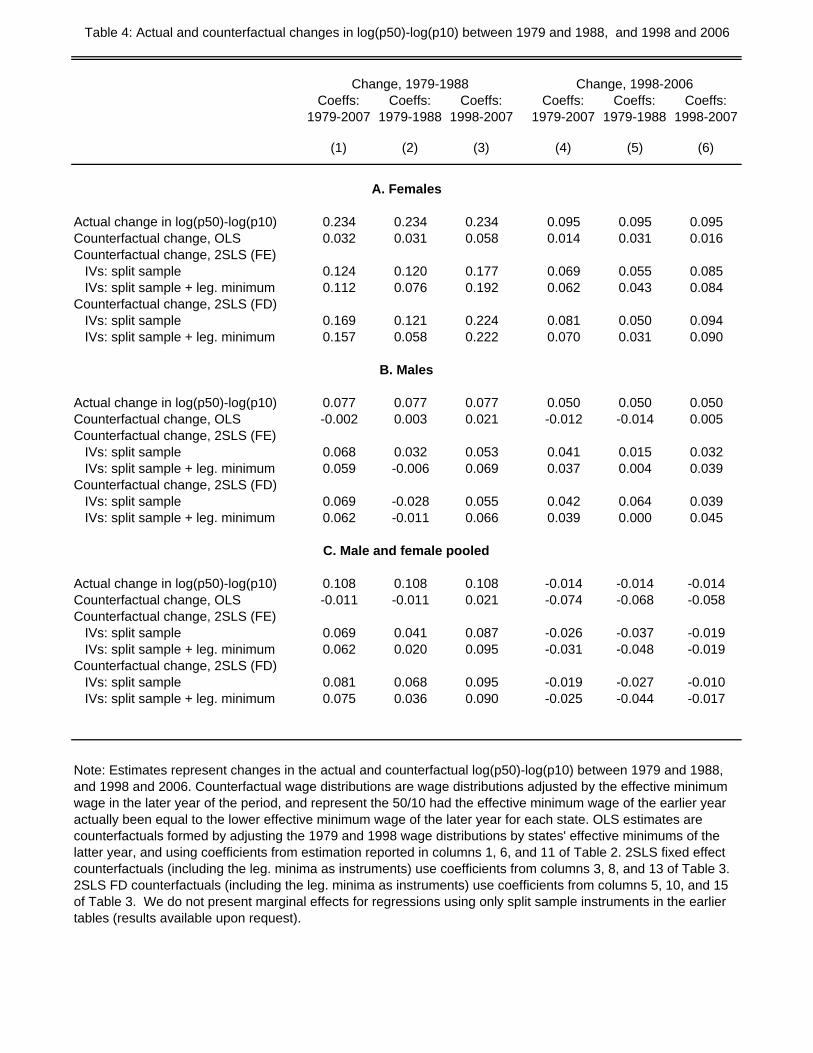
Coeffs: 1979-2007

Coeffs: 1979-1988

Coeffs: 1998-2007

Coeffs: 1979-2007

Coeffs: 1979-1988

Coeffs: 1998-2007

(1) (2) (3) (4) (5) (6)

Actual change in log(p50)-log(p10) 0.234 0.234 0.234 0.095 0.095 0.095Counterfactual change, OLS 0.032 0.031 0.058 0.014 0.031 0.016Counterfactual change, 2SLS (FE) IVs: split sample 0.124 0.120 0.177 0.069 0.055 0.085 IVs: split sample + leg. minimum 0.112 0.076 0.192 0.062 0.043 0.084Counterfactual change, 2SLS (FD) IVs: split sample 0.169 0.121 0.224 0.081 0.050 0.094 IVs: split sample + leg. minimum 0.157 0.058 0.222 0.070 0.031 0.090

Actual change in log(p50)-log(p10) 0.077 0.077 0.077 0.050 0.050 0.050Counterfactual change, OLS -0.002 0.003 0.021 -0.012 -0.014 0.005Counterfactual change, 2SLS (FE) IVs: split sample 0.068 0.032 0.053 0.041 0.015 0.032 IVs: split sample + leg. minimum 0.059 -0.006 0.069 0.037 0.004 0.039Counterfactual change, 2SLS (FD) IVs: split sample 0.069 -0.028 0.055 0.042 0.064 0.039 IVs: split sample + leg. minimum 0.062 -0.011 0.066 0.039 0.000 0.045

Actual change in log(p50)-log(p10) 0.108 0.108 0.108 -0.014 -0.014 -0.014Counterfactual change, OLS -0.011 -0.011 0.021 -0.074 -0.068 -0.058Counterfactual change, 2SLS (FE) IVs: split sample 0.069 0.041 0.087 -0.026 -0.037 -0.019 IVs: split sample + leg. minimum 0.062 0.020 0.095 -0.031 -0.048 -0.019Counterfactual change, 2SLS (FD) IVs: split sample 0.081 0.068 0.095 -0.019 -0.027 -0.010 IVs: split sample + leg. minimum 0.075 0.036 0.090 -0.025 -0.044 -0.017

Table 4: Actual and counterfactual changes in log(p50)-log(p10) between 1979 and 1988, and 1998 and 2006

A. Females

B. Males

C. Male and female pooled

Note: Estimates represent changes in the actual and counterfactual log(p50)-log(p10) between 1979 and 1988, and 1998 and 2006. Counterfactual wage distributions are wage distributions adjusted by the effective minimum wage in the later year of the period, and represent the 50/10 had the effective minimum wage of the earlier year actually been equal to the lower effective minimum wage of the later year for each state. OLS estimates are counterfactuals formed by adjusting the 1979 and 1998 wage distributions by states' effective minimums of the latter year, and using coefficients from estimation reported in columns 1, 6, and 11 of Table 2. 2SLS fixed effect counterfactuals (including the leg. minima as instruments) use coefficients from columns 3, 8, and 13 of Table 3. 2SLS FD counterfactuals (including the leg. minima as instruments) use coefficients from columns 5, 10, and 15 of Table 3. We do not present marginal effects for regressions using only split sample instruments in the earlier tables (results available upon request).

Change, 1979-1988 Change, 1998-2006

1979 1980 1981 1982 1983 1984 1985 1986 1987 1988 1989 1990 1991 1992 1993

Federal min. wage 2.90 3.10 3.35 3.35 3.35 3.35 3.35 3.35 3.35 3.35 3.35 3.80 4.25 4.25 4.25AlabamaAlaska 3.40 3.60 3.85 3.85 3.85 3.85 3.85 3.85 3.85 3.85 3.85 4.30 4.75 4.75 4.75ArizonaArkansasCalifornia 4.25 4.25 4.25ColoradoConnecticut 3.75 4.25 4.25 4.27 4.27 4.27DelawareFloridaGeorgiaHawaiiIdaho 3.85 3.85 3.85 4.75 5.25IllinoisIndianaIowaKansas 3.85 4.65 4.65KentuckyLouisianaMaineMaryland 3.45 3.55 3.65 3.65 3.75 3.85MassachusettsMichigan 3.65 3.65 3.75 3.75MinnesotaMississippi 3.55 3.85 3.95MissouriMontanaNebraskaNevadaNew HampshireNew Jersey 3.45 3.55 3.65New Mexico 5.05 5.05New YorkNorth CarolinaNorth DakotaOhioOklahomaOregonPennsylvania 4.25 4.75 4.75 4.75Rhode IslandSouth Carolina 3.55 3.65 4.00 4.25 4.25 4.45 4.45 4.45South DakotaTennesseeTexasUtahVermontVirginia 3.45 3.55 3.65 3.75 3.85WashingtonWest Virginia 3.85 3.85WisconsinWyoming 3.65

Appendix Table 1 - Variation in State Minimum Wages

Note: Table indicates years in which each state had a state minimum wage that exceeded the federal minimum wage for at least 6 months of the year.

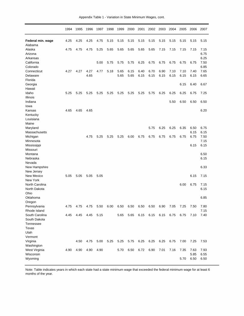
1994 1995 1996 1997 1998 1999 2000 2001 2002 2003 2004 2005 2006 2007

Federal min. wage 4.25 4.25 4.25 4.75 5.15 5.15 5.15 5.15 5.15 5.15 5.15 5.15 5.15 5.15AlabamaAlaska 4.75 4.75 4.75 5.25 5.65 5.65 5.65 5.65 5.65 7.15 7.15 7.15 7.15 7.15Arizona 6.75Arkansas 6.25California 5.00 5.75 5.75 5.75 6.25 6.75 6.75 6.75 6.75 6.75 7.50Colorado 6.85Connecticut 4.27 4.27 4.27 4.77 5.18 5.65 6.15 6.40 6.70 6.90 7.10 7.10 7.40 7.65Delaware 4.65 5.65 5.65 6.15 6.15 6.15 6.15 6.15 6.15 6.65FloridaGeorgia 6.15 6.40 6.67HawaiiIdaho 5.25 5.25 5.25 5.25 5.25 5.25 5.25 5.25 5.75 6.25 6.25 6.25 6.75 7.25IllinoisIndiana 5.50 6.50 6.50 6.50IowaKansas 4.65 4.65 4.65 6.20KentuckyLouisianaMaineMaryland 5.75 6.25 6.25 6.35 6.50 6.75Massachusetts 6.15 6.15Michigan 4.75 5.25 5.25 5.25 6.00 6.75 6.75 6.75 6.75 6.75 6.75 7.50Minnesota 7.15Mississippi 6.15 6.15MissouriMontana 6.50Nebraska 6.15NevadaNew Hampshire 6.33New JerseyNew Mexico 5.05 5.05 5.05 5.05 6.15 7.15New YorkNorth Carolina 6.00 6.75 7.15North Dakota 6.15OhioOklahoma 6.85OregonPennsylvania 4.75 4.75 4.75 5.50 6.00 6.50 6.50 6.50 6.50 6.90 7.05 7.25 7.50 7.80Rhode Island 7.15South Carolina 4.45 4.45 4.45 5.15 5.65 5.65 6.15 6.15 6.15 6.75 6.75 7.10 7.40South DakotaTennesseeTexasUtahVermontVirginia 4.50 4.75 5.00 5.25 5.25 5.75 6.25 6.25 6.25 6.75 7.00 7.25 7.53WashingtonWest Virginia 4.90 4.90 4.90 4.90 5.70 6.50 6.72 6.90 7.01 7.16 7.35 7.63 7.93Wisconsin 5.85 6.55Wyoming 5.70 6.50 6.50

Appendix Table 1 - Variation in State Minimum Wages, cont.

Note: Table indicates years in which each state had a state minimum wage that exceeded the federal minimum wage for at least 6 months of the year.

Figure 1A: Trends in state and federal minimum wages, and log(p10)-log(p50)

-.8-.7

-.6-.5

-.4-.3

-.2

Log(

p10)

-log(

p50)

1.6

1.7

1.8

1.9

22.

12.

2

Log

real

min

imum

wag

e, 2

007

dolla

rs

1974 1980 1985 1990 1995 2000 2005

Real value of average state/federal mins Real value of fed. min.

log(p10)-log(p50), female log(p10)-log(p50), male

Note: Annual data on state and federal minimum wages and log percentiles. Minimum wages are in 2007 dollars.

Figure 1B: Trends in state and federal minimum wages, and log(p90)-log(p50)

.5.6

.7.8

.91

1.1

Log(

p90)

-log(

p50)

1.6

1.7

1.8

1.9

22.

12.

2

Log

real

min

imum

wag

e, 2

007

dolla

rs

1974 1980 1985 1990 1995 2000 2005

Real value of average state/federal mins Real value of fed. min.

log(p90)-log(p50), female log(p90)-log(p50), male

Note: Annual data on state and federal minimum wages and log percentiles. Minimum wages are in 2007 dollars.

Figure 2: The theoretical relationship between deviations in the minimum and latent wage percentile, and differences between the minimum wage and latent percentile

Note: w(p)-w(p)* is the difference between the actual (observed) value of percentile p and the latent value of percentile p (i.e. its

w(p)-w(p)*

wm-w(p)*

Note: w(p) w(p) is the difference between the actual (observed) value of percentile p and the latent value of percentile p (i.e. its value in the absence of a minimum wage). wm-w(p)* is the difference between the minimum and the latent value of percentile p.

Figure 3: OLS and 2SLS estimates of the relationship between log(p)-log(p50) and log(min)-log(p50)Female wage distribution, 1979-2007

.5.6

.7

e)-lo

g(p5

0)A. OLS, levels (no state FE)

.5.6

.7

B. OLS, levels (state trends)

10

.1.2

.3.4

effe

ct o

f log

(min

. wag

10

.1.2

.3.4

-.3-.2

-.1

Mar

gina

l

0 5 10 15 20 25 30 35 40 45 50 55 60 65 70 75 80 85 90 95 100

-.3-.2

-.1

0 5 10 15 20 25 30 35 40 45 50 55 60 65 70 75 80 85 90 95 100

4.5

.6.7

age)

-log(

p50)

C. 2SLS, levels (state trends)

4.5

.6.7

D. 2SLS, first-differenced (state FE)

-.10

.1.2

.3.4

nal e

ffect

of l

og(m

in. w

a

-.10

.1.2

.3.4

-.3-.2

Mar

gin

0 5 10 15 20 25 30 35 40 45 50 55 60 65 70 75 80 85 90 95 100

Percentile

-.3-.2

0 5 10 15 20 25 30 35 40 45 50 55 60 65 70 75 80 85 90 95 100

Percentile

Note: Estimates are the marginal effects of log(min. wage)-log(p50), evaluated at the hours-weighted average of log(min. wage)-log(p50) across states and years. Observations are state-year observations. 95% confidence interval is represented by the dashed lines. Panel A corresponds with column 1 of Table 2. Panel B corresponds with column 3 of Table 2. Panel C corresponds with column 3 of Table 3. Panel D corresponds with column 5 of Table 3.

Figure 4: OLS and 2SLS estimates of the relationship between log(p)-log(p50) and log(min)-log(p50)Male wage distribution, 1979-2007

.5.6

.7

e)-lo

g(p5

0)A. OLS, levels (no state FE)

.5.6

.7

B. OLS, levels (state trends)

10

.1.2

.3.4

effe

ct o

f log

(min

. wag

e

10

.1.2

.3.4

-.3-.2

-.1

Mar

gina

l

0 5 10 15 20 25 30 35 40 45 50 55 60 65 70 75 80 85 90 95 100

-.3-.2

-.1

0 5 10 15 20 25 30 35 40 45 50 55 60 65 70 75 80 85 90 95 100

4.5

.6.7

age)

-log(

p50)

C. 2SLS, levels (state trends)

4.5

.6.7

D. 2SLS, first-differenced (state FE)

-.10

.1.2

.3.

nal e

ffect

of l

og(m

in. w

a

-.10

.1.2

.3.

-.3-.2

Mar

gin

0 5 10 15 20 25 30 35 40 45 50 55 60 65 70 75 80 85 90 95 100

Percentile

-.3-.2

0 5 10 15 20 25 30 35 40 45 50 55 60 65 70 75 80 85 90 95 100

Percentile

Note: Estimates are the marginal effects of log(min. wage)-log(p50), evaluated at the hours-weighted average of log(min. wage)-log(p50) across states and years. Observations are state-year observations. 95% confidence interval is represented by the dashed lines. Panel A corresponds with column 1 of Table 2. Panel B corresponds with column 3 of Table 2. Panel C corresponds with column 3 of Table 3. Panel D corresponds with column 5 of Table 3.

Figure 5: OLS and 2SLS estimates of the relationship between log(p)-log(p50) and log(min)-log(p50)Male and female wage distribution, 1979-2007

.5.6

.7

e)-lo

g(p5

0)A. OLS, levels (no state FE)

.5.6

.7

B. OLS, levels (state trends)0

.1.2

.3.4

effe

ct o

f log

(min

. wag

e

0.1

.2.3

.4

-.3-.2

-.1

Mar

gina

l e

0 5 10 15 20 25 30 35 40 45 50 55 60 65 70 75 80 85 90 95 100

-.3-.2

-.1

0 5 10 15 20 25 30 35 40 45 50 55 60 65 70 75 80 85 90 95 100

4.5

.6.7

ge)-l

og(p

50)

C. 2SLS, levels (state trends)

4.5

.6.7

D. 2SLS, first-differenced (state FE)

-.10

.1.2

.3.4

al e

ffect

of l

og(m

in. w

ag

-.10

.1.2

.3.4

-.3-.2

-

Mar

gina

0 5 10 15 20 25 30 35 40 45 50 55 60 65 70 75 80 85 90 95 100

Percentile

-.3-.2

-

0 5 10 15 20 25 30 35 40 45 50 55 60 65 70 75 80 85 90 95 100

Percentile

Note: Estimates are the marginal effects of log(min. wage)-log(p50), evaluated at the hours-weighted average of log(min. wage)-log(p50) across states and years. Observations are state-year observations. 95% confidence interval is represented by the dashed lines. Panel A corresponds with column 1 of Table 2. Panel B corresponds with column 3 of Table 2. Panel C corresponds with column 3 of Table 3. Panel D corresponds with column 5 of Table 3.

Figure 6: Actual and counterfactual change in log(p)-log(p50)Female wage distribution, 1979 to 1988

-.3-.2

-.10

.1C

hang

e in

log(

p)-lo

g(p5

0), 1

979-

1988

0 5 10 15 20 25 30 35 40 45 50 55 60 65 70 75 80 85 90 95 100Percentile

Actual change Cntfct. change, OLS

Cntfct. change, 2SLS (FE) Cntfct. change, 2SLS (FD)

Note: Plots represent the actual and counterfactual changes in the 5th through 95th percentiles of the female wage distribution. Counterfactual changes are calculated by adjusting the 1979 wage distributions by the value of states' effective minima in 1988 and coefficients from OLS regressions (column 1 of Table 2) and 2SLS first-differenced regressions (column 5 of Table 3).

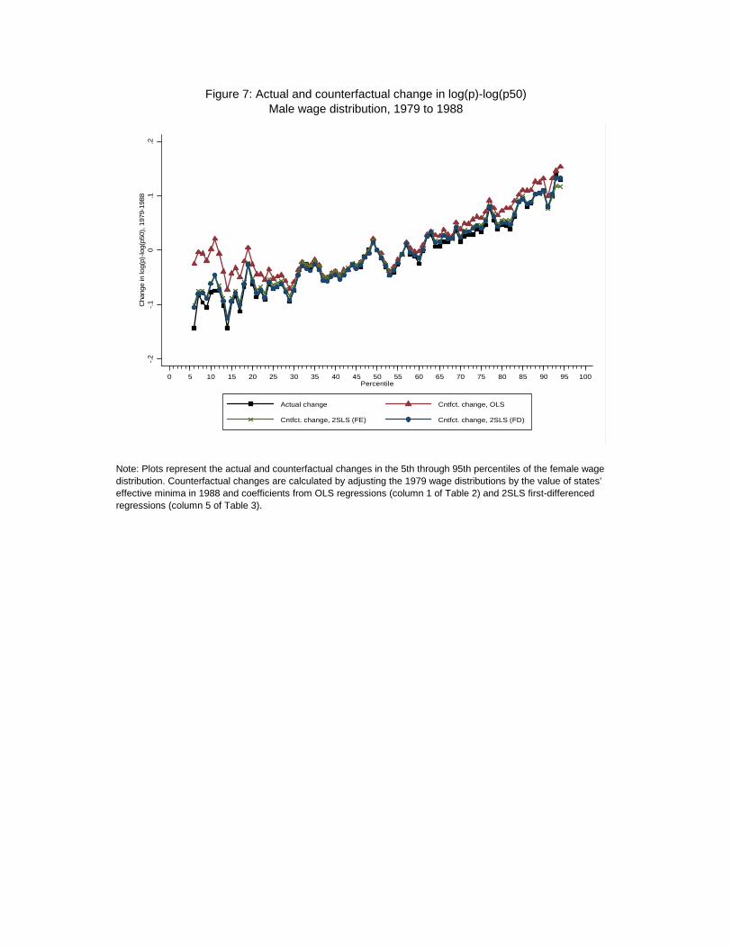
Figure 7: Actual and counterfactual change in log(p)-log(p50)Male wage distribution, 1979 to 1988

-.2-.1

0.1

.2C

hang

e in

log(

p)-lo

g(p5

0), 1

979-

1988

0 5 10 15 20 25 30 35 40 45 50 55 60 65 70 75 80 85 90 95 100Percentile

Actual change Cntfct. change, OLS

Cntfct. change, 2SLS (FE) Cntfct. change, 2SLS (FD)

Note: Plots represent the actual and counterfactual changes in the 5th through 95th percentiles of the female wage distribution. Counterfactual changes are calculated by adjusting the 1979 wage distributions by the value of states' effective minima in 1988 and coefficients from OLS regressions (column 1 of Table 2) and 2SLS first-differenced regressions (column 5 of Table 3).

Figure 8a: Actual and counterfactual change in log(p)-log(p50)Male and female pooled wage distribution, 1979 to 1988

.10

p)-lo

g(p5

0), 1

979-

1988

-.2-.1

Cha

nge

in lo

g(p

Figure 8b: Actual and counterfactual change in log(p)-log(p50)Male and female pooled wage distribution 1979 to 2007

0 5 10 15 20 25 30 35 40 45 50 55 60 65 70 75 80 85 90 95 100Percentile

Actual change Cntfct. change, OLS

Cntfct. change, 2SLS (FE) Cntfct. change, 2SLS (FD)

Male and female pooled wage distribution, 1979 to 2007

.1.1.2.2

979-

2007

979-

2007

-.1-.100

Cha

nge

in lo

g(p)

-log(

p50)

, 19

Cha

nge

in lo

g(p)

-log(

p50)

, 19

-.2-.2

00 55 1010 1515 2020 2525 3030 3535 4040 4545 5050 5555 6060 6565 7070 7575 8080 8585 9090 9595 100100PercentilePercentile

Actual changeActual change Cntfct. change, OLSCntfct. change, OLS

Cntfct. change, 2SLS (FE)Cntfct. change, 2SLS (FE) Cntfct. change, 2SLS (FD)Cntfct. change, 2SLS (FD)

Note: Plots represent the actual and counterfactual changes in the 5th through 95th percentiles of the female wage distribution. Counterfactual changes are calculated by adjusting the 1979 and 2007 wage distributions by the value of states' effective minima in 1988 and coefficients from OLS regressions (column 1 of Table 2), 2SLS levels regressions with state trends (column 3 of Table 3), and 2SLS first-differenced regressions (column 5 of Table 3).

Figure 9 - Average difference between actual and latent percentiles

.1.1

5.2

actu

al p

erce

ntile

- la

tent

per

cent

ile

0.0

5

Ave

rage

a

0 5 10 15 20 25 30 35 40 45 50 55 60 65 70 75Percentile

Female Male

Pooled

Note: Deviations are averaged across all states and years. See text for description of how devs. are computed.

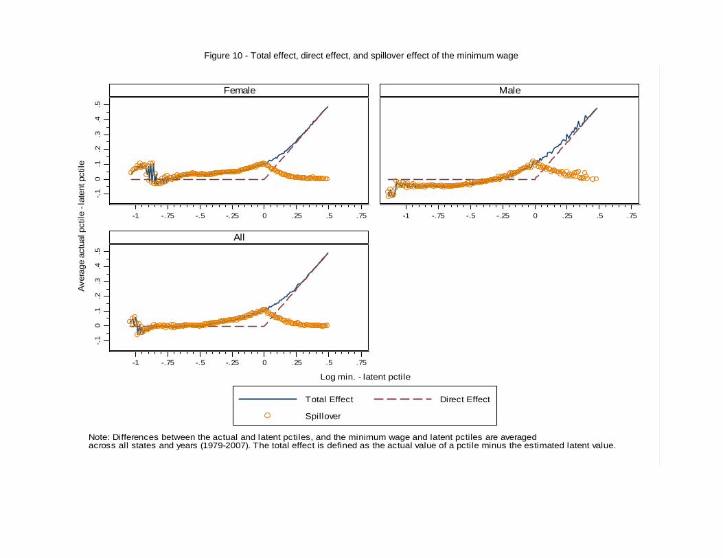
Figure 10 - Total effect, direct effect, and spillover effect of the minimum wage

-.1

0.1

.2.3

.4.5

.5

-1 -.75 -.5 -.25 0 .25 .5 .75 -1 -.75 -.5 -.25 0 .25 .5 .75

Female Male

All

e ac

tual

pct

ile -

late

nt p

ctile

-.1

0.1

.2.3

.4

-1 -.75 -.5 -.25 0 .25 .5 .75

Total Effect Direct Effect

Spillover

Ave

rage

Log min. - latent pctile

Note: Differences between the actual and latent pctiles, and the minimum wage and latent pctiles are averagedacross all states and years (1979-2007). The total effect is defined as the actual value of a pctile minus the estimated latent value.

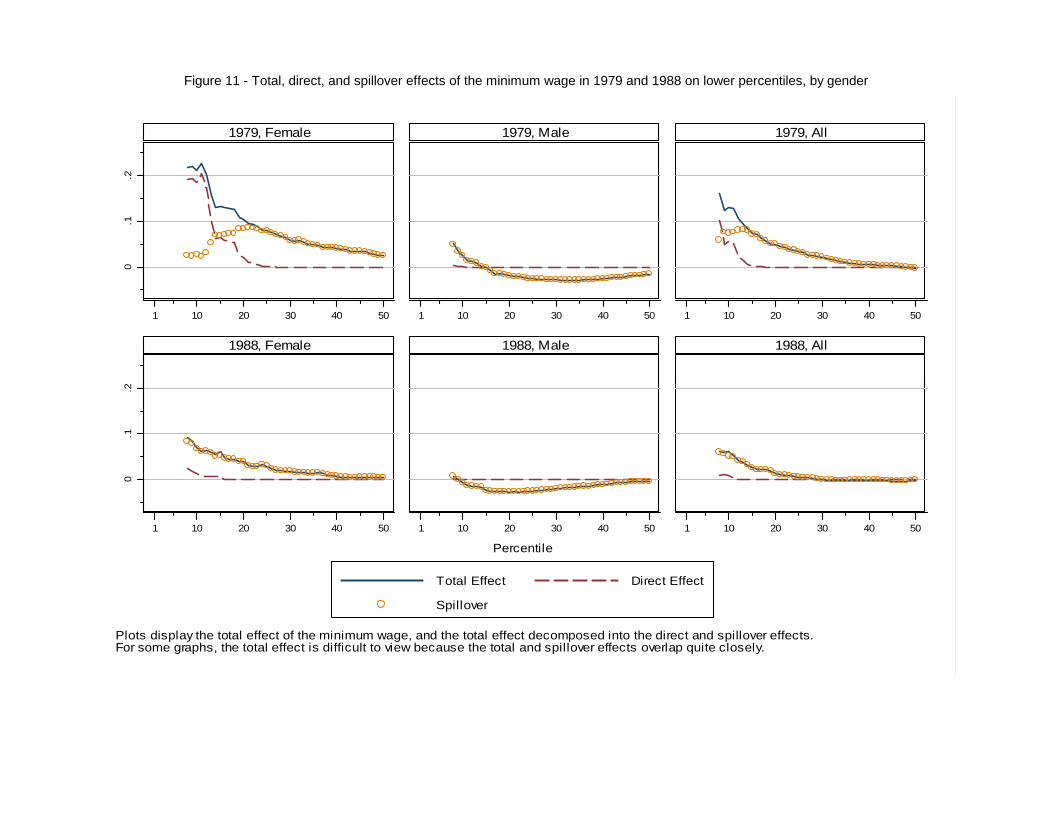
Figure 11 - Total, direct, and spillover effects of the minimum wage in 1979 and 1988 on lower percentiles, by gender

0.1

.2

1 10 20 30 40 50 1 10 20 30 40 50 1 10 20 30 40 50

1979, Female 1979, Male 1979, All

1988, Female 1988, Male 1988, All

0.1

.2

1 10 20 30 40 50 1 10 20 30 40 50 1 10 20 30 40 50

Total Effect Direct Effect

Spillover

Percentile

Plots display the total effect of the minimum wage, and the total effect decomposed into the direct and spillover effects.For some graphs, the total effect is difficult to view because the total and spillover effects overlap quite closely.

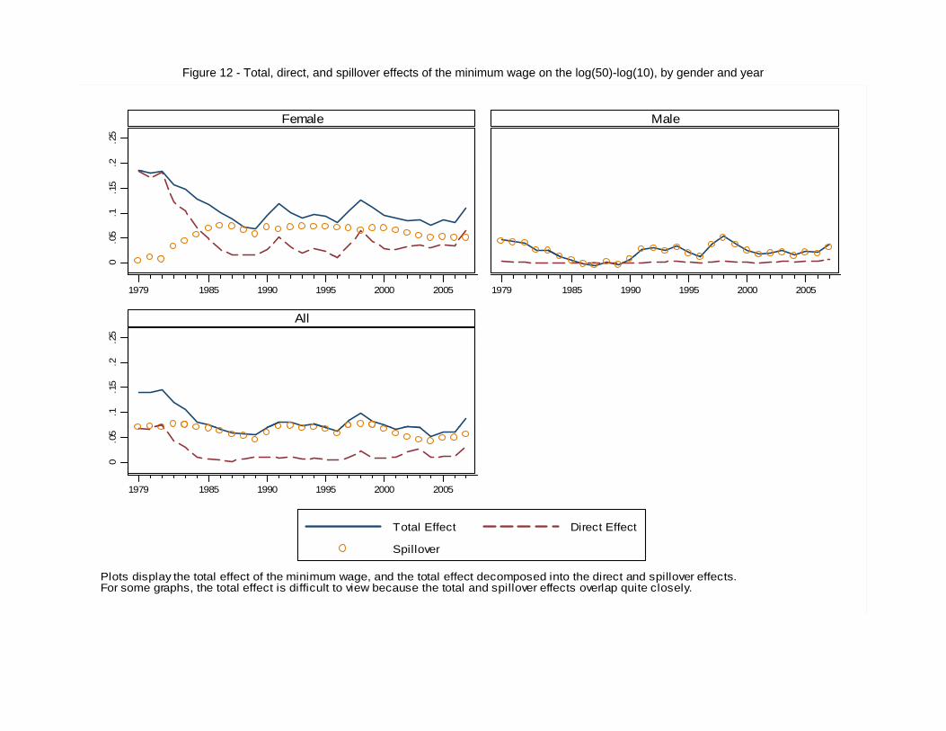
Figure 12 - Total, direct, and spillover effects of the minimum wage on the log(50)-log(10), by gender and year

.2.2

5Female Male

.05

.1.1

50

25

1979 1985 1990 1995 2000 2005 1979 1985 1990 1995 2000 2005

All

.1.1

5.2

.0

.05

1979 1985 1990 1995 2000 2005

Total Effect Direct Effect

Spillover

Plots display the total effect of the minimum wage, and the total effect decomposed into the direct and spillover effects.For some graphs, the total effect is difficult to view because the total and spillover effects overlap quite closely.

Figure 13 - Estimates of the probability of correctly reporting the wage, by gender and year

Note: p1 indicates probability for women, p2 is the probability for males, and p3 is the probability for the pooled sample.

Figure 14 - Estimates of the effect of the min. on the mean, and bounds for the size of the spike at the min. wage in the absence of spillovers

.15

Female Male0

.05

.1

mea

n

05

1979 1985 1990 1995 2000 2005 1979 1985 1990 1995 2000 2005

Pooled

min

imum

wag

e on

m

05.1

.15

Effe

ct o

f m

0.0

1979 1985 1990 1995 2000 2005

Bounds on size of true spike, assuming no spillovers Estimated effect of min on mean

Plots display the estimated average marginal effects of the minimum wage on the mean, and the upper and lower bounds for the size of thetrue spike assuming no spillovers.