the role of black holes in the ads/cft correspondence · theory. the ads/cft correspondence is...
TRANSCRIPT
THE ROLE OF BLACK HOLES IN THE ADS/CFT
CORRESPONDENCE
Jakob Gath
Submitted in partial fulfilment of the requirements for the degree of
Master of Science of the Imperial College London
Imperial College London
MSc Dissertation
25th of September 2009
Abstract
The two descriptions of low energy dynamics of coincident branes are
considered. One description is the supergravity approximation of the su-
perstring theory where the extremal black p-brane solution emerges. The
other description consist of a gauge theory which describes the dynamics
of the world volume of the N coincident branes. The AdS/CFT conjecture
is introduced and the important equivalence of the two theories’ partition
functions. By the identification that the UV limit of the field theory corre-
sponds to the boundary of five dimensional anti-de Sitter space, the principle
of holography is introduced. To evaluate the partition function the saddle-
point approximation is used. However, since the action is divergent due to
the infinite volume of asymptotically anti-de Sitter spacetimes, a renormali-
sation scheme is needed. This is carried out by two different methods. First,
the method of holographic renormalisation is used to define a renormalised
action and to extract the stress-energy tensor of the field theory on the
boundary of the asymptotically anti-de Sitter spacetimes. Secondly, a finite
action is obtained by performing a background subtraction. In the latter
method, a detailed analysis is performed in order to determine the thermo-
dynamical favourable spacetime configuration as a function of temperature.
It is found that a phase transition occurs from thermal anti-de Sitter space
to a configuration with a black hole. For the strongly coupled dual field
theory in the large N limit, this is interpreted as a phase transition from a
confined phase to a deconfined phase.

Contents
1 Introduction 1
2 Supergravity and Gauge Theory 5
2.1 Extremal Black p-Branes . . . . . . . . . . . . . . . . . . . . . 6
2.2 Non-Abelian Gauge Theory on D-branes . . . . . . . . . . . . 12
2.3 D3-branes; Conformal N = 4 Super Yang-Mills . . . . . . . . 13
3 Anti-de Sitter / Conformal Field Theory 16
3.1 Decoupling in the gsN 1 Limit . . . . . . . . . . . . . . . . 16
3.2 Decoupling in the gsN 1 Limit . . . . . . . . . . . . . . . . 17
3.3 Conjecture . . . . . . . . . . . . . . . . . . . . . . . . . . . . . 19
3.4 Holographic Duality . . . . . . . . . . . . . . . . . . . . . . . 21
4 Finite Temperature 24
4.1 The Saddle-Point Approximation . . . . . . . . . . . . . . . . 25
4.2 Near-extremal D3-brane . . . . . . . . . . . . . . . . . . . . . 26
4.3 Global Coordinates . . . . . . . . . . . . . . . . . . . . . . . . 28
4.4 The Conformal Boundary . . . . . . . . . . . . . . . . . . . . 29
4.5 Holographic Renormalisation . . . . . . . . . . . . . . . . . . 31
5 Thermal Phase Transition in Anti-de Sitter Space 38
5.1 Criterion for Confinement/Deconfinement . . . . . . . . . . . 39
5.2 Schwarzschild Black Hole in Anti-de Sitter Space . . . . . . . 39
5.3 The Periodicity of Imaginary Time . . . . . . . . . . . . . . . 42
5.4 Two Black Hole Sizes . . . . . . . . . . . . . . . . . . . . . . 44
5.5 Actions and Partition Functions . . . . . . . . . . . . . . . . 45
5.6 Energy, Specific Heat Capacity . . . . . . . . . . . . . . . . . 48
5.7 Phase Transition . . . . . . . . . . . . . . . . . . . . . . . . . 51
5.8 Entropy and Field Theory . . . . . . . . . . . . . . . . . . . . 53
i
6 Conclusion 56
Appendices 60
A Maximally Symmetric Spacetimes 60
A.1 The Cosmological Constant . . . . . . . . . . . . . . . . . . . 61
A.2 Anti-de Sitter Spacetime . . . . . . . . . . . . . . . . . . . . . 62
A.3 Global Coordinates . . . . . . . . . . . . . . . . . . . . . . . . 64
A.4 Poincare Coordinates . . . . . . . . . . . . . . . . . . . . . . . 66
A.5 Additional Mapping . . . . . . . . . . . . . . . . . . . . . . . 67
A.6 The Causal Structure . . . . . . . . . . . . . . . . . . . . . . 68
A.7 Geodesics in Global Coordinates . . . . . . . . . . . . . . . . 69
A.8 Physics and Initial Configurations . . . . . . . . . . . . . . . 71
B String Theory 72
B.1 The Massless Content . . . . . . . . . . . . . . . . . . . . . . 74
B.2 Double Expansion . . . . . . . . . . . . . . . . . . . . . . . . 76
B.3 Supergravity Actions . . . . . . . . . . . . . . . . . . . . . . . 77
B.4 The Brane Spectrum . . . . . . . . . . . . . . . . . . . . . . . 79
B.5 S-duality . . . . . . . . . . . . . . . . . . . . . . . . . . . . . . 81
C Statistical Mechanics 83
C.1 The Path Integral . . . . . . . . . . . . . . . . . . . . . . . . 84
D The Theory of Black Holes 88
D.1 Uniqueness Theorems . . . . . . . . . . . . . . . . . . . . . . 88
D.2 Classical Black Hole Solutions . . . . . . . . . . . . . . . . . . 89
D.3 Black Hole Properties . . . . . . . . . . . . . . . . . . . . . . 90
D.4 Black Hole Thermodynamics . . . . . . . . . . . . . . . . . . 91
D.5 The Chain of Assumptions . . . . . . . . . . . . . . . . . . . . 99
D.6 Notion of Symmetry in General Relativity . . . . . . . . . . . 100
ii

1 Introduction
String theory is one of the most promising candidates that theoretical physi-
cists have for a consistent unifying theory of the forces of nature. Surpris-
ingly, it was found that string theory is not only a theory of strings, but,
in fact, also of spatially extended objects called branes. There are two low
energy descriptions of branes. The supergravity approximation that yields
an effective action for which the geometry of branes can be solved for, and a
U(N) gauge theory that describes the dynamics of the world volume of the
branes. It is from these two descriptions that the gauge/gravity dualities
arise. A duality relates a strongly coupled theory to a dual weakly coupled
theory.
A particularly interesting gauge theory is QCD, which is based on the
gauge group SU(3). QCD is a quantum field theory where the basic con-
stituents of hadrons are quarks and gluons. It is the theory used to describe
the strong forces and is an asymptotically free theory which means that
the cutoff ΛQCD decreases as the energy increases. At low energy it is thus
strongly coupled. With a gauge/gravity duality, it becomes possible to ap-
proach the intractable strongly coupled regime of the theory by performing
perturbation theory at weak coupling in the dual gravity theory. Although
the dual string theory for QCD is not yet known, it is believed to exist. Cur-
rently, dualities that relate their conformal invariant cousins with a SU(N)
gauge group to string theory are considered. These gauge theories are often
supersymmetric with a large number of degrees of freedom, that is, large N .
Nonetheless, qualitative predictions for more realistic theories, like QCD,
can still be made.
In this text, a duality known as a AdS/CFT correspondence is ap-
proached in the form where the type IIB superstring theory on the max-
imally symmetric AdS5 × S5 background is related to the four dimensional
supersymmetric N = 4 Yang-Mills gauge theory with gauge group SU(N).
1
Anti-de Sitter space is the maximally symmetric solution of Einstein’s equa-
tions with a negative cosmological constant, and the four dimensional gauge
theory is a conformal invariant theory; that is, it has a vanishing beta func-
tion. Since string theory, and in particular the type IIB theory, plays such a
dominant role, appendix B provides a general introduction and gives, among
other things, the massless spectrum and the brane spectrum of the type IIB
theory. The AdS/CFT correspondence is quite remarkable, as already men-
tioned, since it relates a theory of gravity, which string theory is, to a theory
with no gravity at all. It should, however, be kept in mind at this point that
it is only conjectured, not proven.
When matching spacetime coordinates of the two theories, it emerges
that the UV limit of the gauge theory corresponds to the conformal bound-
ary structure of anti-de Sitter space. This is the limit where field theories
are usually discussed, which is why the field theory is said to live on the
boundary of anti-de Sitter space. This picture is called a holographic dual-
ity because the higher dimensional physics in anti-de Sitter space is encoded
in the lower dimensional field theory. It turns out, however, that the choice
of coordinates introduces an ambiguity because it leads to different confor-
mal structures of the boundary. However, this choice is simply a choice of
regulator at a given energy scale when renormalising the divergent action of
anti-de Sitter space. The negative curved anti-de Sitter space has a number
of natural choices of coordinates, for which appendix A is provided.
The correspondence can be generalised to a duality between type IIB
on asymptotic anti-de Sitter backgrounds and a dual gauge theory based
on considerations of near-extremal solutions of supergravity. The interior of
such backgrounds can, among other things, contain black holes. Black holes
have a vast history of thermodynamical analogy for which a detailed review
is given in appendix D. The analogy means that it is possible to introduce
a temperature in the correspondence. This opens for an approach to make
2
predictions in the strongly coupled field theory at finite temperatures. A
finite temperature has the implication of introducing an energy scale in the
field theory, which breaks its conformal invariance.
Along with the correspondence, the equivalence of the two theories’ par-
tition functions are likewise conjectured [29]. From the Euclidean path in-
tegral approach towards quantum gravity, which provides a semi-classical
prescription for evaluating the thermodynamical partition function of the
gravity theory, the stable and favourable spacetime configurations as a func-
tion of temperature can be determined. In doing so, one considers the
positive-definite sections of the contributing metrics, which are obtained by
performing a Wick rotation. In contrast to the anti-de Sitter metric, the
black hole metric admits a unique spin structure corresponding to a ther-
mal (anti-periodic) boundary condition, which is supersymmetry-breaking.
The relation between the Euclidean path integral and the partition func-
tion of the canonical ensemble is reviewed in appendix C. Having the most
favourable spacetime configuration as a function of temperature, possible
phase transitions are directly predictable and can be mapped to the strongly
coupled dual gauge theory at large N . In fact, one finds that the gauge the-
ory in question undergoes a transition from a confined phase consisting of
singlet hadrons to a deconfined phase of quark-gluon plasma. Interestingly,
this plasma, in the case of QCD, has been observed briefly at the experi-
ments at the Relativistic Heavy Ion Collider (RHIC) [32], [4].
The two low energy descriptions of N coincident branes are introduced in
section 2. In particular, the extremal black 3-brane solution of supergravity,
which turns out to have the special near-horizon geometry of AdS5×S5, and
the four dimensional gauge theory living on the the D3-branes, which turns
out to have the special property of conformal invariance. Looking at the
descriptions in their respective limits of validity at low energies in section 3,
3

the AdS/CFT correspondence considered here is introduced. A discussion
of the holographic nature of the duality will also be given. In section 4 it
is shown how a finite temperature in the correspondence arises from the
black hole geometry of the near-extremal black 3-brane. Furthermore, the
divergent action due to the infinite volume of anti-de Sitter spacetime and
the need for a renormalisation are discussed. The method of holographic
renormalisation is used in section 4.5 to extract the boundary stress-energy
tensor of the anti-de Sitter and Schwarzschild-AdS spacetimes. This also
spawns an elaborate discussion of the impact the choice of coordinates has
on the theory. Hereafter, the N = 4 gauge theory on the spatial manifold
S3 shall be considered at finite temperature. To study this theory at finite
temperatures, the thermodynamical partition function is determined on S1×
S3 by Euclideanising the spacetime metrics and evaluating the saddle-point
approximation of the Euclidean path integral. Having the partition function
makes it possible to compute the thermodynamical properties of the black
hole in anti-de Sitter space and compare it to the empty anti-de Sitter space.
Finally, the results are compared to the expected behaviour of the dual field
theory.
The units are chosen such that c = ~ = k = 1 while Newton’s constant
GN is kept.
4

2 Supergravity and Gauge Theory
As hinted in appendix B, there exist two descriptions of the low energy
dynamics of branes. One description treats the brane as a source for the
closed string fields in superstring theory and is a solution to the low energy
field equations derived from supergravity. The other description uses the
dynamics of the world volume field theory of N coincident Dp-branes. In
both cases, it is important to identify valid regimes. First, recall that there
exists a whole tower of stringy dynamics on top of the low energy physics,
whose influence is made insignificant when α′ → 0. In addition, working
with small gs ensures that one remains in the classical supergravity regime,
that is at the string tree level. Also, in the weak-coupling regime it is evident
from the tension of the D-brane that one can treat them as rigid objects and
therefore the truncation of the world volume effective actions can be trusted.
The two descriptions are essential for the understanding of the conjecture
of the duality between gauge theory and gravity.
In the following section, the extremal black p-brane solutions of the type
II supergravity actions shall be considered. The case of p = 3 turns out to
be particular interesting in that it, among other things, has a finite horizon
area. The solution arises from the self-dual four-form gauge potential in
the type IIB R-R sector and its near-horizon geometry turns out to be
AdS5×S5. Later, when more is understood, the non-extremal black 3-brane
solution will be considered. It will turn out to have a Schwarzschild-anti-
de Sitter black hole times a five-sphere geometry. In section 2.2 and 2.3,
the open string sectors and coincident D-branes shall be considered. This
gives a U(N) gauge theory, and of particular interest is the world volume
field theory of N coincident D3-branes which is the four dimensional N = 4
supersymmetric Yang-Mills theory with SU(N) gauge group.
5
2.1 Extremal Black p-Branes
This section will show how the anti-de Sitter space emerges in the AdS/CFT
correspondence. Considering the type II supergravity approximation, solu-
tions are obtained for the weak-coupling gs 1 regime where strings are
propagating in a fixed background. The solutions will turn out to be similar
to the charged Reissner-Nordstrom solutions known from general relativity
(see section D.2). They are, however, extended in p spatial directions and
because they have an event horizon they are called black p-branes. In par-
ticular, the focus here will be on the case of imposing the extremal condition
on the general p-brane solution. Recall that extremal objects in general rel-
ativity are defined by M = Q and as a consequence have zero temperature1.
This is similar for the higher dimensional p-brane generalisations. The ex-
plicit form of a general p-brane solution is not relevant for the discussion,
but can be found in various references (see e.g. [17], [1]). Finally, it should
be mentioned that although the supergravity solution is the description used
to describe low energy string theory, it is believed that the solution may be
extended to the full type II string theory. Although, it will of course have
α′ corrections of the metric and other fields.
As for the black hole solutions in four dimensions, which are solutions
to the equations of motion of the Einstein-Hilbert action, one is similarly
considering the solutions to the equations of motion derived from the Type
II supergravity action. To construct an extremal black p-brane it is only
necessary to include one field from the R-R sector in the action, say Cp+1
(see section B.1). One finds a family of ten dimensional solutions which
sources gravity, the dilaton, and the R-R gauge potential. The two-form
term from the NS-NS sector vanishes. Let the field strength of the R-R
sector field be Fp+2 = dCp+1 and Φ be the dilaton then the string-frame
1The extremal condition is given from the definition of the action given by equation
(1) and does therefore not include a factor of√
GN.
6
action takes the form [4]
S(p) =1
2κ20
∫d10x√−g[e−2Φ(R+ 4(∂Φ)2)− 1
2|Fp+2|2
], (1)
where κ0 is given by equation (74). The case of p = 3 is special because the
field strength arising from the R-R four-form of Type IIB is self-dual. To
ensure this is satisfied, it is necessary to impose the additional constraint
F5 = ?F5 ,
and introduce an additional factor of 1/2 in front of the |F5|2 term. The
solution for the extremal black p-brane metric is
ds2 = H− 1
2p (ηµνdxµdxν) +H
12p
(dr2 + r2dΩ2
8−p)
. (2)
The part in the first parenthesis is the flat Lorentzian metric in p + 1 di-
mensions while the part in the second parenthesis is an Euclidean metric in
9− p dimensions. This is consistent with the fact that placing an extremal
p-brane in spacetime breaks Lorentz symmetry,
SO(9, 1)→ SO(p, 1)× SO(9− p) , (3)
where the first factor is the Lorentz symmetry along the brane while the
second factor is the rotation symmetry for the perpendicular directions.
Since there is rotational symmetry in the 9 − p transverse directions, it is
possible to use spherical coordinates with a radial coordinate r and angular
coordinates on a (8− p)-sphere.
The function Hp present in the metric is the harmonic function that
solves the (9 − p)-dimensional Laplace equation. Extremal black p-branes
are defined by these harmonic functions which are functions of the radial
coordinate r,
Hp(r) = 1 +(rpr
)7−p. (4)
The solution is thus parametrized by the positive parameter rp to be deter-
mined later. From the dilaton’s equation of motion one finds the solution
eΦ = gsH3−p4
p ,
7

from which it is seen that the dilaton field is spatially varying for all values
of p except p = 3. From the behaviour Hp → 1 as r → ∞ of the harmonic
function gs defines the string coupling at infinity. This behaviour also shows
that the metric is asymptotically flat. For p < 3, it is evident that the system
goes into the nonperturbative regime for r → 0. This means eΦ becomes
large for which the classical supergravity solution is unreliable. Interestingly,
for the special case of p = 3 the dilaton is seen to be constant and thus the
string coupling is given by gs for all r.
One can generalise to a multicentre solution by writing the harmonic
function as
Hp(r) = 1 +k∑i=1
(rp
|~r − ~ri|
)7−p, (5)
which represents k parallel extremal p-branes located at arbitrary positions
given by ~ri. For this particular form, each brane carries Ni unit of R-R
charge and the total charge is the integer N . In the following, a single brane
with N R-R charges is considered. From the equation of motion of the R-R
field one finds
Cp+1 = (H−1p − 1)dx0 ∧ ... ∧ dxp
Fp+2 = dH−1p ∧ dx0 ∧ ... ∧ dxp .
Since the brane will generate a flux of the corresponding p+2 field strength,
one must be able to express the above equation for the field strength by the
following
Fp+2 =
Q(ω5 + ?ω5) for p = 3
Q ? ω8−p otherwise,
where Q is the D-brane charge per unit volume and ωn is the volume form
of a n-sphere. Note that the special case of p = 3 is due to the self-dual field
strength. This particular form ensures that the integration over the dual
field strength ?F yields the charge [1]∫S8−p
?Fp+2 = QΩ8−p = N , (6)
8
where N is the R-R charge of the brane. The volume of a n-sphere is
Ωn = Vol(Sn) =2π
n+12
Γ(n+1
2
) . (7)
One can express the parameter rp in terms of gs and N from equation (6).
Alternatively, it can be done by matching the metric (2) with the form of a
Schwarzschild black hole with mass M in ten dimensions. In the Einstein-
frame, the time-time component h reads [4]
h = 1− r20
rd−3, r2
0 =16πG(d)
N M
(d− 2)Ωd−2. (8)
However, in order to match this result with the corresponding term in the
string-frame metric, an appropriate transformation of metric and dilaton
must be performed (see e.g. [17]). This reveals that if the Hp is given by
equation (4) with d = 10− p, then [23]
rd−3p =
16πG(d)N M
(d− 3)Ωd−2. (9)
The mass of the extremal p-brane wrapped around a p-dimensional compact
space of volume Vp can be expressed in terms of the tension and charge of a
Dp-brane as
M = NTDpVp, TDp =1
(2π)pgs`p+1s
.
At infinity in the reduced (d− p)-dimensional spacetime the brane appears
as a point source of mass M . Newton’s constant in ten dimensions is related
to the (d− p)-dimensional one by
G(d−p)N =
G(d)N
Vp, G
(10)N = 8π6g2
s`8s . (10)
From the two last relations, one has
G(d−p)N M = G
(d)N NTDp ,
which, when substituted into equation (9) with d = 10− p, yields a relation
between the parameter rp in units of string length and gsN(rp`s
)7−p= (2√π)5−pΓ
(7− p
2
)gsN . (11)
9

For a general p the squared curvature invariant is proportional to either
side of this equation. For rp much larger than the string length `s, that is
gsN 1, the supergravity description can therefore be trusted. Further
discussion of this equation in the case of p = 3 is addressed later. For all p
except for p = 3, the horizon at r = 0 is a singular place of zero area, since
the radius of S8−p vanishes there. The metric therefore only describes the
spacetime outside the horizon. The 3-brane is of interest for various reasons;
its world volume has four dimensional Poincare invariance, it is self-dual, and
the horizon has finite area. In addition, the dilaton is constant throughout
spacetime, which simplifies the above relation, setting r3 = b and the string
length `s =√α′ (see section B.2), one has
b4 = 4πgsNα′2 . (12)
The near-horizon of the 3-brane is also particularly interesting because it
describes the low energy physics as shown in section 3.2. In the near-horizon
region r b, the harmonic function can be approximated by
H3(r) ≈(b
r
)4
, (13)
and thus the geometry of the near-horizon can is found
ds2 ≈(rb
)2(ηµνdxµdxν) +
(b
r
)2 (dr2 + dΩ2
5
). (14)
Making a variable substitution z = b2/r reveals the familiar form of anti-de
Sitter spacetime in local coordinates (see equation (68))
ds2 ≈ b2
z2
[ηµνdx
µdxν + dz2]
+ b2dΩ25 . (15)
More precisely this is five dimensional anti-de Sitter space times a five-sphere
AdS5 × S5 where the parameter b is identified as the radius of both. The
anti-de Sitter part is the primary focus and is reviewed in some details in
appendix A. The constant Ricci curvature of AdS is given by the radius of
curvature in equation (60)
R ∝ − 1b2
. (16)
10

With this equation and constant string coupling gs it is now possible to
compare scales with the coupling constant gsN . Above, the black p-brane
solutions have only been treated using classical supergravity. This requires
that the curvature is small compared to the string length. By equation (12)
and thus equation (16) this implies that b is much larger than the string
length. To suppress string loops one also needs to be in the weak-coupling
regime gs 1, that is the regime of string perturbation theory. This is
possible provided that N is sufficiently large. However, if the string coupling
is large, one could also use S-duality gs → 1/gs (see section B.5). In the
p = 3 case where the horizon is not singular, the solution can, in fact, be
analytically extended beyond r = 0. The maximally extended metric does
not have a singularity and is geodesically complete [1]. The supergravity
approximation in the case of p = 3 is thus reliable when
N > gsN 1 .
Stringy corrections are thus suppressed for gsN 1 and quantum correc-
tions are small when N 1 provided gsN is fixed. The ten dimensional
Planck length is related to the string length by `4p = gs`4s, thus equation (12)
can be expressed as (b
`p
)4
= 4πN .
This means that b must be much larger than the Planck length `p.
Besides the low energy limit of supergravity α′ → 0, the other expan-
sion regime of string theory is that of weak coupling gs → 0. In this case,
equation (5) shows via equation (11) for gsN 1 that the metric for co-
incident branes essentially becomes flat everywhere except on the (p + 1)-
dimensional hypersurface given by ~r = 0, where the metric appears to be
singular. Strings propagating on this background are thus moving in flat
spacetime, except when the string reaches the brane.
11

2.2 Non-Abelian Gauge Theory on D-branes
A Dp-brane is a (p + 1)-dimensional hypersurface in spacetime. They are
charged under a p+ 1 gauge field, which is part of the massless closed string
modes present in the supergravity multiplet derived for type IIB in section
B.1. Note that this spectrum was derived in flat space before any D-branes
were present. The branes are therefore sources of closed strings and can have
open strings ending on them. The brane spectrum for type IIB is discussed
in section B.4. A description of weak-coupling exists and is addressed now.
In the weak-coupling regime where the string coupling gs is taken to
be small, string perturbation theory becomes possible (see section B.2). In
this case, a D-brane becomes much heavier than the fundamental string (see
section B.4) and is taken to be rigid surfaces where open strings can end,
inducing a U(1) gauge theory on the world volume. Branes are thus viewed
as point-like in their transverse directions in otherwise flat space. Multiple
coincident D-branes allow open strings to start on one brane and end on
another by placing Chan-Paton matrices λaij on the ends [4]. For N branes
N2 − N string configurations are possible. In this case, the effective loop
expansion parameter for the open strings is gsN rather than gs. The D-
brane description is therefore valid for gsN 1. If the ends of the open
string are labelled i and j, the massless open string state can be shown to
be a vector
|µ〉 ⊗ |i〉 ⊗ |j〉 ,
which is a gauge field Aaµ of the U(N) gauge group. The λaij are genera-
tors of the adjoint representation. In the coincident case, the U(1)N is thus
enhanced to U(N). In the limit α′ → 0, only the massless states of the
open strings remain and they describe oscillations and the gauge field on
the branes. In this limit, the gauge theory is free. When only the dynamics
on the branes are of interest, the overall factor U(1) = U(N)/SU(N), which
determines the position of the branes, can be ignored. This leaves a SU(N)
12
gauge symmetry. Superstring theory has 32 supercharges, which form eight
four-dimensional spinors; that is, N = 8 in four dimensions. Placing co-
incident D-branes in spacetime breaks translation invariance and therefore
breaks half of the supersymmetry. The fields on the world volume of the
coincident D-branes are those of a maximally symmetric vector multiplet for
spins less or equal to one: gauge fields, scalars, and spinors, all in the adjoint
representation of SU(N). The non-trivial terms in a weak-field expansion
are thus exactly N = 4 super Yang-Mills.
2.3 D3-branes; Conformal N = 4 Super Yang-Mills
In this section some essential properties of the SU(N) gauge theory living on
the four dimensional world volume of N coincident D3-branes are discussed.
For more extensive reviews see [1], [19], or [7].
From the previous section, it is evident that the four dimensional gauge
theory living on the coincident D3-branes is the supersymmetric Yang-Mills
theory with N = 4 supercharges and gauge group SU(N). In general, it
is difficult to find quantum field theories which are conformally invariant.
However, this is exactly the case for this particular theory. This comes from
the fact that its beta function vanishes everywhere, which implies that there
is a cancellation of UV divergences to all orders in perturbation theory.
The need for introducing a renormalisation scale is therefore not necessary.
One is, however, free to define the theory at a particular energy scale E
by integrating out all degrees of freedom above that scale. For the case of
super Yang Mills theory in p + 1 dimensions the effective coupling can be
determined by dimensional analysis
g2eff(E) ∼ g2
YMNEp−3 .
For p = 3, the coupling is seen to be independent of the energy scale and is
known as the ’t Hooft coupling λ = g2YMN . It should be mentioned that the
13

open string coupling constant coincides with gYM. In the case of p = 3, the
N = 4 vector multiplet is constituted of the components
(Aaµ, ψ
ai, φ[ij]
),
where i = 1, ..., 4 is an adjoint SU(4)R index and [ij] the six-dimensional
antisymmetric representation of SU(4)R. The a = 1, ..., N is a SU(N) gauge
group index. Thus, there is one gauge field, four fermions, and 9 − p = 6
scalars. The label R refers to the global R-symmetry. By definition, this
symmetry group does not commute with the supersymmetries. It is evident
that the six scalar fields and the four fermions rotate under this group.
It is worth introducing the conformal group. A d-dimensional Loren-
tizian manifold is conformally flat if the metric can be written [5]
ds2 = eu(x) (ηµνdxµdxν) ,
where u is the conformal factor which is allowed to have x dependence.
The conformal group is the subgroup of general diffeomorphisms which pre-
serves the conformal flatness of the metric (see section D.6 for a note on
diffeomorphisms). The conformal group consists naturally of translations
and rotations. In addition, the scale transformation xµ → λxµ for some
constant λ is also a conformal transformation. Lastly, a conformal transfor-
mation, known as the special conformal transformation, constitutes a part
of the group. It can be derived in a number of ways (see e.g. [4]). The in-
finitesimal transformations of the d-dimensional conformal group are then:
• δxµ = aµ, translations
• δxµ = ωµνxν , Lorentz transformation
• δxµ = λxµ, scale transformation
• δxµ = bµ(xρxρ)− 2xµ(bρxρ), special conformal transformation
14
aµ, ωµν , λ, and bµ are taken to be infinitesimal generators of the confor-
mal group. The dimensionality of the group can be counted from these
parameters. Recall the Lorentz generators ωµν are antisymmetric thus
d+d(d+ 1)
2+ 1 + d =
(d+ 2)(d+ 1)2
.
One can derive the Lie algebra by commuting the infinitesimal generators.
It turns out to be the non-compact form of the (d+ 2)-dimensional rotation
group SO(d,2) in the case of Lorentzian signature. In four dimensions, the
conformal group is therefore SO(4,2) with covering group SU(2,2). Finally, it
should be mentioned that the conformal group in two spacetime dimensions
is special in that it is actually infinitely dimensional.
The large N limit is particularly interesting for the discussion in section
3.1. It turns out that the theory in this ’t Hooft limit has a convenient
topological expansion of amplitudes. One finds that the contribution of
diagrams of genus g scales for large N and fixed coupling λ like Nχ, where
χ is the Euler characteristic χ = 2 − 2g. The limit of large N enables
expansions in 1/N . The expansion is seen to be dominated by the surfaces
of maximal χ. Thus the leading terms in the expansion consist of surfaces
of zero genus; that is, planar diagrams which give a contribution of N2. The
rest of the diagrams are suppressed by factors of 1/N2.
15

3 Anti-de Sitter / Conformal Field Theory
Above, the two low energy descriptions of branes were considered separately.
It was seen that their validity was appropriate for different limits of the
effective coupling strength gsN . The next sections consider the behaviour
of a system consisting of N coincident branes in ten dimensional spacetime
when taking the low energy limit of the system in the two opposite limits
of gsN . For large coupling one therefore considers a multicentre solution
given by equation (5) where each brane effectively carries one unit of R-R
charge. The integer N is taken to be large. In both limits, the system is
seen to undergo a decoupling into two parts. One part turns out to be equal
in both limits and consists of a system of closed strings propagating on flat
spacetime. From the low energy limit, conjecturing a duality between string
theory and gauge theory comes naturally about.
Some parts of the following analysis are more elaborate in various reviews
on the AdS/CFT correspondence (see e.g. [1], [7], [19]). However, the focus
here is to understand under which assumptions the low energy limits of
near-horizon AdS and gauge theory are appropriate descriptions and why it
is possible to have arbitrary finite temperatures in a low energy limit.
3.1 Decoupling in the gsN 1 Limit
Consider N coincident D3-branes in ten dimensional spacetime. Their world
volume is a (3+1)-dimensional plane. At zero coupling gs spacetime is flat
Minkowski space as seen from the p-brane metric given by equation (2). On
this background, string theory has two kinds of perturbative excitations:
open strings on the branes and closed type IIB strings in the spacetime
bulk with no interaction taking place. Now, considering a small but non-
zero coupling gsN 1, spacetime will still be approximatively flat. At low
energies – that is, energies that are much smaller than the string scale E
1/`s or equivalent keeping all energies bounded E ≤ E0 while taking the
16
limit α′ → 0 – the massive states of the open strings on the D-branes become
too heavy to be observed and only the massless string states can be excited
(see section B.3). In this limit, one can write down an effective system
consisting of three components. Firstly, the massless closed string states
of the ten dimensional type IIB supergravity multiplet derived in section
B.1 living in the ten dimensional bulk. Secondly, the massless states of the
open strings on the (3+1)-dimensional world volume of the branes, which
is N = 4 SU(N) super Yang-Mills theory. And thirdly, the interactions
between the two; the open string modes and the closed string modes. For
example, two colliding open strings on the brane could form a closed string
and peel off into the spacetime as Hawking radiation [19]. Both of the two
first contributions have higher derivative corrections in powers of α′ to their
effective Lagrangians.
To understand how the effective description behaves in the low energy
limit, one can consider the strength of the interactions. The strength of
the interactions between the closed strings in the bulk, but also between
the spacetime fields and the fields on the branes, are determined by the
ten-dimensional Newton constant GN ∼ g2sα′4. Keeping the energy, gs, N ,
as well as all other dimensionless parameters fixed while taking α′ → 0,
the two types of interactions both vanish along with the higher derivative
corrections and leave the two systems completely decoupled.
3.2 Decoupling in the gsN 1 Limit
The D3-brane geometry presented in section 2.1 is a valid description of
superstring theory provided gsN 1. Recall for the p = 3 case, the dilaton
is constant and if necessary can be made small by a S-duality transformation.
The solution is not singular and have a finite horizon located at r = 0. The
metric is given by equation (2) with the harmonic function given by (4).
For this static D3-brane solution of supergravity, the energy of an object
17

Er at a fixed position r measured by an outside observer at infinity will be
redshifted when the objects come closer and closer to the horizon. For a
note on redshift, see the discussion above equation (87). From the timelike
Killing vector field ξµ, which is well-defined everywhere for AdS, the redshift
factor V =√−ξµξµ is seen to be a function of r,
E∞ = V Er = H− 1
43 Er .
It is thus apparent from the behaviour of the harmonic function H3 that in
the near-horizon limit r b where the harmonic function can be approxi-
mated by equation (13), the redshifted energy
E∞ ≈r
bEr ≈
r√α′Er (17)
shows that the near-horizon describes low energy physics.
At low energies, two excitations are possible. One, due to the redshift
finite excitations that either emanate from the horizon or are brought close
to the horizon, and another far from the branes’ low energy excitations con-
sisting of massless particles propagating in spacetime will have large wave-
lengths. In the low energy limit, these two excitations decouple and do not
interact. The near horizon excitations can not overcome the gravitational
potential ∼ g00 and escape to infinity while the horizon, which is small com-
pared to the wavelength of the massless particles, has negligible interaction
cross-section. The result is two non-interacting systems: a system of low en-
ergy closed strings propagating on a flat background and a system of closed
type IIB superstrings on the near-horizon geometry.
It is in order to be a little more elaborate, for the purpose of later
discussion, on how it is possible to consider arbitrary excited states near the
horizon. Energies in the near-horizon region r b in string units are kept
fixed√α′Er while α′ → 0 such that the energy as measured from infinity
is given by equation (17), thus to keep the energy fixed while taking r → 0
implies that u = r/α′ should be kept fixed.
18

3.3 Conjecture
The above analysis considered a system of N D3-branes in ten dimensional
spacetime in two opposite limits of the effective coupling gsN . It was shown
that at low energies both limits of gsN had a part consisting of closed strings
propagating in a flat background. It was shown that these closed strings did
not interact with the other part of the system. The closed strings can be
identified to be the same in both limits. In fact, it must be the same for
all values of gs. It is then natural to identify the other part of the system
in the two limits to be the same also. Since the two remaining theories are
completely different theories and neither can be treated non-perturbatively
it is difficult to prove they are in fact the same. Therefore, one conjectures
that the N = 4 SU(N) super Yang-Mills theory in 3+1 dimensions is a dual
theory to the full quantum type IIB superstring theory on AdS5 ×S5. This
is the strongest form of the conjecture, however there exist three forms of
the conjecture with various strengths (see [7]).
In the above analysis, the weakest form was considered, which was what
gave rise to the conjecture originally. It is that the gravity description is
valid for large gsN , but the full string theory might not agree with the
field theory. A slightly stronger conjecture is to say the two theories are
the same for finite gsN , but only when N is large. This is α′ corrections
would agree, but not necessarily gs corrections. The strongest form of the
conjecture states that the two theories are exactly the same for all values of
gs and N . Later, when the role of the non-extremal 3-brane is considered a
more general statement of the AdS/CFT correspondence emergence where
the four dimensional gauge theory is related to spacetimes which are only
asymptotically AdS5 × S5. The interior of spacetime is thus allowed to
contain all kinds of processes like excited fundamental string states or black
holes, etc. [1]. The field theory is thus an effectively sum over all spacetimes
which are asymptotic to AdS5 × S5.
19

A duality requires a precise map between quantities in the two related
theories. The different mappings between quantities are said to constitute
a dictionary for the correspondence. As a start, the relation between the
dimensionless parameters of the two theories is considered. First, the rank
of the SU(N) gauge group, which is N − 1, is present in supergravity by
equation (6) as the five-form flux through the five-sphere. This came about
by enclosing the D3-branes, which carry a total of N units of D3-brane
charge. Secondly, the coupling constant in the Yang-Mills gYM and in the
string coupling gs have an exact relation realised by the S-duality that both
theories have (see section B.5). Setting the two scalars τ equal in the two
theories reveals the relation
g2YM = 4πgs .
For the case of large N the effective coupling constant for the gauge theory
is the ’t Hooft coupling constant λ = g2YMN . Using above relation between
the couplings, one can write
λ = g2YMN = 4πgsN . (18)
Furthermore, from the case of extremal black D3-branes one has the radius
of curvature of the AdS5 and five-sphere in units of the string length given by
equation (12). Using equation (18) this relation can be expressed in terms
of the ’t Hooft coupling constant(w
`s
)4
= 4πgsN = λ . (19)
Now that a mapping between the parameters is made, one can express the
five dimensional Newton’s constant in the parameters of the field theory.
From equation (7) and (10), the ten dimensional Newton’s constant can be
related to the five dimensional
G(5)N =
G(10)N
Vol(S5)w5=
8π6g2s l
8s
π3w5,
20

since the volume of a unit five-sphere is π3. Using the mapping from the
correspondence given by equation (19)
g2s`
8s =
w8
16π2N2,
one obtains,
G(5)N =
8π6w8
16π5N2w5=πw3
2N2.
The five dimensional constant is of interest, since the correspondence in-
cludes the five dimensional anti-de Sitter spacetime. Results calculated in
the following sections can therefore be converted into field theory quantities
using the derived expression for the five dimensional Newton’s constant.
It is worth mentioning that ensuring a match between the symmetries
of the two theories provides a suitable consistency check for the duality.
The near-horizon geometry given by equation (15) has an isometry from
the AdS5 part, which is SO(4,2) and a SO(6) rotation symmetry of the
five-sphere. Correspondingly, section 2.3 showed that the conformal group
in four dimensions was SO(4,2) and additionally had a SU(4) ∼ SO(6) R-
symmetry. Usually, the cover groups are used since the fermions belong to
the spinor representations.
3.4 Holographic Duality
Taking a point xµ in AdS to correspond to a position in the field theory the
subtle question arise of how the radial coordinate should be interpreted in
the gauge theory and what z = 0 corresponds to. Recall that equation (17)
showed that the radial coordinate controlled the energy as measured from
infinity. It turns out that z in fact represents an energy scale E of the gauge
theory. To see this, recall that for a conformal theory one can perform a
scale transformation in the gauge theory.
xµ → λxµ ⇒ E → E/a .
21
Since a point in the gauge theory is taken to be a point in AdS, this transfor-
mation should also be possible on the metric. Applying the transformation
on the AdS metric implies the rescaling z → z/λ and reveals exactly the
redshift relation obtained before.
The limit z → 0 defines the boundary of AdS5. Any radial slice is
conformal to Minkowski space in four dimensions as is seen from equation
(15). The boundary corresponds then to the field theory where no degrees
of freedom have been integrated out (E → ∞). This is the limit of UV in
the gauge theory. Since this is the limit that is normally discussed, one often
says that the field theory lives on the boundary. However, the field theory
really lives everywhere. A slice of z corresponds to a particular effective
theory at that cutoff. This is the notion of holography: the physics on
the five dimensional AdS is encoded in the four dimensional gauge theory.
It should be mentioned that the boundary is in the IR limit of the AdS
theory while it is UV for the gauge theory. Quite generally, there exists a
holographic relation where physics on the (d+ 1)-dimensional anti-de Sitter
space can be encoded in the dual d-dimensions conformal field theory. Note
that the five-sphere was ignored in the above discussion as it will be for a
large part of the following.
The location of the field theory on the boundary clarifies the former
statement that the field theory effectively is a sum over all spacetimes which
are asymptotically AdS. Although until now only the vacuum AdS has been
introduced, another contributing spacetime shall be derived from the con-
sideration of the non-extremal black p-brane solution in section 4.2. Dual
gauge theories in such cases are, however, not conformally invariant.
Now that the UV of the gauge theory has been connected to the boundary
of asymptotically AdS space, an important statement of the correspondence
can be made. The duality claims that there should be a bulk field φ for every
gauge invariant operator Oφ [25]. One makes the identification that the
22

bulk partition function equals the generating functional of the field theory
correlation functions [29]
ZAdS(φ0,i) = ZCFT(φ0,i) . (20)
Here the quantities φ0,i on the gravity side should be interpreted as the
boundary values of the fields φi|z=0 propagating in asymptotic AdS. Thus,
the fields φ0,i are functions of the four coordinates describing the boundary
of AdS5. On the field theory side, the φ0,i correspond to external sources or
currents that are coupled to operators. Much of the dictionary comes from
equating the two partition functions of the two theories which is why this
identification can be interpreted as the actual duality.
23

4 Finite Temperature
The correspondence between gauge theory and superstring theory is now
postulated and it should be possible to make predictions in one theory by
calculations in the corresponding theory. The primary interest will be to
consider the theories at finite temperature. The approach taken here is to
investigate the finite temperature physics of asymptotically AdS spacetimes
and look at the corresponding behaviour in the related gauge theory. In
section 4.2, a contribution to the partition function shall be derived from the
consideration of the decoupling limit of the non-extremal p-brane solution.
It turns out to be a Schwarzschild black hole solution in AdS5 times a
five sphere. Like black holes in asymptotically flat space, black holes in
asymptotically AdS also have thermodynamical properties. A discussion of
black holes in flat space is given in appendix D. The Schwarzschild black
hole solution in AdS will turn out to be a competing contribution in the
thermodynamical partition function. Global coordinates are introduced in
section 4.3.
In section 5, the contributing spacetimes shall be Euclideanised and the
thermodynamical analogy of black holes shall be utilised. A brief note on the
relation between statistical partition function and the path integral approach
towards quantum gravity is given in appendix C. It will be shown that a
phase transition occurs between the thermal AdS space and the AdS black
hole solution as a function of temperature. With help from the AdS/CFT
duality, the result can be interpreted in the gauge field as a transition from a
confined phase to a deconfined phase. There is, however, another approach
to computing thermodynamical quantities. In section 4.5, the results of
applying holographic renormalisation on asymptotic AdS spaces shall be
discussed. In particular, the extraction of the boundary stress-energy tensor.
24
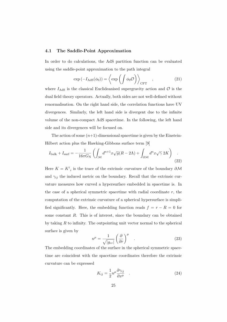
4.1 The Saddle-Point Approximation
In order to do calculations, the AdS partition function can be evaluated
using the saddle-point approximation to the path integral
exp (−IAdS(φ0)) =⟨
exp(∫
φ0O)⟩
CFT
, (21)
where IAdS is the classical Euclideanised supergravity action and O is the
dual field theory operators. Actually, both sides are not well-defined without
renormalisation. On the right hand side, the correlation functions have UV
divergences. Similarly, the left hand side is divergent due to the infinite
volume of the non-compact AdS spacetime. In the following, the left hand
side and its divergences will be focused on.
The action of some (n+1)-dimensional spacetime is given by the Einstein-
Hilbert action plus the Hawking-Gibbons surface term [9]
Ibulk + Isurf = − 116πGN
(∫Mdn+1x
√g(R− 2Λ) +
∫∂M
dnx√γ 2K
).
(22)
Here K = Kii is the trace of the extrinsic curvature of the boundary ∂M
and γij the induced metric on the boundary. Recall that the extrinsic cur-
vature measures how curved a hypersurface embedded in spacetime is. In
the case of a spherical symmetric spacetime with radial coordinate r, the
computation of the extrinsic curvature of a spherical hypersurface is simpli-
fied significantly. Here, the embedding function reads f = r − R = 0 for
some constant R. This is of interest, since the boundary can be obtained
by taking R to infinity. The outpointing unit vector normal to the spherical
surface is given by
nµ =1√|grr|
(∂
∂r
)µ. (23)
The embedding coordinates of the surface in the spherical symmetric space-
time are coincident with the spacetime coordinates therefore the extrinsic
curvature can be expressed
Kij =12nµ∂γij∂xµ
. (24)
25
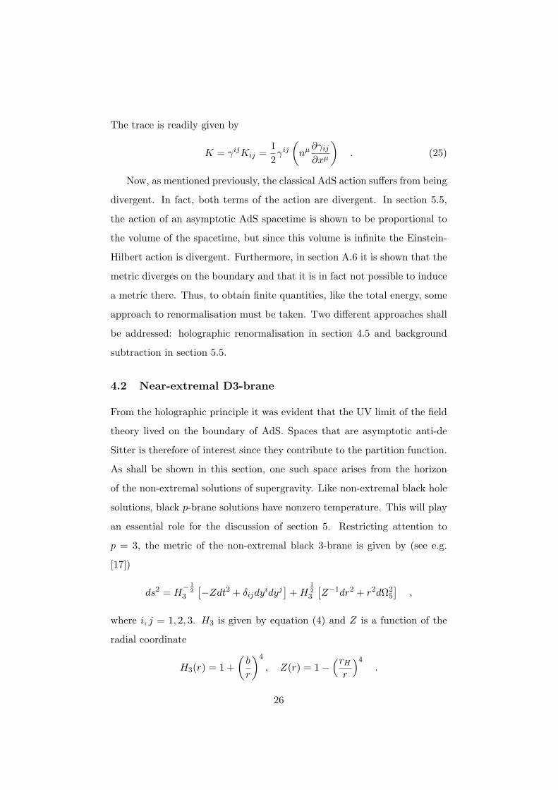
The trace is readily given by
K = γijKij =12γij(nµ∂γij∂xµ
). (25)
Now, as mentioned previously, the classical AdS action suffers from being
divergent. In fact, both terms of the action are divergent. In section 5.5,
the action of an asymptotic AdS spacetime is shown to be proportional to
the volume of the spacetime, but since this volume is infinite the Einstein-
Hilbert action is divergent. Furthermore, in section A.6 it is shown that the
metric diverges on the boundary and that it is in fact not possible to induce
a metric there. Thus, to obtain finite quantities, like the total energy, some
approach to renormalisation must be taken. Two different approaches shall
be addressed: holographic renormalisation in section 4.5 and background
subtraction in section 5.5.
4.2 Near-extremal D3-brane
From the holographic principle it was evident that the UV limit of the field
theory lived on the boundary of AdS. Spaces that are asymptotic anti-de
Sitter is therefore of interest since they contribute to the partition function.
As shall be shown in this section, one such space arises from the horizon
of the non-extremal solutions of supergravity. Like non-extremal black hole
solutions, black p-brane solutions have nonzero temperature. This will play
an essential role for the discussion of section 5. Restricting attention to
p = 3, the metric of the non-extremal black 3-brane is given by (see e.g.
[17])
ds2 = H− 1
23
[−Zdt2 + δijdy
idyj]
+H123
[Z−1dr2 + r2dΩ2
5
],
where i, j = 1, 2, 3. H3 is given by equation (4) and Z is a function of the
radial coordinate
H3(r) = 1 +(b
r
)4
, Z(r) = 1−(rHr
)4.
26

The black brane horizon is located at r = rH . In the extremal case, it was
found that the parameter rp = r3 = b was related by equation (11) to the
combination gsN . This, although not stated, is in fact true for the general
p-brane solution [17]. Thus, using this relation the essential operation is to
take the decoupling limit where the near-horizon decouples from the bulk
gsN 1. This limit of the non-extremal case corresponds to a near-extremal
solution and the harmonic function can be approximated by (13) again(b
`s
)4
∝ gsN 1 ⇒ H3 ≈(b
r
)4
.
One could expect that the limit would have restricted attention to the region
near the horizon and both removed the singularity and the asymptotically
flat region. However, this is not the case as is evident from the form of the
metric
ds2 =r2
b2[−Zdt2 + δijdy
idyj]
+b2
r2Z−1dr2 + b2dΩ2
5 .
The first part is the Schwarzschild-AdS5 black hole metric in local coordi-
nates (Poincare coordinates) where the horizon is R3 instead of S3 while the
second part is the five-sphere as in the extremal case. The metric is asymp-
totic to the anti-de Sitter space and has an inverse temperature β = πb2/rH .
As mentioned in appendix section A.1, the Schwarzschild-AdS metric is, like
the AdS metric, a solution to Einstein’s equations with a negative cosmolog-
ical constant. In order to compare the form here to equation (15), a change
of variables z = b2/r is performed
ds2 =b2
z2
[−Zdt2 + δijdy
idyj + Z−1dz2]
+ b2dΩ25 . (26)
In these coordinates the horizon is located at z0 = b2/rH and the tempera-
ture is β = πz0. The thermodynamical quantities temperature, energy, and
entropy will be given a proper treatment in section 5.
Now, two contributing spacetimes to the partition function have been
identified. The string theory partition function evaluated by the saddle-
27
point approximation given by equation (21) is thus
Zstring ' e−IAdS + e−IBH .
Here, the IBH denotes the action of the Schwarzschild-AdS5 black hole. Sec-
tion 5 will work with this approximation in detail. However, some questions
in relation to classical black holes in flat space are worth mentioning. Most
of the classical work done on black holes assumes asymptotic flatness, sta-
tionarity, and other various things reviewed in section D.5. The theorems
developed therefore rely upon such assumptions. Addressing black holes
in asymptotic anti-de Sitter space naturally rises questions about theorems
of uniqueness, positive mass, initial values, etc. (some of these questions
are addressed in [20] and [31]) In addition, section D contains a complete
macroscopic description of the thermodynamic analogy of four dimensional
black holes in asymptotic flat space. The results of black hole thermodynam-
ics are here directly extended to the discussion of their higher dimensional
generalisations.
4.3 Global Coordinates
In sections 2.1 and 4.2, the two geometries of the black Dp-branes have been
derived in Poincare coordinates given by equation (15) and (26), respectively.
These coordinates only cover a part of the manifold, but one could also
consider global covering coordinates. Appendix A contains among other
things a discussion of different coordinate choices for anti-de Sitter space.
In particular, mappings between them are presented. In this section, the
two metrics given in global coordinates by equation (59) are generalised to
d = n+ 1 spacetime dimensions, that is
ds2 = −V dt2 + V −1dr2 + r2dΩ2n−1 , (27)
28

where dΩ2n−1 is the metric of a (n − 1)-dimensional unit sphere Sn−1. The
covering space of anti-de Sitter space is given with the static form
V (r) = 1 +r2
b2, (28)
where the radius of curvature is denoted by b. The period of the associated
imaginary time coordinate is arbitrary for the metric stated. However, a
constraint is later required in order to relate it to the Schwarzschild black
hole solution which can be introduced in anti-de Sitter space by
V (r) = 1 +r2
b2− r2
0
rn−2= 1 +
r2
b2− wnM
rn−2
wn =16πGN
(n− 1)Vol(Sn−1), (29)
where r0 was the term encountered for the Schwarzschild black hole in flat
space in equation (8) and is here used to define wn such that M is the
mass of the black hole as shown later. GN denote the (n + 1)-dimensional
Newton’s constant and Vol(Sn−1) the (n − 1)-spherical surface area of the
corresponding unit sphere. Note that the function V given by (29) tends
asymptotically towards that of anti-de Sitter space given by (28) as r tends
to infinity.
4.4 The Conformal Boundary
Section A.6 shows that AdS evaluated on the boundary has a second order
singularity. For this reason it is necessary to pick a positive function f ,
called the defining function, such that
g(0) = f2g|∂M
constitutes an induced metric on the boundary. For equation (71), which is
the metric for a hypersurface of constant radial coordinate of the metric by
equation (29), a natural choice could be f = b/r, for example. This proce-
dure, which can be done for any asymptotic AdS space, defines a conformal
29
structure. The metric g(0) depends, however, on the choice of f and different
choices are related by a conformal transformation f ′ = feu.
A natural metric for dual field theory in the UV is obtained by removing
the conformal factor r2/b2 making the above choice of f . This gives a
conformal structure in global coordinates of R × Sn−1. Correspondingly,
the choice f = z/w for the defining function in local coordinates given by
equation (14) leads to the conformal boundary R × Rn−1. Thus, in some
sense the physics looks like it depends on the choice of coordinates, but
by the choice of coordinates the definition of the Hamiltonian will also be
affected and the physics is, as expected, in fact the same. Since the radial
coordinate plays the role of an energy scale in the gauge theory, the choice of
coordinates can also be seen as a choice of regulator at that energy scale [17].
This shall be evident from the treatment of holographic renormalisation in
section 4.5.
One can show that the two boundaries of local and global coordinates are
conformally related in their Euclideanised versions. Removing the conformal
factor in equation (15) using the above choice of the defining function, the
boundary takes the following form
ds2 = ηµνdxµdxν .
Now considering the Euclideanised version of the metric ηµν → δµν and
writing the Euclideanised space in polar form
δµνdxµdxν = dx2 + r2dΩ2
n−1 .
Introducing the coordinate x = ln τ one has dx2 = r2dτ2, thus
dx2 + r2dΩ23 = x2(dτ2 + dΩ2
3) .
This is exactly the form of the boundary in the global coordinates given by
equation (69) times the conformal factor x2. This can be seen by setting
the coordinate τ equal to it.
30

4.5 Holographic Renormalisation
In this text, the primary method applied in detail when determining thermo-
dynamical quantities related to asymptotic AdS spaces will be background
subtraction, following Witten [30]. However, it is worth considering a dif-
ferent approach known as holographic renormalisation. This is a quite far-
reaching approach and has a natural interpretation in the dual field theory.
The essential key points needed to obtain the stress-energy tensor will be
addressed in this section. For more information, see [25], [6], [2].
From the discussion of section 3.3 and 3.4 and the findings of section 4.2,
asymptotic AdS spacetime solutions to Einstein’s equations with a negative
cosmological constant are of natural interest. Given some representative of
the conformal structure as defined in section 4.4, it can be shown that one
can obtain a solution of Einstein’s equations which is asymptotic AdS [25].
The metric in the neighbourhood of the boundary z → 0 takes the form
ds2 =b2
z2
(dz2 + gij(x, z)dxidxj
)gij(x, z) = g(0)ij + zg(1)ij + z2g(2)ij + ... .
Einstein’s equations can be solved order by order in z to determine the
coefficients g(k)ij for k > 0. All the coefficients can be determined uniquely
in terms of g(0). It turns out that all coefficients in odd powers of z vanish
up to order zn. Notice that choosing g(0)ij = δij with all other coefficients
zero reduces the solution to the AdS metric given in Poincare coordinates by
equation (15). To simplify computation, one can introduce the coordinate
ρ = z2
ds2 = gµνdxµdxν = b2
(dρ2
4ρ2+
1ρgij(x, ρ)dxidxj
)gij(x, ρ) = g(0) + ...+ ρ
d2 g(d) + h(d)ρ
d2 log ρ+O(ρ
d+12 ) . (30)
Any asymptotic AdS metric can be brought into this form near the boundary,
which is located at ρ = 0. The logarithmic coefficient h(d) is only non-zero
31

when n is even. If the bulk metric is conformally flat, an exact solution to
Einstein’s equations exists and is given by [24]
gij(x, ρ) = g(0) + g(2)ρ+ g(4)ρ2
g(2)ij =1
n− 2
(Rij −
R2(n− 1)
g(0)ij
)g(4)ij =
14
(g(2))2ij =
14g(2)ip g
pq(0) g(2)qj , (31)
where the curvatures R and Rij are given by the metric g(0).
Now that an expansion for the solution of an asymptotic AdS spacetime
is given, the corresponding action given by equation (22) can be addressed.
It is evident that both integrals are divergent; the bulk action is proportional
to the infinite volume of spacetime while the surface term diverges since the
induced boundary diverges at the boundary. To render the action finite,
one must perform a renormalisation scheme. First step is to introduce a
regularisation procedure. This is done by introducing a regulator (or cutoff)
ε on the radial coordinate such that the bulk action is evaluated for ρ ≥ ε
(recall that the boundary is at ρ = 0) and the surface term at ρ = ε.
Using the asymptotic solution given by (30), one can evaluate the regularised
action as a power series of ε [24]. Restricting to n = 4, the regularised action
is
Ireg =1
16πGN
∫dnx
√g(0)
(ε−2a(0) + ε−1a(2) − log εa(4)
)+O(ε0) . (32)
The regularisation scale ε can be thought of as specifying a spatial hyper-
surface a finite amount within the interior of spacetime. Interestingly, in
addition to the terms addressed below, one finds a logarithmic divergence.
For n = 4 it takes the value [15]
a(4) log ε = b3(
18RijRij −
R2
24
)log ε .
Note that this vanishes for a flat background. To make the action finite,
one can perform a minimal subtraction; that is, to subtract the pieces that
32
divergence as one goes to the boundary by the corresponding counter terms.
These terms are a finite set of boundary integrals, which only depend, like
the coefficients given in equation (30), on the induced conformal structure
at the boundary g(0). Including the counter terms, the renormalised action
is written
Iren[g(0)] = limε→0
(Ireg[g(0), ε] + Ict[g(0), ε]
).
Only two counter terms and the additional logarithmic one are needed to
cancel all divergences for the case of n = 4. They take the form [17]
Ict[g(0), ε] =1
16πGN
∫ρ=ε
dnx√−γ[
6b
+b
2R− a(4) log ε
]. (33)
The metric γij is the metric on the boundary induced by restricting ρ to be
the constant ε. Note that the same metric was also used in the surface term
to compute the form given by equation (32). The R and Rij are the Ricci
scalar and Ricci tensor for the metric γij , respectively.
From this point of view, it is now possible to understand the discussion
given in section 4.4 of why the choice of coordinates (or, more precisely,
the choice of conformal boundary structure) seems to affect the physics.
The counter terms are given by the coefficients g(2), ..., g(n−2), which are
uniquely determined on the choice of g(0). g(0) is, however, only determined
up to a conformal transformation, and since the logarithmic divergence is
regularisation independent the action depends on the choice of conformal
boundary structure g(0) [15]
I[eug(0)] = I[g(0)] +A[g(0), u] .
This anomalous transformation is known as the holographic Weyl anomaly
and is only present for odd spacetime dimensions. Although the anomaly
may vanish in one background, its metric variation may not. The stress-
energy tensor can therefore have a contribution from the anomalous varia-
tion, which is the case for AdS in global coordinates. In the following, the
logarithmic term will be neglected.
33
The stress-energy tensor at the boundary can be extracted from the
renormalised action in the following way
Tij =2√−g(0)
δIren
δgij(0)
.
One can evaluate this expression by first computing the stress-energy tensor
at a finite distance within the interior (that is in the regulated theory) and
thereafter go to the boundary (removing the regulator)
Tij = limε→0
2√−g(x, ε)
δIren
δgij(x, ε)= lim
ε→0
1ε
n2−1
1√−γ
δIren
δγij.
This way, one can express the stress-energy tensor in terms of the induced
metric γij
Tij [γ] = T reg[γ] + T ct[γ], T reg[γ] =1
8πGN(Kij −Kγij) ,
where the regulated contribution comes from the regulated action and Kij
and K is the extrinsic curvature and its trace as defined in equation (24)
and (25). The counter term contribution is calculated from the boundary
integrals given by equation (33). The second counter term is proportional
to an Einstein-Hilbert action and thus the finite stress-energy tensor in the
case of n = 4 is [2]
Tij [γ] =1
8πGN
(Kij −Kγij +
3bγij +
b
2
[Rij −
12Rγij
]). (34)
Using this formula the stress-energy tensor can be determined for the
AdS5 metric given in local coordinates by equation (14). The outpoint
normal vector is given by equation (23)
nµ =r
b
(∂
∂r
)µ.
The extrinsic curvature of the boundary and its trace is
K00 = −r2
b3, K11 = K22 = K33 =
r2
b3, K = γijKij =
2b
.
34
Evaluating the stress-energy tensor by equation (34) it is thus found to
vanish. In fact the first counter term is enough to cancel all divergences.
A zero stress tensor is to be expected for an empty space, but as shall be
shown this depends on the choice of conformal boundary structure.
It has been shown in [24] that one can express the stress-energy tensor
in terms of the expansion coefficients of gij given by equation (30) as
Tij =nb
16πGN
(g(d)ij +X
(d)ij
), (35)
where X(d) depends on the number of dimensions. For odd d, this contri-
bution vanishes. For the case of n = 4, which is related to asymptotic AdS5
spacetimes, one has [6]
X(4)ij = −1
8g(0)ij
[(Tr g(2))
2 − Tr g2(2)
]− 1
2(g2
(2))ij +14g(2)ijTr g(2)
(g(2))2ij = g(2)ip g
pq(0) g(2)qj
Tr g(2) = gij(0)g(2)ij
Tr g2(2) = gij(0) g(2)ip g
pq(0) g(2)qj . (36)
Using this prescription the stress-energy tensor of the boundary of the
conformally flat AdS5 can be determined. The metric is given in global co-
ordinates by equation (27). It can be brought to the form given by equation
(31) by the following coordinate transformation (also used in section A.3)
r2
b2=
1ρ
(1− ρ
4
)2and t2 = b2(x0)2 .
Choosing the metric gS3 = diag(1, sin2 ψ, sin2 ψ sin2 φ) for the unit three-
sphere, the metric coefficients g(0), g(2) and g(4) can be read off to be
g(0)ij = diag(−1, 1, sin2 ψ, sin2 ψ sin2 φ)
g(2)ij = −12
diag(1, 1, sin2 ψ, sin2 ψ sin2 φ)
g(4)ij =116g(0)ij . (37)
35
Using equation (36), one finds X(4)ij = 1
4δi,0δj,0. Scaling the coefficients by
1/b2 to get the stress-energy tensor in ordinary units, this result together
with (35) yields
Tij =1
64πGNb(4δi,0δj,0 + g(0)ij
).
For the case of global coordinates where the boundary structure is R× S3,
the field theory is living on S3. To obtain the total energy, one integrates
over the three-sphere, with volume 2π2b3, thus obtaining
E =3πb2
32G(5)N
.
Although a non-zero energy for a vacuum solution might seem odd in relation
to what was found for the choice of local coordinates, it is expected from the
previous discussion and matches the Casimir energy of the free field theory
limit [17], [2]. As was shown in section 4.3, it is possible by performing a
conformal transformation to bring the choice of g(0) on a conformally flat
form. This is the case treated above in Poincare coordinates where g(0)
is flat. The stress-energy tensor vanishes and the total energy of the field
theory on R3 is zero. The energy thus depends on the choice of g(0) and can
be understood as a constant shift in energy.
For the black hole solution given by equation (29) the same method
can be applied. Since the metric is asymptotic AdS, it is possible to put
it on the form given by equation (30) performing the following coordinate
transformation
r2
b2=
1ρ
(1− ρ
4
)2+
r20
4b2ρand t2 = b2(x0)2 .
Expanding in terms of ρ to second order reveals that g(0) and g(2) is given
by equation (37) while g(4) takes the form
g(4)ij =116
diag(
12r20 − b2
b2, (b2 + 4r2
0)gS3
).
36
Again, one finds X(4)ij = 1
4δi,0δj,0, but the form of g(4)ij yields an additional
term to the total energy of the black hole metric
E =3πb2
32G(5)N
+3πr2
0
8G(5)N
.
The first term is exactly what was obtained above for AdS5 and the energy
correctly reduces in the case of r0 = 0. Letting r20 = w4M and using the
expression (39), the second term is seen to be in agreement with the result
obtained using the method of background subtraction given by equation
(49). In [2] and [17] the stress-energy tensor has been determined using
equation (34).
37
5 Thermal Phase Transition in Anti-de Sitter Space
As mentioned in section 4.1, the saddle-point approximation will be used
to evaluate the path integral. In appendix C.1, the connection between the
Euclidean path integral formulation and the canonical statistical ensemble
is established. It is shown that a partition function can be formed by an
integral over metrics; that is, the assumption that the dominant contribution
to the path integral comes from the background fields that extremize the
action. The action introduced in equation (22) is therefore of interest.
In this section, the connection is utilised to study the thermodynamical
properties of the asymptotic anti-de Sitter backgrounds. Referring to equa-
tion (79), the two contributing metrics are the anti-de Sitter space metric
and the Schwarzschild-anti-de Sitter metric, respectively. The Euclideanised
versions of these metrics are non-singular positive-definite solutions satisfy-
ing the required periodic thermal boundary conditions [14], [30]. It will be
possible to answer questions of whether one can have a quantum field theory
at a finite temperature by considering the thermodynamical stability of the
black hole solution. This is readily given by the specific heat. However, the
black hole configuration must also be favourable over pure thermal radia-
tion in anti-de Sitter space; that is, have dominant negative free energy. The
implication on the dual field theory living on the boundary of the anti-de
Sitter space will be discussed.
In section 4.3, global coordinates of the two contributing metrics were
introduced and these shall be used exclusively in the following. Throughout
the section, the general (n + 1)-dimensional case will be considered, where
n is the number of spatial dimensions. Specific examples are, however,
dedicated to the cases of n = 3 and n = 4, which are of particular interest.
The former was considered by Hawking and Page [14] and the latter is the
case considered in the near-horizon and decoupling limit of the D3-brane
geometry.
38

5.1 Criterion for Confinement/Deconfinement
As mentioned above and from the discussion of the holographic principle, the
string theory on the asymptotic AdS5 backgrounds is related to a strongly
coupled conformal field theory living on the boundary R × S3. In the case
of the Schwarzschild-AdS solution, this corresponds to having a dual field
theory at a finite temperature. However, a temperature introduces a energy
scale in the theory which therefore breaks conformal symmetry. When using
the Euclidean approach to quantum gravity the metrics are Euclideanised
and the boundary structure changes accordingly to S1×S3. This is thus the
appropriate structure to consider a field theory on S3 with finite temperature
where supersymmetry-breaking boundary conditions has been imposed in
the S1 direction. In the following, attention is restricted to the N = 4
theory on this finite volume manifold.
A criterion for whether the field theory in question is in a confining
phase or a de-confining phase is of interest. This will quantify whether a
phase transition occurs in the strongly coupled theory or not at large N .
A criterion in finite volume for confinement is whether the free energy is
of order O(1) or of order N2. When the theory is confining, the order of
O(1) shows that the contribution is the color singlet hadrons, and when it
is deconfining, the order of N2 shows that the contribution is the gauge
fields, i.e. the gluons. The N = 4 theory on S1 × S3 in the large N limit is
expected to have a low temperature phase with a free energy of order O(1)
and a high temperature phase with a free energy of order N2 (see [29]).
5.2 Schwarzschild Black Hole in Anti-de Sitter Space
To determine the temperature of the black hole, one requires that the metric
does not exhibit a conical singularity at the horizon. In section 5.3, this is
done in detail, but requires an expanding around the horizon. It must there-
fore be ensured that a positive root actually exists before the temperature
39
can be determined. The horizons are given by the roots of the gravitational
potential V (r) given in equation (29)
1 +r2
b2− wnM
rn−2= 0 . (38)
The largest positive root r+ of this equation is the black hole event horizon.
It is evident from Decartes’ sign rule that there is at most one positive
root. This, if it exists, must therefore be r+. This quantity determines
the euclidean section, since the positive-definiteness of the metric is only
maintained by restricting the radial coordinate to the region r ≥ r+. In
addition, the largest root also defines the mass M of the black hole
M =rn−2
+
wn
(1 +
r2+
b2
), (39)
where the constant wn, given by equation (29), is chosen such that M is in
fact the mass. This will also be evident from the computation of the energy
given in section 5.6. In the following, the roots for the case of n = 3 and
n = 4 are considered.
The Schwarzschild-anti-de Sitter metric in four dimensions has a classical
interest and is presented in some details in appendix A by equation (59). It
is, of course, the same as in equation (27) with n = 3. For this particular
case, w3 = 2GN and Vol(S2) = 4π, therefore the function V takes the form
V (r) = 1 +r2
b2− 2MGN
r. (40)
The event horizon is found for a suitable r = r+ satisfying the equation
V (r+) = 0. Hence, a cubic equation is given
r3+ + b2r+ − 2MGNb
2 = 0 ,
where the real coefficients are given by a1 = 0, a2 = b2 and a3 = −2MGNb2.
40
The discriminant D of a cubic equation is given as
D = Q3 +R2
Q =3a2 − a2
1
9=a2
3> 0
R =9a1a2 − 27a3 − 2a3
1
54= −27a3
54> 0 .
Hence D > 0 which means the cubic equation has two imaginary roots and
one real root, say r+. The real root is given by
r+ = S + T − 13a1 = S + T
S =(R+√D) 1
3> 0
T =(R−√D) 1
3.
This can be seen since S − T is always real leaving the two other roots
imaginary. However, the real root should be positive in order to make sense
physically. The requirement S + T > 0 is equal to R being positive. Hence,
there always exists one event horizon in the n = 3 Schwarzschild-anti-de
Sitter space given by a real positive root.
In the case of five dimensional anti-de Sitter space one has Vol(S3) = 2π2
and w4 = 8GN/3π. The function V takes the form
V (r) = 1 +r2
b2− 8GN
3πM
r2.
Using r0 = w4M and solving for the roots of the quartic equation V (r+) = 0
r4+ + b2r2
+ − r0b2 = 0 .
For this particular form, one can solve for r2+
r2+ =
b2
2
(±√
1 +4r2
0
b2− 1
).
The argument of the square root is greater than one. The term in the
parenthesis is therefore positive for the positive sign and negative for the
41
negative sign. Solving for r+, one therefore finds that the equation has a
conjugate imaginary pair of roots and two real roots of equal magnitude,
but opposite sign. The positive real root is given by
r+ =
√√√√b2
2
(√1 +
4r20
b2− 1
).
Hence, there exists only one event horizon in the case of n = 4 for the
Schwarzschild-anti-de Sitter space.
5.3 The Periodicity of Imaginary Time
With the existence of an event horizon it is now possible to turn to determin-
ing the temperature. Unlike some spaces, AdS has no natural temperature
associated with it. One must impose a periodicity in the imaginary time
to construct thermal states, say β. The inverse temperature is thereby de-
termined by the periodicity of imaginary time β = T−1. Rotating the time
coordinate into the imaginary plane by τ = it, one can identify the sec-
tion for which the metric is positive-definite. This section is given by the
constraint r ≥ r+ on the radial coordinate, where r+ is the largest root of
equation (38). For the case of n = 3 and n = 4 it was shown that one
positive real root always exists.
The geometry of an Euclideanised Schwarzschild-AdS black hole solution
has a conical part. To see this, consider the geometry of a cone which is
readily described in terms of a flat space metric in polar coordinates (ρ, θ)
ds2 = dρ2 + ρ2dθ2 (41)
with the angular coordinate having a domain of θ ∈ [0, 2π −∆] such that a
piece of the plane is missing for ∆ 6= 0. For a non-zero choice of ∆, the origin
of the plane ρ = 0 is singular. Such a conical singularity is not desired if the
metric is to describe a black hole where the horizon is non-singular. One
must require that the horizon is non-singular even though there can not be
42
a continuation inside the horizon. Hence, the periodicity of the imaginary
time is constrained by ∆ = 0.
To identify the correct periodicity of the Schwarzschild-AdS solution,
consider the expansion of the coefficient V (r) around the horizon r = r+ to
first order
V (r) ≈
[2r+ + wnM(n− 2)b2r1−n
+
b2
]r
=[nr2
+ + b2(n− 2)b2r+
]r ,
where the horizon is shifted to zero by defining the coordinate r = r − r+.
Note that the zeroth order vanishes due to the defining property V (r+) = 0.
The second equality is obtained by using the mass of the black hole in terms
of the horizon given by equation (39). Now, defining ρ =√r, the metric
shows a conical form
ds2 ≈ 4V −1
(dρ2 +
ρ2
4
[nr2
+ + b2(n− 2)b2r+
]2
dτ2
)+ r2
+dΩ2n−1 .
Denoting the period of τ by β, the condition for a smooth non-singular space
gives12
[nr2
+ + b2(n− 2)b2r+
]β = 2π .
Hence, the periodicity of the imaginary time is obtained as a function of the
black hole radius r+
β =4πb2r+
nr2+ + b2(n− 2)
, (42)
for which the temperature of the the black hole is given T = β−1. It is
interesting to see how the temperature behaves in different limits of r+. For
a small black hole r+ b
β ' 4πr+
n− 2,
the temperature is large and for a black hole with large radius r+ b
β ' 4πb2
nr+, (43)
the limit shows that the temperature scales with the black hole’s size.
43
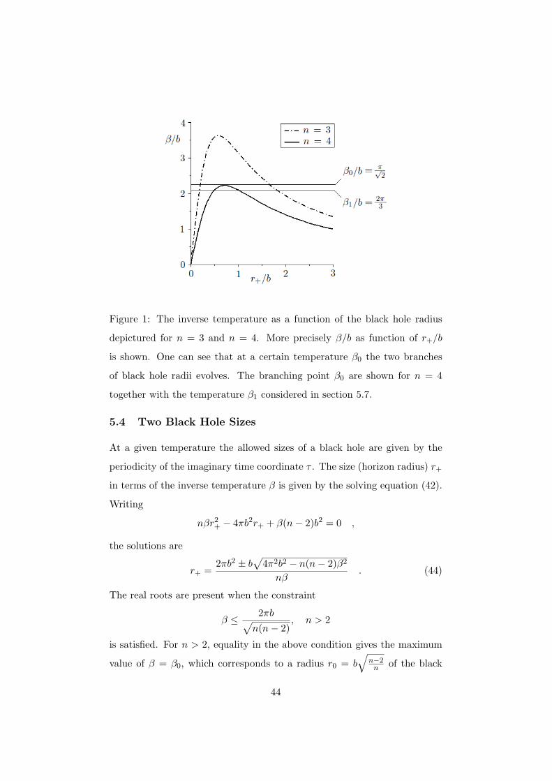
Figure 1: The inverse temperature as a function of the black hole radius
depictured for n = 3 and n = 4. More precisely β/b as function of r+/b
is shown. One can see that at a certain temperature β0 the two branches
of black hole radii evolves. The branching point β0 are shown for n = 4
together with the temperature β1 considered in section 5.7.
5.4 Two Black Hole Sizes
At a given temperature the allowed sizes of a black hole are given by the
periodicity of the imaginary time coordinate τ . The size (horizon radius) r+
in terms of the inverse temperature β is given by the solving equation (42).
Writing
nβr2+ − 4πb2r+ + β(n− 2)b2 = 0 ,
the solutions are
r+ =2πb2 ± b
√4π2b2 − n(n− 2)β2
nβ. (44)
The real roots are present when the constraint
β ≤ 2πb√n(n− 2)
, n > 2
is satisfied. For n > 2, equality in the above condition gives the maximum
value of β = β0, which corresponds to a radius r0 = b√
n−2n of the black
44

hole. This shows that there exists a minimum value of the temperature
T0 = β−10 , which initiate two possible black hole radii. At finite temperature
above T0 there are always two valid solutions and the positive branch always
has greater radius than the negative branch. The radius of the black hole
is therefore a multivalued function of the inverse temperature. The two
branches are illustrated for n = 3 and n = 4 in figure (1). For n = 2,
there is always two real roots: zero and 2πb2/β while for n < 2 there are no
positive real roots when the temperature is real and positive.
5.5 Actions and Partition Functions
Other interesting thermodynamical quantities can be obtained by consider-
ing the Euclideanised action. The two metrics given by equation (28) and
(29) both extremize the Euclidean action. Keeping the normalisation of the
cosmological constant introduced in equation (60), the action given by equa-
tion (22) of the maximally symmetric spaces are seen to be proportional to
the volume of spacetime
I = − 116πGN
∫dn+1x
√g [R− 2Λ]
= − 116πGN
∫dn+1x
√g
[−n(n+ 1)
b2+n(n− 1)
b2
]=
n
8πGNb2
∫dn+1x
√g .
The action has additional surface terms, but for the Schwarzschild-AdS they
vanish because the black hole correction in equation (29) vanishes too quickly
when approaching the boundary. Since both the anti-de Sitter space and the
black hole spacetime have infinite volume, one considers the finite difference
between the two actions. The black hole is thus compared to the empty
AdS space. This operation can be performed by introducing a regularisation
45
cutoff R for the radial coordinate r
VAdS =∫ β′
0dτ
∫ R
0
∫Sn−1
rn−1dΩ =β′Vol(Sn−1)
nRn
VBH =∫ β
0dτ
∫ R
r+
∫Sn−1
rn−1dΩ =βVol(Sn−1)
n
[Rn − rn+
].
However, in order to compare the two volume integrals, one must make sure
they describe the same AdS space asymptotically r → ∞. The black hole
solution has a fixed period β given by equation (42) while the anti-de Sitter
solution can have an arbitrary period β′. To make a comparison between
the two volumes, one must therefore require that the period β′ is adjusted
such that the geometry of the two spaces equals at the cutoff hypersurface
r = R. Considering the two metrics at fixed r = R given by equation (27)
with V defined by (28) and (29), respectively, one sees that only the time
component introduces a difference in the volume since the sphere part is
identical. This implies that the two periods β and β′ are related by
limr=R
∫dn+1x
√gBH = lim
r=R
∫dn+1x
√gAdS∫ β
0dτ
√1 +
R2
b2− wnM
Rn−2=
∫ β′
0dτ
√1 +
R2
b2
β
√1 +
R2
b2− wnM
Rn−2= β′
√1 +
R2
b2,
where M is a function of r+ given by equation (39). The period β′ can
be expressed in terms of β and approximated in the limit of the cutoff R
tending to infinity
β′ = β
√1− wnMb2
Rn + b2Rn−2
≈ β
[1− 1
2wnMb2
Rn
]= β
[1− 1
2
(1 +
r2+
b2
)rn−2
+ b2
Rn
].
46
Note that for large R, the expansion of the square root is valid. Using the
large R limit of β′ the action difference becomes
I =n
8πGNb2limR→∞
(VBH(R)− VAdS(R))
=βVol(Sn−1)
8πGNb2
([Rn − rn+
]−[Rn − 1
2(rn−2
+ b2 + rn+)])
=βVol(Sn−1)16πGNb2
(rn−2
+ b2 − rn+)
.
Inserting the inverse temperature β given by (42), the action difference is
I =Vol(Sn−1)
4GN
[b2rn−1
+ − rn+1+
nr2+ + (n− 2)b2
]. (45)
The partition function of the black hole solution is
−I = logZBH − logZAdS = logZBH
ZAdS,
and the free energy
FBH − FAdS = − 1β
[logZBH − logZAdS]
=Vol(Sn−1)16πb2GN
[b2rn−2
+ − rn+]
. (46)
A phase transition becomes possible if the free energy goes from positive
to negative; that is, a transition from empty space to a black hole. This is
exactly what happens. For sufficiently small r+ the free energy is positive
and for sufficiently large r+ it is negative for all values of n. However, for
this black hole configuration to be stable the heat capacity will have to be
positive. The heat capacity is considered in the next section.
In relation to section 5.4 where it was found that at a given temperature
two possible radii of the black hole could occur, it is evident from the free
energy that the large radius always will be more favourable than the small
radius. In fact, the small radius always has positive free energy, which
means that it is less probable than empty space, as will be shown in the
next section.
47
5.6 Energy, Specific Heat Capacity
From the temperature it was possible to match the period of AdS space
to that of the Schwarzschild-AdS black hole at infinity and thus determine
the action difference. Given the action difference and thereby the parti-
tion function, the free energy was given. It is possible to determine other
thermodynamical quantities as well: the average energy, the specific heat,
and the entropy. The energy allows a consistency check of the mass M de-
fined by equation (39) and the specific heat capacity to be calculated. The
heat capacity will answer the question about stability of the two black hole
configurations. The entropy shall be considered in section 5.8.
From appendix C.1, the average energy is given by
〈E〉 =∂I
∂β=∂I
∂r
∂r
∂β=∂I
∂r
(∂β
∂r
)−1
.
The action is given by equation (45) in terms of the location of the horizon
r+, which is a multivalued function of the inverse temperature. There are
two points to note about the above expression of the energy. First, since
β is a function of r+, the energy should also be a function of r+. One
should not be confused that there are two consistent radii of black holes at a
given temperature. Second, expressing the energy as above, mathematically
speaking, the energy is not well-defined at the branching point r0 of the two
radii solutions, since the derivative of the inverse temperature will be zero.
However, physically, the energy is expected to be defined and finite at r0.
To perform the calculation, it is helpful to start by using the form of the
denominator to substitute the function β in
I =Vol(Sn−1)
4GN
β
4πb2[b2rn−2
+ − rn+]
.
Defining γ = Vol(Sn−1)/(16πGNb2), the derivative is
∂I
∂β= γ
(b2rn−2
+ − rn+)
+ γ((n− 2)b2rn−3
+ − nrn−1+
)β∂r+
∂β. (47)
48
Making the arbitrary choice of focusing on the branch of r+ > r0, which is
given by choosing the positive sign in equation (44), the partial derivative
with respect to β is
∂r+
∂β= −(n− 2)b√
D− 2πb2 + b
√D
β2n,
where D = 4π2b2 − β2(n− 2)n is the determinant. Noting that the second
part of the above expression contains r+/β the following combination can
be written as
β∂r+
∂β= r+
[nr2
+ + (n− 2)b2
(n− 2)b2 − nr2+
]. (48)
Substituting this
∂I
∂β= γ
(b2rn−2
+ − rn+)
+ γrn−2+
(nr2
+ + (n− 2)b2)
= γ(n− 1)[rn+ + b2rn−2
+
].
An expression for the energy in terms of the horizon is thus obtained
〈E〉 =(n− 1)Vol(Sn−1)
16πGN
[b−2rn+ + rn−2
+
]= M . (49)
As indicated, this corresponds exactly to the definition of the black hole
mass given in equation (39) with the choice of wn. The energy is seen as
expected to be positive for r ≥ 0 for all n, which also means that it is finite
at r0.
It is now possible to compute the specific heat and address the question
about the stability of the black hole configuration
CV = −β2∂〈E〉∂β
= −γ(n− 1)[nrn−1
+ + b2(n− 2)rn−3+
]β2∂r+
∂β.
Using the result from equation (48)
β2∂r+
∂β=
4πb2r2+
(n− 2)b2 − nr2+
.
The specific heat capacity is obtained in terms of the horizon radius
CV =(n− 1)Vol(Sn−1)
4GN
[nrn+1
+ + b2(n− 2)rn−1+
nr2+ − (n− 2)b2
]. (50)
49

When the dominator is zero, the function goes from negative to positive.
At this point, which was already encountered in section 5.4, namely r0 =
b√
n−2n , a bifurcation happens. The result shows that the branch for which
the black hole radius r+ is greater than r0 always has positive specific heat.
While, the branch for which the radius r+ is lesser than r0 always has nega-
tive specific heat. The larger radius is therefore always a thermodynamical
stable configuration, but need not always be the most favourable.
Since the branch of black hole radii larger than r0 is always a stable
configuration it is of interest to see if there is a temperature for such radii
at which the free energy becomes negative. At such a temperature, the
black hole configuration will be more probable than pure thermal radiation
in an AdS background. By restricting attention to the solution given by
equation (44) with positive sign, the radius can be considered a function of
β. Substituting r+(β) into the free energy given by equation (46) one finds
that the free energy is zero at
β1 = ± 2πbn− 1
. (51)
In section 5.4, it was shown that an event horizon existed for n ≥ 2. As-
suming this and discarding the negative solution of β1, the derivative of the
free energy evaluated at β1 is
∂F
∂β
∣∣∣∣β=β1
=Vol(Sn−1)(n− 1)2bn−3
16π2GN, n ≥ 2 , (52)
which is seen to be positive. The free energy therefore changes sign from
positive to negative for decreasing values of β. Thus, the black hole will
be energetically favourable when the temperature is greater than T1 = β−11 .
The corresponding radius of the black hole is independent of n and is r1 = b.
When n > 2, one can check for consistency that β1 ≤ β0 or equivalent
T0 ≤ T1; that is, the black hole solution becomes stable and favourable at
a higher temperature than the branching temperature T0. One obtains the
50

relationn2 − 2n
n2 − 2n+ 1≤ 1, n > 2 ,
which is always true, although the difference |β1 − β0| becomes smaller and
smaller as the spatial dimensions n increases.
5.7 Phase Transition
This section summaries the findings of the previous sections about the phase
transition as a function of temperature. It should be mentioned that the
cases of n = 3 and n = 4 are completely similar to the general case. Table
(1) shows specific values of the aforementioned specific points of events.
n β0 r0 β1 r1
3 2πb√3
b√3
πb b
4 πb√2
b√2
2πb3 b
...
n 2πb√n(n−2)
b√
n−2n
2πbn−1 b
Table 1: Particular values of the bifurcation temperature β0 and phase
transition temperature β1 for the cases of n = 3, n = 4, and the general
case. The temperature is given by T = β−1. Note that r1 > r0 and β1 < β0.
For temperatures lower than T0, the only equilibrium which is possible is
thermal radiation in anti-de Sitter space. When the temperature reaches T0,
there are, in addition to the pure thermal radiation, two possible black holes.
Only the larger of them has positive specific heat as was shown from equation
(50). Using equation (44), the free energy given by (46) can be expressed in
terms of β for the small radius and the large radius, respectively. For the
larger black hole, the free energy has a positive root at β1 given by equation
(51). Looking at the derivative of the free energy at the point β1 given by
equation (52), one finds that the free energy goes from positive to negative
with decreasing β.
51
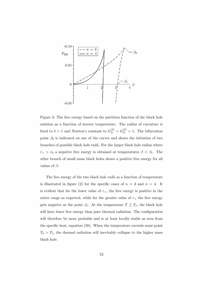
Figure 2: The free energy based on the partition function of the black hole
solution as a function of inverse temperature. The radius of curvature is
fixed to b = 1 and Newton’s constant to G(4)N = G
(5)N = 1. The bifurcation
point β0 is indicated on one of the curves and shows the initiation of two
branches of possible black hole radii. For the larger black hole radius where
r+ > r0 a negative free energy is obtained at temperatures β < β1. The
other branch of small mass black holes shows a positive free energy for all
values of β.
The free energy of the two black hole radii as a function of temperature
is illustrated in figure (2) for the specific cases of n = 3 and n = 4. It
is evident that for the lower value of r+, the free energy is positive in the
entire range as expected, while for the greater value of r+ the free energy
gets negative at the point β1. At the temperature T & T1, the black hole
will have lower free energy than pure thermal radiation. The configuration
will therefore be more probable and is at least locally stable as seen from
the specific heat, equation (50). When the temperature exceeds some point
T2 > T1, the thermal radiation will inevitably collapse to the higher mass
black hole.
52
5.8 Entropy and Field Theory
Using the expression for the average energy (49), the entropy is readily given
in terms of the location of the event horizon r+
SBH = β〈E〉 − I =Vol(Sn−1)
4GNrn−1
+ . (53)
An important thing to note is that since the surface at r+ is the area of
the horizon A = Vol(Sn−1)rn−1+ , the Hawking-Bekenstein formula for the
entropy is satisfied
SBH =A
4GN.
The entropy of the black hole can be compared to the predictions for the
field theory taken to be on the boundary in the sense explained in section
3.4. As mentioned in section 5.1, the boundary manifold of the asymptotic
AdSn spaces is Sn−1×S1. The system on Sn−1 will be at high temperatures
as β → 0. As is evident from equation (42), the limit of β → 0 can be
taken two ways; either r+ → 0 or r+ → ∞. From the previous discussion,
it is apparent that large r+ is the most favourable configuration. This also
means that the mass of the black hole is taken to be large. The limit given
by equation (43) is therefore valid.
With this knowledge, one can express the entropy for the large black
hole in quantities related to the field theory. It should be noted that this
result is only valid for large effective coupling gsN 1. Restricting to the
case of n = 4 and using the five dimensional Newton’s constant given on the
form (3.3), it becomes possible to write the result (53) for the entropy as
SBH =A
4G(5)N
=2π2
42N2
b3(π3b6T 3) = π4b3N2T 3, gsN 1 . (54)
It is seen to have a N2 dependence, which is true for all n. When com-
paring with the field theory, it is not possible to determine the constant of
proportionality since this limit is valid for gsN 1. But since the the-
ory only has one dimensionful parameter, namely the temperature, one can
53

on dimensional grounds expect the energy scaling as the n’th power of the
temperature. The entropy density on Sn−1 therefore scales for small β as
[30]
SYM ∝1
βn−1.
Then, due to the relation β ∼ 1/r+ given by equation (43) in the large r+
limit, the entropy density of the boundary field theory is of the order rn−1+ .
This is how the area of the black hole horizon scales. The prediction is
therefore asymptotic; that is, as r+ → ∞, the entropy density scales as a
multiple of the horizon area exactly as was found by equation (53).
One can compute the entropy of the four dimensional SU(N) field theory
in the limit gsN 1 [32]
SYM =43π4b3N2T 3, gsN 1 .
Thus, even though the entropy is valid for two different limits they still
agree up to a factor of 4/3. It is conjectured that there exists a continuous
function of gsN taking the value one at gsN → ∞ and 4/3 at zero. The
first order correction to the function has been computed in both limits (see
[1] or [32]).
The details of section 5.7 can now be met with the criterion for con-
finement / de-confinement from section 5.1. For temperatures lower than
T0, the field theory can not have a black hole dual theory. The dual is
therefore the thermal AdS; that is, a space filled with a gas of particles at
some temperature. The entropy or energy at these temperatures is of or-
der O(1). The field theory at these temperatures must therefore be in the
confined phase. When the temperature is greater than T0, two black hole
configurations become possible. Only the larger is locally stable, and in the
range T0 < T < T1 the favourable configuration is still thermal AdS. The
field theory is therefore still confined. The small black hole configuration
is always an unfavourable configuration. Finally, when the temperatures
54

exceed T1, the larger black hole configuration will be most favourable. The
entropy of this configuration is of order O(N2) as seen from equation (54).
It is therefore evident that the field theory goes from the confined phase to
the deconfined phase. The deconfined field theory at this temperature is
dual to the large black hole solution.
55

6 Conclusion
From the considerations of the extremal black p-brane solution of super-
gravity, the 3-brane was found to be particular interesting because it had a
constant dilaton throughout spacetime and a finite size horizon. Its geome-
try showed a weakly curved behaviour for large values of gsN . In section 3.2
the solution showed a decoupling into two systems in the low energy limit:
(a) the horizon, whose geometry turned out to be the maximally symmet-
ric AdS5 × S5, describing the low energy physics as measured from infinity
due to a redshift and (b) massless closed strings propagating in spacetime
with negligible cross-section with the horizon. Secondly, a set of coincident
D-branes placed in ten dimensional spacetime was considered. For weak-
coupling where the branes behaved like rigid hyperplanes, their world vol-
ume dynamics could be described by a U(N) gauge theory for small values of
the effective coupling gsN . In particular, the four dimensional gauge theory
living in the world volume of a set of coincident D3-branes was stated to be
a conformal theory with a convenient topological expansion for a large num-
ber of degrees of freedom. In section 3.1 the low energy limit for the system
was taken and a decoupling into two systems was found: (a) the low energy
description on the branes, namely the conformal N = 4 super Yang-Mills
theory with gauge group SU(N) and (b) massless closed strings propagating
in the ten dimensional bulk. Based on the two low energy descriptions of the
D-brane physics in their respective limits of gsN the AdS/CFT conjecture
was established.
A discussion about the matching of coordinates of the field theory and
the AdS5 spacetime followed. It was found that the boundary of anti-de
Sitter space corresponded to the UV limit of the field theory. From this dis-
cussion the notion of holography originated, namely that the physics in five
dimensional anti-de Sitter backgrounds can be encoded in a four dimensional
conformally invariant gauge theory. Interestingly, the choice of coordinates
56
seemed to have an impact on the physics. However, this choice could be
explained to be the same as choosing a specific regularisation scheme. In
particular, two choices of coordinates were used. The Poincare coordinates
with the induced structure R × R3 at the boundary and the global coordi-
nates with the R× S3 structure. It was shown that the two boundaries are
conformally related.
Using the conjectured equivalence between the partition functions of the
two theories, quantities could be explored in a tractable limit and com-
pared to the dual theory in the opposite limit. The focus was set on per-
forming computations on the gravitational side of the correspondence such
that predictions of the strongly coupled gauge theory could be obtained.
From the consideration of the non-extremal black 3-brane, the contribut-
ing Schwarzschild-AdS5 black hole spacetime was found and the AdS/CFT
correspondence was generalised to a duality between string theory on asymp-
totic AdS5 spacetimes and a four dimensional guage theory. The path inte-
gral, which expresses the partition function, was evaluated using the saddle-
point approximation in which only classical actions are included. For this,
the generalised Einstein-Hilbert action with the Hawking-Gibbons surface
term was considered. However, since both the bulk and surface action are
divergent for the asymptotic AdS5 spacetimes, some renormalisation scheme
was required.
First, using the technique of holographic renormalisation, the action was
renormalised by performing a minimal subtraction consisting of a finite num-
ber of counter terms that removed the divergent pieces near the boundary.
The stress-energy tensor of the boundary could then be extracted from the
renormalised action. Interestingly, the stress-energy tensor was shown to
depend on the choice of regularisation, that is, the choice of coordinates.
For the anti-de Sitter space, the choice of local coordinates lead to a van-
ishing stress-energy tensor, but for the choice of global coordinates it leads
57

to a nonzero stress-energy tensor. This could be interpreted as a shift in
energy. For the black hole metric, the energy was found to consist of both
the contribution of the AdS metric and an additional contribution from the
black hole correction. The new contribution is identified as the mass of the
black hole.
Next, the partition function was approximated by the two competing
spacetime configurations: (a) the anti-de Sitter space allowing thermal radi-
ation and (b) the Schwarzschild-AdS black hole solution. Using the thermo-
dynamical analogy of black holes, the temperature of the Schwarzschild-AdS
black hole could be determined. This was a matter of determining the cor-
rect period of imaginary time such that the conical singularity was removed.
At a given temperature T0, it was shown that two branches of black hole
radii became possible. Obtaining a finite action of the black hole solution by
subtracting the AdS background, the various thermodynamical quantities of
the black hole configuration could be determined. The free energy showed
that the black hole branch of large radii at some temperature T1 greater than
T0 is the more thermodynamical favourable configuration of spacetime. In
addition, its specific heat turns out to be positive and it is therefore at least
locally stable. One must expect that thermal radiation in AdS at some
temperature T2 undergoes a gravitational collapse such that the only possi-
bility is the large black hole solution. Remarkably, the energy of the black
hole computed from the action difference and the holographic renormalised
action, respectively, was found to agree. However, the holographic method
provides, in some sense, more information since it also includes the back-
ground energy. The findings were interpreted in the strongly coupled dual
gauge theory as a transition from a confined to a de-confined phase.
The black hole entropy was determined in the limit of large mass for
which the configuration was found to be stable and favourable. A com-
parison of scaling dependence of entropy between the two theories became
58
possible since the only dimensionful scale of the strongly coupled field theory
on the boundary Sn−1 was the temperature. An agreement up to a fixed
multiple of the black hole horizon area was found. At small gsN , the entropy
of the field theory was stated and seen to have the correct scaling, but a
disagreement in the factor of proportionality of 4/3 compared to the large
gsN result. This was completely expected since the results were obtained in
two different limits.
59
Appendices
Induced metric (from [18]): Let M be an m-dimensional submanifold
of an n-dimensional Riemannian manifold N with the metric gN . If f :
M → N is the embedding which induces the submanifold structure of M ,
the pullback map f∗ induces the natural metric gM = f∗gN on M . The
components of gM are given by
gMµν = gNαβ(f(x))∂fα
∂xµ∂fβ
∂xν(55)
where fα denotes the coordinates of f(x).
A Maximally Symmetric Spacetimes
Consider a spacetime (M, gµν) in the spirit of symmetries as introduced in
section D.6. An n-dimensional manifold with 12n(n + 1) Killing vectors is
referred to as a maximally symmetric space (see appendix C in [27] for a
proof). A manifold with maximal symmetry has the special property of
constant curvature R over its entire manifold. In general, such spaces can
be classified by the dimensionality n, the curvature scalar R, the metric sig-
nature, and some additional discrete information about the global topology.
One can show that for maximally symmetric spaces there exists a unique
relationship between the Riemann tensor and the metric [5] given by
Rρσµν =R
n(n− 1)(gρµgσν − gρνgσµ) . (56)
This relation also works as a way to check whether a metric is maximally
symmetric or not. Say the Ricci curvature is constant, then if the Riemann
satisfies the above relation at each point of the entire manifold then the
metric will be maximally symmetric. The Ricci tensor can be obtained by
taking the trace of the Riemann tensor
Rµν =Rngµν . (57)
60
This equation is exactly of the form of Einstein’s vacuum equations with
a cosmological constant. In the next section, spacetime solutions to this
equation will be considered.
A.1 The Cosmological Constant
In absence of sources, the solutions of Einstein’s vacuum equation Rµν = 0
allow the flat Minkowski spacetime. However, in the presence of a cosmo-
logical constant,
Rµν =2Λn− 2
gµν , (58)
the field equations imply curved spacetimes. Spacetimes, which are solutions
to this equation, are referred to as Einstein spaces. For Λ = 0, one recovers
the vacuum equations, while the case of Λ 6= 0 leads to spacetimes of max-
imal symmetry. Comparing equation (57) with (58), the field equations in
four dimensions give R = 4Λ.
Much like one uses the assumption of spherical symmetry to derive the
Schwarzschild metric and Birkhoff’s theorem to determine its uniqueness
(see section (D.1)), one can derive the Schwarzschild-(anti)-de Sitter space
metric as a consequence of spherical symmetry. There exist generalised
theorems, which state that this is the unique solution to Einstein’s vacuum
equations with a non-zero cosmological constant [21]. In four dimensions,
a manifold has spherical symmetry if the dimension of the Killing algebra
equals three; that is, there exist three rotational Killing vectors, which close
under commutation. The Schwarzschild-(anti)-de Sitter solution turns out
to have a similar form as the Schwarzschild solution. In four dimensions, the
Schwarzschild(anti)-de Sitter space for positive and negative cosmological
constant, respectively, can be written in the static form [22]
ds2 = −V dt2 + V −1dr2 + r2(dθ2 + sin2 θdφ2)
V (r) = 1 +r2
b2− 2MGN
r, b2 = − 3
Λ, (59)
61
with (t, r, θ, φ) ∈ R× [0,∞[×S2. These coordinates are global meaning that
they cover the manifold entirely. The roots of the function V (r) determines
the location of an event horizon, say r = r+ satisfying V (r+) = 0. This
means that the space has a black hole. See the explicit calculation in the
case of four dimensions in section 5.2. The constant b is denoted the radius
of curvature while M is the mass of the black hole. When M = 0, the
metric reduces to anti-de Sitter space without a black hole. This space
has a timelike Killing vector defined everywhere contrary to the case of the
Schwarzschild-AdS space. For the general case of non-zero mass, the metric
is seen as r →∞ to be asymptotic to anti-de Sitter.
For a general dimension, the solution (59) is normalised such that rela-
tion between the radius of curvature and the Ricci curvature is
R = −n(n− 1)b2
∝ − 1b2
, (60)
which fixes the cosmological constant
Λ = −(n− 1)(n− 2)2b2
∝ − 1b2
.
Locally, a maximally symmetric space of a given dimension and signature
is fully specified by R. For Euclidean signature, the classification of maxi-
mally symmetric spaces is simply whether R is positive, zero, or negative,
corresponding to a plane, a sphere, and a hyperboloid, respectively. The
maximally symmetric manifolds for the Lorentzian signature are classified
locally by the sign of Λ, which is constant over the entire manifold. For
vanishing curvature Λ = 0, one has the Minkowski spacetime, while the case
of positive Λ is called the de Sitter space, and finally for negative Λ, one has
the anti-de Sitter space.
A.2 Anti-de Sitter Spacetime
One relates the anti-de Sitter space with the negative curved spacetime,
R < 0. As seen from equation (59), the space has no coordinate singularity,
62

no horizon and using the definitions from section (D.6) it is possible to show
that it is static.
First note that the form of the anti-de Sitter metric given by equation
(59) with m = 0 is independent of time, hence ξµ = [1, 0, 0, 0] is a timelike
Killing vector field. Those integral curves are assumed to be complete. (This
is shown later via the existence of conjugate points.) Lowering the index
with the metric does not affect the space indices. The fact that only the
time component is non-zero together with the totally antisymmetry of the
equation ξ[α∇βξγ] results in that each plus term equals each minus term and
therefore all equations are zero.
Other interesting coordinate choices exist for the anti-de Sitter metric
which have significance for higher dimensions. An n-dimensional anti-de
Sitter space can be represented by embedding an n-dimensional hyperboloid
−x20 − x2
n +n−1∑i=1
x2i = −b2 (61)
in an (n+1)-dimensional flat pseudo-Riemannian manifold R2,n−1 with met-
ric
ds2 = −dx20 − dx2
n +n−1∑i=1
dx2i . (62)
Anti-de Sitter space has the topology S1×Rn−1 and is said to hold one time
dimension, while the rest is regarded as spatial dimensions. It is homoge-
neous, isotropic, and has the isometry group SO(2, n − 1) by construction,
that is
SO(2, n− 1) = M ∈ SL(n+ 1,R) |M tη2,n−1M = η2,n−1 . (63)
One can obtain the induced metric by choosing a suitable set of coordinates
that solves the embedding condition. These coordinates must be smooth
maps satisfying the properties given by equation (55). In the following, two
such choices are explored. From now on, an n-dimensional anti-de Sitter
space is denoted AdSn and when discussed on general terms simply as AdS.
63

A.3 Global Coordinates
Equation (59) stated the metric of AdS in global coordinates without further
explanation. However, it can actually be derived from a specific choice of
an embedding that solves the condition (61). In this section, three forms of
global coordinates shall be reviewed, starting by the embedding
x0 = b cosh ρ cos τ
xn = b cosh ρ sin τ
xi = b sinh ρ Ωi, i = 1, ..., n− 1 , (64)
where the Ωi functions must satisfy the (n− 2)-sphere condition
n−1∑i=1
Ω2i = 1 .
Notice that the set of functions Ωi only depends on the sphere-coordinates.
Substituting the choice into equation (61)
b2 = b2
(cosh2 ρ
(cos2 t+ sin2 t
)− sinh2 ρ
(n−1∑i
Ω2i
))= b2
(cosh2 ρ− sinh2 ρ
).
The embedding can be used to compute the induced metric on the hyper-
boloid
ds2 = b2(− cosh2 ρ dτ2 + dρ2 + sinh2 ρ dΩ2
n−2
). (65)
This can be seen by using equation (55) and the (n + 1)-dimensional flat
pseudo-Riemannian metric
gττ = b2(− cosh2 ρ sin2 τ − cosh2 ρ cos2 τ
)dτ2 = −b2 cosh2 ρ dτ2
gρρ = b2
(− sinh2 ρ cos2 τ − sinh2 ρ sin2 τ + cosh2 ρ
n−1∑i
Ωi
)dρ2 = dρ2
gφiφi=
n−1∑j
∂xj∂φi
dφ2i = b2
sinh2 ρ
n−1∑j
∂Ωj
∂φi
dφ2i , i = 1...n− 2 ,
64

where the φi’s denote the angular coordinates on the unit (n − 2)-sphere.
The sum over the last terms reveals the last part of equation (65)
n−2∑i
gφiφi= b2 sinh2 ρ dΩ2
n−2 .
By choosing ρ ≥ 0 and 0 ≤ τ < 2π, the embedding given by equation
(64) covers the entire hyperbolid once and the coordinates (ρ, τ,Ωi) are
therefore called global. Noting that the coordinate τ and τ + 2π for fixed
ρ,Ωi represent the same place on the hyperboloid, it is evident that the
embedding have closed timelike curves with period 2πb. This is what the S1
in the topology structure represents.
In the case of having two timelike coordinates, it is, however, possible
to eliminate the timelike closed curves by passing to the universal covering
space. This is often described as unrolling the embedding and is the space-
time with the metric given by (65) where the range of τ is allowed to be from
−∞ to∞. One must remember that the timelike curves are not an intrinsic
property of the spacetime and must be regarded as being an artifact of the
specific choice of embedding (see [5]). It is this universal covering space one
refers to being AdS. With this identification, the topology is R1,n−1 and
the isometry group is a cover of SO(2, n − 1). Furthermore, the maximal
compact subgroup of SO(2, n− 1) is SO(2)× SO(n− 1).
Now, one can perform the following coordinate transformation
r′ = sinh ρ ⇒ dρ =1
cosh ρdr′ =
1√1 + r′2
dr′
cosh2 ρ = 1 + r′2 ,
where the range of ρ is carried over to r′ ≥ 0. Therefore, equation (65) takes
the form
ds2 = b2[−(1 + r′2
)dτ2 +
(1 + r′2
)−1dr′2 + r′2 dΩ2
n−2
]. (66)
Finally, to get it on the form of equation (59) with M = 0, one can perform
65
the coordinate transformation
r = br′ ∧ t = bτ ,
such that(b2
1 + r′2
)dr′2 =
(b4
r2 + b2
)dr′2 =
(b2
r2 + b2
)dr2
−b2(1 + r′2
)dτ2 = −b2
(1 +
r2
b2
)dτ2 = −
(1 +
r2
b2
)dt2 ,
and b2r′2 = r2 gives
ds2 =(
1 +r2
b2
)dt2 +
(1 +
r2
b2
)−1
dr2 + r2 dΩ2n−2 . (67)
This is the desired form given by (59) with zero mass.
A.4 Poincare Coordinates
A different embedding, which turns out only to cover half of the hyperboloid,
but has some other desired properties, is the Poincare coordinates (u, t, ~y)
given by
x0 =1
2u[1 + u2(b2 + ~y2 − t2)
]xd = but
xi = buyi, i = 1, ..., d− 2
xd−1 =1
2u[1− u2(b2 − ~y2 + t2)
],
where the range of the coordinates becomes u > 0, t ∈ R, and ~x ∈ Rd−2.
Since the coordinates solve the embedding condition (61), the induced metric
can be obtained similarly to the calculation done for the global coordinates
ds2 = b2[du2
u2+ u2(−dt2 + d~y2)
]= b2
[du2
u2+ u2ηµνdx
µdxν]
.
66

One can simplify this a little further by introducing the coordinate u = 1z ,
thus obtaining the conformal compactification
ds2 =b2
z2
[dz2 + ηµνdx
µdxν]
. (68)
This form shows one of the desired properties of this embedding, namely
that the conformal boundary at z = 0 has the same metric as flat Minkowski
space
ηµνdxµdxν .
As will be discussed in section 2.1, this boundary spacetime will play a
special role when considering conformal field theories.
A.5 Additional Mapping
In section A.3, a map from the flat space metric given by (62) with the
embedding condition (61) to the AdS metric, given in the global coordinates
by equation (59) with which M = 0, was established. For completeness,
the inverse map is given in this section. Writing the flat metric in polar
coordinates by introducing the radial coordinate r2 =∑n−1
i=1 x2i , one has
−x20 − x2
n + r2 = −b2
ds2 = −dx20 − dx2
n + dr2 + r2dΩn−2 .
The required mapping between anti-de Sitter space and the hypersurface is
the following [22]
x0 =√b2 + r2 cos
t
b
xn =√b2 + r2 sin
t
b,
which is seen to satisfy the embedding condition. The radial coordinate and
sphere are carried over unchanged while the −dx20− dx2
n part gives the t− t
component and a contribution to the r−r component in equation (59). The
coordinates are one-to-one except for t, which with a period of 2πb maps to
the same point.
67

A.6 The Causal Structure
When studying the casual structure of a spacetime, it is often practice to
perform a conformal compactification. A particularly simple form of the
conformal diagram multiplied by a conformal factor can be obtained by
performing the coordinate transformation of the global coordinates given by
equation (65)
sinh ρ = tanχ or cosh ρ =1
cosχ, 0 ≤ χ ≤ π
2,
where the range of χ holds for n > 2 dimensions and for n = 2 the range is
−π2 ≤ χ ≤
π2 . The coordinate transformation takes the metric to the form
ds2 =b2
cos2 χ
(−dt2 + dχ2 + sin2 χ dΩ2
n−2
). (69)
The coefficient in front is a conformal factor, so multiplying by the inverse
does not change the conformal structure of the spacetime (see [5] appendix
G). The remaining expression for the metric is the metric of half the Einstein
static universe due to the range of χ. Thus, the conformal diagram can be
viewed as the infinite strip on a cylinder in the range of χ.
The boundary of AdSn is located at χ = π2 and has a second order pole
there. One therefore can not induce a metric. To obtain a metric, one must
pick a positive function e.g. f = cosχ and evaluate
g(0) = f2g|R×Sn−2 , (70)
where the boundary structure has been indicated. The metric g(0) depends
on the choice of the defining function. Different functions are related by
f ′ = feu, which implies that g(0) is defined up to a conformal transformation.
The AdS metric therefore induces a conformal structure at the boundary.
The boundary structure of the form given by equation (67) is of interest.
Taking a radial slice at infinity (r b), one again obtains the structure
R× Sn−2 multiplied by a conformal factor
ds2 =r2
b2[−dt2 + b2 dΩ2
n−2
]. (71)
68

A.7 Geodesics in Global Coordinates
Particles and fields move along geodesics curves. In the case of anti-de Sitter
space, massive particles can never reach infinity, but refocuse with a specific
period as shall be shown. For massless particles it is possible to impose a
boundary condition at infinity such that the incoming and outgoing flux are
equal. They can then reach infinity and come back in finite time.
One feature the AdS space exhibits is that every complete timelike
geodesic has at least one pair of conjugate points (p, q). That is, the geodesic
intersects some point p and eventually intersects some other point q. (The
strict definition can be found in section 9.3 of [27].)
According to [27] Proposition 9.3.2, it should be sufficient to show that
AdSn satisfies the timelike generic condition and Rµνξµξν ≥ 0 for all timelike
ξµ. The timelike generic condition is said to be satisfied if each timelike
geodesic has at least one point for which Rρσµνξρξµ 6= 0. The Riemann
curvature of AdSn is given in equation (56). The condition can therefore be
written
0 6= Rρσµνξρξµ = κ (gρµgσν − gρνgσµ) ξρξµ
= κ (gσνξρξρ − ξνξσ) = κ(gσνξ
ρξρ − gνλξλξσ)
,
where κ ∝ R. By definition, AdSn space has κ < 0, hence
gσνξρξρ 6= gνλξ
λξσ
nξρξρ 6= gσνgνλξλξσ
nξρξρ 6= ξσξσ .
Since the timelike condition states ξµξµ < 0, the condition is satisfied for
all timelike geodesics if n 6= 1. For the second condition, the Ricci tensor is
given by equation (57)
Rµνξµξν = 3κgµνξµξν > 0 , (72)
69
which is strictly positive, since κ < 0 and ξµξµ < 0. Both conditions are
thus satisfied showing that every complete timelike geodesic has a pair of
conjugate points. In addition, one can similarly see from equation (72) that
the null generic condition is not satisfied and therefore, based on Proposition
9.3.7 in [27], there is not sufficient information to say whether every complete
null geodesic possesses a pair of conjugate points or not.
The geodesics in anti-de Sitter space have been investigated in detail
in [11]. Here, a simple analysis will be performed to obtain a differential
equation for the radial coordinate. The geodesic equation reads
dx2
ds2+ Γρµν
dxµ
ds
dxν
ds= 0 ,
where Γρµν is the metric connection with respect to the metric given in the
coordinates by equation (27) and s is an affine parameter. One has the
condition
gµν xµxν = ε , (73)
where ε is one for massive particles and zero for massless particles. Since
the AdS has spherical symmetry, one can restrict attention to the equatorial
plane θ = π2 without loss of generality. The timelike and rotational Killing
vectors are given by
ξµ = (∂t)µ = [1, 0, 0, 0], ψµ = (∂φ)µ = [0, 0, 0, 1] .
Lowering the index gives
ξν = gµνξµ = −V
ψν = gµνψµ = r2 sin θ = r2 .
As mentioned in section D.6, Killing vector fields satisfy ξµxµ = const., thus
E = −ξmuxµ = −V dtds
L = −ψµxµ = r2dφ
ds,
70
where the minus in the definition of E is conventional since it is associated
with energy. Inserting these constants into the normalisation condition given
by equation (73), one finds(dr
ds
)2
= E2 +(ε− L2
r2
)V (r) ,
which is exactly the form obtained in the case of a flat space Schwarzschild
metric where V (r) = 1− 2M/r. However, in the case of AdS, the presence
of the negative cosmological constant in the function V alters the behaviour
of the geodesics significantly.
A.8 Physics and Initial Configurations
Anti-de Sitter space differs from the flat and positive curved de Sitter space
in that it does not possess a Cauchy surface, that is, a spacelike surface for
which its domain of dependence equals the entire manifold. This fact means
that the theorems of well-posed initial value formulations are not enough
to put physics onto the spacetime. It is necessary to impose both an initial
configuration and specify boundary conditions which describes the radiation
from infinity.
71
B String Theory
As was emphasized in the introduction, string theory is the foundation on
which the AdS/CFT correspondence emerges. This section will give provide
a brief introduction and will summarise the essential results of type IIB
superstring theory.
Based on previous success of investigating conflicting theories new coher-
ent theories have been discovered. This process of unification has revealed
an enormous amount of insight and have resulted in the present recipe of
obtaining a unified description of all fundamental interactions. Namely, it
is formulated as the task of combining the classical theory of relativity with
the theory of quantum fields. This is two theories with two very different
applications. General relativity is the tool for understanding cosmic scale
physics. It postulate the existence of a spacetime for which the curvature is
related to the matter distribution. Hence, gravity is the dynamics of space-
time. Quantum field theory is the (special) relativistic version of quantum
mechanics and is the tool for understanding microscopic physics. It asso-
ciates a particle to every field in the theory; both matter and force. The
gravitational force is represented by the particles known as gravitons prop-
agating on a fixed background. The seemingly difference between these two
view points gives severe complications when trying to combine them. String
theory succeeds in overcoming these difficulties and provides a consistent
framework for the theory of quantum gravity.
The main concept is to introduce a fundamental string. A string spans
one spatial dimension and propagates in time. For each vibrational mode of
the microscopic string one identifies a particle. It is a general feature that
one of these vibrational states is the graviton. This is significant because
it indicate that general relativity arises naturally within the framework of
a quantum theory. Another property of string theory that is needed for
consistency is local supersymmetry. Supersymmetry is a purely theoretical
72

idea about the symmetry between bosons and fermions, but plays dominant
role which gives rise to superstring theory. It is roughly put into play by
introducing fermionic coordinates on the world-sheet of the string.
Being a candidate to the theory of everything uniqueness is of great im-
portance. Two key results provides indication of uniqueness. First, unlike
other theories the dimension of spacetime is calculated rather than pos-
tulated. A calculation shows that in order for a superstring theory to be
consistent the dimension of spacetime must be equal to ten. At least the
flat ten dimensional space exists in perturbation theory. Second, the theory
contains no adjustable dimensionless parameters. It is therefore not possible
to obtain a continuum of different theories by varying parameters. However,
other theories could be reached by means like dualities.
Relativistic strings can be explored perturbatively by letting them prop-
agate on a flat background. When the string is quantized one finds that
the spectrum consist of a massless sector accessible at low energy and a
infinite tower of massive excitations relevant for high energies. These exci-
tations are separated by a gap determined by the string tension. However,
being a theory of gravity one would like string theory non-perturbatively
to determine the background upon which it is propagating. In fact, this is
not possible considering only strings and it turns out that string theory is
not a theory based solely on strings, the theory actually contains other spa-
tially extended objects as well. These are known as D-branes and arise from
non-perturbative excitations. Considering the tension of the D-branes one
finds that they can become arbitrary lighter than the fundamental string
with increasing string coupling. Therefore they can dominate the low en-
ergy physics. Furthermore, T-duality and S-duality reveals that there ex-
ist precise mappings between weakly coupled theories and strongly coupled
theories. Some superstring theories even grow an additional dimension for
which eleven dimensional supergravity is revealed. There exist five known
73
superstring theories and one eleven dimensional supergravity. Together they
span a web of dualities and form the corners of the one theory known as M-
theory. In string theory one works with three perspectives: the world-sheet,
the spacetime, and the brane perspective.
The Type IIB superstring theory plays for various reasons the dominant
role in the AdS/CFT correspondence considered in this text. Primarily, as
mentioned in section B.4, because it contains a D3-brane which supergrav-
ity solution have special properties like finite area of the horizon, constant
dilaton, and a highly symmetric near-horizon geometry. In this section some
aspects of the supersymmetric string theories will briefly be introduced for
the purpose of reference with a primary focus on the Type IIB superstring
theory. Type II superstring theories are theories of oriented closed strings.
B.1 The Massless Content
To construct a supersymmetric theory of open strings one introduces a set
of dynamical anti-commuting variables on the world-sheet of the string.
These fermionic coordinates describe a world-sheet fermionic field which
state space quantization leads to two different set of boundary conditions of
the fermionic coordinates. These two possible choices are what breaks the
state space into the Ramond(R) sector and the Neveu-Schwarz(NS) sector
(see e.g. [32]). Both sectors contain an infinite tower of states. The R sector
also shows supersymmetry on the world-sheet. Spacetime supersymmetry
arises when combining states from the R and NS sectors which is exactly
what one does when constructing a theory of open strings. The closed
string spectrum is obtained by combining two copies of the open string
spectrum one for the right-moving modes and one for the left-moving modes.
There exist two inequivalent ways of doing this leading to the two type II
superstring theories.
In particular, one is interested in the massless spectrum which is domi-
74
nating the low energy limit where supergravity is an appropriate description
of sting theory. The multiplet is therefore known as the supergravity mul-
tiplet. The massless content of the type IIB superstring theories are given
by the N = 2 supersymmetry algebra. For type IIB the massless spectrum
is readily described in terms of the stability group SO(8) arising from the
Lorentz symmetry SO(9,1). Taking the same projection for the left and
right side modes leads to the massless spectrum [17]
(8v ⊗ 8s)⊗ (8v ⊗ 8s) .
Thus the same type of spinor is chosen for the right and left moving sectors
making type IIB a chiral theory. Expanding the product of the vector repre-
sentations and the spinor representations one obtains the NS-NS sector and
the R-R sector, respectively,
8v ⊗ 8v = 1⊕ 28⊕ 35 = Φ⊕Bµν ⊕Gµν
8s ⊗ 8s = 1⊕ 28⊕ 35+ = [0]⊕ [2]⊕ [4]+ ,
where µ, ν = 0, ..., 9. The NS-NS sector consists of the dilaton Φ, the an-
tisymmetric two-form Bµν , and the symmetric traceless graviton Gµν . For
the R-R sector [n] denotes the n-times antisymmetrised representation of
SO(8). More precisely [0] = C0, [2] = C2, and [4]+ = C+4 . The [4] is cho-
sen to be the self-dual. The NS-NS and R-R sector constitute the bosonic
components of type IIB supergravity. The fermionic components are given
by the NS-R and R-NS sector
8v ⊗ 8s = 8c ⊕ 56s = ψIµα ⊕ λIα, I = 1, 2 ,
where α = 1...16, since spinors has 16 components in ten dimensions. The
representation 56s describes the gravitino and the representation 8c de-
scribes the dilatinos. As noted, the type IIB is chiral there are therefore two
copies of both.
75
B.2 Double Expansion
Type IIB string theory has two parameters: the string length `s and the
string coupling gs. However, the string coupling is actually dynamically
determined by the expectation value of the background dilaton field
gs = e〈Φ〉 .
Considering actions for strings reveals that the open string coupling and
closed string coupling has the relation gs = g2open. The open string coupling
is also identified with the Yang-Mills coupling gYM since the gauge theory
bosons on Dp-branes is a theory of massless open strings. Quantities in
string theory is often given in terms of the Regge slope parameter α′. This
descends from the Regge trajectories of a rotating string and has the relation
to the string length
`s =√α′ .
From which it is evident that α′ has dimensions of length squared. The
two parameters makes it possible to view string theory as a simultaneous
expansion in two parameters.
• An expansion in α′ controls the stringy excitations about the point-
particle limit discussed under the supergravity section B.3. It is the
expansion which corresponds to the quantum-mechanically treatment
of the string world sheet.
• The second expansion is controlled by the string coupling gs. This
is the expansion in the number of string loops or equivalent genus of
the string world sheet. gs → 0 corresponds to the weak-coupling limit
while gs → ∞ corresponds to the strong-coupling limit. For type IIB
superstring theory these two regimes are related by S-duality. Also,
weak-coupling corresponds to classical string theory.
76

B.3 Supergravity Actions
The fundamental string tension is inverse proportional to α′. In the limit of
large string tension α′ → 0, it is possible to approximate string theory with
a supergravity theory. Such a theory only takes the interactions between
the modes of the massless spectum into account. The reason why this ap-
proximation works is that the massive modes of the spectrum becomes too
heavy to be observed. One way to make sense of the limit is to consider a
Minkowski background where the only dimensionless parameter is given by√α′E. This means that the limit corresponds to a theory at low energy. The
effective supergravity theories are non-renormalisable, but at low energy the
higher order quantum corrections can be ignored in most cases. Another im-
portant thing to note is that the local supersymmetry makes sure that the
actions are uniquely determined at least up to a normalisation constant.
Unlike the supergravity action for type IIA which can be obtained by
performing a dimensional reduction from the eleven dimensional supergrav-
ity, an action for the type IIB theory must be constructed from the super-
symmetric equation of motions. The action is then wrote down in such a
way that it reproduces these equations. The bosonic part of the type IIB
supergravity action is constituted of three parts [4]
S = SNS + SRR + SCS .
The first term accounts for the massless NS sector fields: the graviton, the
dilaton, and the antisymmetric two-form with field strength H3 = dB2
SNS =1
2κ20
∫d10x√−ge−2Φ
[R+ 4∂µΦ∂µΦ− 1
2|H3|2
].
The second term accounts for the massless R-R sector fields
SRR = − 14κ2
0
∫d10x√−g[|F1|2 + |F3|2 +
12|F5|2
],
where the field strengths are given by Fn+1 = dCn and the true gauge
77
invariant combinations are given by
F3 = F3 − C0 ∧H3
F5 = F5 −12C2 ∧H3 +
12B2 ∧ F3 .
The last part is a Chern-Simons term similarly to topological field theories
SCS = − 14κ2
0
∫C4 ∧H3 ∧ F3 .
Note that the wedge products adds up to a ten-form. There is, however,
one important complication arising from the self-dual nature of the field
strength F5. As the term, included in the action, stands it does not impose
the self-duality constraint and therefore the action describes twice as many
degrees of freedoms as desired. There are various ways to overcome this
problem, but one way is to impose the self-duality condition as an extra
constraint
F5 = ?F5 .
A final thing to mention is that one typically works with two frames of ac-
tions. The form of the action discussed in the above is called the string frame
action. However, it is possible to rewrite it to a form known as the Einstein
frame action which essential feature is that Ricci scalar is not multiplied by
a factor involving the dilaton. This also leads to the identification [17]
2κ2 = 2κ20g
2s = 16πGN = (2π)7α′4g2
s . (74)
The ten dimensional Newton constant GN is thus determined dynamically
by the dilaton. When one works in the weak-coupling limit where gs 1
the low energy field equations of the supergravity action can be trusted. The
solutions are known as extended objects called p-branes. In the text special
cases of these solutions shall be considered.
78
B.4 The Brane Spectrum
String theory is a theory of one-dimensional strings and other higher spatial
extended objects, called branes. The stable branes in a given theory can be
found by considering the massless particle spectrum. In particular the gauge
fields in the R-R sector can couple to higher dimensional objects, called D-
branes. The definition of D-branes, at least in the perturbative regime, is
that open strings ends on them. Consequently, a string which do not end
on a D-brane must be a closed string. The motivation for introducing D-
branes is usually given in terms of T-duality. Though, this is not of interest
here, the key is to consider the imposed boundary condition on the ends of
the open strings. The only boundary condition which is compatible with
Poincare invariance is of the Neumann type. However, through T-duality
the Neumann boundary condition inevitable introduces Dirichlet boundary
conditions, which means the open string can end on a hypersurface that
breaks Poincare invariance. This hypersurface turns out to be a D-brane. A
D-brane is a physical object which is extended in p spatial directions. When
time is included, the dimension of the world volume of a Dp-brane is p + 1
with the symmetry group
Rp+1 × SO(p, 1)× SO(d− p− 1) , (75)
where d is the spactime dimension. The factor Rp+1×SO(p, 1) is the Poincare
group (translations and Lorentz group). The symmetry of the D3-brane is
thus R4 × SO(3, 1) × SO(6). Considering point-like sources at the origin
in the generalised Maxwell equations arising from a general q-dimensional
gauge potential one can deduce what D-branes the massless gauge fields
gives rise to, one finds
Electrically: q − 1
Magnetically: d− q − 3 .
79

The type IIB brane spectrum is thus D(-1), D1, and D3 with magnetic dual
D7, D5, and D3, respectively. Note that the D3-brane is self-dual. The NS
two-form gives rise to the fundamental string F1 which have the magnetic
dual known as NS5.
D-branes are objects with well-defined mass and charge per unit vol-
ume. It is possible to determine the tension of the D-branes by considering
the propagation of a closed string between two branes. This involves con-
sidering the closed string as open strings such that one can employ string
perturbation theory. The result is
TDp =1
(2π)plp+1s gs
, TF =1
2πl2s, and TNS5 =
1(2π)5l6sg
2s
.
The tension of the fundamental string and its magnetic dual, the NS5-brane,
is listed for comparison.
D-branes allow a way to introduce non-abelian gauge symmetries in
string theory and this way gauge fields appear on their world volumes. Plac-
ing a brane in spacetime gives rise to a bosonic content consisting of one
gauge field living in p+1 dimensions with p−1 degrees of freedom and d−p−1
scalars. The scalars are Goldstone modes resulting from spontaneous break-
ing the Poincare invariance. The expectation values of the scalars roughly
determines the position of the brane in the d− p− 1 transverse dimensions.
In fact, for the case of a U(1) symmetry the scalar does exactly determine
the position of the brane, but for higher dimensional gauge symmetries it is
only possible to diagonalise one of the generators at a time. One can think
of this as the uncertainty principle in quantum mechanics.
The D-brane is a dynamical object which is affected by gravity. As the
open strings that end on them, they respond to the different background
fields in the theory. There is many contributing effective actions for the
dynamics on D-branes, but the dominant world volume action is given by
the DBI action [17]. ForN D-branes the dynamics become more complicated
and one will have to look at non-abelian extensions of this action. Although,
80
non-abelian gauge theories will be of interest in this text, the understanding
of these extensions are not of priority here. Each brane can also be realized
as a solution in supergravity, see section B.3, and the geometry of these
solutions is addressed in section 2.1.
B.5 S-duality
The duality known as S-duality relates a string theory with coupling constant
gs to a different string theory with coupling constant 1/gs.
Here the result that both the gauge theory and the string theory have
SL(2, Z) self-duality symmetry are discussed. There are two important
things to note from the present discussion of S-duality. First, the connection
between the symmetry of the two theories and second that S-duality of type
IIB superstring relates it to itself.
For the field theory of interest, the N = 4 super Yang-Mills theory,
the electric-magnetic duality known from Maxwell’s equations generalises
to non-abelian gauge fields. The theory has a SL(2,Z) duality under which
the complex coupling constant
τ =4πig2
YM
+θ
2π(76)
transform as a modular parameter. The duality τ → −1/τ simplifies in the
special case of θ = 0 to the electric-magnetic duality given by
gYM →4πgYM
. (77)
The S-duality transformation of type IIB superstring theory is realised
through the complex field
τ =i
gs+
χ
2π, (78)
where χ is the expectation value of the R-R scalar C0. Here the string
coupling is written explicitly, but as mentioned it has a relation to the
81
dilaton gs = e〈Φ〉. It is therefore evident that the duality transformation
changes the sign of the dilatons under τ → −1/τ with χ = 0. This is
gs → 1/gs and is known as S-duality which in this case relates type IIB
superstring theory to itself. This particular self-duality is worth noting in
the discussion of validity of the AdS/CFT correspondence, section 3.
82
C Statistical Mechanics
Thermodynamics is the suitably framework for describing physics at non-
zero temperature. Quantities within this framework is understood in terms
of statistical ensembles. Among the most common statistical ensembles are
the microcanonical, the canonical, and the grand canonical ensemble. In
this section the two first is briefly introduced in order to discuss the relation
between the canonical ensemble and the path integral approach towards
quantum gravity. The appendix is written in units such that GN = c = ~ =
k = 1.
The microcanonical ensemble consists of a collection of copies of the same
system one for each state accessible at a particular energy E. Each system
is thought of being an isolated box with fixed energy E. Let the number of
possible microstates of a given system with energy E be denoted Ω(E) then
the entropy is defined to be
S = k ln Ω(E) .
Note Boltzmann’s constant is included explicit here. The entropy in the
microcanonical ensemble plays the role of defining all the thermodynamics
of the system. For example given the entropy as a function of the energy it
is possible to adopt the thermodynamic definition of temperature
1T
=∂S
∂E
∣∣∣∣V
.
In the canonical ensemble the system is allowed to exchange energy with
a heat bath characterized by a temperature T . Let the system be constituted
of a collection of microstates with energy En. Then based on the assump-
tions about the system it is possible to assign a consistent probability to
each state of energy En. That is the sum over all probabilities is properly
normalised
Pn =1Ze−βEn .
83
This is known as the Boltzmann distribution. Based on the normalisation
condition and the probability distribution the partition function is
Z =∑n
exp(−βEn) where β =1T
.
This function is essential for computing the thermodynamical quantities in
the ensemble. From the probability or equivalently the partition function,
the average energy can be determined by summing over all state energies
weighting with the corresponding probability
〈E〉 =∑n
PnEn =1Z
∑n
Ene−βEn = − 1
Z
∂Z
∂β.
The Holmholtz free energy is
F ≡ 〈E〉 − TS = −T lnZ .
Like the average energy, the entropy can be computed in much the same
way
S = −∑n
Pn lnPn = − 1Z
∑n
e−βEn (−βEn − lnZ) = β〈E〉+ lnZ .
Finally, the heat capacity at a constant volume is given by
CV =∂〈E〉∂T
=dβ
dT
∂〈E〉∂β
= −β2∂〈E〉∂β
= β2
[1Z
∂2Z
∂β2− 1Z2
∂Z
∂β
].
C.1 The Path Integral
In the following, the relation between the Euclidean path integral and the
ordinary thermodynamic partition function of the canonical ensemble is es-
tablished. As in the quantum field theory one considers in the case of quan-
tum gravity path integrals over configuration space of the fields
Z =∫D[g, φ]eiI[g,φ] . (79)
84
Though, here the measure D[g, φ] is on the space of metrics g and on the
space of matter fields φ, while the action is denoted by I[g, φ]. An important
thing to note is that the integral is taken over both metrics that can be
continuously deformed into flat space metrics, but also metrics containing
singularities such as black hole metrics [9].
Evaluation of the action has several problems. First, for Lorentzian met-
rics and real matter fields the action is real, the path integral is therefore
oscillatory and will suffer under convergence problems. Second, the action of
a black hole spacetime metric must necessarily contain a singularity which
makes the evaluation troublesome. Both of these complications can to some
degree be redeemed by performing a clockwise rotation of the time coordi-
nate in the complex plane such that t = −iτ . This leads to the Euclidean
action IE = −iI which is then evaluated on a section through the complex-
ified spacetime, known as the the Euclidean section. On this section the
metric has positive-definite signature. The consequence of this operation is
that the path integral is made exponentially damped and the singularities
present on the Lorentzian section may not be present on the positive-definite
section.
Similar to the path integrals of quantum field theory the amplitude from
an initial configuration (g1, φ1) at time t1 to a final configuration (g2, φ2) at
time t2 in quantum gravity is given by
〈(g2, φ2), t2 | (g1, φ1), t1〉 =∫D[g, φ]eiI[g,φ] .
This amplitude is also given in the Schrdinger picture using the time evolu-
tion operator e−itH such that
〈(g2, ψ2) | e−iH(t2−t1) | (g1, ψ1)〉 ,
where H is the Hamiltonian of the system. To make contact to the canonical
ensemble one is particular interested in the case of fixed initial and final
configuration, say (g, φ). Choosing the period t2 − t1 = −iβ and summing
85
over the complete set of eigenstates of the Hamiltonian one identifies the
partition function for the canonical ensemble consisting of the configuration
(g, φ) at temperature T = β−1
Z =∑n
exp(−βEn) ,
where En is the energy of the n’th eigenstate. The trace corresponds to
imposing a periodicity β in imaginary time τ . The path integral defining
the partition function is thus to be taken over fields that are periodic in τ
with periodicity β.
With this identification it is now possible to extract thermodynamical
quantities. This is done in a semi-classical limit, using the saddle-point
approximation, where it is assumed that the most dominant configurations
of the path integral are controlled by metrics and matter fields which are
near an extremum of the action and have the correct periodicity. If the
path integral is simply evaluated at these extremum points one obtains the
contribution of the background fields to the partition function
Z = e−IE = e−βF
lnZ = −IE = −FT−1 ,
where F is the thermodynamic potential given in equation C. Quantities
such as the average energy and the entropy can be calculated as previously
〈E〉 = −∂ lnZ∂β
=∂IE∂β
S = β〈E〉+ lnZ = β〈E〉 − IE .
It is in order to mentioned that the path integral approach also allows to
compute one-loop corrections to the partition function. These corrections
account for fluctuations around the background metric. Though, these terms
will not be considered.
From the above it is deduced that the temperature of a given metric
solution is determined by identifying the period β of the imaginary time co-
86

ordinate τ . The first step is to analytic continuation the metric to Euclidean
time by τ = it. The periodicity of the τ must then be chosen exactly to
make the Euclidean section of the metric regular at the horizon, thus re-
moving the conical singularity at the horizon (see [10], [17]). The additional
work of obtaining the corresponding action enables access to the macroscopic
thermodynamical quantities of the canonical ensemble.
In the canonical ensemble the system is coupled to an infinite reservoir
at constant temperature. It should be pointed out that even though a black
hole in asymptotic flat space can be in equilibrium with thermal radiation
at a constant temperature this configuration is unstable. This is manifest in
the negativeness of the specific heat. One can understand this by letting the
black hole increase its mass infinitesimally thereby getting cooler increasing
its rate at which it is absorbing. The canonical ensemble is therefore un-
stable and one must turn to the microcanonical description to get sensible
results [10]. However, as pointed out in [14] the microcanonical ensemble is
somehow unphysical because the need of an insulating box that also prevent
gravitons from escaping. As explored in section 5, the situation is different
for a black hole in anti-de Sitter space and one can actually use the canonical
ensemble.
87
D The Theory of Black Holes
The classical theory of black holes in four dimensions is well-established
under some significant physical assumptions, such as spacetime being sta-
tionary and asymptotically flat. It is the purpose of this section to highlight
some of the fundamental theorems of black hole solutions and to identify
the relationship between black hole quantities and the four laws of ther-
modynamics. In particular, the assumptions which they are based on.
Equipped with this knowledge one can generalise the result to black holes
in an anti-de Sitter background. For convenience the section is written in
units GN = c = ~ = k = 1.
D.1 Uniqueness Theorems
The non-linearity of Einstein’s equations makes it difficult to find exact
solutions. Typically exact solutions are obtained by restricting attention
to the vacuum equations Rµν = 0 simplifying the complexity considerably.
Another ingredient is to assume that the solution possesses symmetry (see
section D.6). One such symmetry is the spherical symmetry which leads to
the theorem of Birkhoff [5].
Theorem 1 (Birkhoff’s theorem) A spherical symmetric spacetime which
solves the vacuum Einstein equation Rµν = 0 is static.
This implies that the only unique solution is that of Schwarzschild. Since
a spacetime being static does not imply that it is spherically symmetric
Birkhoff’s theorem can not be used if only the exterior metric is know to be
static. However, Israel’s theorem can be of use if the spacetime is actually
a black hole solution with an event horizon [26].
Theorem 2 (Israel’s theorem) An asymptotically flat, static, vacuum space-
time which is non-singular on and outside the event horizon is the Schwarzschild
solution.
88
A spacetime that is stationary is either non-rotating or it possesses axisym-
metry as well, but note that the associated Killing vector fields does not
necessarily commute. A third theorem is due to a number of people who
established the foundation for what is known as the no-hair theorem [16].
Theorem 3 If a spacetime is a stationary asymptotically flat vacuum black
hole solution which is non-singular on and outside the event horizon then
it is a two-parameter Kerr spacetime characterized by only its mass and
charge.
Finally, the uniqueness can be generalised to the Einstein-Maxwell equa-
tions. Hence a stationary asymptotically flat electrovac black hole spacetime
solution must be of the Kerr-Newman black hole family and is characterised
by three-parameters: the mass, the charge, and the angular momentum.
This family will be introduced in the next section.
D.2 Classical Black Hole Solutions
It is expected that the final state of a gravitational collapse will be a sta-
tionary, electrovac black hole. It is therefore fortunate that the uniqueness
theorems can be generalized to the vacuum Einstein-Maxwell equations for
which the result is that all stationary asymptotically flat black hole space-
times can be characterized by three parameters - the mass M , the charge
e, and the angular momentum a = J/M . These solutions are known as
the 3-parameter Kerr-Newman family also referred to as the charged Kerr
family. The family spans all the classical black hole metrics for a suitable
choice of parameters.
• If e = 0, the solution reduces to the Kerr vacuum solution.
• If a = 0, the solution reduces to the Reissner-Nordstrom electrovac
solution.
89

• If a = e = 0, the solution reduces to the Schwarzschild solution.
The topology of a black hole is always S2 in four dimensions. There are
several different ways of choosing coordinates for the Kerr-Newman metric
(see e.g. [27], [8]). In the following the Boyer-Lindquist coordinates of the
Kerr-Newman black hole will be used. The location of the event horizons of
the charged Kerr metric is given by a quadratic equation with solutions [27]
r± = M ± (M2 − a2 − e2)12 . (80)
This leads to a classification by the determinant. When e2 + a2 > M2 the
metric will have a naked singularity and the charged Kerr solution fails to be
strongly asymptotically predictable, therefore it does not describe a black
hole. In the case of positive determinant e2 + a2 < M2, there exist two
real event horizons. At the bifurcation point e2 + a2 = M2 the solution is
referred to as extremal. In this limit the two event horizons are coincident.
Naturally, for Reissner-Nordstrom black holes where a = 0 solutions are
called extremal if they satisfy the condition M2 = e2.
Observers in the ergosphere of the charged Kerr black hole will inevitable
rotate with an angular velocity. In the limit of the event horizon H given
by radial coordinate r+ this takes the form [27]
ΩH =a
r2+ + a2
. (81)
D.3 Black Hole Properties
In order to progress the investigation for locating the underlying assumptions
for establishing the black hole thermodynamics a number of properties and
notions for black hole solutions should be introduced.
The notion of a Killing horizon plays a fundamental role for the zeroth
and first law of black hole thermodynamics. The reason for this will be
elaborated in section (D.4). If there exist a Killing vector field ξµ which
90

becomes normal to some null hypersurface K then K is a Killing horizon.
It is of interest to know when an event horizon of a black hole is in fact
a Killing horizon. There are two important results relying on the static,
stationary, and axisymmetric symmetries. The first shows that in the case
of a static black hole solution an event horizon must be a Killing horizon
[28]. Furthermore, in a stationary and axisymmetric black hole solution,
where the associated Killing vector fields ξµ and ψµ commute in the sense
of section (D.6), the linear combination
χµ = ξµ + ΩHψµ (82)
is a Killing vector field and is normal to the event horizon. Both conclusions
are based on purely geometrical reasons. The second result proves that the
event horizon of any stationary black hole must be a Killing horizon if it
satisfies the vacuum or electrovac field equations [13]. Thus, the spacetime
is either static or axisymmetric, but does not necessarily satisfy the ξ − φ
orthogonality. The results are referred to as rigidity theorems.
D.4 Black Hole Thermodynamics
The quantities related to the analogy between black holes and thermody-
namics is explored. It will be assumed that the appropriate parameters
already have been identified as the correct thermodynamic quantities asso-
ciated with a thermal object. In particular that mass and energy is equiva-
lent and that the surface gravity and the area of the event horizon are the
actual thermodynamic temperature and entropy, respectively. In the follow-
ing, the event horizon is assumed to be a Killing horizon and will therefore
be referred to simply as the horizon.
It is perhaps suitable to start by introducing the quantity κ, denoted the
surface gravity. The name originates from its purpose in static spacetimes
where it is the acceleration of an static observer near the black hole horizon
91
measured at spatial infinity, but it is referred to as the surface gravity in
much more general cases. The consequence of a Killing vector field χµ being
normal to the horizon H means that the inner product χµχµ is constant on
the horizon. It therefore satisfies the geodesic equation on the horizon. The
surface gravity κ is often introduced as an arbitrary function on the geodesic
curve needed to account for the non-affine parametrized integral curves
∇ν(χµχµ) = −2κχν
χµ∇µχν = −κχν . (83)
To every Killing horizon the surface gravity therefore exists. The orthogo-
nality of the Killing vector field to the horizon validates Frobenius’s theorem
χ[α∇βχγ] = 0 (which also is used in order to define a static metric). Utilising
this together with Killing’s equation ∇βχγ = −∇γχβ gives
χ[α∇βχγ] = 2 [χα∇βχγ − χβ∇αχγ + χγ∇αχβ] = 0 ,
thus,
χγ∇αχβ = −2χ[α∇β]χγ . (84)
Contracting this equation with ∇αχβ and using the symmetry of Killing’s
equation
χγ(∇αχβ)(∇αχβ) = −2(∇αχβ)(χ[α∇β]χγ)
= −2(χα∇αχβ)∇βχγ
= −2κχβ∇βχγ
= −2κ2χγ .
Finally, using that this holds for every χγ on the horizon an explicit formula
for evaluation of the surface gravity has appeared
κ2 = −12
(∇αχβ)(∇αχβ)∣∣∣∣H
. (85)
92
Where the evaluation on the horizon is stated explicitly. Defining the co-
variant derivative with respect to the Kerr-Newman metric and using the
Killing vector field given by equation (82) the surface gravity of the horizon
of an asymptotically flat stationary black hole solution can be computed
κ =(M2 − a2 − e2)
12
2M [M + (M2 − a2 − e2)12 ]− e2
. (86)
where M,a, e are the parameters defined in section (D.2). Setting a = e = 0
this reduces to the result of the static Schwarzschild metric
κ =1
4M.
This is the acceleration of a static observer located near the horizon as
measured by a static observer at infinity. It is important to note that the
surface gravity is not a property of the Killing horizon alone, but it depends
also on the normalisation of χµ. For asymptotically flat spacetimes one
chooses the normalisation at spatial infinity
χµχµ → −1 as r →∞ .
The redshift factor is the magnitude of the Killing vector V = (−χµχµ)12 .
Thus with the choice of normalisation, the redshift factor at infinity is one
and zero at the horizon. The redshift factor relates emitted and observed
energies of a photon as measured by a static observer. Denote the energy of
a photon E measured at a point and the energy measured by an observer
at infinity by E∞ then
E =E∞V
. (87)
To establish the zeroth thermodynamic law of black holes the surface
gravity is required to be constant over the horizon. Having a surface gravity
defined as equation (85) required the crucial property of the event horizon
being a Killing horizon. From this alone the geodesic equation (83) implies
93
that κ is constant along the orbits of the Killing vector field by taking the
Lie derivative
Lχκ = 0 . (88)
The two rigid theorems given in section D.3 leads to two different ways of
extending this to the entire horizon. First, on purely geometrical assump-
tions if the spacetime is static or stationary, axisymmetric with the ξ − φ
orthogonality property satisfied. Alternatively, it can be shown by assum-
ing Einstein’s equations with the dominant energy condition satisfied, which
means the ξ−φ orthogonality condition is relaxed. In either case the surface
gravity will be constant over the entire event horizon
χ[µ∇ν]κ = 0 .
The identification between the temperature and surface gravity T ↔ ακ with
α being a constant of proportionality is that a body in thermal equilibrium
have constant temperature throughout the body is equivalent to the surface
gravity being constant over the entire horizon. More generally solutions
which satisfy the zeroth law can be divided into two cases. The non-extremal
black holes with κ 6= 0 for which one can show that a Killing horizon with
a bifurcation two-surface imply that κ is constant and the case of extremal
black holes with κ = 0 where one will have to use the dominant energy
condition in order to ensure constant κ.
The notion of energy in general relativity is made more subtle because
in addition to the energy content of matter one also have to include the
gravitational field energy. Although, a local energy density of the matter
content makes sense due to the conservation of the stress-energy tensor, it
is near impossible to express the energy density of the gravitational field.
One must therefore discard this notion of a local energy density. Instead,
one considers the notion of a total energy of an isolated system. An isolated
system in general relativity can be an asymptotically flat spacetime. First,
94

the energy, charge, and angular momentum shall be considered in the case
of stationary asymptotically flat spacetimes where the Komar integral can
be utilised. Thereafter, the total energy for non-stationary asymptotically
flat spacetimes at null and spatial infinity known as the Bondi mass and
ADM energy, respectively, will be considered. Finally, the positive energy
theorem for the Bondi and ADM energy is discussed.
First, the Komar integral shall be introduced. Let Σ be some spacelike
hypersurface and ∂Σ its boundary such that Σ ∪ ∂Σ is a closed compact
manifold with boundary then for every Killing vector field ξµ there exist a
conserved charge Q given by the Komar integral
Q =k
16π
∮∂Σd2x
√γ(2)nµσν∇µξν , (89)
which by Stokes’s theorem can be written
Q =k
16π
∫Σd3x
√γ(3)nµ∇ν∇µξν . (90)
Here k is some constant,√γ(3)d3x and
√γ(2)d2x constitute the volume
element on Σ and ∂Σ, respectively. The unit normal vector to Σ is denoted
nµ and the outpointing normal to the boundary ∂Σ is denoted σν . It is
common to choose Σ to be the interior of a spacelike 2-surface (a topological
2-sphere) lying on the hypersurface orthogonal to ξν . The boundary ∂Σ
can then be thought of to enclose all sources. The value of the integral is
independent of the choice of 2-surface Σ due to ξν being a Killing vector
field.
Now, as mentioned in section (D.6) any Killing vector field ξµ satisfies
equation (101). Thus, one can write the integrand as
Jµ = ∇ν∇µξν
= ξµRµν
= 8πξµ
[Tµν − 1
2Tgµν
], (91)
95

where the last equality is obtained using Einstein’s equations. T denote
the trace of Tµν . Taking the divergence and using the contracted Bianchi
identity ∇µRµν = 12∇
νR, the symmetry of Killing’s equation, and equation
(100) this expression turns out to be divergenceless. Hence, the charge given
by the Komar integral (89) is independent of time and the integrand Jµ is
a conserved current.
Specifically, for the Kerr-Newman solutions which are cases of stationary
and axisymmetric asymptotically flat spacetimes, the Komar integral can
be used to define the conserved quantities: total energy/mass, the angular
momentum, and in a much similar fashion the electromagnetic charge.
In the Komar integral the Ricci tensor is utilised to construct the current.
In stationary spacetimes an exact time translation symmetry exist generated
by the timelike Killing vector field ξµ. Using formula (89) directly the total
energy at spatial infinity can be written
E = − 18π
∮∂Σd2x
√γ(2)nµσν∇µξν , (92)
where a constant of k = −2 has been chosen for convenience. The Komar
integral approach also works for axisymmetric spacetimes. Here the exis-
tence of a rotational Killing vector field ψµ is guaranteed. Thus, a conserved
current of the form of equation (91) exists and equation (89) gives the total
angular momentum
J =1
16π
∮∂Σd2x
√γ(2)nµσν∇µψν . (93)
Note that the coefficient is chosen differently k = 1. Finally, for the electric
charge the conserved current is given directly from Maxwell’s equations Jµ =
∇νFµν , where Fµν is the field strength tensor. The charge passing through
a spacelike hypersurface Σ can likewise be written as an integral over the
boundary using Stokes’s theorem
Q = −∮∂Σd2x
√γ(2)nµσνF
µν . (94)
96
Note the convention of sign. Interestingly, the integral shows that the only
thing needed to obtain the total charge of a spacetime is the behaviour of
the electromagnetic field at spatial infinity. using the dual field strength
tensor the magnetic charge could have been obtained in a similar fashion.
Non-stationary asymptotically flat spacetimes does not possess exact
time translation symmetry like the stationary case, but instead they have
an asymptotically timelike Killing vector field ξµ. Roughly, this implies that
as one tend to null infinity, the vector (∂t)µ, will become a better and better
approximation to Killing’s equation and one can exploit the Komar integral
formulation. This defines the Bondi energy which accounts for the loss of
energy due to gravitational radiation under a gravitational collapse. In the
null infinite limit it will take the same form as the Komar integral given by
equation (92) over the 2-sphere.
The total energy for spatial infinity can be defined using that the metric
tends to Minkowski flat ηµν at infinity. One define the differences from the
flat metric as
hµν = gµν − ηµν , (95)
so hµν will tend to zero at spatial infinity. The ADM energy can then be
derived to be
EADM = − 116π
∮∂Σd2x
√γ(2)σj
(∂hij∂xi− ∂hii∂xj
), (96)
where i, j are the spatial indices. One can show that the ADM energy agrees
with the Komar energy in the stationary case.
Definitions of total energy must be positive for physical configuration.
The proof of the positiveness of the energy was given by Shoen and Yau and
later in an alternative form by Witten. It essentially states that an asymp-
totically flat spacetime satisfying Einstein’s equations with the dominant
energy condition and the existence of a non-singular Cauchy surface will
have non-negative ADM energy. It also follows that the only spacetime that
97
have zero energy is the Minkowski spacetime. Singular spacetimes such as
Schwarzschild with positive mass do not have negative energy, but in order
to include singular spacetimes they must have evolved from a non-singular
initial data set.
All the ingredients to write down the first law of black hole thermody-
namics is now given [3]. Including the work from the electric potential Φ on
the horizon the differential form for the mass is
δM =κ
8πδA+ ΩHδJ + ΦHδQ . (97)
For strongly asymptotically predictable spacetimes with matter satis-
fying the weak or strong energy conditions, the area theorem states that
the area of the event horizon never decreases δA ≥ 0. This is a purely
classical result along with the fact that black holes have absolute zero tem-
perature. This, in particular, would imply an inconsistency in the physical
relationship between S and A. However, the consequences from quantum
mechanical effects alter the picture.
Although, no complete quantum gravity theory exist, the significant re-
sult that black holes emit particles due to quantum mechanical effects has
been shown [12]. To deduce this, the matter fields is assumed to obey the
same wave equations with the Minkowski metric replaced by the classical
curved spacetime metric (minimal coupling). This metric satisfies the Ein-
stein’s equations where an expectation value of the energy-momentum tensor
is used. Through a series of assumptions, it was shown that a black hole ra-
diates a total number of particles proportional to Fermi-Dirac/Bose-Einstein
statistics depending on whether the particles are fermions or bosons. For
particles with non-zero rest mass the argument differs slightly, but the result
is the same. A black hole therefore radiates with a temperature T exactly
as a black body. One identifies
T =κ
2π.
98

The quantum mechanical treatment have the important consequence that
the expectation value of the energy-momentum tensor violates the energy
conditions assumed in the area theorem. Knowing the exact relation between
temperature and surface gravity the corresponding relation between entropy
and area can be deduced from the first law (97)
S =A
4. (98)
The quantum effects imply that the total entropy of the system should be
viewed as the total entropy S of the matter outside the black hole plus the
entropy of the black hole. One is in this way lead to writing the second law
of thermodynamics as
δS′ ≥ S +A
4, (99)
which is known as the generalised second law (GSL).
Finally, from equation (86) it is seen that κ only vanishes for the extremal
case M2 = a2 + e2. One can show that the more extreme the black hole
is, the harder it is to get even closer to the extremal condition. This is
consistent with the third law of thermodynamics.
D.5 The Chain of Assumptions
The classical black hole solutions in four dimensions are established on sta-
tionary, asymptotically flat spacetimes. In defining surface gravity it was
crucial that a Killing vector field which was normal to the event horizon
existed. Note, that static spacetimes is guaranteed to have such a Killing
vector field which makes a surface gravity for black holes in anti-de Sitter
space possible. The zeroth law was based on the rigid theorems. These are
based on the assumption that the spacetime either has a specific symmetry
or that the matter satisfied dominant energy conditions. The area theorem
assumes the spacetime is strongly asymptotically predictable as well as the
matter satisfying the weak or strong energy conditions. Finally, a discus-
99
sion of conserved quantities, especially the energy for which the positive
mass theorems are relevant, was done. It was shown that a suitable defini-
tion for the total energy of a non-stationary spacetime is given by the ADM
formula.
Including the cosmological constant in Einstein’s equations implies that
the otherwise vacuum solutions necessarily will have curvature as explored
in detail in appendix A. This naturally raises a number of questions in
the light of the assumptions made to establish the thermodynamic relation-
ship. Especially, it should be mentioned that the considered spacetimes in
this section have been global hyperbolic, that is have a Cauchy surface and
therefore have a well-defined initial value problem. This is not the case for
the negative curved anti-de Sitter space, since infinity is timelike, however,
introducing boundary conditions it is still possible to put physics in anti-de
Sitter. This will be elaborated in more detail in section 4.2.
D.6 Notion of Symmetry in General Relativity
The intrinsic curvature of a spacetime (M, gµν) makes the notion of sym-
metry a more difficult concept in general relativity than in other fields of
physics. However, without properties like them, it would be very difficult to
obtain and progress upon solutions to Einstein’s non-linear equations. This
section will contain a brief introduction to the notion of symmetry.
Let M be a manifold. A diffeomorphism is a differentiable map φ : M →
M for which the inverse φ−1 exist and is differentiable. For a diffeomor-
phism, both the pullback and the pushforward of a tensor can be defined.
This gives rise to a way of comparing tensors at a point, namely the Lie
derivative. However, to define the Lie derivative a one-parameter group of
diffeomorphisms is necessary. This is a differentiable map φt : R×M →M
such that for each fixed t ∈ R, φt is a diffeomorphism φt : M →M and for all
t, s ∈ R the diffeomorphisms satisfy φt φs = φt+s. For a fixed p ∈M there
100
exist a curve φt(p) : R → M called the orbit of φt parametrized by t ∈ R.
Introducing a vector field vµ on M those integral curves xµ parametrized by
t ∈ R satisfies,dxµ(t)dt
= vµ(x) ,
it is possible to identify each point p ∈ M with φt(p), such that, it is the
point on the integral curve corresponding to parameter t. Hence, vµ defines
a one-parameter group of diffeomorphisms φt. The vector vµ(p) will be the
tangent to the orbit φt(p) evaluated at t = 0 and is said to be the generator
of the diffeomorphism.
It is now possible to pull back the value of a tensor at point φt(p) and
compare it to its value at p. Thus, the Lie derivative measures how a tensor is
changing along the integral curves. It is defined as a map LV : (k, l)→ (k, l)
which is linear and obeys the Liebniz rule. As a special case of the Lie
derivative it is worth mentioning the Lie bracket which is defined as
Lvuµ = [v, u]µ = vλ∂λuµ − uλ∂λvµ ,
which implies Lvuµ = −Luvµ.
Now, it is possible to introduce the notion of a symmetry. A diffeomor-
phism φ is called a symmetry of a tensor T if it leaves the pullback invariant,
φ∗T = T . Similar if one has a one-parameter group of diffeomorphisms φt
generated by a vector field vµ it is said to be a symmetry of T if it satisfies
LvT = 0 .
For a spacetime (M, gµν) one can have a symmetry of the metric φ∗gµν =
gµν . Such a diffeomorphism is referred to as an isometry. If one has a one-
parameter family of isometries generated by a vector field ξµ then ξµ is called
a Killing vector field
Lξgµν = 0 .
101
This can be rewritten by evaluating the Lie derivative of the metric with
respect to an arbitrary vector field vµ,
Lvgµν = 2∇(µvν) ,
where∇µ is the covariant derivative with respect to gµν . The above equation
is then Killing’s equation
∇(µξν) = 0 .
Analogous to the above, the Killing vector field is said to generate the isom-
etry and a symmetry is a property of the metric which leaves it unchanged
along the direction of the Killing vector field. In that sense, a symmetry
characterize the underlying geometry of the manifold. Another way of stat-
ing that the geometry is unchanged is to consider the directional derivative
of the Ricci scalar which vanishes along a Killing vector field
ξλ∇λR = 0 . (100)
Any Killing vector field ξµ has a relation to the Riemann tensor given by,
(see appendix C in [27] for proof),
∇µ∇σξρ = Rρσµνξν .
Contracting over ρ and µ yields
∇µ∇σξµ = Rσνξν . (101)
Taking the divergence of this equation ∇σ, using the Bianchi identity in the
form ∇µRρµ = 12∇ρR, and the symmetry of Killing’s equation one obtains
equation (100).
Finding all Killing vectors of a metric can be tricky, since they are not
related in a simple way to symmetries of the spacetime, however one fact
is that if the metric in question is independent of a specific coordinate xσ,
where σ is fixed, the vector (∂σ)µ will satisfy Killing’s equation.
102

The importance of Killing vector fields are heavily based on the fact that
they imply the existence of conserved quantities in the sense of geodesic
motion. Given a geodesic with tangent vector uµ, the quantity ξµuµ is
conserved along the geodesic due to Killing’s equation
ξλ∇λ(ξµuµ) = 0 . (102)
Furthermore, one can obtain conserved currents, which is done in section
(D.4) in relation to quantities associated with black holes. It is in place to
introduce some notation for spacetimes possessing special symmetries.
If there exist a one-parameter group of isometries φt (which leaves the
metric invariant) whose orbits are timelike curves, the associated spacetime
is said to be stationary. Therefore, if the metric possesses a timelike Killing
vector field ξµ whose integral curves are complete then the spacetime is
stationary. Consequently, the metric is stationary if it possesses a Killing
vector that is asymptotically timelike near infinity. The Killing vector field
ξµ is said to generate time-translations t → t + const.. Furthermore, if the
metric is stationary and the timelike Killing vector field ξµ is orthogonal to
a family of spacelike hypersurfaces it is said to be static. Mathematically,
this can be written as a requirement on ξµ
ξ[α∇βξγ] = 0 . (103)
The condition is also the necessary and sufficient condition for the existence
of time reflection symmetry t→ −t, that is every static spacetime has time
reflection symmetry. A third symmetry, a spacetime can be said to possess,
is the axisymmetry. A metric is said to be axisymmetric if there exist a
one-parameter group of isometries χs whose orbits are closed spacelike curves
i.e. they can be regarded as a map χs : S1 → M . As above this implies
the existence of a spacelike Killing vector field ψµ whose integral curves
are closed. A spacetime is said to be stationary and axisymmetric if it has
103

both symmetries and the associated one-parameter groups of isometries or
equivalent their Killing vector fields commute, that is
[ξµ, ψν ] = 0 . (104)
This last requirement is sometimes referred to as the ξ − φ orthogonal-
ity property. The ξ − φ orthogonality property holds for all stationary-
axisymmetric vacuum or electrovac black hole solutions.
104
References
[1] Ofer Aharony, Steven S. Gubser, Juan Martin Maldacena, Hirosi
Ooguri, and Yaron Oz. Large N field theories, string theory and gravity.
Phys. Rept., 323:183–386, 2000, hep-th/9905111.
[2] Vijay Balasubramanian and Per Kraus. A stress tensor for anti-de Sitter
gravity. Commun. Math. Phys., 208:413–428, 1999, hep-th/9902121.
[3] James M. Bardeen, B. Carter, and S. W. Hawking. The Four laws of
black hole mechanics. Commun. Math. Phys., 31:161–170, 1973.
[4] Katrin Becker, Melanie Becker, and John H. Schwarz. String Theory
and M-Theory - A Modern Introduction. Cambridge University Press,
2007.
[5] Sean M. Carroll. Spacetime and Geometry: An Introduction to General
Relativity. Addison Wesley, 2004.
[6] Sebastian de Haro, Sergey N. Solodukhin, and Kostas Skenderis.
Holographic reconstruction of spacetime and renormalization in the
AdS/CFT correspondence. Commun. Math. Phys., 217:595–622, 2001,
hep-th/0002230.
[7] Eric D’Hoker and Daniel Z. Freedman. Supersymmetric gauge theories
and the AdS/CFT correspondence. 2002, hep-th/0201253.
[8] Ray d’Inverno. Introducing Einstein’s Relativity. Clarendon Press Ox-
ford, 1992.
[9] G. W. Gibbons and S. W. Hawking. Action integrals and partition
functions in quantum gravity. Phys. Rev. D, 15(10):2752–2756, May
1977.
[10] G.W. Gibbons and Stephen Hawking. Euclidean Quantum Gravity.
World Scientific Publishing Co Pte Ltd, April 1991.
105
[11] Eva Hackmann and Claus Lammerzahl. Complete analytic solution
of the geodesic equation in schwarzschild–(anti-)de sitter spacetimes.
Physical Review Letters, 100(17):171101, 2008.
[12] S. W. Hawking. Particle Creation by Black Holes. Commun. Math.
Phys., 43:199–220, 1975.
[13] S. W. Hawking and G. F. R. Ellis. The Large Scale Structure of Space-
Time. Cambridge University Press, 1975.
[14] S. W. Hawking and Don N. Page. Thermodynamics of Black Holes in
anti-de Sitter Space. Commun. Math. Phys., 87:577, 1983.
[15] M. Henningson and K. Skenderis. The holographic Weyl anomaly.
JHEP, 07:023, 1998, hep-th/9806087.
[16] Ted Jacobsen. Introductory lectures on black hole thermodynamics,
1996.
[17] Clifford V. Johnson. D-Branes. Cambridge Monographs in Mathemat-
ical Physics series. Cambridge University Press, 2003.
[18] M. Nakahara. Geometry, Topology and Physics. Graduate Student
Series in Physics. Taylor & Francis Group, 2003.
[19] Horatiu Nastase. Introduction to AdS-CFT. 2007, 0712.0689.
[20] Ioannis Papadimitriou and Kostas Skenderis. Thermodynamics of
asymptotically locally AdS spacetimes. JHEP, 08:004, 2005, hep-
th/0505190.
[21] Jie Qing. On the uniqueness of the AdS space-time in higher dimen-
sions. Annales Henri Poincare, 5:245–260, 2004, math/0310281.
[22] Wolfgang Rindler. Relativity: Special, General, and Cosmological. Ox-
ford University Press, 2 edition, April 2006.
106
[23] Kostas Skenderis. Black holes and branes in string theory. Lect. Notes
Phys., 541:325–364, 2000, hep-th/9901050.
[24] Kostas Skenderis. Asymptotically anti-de Sitter spacetimes and their
stress energy tensor. Int. J. Mod. Phys., A16:740–749, 2001, hep-
th/0010138.
[25] Kostas Skenderis. Lecture notes on holographic renormalization. Class.
Quant. Grav., 19:5849–5876, 2002, hep-th/0209067.
[26] P. K. Townsend. Lecture notes by townsend, 1997.
[27] Robert M. Wald. General Relativity. The University Of Chicago Press,
June 1984.
[28] Robert M. Wald. The thermodynamics of black holes, 2000.
[29] Edward Witten. Anti-de Sitter space and holography. Adv. Theor.
Math. Phys., 2:253–291, 1998, hep-th/9802150.
[30] Edward Witten. Anti-de Sitter space, thermal phase transition, and
confinement in gauge theories. Adv. Theor. Math. Phys., 2:505–532,
1998, hep-th/9803131.
[31] E. Woolgar. Positive energy for asymptotically anti-de Sitter spaces.
1993, gr-qc/9404020.
[32] Barton Zwiebach. A First Course in String Theory. Cambridge Uni-
versity Press, 2009.
107