The Role of Equatorial Rossby Waves in Tropical Cyclogenesis

Part I: Idealized Numerical Simulations in an Initially

Quiescent Background Environment

Jeffrey S. Gall and William M. Frank

Department of Meteorology, Pennsylvania State University,

University Park, Pennsylvania

Matthew C. Wheeler

Centre for Australian Weather and Climate Research,

Melbourne, VIC 3001, Australia

Submitted as to Monthly Weather Review

June 12, 2009

Corresponding author: Jeffrey S. Gall, 503 Walker Building, University Park, PA 16802<gall@meteo.psu.edu>

Abstract

This two-part series of papers examines the role of equatorial Rossby (ER) waves in tropical cy-

clone (TC) genesis. To do this, we employ a unique initialization procedure to insert n = 1 ER

waves into a numerical model that is able to faithfully produce TCs. In this first paper, experi-

ments are carried out under the idealized condition of an initially quiescent background environ-

ment. Experiments are performed with varying initial amplitudes and with and without diabatic

effects turned on. This is done to both investigate how the properties of the simulated ER waves

compare to the properties of observed ER waves and explore the role of the initial perturbation

strength of the ER wave on genesis.

In the dry, no-physics ER wave simulation the phase speed is slightly slower than the phase

speed predicted from linear theory. Large-scale ascent develops in the region of low-level poleward

flow, which is in good agreement with the theoretical structure of an n = 1 ER wave. The structures

and phase speeds of the simulated full-physics ER waves are in good agreement with recent ob-

servational studies of ER waves utilizing wavenumber-frequency filtering techniques. Convection

occurs primarily in the eastern half of the cyclonic gyre where the maximum deep-level ascent is

located. The most favorable conditions for genesis exist in the eastern half of the cyclonic gyre

of the ER wave. This region features sufficient mid-level moisture, anomalously strong low-level

cyclonic vorticity, enhanced convection, and minimal vertical shear.

Tropical cyclogenesis occurs only in the largest initial-amplitude ER wave simulation. The

initial tropical disturbance that ultimately develops into a tropical cyclone (TC) is shown to form as

a result of the non-linear horizontal momentum advection terms. When the largest initial-amplitude

simulation is rerun with the non-linear horizontal momentum advection terms turned off, tropical

cyclogenesis does not occur, but the convectively-coupled ER wave retains the properties of the

ER wave observed in the weaker initial-amplitude simulations. We contend that this isolated wave-

only genesis process only occurs for strong ER waves in which the non-linear advection is large.

The companion paper will look at the more common case of ER wave-related genesis in which a

sufficiently intense ER wave interacts with favorable large-scale flow features.

2

1. Introduction

a. Overview

Diabatic heating within regions of tropical convection may excite various zonally-propagating

equatorial wave motions. Understanding the role of these equatorially-trapped, tropical waves

is fundamental to understanding tropical dynamics, and ultimately tropical cyclone (TC) genesis.

Since 80%-90% of all tropical cyclones form within 20◦ of the equator (Frank and Roundy 2006),

equatorially-trapped, tropical waves may ultimately influence tropical cyclogenesis over much of

the globe.

The purpose of this study is to examine the horizontal and vertical structure of a meridional

mode number one (n = 1) equatorial Rossby (ER) wave as well as its genesis potential using a

series of model‘ initial-value experiments with a resolution capable of efficiently modeling both

the large-scale features of a propagating ER wave and the process of TC genesis. This study is

designed to address a few key questions. First, are the dry, frictionless simulation results similar to

what is expected from shallow-water theory? Second, how does the structure and phase speed of

the n = 1 ER wave change when full-physics simulations of an n = 1 ER wave are performed, i.e.

all diabatic effects turned on? Third, what are the magnitude of the anomalous circulations (e.g.

low-level convergence, vorticity, and vertical shear) of the ER wave and how significant are these

circulations with respect to TC genesis? Finally, is an ER wave capable of resulting in TC genesis

owing to its anomalous circulations alone (that is, with no background flow interactions)?

It is believed that the methodology presented herein provides a unique tool to address the previ-

ously posed questions, and has advantages over a methodology which utilizes wave-filtered obser-

vations. For example, in the idealized experiments, the entire circulation is comprised almost com-

1

pletely of the anomalous circulation associated with the ER wave at the initial time, and remains

that way for most of the 30 days of simulation. Plots of the 850 mb relative vorticity, for example,

primarily represent the 850 mb relative vorticity of the ER wave. With wavenumber-frequency

filtering composite techniques, however, the anomalous ER wave circulation represents a myriad

of ER waves of different wavelengths. Further, the truncation of the wavenumber-frequency filter

band for the ER wave may exclude certain ER waves that are significant in TC genesis. And finally,

but most importantly, it is tough to distinguish between cause and effect in these ER wave-filtered

studies.

b. Background

Matsuno (1966) provided the first theoretical understanding of zonally propagating, equatorially-

trapped tropical waves. The theoretical dispersion relationship was derived for eastward- and

westward-propagating inertio-gravity waves, westward propagating ER waves, eastward propa-

gating Kelvin waves, and mixed Rossby-gravity (MRG) waves. These classical equatorial waves

are either symmetric or antisymmetric about the equator. In particular, the structure of the n = 1 ER

wave is dominated by the rotational component of the wind as demonstrated by Delayen and Yano

(2009) and as seen in a comparison of the divergence (Fig. 1a) to relative vorticity (Fig. 1b). For

the n = 1 ER wave, the wind and geopotential are quite strong, while the divergence is relatively

weak (Wheeler 2002).

While the work of Matsuno (1966) laid the theoretical framework for tropical waves, various

observational studies have verified that these waves exist within the tropics and are significant

components of tropical weather. In one of the first observational papers on ER waves, Kiladis

2

and Wheeler (1995) demonstrated that ER waves have a maximum anomalous signal in the lower

troposphere, are associated with convective signals at roughly the mean latitude of the tropical

convergence zones, and possess many of the features of the analytic n = 1 ER wave mode derived

by Matsuno. The authors found that ER waves feature, on average, a wavenumber 6 zonal scale

and a deep, nearly equivalent barotropic structure up to 100 mb.

Wheeler and Kiladis (1999) utilized a wavenumber-frequency spectral analysis of satellite-

observed outgoing longwave radiation (OLR), a proxy for cloudiness, in order to separate phe-

nomena in the time-longitude domain into westward and eastward moving components. It was

found that several statistically significant spectral peaks in the wavenumber-frequency spectra ex-

ist, one of which was the n = 1 ER wave. In Wheeler et al. (2000), the large-scale dynamical fields

associated with convectively coupled equatorial waves were examined. In particular, their compos-

ite ER wave had a westward phase speed of 5 m s−1, a wavenumber 5 zonal scale, and enhanced

convection and low-level convergence in the region equatorward and eastward of the center of the

cyclonic gyre of the ER wave. The observed location of maximum low-level convergence was

shifted somewhat westward and equatorward compared to the inviscid theoretical shallow water

structure. The observational study of Roundy and Frank (2004a) found that convectively-coupled

tropical waves, including ER waves, explain a large amount of the variance of convection in the

tropics.

Frank and Roundy (2006) analyzed relationships between TC formation and tropical wave

activity in each of the six global basins. Five wave types were examined in this study, including

MRG, tropical depression-type or easterly waves (TD-type), ER waves, Kelvin waves, and the

Madden-Julian Oscillation (MJO; e.g. Madden and Julian 1994; Zhang 2005). Composite analyses

were constructed relative to the storm genesis locations for each of the five wave types in order to

3

show the structure of the waves and their preferred phase relationships with the genesis location.

It was found that all of the wave types except for Kelvin waves play a significant role in TC

formation by creating an environment favorable for TC genesis. Their composite analysis for the

ER wave filter band in the northwest Pacific shows a strong cyclonic gyre centered just northwest

of the genesis location with maximum convection about one-quarter wavelength to the east of the

center of the cyclonic gyre. The preferred region of genesis with respect to the ER wave is located

equatorward and eastward of the ER wave gyre center in the region of anomalous cyclonic flow

and negative OLR anomalies (enhanced convection).

Bessafi and Wheeler (2006) analyzed the relationships between various tropical wave types

and TC genesis over the southern Indian Ocean. Analysis of all TCs west of 100◦ E revealed

a large and statistically significant modulation by ER waves. For the ER wave, TC modulation

was best attributed to perturbations of the convection and vorticity fields. The magnitude of the

maximum vorticity anomalies associated with the ER wave were on the order of 5×10−6 s−1.

Bessafi and Wheeler (2006) also examined vertical shear modulations within the ER wave. They

found an almost equal number of TCs forming on either side of the zero zonal shear anomaly line,

and concluded that vertical shear modulation was less important than the anomalous low-level

vorticity or convection associated with the ER wave.

Molinari et al. (2007) identified a packet of ER waves that lasted 2.5 months in the lower tropo-

sphere of the northwest Pacific that appeared highly influential in a number of tropical cyclogenesis

events. The ER waves within the packet had a wavelength of 3600 km (zonal wavenumber 11) and

a zonal phase speed of -1.9 m s−1(westward). It should be noted that the zonal wavenumber of

this ER wave packet was much greater than that observed in previous observational studies of ER

waves. The wave properties followed the ER wave dispersion relation for an equivalent depth near

4

25 m. The authors found that the packet was associated with the development of at least 8 of the

13 tropical cyclones that formed during the period. Unfiltered OLR and unfiltered 850 mb wind

and vorticity were composited with respect to the genesis location of the ER-wave-related tropical

cyclones. The mean genesis location occurred in a region of enhanced convection (negative OLR

anomalies) within an area of anomalous low-level cyclonic vorticity. In this case, the mean genesis

location was east, and slightly equatorward of, the ER wave gyre center. Molinari et al. (2007)

also composited the unfiltered 200 mb-850 mb vertical shear with respect to the genesis location.

The mean genesis location resided in a region of weak vertical shear with a magnitude of less than

10 m s−1. The authors concluded that the positive impacts of ER wave-induced convection and

cyclonic vorticity were of greater importance than those of ER wave-induced vertical wind shear.

c. Outline

Section 2 of this paper features a description of the model used, the method for inserting an ER

wave into the model initial condition, and outlines the five experiments performed. Section 3

presents results from the various experiments. Section 4 provides a discussion of the results, ad-

ditional avenues for future work, and a motivation for our companion paper in which the role of a

background flow is investigated for ER wave-related genesis.

5

2. Methodology

a. Model Setup

A tropical strip model was designed using the Weather Research and Forecasting (WRF) Model

version 2.1.1. WRF is a next-generation, regional, fully compressible model of the atmosphere

presently under development by a number of agencies involved in atmospheric research and fore-

casting (Michalakes et al. 2001). The model domain has a grid spacing of 81 km with 493 x 117

grid points in the horizontal and 31 vertical levels at σ=1.00, 0.995, 0.983, 0.968, 0.951, 0.933,

0.913, 0.892, 0.869, 0.844, 0.816, 0.786, 0.753, 0.718, 0.680, 0.639, 0.596, 0.550, 0.501, 0.451,

0.398, 0.345, 0.290, 0.236, 0.188, 0.145, 0.108, 0.075, 0.046, 0.021, 0.000. Such a configuration

results in a domain that extends around the entire globe between 38◦ N and 38◦ S latitude with

periodic boundary conditions in the x-direction and rigid walls at the north and south boundaries.

The specified horizontal resolution is capable of resolving TC genesis within its global climate

model framework (e.g. Stowasser et al. 2007), and is comparable to the grid spacing used in the

outer-most domain of many limited-area models employed to study various aspects of TC genesis

(e.g. Davis and Bosart 2001). It is argued that the boundary conditions at the north and south

borders are sufficient since the meridional wind component of equatorially-trapped waves decays

towards zero away from the equator. All terrain was removed, and the entire surface skin mask

(z = 0) was set to water such that the model was run as an aquaplanet. The large time step used was

200 s, which ensured numerical stability. The model domain featured variable Coriolis parameter

and a constant sea surface temperature (SST) set to 28.5◦ C.

A six-species cloud microphysics package was used, which included water vapor, rain water,

cloud water, cloud ice, snow, and hail/graupel (Lin et al. 1983). The modified version of the Kain-

6

Fritsch scheme (KF-Eta) was used to parametrize convective processes. This scheme is based on

Kain and Fritsch (1990, 1993), but has been modified based on testing within the Eta model. As

with the original KF scheme, it utilizes a simple cloud model with moist updrafts and downdrafts,

including the effects of detrainment, entrainment, and relatively crude microphysics (Chen and

Dudhia 2000). The atmospheric boundary layer was parametrized using the Yonsei University

(YSU) scheme. This scheme is similar to the Medium Range Forecast (MRF) scheme (Hong

and Pan 1996) in that it uses a so-called countergradient flux for heat and moisture in unstable

conditions, enhanced vertical flux coefficients in the boundary layer (BL), and handles vertical

diffusion with an implicit local scheme. The scheme also explicitly treats entrainment processes

at the top of the entrainment layer (Hong and Pan 1996; Hong et al. 2004; Noh et al. 2004). The

Monin-Obukhov surface layer scheme was used to compute the surface exchange coefficients for

heat, moisture, and momentum.

In this case, however, no specific radiation scheme available in the WRFv2.1.1 package was

employed. Rather, a constant radiational cooling of -0.5 K day−1 was applied at all vertical model

levels. This was done because the available radiation parameterizations were designed for real-data

simulations. Given the idealized configuration, the model domain is not in energetic or moisture

balance with the true radiational cooling expected in the real atmosphere, and the use of an inter-

active radiation parametrization will cause the domain to drift from realistic tropical conditions.

The choice of the constant value of -0.5 K day−1 was used since this cooling rate produces a rel-

atively steady, domain-averaged temperature and moisture profile for the numerical simulations

conducted in this study. Further, the -0.5 K day−1 radiational cooling rate is a good approximation

to observed radiational cooling rates within the tropics (e.g. Holton 2004).

7

b. ER Wave Initialization

This section provides the derivation of the three-dimensional structure of an n = 1 ER wave used in

the initial condition of the WRF model. We develop this initial condition from linear shallow-water

theory. As will be shown, this theoretical structure serves as a useful means to insert an n = 1 ER

wave into the model initial condition despite the simplifications involved in the theory compared

to the model. First, the horizontal, non-dimensional solutions for an n = 1 ER wave are provided.

Then, the procedure for dimensionalizing the horizontal solutions is discussed, and finally, the

method for specifying the vertical variation of the initial ER wave structure is presented.

Following the work of Matsuno (1966), the set of shallow water equations can be made non-

dimensional through use of a length scale (L)

L =

√c

β(1)

and time scale (T )

T =1√cβ

(2)

where c is the gravity wave speed and β is the planetary vorticity gradient. c is given by

c =√

gh (3)

where g is gravity and h is the equivalent depth. It can then be shown that the non-dimensional,

shallow-water, meridional wind, geopotential, and zonal wind perturbations for an ER wave of

non-dimensional wavenumber k∗ may be given by

v∗(x∗, y∗) = AH(n, y∗) exp(− y∗2

2

)cos(k∗x∗) (4)

8

φ∗(x∗, y∗) = A− exp

(− y∗2

2

)(ω∗2 − k∗2)

×[k∗y∗H(n, y∗)− 2nω∗H(n− 1, y∗) + ω∗y∗H(n, y∗)

]× sin(k∗x∗) (5)

u∗(x∗, y∗) = Aω∗−1[k∗φ∗(x∗, y∗)− y∗v∗(x∗, y∗) sin(k∗x∗)

cos(k∗x∗)

](6)

where the ∗ indicates non-dimensionality, x and y are length scales, A controls the amplitude of

the perturbation1, ω is the frequency, φ is the geopotential perturbation, and H(n, y∗) is the non-

dimensional Hermite polynomial. The first two Hermite polynomials are given by

H(0, y∗) = 1

H(1, y∗) = 2y∗. (7)

k∗ is calculated using

k∗ =aL

Re

(8)

where a is the planetary zonal wavenumber and Re is the radius of the Earth. ω∗ for ER waves is

given by

ω∗ = − k∗

k∗2 + (2n + 1). (9)

Using the values provided in Table 1 gives k∗ = 2.18 and ω∗ = -0.28, with ω∗ <0 indicating

westward propagation.

The non-dimensional lengths x∗ and y∗ are dimensionalized using

x = Lx∗ (10)1since these are linear solutions, we may multiply the solution by a scaling factor

9

and

y = Ly∗ (11)

L is on the order of 12.5◦ latitude for the parameters provided in Table 1. The dimensionalized

expressions for v, φ, and u for the wavenumber 10 ER wave are given by multiplying equations 4,

5, and 6 by the necessary form of c:

v(x, y) = cv∗(x∗, y∗) = AcH(n, y∗) exp(− y∗2

2

)cos(k∗x∗) (12)

φ(x, y) = c2φ∗(x∗, y∗) = Ac2− exp(− y∗2

2

)ω∗2 − k∗2

×[k∗y∗H(n, y∗)− 2nω∗H(n− 1, y∗) + ω∗y∗H(n, y∗)

]× sin(k∗x∗) (13)

u(x, y) = cu∗(x∗, y∗) =

Acω∗−1[k∗φ∗(x∗, y∗)− y∗v∗(x∗, y∗) sin(k∗x∗)

cos(k∗x∗)

]. (14)

Figure 2a-c shows the dimensional forms of v, φ, and u for a planetary zonal wavenumber 10 ER

wave on the dimensionalized x − y domain. A wavenumber 10 structure was specified because

this value falls within a planetary zonal wavenumber range based on Molinari et al. (2007) (a = 11)

and Kiladis and Wheeler (1995) (a = 6).

The vertical structure for v, φ, and u were given by multiplying the solution obtained from

equations 12 - 14 by the particular internal mode’s vertical structure function G(z). That is,

v(x, y, z) = v(x, y)G(z) (15)

φ(x, y, z) = φ(x, y)G(z) (16)

10

u(x, y, z) = u(x, y)G(z). (17)

where, following the derivation of Wheeler (2002), G(z) is given by

G(z) = exp

(z

2Hs

)exp

(− imz

)(18)

where Hs is the scale height and m is the vertical wavenumber defined as

m =2π

Lz

=

(N2

gh− 1

4Hs2

) 12

(19)

where Lz is the vertical wavelength of the normal mode. N2 is given by

N2 =R

Hs

(dT̄

dz+

g

cp

)(20)

where dT̄dz

is an average lapse rate, R is the gas constant, and cp is the specific heat for dry air.

Equation 19 provides a relationship between the vertical wavelength of a normal mode in a constant

N atmosphere, and its equivalent depth h. Even though the numerical model is not constrained

to have a constant N atmosphere, providing an initial ER wave with a vertical structure specified

by these theoretical relations is sufficient. The specific (baroclinic) vertical structure is shown in

Fig. 3, based on the parameters provided in Table 1.

The wind field for the initial condition was generated by adding the u and v perturbations as-

sociated with the ER wave (equations 15 and 17) to the base state wind field. Since the initial

base state winds are zero, the entire u and v structure is given by the ER wave perturbation winds.

The Jordan (1958) mean hurricane season soundings of moisture and temperature were used to

provide a base state moisture and temperature profile. Through vertical integration of the hydro-

static equation, and use of these soundings, a hydrostatic base state pressure profile was calculated.

The ER wave geopotential anomalies were converted to pressure perturbations via the hydrostatic

11

approximation and then added to the base state pressure field. Although the initial condition was

not in “model balance”, it represents a good first guess for such a balance as evidenced by the lack

of gravity wave noise present in the simulations.

c. Experimental Design

Five ER wave simulations are run in total, as summarized in Table 2. In simulations ER-1, ER-2,

and ER-3, the initial amplitude of the ER wave is controlled via the parameter A. A is set to

0.09 in ER-1, 0.16 in ER-2, and 0.23 in ER-3. Since the ER wave solutions in equations 15 - 17

are multiplied by A, this parameter is a means by which the initial amplitude of the ER wave

is controlled. The effect of the parameter A on the initial structure of the 850 mb zonal wind

and 850 mb relative vorticity is illustrated in Fig. 4a-b. The initial ER-3 meridional structure is

considered to be an upper-bound on ER wave intensity as ER waves with a larger initial amplitude

would satisfy the necessary condition for barotropic instability. ER-D-2 is the same as ER-2 except

that this simulation features a “dry” initial condition (i.e. the initial moisture fields were set to zero)

and all diabatic effects (surface fluxes, radiation, phase changes, and friction) were turned off.2 ER-

3-NOADV is the same as ER-3 except that the horizontal momentum advection terms are set to

zero, i.e. ~vH ·∇~v = 0. All five simulations are integrated forward in time for 30 days.

2It should be noted that the atmosphere is slightly more stable in the dry simulation (ER-D-2) than in ER-1 - ER-3

given that all simulations were initialized with the same base state temperature lapse rate. In order to verify that the

slight increase in stability was insignificant in the dry simulations, a dry test simulation was run with a slightly less

stable lapse rate (results not shown), and results were nearly identical to the ER-D-2 simulation.

12

3. Results

a. Dry ER Wave Simulation (ER-D-2)

Figure 5a shows the 30-day hovmoller diagram of the 850 mb meridional wind for ER-D-2. A well-

defined, westward-propagating signal is evident in the v component of the wind despite that no

filter bands have been used in the construction of the hovmoller diagram. In the ER-D-2 simulation,

the zonal wavenumber 10 ER wave structure remains intact over the entire 30 d simulation, and

propagates to the west with a speed of 3.5 m s−1. The westward propagation of the ER wave

in ER-D-2 is not surprising, as linear theory predicts such a result for a zero background flow

environment.

The baroclinic vertical structure of the dry ER wave is maintained throughout the simulation, as

seen in the plots of the 850 mb and 200 mb wind field at t = 30 d (Fig. 6a and Fig. 6b, respectively).

That is, regions of 850 mb cyclonic (anticyclonic) flow are associated with regions of 200 mb an-

ticyclonic (cyclonic) flow. ER-D-2 also provides an explanation of the large-scale vertical velocity

patterns. As seen in Fig. 6a-b, the region of maximum ascent (subsidence) lags the 850 mb cy-

clonic (anticyclonic) gyre by about a quarter wavelength. That is, the maximum large-scale ascent

(subsidence) occurs within the region of low-level poleward (equatorward) flow. Shallow-water

theory predicts the maximum low-level convergence, and by mass continuity, maximum ascent

east of the low-level cyclonic gyre, as seen in Fig. 1a. A comparison of Fig. 6a to Fig. 1a demon-

strates that the theoretical shallow-water ER wave structure and the structure of the dry ER wave

are in good agreement, as the region of maximum ascent lies a quarter wavelength to the east of the

low-level cyclonic gyre in both cases. It should be noted, however, that the simulated fields are not

symmetric about the equator. While the ER wave was initially symmetric, rounding errors and the

13

amplification of these errors owing to non-linearities led to the development of asymmetries about

the equator. When ER-D-2 was run with the momentum advection terms turned off, i.e. limiting

the non-linearities, the simulated ER wave was closer to being symmetric about the equator (results

not shown).

b. No Genesis; convectively-coupled ER waves ER-1 and ER-2

In both the ER-1 and ER-2 simulations, the domain equilibrates over the first ten days of model

integration, as indicated by the changes in the vertical profile of the domain-averaged temperature

perturbation (Fig. 7a-b). Between t = 10 d and t = 30 d, the domain-averaged temperature per-

turbation remains relatively constant in both simulations, which suggests a quasi-balance between

the surface fluxes, radiation, moist processes, and friction. It should be noted that over the 30 day

simulation, the majority of the cooling occurs above 500 mb with a maximum cooling of only 4 K

near 300 mb. Thus, while there is some drift in the vertical profile of temperature, this result indi-

cates that a quasi-radiative-convective equilibrium has been achieved with the specified radiation

scheme.

The zonal wavenumber 10 structure remains intact throughout the entire simulations of ER-

1 and ER-2, with the ER wave maintaining a nearly constant phase speed of -2.7 m s−1 in both

simulations (Fig. 5b-c). The simulated phase speed is about 1 m s−1 slower in the westward

direction than what was observed in ER-D-2. Additionally, the baroclinic structure in the vertical

is maintained throughout the course of the 30 d simulation. Not surprisingly, the main difference

between the ER-1 hovmoller diagram and the ER-2 hovmoller diagram is that the magnitude of the

meridional wind is larger in ER-2. This result is expected as this simulation was initialized with a

14

larger initial-amplitude ER wave.

Figure 8 summarizes the structure of the ER wave from the ER-2 simulation at t = 30 d. The

ER wave in ER-2 is qualitatively similar to that of ER-1 (figure not shown). The low-level cyclonic

gyre is associated with a sea-level pressure minimum, and the low-level anticyclonic gyre features

a sea-level pressure maximum (Fig. 8a). The difference in sea-level pressure between the two gyres

is only on the order of a few millibars. The weak surface pressure gradient is representative of sea-

level pressure fluctuations within the tropics often observed with tropical wave activity. As seen

in Fig. 8b, the largest low-level (850 mb) relative humidity values are found within the cyclonic

portion of the ER wave. This region is associated with a broad region of relative humidity greater

than 80%. Since areas of anomalously high low- and mid-level RH are preferred regions for genesis

(e.g. Gray 1968), the cyclonic gyre of the ER wave represents a favorable location for genesis

relative to the anticyclonic gyre. Finally, the maximum 850 mb vertical velocities are located to

the east of the cyclonic circulation of the ER wave (Fig.8c). Since vertical velocity is a proxy for

convection, most of the convective activity lies in the eastern half of the low-level cyclonic gyre.

The location of maximum convective activity coincides within the region of maximum low-level

convergence and large-scale ascent, as expected.

Each wavelength of the t = 30 d ER wave from both ER-1 and ER-2 was broken down into

four quadrants and composited over all ten wavelengths, as seen in Fig. 9. Quadrants I and II

in both simulations featured cyclonic vorticity, while quadrants III and IV were associated with

anticyclonic vorticity anomalies about a factor of three larger in absolute magnitude (Fig. 9). The

western side of the cyclonic gyre and eastern side of the anticyclonic gyre (I and IV) were as-

sociated with low-level divergence. The low-level divergence in the western portion of the cy-

clonic gyre was comparable to that in the eastern portion of the anticyclonic gyre in both ER-1

15

and ER-2. The eastern half of the cyclonic gyre and western half of the anticyclonic gyre were

associated with low-level convergence and mean, deep-level ascent. In this case, the 850 mb

convergence was larger in the cyclonic gyre than in the anticyclonic gyre. It is hypothesized

that the low-level convergence was enhanced in the cyclonic gyre owing to frictional conver-

gence (Ekman pumping) within the BL of the cyclonic gyre. The average vertical velocity val-

ues reflect the low-level convergence values, as the quadrant-averaged vertical velocity in II was

4.0 × 10−3 m s−1 in ER-2 (2.9 × 10−3 m s−1 in ER-1), while the quadrant-averaged vertical ve-

locity in III was 0.2× 10−3 m s−1 (0.2 × 10−3 m s−1 in ER-1). In general, both the zonal shear

and meridional shear were relatively small in all 4 quadrants. Based on the averaged values of vor-

ticity, divergence, and vertical shear, it is hypothesized that quadrant II features the most favorable

conditions for TC genesis within an ER wave since it is within this region in both simulations that

anomalous cyclonic relative vorticity, low-level convergence, and weak vertical shear are found.

While conditions within certain regions of the ER wave are favorable for TC genesis, it should be

noted that genesis is not observed to occur throughout the entire ER-1 or ER-2 simulations.

c. Genesis; convectively-coupled ER waves in ER-3 and ER-3-NOADV

The ER-3 850 mb meridional wind hovmoller diagram (Fig. 5d) is qualitatively similar to both

the ER-1 and ER-2 hovmoller diagrams up until about t = 18 d. Past this time, the westward-

propagating signal apparent in the ER-3 hovmoller breaks down owing to the formation of tropical

cyclones (Fig. 10a-d). At t = 20 d (Fig. 10a), a weak circulation signature is evident in the sea-

level pressure field. Between t = 20 d and t = 26 d, the cyclonic circulation intensifies such that

by t = 26 d, the most intense tropical cyclone has a minimum sea-level pressure near 985 mb.

16

In the ER-3-NOADV simulation, however, no tropical cyclogenesis events are observed, and a

well-defined, westward-propagating ER wave is evident in the hovmoller diagram throughout the

30-day simulation (Fig. 5d).

Over the first eleven days of ER-3, the structure of the convectively-coupled ER wave remains

intact, as exhibited by the 850 mb wind vectors in Fig. 11a. A comparison of the ER wave from

ER-3 to the ER wave from ER-3-NOADV at this time reveals that their structures are qualitatively

similar. Three days later at t = 14 d, however, the structure in ER-3 begins to exhibit some notable

differences from the ER wave in ER-3-NOADV. As denoted in Fig. 11b, an inverted trough oriented

in a southwest-northeast direction beginning near the center of the cyclonic gyre of the ER wave is

apparent in the 850 mb wind field. In ER-3-NOADV, however, no such deformation of the 850 mb

wind field is denoted at this time and location (Fig. 11e). By t = 17 d, a closed 850 mb cyclonic

circulation with a horizontal scale comparable to that of a TC is located poleward and eastward

of the center of the ER wave cyclonic gyre in ER-3. The circulation is centered near 20◦ N and

features a horizontal scale approximately half that of the cyclonic gyre of the ER wave, as seen in

Fig. 11c.

The relationship between the horizontal scales of the TC-scale disturbance and the ER wave

suggests that a wave self-interaction played a role in the formation of this smaller-scale circu-

lation, as exemplified by the following argument. Suppose that the 850 mb meridional wind is

approximated by A(y) sin(kx) and the zonal wind by B(y) cos(kx). Since ∂u∂y

can be written as

∂B(y)∂y

cos(kx), the product of the meridional wind and ∂u∂y

, i.e. the meridional advection of the

zonal wind, results in a sin(2kx) term whose zonal wavenumber is double that of the initial zonal

wavenumber. The scale of the resulting cyclonic circulation from ER-3 is an approximate plan-

etary zonal wavenumber 20, or double the wavenumber of the initial cyclonic circulation of the

17

ER wave. We contend that the non-linear horizontal momentum advection terms are significant

provided that the ER wave is of a sufficient amplitude. When the ER-3 simulation is rerun with the

horizontal momentum advection terms turned off, no such smaller-scale cyclonic circulation forms

as seen in Fig. 11d-f. This result supports our contention that the non-linear horizontal advection

terms play a significant role in tropical cyclogenesis within a sufficiently intense ER wave.

4. Discussion and Future Work

Both the horizontal structure and the baroclinic vertical structure of the ER wave is maintained

over the course of the dry simulation (ER-D-2). Additionally, the large-scale vertical velocity

in the dry simulation is a maximum in the eastern half of the low-level cyclonic gyre and the

western half of the low-level anticyclonic gyre of the ER wave, and such a result agrees with the

large-scale structure predicted from linear theory. For the simulations with moisture, the simulated

convectively-coupled ER waves are good representations of convectively-coupled ER waves found

in nature. The -2.7 m s−1 phase speed and structure of the simulated ER waves supports the find-

ings of Wheeler and Kiladis (1999), Molinari et al. (2007), and others. One of the main points

made in Wheeler and Kiladis (1999) is that the equivalent depths of various convectively-coupled

waves were observed to be in the range of 12 m - 50 m. The -2.7 m s−1 phase speed suggests an

equivalent depth towards the low end, but within, this equivalent depth range. The 1 m s−1 de-

crease in the magnitude of the phase speed of the ER wave in ER-1 - ER-3 relative to the dry

ER wave supports the Wheeler and Kiladis (1999) observation that convective-coupling decreases

the propagation speed of tropical waves. The propagation speed of the convectively-coupled ER

wave in ER-1 and ER-2 is also similar to the observed -1.9 m s−1 propagation speed for a zonal

18

wavenumber 11 ER wave from Molinari et al. (2007).

This study analyzed the structures of simulated ER waves in a background environment that

has no mean flow (e.g. no monsoon trough), and examined how these waves might trigger TC

genesis. In both ER-1 and ER-2, the maximum low-level cyclonic vorticity anomalies were on

the order of 2.0×10−5 s−1 and low-level convergence anomalies were as large as -1×10−5 s−1.

Additionally, the magnitude of the vertical shear anomalies were less than 10 m s−1 in all four

quadrants of the ER waves. The eastern half of the cyclonic gyre of the ER wave contained most

of the convection. This location is the preferred region for convection since moist convection is

heavily modulated by circulations that cause dynamically forced regions of vertical motion (e.g.

Frank and Ritchie 1999), and such a forcing was observed in the eastern half of the cyclonic gyre

in the dry simulations. The low-level vorticity, low-level convergence, and weak easterly shear

combined with the region of anomalous convection result in conditions most favorable for genesis

in the eastern half of the cyclonic gyre of the ER wave.

TC genesis is only observed to occur for the largest-amplitude convectively-coupled ER wave.

We argue that genesis in this simulation is due to the large magnitudes of the non-linear horizon-

tal momentum advection terms, or the so-called wave self-interactions. In the weaker ER wave

simulations (ER-1 and ER-2), it is hypothesized that the smaller-scale cyclonic circulations, with

horizontal wavelengths half that of the cyclonic gyre of the ER wave, never form because the mag-

nitude of the non-linear horizontal advection terms remain sufficiently small, i.e. the amplitude of

the ER wave remains below some threshold amplitude.

While we are not dismissing this genesis mechanism within an ER wave, we contend that this

is not the typical pathway to genesis within an ER wave. First, it should be noted that the initial

amplitude of the ER wave from the ER-3 simulation was close to being barotropically unstable.

19

This initial relative vorticity maximum near 3×10−5 s−1 may be unrealistically large, as the maxi-

mum anomalous relative vorticity values derived from observational ER wave-filtered studies (e.g.

Frank and Roundy 2006; Molinari et al. 2007; Bessafi and Wheeler 2006) are all smaller in mag-

nitude. Second, the location of genesis relative to the ER wave lies well poleward and eastward

of the center of the ER wave cyclonic gyre. Recent ER wave composites of Frank and Roundy

(2006) and Molinari et al. (2007) relative to a mean genesis location, however, demonstrated that

genesis occurred within the eastern half of the cyclonic gyre of the ER wave in both studies. The

approximate mean genesis locations from these studies lie about a quarter-wavelength to the west

of and equatorward of the genesis location observed in the ER-3 simulation.

We hypothesize that a much more common mechanism for genesis within an ER wave is due to

the interaction of a sufficiently intense convectively-coupled ER wave with a favorable background

environment, such as a monsoon trough. This interactive genesis mechanism is examined in detail

in the second of the two papers in which a convectively-coupled ER wave that does not result in

genesis (ER-2) is initialized in different idealized background flow configurations.

Owing to the uniqueness of the methodology employed herein, there remains a plethora of

unanswered questions that are not addressed in this paper or in the complementary Part II study.

For example, only a planetary zonal wavenumber 10 ER wave was considered. We plan to conduct

a suite of sensitivity studies in which certain parameters (e.g. wavenumber and SST) are varied

and examine how the phase speed as well as the convectively-coupled structure of the ER wave

changes. Further we would like to apply the methodology to simulate other equatorially-trapped

tropical waves such as the MRG wave and Kelvin wave.

20

Acknowledgments

Insightful comments from Dr. David Stauffer improved both the ideas expressed herein and the

manuscript itself. The authors are grateful to Dr. David Nolan for providing some of the code nec-

essary for adding an ER wave to the initial condition of the WRF model. This work was supported

by National Aeronautics and Space Administration grant NNG05GQ64G and National Science

Foundation grant ATM-0630364. Many of the plots were generated using the Grid Analysis and

Display System (GrADS), developed by the Center for Ocean-Land-Atmosphere Studies at the

Institute of Global Environment and Society.

21

References

Bessafi, M. and M. C. Wheeler, 2006: Modulation of south indian ocean tropical cyclones by

the madden-julian oscillation and convectively coupled equatorial waves. Mon. Wea. Rev., 134,

638–656.

Chen, F. and J. Dudhia, 2000: Annual report. WRF Physics.

Davis, C. and L. F. Bosart, 2001: Numerical simulations of the genesis of hurricane diana (1984).

part i: Control simulation. Mon. Wea. Rev., 130, 1100–1124.

Delayen, K. and J. Yano, 2009: Is asymptotic non-divergence of the large-scale tropical atmosphere

consistent with equatorial wave theories? Tellus, In press.

Frank, W. M. and E. A. Ritchie, 1999: Effects of environmental flow upon tropical cyclone struc-

ture. Mon. Wea. Rev., 127, 2044–2061.

Frank, W. M. and P. E. Roundy, 2006: The role of tropical waves in tropical cyclogenesis. Mon.

Wea. Rev., 134, 2397–2417.

Gray, W. M., 1968: Global view of the origin of tropical disturbances and storms. Mon. Wea. Rev.,

96, 669–700.

Holton, J. R., 2004: Introduction to Dynamic Meteorology, volume 1. Elsevier, 368-401 pp.

Hong, S. Y., J. Dudhia, and S. H. Chen, 2004: A revised approach to ice microphysical processes

for the bulk parameterization of clouds and precipitation. Mon. Wea. Rev., 132, 103–120.

Hong, S. Y. and H. L. Pan, 1996: Nonlocal boundary layer vertical diffusion in a medium-range

forecast model. Mon. Wea. Rev., 124, 2322–2339.

22

Jordan, C. L., 1958: Mean soundings for the west indies area. J. Meteor., 15, 91–97.

Kain, J. S. and J. M. Fritsch, 1990: A one-dimensional entraining/detraining plume model and its

application in convective parameterization. J. Atmos. Sci., 2784–2802.

— 1993: Convective parameterization for mesoscale models: The kain-fritsch scheme. The Rep-

resentation of Cumulus Convection in Numerical Models, Meteor. Monogr., amer. Meteor. Soc.,

165-170.

Kiladis, G. N. and M. C. Wheeler, 1995: Horizontal and vertical structure of observed tropospheric

equatorial rossby waves. J. Geophys. Res., 100, 22981–22998.

Lin, Y. L., R. D. Farley, and H. D. Orville, 1983: Bulk parameterization of the snow field in a cloud

model. J. Appl. Meteor., 22, 1065–1092.

Madden, R. A. and P. R. Julian, 1994: Observations of the 40-50-day tropical oscillation. Mon.

Wea. Rev., 122, 814–837.

Matsuno, T., 1966: Quasi-geostrophic motions in the equatorial area. J. Meteor. Soc. Japan, 44,

25–43.

Michalakes, J., S. Chen, J. Dudhia, L. Hart, J. Klemp, J. Middlecoff, and W. Skamarock, 2001:

Design of a next generation weather research and forecast model, volume 1. World Scientific,

269-276 pp.

Molinari, J., K. Lombardo, and D. Vollaro, 2007: Tropical cyclogenesis within an equatorial rossby

wave packet. J. Atmos. Sci., 64, 1301–1317.

23

Noh, Y., W. G. Chun, S. Y. Hong, and S. Raasch, 2004: Improvement of the k-profile model for

the planetary boundary layer based on large eddy simulation data. Boundary Layer Meteorology,

107, 401–427.

Roundy, P. E. and W. M. Frank, 2004a: A climatology of waves in the equatorial region. J. Atmos.

Sci., 61, 2105–2132.

Stowasser, M., Y. Wang, and K. Hamilton, 2007: Tropical cyclone changes in the western north

pacific in a global warming scenario. J. Climate, 20, 2378–2396.

Wheeler, M. C., 2002: Tropical meteorology: Equatorial waves. In: J. Holton, J. Curry, and J. Pyle

(eds), Encyclopedia of Atmospheric Sciences. Academic Press, pages 2313–2325.

Wheeler, M. C. and G. N. Kiladis, 1999: Convectively coupled equatorial waves: Analysis of

clouds and temperature in the wavenumber-frequency domain. J. Atmos. Sci., 56, 374–399.

Wheeler, M. C., G. N. Kiladis, and P. J. Webster, 2000: Large-scale dynamical fields associated

with convectively coupled equatorial waves. J. Atmos. Sci., 57, 613–640.

Zhang, C., 2005: Madden-julian oscillation. Reviews of Geophysics, 43, 1–36.

24

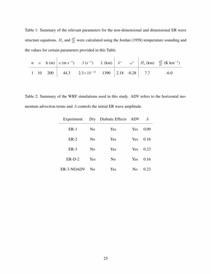
Table 1: Summary of the relevant parameters for the non-dimensional and dimensional ER wave

structure equations. Hs and dT̄dz

were calculated using the Jordan (1958) temperature sounding and

the values for certain parameters provided in this Table.

n a h (m) c (m s−1) β (s−1) L (km) k∗ ω∗ Hs (km) dT̄dz

(K km−1)

1 10 200 44.3 2.3×10−11 1390 2.18 -0.28 7.7 -6.0

Table 2: Summary of the WRF simulations used in this study. ADV refers to the horizontal mo-

mentum advection terms and A controls the initial ER wave amplitude.

Experiment Dry Diabatic Effects ADV A

ER-1 No Yes Yes 0.09

ER-2 No Yes Yes 0.16

ER-3 No Yes Yes 0.23

ER-D-2 Yes No Yes 0.16

ER-3-NOADV No Yes No 0.23

25

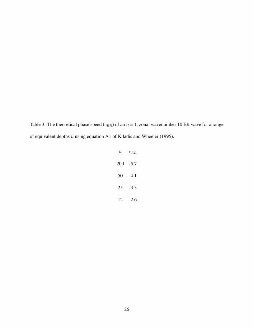
Table 3: The theoretical phase speed (cER) of an n = 1, zonal wavenumber 10 ER wave for a range

of equivalent depths h using equation A1 of Kiladis and Wheeler (1995).

h cER

200 -5.7

50 -4.1

25 -3.3

12 -2.6

26

List of Figures

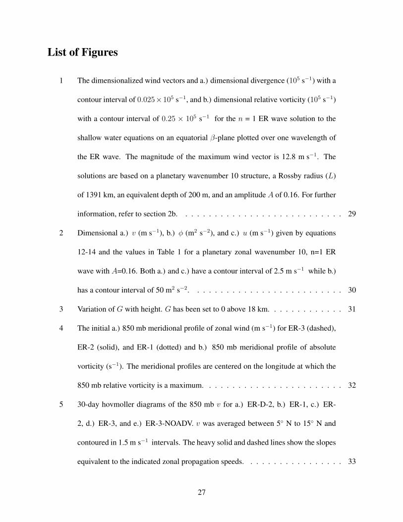
1 The dimensionalized wind vectors and a.) dimensional divergence (105 s−1) with a

contour interval of 0.025×105 s−1, and b.) dimensional relative vorticity (105 s−1)

with a contour interval of 0.25 × 105 s−1 for the n = 1 ER wave solution to the

shallow water equations on an equatorial β-plane plotted over one wavelength of

the ER wave. The magnitude of the maximum wind vector is 12.8 m s−1. The

solutions are based on a planetary wavenumber 10 structure, a Rossby radius (L)

of 1391 km, an equivalent depth of 200 m, and an amplitude A of 0.16. For further

information, refer to section 2b. . . . . . . . . . . . . . . . . . . . . . . . . . . . 29

2 Dimensional a.) v (m s−1), b.) φ (m2 s−2), and c.) u (m s−1) given by equations

12-14 and the values in Table 1 for a planetary zonal wavenumber 10, n=1 ER

wave with A=0.16. Both a.) and c.) have a contour interval of 2.5 m s−1 while b.)

has a contour interval of 50 m2 s−2. . . . . . . . . . . . . . . . . . . . . . . . . . 30

3 Variation of G with height. G has been set to 0 above 18 km. . . . . . . . . . . . . 31

4 The initial a.) 850 mb meridional profile of zonal wind (m s−1) for ER-3 (dashed),

ER-2 (solid), and ER-1 (dotted) and b.) 850 mb meridional profile of absolute

vorticity (s−1). The meridional profiles are centered on the longitude at which the

850 mb relative vorticity is a maximum. . . . . . . . . . . . . . . . . . . . . . . . 32

5 30-day hovmoller diagrams of the 850 mb v for a.) ER-D-2, b.) ER-1, c.) ER-

2, d.) ER-3, and e.) ER-3-NOADV. v was averaged between 5◦ N to 15◦ N and

contoured in 1.5 m s−1 intervals. The heavy solid and dashed lines show the slopes

equivalent to the indicated zonal propagation speeds. . . . . . . . . . . . . . . . . 33

27

6 The t = 30 d ER-D-2 500 mb vertical velocity (103 m s−1; shaded) with a.) the

850 mb wind vectors and 850 mb relative vorticity (105 s−1; contoured) and b.) the

200 mb wind vectors and 200 mb relative vorticity (105 s−1; contoured). . . . . . . 34

7 Vertical profile of the temporal evolution of the domain-averaged temperature per-

turbation from t = 0 for a.) ER-1 and b.) ER-2. Pressure is plotted on a logarithmic

scale. The contour interval is 1 K. . . . . . . . . . . . . . . . . . . . . . . . . . . 35

8 The t = 30 d ER-2 850 mb wind vectors and a.) the sea-level pressure (mb), b.) the

850 mb relative humidity, and c.) the 850 mb vertical velocity (m s−1). sea-level

pressure <1012.5, RH>0.80, and vertical velocities >0.025 m s−1 are shaded. . . . 36

9 Four quadrant summary of the ER-2 (ER-1 values in parentheses) t = 30 d 106×

850 mb relative vorticity, 106× 850 mb divergence, 200 - 850 mb zonal shear,

200 - 850 mb meridional shear, and 103× 850 mb vertical velocity averaged be-

tween 3◦ N and 12◦ N, and composited over all 10 wavelengths. The quadrant

boundaries in the zonal direction were determined by the 850 mb meridional wind

local maxima/minima and sign changes at a latitude of 7.5◦ N. . . . . . . . . . . . 37

10 The ER-3 sea-level pressure field (mb) over two arbitrary wavelengths at a.) t = 20 d,

b.) 22 d, c.) 24 d, and d.) 26 d. The continents are provided for reference only. . . . 38

11 The ER-3 850 mb wind vectors (a-c) and ER-3-NOADV 850 mb wind vectors (d-f)

at t = 11 d (a,d), t = 14 d (b,e), and t = 17 d (c,f). The jagged line in b.) denotes

the location of the inverted trough. The solid line in d.) indicates the zonal scale of

the cyclonic gyre of the ER wave and the zonal scale of the smaller-scale cyclonic

disturbance. . . . . . . . . . . . . . . . . . . . . . . . . . . . . . . . . . . . . . . 39

28

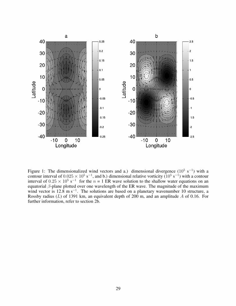
Figure 1: The dimensionalized wind vectors and a.) dimensional divergence (105 s−1) with acontour interval of 0.025× 105 s−1, and b.) dimensional relative vorticity (105 s−1) with a contourinterval of 0.25 × 105 s−1 for the n = 1 ER wave solution to the shallow water equations on anequatorial β-plane plotted over one wavelength of the ER wave. The magnitude of the maximumwind vector is 12.8 m s−1. The solutions are based on a planetary wavenumber 10 structure, aRossby radius (L) of 1391 km, an equivalent depth of 200 m, and an amplitude A of 0.16. Forfurther information, refer to section 2b.

29

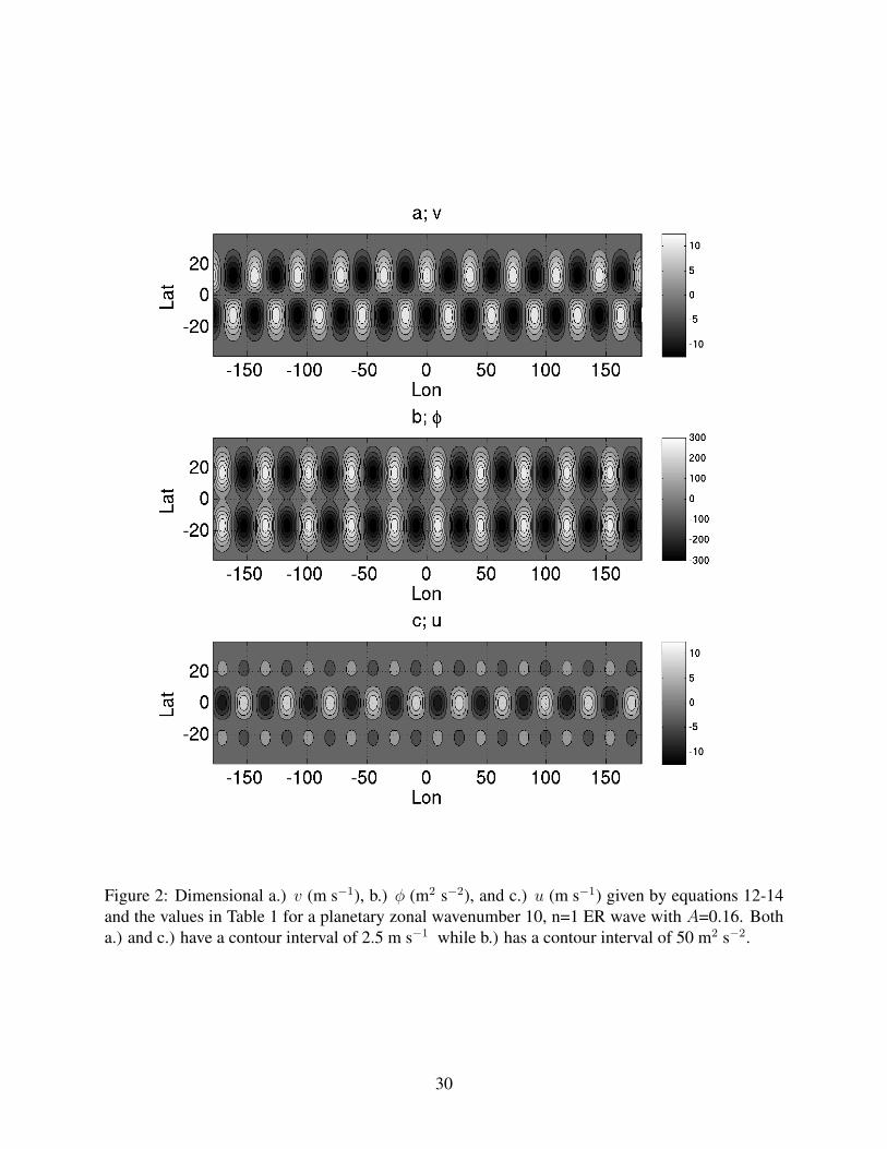
Figure 2: Dimensional a.) v (m s−1), b.) φ (m2 s−2), and c.) u (m s−1) given by equations 12-14and the values in Table 1 for a planetary zonal wavenumber 10, n=1 ER wave with A=0.16. Botha.) and c.) have a contour interval of 2.5 m s−1 while b.) has a contour interval of 50 m2 s−2.

30

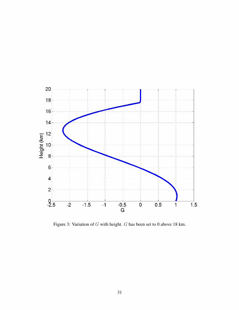
Figure 3: Variation of G with height. G has been set to 0 above 18 km.

31

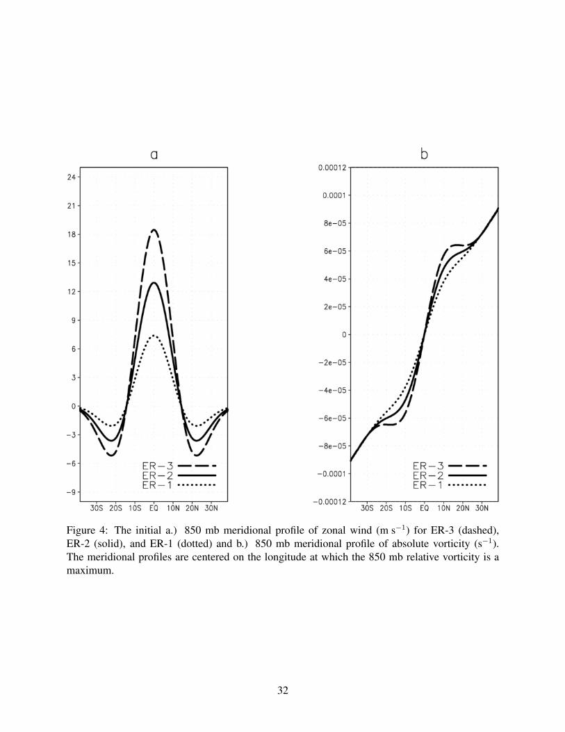
Figure 4: The initial a.) 850 mb meridional profile of zonal wind (m s−1) for ER-3 (dashed),ER-2 (solid), and ER-1 (dotted) and b.) 850 mb meridional profile of absolute vorticity (s−1).The meridional profiles are centered on the longitude at which the 850 mb relative vorticity is amaximum.

32

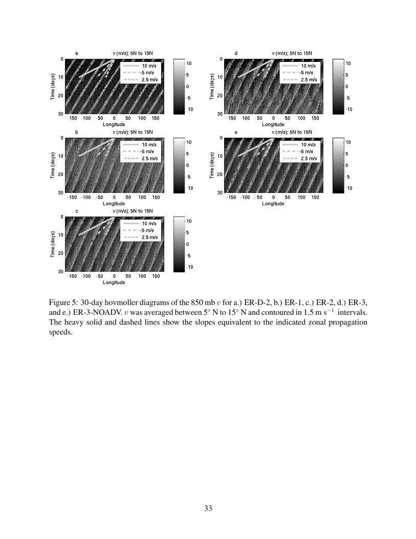
Figure 5: 30-day hovmoller diagrams of the 850 mb v for a.) ER-D-2, b.) ER-1, c.) ER-2, d.) ER-3,and e.) ER-3-NOADV. v was averaged between 5◦ N to 15◦ N and contoured in 1.5 m s−1 intervals.The heavy solid and dashed lines show the slopes equivalent to the indicated zonal propagationspeeds.

33

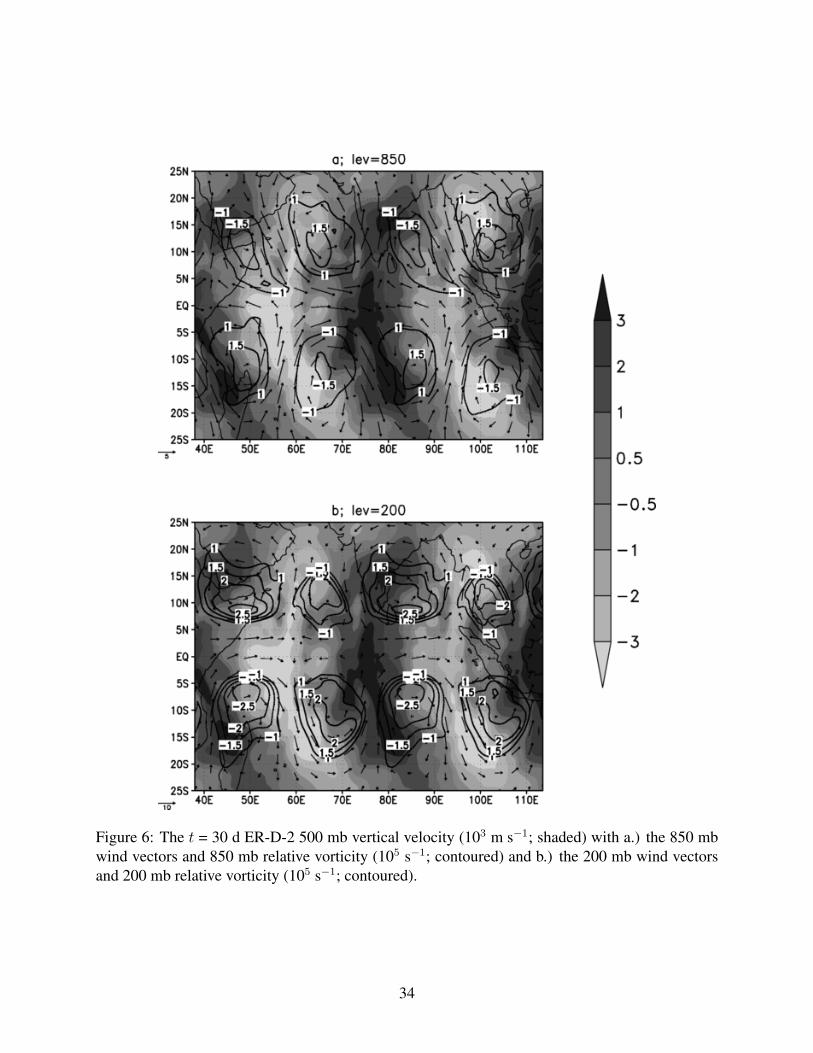
Figure 6: The t = 30 d ER-D-2 500 mb vertical velocity (103 m s−1; shaded) with a.) the 850 mbwind vectors and 850 mb relative vorticity (105 s−1; contoured) and b.) the 200 mb wind vectorsand 200 mb relative vorticity (105 s−1; contoured).

34

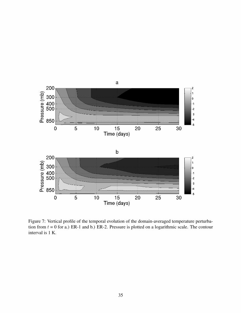
Figure 7: Vertical profile of the temporal evolution of the domain-averaged temperature perturba-tion from t = 0 for a.) ER-1 and b.) ER-2. Pressure is plotted on a logarithmic scale. The contourinterval is 1 K.

35

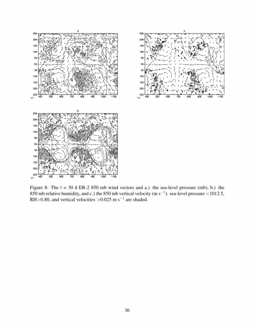
Figure 8: The t = 30 d ER-2 850 mb wind vectors and a.) the sea-level pressure (mb), b.) the850 mb relative humidity, and c.) the 850 mb vertical velocity (m s−1). sea-level pressure <1012.5,RH>0.80, and vertical velocities >0.025 m s−1 are shaded.

36

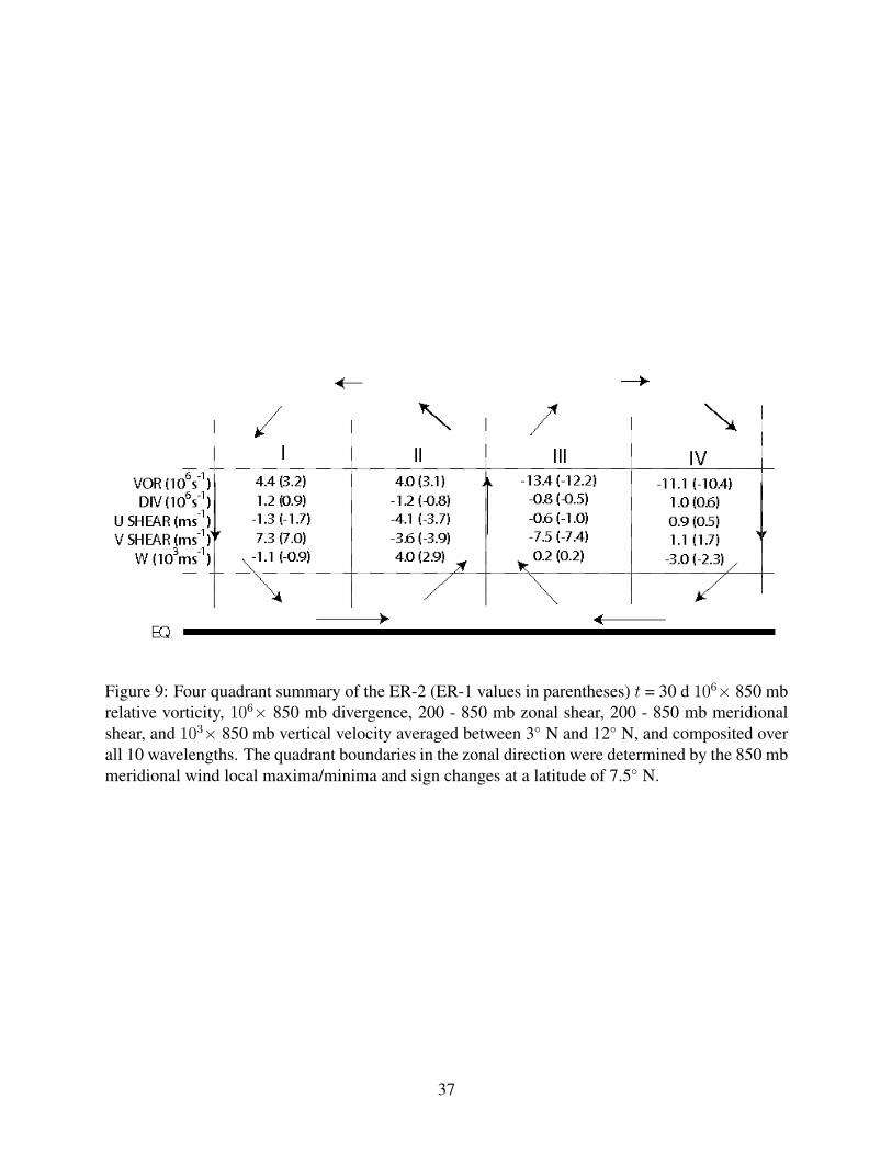
Figure 9: Four quadrant summary of the ER-2 (ER-1 values in parentheses) t = 30 d 106× 850 mbrelative vorticity, 106× 850 mb divergence, 200 - 850 mb zonal shear, 200 - 850 mb meridionalshear, and 103× 850 mb vertical velocity averaged between 3◦ N and 12◦ N, and composited overall 10 wavelengths. The quadrant boundaries in the zonal direction were determined by the 850 mbmeridional wind local maxima/minima and sign changes at a latitude of 7.5◦ N.

37

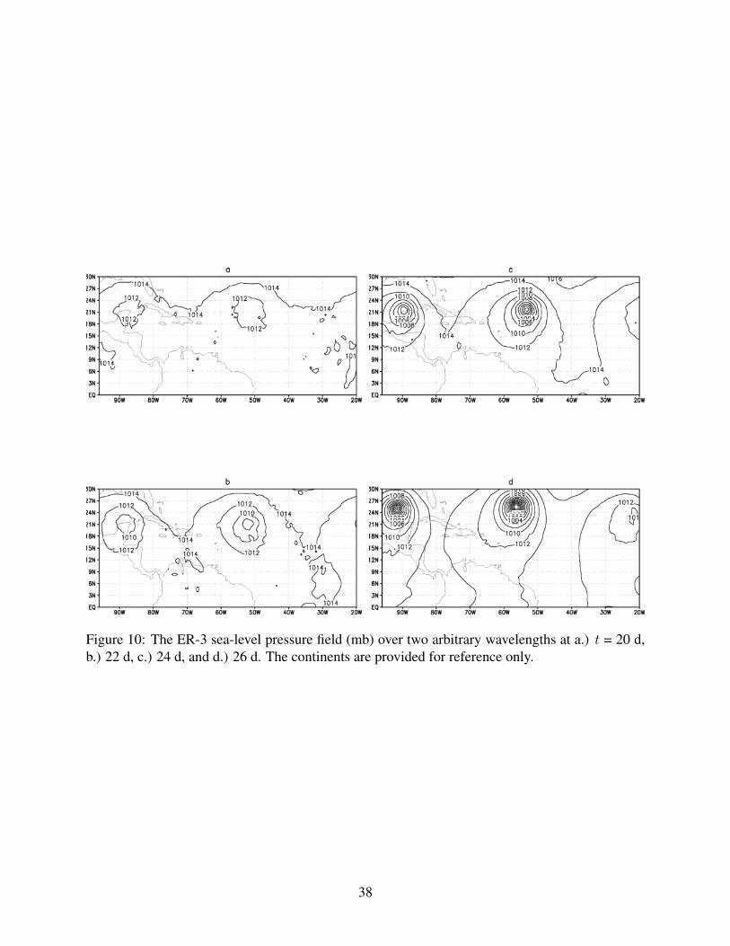
Figure 10: The ER-3 sea-level pressure field (mb) over two arbitrary wavelengths at a.) t = 20 d,b.) 22 d, c.) 24 d, and d.) 26 d. The continents are provided for reference only.

38

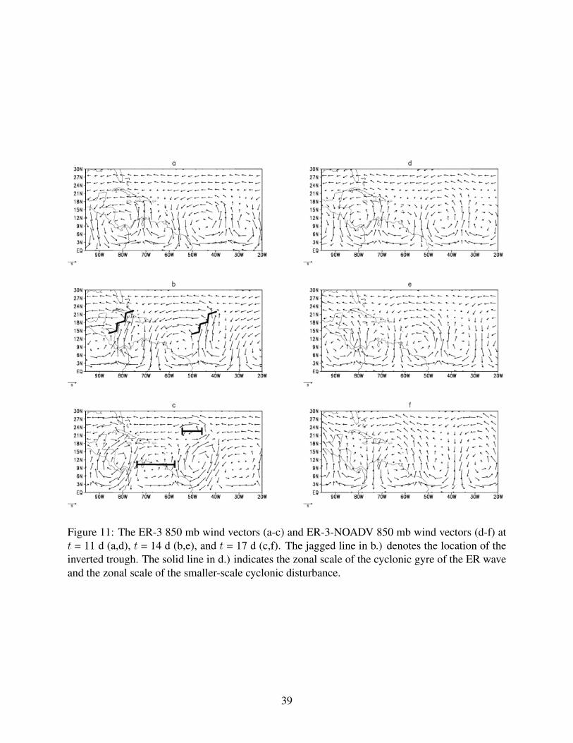
Figure 11: The ER-3 850 mb wind vectors (a-c) and ER-3-NOADV 850 mb wind vectors (d-f) att = 11 d (a,d), t = 14 d (b,e), and t = 17 d (c,f). The jagged line in b.) denotes the location of theinverted trough. The solid line in d.) indicates the zonal scale of the cyclonic gyre of the ER waveand the zonal scale of the smaller-scale cyclonic disturbance.

39