the role of fuzzy logic in gis modelling philippe puig13224/thesis_cdu_13224_puig_… · the role...
TRANSCRIPT

The role of fuzzy logic in GIS modelling
Philippe Puig
DEUG de Science
Licence de Géologie appliquée
Maitrise de Géologie appliquée
D.E.A. de Géologie appliquée
Graduate Diploma in Education (Secondary)
Graduate Diploma in Geographic Information
Faculty of Engineering, Health, Science and the
Environment
Charles Darwin University
PhD thesis
2011

Philippe Puig – PhD thesis
ii
Thesis declaration
I hereby declare that the work herein, now submitted as a thesis for the degree of
Doctor of Philosophy of the Charles Darwin University, is the result of my own
investigations, and all references to ideas and work of other researchers have been
specifically acknowledged. I hereby certify that the work embodied in this thesis has
not already been accepted in substance for any degree, and is not being currently
submitted in candidature for any other degree.
Philippe Puig
Date: 7 April, 2011

Philippe Puig – PhD thesis
iii
ACKNOWLEDGMENTS
This research was carried out in Darwin, in the Northern Territory of Australia,
between 2001 and 2010, while working full time on a variety of GIS projects in the
Top End of the Northern Territory. During that relatively long period of time both
my professional and my research environments changed.
Within that context, first and foremost, I am deeply indebted to my wife Patricia and
my two sons, Julien and Guillaume, who provided a stability and support in my
private life without which I would not have been able to complete this work.
Without the guidance and friendly encouragement of my two supervisors, Dr Diane
Pearson and Dr Stefan Maier, this thesis would not have been written. I thank them
for their unflinching support, their expert advice and their confidence in my
capabilities.
In addition to those I named before, many more persons and organisations
contributed to my research. Out of fear of unfairly forgetting some, I decided to
express my deepest gratitude to all relatives, friends, colleagues, professionals and
researchers who played a role in my endeavour.

Philippe Puig – PhD thesis
iv
GLOSSARY
AAGIS Anindilyakwa Aquaculture GIS
AHP Analytic Hierarchy Process
AI Artificial Intelligence
BOM Bureau Of Meteorology
CI Consistency Index
COG Centre Of Gravity
CR Consistency Ratio
DAC Darwin Aquaculture Centre
DEM Digital Elevation Model
DOF Degree Of Fulfillment
EDA Exploratory Data Analysis
FCM Fuzzy C-Means
FIS Fuzzy Inference System
FKC Fuzzy K-Clustering
GIS Geographic Information System
GAM Generalised Additive Model
GLM Generalised Linear Model
GK Gustafson Kessel (algorithm)
KBS Knowledge Based System
KE Knowledge Engineering
MAUP Modifiable Areal Unit Problem
MCDA Multi Criteria Decision Analysis
MF Membership Function
MOM Mean Of Maxima
NRM Natural Resource Management
NT Northern Territory
sciFLT Scilab Fuzzy Logic Toolbox
SMI Semantic Import Approach
TFN Trapezoidal Fuzzy Number
TRF Timor Reef Fishery
TS Takagi Sugeno

Philippe Puig – PhD thesis
v
UBC University of British Columbia
XLFIS Excel Fuzzy Inference System

Philippe Puig – PhD thesis
vi
Table of contents
1. Introduction
Scope of this thesis 2
1.1 Background 2
1.2 Geography and linguistic uncertainty 6
1.3 Statistical uncertainty and quantitative geography 8
1.4 Outline of this thesis 12
2. Some fundamental concepts of fuzzy logic
Overview 15
2.1 Models and modelling methods 15
2.2 Fuzzy sets and membership functions 18
2.3 Fuzziness, statistics and uncertainty 28
2.4 GIS, raster and direct application of membership functions 29
2.5 Acquisition of membership functions 34
2.6 Manual design of membership functions 43
2.7 Structure and functions of a fuzzy rule-based model 52
2.8 Implementation of a fuzzy rule-based model 62
Summary 67
3. GIS fuzzy multicriteria decision analysis
Overview 70
3.1 Background 72
3.2 Method and data 73
3.3 Results 83
3.4 Discussion 87
Summary 90
4. Data driven fuzzy rule-based modelling
Overview 93
4.1 Application of fuzzy rule-based modelling to classification 94
4.2 Multivariate predictive modelling on the basis of variables 106
of unknown influence on the outcome
4.3 What drives elephant seals’ foraging patterns? 122
Summary 130

Philippe Puig – PhD thesis
vii
5. Knowledge driven fuzzy rule-based modelling
Overview 133
5.1 Knowledge versus data driven fuzzy rule-based modelling 134
5.2 The need to capture human knowledge 138
5.3 Modelling fishing power from fishers’ knowledge 142
5.4 Implementation and applications of a functional fuzzy 155
rule-based expert system
Summary 164
6 Conclusion
Overview 168
6.1 Material presented in this thesis 168
6.2 What the case studies presented in this thesis tell us 170
6.3 Future directions of research in GIS applications of fuzzy 172
logic
6.4 What is the role of fuzzy logic in GIS modelling? 176
Summary 177
References 179

Philippe Puig – PhD thesis
viii
Appendices
Appendix 1 Excel Fuzzy Inference System XLFIS A-1
A1.1 Introduction to XLFIS A-1
A1.2 MODEL worksheet A-6
A1.3 IO and S_IO worksheets A-6
A1.4 V worksheets A-8
Appendix 2 Anindilyakwa Aquaculture GIS A-13
A2.1 Prawn farming suitability criteria A-13
A2.2 Some strategies to generate fuzzy maps A-16
A2.3 AAGIS source data A-18
A2.4 Calculation of AHP weightings A-20
Appendix 3 Data driven fuzzy-rule based modelling A-22
A3.1 Fisher’s iris dataset A-22
A3.2 Output membership values calculated by Fuzme for 5 clusters A-26
A3.3 Fuzzy rule-based modelling with Scilab A-30
A3.4 Elephant seals dataset A-33
Appendix 4 Knowledge driven modelling A-35
A4.1 Deriving membership functions from questionnaires A-35
A4.2 Introduction to sciFLT, a fuzzy logic toolbox for Scilab A-37
A4.3 Cheung’s comments on calculations of vulnerability to fishing A-47
pressure of Pristipomoides multidens
Philippe Puig – PhD thesis
ix
Tables
Table 2.1 ………………………………………………………… 22
Comparison of membership values of all integer values of X in Figure
2.1 and 2.2.
Table 2.2 ………………………………………………………… 50
Membership function coordinates derived from panel E in Figure 2.11.
Table 2.3 ………………………………………………………… 51
Fuzzy patch properties derived from panel E in Figure 2.11.
Table3.1 ………………………………………………………… 75
Source data sets of AAGIS.
Table 3.2 ………………………………………………………… 75
Criteria used to assess the suitability of prawn farming sites
Table 3.3 ………………………………………………………… 77
Relative importance of criteria assessed by pair wise comparisons.
Table 3.4 ………………………………………………………… 77
Values of relative importance used in suitability criteria pair wise
comparisons.
Table 3.5 ………………………………………………………… 79
Values of relative importance of criteria C1 to C5.
Table 3.6 ………………………………………………………… 79
Weightings of criteria C1 to C5.
Table 3.7 ………………………………………………………… 80
Evaluation of weightings’ consistency.
Table 3.8 ………………………………………………………… 80
Weightings of suitability criteria considered in AAGIS.
Table 3.9 ………………………………………………………… 81
Classes of suitability expressed in linguistic terms.
Table 3.10 ………………………………………………………… 82
Membership functions representing linguistic terms of suitability.
Table 4.1 ………………………………………………………… 94
Flower metrics used to classify iris flowers.

Philippe Puig – PhD thesis
x
Table 4.2 ………………………………………………………… 99
Values of flower metrics of the iris varieties considered.
Table 4.3 ………………………………………………………… 100
Input membership functions of fuzzy flower metrics.
Table 4.4 ………………………………………………………… 101
Output membership functions of Boolean iris varieties.
Table 4.5 ………………………………………………………… 104
Evaluation of the fuzzy classifier performance.
Table 4.6 ………………………………………………………… 111
Nakanishi’s dataset used in the simplified identification method.
Table 4.7 ………………………………………………………… 112
Effect of number of clusters on class size disparity.
Table 4.8 ………………………………………………………… 115
Vertex coordinates of output trapezoidal membership functions.
Table 4.9 ………………………………………………………… 118
Membership function coordinates of variables derived from a detailed
visual examination of plots in Appendix 3.
Table 5.1 ………………………………………………………… 147
Recalibrating estimates to compensate for informant’s bias.
Table 5.2 ………………………………………………………… 148
Rescaled informants’ estimates.
Table 5.3 ………………………………………………………… 149
Membership functions for medium values of fishing power.
Table 5.4 ………………………………………………………… 151
Membership functions of a fuzzy rule-based model of fishing power.
Table 5.5 ………………………………………………………… 152
List of rules of the fuzzy model of fishing power.
Table 5.6 ………………………………………………………… 160
Rules from Cheung’s expert system retained in the model of fish
vulnerability to fishing pressure in the TRF.
Table 5.7 ………………………………………………………… 161
Vulnerability to fishing pressure.
Table A1.1 ………………………………………………………… A – 6
Example of an IO worksheet of XLFIS.

Philippe Puig – PhD thesis
xi
Table A1.2 ………………………………………………………… A - 7
Example of S_IO worksheet of XLFIS.
Table A1.3 ……………………………………………………… A - 9
Functional blocks of the input data membership calculation sheet.
Table A2.1 ……………………………………………………… A - 20
Calculations of AHP weightings
Table A3.1 ………………………………………………………… A - 23
Fisher’s iris dataset (1 of 3).
Table A3.2 ………………………………………………………… A - 24
Fisher’s iris dataset (2 of 3).
Table A3.3 ………………………………………………………… A - 25
Fisher’s iris dataset (3 of 3).
Table A3.4 ………………………………………………………… A - 33
Variables of the fuzzy model for elephant seals foraging patterns (1 of 2)
Table A3.5 ………………………………………………………… A - 34
Variables of the fuzzy model for elephant seals foraging patterns (2 of 2).
Table A4.1 ………………………………………………………… A - 35
Example of binary transcription of informant’s records to a scratchpad.
Table A4.2 ………………………………………………………… A - 36
Tally of informants’ scores.
Table A4.3 ………………………………………………………… A - 36
Display of membership function parameters that summarise
informants’ views.

Philippe Puig – PhD thesis
xii
Figures
Figure 2.1 ………………………………………………………… 19
Overlapping fuzzy membership functions showing that classes in
fuzzy logic are not mutually exclusive.
Figure 2.2 ………………………………………………………… 21
Membership functions in binary logic are non overlapping and
rectangular.
Figure 2.3 ………………………………………………………… 23
Bell shaped membership function proposed by Burrough.
Figure 2.4 ………………………………………………………… 25
Two commonly used piecewise linear membership functions:
trapezoidal (MF1) and triangular (MF2).
Figure 2.5 ………………………………………………………… 27
A membership function and its definition by α-cuts.
Figure 2.6 ………………………………………………………… 32
Trapezoidal membership function defining three possible values of
suitability.
Figure 2.7 ………………………………………………………… 33
A method to translate linguistic suitability into rasters.
Figure 2.8 ………………………………………………………… 39
Graphical representation of the concept of fuzzy patch.
Figure 2.9 ………………………………………………………… 41
Membership functions reliability and overlap.
Figure 2.10 ………………………………………………………… 46
Fuzzy patches graphically associate input and output data.
Figure 2.11 ………………………………………………………… 47
The six stages of the identification process.
Figure 2.12 ………………………………………………………… 54
Four fundamental processes of a fuzzy rule-based model.
Figure 2.13 ………………………………………………………… 62
Comparison of MOM and COG defuzzification methods.
Philippe Puig – PhD thesis
xiii
Figure 2.14 ………………………………………………………… 63
The model definition GUI of the Scilab fuzzy logic toolbox sciFLT.
Figure 2.15 ………………………………………………………… 64
Membership function definition in sciFLT.
Figure 2.16 ………………………………………………………… 65
Rule definition in sciFLT.
Figure 2.17 ………………………………………………………… 65
Summary of universal approximator model characteristic features.
Figure 2.18 ………………………………………………………… 66
Model predictions plotted against experimental values.
Figure 3.1 ………………………………………………………… 70
Location of the Anindilyakwa Aquaculture GIS (AAGIS) project.
Figure 3.2 ………………………………………………………… 84
Maps showing the suitability of Groote Eylandt to aquaculture.
Figure 3.3 ………………………………………………………… 85
Details of suitability maps.
Figure 3.4 ………………………………………………………… 86
Groote Eylandt regions of highest suitability to prawn aquaculture
Figure 3.5 ………………………………………………………… 87
Aerial view of one area identified as suitable for prawn farming.
Figure 4.1 ………………………………………………………… 95
Plots of iris varieties versus flower metrics.
Figure 4.2 ………………………………………………………… 97
Membership functions petal length and petal width for 3 iris varieties.
Figure 4.3 ………………………………………………………… 98
Membership functions of sepal length and sepal width.
Figure 4.4 ………………………………………………………… 102
The Matlab visualisation of a fuzzy model architecture.
Figure 4.5 ………………………………………………………… 103
The Matlab visualisation of rules firing.
Figure 4.6 ………………………………………………………… 105
Correlation between outputs of the weighted and non weighted models.
Figure 4.7 ………………………………………………………… 112
Assessment of the optimum number of classes in the model.

Philippe Puig – PhD thesis
xiv
Figure 4.8 ………………………………………………………… 114
Extracting membership function by fuzzy clustering.
Figure 4.9 ………………………………………………………… 115
Plots of membership values showing a clear contrast between variables.
Figure 4.10 ………………………………………………………… 118
Plots of experimental records versus membership values of variables.
Figure 4.11 ………………………………………………………… 119
Evaluation of the predictive capability of Nakanishi’s model.
Figure 4.12 ………………………………………………………… 120
Evaluation of the lower predictive capability of the simplified model.
Figure 4.13 ………………………………………………………… 126
Comparison of PCTIME and TIME membership functions.
Figure 4.14 ………………………………………………………… 127
Effect of the absence of correlation between input and output variables.
Figure 5.1 ………………………………………………………… 140
Location of the Timor Reef Fishery.
Figure 5.2 ………………………………………………………… 141
Map of TRF commercial productivity.
Figure 5.3 ………………………………………………………… 144
One of 5 similar sheets making up the fishing power questionnaire.
Figure 5.4 ………………………………………………………… 146
Experts estimate the fishing power of key features of fishing vessels
of the TRF.
Figure 5.5 ………………………………………………………… 150
Membership functions of fishing power of fishing units.
Figure 5.6 ………………………………………………………… 151
Input membership functions of fishing power displayed by sciFLT.
Figure 5.7 ………………………………………………………… 153
Predictive capability of the initial model of fishing power.
Figure 5.8 ………………………………………………………… 158
First 4 input variables of Cheung’s expert system.
Figure 5.9 ………………………………………………………… 159
Last 4 input variables of Cheung’s expert system.

Philippe Puig – PhD thesis
xv
Figure 5.10 ………………………………………………………… 160
Output variable of Cheung’s expert system.
Figure 5.11 ………………………………………………………… 162
3D plot of intrinsic vulnerability of the Goldband snapper.
Figure A1.1 ………………………………………………………… A - 2
2004 presentation on fuzzy rule-based modelling given to Fisheries.
Figure A1.2 ………………………………………………………… A - 3
B.
Figure A1.3 ………………………………………………………… A - 5
Summary worksheet of XLFIS.
Figure A1.4 ………………………………………………………… A - 12
Principles of calculation of membership of input values in XLFIS.
Figure A2.1 ………………………………………………………… A - 21
Spreadsheet for the calculation of AHP weightings.
Figure A3.1 ………………………………………………………… A - 29
Trapezoidal membership functions derived from projecting Y class
memberships on independent variable X1.
Figure A3.2 ………………………………………………………… A - 29
Trapezoidal membership functions derived from projecting Y class
memberships on independent variable X3.
Figure A3.3 ………………………………………………………… A - 30
Properties of the fuzzy rule-based models supported by sciFLT.
Figure A3.4 ………………………………………………………… A - 31
Graphs of membership functions generated by Scilab FLT.
Figure A3.5 ………………………………………………………… A - 32
Rules pane in sciFLT..
Figure A4.1 ………………………………………………………… A - 37
Membership function summarising informants’ views.

Philippe Puig – PhD thesis
xvi
Equations
Equation group 2.1 ………………………………………………… 19
Equation group 2.2 ………………………………………………… 20
Equation 2.1 ………………………………………………… 23
Equation group 2.3 ………………………………………………… 24
Equation group 2.4 ………………………………………………… 25
Equation group 2.5 ………………………………………………… 25
Equation group 2.6 ………………………………………………… 26
Equation 2.2 ………………………………………………… 45
Equation 2.3 ………………………………………………… 57
Equation 2.4 ………………………………………………… 57
Equation 2.5 ………………………………………………… 57
Equation 2.6 ………………………………………………… 58
Equation group 2.7 ………………………………………………… 59
Equation 3.1 ………………………………………………… 78
Equation 5.1 ………………………………………………… 139
Equation A1.1 ………………………………………………… A - 11
Equation A1.2 ………………………………………………… A - 11
Equation group A1.1 ………………………………………………… A - 12

Philippe Puig – PhD thesis
xvii
Abstract
This thesis investigates the application of fuzzy logic to geospatial problems. Fuzzy
logic provides a means for dealing with vague information and sparse datasets
inherent to many real world applications. A fuzzy site suitability analysis for prawn
farming on remote Groote Eylandt demonstrates how fuzzy logic concepts can be
incorporated into maps to facilitate site selection.
Another application presented relies on a published chemical plant operation dataset
to illustrate how data driven modelling enables objective predictions on the basis of
available information. In a third application, records of environmental variables
associated with the foraging patterns of elephant seals are reinterpreted. The fuzzy
rule-based data driven analysis of this small dataset of high dimensionality leads to
an unambiguous conclusion more efficiently than other methods described in the
literature.
Knowledge driven fuzzy rule-based modelling is illustrated by case studies aimed at
improving the sustainability of the Timor Reef fishery. Firstly, the knowledge of
experienced fishers is recorded to evaluate the fishing power of the Timor Reef
fishery fleet to assess the need for recalibrating an existing map of productivity. Near
constant fishing power across that fleet suggests that recalibration is not necessary.
Secondly, a published fuzzy rule-based expert system is implemented. It can estimate
fish susceptibility to fishing pressure from biological parameters only. The
susceptibility to fishing pressure of target species of the Timor Reef fishery,
estimated with this fuzzy expert system, differs from that estimated from globally
averaged parameters. These discrepancies highlight the importance of local models
for the development of sustainable fisheries.
Case studies in this thesis highlight the potential of fuzzy rule-based modelling in
complementing statistical methods applied to spatial problems particularly when the
uncertainty of the data is undefined. That potential is noteworthy in marine natural
resource management.

CHAPTER 1
INTRODUCTION

Philippe Puig – PhD thesis
- 2 -
Scope of this thesis
This thesis demonstrates that fuzzy logic simplifies GIS modelling by providing a
generic approach to predictions on the basis of a wide range of data.
GIS models often rely on non spatial predictive capabilities including curve fitting,
classification and multivariate analysis that are provided by a variety of statistical
modelling techniques. This dissertation argues that fuzzy rule-based modelling offers,
in one single coherent framework, a valid alternative to the variety of statistical
modelling techniques currently relied on to perform these tasks. Fuzzy rule-based
modelling can be either data, or knowledge driven, and therefore provides GIS
modelling with additional flexibility, much needed in Natural Resource Management.
The objectives of this dissertation are to first provide an underlying rationale for the
adoption of fuzzy logic instead of Boolean logic to describe uncertainty within the
geographical context of GIS. The second objective is to introduce the reader to the
fundamentals of fuzzy logic required to understand the case studies which support
the central claim of this thesis. The third objective is to explore a non fuzzy rule-
based modelling method, more intimately integrated in the GIS methodology, yet
lacking the multi purpose capabilities of fuzzy rule-based modelling. The fourth
objective is to explore case studies which support the hypothesis that fuzzy rule-
based modeling offers a valid alternative to statistical modeling techniques. The last
objective is to emphasise the relevance of fuzzy rule-based modelling in GIS models
for the management of natural resources particularly aquaculture and fisheries in
Australia, and more specifically in the Northern Territory, and other similar parts of
the world.
1.1 Background
Geographic Information System (GIS) originated in Canada from the work of
Tomlinson (Coppock and Rhind, 1991) in the 1960s. GIS was Tomlison‟s response
to an urgent need for substantial improvements in Natural Resource Management
(NRM). Typical GIS outputs include maps and modern cartographic elements such

Philippe Puig – PhD thesis
- 3 -
as digital elevation models (DEM), as well as other derived datasets, with or without
pictorial components. All are approximations of an infinitely complex natural world:
they are models. This thesis is concerned with the growing complexity and diversity
of methods adopted to develop these models. The sorites paradox (Fisher, 2000),
later discussed in this chapter, expresses our inability to translate numerically the
clear linguistic difference we make between a heap of sand and a dune. This
contradiction highlights an underlying cause for the pervasive failure of GIS to
adequately represent some fundamental geographical entities. The solution proposed
here, suggested by this paradox, is a radical change in the modelling framework that
prevails in GIS modeling. What fuzzy logic offers is a completely different definition
of uncertainty leading to a single, simplified modelling strategy capable of
complementing purely spatial components of GIS models as required. Non statistical
by design, the method advocated does not suffer from limitations of more main
stream strategies.
1.1.1 Trends in GIS modelling
Geography became more quantitative in the 1990s (Earickson and Harlin, 1994). As
the role of statistics grew, the approach of geography, with the advent of GIS,
became increasingly quantitative. Currently, predictive GIS modelling is generally
statistical in nature. Typified by the sophisticated Geographically Weighted
Regression (Fotheringham et al., 2002) it relies more and more on complex statistics.
Generalised Linear Models (Guisan et al., 2002; Bradshaw et al., 2004), as well as
alternative statistics such as Bayesian modelling; (Guisan and Zimmerman, 2000)
add to the plethora of statistical methods from which GIS modellers can choose.
GIS users in soil sciences (Burrough et al., 1992), as well as in geosciences
(Bonham-Carter, 1994), discovered the potential offered by fuzzy logic some time
ago. While soil scientists immediately saw in fuzzy logic a way to better describe
boundaries between soil types, geologists mainly saw applications for pattern
recognition and expert systems (Bonham-Carter, 1994). Soil classification relies on
strict definitions of materials resulting from gradual processes under highly variable
natural conditions. Irrespective of efforts from soil scientists, boundaries between
soil types cannot be made crisp. In the 1990s Burrough was joined by other soil

Philippe Puig – PhD thesis
- 4 -
scientists (Lagacherie et al., 1996). They came to the conclusion that the “new”
mathematical model proposed by Zadeh (1965), more than a quarter of a century
earlier, was better suited to pedology than the traditional mathematical framework
built on Boolean logic.
This dissertation proposes to revisit the concepts actively promoted by Burrough
nearly 20 years ago and focus on a direction which, at the time, had not been
sufficiently researched to reveal its full potential.
1.1.2 Fuzzy logic in GIS modelling
As GIS started to become more widely available (Leung, 1999), researchers became
increasingly concerned by its over-simplified description of the inherent uncertainty
of geographic data (Goodchild, 2000). They explored ways of designing more
conceptually realistic GIS models. Their solutions remained generally impractical
(Jeansoulin and Wurbel, 2003; Liu, 2003) and GIS, as we presently know it, still
relies on Boolean concepts. This thesis consequently explores practical ways of
merging the rather blunt, yet widely adopted, existing Boolean GIS framework with
an improved approach to reality through the adoption of fuzzy reasoning.
Before the start of the new millennium, few papers on spatial analysis (Wegener and
Fotheringham, 2000) refer to fuzzy logic. Only one paper by Wilson and Lorang
(2000) focuses on fuzzy logic to reveal its great potential to improve GIS erosion
modelling. The same year, a special issue of Fuzzy Sets and Systems presents 12
papers by some prominent GIS researchers. Goodchild (2000) is mindful of the
negative impact of additional levels of complexity on GIS which owes much of its
attraction to its simplicity. In 2000, research in applications of fuzzy logic to GIS
modelling does not appear to reach GIS modelling circles where it receives less
coverage than it deserves. Yet fuzzy logic researchers see in GIS a worthwhile
domain of application. Dubois, in his preface to “Fuzzy rule – based modelling with
applications to geophysical, biological and engineering systems” by Bardossy and
Duckstein (1995) gives three reasons why the fuzzy-rule based models are worth
considering. Firstly they apply to a large number of situations that cannot be
described by linear functions. Secondly they remain comparatively simple. Thirdly,

Philippe Puig – PhD thesis
- 5 -
they can be interpreted verbally. These three arguments are of considerable relevance
to GIS modelling where many “real life” environmental problems are hard to
describe by mathematical formulations simple enough to be implemented in a GIS
environment. The compatibility of fuzzy logic with human language is very
advantageous as modelling can become more accessible to non mathematicians and
more transparent to the public.
The quest for computational tools, that are conceptually more transparent to the
wider community, has lead to the development of „soft computing‟. This term was
coined by Zadeh in the early 1990's (Yen, 1999) to describe a family of new
computational tools, all aimed at improving existing computational techniques based
on fuzzy-logic. Among the best known are neural networks and genetic algorithms.
They have been associated with fuzzy logic, and particularly fuzzy rule-based
modelling, to better match predictions and observations. These tuning algorithms
often generate weightings that optimise model predictions. Although „soft
computing‟ techniques may play an important role in specific engineering
applications, such as control systems, they have two major drawbacks. They
substantially increase the complexity of the model and remove all transparency in
fuzzy rule-based modelling. Consequently „soft computing‟ is deliberately ignored in
this thesis.
Fuzzy logic has been unnecessarily associated, through „soft computing‟, with very
different computational frameworks such as neural networks. The resulting
confusion contributes to the difficulty of assessing the current standing of fuzzy logic
in GIS modeling. As demonstrated by the publication of a special issue of Fuzzy Set
(Cobb et al., 2000) on uncertainty in GIS and spatial data, a number of leading GIS
researchers are aware of the advantages offered by fuzzy logic. Yet, the role of fuzzy
logic in GIS modelling remains insignificant. This thesis offers a solution to this
apparent contradiction. Instead of focusing on the development of geographically
specific implementations of fuzzy logic, this thesis explores how GIS modelling can
benefit from simple and practical fuzzy logic techniques commonly used in
engineering.

Philippe Puig – PhD thesis
- 6 -
1.2 Geography and linguistic uncertainty
Paradoxes often reflect flaws in reasoning. Addressing inconsistencies in the logic
underpinning cognitive processes, and derived computations, can only lead to
improvements in the outcome. The „heap of sand‟ paradox (Fisher, 2000) below is
the first of two paradoxes which support the quest for an alternative GIS modelling
paradigm that drives this thesis.
1.2.1 A ‘heap of sand’ to test fuzziness
When does a clump of trees become a forest? How can we tell the boundary between
land and sea? We can all offer answers to these questions. However, they are likely
to be different. They reflect a particular type of vagueness captured by Greek
philosophers in the „heap of sand‟ paradox (Fisher, 2000). The “heap of sand”
(sorites in ancient Greek) paradox is defined in one question: What is a heap of sand?
In other words what is the critical number of grains of sand that makes a collection of
grains a heap. A geographical adaptation of this paradox could be: what is a forest?
One cannot define a heap of sand by adding individual grains until we obtain a heap
and nor can one define a forest by adding individual trees. This vagueness is not of
numerical nature but reflects instead our perception of the world. Fisher (2000)
concludes that this vagueness is better addressed by fuzzy logic, “Fuzzy set theory
provides a framework in which vagueness can not only be developed and
implemented, but can be analysed and sustained as a basis for exploration and
explanation” (Fisher, 2000: p.15).
Fisher (2000) proposes the „sorites paradox‟ as a simple test to assess the nature of
the underlying vagueness of geographical entities. If the geographical object
considered is affected by the sorites paradox, it cannot be defined by Boolean logic.
Statistics are consequently incapable of quantifying its underlying uncertainty.
However it is believed that fuzzy logic can.

Philippe Puig – PhD thesis
- 7 -
1.2.2 A paradigm shift
“Fuzzy sets and fuzzy logic” (Klir and Bo Yuan, 1995) contains a comprehensive
bibliography of 1731 titles. History and basic notions of fuzzy sets (Dubois et al.,
2000) are presented in the first of seven volumes making up the Handbooks of Fuzzy
Sets. This encyclopedia of fuzzy logic compiled by experts recognised world wide
for their contributions to fuzzy logic is a reference that reflects the interest generated
by fuzzy logic as a result of remarkable technological achievements at the end of the
twentieth century. Clearly, fuzzy logic is well documented and information on the
subject is readily available. Dubois and Prade (1994) deplore misinformed attacks
from proponents of statistics and Bayesian methods. To address the issue of
misinformation they embarked on detailed comparisons between fuzzy logic and
probability/statistics (Dubois and Prade, 1986, 1993). Hisdal (1988) offers an olive
branch to all parties by relying on probabilities to demonstrate fuzzy logic. As
respective merits of fuzzy logic and statistics have been so extensively debated
elsewhere they are not discussed in this thesis. The title of the first chapter of the
reference text “Fuzzy sets and fuzzy logic” reads “From classical (crisp) sets to fuzzy
sets: a grand paradigm shift” (Klir and Bo Yuan, 1995: p.1). Parallels between
Zadeh‟s „fuzzy logic‟ and theories such as Darwin‟s „evolution of species‟ or
Einstein‟s „relativity‟ are unmistakable. Both represent grand challenges to well
established, reputable domains of human knowledge. They are paradigm shifts. As
such they are initially rejected, criticised, scrutinised and eventually recognised.
1.2.3 Relevance of fuzzy logic to geography
The seminal paper “Fuzzy sets” (Zadeh, 1965) by a professor of electrical
engineering at Berkeley University stresses that “…, the notion of a fuzzy set is
completely non statistical in nature” (Zadeh, 1965: p. 340). Consequently fuzzy logic
should not suffer from any limitation of statistical modelling. Nearly 30 years later,
the influence of Zadeh‟s model of uncertainty is reflected in Bouchon Meunier's
introduction to “La logique floue” (1993: p. 3): “La logique floue suscite
actuellement un intérêt général de la part des chercheurs, des ingénieurs et des
industriels, mais plus généralement de la part de tous ceux qui éprouvent le besoin de
formaliser des méthodes empiriques, …”. Translated this means “Fuzzy logic

Philippe Puig – PhD thesis
- 8 -
generates much interest among researchers, engineers and industrialists but more
generally among all those who need to formalise empirical methods,…”.
Researchers in geography (Robinson et al., 1986; Leung, 1987; Robinson, 1988)
started to look at the potential of fuzzy logic in GIS at a time which predates the
rapidly growing research in fuzzy rule-based modeling which characterizes the 1990s.
Robinson et al. (1986) explores the role of expert systems in four GIS domains: map
design, feature extraction, database management and decision support systems.
Robinson (1988) later focuses on the applications of fuzzy logic geographic
databases. He only briefly mentions fuzzy logic. Leung (1987) focuses on the
application of fuzzy logic to the definition of boundaries but later (Leung, 1999)
considers spatial analysis as well. Burrough (1989) extensively explores this topic as
well as the role of fuzzy logic in classification (Burrough et al., 1992) in GIS.
Applications of fuzzy logic to mining exploration in GIS (Bonham-Carter, 1994)
appear. Research on applications of fuzzy logic to GIS has clearly been very active
(Mackay and Robinson, 2000; Dragicevic and Marceau, 2000; MacMillan et al.,
2000; Cobb et al., 2000; Guesguen and Albrecht, 2000; Robinson, 2000; Wang,
2000). However, only few practical applications emerged. A notable exception is the
fuzzy functionality available in the decision support system of the commercial GIS
software IDRISI (Eastman, 2009: p. 159). The effort committed to this domain of
research was not reflected in the significance of derived practical applications.
1.3 Statistical uncertainty and quantitative geography
First, the „sorites‟ paradox (Fisher, 2000) suggests that current GIS modeling
incorrectly represents some geographical concepts. The second paradox, outlined
below, indicates that our traditional statistical approach to uncertainty may have
flaws, addressed to some extent by geostatistics. The growing disinterest in
quantitative geography (Fotheringham et al., 2000) may reflect the inadequacy of the
current reliance on statistics to describe geographic uncertainty.
Karl Popper (2008), in his “Logic of Scientific discovery”, stumbles on a
fundamental paradox in the theory of chance, central to probability, the very
Philippe Puig – PhD thesis
- 9 -
foundation of statistics. “The most important application of the theory of probability
is to what we may call „chance-like‟ or „random‟ events, or occurrences. These seem
to be characterized by a peculiar kind of incalculability which makes one disposed to
believe – after many unsuccessful attempts – that all known rational methods of
prediction must fail in their case. We have, as it were, the feeling that not a scientist
but only a prophet could predict them. And yet, it is just this incalculability that
makes us conclude that the calculus of probability can be applied to these events.”
(Popper, 2008: p.138). The apparent paradoxical nature of probability calculations
suggests that we may need to reconcile the unpredictability of chance events with
predictions of their occurrence. Probabilistic reasoning developed from large
numbers of observations which generally reveal a convergence of outcomes of
random events such as getting a five when throwing a dice or drawing a queen of
spade from a pack of cards. The „fundamental problem of the theory of chance‟
(Popper, 2008: p.142) stems from the antithetic axioms of convergence, or limit, and
randomness central to the theory of probability. Convergence is hardly compatible
with randomness, as true randomness precludes the definition of a limit towards
which a series of numbers may tend. The somewhat limited randomness of chance
observations, from which probability taught in scientific courses emerged, betrays its
initial association with gaming. By contrast, many complex natural systems may
display a substantially more random behaviour resulting in a questionable
convergence of measurements recorded to describe the process investigated.
Bertrand Russell, one of the most influential thinkers of the twentieth century was
both a mathematician and a philosopher. His views cast some light on Popper‟s
paradox. Russel calls frequency theory the probability theory associated with
statistical inference (Russel, 2009b: p.630) derived from gaming. Russel (2009b)
does not consider that the frequency theory is characterised by the certainty expected
from mathematics. He argues that the frequency theory is closer to science than to
mathematics (Russel, 2009a: p.293). Russel (2009a), besides the frequency theory,
considers two notable alternative theories of probability. They are the theory of
mathematical probability and Keynes‟s theory of probability. Keynes, better known
for his work in economy, exposes in „Treatise of Probability‟ (1921) his deductive
logical-relationist theory of probability. The logical-relationist theory of probability
does not abide by the true and false dichotomy. His theory of probability includes the

Philippe Puig – PhD thesis
- 10 -
concept of degree of rational belief assigned to a proposition, a concept already
advocated by Leibniz (Keynes, 1921: p.2) at end of the eighteenth century. Keynes‟s
theory of probability, like the theory of mathematical probability, hinges upon a
logical relation between two sets of propositions (Keynes, 1921: p.8): a premiss and
a conclusion. Knowledge too plays an important role in this logical-relationist theory
(Keynes, 1921: p.18). Popper, Russel and Keynes grappled with unsatisfactory
aspects of the treatment of uncertain events in the frequency theory of probability.
Kolmogorov (1956), aware of inconsistencies in frequency theory, has made
fundamental contributions to the current theory of probability. Regardless of its
imperfections, no alternative to the theory has lead to numerical methods capable to
compete with statistical modelling for the prediction of uncertain outcomes in
domains. This statistical model, called statistical inference, consists in fitting the data
representative of a population to a model from which parameters are derived, to infer
uncertain properties of this population. Bayesian inference (Bayes, 1763), an
alternative to statistical inference, relies on a more subjective approach as it proposes
a prior distribution which, on the basis of new data, provides the basis for the
inference of a posterior distribution. Both inferential and Bayesian statistics strive to
predict uncertain events. The role of inferential statistics in linking cause and effect,
through statistical methods such as the analysis of variance (Fisher, 1925), has
substantially contributed to the advancement of science during the past century. Yet,
scientific knowledge is not only hampered by uncertainty, initially exemplified by
random outcomes in gaming, but by imprecision as well. The frequency theory,
however, only applies to uncertainty.
Lofty Zadeh (1965: p. 339) describes the concept of fuzzy sets as “…a natural way
of dealing with problems in which the source of imprecision is the absence of sharply
defined criteria of class membership rather than the presence of random variables”.
Zadeh (1978) derives, from the concept of fuzzy sets, a theory of possibility which
parallels the theory of probability (Dubois et al., 2004) and extends it by creating a
suitable framework for the treatment of imprecision. In one sentence, “… the
imprecision that is intrinsic in natural languages, is in the main, possibilistic rather
than probabilistic in nature” (Zadeh, 1978: p. 3), Zadeh hints at the major role that
fuzzy sets can play in interfacing between human languages and scientific
applications. The possibility theory complements the frequency theory. The former is

Philippe Puig – PhD thesis
- 11 -
best equipped to tackle uncertainty while the latter applies to both uncertainty and
imprecision. Fuzzy logic, based on fuzzy sets, did not prompt the philosophical
concerns expressed by Popper (2008) and Russel (2009). Like Keynes‟s theory of
probability, fuzzy logic is not dichotomous but can easily accommodate binary logic.
The formalism of fuzzy sets based reasoning relies on logical relations between an
antecedent and a conclusion, a framework reminiscent of the logical-relationist
probability (Keynes, 1921). The degree of fulfillment of a fuzzy rule and the degree
of belief of Keynes‟s theory (Keynes, 1921) bear some resemblance. Fuzzy sets, as
this thesis will demonstrate, offers a unified framework to process uncertainty and
imprecision (Bouchon-Meunier, 1999: p. 5). One can therefore imagine that the
domains of application of fuzzy logic overlap those of statistics as will be
demonstrated in this thesis. Bouchon-Meunier‟s (1999) views suggest that fuzzy
logic may complement statistics (Dubois and Prade, 1986) particularly when
vagueness of information is more closely related to imprecision than to uncertainty
or when advantages offered by a unified framework take precedence on the
sophistication of statistical methods. In addition fuzzy logic may be useful in
situations where the axiom of randomness, central to the frequency theory of
probability, cannot always be verified.
Krige, a South African mining engineer (Upton and Cook, 2008), came to the
conclusion that spatial processes cannot be ignored in the statistical description of
mineral resources. The independence of events, directly related to the randomness
that bothered Popper (Popper, 2008), rarely applies to geography. It turns out that
there is much to gain in studying that non randomness caused in that instance by the
spatial correlation of observations. In 1962 Matheron formalised Krige‟s work in his
“Treatise of applied geostatistics” (Upton and Cook, 2008) where he describes the
spatial interpolation called kriging. Although a clear departure from traditional
statistics in the sense that they clearly acknowledge the peculiarity of spatial data,
geostatistics still require data to be normally distributed, a frequent statistical
prerequisite to the applications of a number of modelling techniques. The need for
geostatistics suggests that, when it comes to spatial applications, statistical modelling
requires substantial adjustments.

Philippe Puig – PhD thesis
- 12 -
Fotheringham laments (Fotheringham et al., 2000: p. xi) “…, at the end of the
twentieth century, much of geography turned its back on quantitative data analysis
just as many other disciplines came to recognize its importance.” This statement
reflects a certain frustration from a researcher dedicated to the development of
advanced spatial statistical modelling frameworks such as the geographically
weighted regression (Fotheringham et al., 2002). Could it be that quantitative
geography suffers from issues linked to unresolved paradoxes, the very concept of
randomness already tackled by Krige for instance? Fuzzy logic may be able to help
where inappropriate geographical representations or just spiraling complexity result
from attempts to quantitatively circumvent spatial uncertainty with conceptually
inappropriate techniques.
1.4 Outline of this thesis
The role of fuzzy logic in GIS modelling is explored through Chapter 2 to Chapter 6.
Chapter 2 introduces the fundamentals of fuzzy logic which underpin this thesis. The
representation of vagueness in fuzzy logic does lead to the development of non
statistically based predictions. Fuzzy rule-based modelling is a well documented
method successfully applied to both data and knowledge driven predictive modelling.
This detailed description of fuzzy rule-based models provides the background
knowledge required in subsequent chapters.
Chapter 3 establishes that alternative applications of fuzzy logic to GIS modelling
can be very successful. The modelling technique adopted here presents a high level
of integration in the actual GIS modelling process but lacks the universality of the
method described in Chapter 2. Other fuzzy modelling systems may be better suited
to specific applications, however, Babuska (1996: p.9) says “The most often used are
rule-based fuzzy systems”. Chapter 3 is a conscious digression which serves as a
reminder of the variety of fuzzy modelling methods deliberately ignored in this
dissertation. Despite their merits, these methods are not considered as they do not
simplify GIS modelling. Instead, they add to the panoply of seemingly unrelated
application specific GIS techniques. This chapter demonstrates however that fuzzy

Philippe Puig – PhD thesis
- 13 -
logic can be integrated in a spatial context with other methodologies, Saaty‟s (2001)
Analytic Hierarchy Process (AHP) in that instance.
Chapter 4 is concerned with the development of predictive models from experimental
data, a common component of GIS models. Data driven fuzzy rule-based modelling
relies on semi automatic segmentation of multivariate datasets to make objective
predictions. The absence of a relation between input and output variables leads to the
impossibility of designing the corresponding input membership functions. This
unambiguous sign of independence between input and output variables allows one to
rapidly eliminate unnecessary input variables. A NRM case study, based on a small
and complex dataset, demonstrates substantial advantages of this aspect of fuzzy
rule-based modelling. Fuzzy systems developed in this chapter demonstrate how
classical non linear models can be implemented through fuzzy rules.
Chapter 5 focuses on a particular strength of fuzzy modeling: the ability to make
predictions based on human expertise. Recording human knowledge to develop a
fuzzy rule-based model relies on carefully designed questionnaires and on suitable
informants. A knowledge driven fuzzy rule-based model derived from questionnaires
shows how this method can benefit fisheries, a domain of NRM applications where
data is scarce and human expertise abundant. The result is an improvement in
reliability of an existing GIS model of fish abundance. In addition, fuzzy rule-based
expert systems can give managers of remote fisheries instant access to international
expertise to help better understand the relative sensitivity to fishing pressure of the
species they target. This chapter demonstrates that, although they are not generally
concerned with uncertainty management in practice, fuzzy systems greatly facilitate
the development of expert systems despite the inherent uncertain formulation of
human knowledge.
Chapter 6 concludes that fuzzy rule-based modelling is a convenient implementation
of fuzzy logic that provides a generic predictive framework well suited to non
statistical predictions based on experimental data or human knowledge. Case studies
demonstrate that fuzzy rule-based modelling is both practical and well adapted to
GIS modelling needs. This chapter concludes that, in the case studies considered,
fuzzy systems are not generally concerned with uncertainty management. They either

Philippe Puig – PhD thesis
- 14 -
replicate classical linear models or capture the imprecision of human language in
expert systems.

Philippe Puig – PhD thesis
CHAPTER 2
SOME FUNDAMENTAL CONCEPTS OF FUZZY MODELLING

Philippe Puig – PhD thesis
- 15 -
Overview
The fundamental concepts of fuzzy logic introduced in this chapter provide the
background knowledge required throughout this thesis. Models and modelling
methods, fuzzy sets and membership functions as well as fuzziness and its links to
statistics and uncertainty are reviewed first. GIS, raster and direct application of
membership functions to GIS modelling are then introduced as they play an
important role in Chapter 3. Finally the acquisition of membership functions, their
design and applications to the development of fuzzy rule-based models are explored.
The principles of fuzzy rule-based modelling, of particular relevance to GIS
modelling, are introduced through the approximation of an artificially generated
dataset. An implementation of the universal approximator (Kosko, 1994) introduces
the same fuzzy rule-based methodology which is adapted to a range a very different
situations in subsequent chapters. The framework of this completely non statistical
predictive modelling strategy is outside the experience of most GIS modellers. This
initial familiarisation with fundamental aspects of fuzzy rule-based modelling is
therefore crucial to understand the implementations of this method to case studies in
Chapter 4 and 5.
2.1 Models and modelling methods
Models are simplifications of the real world. A simple dichotomous classification
consists in differentiating between descriptive and predictive models. The latter often
rely on empirical statistical models. The type of model used is generally dictated by
the nature of the dataset. The study of spatial patterns, often complex and poorly
understood, benefits from this approach largely independent from any pre existing
knowledge of underlying processes. Like statistical modelling, fuzzy modelling is
well suited to the development of empirical, data driven, predictive models. Babuska
(1996) offers a useful overview of fuzzy modelling. Beyond the trade off between
the necessary accuracy of models and their complexity, he warns that a model which
is too complex is not practically useful. Two classification schemes help identify

Philippe Puig – PhD thesis
- 16 -
which type of model is best suited to the task at hand. One classification reflects the
transparency of the model, the other its role.
Transparency is paramount if users need to understand the model they rely on either
to improve it, or to adapt it to changing conditions. The most transparent are white-
box models. They require a good understanding of the physical background of the
problem: a serious limiting factor. Common difficulties with this type of model arise
from poorly understood underlying phenomena, inaccurate parameter values and
overall complexity. Most real processes are non linear and can only be approximated
locally by linear models. Black-box models, on the other hand, are the least
transparent as they avoid the complexity of the white-box model by developing an
approximator that correctly captures the observed dynamics of the system. The
structure of the model hardly reflects the structure of the real system. This type of
model suffers from two serious drawbacks: it does not contribute to the
understanding of the problem and is not scalable. Finally, somewhere in between
white-box and black box-models are grey-box models. They combine the
characteristics of white-box and black-box models. Most standard modelling
approaches lack the ability to use extra information such as expert knowledge.
“Intelligent” methodologies explore alternative representations involving natural
language, qualitative models and human knowledge. Fuzzy modelling is one of these
methodologies.
A second important classification differentiates between models which describe a
process and those which predict values of a variable. Despite this dichotomy,
predictive and descriptive models tend to be interdependent. A descriptive model is
generally tested by evaluating its capability to predict experimental observations and
predictive models identify influential variables in the system under investigation. The
robustness of a predictive model combined with the relative importance of its
components cast some light on interactions within the model thus contributing to the
understanding of these interactions. Although fuzzy rule-based models are predictive,
their natural compatibility with human knowledge predisposes them to contribute
effectively to the development of descriptive models.

Philippe Puig – PhD thesis
- 17 -
Babuska (1996) defines three types of fuzzy rule-based models all sharing the same
core structure articulated around the following logical statement.
IF antecedent proposition THEN consequent proposition
The three classes of fuzzy rule-based models only differ by the type of consequent
proposition. In the linguistic or Mamdani type fuzzy model both antecedent and
consequent propositions are membership functions. The fuzzy relational model is a
generalisation of the previous model where one antecedent proposition can be
associated with multiple consequent propositions. Finally, in the Takagi-Sugeno (TS)
fuzzy model, the consequent proposition, a crisp function of the fuzzy antecedent
proposition, is often a linear equation. This model is often preferred for engineering
applications.
A fundamental understanding of Mamdani type fuzzy rule-based modelling, the
focus of this thesis, is best gained from a short four page paper (Kosko, 1994) where
Kosko briefly demonstrates how an output domain can be mapped on an input
domain to emulate any continuous function. In a compelling generic approach to
multidimensional predictive modelling, Kosko shows graphically how to predict the
behaviour of a dependent variable from the corresponding values of independent
variables. The method is easy to understand and has at least two characteristics of
interest to a GIS community very much aware of the power of the visual. Firstly, “A
fuzzy system, or approximator, reduces to a graph cover with local averaging”.
Secondly, regions of the graph, called fuzzy patches, associate input and output
membership functions. The graphical nature of the fuzzy patch should appeal to GIS
users generally tuned to visual reasoning. In addition, the title of Kosko‟s article
(1994) “Fuzzy systems as universal approximators” implies a wide range of possible
applications. This non statistical method is multidimensional and therefore well
adapted to natural systems where processes under investigation rarely have a single
cause. Mamdani type fuzzy rule-based models are consequently the focus of this
thesis as they are always applicable while closely related TS models are incompatible
with knowledge driven models. Kosko‟s graphical technique based on fuzzy patches
is extensively used in visual representations of fuzzy rule-based models described in
this dissertation.

Philippe Puig – PhD thesis
- 18 -
2.2 Fuzzy sets and membership functions
“Fuzzy Sets” (Zadeh, 1965) challenges our traditional mathematical view of the
world. In this paper Zadeh provides the mathematical framework for an alternative
description of “fuzziness” or vagueness associated with “problems in which the
source of imprecision is the absence of sharply defined criteria of class membership
rather than the presence of random variables.” (Zadeh, 1965: p. 339) class
membership or “fuzziness” no longer based on Boolean logic, like statistics, but on
non binary, fuzzy, logic. Central to a novel approach to this type of uncertainty is the
concept of membership function.
2.2.1 Membership functions, fuzzy logic and Boolean logic
Despite the existence of multi valued logics (Klir and Bo Yuan, 1995) such as
Lukasiewicz's, mainstream mathematics relies on crisp Boolean logic. The
fundamental aspect of this binary logic is expressed in a single rule: either an object
belongs to a group or it does not. The value of the logical statement “x belongs to A”
can only be 1 if x does belong to A or 0 if it does not. We are so familiar with this
concept that we do not question it, at least mathematically. In our daily life, however,
we can think of many situations which do not agree with this model. Fuzzy logic
provides an alternative mathematical model of logic, closer to our experience of the
world around us which cannot be described in black and white. Central to this
alternative logic is the concept of membership function.
Membership functions provide a unified model where Boolean logic is merely a
special, simpler case of fuzzy logic. To help visualise both the concept of
membership function and the relationship between Boolean and fuzzy logic, let us
consider an element x of a set X. All elements of X are characterised by a property P
taking values between 0 and 20. How representative x is of set X can be expressed in
familiar terms very low to medium, medium, medium to very high. All members of
X can therefore be grouped in three classes reflecting how much, on the scale of 0 to
20, property P is expressed in their members. These classes are: Very Low to
Medium (VLM); Medium (M) and Medium to Very High (MVH). VLM, M and

Philippe Puig – PhD thesis
- 19 -
MVH are called membership functions. They represent the three levels of intensity of
expression of property P observed in each element x of X as displayed in Figure 2.1.
Membership functions are often represented by the symbol μ. The membership
function μ measures the grade of membership, or level of belongingness, of x in each
class. The grade of membership of an element in classes of a variable increases with
its similarity to each class. To facilitate comparisons and computations, grades of
membership are normalised to 1 throughout this thesis. Figure 2.1 shows that
consequently grades of membership are always between 0 and 1 and add up 1.
Figure 2.1: Fuzzy membership functions representing the belongingness of x to classes Very
Low to Medium, Medium and High. Fuzziness increases when the membership of X
approaches 0.5. For values of Y close to 0.5, X becomes equally representative of two of the
three classes depicting overlapping fuzzy sets.
Let us now define μf_VLM, μf_M and μf_MVH as the membership functions describing the
value of membership y of each element x of set X in the three classes VLM, M and
MVH in Figure 2.1 above.
x < 0 => y = μf_VLM (x) = 0
0 x 4 => y = μf_VLM (x) = 1
4 x 10 => y = μf_VLM (x) = - x/6 + 5/3
10 ≥ x => y = μf_VLM (x) = 0
x 4 => y = μf_M (x) = 0
4 x 10 => y = μf_M (x) = x/6 - 2/3
x = 10 => y = μf_M (x) = 1 Equation group 2.1

Philippe Puig – PhD thesis
- 20 -
10 x 16 => y = μf_M (x) = -x/6 + 8/3
16 x => y = μf_M (x) = 0
x 10 => y = μf_MVH (x) = 0
10 x 16 => y = μf_MVH (x) = x/6 - 5/3
16 x 20 => y = μf_MVH (x) = 1
20 < x => y = μf_MVH (x) = 0
The equations of the linear segments of membership functions above are provided
without explanation. Simple techniques to rapidly derive these equations from a
graphic display of membership functions are described in section 2.2.2.
Corresponding membership functions in binary logic are respectively μb_VLM, μb_M
and μb_MVH. They are displayed in Figure 2.2. Equations of all membership functions
displayed in Figure 2.2 are much simpler.
x 0 => y = μb_VLM (x) = 0
0 x 7 => y = μb_VLM (x) = 1
7 x => y = μb_VLM (x) = 0
x 7 => y = μb_M (x) = 0
7 x 13 => y = μb_M (x) = 1 Equation group 2.2
13 x => y = μb_M (x) = 0
x 13 => y = μb_MVH (x) = 0
13 x ≤ 20 => y = μb_MVH (x) = 1
20 x => y = μb_MVH (x) = 0
Membership functions are perfectly compatible with conventional binary logic. They
are however a cumbersome mathematical description in binary logic where the only
two possible values of membership are 0 and 1 as elements of a set either belong or
do not belong to subsets of that set.

Philippe Puig – PhD thesis
- 21 -
Figure 2.2: Membership functions in binary logic representing the belongingness of x to
classes Very Low to Medium, Medium and High. These three classes are visualised by non-
overlapping rectangular membership functions.
The case of fuzzy logic is clearly more complex. Equations are often necessary to
calculate the membership of the value in a class. Membership values of all integers
between 0 and 20 in Figure 2.1 and 2.2 are listed in Table 2.1. This table shows how
Boolean logic simplifies fuzzy logic and therefore loses some of the initial
information content. Where μf values are 0 or 1, μb values are respectively 0 or 1 too.
Where μf values are neither 0 nor 1, μb values are the binary approximation of the
corresponding μf values. There is clearly no contradiction between fuzzy logic and
Boolean logic. The advantage of fuzzy logic is that it allows a more detailed
description of classes. Taking for instance x = 15 in the above table, crisp logic only
allows membership values to be 0 or 1. Fuzzy logic specifies that, in this instance 1
is actually 0.83, while one 0 value is more precisely 0.17. Fuzzy logic can therefore
perfectly describe a situation where Boolean logic applies. Boolean logic, on the
contrary, only provides a very blunt description of fuzziness. This leads to two
important practical considerations. Crisp as well as fuzzy situations are both handled
correctly by fuzzy logic. Fuzzy problems, however, when treated by binary methods
lead to simplifications which may overshadow some crucial behaviour in complex
systems.

Philippe Puig – PhD thesis
- 22 -
Table 2.1: Comparison of membership values of all integer values of X in Figure 2.1 and 2.2.
Figure 2.1 and 2.2 could, for instance, adequately describe a coastal environment
where each of the three classes VLM, M and MVH respectively correspond to
terrestrial (Very Low to Medium number of days under water every year), intertidal
(Medium number of days under water ever year) and marine environments (Medium
to Very High number of days under water every year). The fuzzy model offers the
necessary flexibility to compare coastal environments with different tidal regimes.
Macro tidal regimes correspond to extensive overlaps between intertidal and
terrestrial or marine environments while micro tidal regimes are represented by
reduced overlaps. Fuzzy logic is well equipped to represent such differences.
Boolean classes cannot easily capture transitional processes that play such an
important role in the description of natural systems.
2.2.2 Drawing and describing membership functions
Membership functions can be displayed in three different ways (Turksen, 1991): as a
contour function or by a horizontal or vertical representation. The contour function
representation, the most useful for fuzzy rule-based modelling, was Burrough‟s focus
(Burrough et al., 1992) in applications of fuzzy classification of landscape properties

Philippe Puig – PhD thesis
- 23 -
for land suitability evaluation. In this paper, he considers a symmetrical bell shaped
function as the “simplest model” of membership function. He proposed the equation
below to define this bell shaped membership function represented in Figure 2.3.
μ(x) = 1/(1+((x-b)/d)2) Equation 2.1
Figure 2.3: Bell shaped membership function proposed by Burrough, plotted for b=10 and
d=3.
The views of Burrough (Burrough and McDonnell, 1998) on fuzzy logic have been
influential in spatial sciences. He introduced membership functions as a new tool to
handle the classification of soils in particular and landscape data in general. They
display gradual variations by opposition to sudden changes and are consequently not
well suited to traditional Boolean classifications. Burrough (Burrough et al., 2000)
continued to apply fuzzy logic to landscape studies for more than 15 years. Fuzzy
logic, however, made little progress towards widespread acceptance in the GIS
community. Surprisingly, Burrough in his 1992 article does not make any reference
to Turksen (1991) who had already published a number of influential papers on
various aspects of membership functions. The direction adopted by these spatial
researchers focused mainly on representational applications of membership functions
to geography.
Membership functions are often defined, for obvious practical reasons, by piecewise
linear functions (Figure 2.4). They are more flexible and easier to adjust to specific
datasets than Burrough‟s continuous functions. They consequently play a bigger role

Philippe Puig – PhD thesis
- 24 -
than continuous functions in fuzzy modelling. Unlike Burrough, who is more
interested in the descriptive potential of membership functions, Bardossy and
Duckstein (1995), Babuska (1996) and Kosko (1994) focus on computational
applications where piecewise linear membership functions are preferred. Piecewise
linear membership functions are consequently the focus of this thesis. These
membership functions in Figure 2.4 can be defined in two ways. The first technique,
which plays a crucial role in Chapter 3, consists in listing the y coordinates of their
apices from left to right. The second technique involves defining the linear equation
of each segment of the membership function. Once the coordinates of the apices are
known, Bardossy and Duckstein (1995) introduce functions L(x) and R(x)
respectively defining the left and right oblique sides of triangular and trapezoidal
membership functions. All triangular and trapezoidal membership functions can be
respectively represented by the triangular fuzzy number TiFN and trapezoidal fuzzy
number TaFN defined as: TiFN = (a1,a2,a3) and TaFn = (a1,a2,a3,a4). A general
expression can be derived for L(x) and R(x) functions of triangular and trapezoidal
membership functions.
for TiFN (a1,a2,a3);
L(x) = (x-a1)/(a2-a1), R(x) = (a3-x)/( a3-a2); Equation group 2.3
for TaFN (a1,a2,a3,a4)
L(x) = (x-a1)/(a2-a1), R(x) = (a4-x)/( a4-a3).
Most engineering applications rely on piecewise linear functions as they allow rapid
drawing of membership functions and easy derivation of analytic expressions used in
fuzzy modelling. L(x) and R(x) equations, previously defined, were used to build in
Excel (Kelly, 2006) the fuzzy modelling environment described in Appendix 1.
Membership functions MF1(x) and MF2(x) are completely defined in Figure 2.4 by
the x coordinates of their apices. Their respective fuzzy numbers TaFN and TiFN are:
TaFN(MF1) = (0,0,2,4) TiFN(MF2) = (6,8,12)

Philippe Puig – PhD thesis
- 25 -
Figure 2.4: Two commonly used piecewise linear membership functions: trapezoidal (MF1)
and triangular (MF2).
Notations introduced above are implemented below to derive the equations of the
piecewise membership functions that make up MF1 and MF2.
x < 0 => MF1(x) = 0
0 x 2 => MF1(x) = 1 Equation group 2.4
2 x 4 => MF1(x) = R(x) = (a4-x)/( a4-a3) = -0.5x + 2
4 x => MF1(x) = 0
Once these equations are available, grades of membership of any value of x can
easily be evaluated as demonstrated below for the four equations above.
x = -2 => MF1(x) = 0
x = 0.5 => MF1(x) = 1
x = 2.5 => MF1(x) = -1.25 + 2 = 0.75 Equation group 2.5
x = 3.5 => MF1(x) = -1.75 + 2 = 0.25
x = 5 => MF1(x) = 0
From these results we can draw a number of conclusions. For instance, the pair {-2, 5}
represents elements that do not belong to the fuzzy set represented by MF1 while 0.5
is perfectly representative of this fuzzy set and 2 is more representative than 2.5.

Philippe Puig – PhD thesis
- 26 -
Defining MF2 knowing its fuzzy number TiFN(MF2) = (6,8,12) is equally
straightforward as shown below.
x 6 => MF2(x) = 0 Equation group 2.6
6 x 8 => MF2(x) = L(x) = (x-a1)/(a2-a1) = 0.5x - 3
8 x 12 => MF2(x) = R(x) = (a3-x)/(a3-a2) = -0.25x + 3
12 x => MF2(x) = 0
Triangular and trapezoidal fuzzy numbers are concise descriptions of membership
functions particularly well suited to the conceptual development of both data and
knowledge driven fuzzy rule based models. They are widely used as well during the
exploration phase of a model to rapidly input the parameters of a fuzzy model in
specialist software as will be demonstrated in section 2.8.
2.2.3 Vertical and horizontal representation of membership functions
Although the following concepts are not directly used in this thesis, they play an
important role in algebraic operations on membership functions and in their general
description. They do not have a direct bearing on applications of fuzzy rule-based
modelling considered in this thesis but provide a broader understanding of
membership functions and their description in the literature. Membership functions
were so far defined through their functional representation: a function was drawn and
the equation of that function was evaluated. Two other representations exist: the
vertical representation and horizontal representation.
The vertical representation of a membership function, in Figure 2.5, is unique once
the interval of possible membership values is defined. In this thesis membership
values are always normalised and therefore [0,1]. A horizontal slice across a
membership function defines an cut as a subset of the original fuzzy set. Grades of
membership of this subset, by definition, are all above the grade of value . This
important concept of fuzzy set is discussed in texts (Kandel, 1986; Terano et al.,
1992) which deal with other advanced aspects of the theory of fuzzy sets. The

Philippe Puig – PhD thesis
- 27 -
horizontal representation, through a succession of cuts, allows to completely define
a membership function: this is the resolution principle.
Figure 2.5: Definition of a membership function through a succession of α-cuts (horizontal
lines across the membership function). Through α-cuts, a membership function can be
defined by its vertical and horizontal representations.
The concept of addition of fuzzy numbers, derives from the extension principle
(Terano et al., 1992) directly based on cuts. Only nested cuts are possible as
fuzziness decreases with increasing grades of membership. Non nested cuts would
indicate that the membership function is not convex and that locally, the rate of
change in precision varies with changing grades of membership. Such an
inconsistency would be a flaw the in the design of membership functions. Another
important property of membership functions better explained by referring to cuts is
the inverse relationship between reliability of information and slope of equations
defining the piecewise linear sides of triangular and trapezoidal membership
functions. The wider a triangular membership function, the more fuzzy the
information it conveys. This can be simply demonstrated by considering the extreme

Philippe Puig – PhD thesis
- 28 -
situation where the support of the membership is a single value of x. The
membership function is then a single vertical line and all fuzziness has disappeared.
The relative width of membership functions is therefore an important consideration
when assigning weightings to individual rules in fuzzy rule-based models: the wider
the membership function the less precise its information content. Consequently, if
two membership functions belonging to the same variable are similar in all respects
but their width, the narrower membership function should be assigned a higher
weighting to reflect its higher precision and therefore reliability.
2.3 Fuzziness, statistics and uncertainty
Much has been written about statistics and fuzzy logic and it seems appropriate to
consider how they can be related before discussing the acquisition of membership
functions. Techniques proposed by authors like Hisdal (1988) are statistical while
Zadeh (1965) emphasises that, although there are similarities between membership
function and probability density function, there are essential differences. He adds that
“In fact, the notion of a fuzzy set is completely non statistical in nature" (Zadeh,
1965: p. 340). Hisdal (1988) proposes the Threshold Error Equivalence (TEE) model
to demonstrate that if the axiomatic statement „fuzziness randomness‟ is ignored,
statistics can replicate fuzzy logic. Her work is particularly relevant for at least two
reasons. Firstly, gaps between theory and applications of fuzzy logic, inferred in the
previous section, disappear. Secondly, the statistical origin of some sources of
fuzziness related to informants' awareness, encountered in knowledge capture, no
longer needs a justification. The latter consideration implies that when dealing with
the capture of human knowledge, denying a link between statistics and some types of
fuzziness is impossible. Deriving membership functions from questionnaires can be a
statistical process as explained in 2.1.4. Why then is there a need to draw a line
between statistics and fuzzy logic?
The existing divide between statistics and fuzzy logic, reflected in the emotional
statement “I am constantly amazed at the amount of negative and often hostile
information about fuzzy logic earnestly offered by scientists …” (Cox, 1999: p. 11)
suggests that this line drawn between statistics and fuzzy logic may not be the

Philippe Puig – PhD thesis
- 29 -
outcome of a rational debate. A possible explanation is that “Fuzzy logic challenges
the probability monopoly” (Kosko, 1994: p. 33). Some authors (Kandel et al., 1995)
felt the need to expose the actual differences between fuzzy and statistical methods.
This educational campaign (Dubois and Prade, 1993), intended to reconcile the
feuding parties by offering an olive branch, concluded that the problem is
multifaceted. There are situations where fuzzy logic and probability have a lot in
common, yet fuzzy logic does have a role to play as demonstrated by many practical
applications. This thesis steers away from the previous controversy to focus on
contributions of fuzzy logic, beneficial to GIS modelling, independently of the role
played by statistical modelling.
2.4 GIS, raster and direct application of membership functions
After defining membership functions and explaining how to build them, we now
explore their roles in general and more particularly in relation to GIS modelling. Two
fundamental practical applications of fuzzy membership functions are considered in
this thesis. Firstly they can be considered as individual repositories of information, a
role explored in chapters 3 and 5. Secondly they are the building blocks of data and
knowledge driven fuzzy rule-based models. Membership functions, in that context,
will be dealt with in detail in chapters 4 and 5.
The practical application of fuzzy membership to GIS modelling is illustrated by two
case studies. One represents a direct contribution of membership functions to
suitability mapping in raster GIS. Here fuzzy membership functions are an integral
component of a GIS based terrain modelling strategy. The other case study
demonstrates how fuzzy membership functions can record expert knowledge
required to improve the accuracy of fishery productivity maps in Chapter 5.
Although not intrinsically spatial, this second case study has profound implications
for spatial NRM modelling as explained in Chapter 5. Fuzzy rule-based modelling is
the second, and arguably the most important, practical application of membership
functions. Fuzzy modelling strategies explored in Chapters 4 and 5 do not involve
any specific GIS functionality. Petry et al. (2005) conclude that, although there is
Philippe Puig – PhD thesis
- 30 -
currently a growing interest in fuzzy logic among GIS researchers, there are still few
purely spatial practical implementations of fuzzy logic.
2.4.1 More realistic landscape modelling
Geographers saw in landscape modelling a domain of application for specific facets
of fuzzy logic such as classification. Burrough et al. (2000) show how continuous
classification by fuzzy k-means is a reproducible and objective method that can
reduce spatial variation to a set of classes that summarise key information relevant to
land based processes. Fisher et al. (2005) explore landscape information derived
from DEMs. They assign DEM cells to one of six geomorphic/morphometric classes:
pit, peak, pass, channel, ridge and plane. These six classes correspond to all possible
permutations of first and second derivatives of a surface in two orthogonal directions
in a cell surrounded by 8 contiguous cells. These units in a real landscape are easy to
define but remain semantically vague concepts otherwise difficult to apply to a DEM.
The Ben Nevis area of Scotland constitutes a good testing ground for their approach.
Using the local to meso scale range, they obtain degrees of peakness, ridgeness and
passness in good agreement with human perception. An article by Costa Fonte and
Lodwick (2005) falls in a different category of landscape classification based on
fuzzy logic. Their description of the contribution of membership functions to the
capture of spatio temporal knowledge is practical. They consider three domains of
application: classification of satellite imagery, DEM and visualisation of water
bodies. The latter, detailed below, demonstrates how fuzzy logic can simplify the
quantitative description of geographic entities.
Costa Fonte and Lodvick (2005) show how the combination of a DEM and gauging
station records can provide a visual account of floods simultaneously in space and
time. The authors compiled 2557 observations of water level in a river over the 1982-
1990 period. Grids are derived from a DEM and water level measurements by
assigning to each grid cell under water a value of 1 for each gauging record. The
2557 grids generated from 2557 gauging records are added. All cells in the resulting
grid have a value between 0 and 2557. Once divided by 2557, the code of cells
always submerged is 1 while cells never under water have a code of 0. The content of
each grid cell can be interpreted as its membership in the river fuzzy set. The same
Philippe Puig – PhD thesis
- 31 -
approach can be used to define the membership function of other geographical
entities that oscillate between two extreme states. This example plays three important
roles. Firstly it demonstrates a more realistic visualisation of wandering geographical
features (eg coastline, sand banks, dunes, glaciers, etc.) and non geographical
features with a geographical expression (effects of disease, education, wars) while
formalising the spatial representation of their changing nature. Secondly it shows the
role of the raster format in bringing fuzzy concepts into a GIS context, thus
introducing Chapter 3. Finally it represents a first step in the adaptation of fuzzy rule-
based modelling to a GIS environment.
2.4.2 Raster: the GIS bridge between non spatial and spatial concepts
Fundamental principles of map fuzzification used in Chapter 3 are described here.
They provide an excellent opportunity to define the spatial data structure that enables
fuzzy models to have a cartographic expression. GIS maps rely on two fundamental
data structures: raster and vector. Both have advantages and drawbacks familiar to all
GIS professionals. The interested reader will find a comprehensive introduction to
this topic in GIS textbooks (DeMers, 1997).
Raster is the format implicitly referred to in this thesis. A raster performs a
systematic sampling of the spatial environment considered. Wherever a grid is laid
over a variable defined across a plane, all points of (x,y) coordinates take the value of
the corresponding grid cell. This representation is very convenient as it addresses
three fundamental issues. Firstly the need for a way of visualising changes in values
of a mapped variable is answered. Secondly it offers a transition between analogue
transparency overlays and digital GIS. Thirdly it constitutes a general technique to
apply mathematics to a geographical environment. Mathematically, a raster is an
array conveniently represented as a matrix. Outputs of matrix calculations are
therefore natively compatible with GIS through rasters. Software like Matlab
(MathWorks, 1999) and Scilab (Campbell et al., 2006), based on matrix
computations, produce results easily exported into a GIS.
Throughout this thesis, unless stated otherwise, the fuzzy modelling techniques
considered can have a spatial or non spatial expression. GIS is therefore rarely

Philippe Puig – PhD thesis
- 32 -
referred to outside Chapter 3 which is the only exclusively GIS oriented chapter. The
corollary is that fuzzy analysis/modelling in this thesis does not require a GIS
environment, except for Chapter 3 where the reader needs to be at least familiar with
GIS and ideally have experience in GIS modelling in a raster environment.
2.4.3 Mapping vagueness with fuzzy numbers
Chapter 3 relies on key concepts detailed below. Malczewski relies on them in a
book (1999) which was very influential in my discovery of fuzzy logic applications
to GIS. Although Malczewski‟s approach to vagueness described here is limited in
scope, its visual outputs are thought provoking and well adapted to the objectives of
multi criteria suitability analysis.
Figure 2.6: Trapezoidal membership functions defining three possible values of suitability in
linguistic terms. The horizontal scale has no unit as it is normalised and does not represent
the domain of a specific measurable attribute. Each of the three linguistic terms LOW,
MEDIUM and HIGH is represented by a trapezoidal membership function defined by its
coordinates recorded as a trapezoidal fuzzy number or TaFN.
Let us assume that the suitability of variables to some activity or process is to be
estimated by a group of experts who prefer to evaluate the suitability of these
variables in plain English. They rely on arbitrary linguistic terms such as low,
medium and high. To ensure the consistency of meaning across variables and experts,
the ranges of all variables are normalised. They are rescaled to start at 0 and their
maximum value is 1. As such, the horizontal scale is no longer the domain of a
measurable variable. Figure 2.6 displays fictitious membership functions applicable
independently of actual measurable domain of the attributes as will be demonstrated

Philippe Puig – PhD thesis
- 33 -
in Chapter 3. In a GIS, the suitability defined in Figure 2.6 is depicted as a grid
overlay in raster format by three classes of grid cells: Low, Medium and High
represented by the three trapezoidal membership functions in Figure 2.6. Figure 2.6
uses concepts introduced in section 2.2.2 to quantify linguistic descriptions of
suitability. Trapezoidal membership functions have two different domains. One
domain is a plateau that covers all values with full membership of 1. In this region
properties of the membership function are fully expressed. In Figure 2.6, for instance,
the value 0.2 is fully representative of Low suitability. The other domain is a zone of
overlap between two successive membership functions where values have
intermediate properties. In Figure 2.6, 0.38 has a suitability intermediate between
Low and Medium and closer to Medium. This value is only partially representative
of Low and Medium suitability. Figure 2.7 summarises the concept of spatial fuzzy
visualisation described by Malczewski (1999). This process is detailed in Appendix 3.
Linguistic terms L, H, M in the top grid below respectively represent fuzzy
suitability Low, Medium or High. Each of these terms is defined by its corresponding
trapezoidal fuzzy number (TaFN): the x coordinates of all 4 vertices of the
corresponding trapezoidal membership functions listed from left to right. Each of the
three fuzzy suitability levels L, M, H can therefore be represented by the 4
coordinates (a,b,c,d) of its TaFN as shown below:
TaFN(L) = (0,0,0.3,0.4) TaFN(M) = (0.3,0.4,0.6,0.7) TaFN(H) = (0.6,0.7,1,1)
L H H H
L H H H
L L M M
L M M M
a b c d
0 0.6 0.6 0.6 0 0.7 0.7 0.7 0.3 1 1 1 0.4 1 1 1
0 0.6 0.6 0.6 0 0.7 0.7 0.7 0.3 1 1 1 0.4 1 1 1
0 0 0.3 0.3 0 0 0.4 0.4 0.3 0.3 0.6 0.6 0.4 0.4 0.7 0.7
0 0.3 0.3 0.3 0 0.4 0.4 0.4 0.3 0.6 0.6 0.6 0.4 0.7 0.7 0.7
Figure 2.7: Breaking down a grid of linguistic suitability into 4 rasters. Dark grey, light grey
and white cells respectively stand for High, Low and Medium suitability.
A single level of suitability has consequently 4 possible extreme numerical
expressions. The first, corresponding to the lowest value of this range of suitability,
is represented by the variable a. The second, b, is the lowest value in the range of

Philippe Puig – PhD thesis
- 34 -
values covered by the corresponding plateau in Figure 2.6. The third, c, is the highest
value in that plateau. The fourth, d, is the highest value covered by the range of
suitability considered. Visually, in a GIS, we can therefore replace a single map of
suitability by 4 maps, each corresponding to one of four interpretations a, b, c and d,
of the different levels of suitability displayed in the initial map. Practically, a single
raster map is fuzzified by translating it into its four a, b, c, d fuzzy expressions.
Although noteworthy as it provides a very flexible technique to visualise fuzziness,
this graphical expression of fuzziness is rarely encountered.
Better known in GIS circles are graphical representations of fuzzy boundaries
championed by Burrough (1998). Burrough‟s initial interest stemmed from the
observations shared with other researchers in soil sciences (Lagacherie et al., 1996)
leading to the conclusion that crisp boundaries between soil types were very
inadequate. His visualisation of fuzziness consists in gradual variations in colour
intensity to reflect membership change with distance from lines separating two
polygons. Well adapted to soil mapping, they are best suited to boundary studies.
What Malczewski (1999) proposes is not driven by the needs of a specific branch of
Science. Less application specific, his approach is more likely to appeal to a broader
range of GIS professionals.
2.5 Acquisition of membership functions
Although the acquisition of membership functions is a fundamental step in the
creation of a fuzzy model, no single methodology appears to exist. Two schools of
thought prevail. One approach consists in creating membership functions
independently for each input variable. Corresponding membership functions are then
derived in the output variable. In the other approach, adopted in this thesis, output
membership functions, obtained after segmentation of the whole dataset, are imposed
on all input variables. Although rarely stated in the literature, the first technique
applies best to knowledge driven modelling, where informants refer to specific input
and output membership functions. In data driven modelling only output membership
functions are initially defined, at least in terms of their number, if not in terms of
their range.

Philippe Puig – PhD thesis
- 35 -
2.5.1 Numerical data and knowledge require different methods
First, as a spatial scientist one must consider Burrough‟s views as they are likely to
represent one‟s first encounter with fuzzy logic. Burrough (1998) distinguishes two
methods of membership functions acquisition. He calls them semantic import
approach (SMI) and fuzzy k-clustering (FKC). SMI does not appear to be used in
fuzzy logic outside GIS. The underlying concepts still hold and reflect an important
dichotomy. SMI consists in “importing” fuzzy classes based on expert knowledge
while FKC relies on a semi automatic classification. FKC is less intuitive and less
compatible with GIS visualisation, but has more scope when little is known of the
investigated process. Burrough (1998: p. 270) states “Just as there are various types
of probability distribution … so there can be different kinds of fuzzy membership
functions”. This comment, however, is slightly misleading as the selection of
membership functions is generally driven by convenience and therefore leads to the
overwhelming popularity of triangular membership functions in engineering
applications. After Burrough‟s, the work of Civanlar and Trussel (1986) deserves a
mention because of its purely statistical nature and the associated debate exposed in
section 2.3. Their research refers to digital signal processing characterised by large
data sets encountered, for example, in remote sensing. Reliance on large datasets
however limits its applications in the context of this thesis.
2.5.2 Acquisition of membership functions for knowledge driven modelling
Turksen is well regarded for his work on membership functions. His 1991 article
casts much light on the process of acquiring membership functions falling in
Burrough‟s (1998) SMI category dedicated to the capture of human knowledge.
Fuzzy logic faces little competition in this domain, as no other method provides the
same flexibility. This explains why psychology researchers were among the first to
embrace this new paradigm. Chameau and Santamarina are two additional
researchers whose views, with Turksen‟s, are outlined below as they have been very
influential in knowledge driven modelling.
Turksen (1991) lists four methods of membership function acquisition and
construction. The first method, named direct rating, randomly selects elements of a

Philippe Puig – PhD thesis
- 36 -
set that are presented to informants who locate them with a pointer on a scale. They
are then asked to find the lower and upper value of the corresponding variable. The
same questions are randomly repeated (about 10 times) during the survey. Responses
y for different values x of the variable provide an experimental distribution of
membership values for each linguistic variable. The second method, referred to as
polling, implies that semantic uncertainty is merely statistical. Values of membership
functions are obtained by repeatedly asking the same questions to subjects and
recording their binary answers. Graphed survey results automatically provide
membership functions. Polling produces smaller fuzzy regions than direct rating. The
third method, called set valued statistics, applies to a fuzzy set defined as an
approximation of a random set. This approach however does not appear to be very
practical. The fourth method, reverse rating, requires subjects to identify the grade of
membership in a fuzzy set of randomly selected elements of that set. The same
degree of membership is randomly presented to each subject a number of times
during the survey. Membership values are then processed by techniques relying on
the mean and standard deviations of recorded data for each linguistic variable.
Chameau and Santamarina (1987) conducted well documented experiments on
university students. Their work is regularly quoted as it provides practical solutions
to the capture of human knowledge in the form of membership functions. They
compared four practical methods of extracting knowledge recorded in the form of
questionnaires. The first method, point estimation, involves the selection of one
element from a list or point on a reference axis. Membership is determined as a
proportion of answers favouring the value considered. Membership values are
normalised with respect to the largest value. This method is fast and the processing
of answers is simple. The main disadvantage is in the crispness of the response that
clashes with its inherent fuzziness. The second method, interval estimation, consists
of selecting a range of values instead of one only. A segment is provided to represent
the whole scale with a few intermediate values. Like point estimation, this is a binary
direct rating method but it considers all levels in the response intervals. Fast and
simple like point estimation, it is superior as it allows subjects to transfer the
vagueness of their conceptualisation of the problem to the answer. This method
results in lowest fuzziness. The main disadvantage is that it requires a number of
assessors. The third method, membership function exemplification, records object

Philippe Puig – PhD thesis
- 37 -
membership estimates for set values in a questionnaire. This method, also called
continuous direct rating, results in wider, and therefore fuzzier sets, than those
obtained by point or interval estimation. No further processing is required but the
method is cumbersome. The fourth method, pair wise comparison, records repeated
informant‟s choice of the most representative element for all pairs of elements
considered. This method has a number of disadvantages one of them being the
involved mathematical processing of the results. To conclude their very informative
paper, Chameau and Santamarina (1987) stress that the wider the scale given to
assessors, the more inconsistent the answers and the fuzzier the final result. Of the
four methods tested, interval estimation on a scale from 0 to 10 offers the best
performance.
2.5.3 Acquisition of membership functions in data driven models
The first step in the design of a model consists of selecting all available independent
variables that affect the output of the model. Dealing with the investigation of poorly
understood natural processes in a GIS environment often makes this initial phase a
lot more arduous than expected. Plots of Input versus Output are useful but the
resulting correlation coefficient assumes a linear relation which may not apply.
Exploring other possible relations between Inputs and Outputs is possible but not
necessarily cost effective. Here we will assume instead that, when in doubt, all
available variables making up a homogeneous dataset will be used. Four
justifications for this approach can be put forward. Firstly, one variable may only
have a localised, yet important effect on the output. Secondly, assessing which cut
off value of the correlation coefficient decides if a variable should be retained is
difficult. Thirdly, when evaluating membership parameters, inconsistencies often
occur as a result of independence between input and output. This results in
exceedingly noisy membership functions, which, as demonstrated in Chapter 4, are
then discarded as they cannot be defined. Fourthly, identifying unnecessary variables
is easier to achieve during performance evaluation when variables are removed from
the model, one at a time, to explore their contribution to the overall predictive
capability of the model.

Philippe Puig – PhD thesis
- 38 -
The second step in the design of a model consists of grouping values belonging to
each variable, into membership functions, on the basis of their similarity. This
grouping process, called clustering, can be achieved in many different ways (Davis,
1986: p.502). The two main methods are partitional (Bezdek et al., 1984; Bezdek et
al., 2005; Wang, 2006; Nuzillard et al., 2007) and hierarchical (Johnson, 1967; Bar-
Joseph et al., 2001). The former, exemplified by the well known fuzzy c-means
clustering method (Bezdek et al., 1984), makes no assumption on the properties of
the data but generally requires one to specify an initial number of clusters. Three
situations can occur. Firstly, no reliable knowledge of interactions between variable
exists and only experimental data are available. In this case, the identification of
membership functions can only be data driven, or unsupervised, and relies generally
on partitional methods used in this thesis. Secondly, insufficient experimental data is
available but knowledge of interactions between input variables and output variable
can be obtained. Then, the identification is knowledge driven. Thirdly, knowledge
and data are available. Both knowledge and data driven identification methods can
contribute to the identification of membership functions of the predictive model. This
section concentrates on data driven identification methods which focused the effort
of many researchers in the 1990s. Among those, Kosko and Babuska are notable for
being frequently quoted in the fuzzy modelling literature.
Kosko (1994) and Babuska (1996) strived to rationalise membership function
identification. The formalisation of the mathematical framework was important in
putting to rest criticisms of subjectivity from fuzzy logic detractors. The acquisition
method is depicted in Figure 2.8. Triangular membership functions are the simplest
and most concise descriptors of a range of values [a,c]. Leftmost and rightmost
coordinates a and c respectively represent the range of values, also called support,
covered by the membership function. Membership values of a and c are 0. The
spatial equivalent of the mean, the centroid b, is the apex. Coordinates of this point
are the averages of x and y coordinates of all points in the fuzzy patch. As the most
representative point of all in the patch, its membership is 1. A triangular membership
function is defined by three coordinates (a,b,c), which make up its triangular fuzzy
number. This fuzzy number uniquely defines this membership function. Although the
median could be used instead of the mean to define b, its lowest sensitivity to
extreme values is not always an advantage. Another reason for not using the median

Philippe Puig – PhD thesis
- 39 -
is the mismatch between points associated with the x median and those belonging to
the y median. Consequently, the mean is generally the preferred estimate of a
triangular membership function apex. Membership functions are generally
normalised to 1 initially. Maximum values of membership functions can however be
reduced by weightings in the model to reflect variations in reliability. Membership
functions can be defined manually, although it becomes very tedious and rapidly
impractical in large datasets of high dimensionality. Automatic segmentation,
covered in the next section, is consequently often preferred in practice except when
the number of records is very small.
Figure 2.8: Graphical representation of a membership acquisition method utilising fuzzy
patches. Two dimensional records in the rectangle called fuzzy patch can be projected
horizontally on the y axis, or output dimension, and vertically on the x axis or input
dimension. The projections of the centroid of all points in the fuzzy patch on the y and x axis
are respectively the mean of y and x coordinates of all points in the fuzzy patch.
Guidelines on desirable number of fuzzy patches, patch size and patch overlap in
most models are now required. Cox‟s (1994) practical recommendations provide
some useful hints into practical membership function designs. There is no rule to
determine degree of overlap between neighbouring regions. This overlap is not a
shortcoming of fuzzy reasoning but a reflection of the ambiguous nature of the
segmentation of the initially continuous space. Overlap for midpoint-to-edge should
be 25% to 50% of the fuzzy set base. Much less or no overlap between neighbouring
regions results in a choppy control surface and reflects an abrupt change in behaviour.
An excessive overlap resulting in the edge of one fuzzy region crossing over the
midpoint of another fuzzy region is to be avoided in knowledge modelling. The

Philippe Puig – PhD thesis
- 40 -
resulting epistemological problem consists in violating the Law of Non Contradiction,
i.e. a value cannot be perfectly representative of one set and still be partially
representative of a different set. The “Sum to One” rule of thumb aims at avoiding
this semantic problem by requiring that the sum of membership functions does not
exceed 1. A practical consequence of this rule is that a particular region should not
be covered by more than two membership functions with a general upper limit of
three.
A variety of specific applications may dictate the design of membership functions.
From a control point of view, areas of membership functions decrease while their
density increases in the region of desirable behaviour. The “Sum to One” rule of
thumb no longer applies in the central zone of fine tuning to ensure that small
variations are detected and handled properly. This situation is depicted in Figure 2.9.
Other membership function design considerations are strongly influenced by human
cognitive patterns. Humans often think in terms of low, medium and high with
additional expressions in the lower and upper range if more detail is required. The
number of membership functions a variable comprises, therefore, is often an odd
number. To make the model more readable, this number is generally less than 11.
This is typical of control engineering applications where the ideal state or most
desirable operating range is represented by the narrowest membership function
flanked on either side by membership functions gradually increasing in size. The
preferred operational range needs to be precisely defined by a narrow membership
function while domains of operation of decreasing importance are assigned
membership function of increasing width. Although driven by the specific needs of
system control engineering, Figure 2.9 shows a situation which would be acceptable
in that context but not necessarily in others such as knowledge modelling, where a
better match between centroids and membership function extreme values would be
sought. Cox‟s (1994) recommendations outlined above may suffice in the case of
manual segmentation. However, this will not be practical in cases of large dataset
and high dimensionality typical of models involving satellite imagery. Automatic
segmentation will then be required.

Philippe Puig – PhD thesis
- 41 -
Figure 2.9: Example of membership functions demonstrating that for practical reasons,
some rules of design may no longer apply. Here, the “Sum to One” rule is not enforced in
the central zone to improve the handling of small but significant variations.
2.5.4 Automatic acquisition of membership functions
The automatic acquisition of membership functions relies on cluster analysis.
Babuska (1996) describes cluster analysis as a classification of objects according to
their similarities which is very useful in the absence of prior knowledge. Although
clustering techniques can be applied to quantitative and qualitative data, here only
quantitative data is considered. A cluster is a group of objects more mathematically
similar to one another than to objects from other clusters. The mathematical
similarity is generally expressed as a distance between data vectors, or to some
reference. Clusters can have different shapes and can be hollow. The separation
between clusters is influenced by the scaling and normalisation of the data. This
partitioning, defined by the membership f each element to clusters, is dictated by
the type of clustering applied to the data and therefore by the nature of the clustering
algorithm selected to segment the dataset. For a given record, clusters change with
the metric displayed on the horizontal axis. Although a detailed understanding of the
mathematics of clustering algorithms is not required, knowledge of the respective
strengths and weaknesses of available clustering algorithms is required to ensure that
the segmentation adopted is compatible with the dataset considered and the purpose
of the study.

Philippe Puig – PhD thesis
- 42 -
There are three types of fuzzy clustering: hard, fuzzy and possibilistic partitioning.
Possibilistic partitioning is characterised by elements with a sum of memberships to
all clusters less than one if they are atypical (outliers). The more typical they are, the
greater their membership. Most analytical fuzzy clustering algorithms are based on
the minimisation of the fuzzy c-means function (FCM). The shape of the cluster is
dictated by the type of distance measure. Two commonly used distance measures are
the Euclidean and Mahalanobis distances. Euclidean distances create hyper spherical
clusters while ellipsoidal clusters of unconstrained orientation are produced by
Mahalanobis distance (Babuska, 1996). The main criticism of the fuzzy c-means
algorithm is that it enforces a spherical shape on clusters regardless of the spread of
data. A number of algorithms have been derived from the FCM to identify clusters
that lie in subspaces of the data space. One of particular interest to identification is
the Gustafson-Kessel (GK). Compared with the FCM clustering algorithm, the GK
algorithm has three important characteristics. Firstly, clusters have similar volumes.
Secondly, GK is better capable than FCM of detecting clusters of different shapes
and orientations. Finally, GK is more computationally involved.
2.5.5 Desirable properties of membership functions
Membership functions representing linguistic terms are expected to meet at least two
conditions. Firstly, their coverage must provide all data considered with a non zero
membership value in at least one fuzzy set. Secondly, semantic soundness needs to
reflect the validity of their linguistic meaning. Fuzzy sets should consequently be
unimodal (they have only one meaning), normal (the value representing their exact
meaning is the same regardless of the meaning), and in small number for each
variable as we rapidly run out of words to describe increasingly subtle variations.
The number of fuzzy sets used to capture the pattern of values taken by a variable
determines the granularity or resolution of the model. A variable described with three
membership functions is more granular than one made of five variables. Again
compromise is a crucial concern in fuzzy rule-based modelling: granularity should be
minimised as long as the cost of the resulting complexity does not negate the benefits
of finer resolution. Practically, Mamdani type fuzzy rule-based models have no more
than nine membership functions per variable. Some membership functions have
„information hiding‟ properties. In other words their shape does not reflect all
Philippe Puig – PhD thesis
- 43 -
changes in value. This is the case of trapezoidal membership functions in the plateau
section. They are often used to describe the lowest and highest range of values of a
variable as these may be domains where the behaviour of the variable is both poorly
understood and difficult to document. In most other situations triangular membership
functions are preferred, precisely because they are free of „information hiding‟.
2.6 Manual design of membership functions
Field data recorded for the purpose of natural resource management are often
explored to produce predictive models. These models establish a relationship
between the dependent variable y and independent variables x1, x2, …, xn, leading to
the general expression
y = f(x1, x2, …, xn)
To estimate y on the basis of measurements of x1, x2, …, xn, one has to find a
mathematical expression for f. A regression or a polynomial fit are mathematical
methods often used to approximate experimental data. A strategy adapted to the
problem at hand, especially with small datasets of less than fifty records, needs to be
selected from a range of statistical methods.
A simple linear regression is often the best choice when little information is available.
The result is a straight line through a cloud of points with a correlation coefficient
generally difficult to interpret as it merely indicates that the experimental data at
hand do not follow a linear equation. The polynomial fit is just as problematic as a
sufficiently high degree polynomial can always be forced to match a cloud of points,
thus embedding in the final equation all the variability of the data which may have
little to do with the underlying process under investigation. The Generalised Linear
Model (GLM), and its spatial counterpart the Geographically Weighted Regression
(GWR), are statistical models created for multidimensional datasets. The
mathematical complexity underpinning GWR and GLM (Stern et al., 2004) is often
unwarranted by the scope of the project and the reliability of the data. Although all
calculations are automatically handled by some specialist software, not all users have
the necessary statistical background required to confidently drive the software. The
Philippe Puig – PhD thesis
- 44 -
lack of transparency of these complex statistical models can be an additional
drawback.
Within the context previously described, the universal approximator advocated by
Kosko (1994) is a simple generic alternative worth exploring. This approach makes
no assumption about the nature of the variability of the data. The data does not have
to match a specific statistical distribution. Absence of autocorrelation, or spatial
correlation and independence of the data are not prerequisites either. Kosko's (1994)
concept of universal approximator is important as it introduces the procedure of
membership functions acquisition adopted in this thesis.
2.6.1 Approximation of a non linear function by a rule-based model derived
from fuzzy patches – A practical example of identification
Kosko (1994) briefly demonstrates how an output domain can be mapped on an input
domain to emulate any continuous function. The principle is visualised in Figure
2.10. Fuzzy logic allows the same data to belong to two patches. This redundancy
improves the capture of the characteristic pattern of a distribution of points.
Rectangular fuzzy (as they overlap) patches in Figure 2.10 are created to cover the
experimental dataset visualised by the black dots. Where patches overlap (double
hatched area in Figure 2.10) fuzziness increases as membership functions drop below
1, data points no longer have characteristics of a single patch. Patches B1 and B2
relate the input domain to the output domain. Logical expressions describe this
association between horizontal projections (segments A1 and A2 on the horizontal
axis representing the input domain), and vertical projections (segments C1 and C2 on
the vertical axis representing the output domain) of fuzzy patches. The graphical link
through fuzzy patches between input values (horizontal axis) and output values
(vertical axis) visually demonstrated in Figure 2.8 is formalised by logical relations
displayed below.
Rule 1: IF antecedent A1 THEN consequent C1
Rule 2: IF antecedent A2 THEN consequent C2
… … …
… … …
Philippe Puig – PhD thesis
- 45 -
Rules above are fuzzy as points, in the zone of overlap between two patches, belong
to two different fuzzy classes at once. This logical structure is well suited to describe
relations between environmental variables often of uncertain reliability. The
construction of a fuzzy patch in Figure 2.8 is demonstrated on a dataset copied from
a paper by Yager and Filev (1994) who refine their fuzzy model prediction with a
tuning algorithm. Automatic adjustment of fuzzy rule-based models has grown in
popularity and artificial neural networks and genetic algorithms (Recknagel, 2006)
are frequently mentioned as performing well in this role. These tuning techniques are
not considered in this thesis because the resulting models (D. Dubois, personal
communication January 2005) are no longer preferable to other equally involved
modelling techniques as they lose their main advantage: simplicity. The non linear
function 2.4, defined by Yager and Filev (1994) in their paper, is used here to
demonstrate the principles of a clustering method.
f(x) = (0.9 x /(x + 0.2)) + Equation 2.2
Noise, represented by in Equation 2.2, is added to the initial function in brackets.
The noise component, which randomly varies between –0.1 and 0.1, is assigned a
normal distribution. The purpose of is merely to mimic stochastic variations
generally present in experimental data. According to the above equation, when x
belongs to the interval [0,1], f(x) belongs to [-0.1, 0.85]. The presence of a stochastic
component means that however good the model is, a perfect match between observed
(modelled here) and predicted values, is mathematically impossible. The general
fuzzy modelling predictive methodology proposed consists in 4 phases:
1/ data preparation results in dividing the experimental dataset in two subsets,
called training dataset and evaluation dataset, and represented as A and B
respectively in Figure 2.11;
2/ identification relies on the training subset to define all the numerical
characteristics of the model such as number of membership functions per variable as
well their type, size and position defined in panels C, D and E of Figure 2.11;
3/ model implementation;
4/ evaluation of model performance by comparing its output to actual values of
the evaluation dataset: F in Figure 2.11.

Philippe Puig – PhD thesis
- 46 -
Figure 2.10: Graphical technique for designing membership functions using fuzzy patches.
In this graph of equation f(x) = (0.9 x /(x + 0.2)) + fuzzy patches (hatched) visualise
graphical associations between Input and Output domain. The double hatched area contains
points which belong to both patches.
The description below explains how, using the graphical technique in Figure 2.10,
Kosko (1994) provides a simple framework to tackle the second phase of the general
fuzzy modelling methodology outlined above. The diagrams in Figure 2.11 help the
reader visualise this process.
Panel A shows the initial dataset as a combination of points and circles. The former
represent the identification dataset comprised of 80 (x,y) pairs. The latter, the
evaluation dataset, is made of the remaining 20 (x,y) pairs in this case. The training
dataset generally comprises 1/4 to 1/3 of the overall dataset. Here the training dataset
is only 1/5 of the data and the model still performs well which clearly demonstrates
that this rule of thumb is not critical. These data are randomly selected with the
exception of the minimum and maximum values which need to be incorporated in the
training dataset in order to correctly define the boundaries of the model.

Philippe Puig – PhD thesis
- 47 -
Figure 2.11: Stages of a graphical technique for designing membership functions using fuzzy
patches. Solid dots and circles represent the whole dataset. Dots are used to train the model
and circles to evaluate it. Panel F allows to visually estimate the performance of the model
by comparing its predictions displayed as triangles, with the evaluation dataset shown as
circles.
Panel B demonstrates how (x,y) pairs of the identification data set can be represented
by the tightest box, or fuzzy patch, that contains them and its centroid (xm,ym)

Philippe Puig – PhD thesis
- 48 -
defined by the averages of all x and y coordinates of the points in the fuzzy patch.
Panel C extends the technique introduced in B to the whole dataset while ensuring
that all successive fuzzy patches have a reasonable overlap. Panel D explains the
relationship between fuzzy patches and triangular membership functions. Panel E
provides an overview of the performance of the predictive fuzzy rule-based model
derived from parameters embedded in triangular membership functions on the
horizontal and vertical axes. F displays values of the training dataset as circles,
identical to those in panel A, while triangles are the model predictions.
From the previous description of Figure 2.11, two questions immediately spring to
mind. What dictates the size and location of a fuzzy patch? How many points should
there be in a fuzzy patch? Both questions are answered by the principles previously
outlined in section 2.5.3. Fuzzy patches should be designed to produce membership
functions that follow these guidelines. If a reasonable model is obtained with five
fuzzy patches and a negligible, improvement in predictive capability results from
nine fuzzy patches, the five patch model is the best choice. Whether the improvement
is negligible or not is dictated, on a case by case basis, by a more or less formal
cost/benefit analysis. However, the procedure in n dimensional models is a lot more
labour intensive and will be dealt with by a semi automatic approach described
further in this chapter. To create the first patch, one must first decide on which axis
to draw it. Although there is no total agreement on this matter, Bilgic and Turksen
(2000, p. 215) write “Apply clustering on the output data and then project it into the
input data”. The vast literature on fuzzy logic teems with opinions that do not all
carry the same weight. This statement, however comes from the first volume of the
Handbook of Fuzzy Sets (Dubois and Prade, 2000), a series described by Zadeh
(2000: p. 1) in his foreword of the seventh volume as “…an integrated, authoritative
and up-to-date exposition of the entire body of knowledge centred on fuzzy set
theory and its wide-ranging applications …”. Mackinson (2000), a fishery research
scientist with experience in practical applications of fuzzy logic, does not support the
technique recommended by Bilgic and Turksen (2000) (written personal
communication, July 2006). Disagreements among recognised experts on practical
implementations of fuzzy logic are not unusual. They often reflect requirements
specific to different domains of expertise. In this instance Mackinson (2000) is
probably influenced by his work on knowledge modelling where membership
Philippe Puig – PhD thesis
- 49 -
functions are directly shaped by informants' answers. Bilgic and Turksen (2000) are
more interested in data driven modelling where their approach considerably reduces
the number of output membership functions. Bilgic and Turksen‟s (2000) advice is
adopted in the procedure detailed below.
The first patch, on panel B of Figure 2.11, starts at the origin of the y axis and
extends up to the sixth point. This determines the height of the first patch. Its width is
dictated by the range of x coordinates of all points in this patch. This initial patch
aims at capturing the behaviour of the system described by this dataset for the lowest
x values. This patch can be summarized by its centroid (xav,yav) where xav and xav are
respectively the average of x coordinates and y coordinates of all points in the patch
considered. Narrow patches are better as they minimise the uncertainty of graphical
association between x and y values. The second patch starts at the centroid of the
first patch. The process is repeated in panel C until all points are covered by fuzzy
patches. Panel D shows how each patch associates a range of x values (the projection
of the patch on the x axis) to a range of y values (the projection of the patch on the y
axis). These two projections are further refined by the centroid projections on the x
and y axes. The projections of the patch and its centroid are summarised as a
triangular membership function. The link between these two triangular membership
functions is the fuzzy patch. This can be described in the statement below. This
single logical expression is the building block of fuzzy rule-based modelling.
IF Membership Function X THEN Membership Function Y
Panel E in Figure 2.11 displays all triangular membership functions generated by this
process. Their parameters are listed in Table 2.2 below. A minimum overlap of 20%
is a general rule of thumb. While patches should be small enough to be associated
with specific clusters of points that capture important details of the pattern of
experimental data, their number must be kept as small as possible for practical
reasons. A successful design therefore corresponds to a good compromise between
number of patches, sufficient overlap and adequate coverage of distribution
peculiarities by individual patches. Many possible arrangements of fuzzy patches can
be proposed for the same dataset. Experience, however, proves that only a few trials
are necessary to come up with a solution that only marginally improves with further

Philippe Puig – PhD thesis
- 50 -
refinements. The risk, in traditional statistics, of over fitting the noise rather than the
signal is thus minimised. Table 2.2 below lists the coordinates of the membership
functions displayed in panel E of Figure 2.11. Consequent membership functions (on
the vertical axis in panel E) and antecedent membership functions (on the horizontal
axis in panel E) left are defined by the apex coordinates. Table 2.2 summarises all
information required to define the membership functions of the of the fuzzy rule
based model that will represent the point distribution in Figure 2.11. Characteristics
of the fuzzy patches themselves may be incorporated as weightings in the model to
modulate the relative influence of the rules.
Table 2.2: Membership function coordinates derived from panel E in Figure 2.11.
2.6.2 Membership functions, fuzzy patches and accounting for the relative
reliability of rules
Narrow membership functions are more precise than wide membership functions.
The wider a membership function the less specific it is. A membership function
containing only a few values is not as representative as one containing many values
for the same width. Intuitively, the higher the density of information, the more
important the rule is. Therefore, the density of values in fuzzy patches, in absence of
additional information, is an important consideration when designing a fuzzy rule-
based model. This density of information in fuzzy patches can be translated into
weightings, displayed in Table 2.3, that reflect the reliability of each rule relatively to
the other rules. These weightings are calculated by dividing values in the Points
column by values in the Area column to obtain figures in the Density column.
Weightings are normalised by dividing all density values by the maximum density to
obtain weightings between 0 and 1. The highest weighting in Table 2.3 corresponds
to the patch at the bottom of panel C in Figure 2.9. Patch data density may be
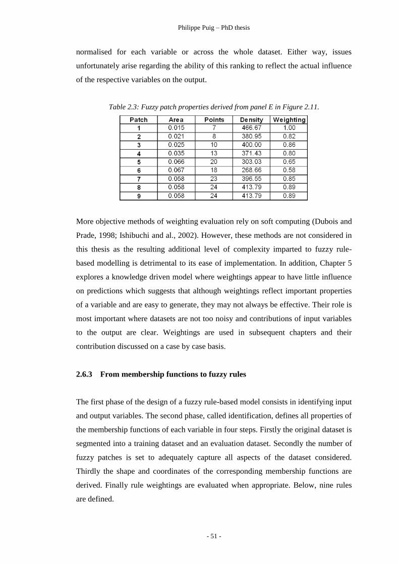
Philippe Puig – PhD thesis
- 51 -
normalised for each variable or across the whole dataset. Either way, issues
unfortunately arise regarding the ability of this ranking to reflect the actual influence
of the respective variables on the output.
Table 2.3: Fuzzy patch properties derived from panel E in Figure 2.11.
More objective methods of weighting evaluation rely on soft computing (Dubois and
Prade, 1998; Ishibuchi and al., 2002). However, these methods are not considered in
this thesis as the resulting additional level of complexity imparted to fuzzy rule-
based modelling is detrimental to its ease of implementation. In addition, Chapter 5
explores a knowledge driven model where weightings appear to have little influence
on predictions which suggests that although weightings reflect important properties
of a variable and are easy to generate, they may not always be effective. Their role is
most important where datasets are not too noisy and contributions of input variables
to the output are clear. Weightings are used in subsequent chapters and their
contribution discussed on a case by case basis.
2.6.3 From membership functions to fuzzy rules
The first phase of the design of a fuzzy rule-based model consists in identifying input
and output variables. The second phase, called identification, defines all properties of
the membership functions of each variable in four steps. Firstly the original dataset is
segmented into a training dataset and an evaluation dataset. Secondly the number of
fuzzy patches is set to adequately capture all aspects of the dataset considered.
Thirdly the shape and coordinates of the corresponding membership functions are
derived. Finally rule weightings are evaluated when appropriate. Below, nine rules
are defined.

Philippe Puig – PhD thesis
- 52 -
Rule 1 IF Input MF 1 THEN Output MF 1 Weighting = 1
Rule 2 IF Input MF 2 THEN Output MF 2 Weighting = 0.82
Rule 3 IF Input MF 3 THEN Output MF 3 Weighting = 0.86
Rule 4 IF Input MF 4 THEN Output MF 4 Weighting = 0.80
Rule 5 IF Input MF 5 THEN Output MF 5 Weighting = 0.65
Rule 6 IF Input MF 6 THEN Output MF 6 Weighting = 0.58
Rule 7 IF Input MF 7 THEN Output MF 7 Weighting = 0.85
Rule 8 IF Input MF 8 THEN Output MF 8 Weighting = 0.89
Rule 9 IF Input MF 9 THEN Output MF 9 Weighting = 0.89
The above set of rules defines how fuzzy antecedents relate to fuzzy consequents.
The next section details the functions of a fuzzy model which turn these fuzzy rules
into a predictive framework.
2.7 Structure and functions of a fuzzy rule-based model
An abundant literature on fuzzy rule based-modelling (Dubois and Prade, 1996),
ranging from superficial but practical (Von Altrock, 1995) to advanced (Kandel,
1986), is not always relevant to the intent of this thesis, which is to simplify GIS
modelling by providing a unified predictive framework in GIS modelling. Four
sources of information were very influential in shaping sections of this chapter and
the overall fuzzy rule-based modelling strategy detailed in this thesis. Bardossy and
Duckstein (1995) provide a complete and readable coverage of applied fuzzy-rule
based modelling. Klir and Bo Yuan (1995) offer an excellent background on a wide
range of aspects of fuzzy logic and fuzzy modelling. Babuska‟s (1996) study of
fundamental differences between Mamdani and Takagi-Sugeno type fuzzy rule-
based models contains clear and in depth coverage of important technical issues. Cox
(1999) focuses on practical aspects of the implementation of fuzzy rule-based models.
Research in alternative interpretations of fuzzy rules (Shepard, 2005; Jones et al.,
2009) reveals an interesting evolution of fuzzy rule-based systems. While Shepard
(2005) describes fuzzy rule-based systems in perfect agreement with previous
references, Jones et al. (2009) reflect in their work the growing interest in fuzzy rule-

Philippe Puig – PhD thesis
- 53 -
based systems of gradual implicative rules. These systems are not considered in this
thesis as they do not have many applications yet. However, since they lead to a
different type of knowledge representation (Jones et al., 2005) they may well provide
practical improvements to current fuzzy rule-based models.
Sections 2.7.1 to 2.7.6 of this Chapter rely on the sources of information cited above
to explore the structure of fuzzy rule-based models. The four functions of a fuzzy
rule-based model are in chronological order fuzzification, implication, aggregation
and defuzzification. The implementation and integration of these functional blocks
was initially explored in Excel (Kelly, 2006). A functional fuzzy rule-based
modelling application called EXFIS (Excel Fuzzy Inference System), described in
Appendix 1, was implemented. Detailed expressions for operators described in
sections 2.7.1 to 2.7.6, including rule weighting algorithms, can be found in
Appendix 1.
2.7.1 Diagrammatic representation of fundamental processes in a fuzzy rule-
based model
The diagram in Figure 2.12 refers to the Mamdani inference system (Babuska, 1996)
which represents the first practical implementation of Zadeh's (1965) principles of
fuzzy logic. Mamdani, who worked on the development of control systems in the
1970's at Queen Mary College in London, devised a fuzzy controller for cement kilns
built in the early 1980s. Mamdani‟s inference system is associated with the first
industrial implementation of fuzzy logic. Other models are not discussed in this
thesis as they have very few practical applications to natural systems and NRM.
These include the singleton model, the fuzzy relational model and the Takagi-Sugeno
(TS) model (Babuska, 1996). The TS inference system is very popular in engineering
where the general shape of the output is often known. The output of natural systems
can rarely be represented by a simple mathematical expression. Mamdani type
inference systems do not require predefined output mathematical expression. What
follows focuses therefore on Mamdani type inference systems which are better suited
to GIS modelling. Adding membership degrees to the conclusion, as depicted in
Figure 12.2, however is to be attributed to Kosko (1994), as Mamdani and Assilian

Philippe Puig – PhD thesis
- 54 -
(1975) used maximum instead of sum and centroid defuzzification to evaluate the
output in Figure 2.12.
Figure 2.12: Succession of processes in the development of a fuzzy rule-based model, also
called Fuzzy Inference System (FIS). There are only 2 rules defined by 4 membership
functions. The Output is 25.36 and the Input vector (4.5, 43.4).
Figure 2.12 is the diagrammatic representation of a simple fuzzy rule-based model
with multiple inputs and a single output (MISO). This type of model can be
considered as the fundamental building block of fuzzy rule-based predictive models.
All membership functions of the model in Figure 2.12 are triangular. Only two rules
fired by the input value are displayed in this model. Four sequential tasks are
successively completed by four separate operators. Rule 2 carries a higher weighting
than rule 1 as a result of decisions made during the identification process. The
prediction of this model for the input vector (4.8, 43.4) is 25.4. The Degree of
Fulfilment of Rule (DOF) is the level to which a rule applies. This degree is
measured by the membership of the input value in the antecedent membership
function of the corresponding rule. In this model, the value 4.8 fires Rule 1 to only
60% of its maximum effect and its DOF is therefore 0.6. The value 43.4 fires Rule 2
at only 20% of its maximum capacity: rule 2 has a DOF of only 0.2. As they are only
partially fired they are vertically rescaled in proportion. These results are combined
through the graphical addition of the two membership functions. The output
therefore is a shape which grows in size with the number of rules fired. The answer

Philippe Puig – PhD thesis
- 55 -
remains vague and needs to be defuzzified if it has to have any practical application.
The defuzzified result is the single value which accounts best for the respective
contribution of all rules fired. Here the centre of gravity (COG) is the defuzzification
method used. It consists in projecting the centre of gravity of the sum of all rule
membership functions, modified by their DOF and weighting, on the horizontal axis,
as the clustering of the output variables is generally imposed on the input variables
(Bilgic and Turksen, 2000: p.215). This position corresponds to the x coordinate of
the largest combined contributions of all fired rules to the final result. Here the final
output of the model is 25.36.
The model in Figure 2.12 has only two variables and only two rules are fired. In
reality a minimum of two rules are frequently fired in each variable as a result of
membership functions overlap. Real models generally have a minimum of three rules
per variable. The model in Figure 2.12 is a MISO model. A combination of MISO
models can achieve the same outcome as any multiple input multiple output (MIMO)
model. The resulting model is less compact but more transparent. MISO high
dimensionality predictive models are more readable and are therefore preferred in
this thesis. Natural systems are typically described by a large number of parameters
in addition to geographical dimensions. The architecture of fuzzy rule based models
and their ability to tackle high dimensionality problems is consequently well suited
to predictive modelling applications for natural resources management in a GIS
environment.
2.7.2 Fuzzy rule-based modelling operations
The four steps of processing in a fuzzy rule-based model, displayed in Figure 2.12,
rely on algebraic operations that need to be defined. These operations often lead to a
great deal of confusion. Venn diagrams provide the basis for the definition of the two
fundamental operations on sets called union and intersection. Union and intersection
are operations on sets similar to addition and multiplication on real numbers,
respectively. This however, casts little light on the algebraic expression used to
evaluate the following fuzzy logic statement.
V1_MF1(0.5) AND V2_MF2(23)

Philippe Puig – PhD thesis
- 56 -
In other words, how do we algebraically express AND/multiplication and
OR/addition to perform operation(s) on degrees of membership? A number of texts
(Kandel, 1986; Terano et al., 1992; Bouchon-Meunier, 1993; Bardossy and
Duckstein, 1995) provide in depth discussions of theoretical considerations leading
to the choice of fuzzy operators available. The last reference is probably the most
relevant to our needs. Bardossy and Duckstein (1995) give a concise and clear
justification of the unusual variety of pairs of operators playing in fuzzy logic roles
equivalent to those of addition and multiplication on real numbers. Firstly, the
problem consists of finding practical mathematical expressions of addition and
multiplication on membership functions that have all the desirable theoretical set
properties. Secondly, these expressions need to be mathematically tractable. Thirdly,
they need to make sense when applied to real problems. The fuzzy logic literature
offers many operations which can perform the four steps in Figure 2.12.
Only some of the operations described in the literature are available in the fuzzy
modelling software used in this thesis. Brief discussions of some theoretic aspects of
fuzzy logic are necessary for two reasons. Firstly, fuzzy modelling is often dismissed
(Dubois and Prade, 1994; Cox, 1999) by proponents of alternative mathematical
models of vagueness who do not share the same scientific background (Dubois and
Prade, 1993: p.1059). They fail, for instance to appreciate the synergy of merging
statistical and fuzzy modelling to simultaneously address both uncertainty and
imprecision as explained in Chapter 1. Secondly, a software like Matlab and Scilab,
used to construct and evaluate fuzzy models, requires to make a number of choices
including t-norm and t-conorm, implication and aggregation operators as well as
defuzzification methods. The following sections are therefore necessary for the
implementation fuzzy rule-based models discussed in Chapters 4 and 5.
2.7.3 t-norm (fuzzy intersection) and t-conorm (fuzzy union) operators
As mentioned earlier, familiar algebraic addition and multiplication do not apply to
sets. Union and intersection are their equivalent in set theory. Union and intersection,
are readily compatible with logic operators OR and AND used to combine

Philippe Puig – PhD thesis
- 57 -
membership functions. They do not however apply to membership values contributed
by the respective antecedent membership functions in the rule below.
IF Input1 AND Input2 OR Input3 THEN Output1
In the context of fuzzy rule-based modelling, logical operators AND and OR are
assigned algebraic expressions called t-norm, or fuzzy intersection, and t-conorm or
fuzzy union ((Klir and Bo Yuan, 1995: p.62). Algebraic expressions generally need
to satisfy at least the four conditions of commutativity, associativity, monotonicity
and idempotency. Among all possible contenders, only a small number of algebraic
expressions meet these four conditions and lead to meaningful results when applied
to the physical world. The first pair of t-norm and t-conorm operators proposed by
Zadeh (1965) were the minimum and maximum functions. Below is a brief
discussion of some practical implementations of t-norm and t-conorm operators.
Once a t-norm (multiplication like operator) has been selected, the t-conorm
(addition like operator) is fixed as they are mathematically linked by the two
equations below where c and t respectively represent t-conorm and t-norm.
t(x,y) = 1-c(1-x, 1-y) Equation 2.3
c(x,y) = 1-t(1-x, 1-y) Equation 2.4
Researchers strived to propose t and c expressions with realistic outcomes. Among
them, Yager, Dubois and Prade (Klir and Bo Yuan, 1995: p.74, p. 82) proposed
suitable expressions meeting the conditions defined in Equations 2.3 and 2.4.
Bardossy and Duckstein (1995) consider t-norms and t-conorms performance within
the context of fuzzy rule-based modelling applied to geophysical, biological and
engineering systems. They propose a short list of 5 norm conorm pairs (Bardossy and
Duckstein, 1995: p.13). The choice of norm conorm pair reflects the type of
application as well as the modeller‟s preference. Bardossy and Duckstein (1995)
prefer the product-sum defined by the two equations below where x and y are
membership values.
t(x,y): x AND y = xy Equation 2.5

Philippe Puig – PhD thesis
- 58 -
c(x,y): x OR y = x + y – xy Equation 2.6
In addition to being mathematically simpler than alternative expressions, the
algebraic product-sum is supported in Matlab and Scilab, both used in case studies
discussed in this thesis. The algebraic product-sum is therefore the (norm, conorm)
pair used in this thesis.
2.7.4 Implication: degree of fulfilment of a rule (DOF) and product inference
The level of truth of IF …THEN statements is called the degree of fulfilment (DOF)
of the corresponding rule. Fuzzy rule-based modelling does not directly deal with
fuzzy sets but with the membership values of elements in fuzzy sets which ultimately
dictate the DOFs of all rules of the model. Figure 2.12 shows simple logical
statements lead to straightforward DOF calculations. One fundamental concern is
therefore the evaluation of the level of truth of a logical statement combining at least
two antecedent variables.
IF Hot AND Humid OR Dusty THEN Uncomfortable
The antecedent premise above, like those displayed in Figure 2.12, does not
necessarily combine multiple fuzzy sets such as „Hot‟ and „Humid‟ in the rule above.
Data driven models rarely do as they generally rely on direct associations between
input and output variables while knowledge driven models, on the contrary, often do
as they replicate logical associations between multiple causes and effects common in
human languages. Mathematical expressions are therefore required to evaluate the
level of truth of the above logical statement from the DOFs of antecedent premises.
Bardossy and Duckstein (1995) offer clear guidelines to evaluate the DOF of the
statement above for all possible combinations of antecedent premises. Following
their terminology, the Greek letter is the symbol used for DOF. Let us assume that
we are interested in evaluating logical statements involving the memberships A1(a1)
and A2(a2) of elements a1 and a2 in fuzzy sets A1 and A2. We need to translate, into
an algebraic expression, the DOF of fundamental logical operators AND, OR, NOT,

Philippe Puig – PhD thesis
- 59 -
XOR. Based on product-sum expressions in Equations 2.5 and 2.6, the following
expressions are proposed.
( A1) = A1(a1)
( NOT A1) = 1 - A1(a1)
( A1 AND A2) = A1(a1). A2(a2) Equation group 2.7
( A1 OR A2) = A1(a1) + A2(a2) - A1(a1). A2(a2)
( A1 XOR A2) = A1(a1) + A2(a2) - 2 A1(a1). A2(a2)
The algebraic expression of an antecedent with any combination of the 4 logical
operators above can be derived from Equation group 2.7 above. In addition to these
familiar logical operators, Bardossy and Duckstein (1995) offer additional operators
such as MOST OF THE PROPOSITIONS and at AT LEAST A FEW that play
important roles in special applications of fuzzy logic such as the control of traffic
lights. These belong to a group of linguistic expressions, called hedges, which
include linguistic terms such as MORE, SLIGHTLY, etc. They modulate
fundamental linguistic terms such as GOOD, BAD. A number of mathematical
definitions have been proposed (Bardossy and Duckstein, 1995: p. 15) for a variety
of hedges. Their objectivity, however, appears questionable. They may play a useful
role in knowledge modelling but it seems difficult to ascertain that informants agree
with the way „hedges‟ modify the information they contribute. Hedges are not
considered in this thesis as I believe that they would add an unnecessary level of
subjectivity detrimental to the overall transparency of the final model.
Applications considered in this dissertation do not require complicated logical
combinations of antecedents, and nor does the complete fuzzy rule-based expert
system of Cheung et al. (2005) described in Chapter 5. In all examples considered in
this thesis, data as well as knowledge driven fuzzy rule-based models can be
exclusively built from rules associating a single antecedent membership function to a
single consequent membership function. If this approach is unsuitable, equations in
this section enable the derivation of appropriate algebraic expressions suited to the
most complicated logical statements. Simple and short fuzzy rules remain one of the
most desirable features of a good fuzzy rule-based model. Increasing the number of

Philippe Puig – PhD thesis
- 60 -
rules appears to be a better option than increasing their complexity. Transparency
and simplicity guide models discussed in this thesis.
2.7.5 The role of implication in fuzzy rules
Implication consists in reflecting the DOF of a rule in the output membership
function of this rule. The implication operator THEN thus transfers the DOF of the
antecedent which can be, as discussed in the previous section, either a single
membership function or a series of membership functions linked by logical operators.
The DOF of the output membership function, as shown in Figure 2.12, rescales the
output membership function. Practically this rescaling is achieved, in triangular
fuzzy number for instance, by multiplying the central value by the DOF. A triangular
output membership function of a rule whose antecedent has a DOF of 0.5 is therefore
only half of its maximum height of 1. For a DOF of 0 the output membership
function has a height of 0. Consequently the corresponding rule is not expressed. A
DOF of 1, on the contrary, means that the output membership function has its
maximum size and is therefore fully expressed. The implication process therefore
modifies the height of the output membership function, and therefore its centre of
gravity.
2.7.6 Rule combination
Bardossy and Duckstein (1995) outline three important properties of rule
combination. The first property, idempotence, ensures that a rule can be combined
with itself without changing its outcome. The second and third properties,
associativity and symmetry, are necessary to ensure that rules can be combined in
any order. Out of all possible rule aggregation methods the most commonly used are
minimum, maximum and addition. The latter is often preferred because all rule
contributions are incorporated. Minimum and maximum, on the contrary, fail to
account for repeated consequences. This lack of sensitivity to smaller individual
contributions, even if they occur in large number, amounts to a loss of information.
The sum combination does not suffer from this limitation and can be weighted as
well while weightings clearly play no role in minimum or maximum aggregation
methods. There are good reasons to explore in detail aggregation methods and the

Philippe Puig – PhD thesis
- 61 -
type of logical operator used. The Combs method (Cox, 1999) for instance addresses
the combinatorial rule explosion problem by a clever replacement of AND by OR.
This thesis however steers away from such advanced concepts to provide a robust
and simple approach to the development of rule-based models.
2.7.7 Defuzzification
The output of a Mamdani type fuzzy model (Mathworks, 1995) is the graphic sum of
individual membership function polygons contributed by each rule of the fuzzy rule-
based model. The output is therefore a polygon positioned within the range of output
values. This polygon provides, through its size, shape and position on the output axis,
a vague indication of what the corresponding output value should be. Defuzzification
transforms this polygon into a number. Defuzzification, contrary to other facets of
fuzzy rule based modelling does not appear to be supported by a robust theoretical
framework. Cox (1999: p 31) stresses that defuzzification methods are not derived
from fuzzy theory. They are merely acceptable empirical recipes to translate the
position of a polygon on a horizontal axis into a single number. Justifications for the
different methods proposed are directly linked to the performance of the model. As
performance is a compromise between efficiency and accuracy, algorithms preferred
in the 1970s, such as maximum, were largely driven by computational constraints of
the time. However, since the 1970s, due to a remarkable evolution of information
technology, the overall best algorithms can now be adopted instead. The three most
popular methods of defuzzification (Klir and Bo Yuan, 1995; Babuska, 1996; Cox,
1999; Bardossy and Duckstein, 1995) are the centre of area, also called centre of
gravity (COG), the mean of maxima (MOM) and the maximum. COG and MOM are
compared in Figure 2.13. Although results are close, MOM prediction only changes
if the maximum rule value changes.
COG is more sensitive as any modification of grey triangles in Figure 2.13 will affect
the COG position and therefore model prediction. COG is generally preferred as it
combines, contrary to maximum, the output of all rules. Furthermore COG is part of
the methodology described by Kosko (1994) in his seminal paper on fuzzy rule-
based systems as universal approximators. COG is the defuzzification method used
in all applications described in this thesis. Well supported by both Matlab and Scilab

Philippe Puig – PhD thesis
- 62 -
fuzzy toolboxes, the underlying principle is intuitively more acceptable than any
value read from the position of local maxima or minima.
Figure 2.13: Comparison of two defuzzification methods - Centre of gravity (COG) on the
left and mean of maxima (MOM) on the right. Rule outputs of the fuzzy rule-based model are
the three grey triangles. The overall output of the model is the dark grey polygon obtained by
adding up the three light grey triangles.
2.8 Implementation of a fuzzy rule-based model
The fuzzy rule-based strategy detailed in section 2.7 is applied to the problem
defined in section 2.6. Fuzzy rule-based modelling is computationally demanding
and therefore relies heavily on specialist software. Five different pieces of software
were used to build the models described in this thesis.
ArcView 3.2 (Lee and Wong, 2001), with various extensions, is the only GIS
software used in this thesis. The role of ArcView 3.2 is described in Chapter 3 and
Appendix 3. Fuzme (Minasny and McBratney, 2002), a clustering freeware created
at Sydney University, provided the segmentation capability required in Chapter 4.
Excel (Kelly, 2006) was used to develop a fuzzy rule-based modelling environment
detailed in Appendix 1. This proved to be a very useful training environment. Matlab
(MathWorks, 1999) and Scilab (Campbell et al., 2006) are the applications most
fuzzy rule-based models described here were built in. Scilab is a free Matlab clone.
A step by step implementation of fuzzy models in Scilab is presented in Appendix 4.

Philippe Puig – PhD thesis
- 63 -
The problem defined in section 2.6 is solved in Scilab using sciFLT (Urzua, 2004),
the Scilab Fuzzy Logic Toolbox.
2.8.1 Model implementation in Scilab
Figure 2.14 to 2.17 visualise all information described in section 2.7 that need to be
entered in Scilab to build the model in Figure 2.11.
Figure 2.14: Screenshot of fls Editor of sciFLT showing the Description panel where the
type of model and its parameters can be easily selected.
The Description panel, in Figure 2.14 above, enables the selection of suitable
parameters including t-norm and t-conorm pairs, implication, aggregation and
defuzzification operators to completely describe the Mamdani type fuzzy rule-based
model required. Although there is little doubt that some combinations perform better
in some specific contexts, the selection of operators displayed in this panel was used
in all applications considered in this thesis.

Philippe Puig – PhD thesis
- 64 -
Figure 2.15: Screenshot of fls Editor of sciFLT showing the Rule definition panel where the
type of membership, its parameters and the name of the corresponding rule are entered.
Figure 2.15 shows the nine membership functions (X1 to X9) of X, the only input
variable in this model. The scilab toolbox sciFLT offers several membership function
types. The type selected here is “trimf” which stands for triangular membership
function. Once the type is selected the range of values covered, [0,0.94] in this case,
and the coordinates of the three apices of each membership function are entered in
the column under “par” for parameters. The same procedure is adopted to define the
Y output variable. All input and output membership functions parameters are entered
as shown in Figure 2.15. The model requires five operators to be defined from the
sciFLT window in Figure 2.14. The algebraic sum and algebraic product for the
(norm, conorm) pair are picked from the „S-Norm Class‟ group and „T-Norm Class‟
groups respectively. One is selected from „Complement‟ for the maximum
membership value. The „Implication Method‟ is set to product. Sum is the
„Aggregation Method‟. Finally centroid (COG) is selected for the „Defuzzification

Philippe Puig – PhD thesis
- 65 -
Method‟. Most default settings are kept with exception of the aggregation method
which is Maximum by default.
Figure 2.16: Screenshot of fls Editor of sciFLT showing the Rule definition panel where
membership functions defined in Figure 2.15 are embedded in rules.
All possible associations between input and output membership functions defined by the
fuzzy model are expressed as rules. This model is completely defined by nine rules displayed
by the fuzzy logic system (fls) editor in Figure 2.16. All rules have the same default
weighting 1. Figure 2.17 summarises this model as Mamdani (m) type model with 1
input, 1 output and 9 rules.
Figure 2.17: Screenshot of fls Editor of sciFLT showing a summary of the characteristic
features of this universal approximator model.

Philippe Puig – PhD thesis
- 66 -
2.8.2 Model evaluation
Figure 2.18 compares the values of the evaluation dataset, represented by circles in
panel F of Figure 2.11, with model predictions based on the x coordinates of these
records. The cloud of points is well aligned on the diagonal through the origin. This
first impression is confirmed by the high correlation coefficient is 0.964. Any
improvement on this model would require additional time and effort which a
cost/benefit analysis may show to be unwarranted within that context. The dataset
considered, like most real NRM datasets, contains a stochastic component that no
model can replicate, thus making a correlation coefficient of 1 beyond the reach of
models of natural systems. The model once completed is still a fuzzy rule-based
model. It does not have an equivalent algebraic expression. Outputs, however, can
then be fed into algebraic expressions downstream from the modelling process.
Figure 2.18: Model predictions plotted against experimental values.
The performance of the model is assessed by plotting, in Figure 2.18, the model
predictions against experimental values. Although not forming a perfect straight line
at 45 degrees gradient through the origin, this plot is representative of a good
predictive model.

Philippe Puig – PhD thesis
- 67 -
Summary
Predictive models are classified as white, grey or black box type. Owing to the direct
association between rules and modelled processes, the transparency of fuzzy rule-
based models puts them in the grey box category. Membership functions, a key
component of fuzzy models, play a crucial role in making rules highly readable
particularly when linguistic terms are used. A comparison of Boolean and fuzzy logic
sheds some light on the contribution of membership functions to an improved
description of natural processes. Membership functions allow fuzzy predictive
models, unlike their Boolean counterparts, to be built from the very linguistic terms
humans naturally rely on in their predictive reasoning. The versatility of
membership functions comes at a price. There are many designs to choose from.
Fortunately the simplest of all, the triangular membership is the most widely used as
it performs well in most situations.
Much as been written about the statistical nature of membership functions as fuzzy
and statistical representation of uncertainty have often been pitted against each other.
Although Zadeh (1965) initially declared the concept of membership function to be
non statistical, Dubois and Prade (1993) consider that the issue is multifaceted.
Regardless of the controversy, membership functions offer real advantages in the
GIS representation of geographic entities. These encompass a variety of sources of
uncertainty better accounted for by a combination of statistics and fuzzy logic than
by statistics alone. Although membership functions are particularly well suited to the
representation of the linguistic terms, they are equally well suited to stochastic
uncertainty. Owing to the importance of their role, the acquisition of membership
function deserves some attention. Kosko‟s (1994) concept of fuzzy patches and
universal approximator is widely implemented in this thesis. Fuzzy patches are
graphical visualisations of the fuzzy association between input and output data. They
provide a generic framework for membership function design, thus a universal
technique to make predictions on the basis of observations and therefore to predictive
modelling. The method is articulated around three processes which are in
chronological order: identification, implementation and evaluation.

Philippe Puig – PhD thesis
- 68 -
Identification is concerned with the definition of all components of the model. Input
and output variables are all translated into membership functions. Parameters
describing each membership functions are calculated. Rules and their corresponding
weightings, if necessary, are directly derived from associations observed in the
training dataset between input and output data.
Implementation consists in applying the fuzzy rule-based model previously defined
to input data. Four successive processes are involved: fuzzification, implication,
aggregation and defuzzification. These steps are better summarised diagrammatically
as a flowchart. A range of possible mathematical operators is available to perform
each of the four processes. Although both Takagi-Sugeno and Mamdani fuzzy rule-
based models are widely used, only the latter is considered in this thesis. The
implementation is computationally demanding and therefore relies on purpose built
software. Scilab fuzzy logic toolbox is the main software used in case studies of this
thesis.
Evaluation consists in assessing the performance of the model by comparing
predictions and actual values. The evaluation metric used in this thesis is the
correlation coefficient between observations and model predictions. This familiar
metric confirms that, in the case study considered in this chapter, the fuzzy rule-
based model created has very good predictive capabilities. Its correlation coefficient
of 0.96 is very close to 1 which corresponds to a perfect model.

CHAPTER 3
GIS FUZZY MULTICRITERIA DECISION ANALYSIS
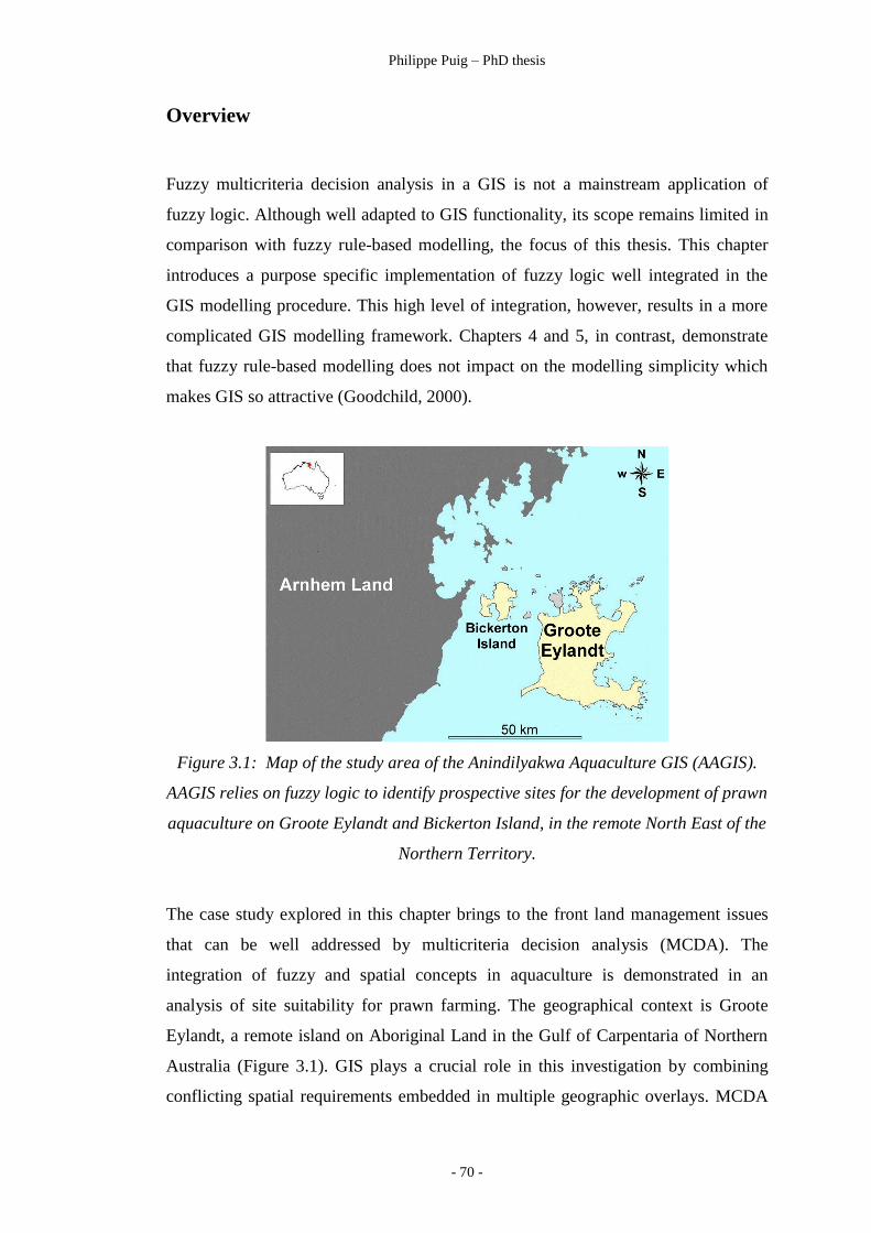
Philippe Puig – PhD thesis
- 70 -
Overview
Fuzzy multicriteria decision analysis in a GIS is not a mainstream application of
fuzzy logic. Although well adapted to GIS functionality, its scope remains limited in
comparison with fuzzy rule-based modelling, the focus of this thesis. This chapter
introduces a purpose specific implementation of fuzzy logic well integrated in the
GIS modelling procedure. This high level of integration, however, results in a more
complicated GIS modelling framework. Chapters 4 and 5, in contrast, demonstrate
that fuzzy rule-based modelling does not impact on the modelling simplicity which
makes GIS so attractive (Goodchild, 2000).
Figure 3.1: Map of the study area of the Anindilyakwa Aquaculture GIS (AAGIS).
AAGIS relies on fuzzy logic to identify prospective sites for the development of prawn
aquaculture on Groote Eylandt and Bickerton Island, in the remote North East of the
Northern Territory.
The case study explored in this chapter brings to the front land management issues
that can be well addressed by multicriteria decision analysis (MCDA). The
integration of fuzzy and spatial concepts in aquaculture is demonstrated in an
analysis of site suitability for prawn farming. The geographical context is Groote
Eylandt, a remote island on Aboriginal Land in the Gulf of Carpentaria of Northern
Australia (Figure 3.1). GIS plays a crucial role in this investigation by combining
conflicting spatial requirements embedded in multiple geographic overlays. MCDA

Philippe Puig – PhD thesis
- 71 -
in this case study relies on Saaty’s analytic hierarchy process (AHP) used in many
domains including management (Saaty, 1982) and GIS (Eastman, 2009). The
principles of AHP, merely mentioned in Chapter 3, are detailed in the literature
(Saaty, 2001).
The main role of fuzzy logic in this case study is to facilitate the definition of
suitability rankings applied to the different classes of criteria considered. Linguistic
terms are used instead of more abstract numerical values thus facilitating the merging
of specialist knowledge with environmental data. The visualisation of spatial
uncertainty introduced in section 2.4.2 offers an unusual geographic summary of all
vague information considered.
Mapping fuzziness as four separate interpretations of each linguistic term of
suitability is the most conspicuous characteristic of this approach (Puig, 2001). In the
process of generating these maps, the fuzzy technique adopted better accounts for the
uncertainty inherent in site selection by providing visual representations of the range
of meanings implied by linguistic terms. Constraints, criteria, ranks and weightings
can all be expressed in linguistic, non-technical terms more accessible to lay persons
than mathematical expressions. Although the approach may appear complicated,
underlying processes rely on simple mathematical operations known as grid algebra.
All leading professional GIS software offer the same essential functionality required
by grid algebra (DeMers, 1997) extensively used in the Anindilyakwa Aquaculture
GIS (AAGIS) (Puig, 2008). Wherever a grid is laid over a variable defined across a
plane, values of the variable transferred to the corresponding grid cells can be
combined with other values, in the same location in other grids, by using algebraic
expressions. A raster representation of geographic entities is therefore very
convenient as it addresses fundamental needs. Changes in values of a mapped
variable can be displayed in grid format to facilitate the conceptualisation of complex
underlying processes. Grid algebra adapts the technique of transparency overlays to
GIS. Mathematical operations, required to provide the rigour attached to complex
geographical reasoning, become readily available through the GIS. Through grid
algebra, all fuzzy logic based models discussed in subsequent chapters are all directly
relevant to GIS modelling.
Philippe Puig – PhD thesis
- 72 -
3.1 Background
As a professional Spatial Scientist, I completed commercial projects pertinent to this
thesis. Below is a case study adapted from an investigation I carried out for the
Government of the Northern Territory of Australia.
This case study explores scientific aspects of a commercial GIS project, focused on
some remote islands of Northern Australia. This case study is taken from a project
commissioned by the Northern Territory Department of Fisheries. The GIS solution
had to reflect the specificity of the location. The aim was to provide Aboriginal
traditional owners with an incentive to prompt the business sector into investigating
the potential of aquaculture on Aboriginal Land. This aquaculture GIS had to be fully
capable of merging Aboriginal and Western knowledge into one single output.
These knowledges differ in many ways. The former is qualitative, holistic, timeless
and oral (Malloch, 1989; Smith and Marsh, 1990; Chaloupka, 1993; Castellano, 2000)
while the latter is quantitative, reductionist, short-term and written (Tsuji and Ho,
2002). This project intended only to address the last difference. Interfacing with
knowledge and linguistic differences was therefore crucial. Fuzzy logic is well suited
to translate human knowledge into quantitative models. Issues of culture and
therefore language are distinctive features of Aboriginal land. Fuzzy logic therefore
became a key feature of this project.
3.1.1 Purpose of the project
The project consisted of GIS identification of the best prawn farming sites on the
coasts of Groote Eylandt and Bickerton Island displayed in Figure 3.1. The outcome
of this GIS desktop study was to map environmental variables considered to be
crucial for prawn farming. Once prime locations are identified field surveys need to
be carried out by interested developers to confirm suitability. The purpose of the
GIS investigation is therefore to limit fieldwork to the most promising locations. The
GIS approach minimises the high cost of feasibility studies in such remote locations.

Philippe Puig – PhD thesis
- 73 -
3.1.2 A unique geographical and cultural context
The Anindilyakwa Aquaculture GIS, named after the local Aboriginal Council,
provides a site suitability analysis designed to facilitate the identification of potential
aquaculture sites. This low cost management tool is well suited to aquaculture
development at local, regional and national scales. The GIS handles tedious and time
consuming tasks while aquaculture specialists concentrate on the identification of
physical and economical constraints including the assessment of their relative
importance. Owing mainly to the abundance of rocky outcrops, ongoing mining
activity and seasonal weather patterns, nearly 3/4 of the area of interest is unsuitable
for aquaculture. The most promising locations are concentrated in the south of
Bickerton Island and Groote Eylandt.
Few interpretative environmental maps of this area exist. Maps of aquaculture
suitability produced by the GIS are therefore an important element in the
development of integrated coastal management plans. An inventory of aquaculture
sites in the Northern Territory is part of the Government’s strategic approach to
aquaculture development. AAGIS represented a deliberate effort to improve
technical communication with indigenous stake holders. Explanations to traditional
owners were greatly facilitated by the reliance on visual information readily available
from the GIS.
3.2 Method and data
The AAGIS is articulated around the effective mapping of prawn aquaculture site
suitability based on environmental data and expert knowledge. First the method
adopted to map the fuzzy suitability derived from the available information is
outlined. Then the dataset used in this study is described. Finally the technique used
to capture knowledge of the two aquaculture experts who steered this project is
investigated. Complementary information related to the source of the data and other
technical issues is available in Appendix 2.

Philippe Puig – PhD thesis
- 74 -
3.2.1 Mapping fuzziness
Mapping areas of high potential for prawn farming consisted first of excluding
unsuitable locations. Mangroves, sacred sites, mining infrastructure and their
immediate surrounding, fall in that category. Aquaculture experts involved in this
project then identified suitability criteria including slope, access, proximity of
infrastructure, distance to the coast, soil depth, ground water availability,
susceptibility to flooding. Each criterion is initially represented as a vector layer.
Here, the GIS representation relies both on AHP and fuzzy logic. This approach
introduced by Banai (1993) was subsequently adopted by other researchers (Gemitzi
et al., 2006; Vahidnia et al., 2008; Farzanmanesh, 2010). This duality may explain
why, although concise, this thematic mapping described in this thesis does not
translate into simple mathematical procedures. However, the combination of AHP,
fuzzy logic and GIS, widely used in natural resource management (Mc Bratney and
Odeh, 1997; Schmoldt et al., 2001; Chang et al., 2008) has been successfully
implemented in IDRISI (Eastman, 2009), one of the most sophisticated commercial
raster based GIS software.
The GIS implementation of the method described in this chapter requires translating
the various vector maps of environmental criteria described in Appendix 2 into grids.
Suitability, defined by aquaculture experts in linguistic terms, is fuzzified for each
criterion into 4 grids (a,b,c,d) as displayed in Figure 2.7. All 4 grids, for each
criterion, are assigned the same weighting estimated by pair wise comparisons of all
suitability criteria performed by the aquaculture experts. All weighted grids of type a
are then added to produce a final grid of suitability A. Final grids B, C and D are
similarly generated. Although the 4 maps carry crucial information, a single
summary capable of guiding field investigations is required. Defuzzification plays
this role.
Defuzzification is performed, in this case by adding maps A, B, C and D, as
recommended by Malczewski (1999). However, only zones where the highest
suitability persists across the four grids A, B, C and D were considered. In addition,
aquaculture experts required areas covering no less than 1 ha. All prime targets for

Philippe Puig – PhD thesis
- 75 -
future investigation therefore display the highest suitability across the four maps and
cover no less than 1ha of contiguous grid cells.
3.2.2 Source data
This site suitability analysis is based on variables listed in Table 3.1. These variables
were derived from the digital datasets in Table 3.2
Table3.1: Source data sets of AAGIS.
Source data and suitability criteria, although explored in Appendix 2, are listed here
to stress the high variability of the type of information and format used in this GIS
fuzzy model. A systematically high level of uncertainty is generally associated with
GIS modeling for two reasons. Firstly data in vector and raster formats are often
combined resulting in additional errors with each format change. Secondly
differences in scale imply that the nominal scale of the final product is downgraded
to that of the poorest dataset resolution used.
Table 3.2: Site selection criteria used to assess the suitability of a site for prawn aquaculture.
Knowledge capture, based on existing datasets listed in Appendix 2, is the most
important phase of development of the AAGIS. This 3 step process comprises the

Philippe Puig – PhD thesis
- 76 -
identification of suitability criteria, the evaluation of criteria weightings and the
definition by two DAC experts of ranges of suitability for all 10 criteria listed in
Table 3.2. The resulting model therefore captures expert knowledge through three
processes: environmental variables selection, weightings and translation of each
variable to membership functions. Complementary information on the source of the
data and other technical issues are available in Appendix 2.
3.2.3 Capture of knowledge derived from pair wise comparisons
Weightings are a key component of the expert knowledge captured in this model.
They summarise the knowledge embedded in pair wise comparisons. DAC experts
stressed that all criteria included in the model do not have the same importance.
Evaluating the relative importance of each criterion is difficult because experts with
different backgrounds have different views. The AHP (Saaty, 2001), well suited to
decision making (Saaty, 1990) and natural resource management (Schmoldt et al.,
2001) provides an appropriate knowledge acquisition framework in this case study.
Views expressed by DAC experts during the project are summarised in the relative
importance of site selection criteria listed in Table 3.3. These highlight the
importance of facilitating strategies to ensure the effective cooperation of those
involved. After working independently and obtaining conflicting weightings, the two
experts finally agreed to adopt a pair wise comparison method structured to ensure
maximum consistency. The importance of each suitability criterion is compared to
that of every other suitability criterion using the scale in Table 3.4. Values of relative
importance in Table 3.4 are all larger than 1 and the first criterion is always assumed
to be the most important. The order of the comparison between criteria is therefore
adjusted to always start with the most important of the two criteria. Alternatively the
inverse of values of relative importance can be used instead as demonstrated in Table
3.5. Each criterion is compared to the remaining criteria. Calculations of relative
importance for 5 criteria are demonstrated in Table 3.5.
Let us assume, using the terminology and values in Table 3.4, that we consider 5
hypothetical criteria C1 to C5. Their relative importance is defined in Table 3.3
below.

Philippe Puig – PhD thesis
- 77 -
Table 3.3: Relative importance of 5 criteria assessed by pair wise comparisons.
Pair wise comparison values are displayed in Table 3.5. Understanding these
calculations is important as they are the basis of weightings assigned to each criterion.
These weightings ultimately decide the level of suitability of a site for the
establishment of a prawn farm by taking into consideration all criteria in Table 3.2.
Table 3.4: Values of relative importance used in suitability criteria pair wise comparisons.
The evaluation of weightings is a tedious task handled semi automatically by a single
spreadsheet derived from that presented by Malczewski (1999). Experts start by
evaluating the relative importance of all selection criteria (C1 to C5 in Table 3.5)
identified. They fill in the green cells in Table 3.5 with a number read from Table 3.4.
Once two criteria Ci and Cj are compared, the spreadsheet automatically writes the
reciprocal value for the comparison of Cj and Ci in the appropriate cell below the
grey cells. All grey cells contain 1. They represent the importance of each criterion
relative to itself which is 1 according to Table 3.4. Criteria weightings (Malczewski,
1999: p.177) derived from pair wise comparisons are implemented in Table 3.6.
Values displayed in Table 3.6 are automatically calculated from numbers entered in
Table 3.5 for all weightings in blue cells. Details of calculations linking Tables 3.5,
3.6 and 3.7, as well as derivations of parameters listed below, are presented in
Appendix 2.4 as they require a description of spreadsheet formulas.

Philippe Puig – PhD thesis
- 78 -
The consistency of pair wise comparisons (Malczewski, 1999: p 184) is measured by
the Consistency Ratio (CR). CR is derived from λ and the Random Inconsistency (RI)
index. The eingenvalue associated with the principal eigenvector of the pair wise
comparison matrix (Eastman, 2009: p.138) is λ. Malczewski (1999: p.186) tabulated
values for RI for up to 15 criteria. A good approximation of CR is given by
Malczewski’s formula below:
RIn
nCR
)1(
Equation 3.1
Calculations of the CR (Malczewski, 1999, p. 186), and λ, the average value of the
consistency vector, are detailed in Appendix A 2.4. Saaty (1990: p.13) provides
additional information on the role of λ in assessing the consistency of the comparison
matrix including table in Table 3.5.
Malczewski (1999) states that CR values larger than 0.1 reflect inconsistent pair wise
comparisons. The following numerical demonstration helps understand the
importance of CR. The value of RI for 5 criteria (Malczewski, 1999: p. 186) is 1.12.
Based on calculations displayed in Tables 3.6 and 3.7, the consistency ratio for the
rankings of Table 3.5, using equation 3.1, is therefore:
638.012.1)15(5858.7
CR
There are therefore incompatible values of relative importance in Table 3.5. In this
example we can conclude that, because CR 0.1, weightings displayed in Table 3.6
are incorrect. Pair wise comparisons displayed in Table 3.5 need to be revisited until
CR < 0.1. In this instance there is at least one clear inconsistency in the three
leftmost green cells of Table 3.5: C1 cannot be more important than C2 and less
important than C3 while C2 is more important than C3. Although CR is useful in
checking the consistency of pair wise comparisons, maintaining CR below 0.1 is
virtually impossible as the number of criteria increases. With 55 pair wise
comparisons for 10 criteria, informants find it difficult to identify which pair wise
comparisons are contradictory. After a few attempts to bring CR below 0.1, they
retained the combination of relative importance ratings which minimizes CR. The
consistency ratio (CR), calculated from figures entered in Table 3.5, is derived from
the value of λ in Table 3.7. Using the method previously described, the two DAC
experts obtained the weightings in Table 3.8.
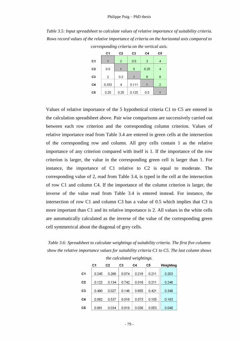
Philippe Puig – PhD thesis
- 79 -
Table 3.5: Input spreadsheet to calculate values of relative importance of suitability criteria.
Rows record values of the relative importance of criteria on the horizontal axis compared to
corresponding criteria on the vertical axis.
Values of relative importance of the 5 hypothetical criteria C1 to C5 are entered in
the calculation spreadsheet above. Pair wise comparisons are successively carried out
between each row criterion and the corresponding column criterion. Values of
relative importance read from Table 3.4 are entered in green cells at the intersection
of the corresponding row and column. All grey cells contain 1 as the relative
importance of any criterion compared with itself is 1. If the importance of the row
criterion is larger, the value in the corresponding green cell is larger than 1. For
instance, the importance of C1 relative to C2 is equal to moderate. The
corresponding value of 2, read from Table 3.4, is typed in the cell at the intersection
of row C1 and column C4. If the importance of the column criterion is larger, the
inverse of the value read from Table 3.4 is entered instead. For instance, the
intersection of row C1 and column C3 has a value of 0.5 which implies that C3 is
more important than C1 and its relative importance is 2. All values in the white cells
are automatically calculated as the inverse of the value of the corresponding green
cell symmetrical about the diagonal of grey cells.
Table 3.6: Spreadsheet to calculate weightings of suitability criteria. The first five columns
show the relative importance values for suitability criteria C1 to C5. The last column shows
the calculated weightings.

Philippe Puig – PhD thesis
- 80 -
The value of relative importance in cells of Table 3.5, divided by the sum of column
values, is written in the corresponding cells of Table 3.6. The weighting of each
criterion C1 to C5 is the average of the values in the corresponding row. As values in
each column are normalised, weightings of all criteria in the blue column are
normalised to 1.
Table 3.7: This spreadsheet calculates λ from results in Tables 3.5 and 3.6 following the
steps described below. Coefficient λ, the average of the values in the blue column, is used to
calculate the consistency ratio CR.
A detailed description of the calculation of λ in Table 3.7 is provided in Appendix
A2.4.
Table 3.8: Weightings obtained by two DAC experts by applying the pair wise comparisons
methodology to the 10 suitability criteria.
3.2.4 Capture of knowledge in membership functions
Once criteria weightings are finalised, membership functions for each criterion are
calculated. First, experts decide how many classes need to be defined for each
criterion. All criteria are then normalised and rescaled so that all values for all
criteria are between 0 and 1. Finally, membership function coordinates suggested for
set numbers of classes (Malczewski,1999: p. 133) are used to translate the range of
values of each criterion into membership functions defined in Table 3.9.

Philippe Puig – PhD thesis
- 81 -
Malczewski relies on predefined linguistic terms that correspond to a set range of
values on a normalised scale of 0 to 1 for all variables. The result is a set of
commensurate maps where the range of values across all maps is constant regardless
of the variable considered. Once experts decide the specific role played by different
ranges of values, the segmentation of each variable dataset follows and the number
of membership functions required, their name (e.g. High, Medium …etc) and
membership function coordinates are unambiguously implied.
Table 3.9 shows classes of suitability for each criterion expressed in set linguistic
terms. Each criterion is first normalised by dividing it by its maximum value, then
rescaled to end up with 10 commensurate criteria with values defined on the interval
[0,1]. The range of values on the interval [0,1] is predetermined for each class.
Informants choose the number of classes corresponding to the terms of suitability
they need to segment each criterion. “Low” does not appear in Table 3.8 for criteria
C1 and C4 to C9 as corresponding values are unsuitable and corresponding areas are
clipped out of the suitability map. In Figure 3.8 and 3.9 they are represented as grey
areas to be avoided for prawn farming, as they fail to meet at least one of the
minimum requirements for one of the criteria C1, C4, C5, C6, C7, C8 or C9.
Table 3.9: Classes of suitability of each criterion. The classes are expressed as standardised
linguistic terms used by informants to define classes of suitability from the range of values
taken by each of the suitability criteria C1 to C10.
Table 3.10 lists fuzzy numbers TFN1 to TFN5 of the trapezoidal membership
functions corresponding to the linguistic terms in Table 3.9. The first, second, third
and fourth fuzzy coordinates are named a, b, c, d respectively. Following the
terminology introduced in Figure 2.7, corresponding maps are named A, B, C and D.

Philippe Puig – PhD thesis
- 82 -
Map A therefore represents the lowest range of values covered by a linguistic term,
D the highest and B and C low to medium and medium to high values.
Table 3.10: Fuzzy numbers of the Trapezoidal membership functions corresponding to the
linguistic terms of suitability listed in Table 3.8.
3.2.5 Building the model
All 10 criteria can now be processed as 10 commensurate maps where 0 is the
minimum and 1 the maximum. Trapezoidal membership functions derived from
these values are similar to those in Figure 2.6 of Chapter 2. The model relies on
membership functions defined in Table 3.10 and on weightings in Table 3.8.
Building the model starts by assigning, with the help of stakeholders, a linguistic
suitability to all values for each variable as demonstrated in Figure 2.7. Next, the
weighting of each criterion is evaluated through a series of pair wise comparisons as
shown in Tables 3.4, 3.5 and 3.6. These two initial steps are repeated for all cells of
the 4 grids corresponding to the 4 possible interpretations “a”, “b”, “c” and “d” of
each linguistic term as depicted in Figure 2.7. The effects of all 10 criteria across the
whole region of interest are combined by adding all corresponding grids. Ultimately,
all “a” grids are summed into a final map A, all “b” grids into a final map B and so
on. These are displayed in Figure 3.2.
ArcView 3.2 (Lee and Wong, 2001) and its extensions Spatial Analyst and Model
Builder were used to facilitate the completion of all tasks required in step 4 above.
The graphic grid algebra interface of Model Builder is particularly well suited to
these tasks.

Philippe Puig – PhD thesis
- 83 -
3.3 Results
The output of the AAGIS model comprises 4 separate grids displayed in Figure 3.2
and Figure 3.3. Map A corresponds to the lowest values in the range of possible
interpretations of the results. Map B displays intermediate to low values. Map C
corresponds to intermediate to high values. Finally, map D shows the highest values.
Map A corresponds therefore to the most pessimistic assessment of site suitability
while map D is the most optimistic. Map B and C represent more balanced
intermediate suitability assessments.
Only the most suitable areas are considered as worthwhile targets for a detailed on
the ground investigation. The classification used is well suited to this task as it
clearly identifies locations of prime interest displayed in red on Figure 3.2 and Figure
3.3. Grey areas are identified by DAC aquaculture experts as clearly unsuitable for a
number of reasons detailed in Appendix 2. They include for instance unacceptable
proximity to infrastructure, sacred sites or mangrove.
Maps A, B, C and D look deceptively identical in Figure 3.2. Figure 3.3 reveals
however subtle variations between maps. As the four maps represent different
interpretations of the linguistic terms used to define suitability, only suitable areas
common to all 4 maps should be considered in the first interpretation of the results.
Cox (1999: p.31) states “…the technique of defuzzification is not supported by
axiomatic principles derived from foundation principles of fuzzy theory itself.” One
needs however to keep in mind that fuzzy logic is strongly bedded in engineering
pragmatism. The defuzzification in Figure 3.4 was therefore implemented in close
collaboration with DAC staff to produce the most informative final map.

Philippe Puig – PhD thesis
- 84 -
Figure 3.2: Suitability maps A, B, C and D representing the 4 possible interpretations of the
linguistic terms used to describe the suitability of environmental variables to aquaculture: A
is the most pessimistic interpretation (leftmost coordinate of the trapezoidal membership
functions), D the most optimistic (rightmost coordinates) and B and C are intermediate
interpretations. Standard deviation (Upton and Cook, 2008) classification, a semi automatic
visualisation option in ArcView3.x used here, is available in most GIS software. Areas of
below average suitability for prawn farming are grey in these four maps. Areas of very high
suitability (more than three standard deviations above average) are red. Areas of suitability
between average and 3 standard deviations above average are pink.
The decision was made to take advantage of the relative freedom condoned by what
Cox describes as “the somewhat ad-hoc nature of defuzzification” (1999: p. 30).
Defuzzification was customised in order to better serve the purpose of the study. The
defuzzification process arbitrarily selected by the aquaculture scientists was clearly
driven by two considerations. Their prime concern was to minimise the number of
sites warranting further investigation. Their second focus was to set such high
standards for all selection criteria considered that only sites with the very best
potential would be retained.
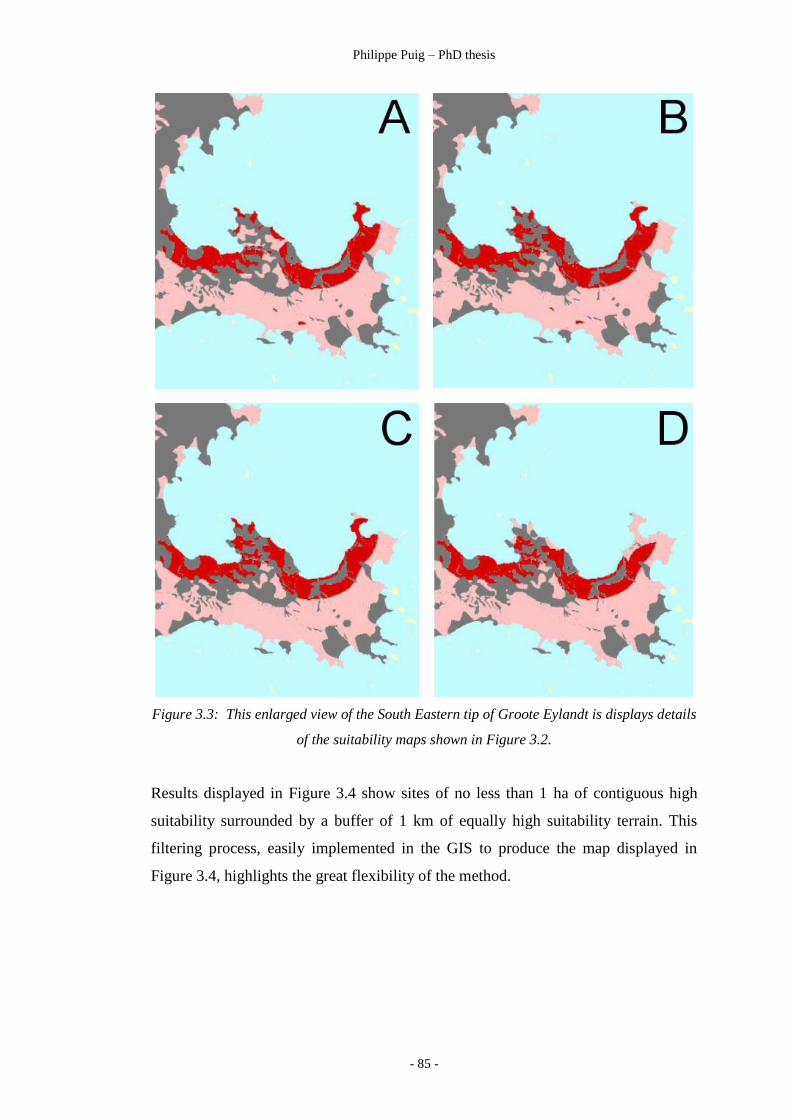
Philippe Puig – PhD thesis
- 85 -
Figure 3.3: This enlarged view of the South Eastern tip of Groote Eylandt is displays details
of the suitability maps shown in Figure 3.2.
Results displayed in Figure 3.4 show sites of no less than 1 ha of contiguous high
suitability surrounded by a buffer of 1 km of equally high suitability terrain. This
filtering process, easily implemented in the GIS to produce the map displayed in
Figure 3.4, highlights the great flexibility of the method.

Philippe Puig – PhD thesis
- 86 -
Figure 3.4: Final map showing location of areas suitable for prawn aquaculture. Core
regions of higher prawn aquaculture suitability in red show areas of no less than 1 ha of
land of highest suitability to prawn farming surrounded by a further 1km buffer of highly
suitable ground.
3.3.3 Validation of the model
Final validation can only be performed by field work. A visual investigation of sites,
however, provides experts with visual clues sufficient to confirm initial indications
of the model. This visual assessment was performed from oblique aerial photography
acquired by the NT Government during a qualitative survey of the North East
coastline of the Northern Territory in 1999. Plate 3.1 below reveals the type of
environment deemed suitable by the model described for the establishment of a
prawn farm. Although an aquaculture expert cannot visually confirm the suitability
of all sites identified by the model from the incomplete aerial photographic coverage
of the Groote Eylandt coast line, photos such as Plate 3.1 reflect, in that location, the
validity of the model output.

Philippe Puig – PhD thesis
- 87 -
Figure 3.5: Oblique aerial photograph of site B2. The site is located east of the entrance of
South Bay on Bickerton Island.
3.4 Discussion
Malczewski (1999: p.130) writes “Here we limit our discussion to the trapezoidal
numbers” although he admits that triangular membership functions fall in the same
category of most often used membership functions. He does not explain why, in the
context of MCDA he prefers them to triangular membership functions. Malczewski
(1999: p. 186) recognises two drawbacks of pair wise comparisons to assign criterion
weightings: questionable meaningfulness and rapidly escalating demand put on
decision makers when the number of criteria exceeds 10. However, Malcewski (1999:
p.187) stresses that, in support of pair wise comparisons for criterion weightings, the
method has been tested for spatial decision making and built into IDRISI GIS
(Eastman, 2009) decision-making module. Although trapezoidal membership
functions and pair wise comparisons are not used elsewhere in this thesis, they stand
as a reminder of the variety of techniques not considered in this thesis as they do not
lead to simpler GIS modelling procedures.
Reiterating caveats in section 3.1, parallels can be drawn between fuzzy multicriteria
decision analysis described by Malczewski (1999) and other similarly non
mainstream spatial applications of fuzzy logic (Burrough et al., 1992, Costa Fonte
and Lodwick, 2005, Lagacherie et al., 1996). All are well suited to a specific domain
of application. Their scope, however, is rather limited. In this instance, Malczewski’s
(1999) spatial fuzzy multi criteria decision analysis was selected because of its broad
range of NRM applications from marine, to mine site rehabilitation and weed control.

Philippe Puig – PhD thesis
- 88 -
Ultimately, AAGIS was well received by the NT Government and other NRM
specialists (Puig, 2005; Puig, 2008).
The implementation of fuzzy logic described in this chapter shares similarities with
the work of Burrough (1998) on fuzzy boundaries. They are sufficiently visually
explicit to be easily understood, unfortunately, their range of applications is rather
limited. They do not link to fuzzy rule-based modelling, unquestionably the most
prolific application of fuzzy logic. The approach adopted was initially prompted by
the need for a methodology able to facilitate the inclusion of Aboriginal knowledge
in the GIS model. Giving the local community a sense of ownership of this land
management tool was another desirable aspect of the solution adopted. Surveys,
similar to that detailed in section 5.3, were to be carried out, in collaboration with
anthropologists and linguists, to capture an oral traditional knowledge reliant on
terms which generally meet the criteria of the “sorites” paradox outlined in section
1.1. Fuzzy logic, widely recognised as best suited to the capture of human knowledge,
a view strongly supported by Chapter 5, was consequently well adapted to the task.
Unfortunately, contrary to the initial scope of the project, the intended capture of
traditional human knowledge, in the context of this survey, turned out to be
impossible for two completely independent reasons. The budget of this project was
limited and did not allow for an anthropologist to spend on Groote Eylandt the time
necessary to speak to traditional experts. In addition, prawns do not appear to have
played an important role in the diet of Aboriginal cultures of the Northern Territory.
Little traditional knowledge of prawns is therefore likely to exist on Groote Eylandt.
Other traditional knowledge may, however, be highly relevant particularly in relation
to seasonal bad weather such as rough seas and storms which may affect coastal
prawn farms. However, owing to a limited budget, no capture of traditional
knowledge of relevant local weather patterns was attempted.
Advantages of this fuzzy suitability analysis are noteworthy. Various ranges of
possible values taken by all environmental variables selected are defined in linguistic
terms. Those are less likely to disenfranchise the broad spectrum of stakeholders
often associated with NRM projects. The model can be described in non technical
terms thus facilitating cross cultural dialogues as the linguistic terms used are readily
translated in any local language. The original output of this model consists of 4 maps

Philippe Puig – PhD thesis
- 89 -
instead of one as would be normally expected. Users are therefore visually reminded
that the conclusion reached by such a model is not absolute. The extreme possible
interpretations of the linguistic terms of suitability impose upper and lower limits on
the final result. In this instance the intermediate interpretation, as well as the upper
and lower limits, are parts of the model output. A corollary of the previous statement
is the need to provide as well the single and easily readable output generally
requested by end users. The approach adopted here directly involves them in
designing their defuzzification procedure. Consequently the model output matches
very closely the user’s needs.
A different choice of membership function could result in an improvement of the
strategy described here. If instead of trapezoidal membership functions
recommended by Malczewski (1999), triangular membership functions defined in
Chapter 2 are selected, the whole procedure remains unchanged and 3 maps A, B and
C instead of 4 are generated. The central map B is then in sharper contrast with the
two extreme maps A and C. Map B could then be the single output of the model.
Maps A and C would represent the limits of the suitability displayed in B.
Advantages of this adaptation of Malczewski’s method include simpler membership
functions and the elimination of the duplication of information in central maps B
and C. Although not a path-breaking improvement, the adoption of triangular
membership functions instead of trapezoidal membership functions is consistent with
the approach to membership functions design adopted throughout this thesis and
removes the plateau of the membership function which carries no information and
plays no role in that context.
The close involvement of aquaculture specialists and other stakeholders in the
modelling process is a key advantage of this strategy. Although only two DAC
experts contributed their knowledge to this project, the methodology is clearly
scalable. Linguistic and anthropological support would make it very well suited to
predictive modelling based on a combination of Aboriginal and Western knowledge.
Although Aboriginal knowledge has been recorded in Northern Australia for more
than 20 years, Smith (2008) deplores a lack of effective implementation in
environmental models where it would matter most.
Summary

Philippe Puig – PhD thesis
- 90 -
The Anindilyakwa Aquaculture GIS relies on fuzzy multicriteria suitability analysis
to identify the best locations for prawn farming on the coast of Groote Eylandt and
Bickerton Island in the remote Gulf of Carpentaria. Raster GIS’s flexibility facilitates
the creation of a model of site suitability comprised of 10 layers of environmental
data. Fuzzy logic, through linguistic terms and their equivalent membership
functions incorporates in the model the knowledge of two aquaculture experts. The
modelling framework described in this chapter enables a number of specialists to
merge their respective expertise. Their knowledge is expressed in two components of
this model: membership functions and weightings. The former are derived from
linguistic terms of suitability of the different ranges of values of the environmental
variables considered. The latter reflect the relative importance of the respective
environmental variables and their associated membership functions. Trapezoidal
membership functions of each of the 10 environmental variables are represented by
their 4 coordinates from which 4 maps are derived for each variable. Once merged,
the matching maps of the 10 variables scan the range of possible interpretations of
the different levels of suitability of the coastline for prawn farming. Although the
method described relies on trapezoidal membership functions, triangular membership
functions may be preferable as they would eliminate some duplication of visual
information.
The final product is a single map of suitability for prawn farming that summarises all
aquaculture expertise and environmental data available at the time. This map of
suitability for aquaculture prawn farming is defuzzified, to meet the end user’s wish,
by merging all available information to extract the 5 most suitable areas. The aerial
photography of one of the five areas identified by this desktop GIS analysis confirms
its suitability to prawn farming.
This case study highlights two advantages of this approach to site suitability analysis.
The highly visual nature of the solution, to be expected from a GIS analysis, greatly
facilitates communications between the modeling team and all stakeholders. The
process of inclusion of experts’ knowledge is well suited to the development of a
decision making tool easily adaptable to a wide range of technical requirements and

Philippe Puig – PhD thesis
- 91 -
cultural backgrounds. DAC experts found the process of weightings evaluation by
pair wise comparison challenging. Although both highly qualified in their domain,
one systematically assigned more importance to economical considerations while the
other was driven by environmental concerns. In the end their complementary views
were all merged in the model. Nowhere else in this thesis is fuzzy logic so integrated
within a GIS modelling methodology. Fuzzy logic, however, does not modify any
fundamental GIS functionality. Instead, fuzzy logic considerably enhances the
information content of the graphical solution displayed in the final map. Figure 3.4
captures the consensus reached by two experts despite somewhat diverging views on
site suitability. Figure 3.4 does not suggest where to carry out field surveys on the
basis of a blunt Boolean classification of the natural environment. Instead, our innate
tendency to incorporate moderated beliefs in our decision making process is
implemented in a series of 4 maps representing the range of possible interpretations
of all grades of suitability considered. The final map of suitability is therefore an
information rich document well adapted to different levels of use calling for different
depths of interpretation. A parallel can be drawn with the role played by statistics in
GIS modeling. Beyond the graphical output of the GIS, statistics allow one to
question the reliability of the solutions emerging from a map. The number of samples
and their distributions in the different regions of the model will help users to develop
a better understanding of the underlying reliability of the visual output of the GIS.
The case study explored in this chapter aims at producing an information enriched
GIS model. Statistics do so by incorporating in the model an in depth understanding
of the variability of the data. Fuzzy logic, in the context of this chapter, strives to
emulate humans’ natural ability to constantly generate simple models, based on
readily available information, to make sense of their surrounding. This case study is
an example of the synergy resulting from the combined use of GIS and fuzzy logic to
improve the management of natural resources. The product is an information rich yet
simple map of site suitability.

CHAPTER 4
DATA DRIVEN FUZZY RULE-BASED MODELLING

Philippe Puig – PhD thesis
- 93 -
Overview
This chapter focuses on objective fuzzy rule-based modelling. In this chapter,
principles introduced in Chapter 2 are applied to three practical examples of data
driven modelling. They illustrate how fuzzy rule-based modelling addresses two
common tasks of GIS modelling: classification and prediction. Small datasets of high
dimensionality, in the case studies considered, are of particular relevance to GIS
modelling. The simple fuzzy rule-based approach to predictions from high
dimensionality datasets, proposed in this thesis, is first tested on a popular dataset
then evaluated against a more sophisticated fuzzy rule-based method. A complex
multivariate NRM case study finally provides an opportunity to compare the same
fuzzy rule-based modelling strategy with statistical techniques adopted in advanced
ecological modelling.
.
Principles of fuzzy rule-based classification are introduced in a case study based on
Fisher‟s iris dataset downloaded from the Monash University web site
(http://www.csse.monash.edu.au/~lloyd/tildeFP/). In this dataset, containing 150
records, each iris flower, described by the length and width of its petals and sepals,
belongs to one of three varieties. A fuzzy rule-based model is derived from this
dataset. Its performance with weighted and non weighted rules is evaluated.
Fuzzy rule-based predictions from high dimensionality datasets are demonstrated on
two case studies. The first case study, based on Nakanishi‟s paper (Nakanishi et al.,
1993) describes a sophisticated technique for the objective identification of fuzzy
rule-based models. A simplified method is applied to data provided by Nakanishi
(Nakanishi et al., 1993, p. 279). The dataset comprises 70 records of five input and
one output variables from the operation of a chemical plant. The simplified method
proposed is compared with Nakanishi‟s. In the second case study, the simplified
fuzzy rule-based modelling strategy previously tested is used to revisit a study of the
influence of environmental variables on foraging patterns of elephant seals. The
small dataset of 50 records and 14 variables is well suited to a demonstration of the
contribution of fuzzy rule-based modelling to NRM studies where advanced
statistical techniques, such as GAM and GLM in this case, often prevail.

Philippe Puig – PhD thesis
- 94 -
4.1 Application of fuzzy rule-based modelling to classification
Fisher‟s iris dataset (Fisher, 1936) lists widths and lengths of petals and sepals of
varieties of iris flowers. Fifty records of petal and sepal widths and lengths are listed
for each of the three following varieties: setosa, virginica or versicolor. Fisher used
this dataset to teach his students multivariate analysis. Popular in pattern recognition
and artificial intelligence circles to test algorithms performance, these data are well
suited to demonstrate how to build a fuzzy rule-based model. The data can be
obtained from websites listed in Appendix 3. A number of similar versions of this
dataset exist. They differ in their spelling of iris varieties and in the units used to
measure the lengths and widths of petals and sepals. The dataset used here was
downloaded from the Monash University website. The dataset is reproduced in
Appendix 4.
The model described below is predictive in the sense that it predicts the iris variety
from measurements of length and width of petals and sepals of a flower. At the same
time it can be considered as an example of fuzzy classification (Chen and Fang, 2005;
Chiu, 1997). Fuzzy rule-based modelling can clearly serve a variety of purposes.
However, instead of focusing on the purpose of the model, this chapter demonstrates
how fuzzy models cope with different type of data. In this case study the output is
categorical (variety of flower) and inputs are continuous ratio variables
(measurements of length and width). A randomly selected sample of 10 out of a total
of 150 records is displayed below.
Table 4.1: Subset of Fisher’s iris dataset. The 3 varieties of iris flowers setosa, versicolor
and virginica are identified on the basis of flower metrics: petal and sepal width and length.
The approximation of a linear function in section 2.6.1 is a relatively simple
univariate problem. Many readily available data fitting algorithms could be used

Philippe Puig – PhD thesis
- 95 -
instead of a fuzzy rule-based model to provide good predictions of y from values of x.
The iris dataset belongs to the multivariate category which typically requires more
sophisticated approaches. The model described below relies on the same strategy
described in section 2.6. This generic, scaleable, approach to quantitative as well as
qualitative predictions is one of the advantages of fuzzy-rule based models. To create
a fuzzy rule-based model capable of predicting the flower variety from flower
metrics listed in this table, we must first identify all input and output membership
functions, as well as the rules they define, along with their weightings if necessary.
4.1.1 Identification of the parameters of a fuzzy rule-based model
This phase of development of the model is generally referred to as “identification”.
Plotting all input variables, one by one, against the output variable often reveals
interesting properties of a dataset.
Figure 4.1: Plots of iris varieties versus flower metrics. Setosa, versicolor and virginica
varieties correspond to codes 1, 2 and 3 respectively.
Figure 4.1 shows that out of the 4 flower metrics considered, sepal length is the least
representative of a single iris variety. Sepal length shows a substantial overlap of the
three classes and should therefore have lower weightings. The first step in fuzzy rule-
Philippe Puig – PhD thesis
- 96 -
based modelling consists of translating the initial dataset into membership functions.
Two dimensional fuzzy patches are used in the first model explored as both variables
are numerically continuous. Categorical outputs in this model are coded below. This
code was selected for its simplicity. Any three equal consecutive intervals are
suitable. Corresponding code numbers assigned to the three categories are then the
centre of the corresponding interval. Encoding these categories with non contiguous
numbers could result, for instance, in flowers not being assigned to any existing class
rather than being misclassified.
setosa range [0,1] class code = 1
versicolor range [1,2] class code = 2
virginica range [2,3] class code = 3
Fuzzy patches are one-dimensional in this model. Measurements of length and
widths of petals and sepals in Figure 4.1 and 4.2 are plotted in the middle of the
corresponding output range. The model associates setosa with all output values
between 0 and 1, versicolor with all values between 1 and 2 and virginica with values
between 2 and 3. For practical purpose all categorical output values of the training
dataset are assigned to the middle of their corresponding range: 0.5 for setosa, 1.5 for
versicolor and 2.5 for virginica. A subset of 120 randomly selected flowers is
extracted from the original dataset to train the model. The remaining 30 records will
be used to assess its performance. Figure 4.2 and 4.3 as well as Table 4.2, 4.3 and 4.4
refer to this randomly selected subset, not to the complete dataset. As the sample is
randomly selected we have a slightly different number of records of each iris variety:
40 setosa, 37 vertosa, 43 virginica. Membership functions can now be derived from
the experimental dataset.
Many flowers have identical measurements and consequently a number of records
are plotted in the same location in Figure 4.1. A flower cannot belong to two
different varieties at once: the vertical axis is consequently Boolean. Two flowers of
different varieties may have the same petal or sepal width or length: the horizontal
axis is therefore fuzzy. The resulting fuzzy patches only have one fuzzy dimension
(on the horizontal axis) and are no longer represented by rectangles but by lines

Philippe Puig – PhD thesis
- 97 -
(Figures 4.2 and 4.3). Fuzzy membership functions, drawn on the vertical axis,
would have no height. They are flattened rectangles corresponding to the orange,
blue and red thick lines on the vertical axis. They are trapezoidal membership
functions with no overlap defined below by their trapezoidal fuzzy number.
setosa (0,0,1,1)
versicolor (1,1,2,2)
virginica (2,2,3,3)
Figure 4.2: Membership functions of petal length and petal width. Iris variety setosa,
versicolor and virginica are plotted on the horizontal axis in orange, blue and red,
respectively. Y values are the centre of the range of the corresponding flower class. X values
are measurement in cm of the metric displayed. Circles with a cross are centroids of metric
measurements: they define the apex of the respective membership functions.
Here we have a practical design for fuzzy rule-based models predicting categories
from fuzzy input variables. In the training dataset all output will be coded as 0.5 for
setosa, 1.5 for versicolor, 2.5 virginica: that is the centre of the range of possible
values for the corresponding Iris variety. Figure 4.2 and 4.3 allow us to make a
number of observations. Owing to different amount of overlap between membership

Philippe Puig – PhD thesis
- 98 -
functions, the twelve membership functions and therefore the twelve corresponding
rules of the resulting predictive model do not have the same discriminating power.
Petals will be more useful to identify species than sepals as sepal membership
functions overlap a lot more. Iris setosa is uniquely identified by small petals, smaller
than both versicolor and virginica. The least useful variable is sepal width as the
three membership functions overlap so much that only some iris setosa (light grey
triangle in the lower panel of Figure 4.2) have sepals distinctively wide. Sepal widths
are particularly unreliable as all versicolor sepal widths could be identified as setosa
or virginica instead. Petal length is best at separating the three varieties as the
percentage overlap between successive membership functions is lowest.
Figure 4.3: Membership functions of sepal length and sepal width.
The previous qualitative description of the role the different variables play in the
model is important. It provides a clear understanding of what drives the classification
of these three species without having to rely on mathematical expressions, whose
significance is rarely equally understood by all members of a multidisciplinary
research team. Comments above need to be reflected in the model. Independent
variables poorly related to the dependent variable have a low correlation coefficient.

Philippe Puig – PhD thesis
- 99 -
The assumption is of course that the type of relationship between the two variables is
known. This relationship is generally considered to be linear. If the relationship is not
linear it should be made linear by applying a suitable expression to the data. This is
not always feasible and, consequently, weightings are often ignored in this thesis
particularly when dealing with small noisy datasets. Here however they are
calculated to demonstrate that they can be effective with some datasets.
The more records in a membership function the more representative and reliable its
contribution to the final model. The density of records is the metric used here to
capture this property. More membership function metrics could be explored to
calculate weightings. However, simplifying calculations is one of the most important
objectives of fuzzy rule-based modelling. One has therefore to restrain from
introducing a level of sophistication which would contradict the initial intent of this
dissertation.
Table 4.2: Minimum, maximum, number of values (N Points), density, correlation coefficient,
weighting and normalized weighting of the 4 flower metrics for the 3 iris varieties.
All information relevant to a fuzzy rule-based model that can be derived from
Figures 4.2 and 4.3 is captured in Table 4.2. Density is the number of values divided
by the range of values in the membership function. This corresponds to the number
of points divided by the difference between the maximum and minimum. The
correlation coefficient is directly derived from the input data. Weightings are the
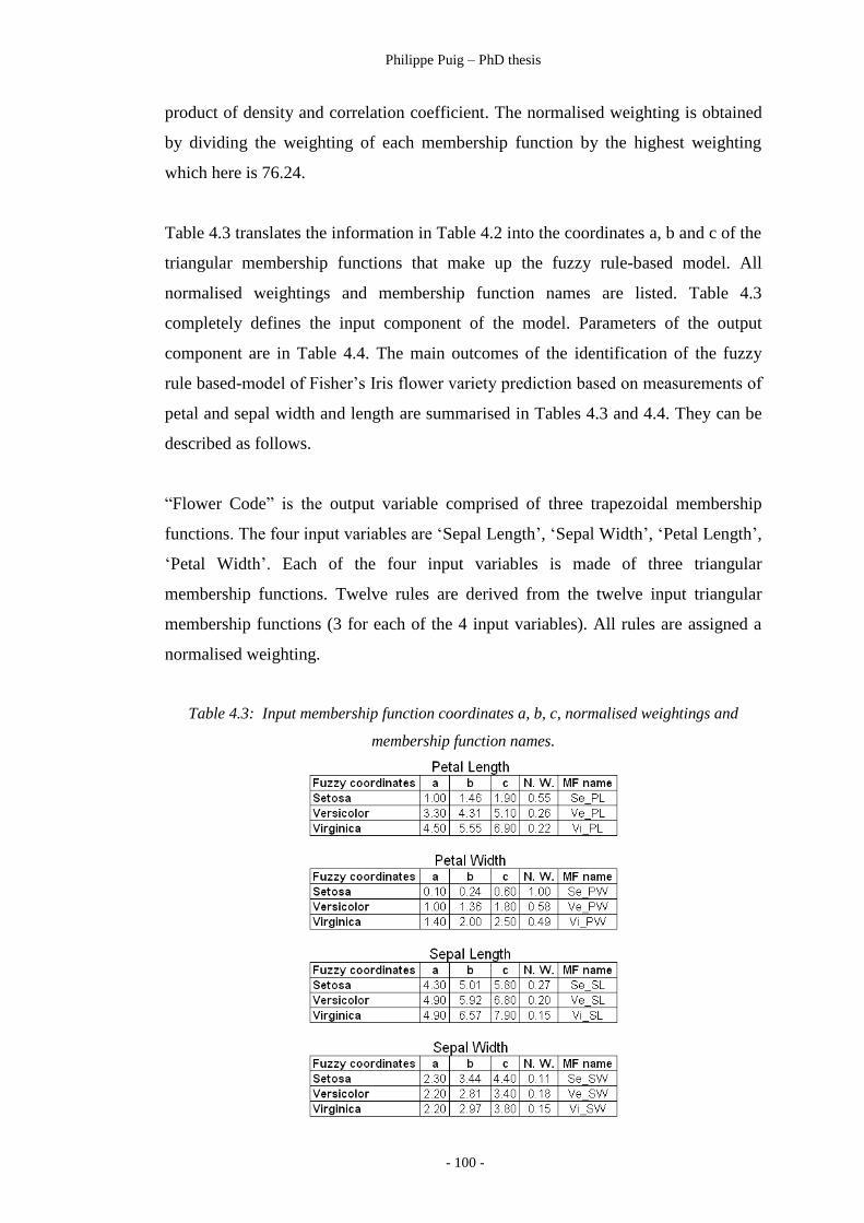
Philippe Puig – PhD thesis
- 100 -
product of density and correlation coefficient. The normalised weighting is obtained
by dividing the weighting of each membership function by the highest weighting
which here is 76.24.
Table 4.3 translates the information in Table 4.2 into the coordinates a, b and c of the
triangular membership functions that make up the fuzzy rule-based model. All
normalised weightings and membership function names are listed. Table 4.3
completely defines the input component of the model. Parameters of the output
component are in Table 4.4. The main outcomes of the identification of the fuzzy
rule based-model of Fisher‟s Iris flower variety prediction based on measurements of
petal and sepal width and length are summarised in Tables 4.3 and 4.4. They can be
described as follows.
“Flower Code” is the output variable comprised of three trapezoidal membership
functions. The four input variables are „Sepal Length‟, „Sepal Width‟, „Petal Length‟,
„Petal Width‟. Each of the four input variables is made of three triangular
membership functions. Twelve rules are derived from the twelve input triangular
membership functions (3 for each of the 4 input variables). All rules are assigned a
normalised weighting.
Table 4.3: Input membership function coordinates a, b, c, normalised weightings and
membership function names.

Philippe Puig – PhD thesis
- 101 -
Output memberships are defined as the three non overlapping trapezoidal
membership functions in Table 4.4. They are typical of rule-based models with fuzzy
input and Boolean output.
Table 4.4: Coordinates of the 3 non overlapping trapezoidal output membership functions
corresponding to the 3 iris varieties setosa, versicolor and virginica.
Previous observations of the relative lack of relevance of the flower metric sepal
width are confirmed by its very low weightings in Table 4.3. This flower metric is
therefore discarded as Figure 4.3 shows a near complete overlap of all 3 membership
functions for this metric. The final model comprises therefore 9 rules. From Table
4.3 and 4.4 we can write:
Rule 1 IF Input MF is Se_PL THEN Output MF is Setosa NW= 0.55
Rule 2 IF Input MF is Ve_PL THEN Output MF is Versicolor NW= 0.26
Rule 3 IF Input MF is Vi_PL THEN Output MF is Virginica NW= 0.22
Rule 4 IF Input MF is Se_PW THEN Output MF is Setosa NW= 1.00
Rule 5 IF Input MF is Ve_PW THEN Output MF is Versicolor NW= 0.58
Rule 6 IF Input MF is Vi_PW THEN Output MF is Virginica NW= 0.49
Rule 7 IF Input MF is Se_SL THEN Output MF is Setosa NW= 0.27
Rule 8 IF Input MF is Ve_SL THEN Output MF is Versicolor NW= 0.20
Rule 9 IF Input MF is Vi_SL THEN Output MF is Virginica NW= 0.15
All rules in this case study have single conditions. Indeed multiple conditions
concatenated by AND, OR, XOR, NOT operators described in section 2.7.4 can
replace single conditions. However, complex conditional combinations, frequent in
control systems, are less common in fuzzy rule-based models of natural systems. The
complexity of actual interactions between input and output variables in natural
systems is better described by multiple simple rules linking a single antecedent to a
single consequence. This view is reinforced by the two fuzzy rule-based models
presented in Chapter 5.

Philippe Puig – PhD thesis
- 102 -
4.1.2 Building the fuzzy rule-based model
The fuzzy rule-based model is implemented in Matlab (MathWorks, 1999) with
weightings, and in Scilab (Campbell et al., 2006) without weightings. The Scilab
fuzzy logic toolbox (Urzua, 2004), in version 0.2 used here, does not implement
weightings.
Figure 4.4: Screenshot of the Matlab Fuzzy Logic Toolbox (FLT). FLT provides a clear
diagrammatic description of the structure of a fuzzy rule-based model.
Once all the parameters of the model defined during the identification phase
completed in section 4.1.1 are entered, the model can be run to classify iris flowers
from the length and width of petals and length of sepals. The parameters selected for
the Matlab model are displayed in Figure 4.4. The Matlab rule viewer in Figure 4.5
shows how each variable (yellow) contributes, through sepal and petal measurements
displayed in the Input window, to the iris flower classification. The process leading
to the calculation of the output by centroid defuzzification is easy to follow. The
Matlab graphical representation of the contribution (blue) of each rule to the
classification output helps to develop a clear understanding of the model.

Philippe Puig – PhD thesis
- 103 -
Figure 4.5: Screenshot of the Matlab Fuzzy Logic Toolbox (FLT) rule definition window.
4.1.3 Assessing the fuzzy model performance
The performance of the models with and without weightings is assessed on the
ability to correctly classify 30 flowers defined by the three first rows of flower
metrics displayed in Table 4.5. These 30 records are not part of the 120 records used
to train the model in Chapter 4.1.1. We are therefore assessing the ability of the
model to correctly process unknown information.
Table 4.5 shows that the weighted classifier made only one error out of thirty
predictions while the non weighted classifier failed to correctly classify four flowers.
The weighted classifier performs best. The comparison between the predictions of
the two models, however, shows that in only one instance their predictions are
substantially different. The 0.96 correlation coefficient between outputs of the
weighted and non weighted models displayed in Figure 4.6 confirms that their

Philippe Puig – PhD thesis
- 104 -
predictions are very similar. However, the classification based on weighted rules, as
displayed in Table 4.5, performs better.
Table 4.5: Performance of the model with and without weightings. Predicted values in red
indicate misclassified flowers. The classification with weightings performs best with an
accuracy of 29/30 = 96.67%.
The iris dataset in this case study, initially used by Fisher (1936) to demonstrate the
principles of discriminant analysis (Kachigan, 1991), has become a standard test data
set for a wide range of classification methods (Chiu, 1997; Halgamuge, 1997;
Ishibuchi and Nakashima, 2000; Kumar and Sirohi, 2010; Lee et al., 2006; Lee; 2009;
Ling, 2009; Nakashima et al., 2002; Qiu et al., 2007). Chen and Fang (2005: p. 47)
show that the 6 fuzzy rule-based methods they compare, on Fisher‟s (1936) dataset,
achieve classification accuracies between 94.67% and 96.67% while their own
improved method reaches 97.33% . Lee (2009: p. 85) lists six additional fuzzy based
methods, tested on the same dataset with similar classification accuracies between
96.00% and 97.12%. Table 4.5 shows that the method proposed in this thesis,
particularly with weighted rules, has a classification accuracy of 96.67% on par with
other method based on fuzzy logic.
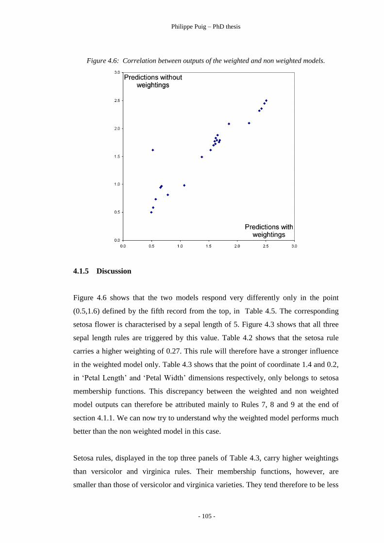
Philippe Puig – PhD thesis
- 105 -
Figure 4.6: Correlation between outputs of the weighted and non weighted models.
4.1.5 Discussion
Figure 4.6 shows that the two models respond very differently only in the point
(0.5,1.6) defined by the fifth record from the top, in Table 4.5. The corresponding
setosa flower is characterised by a sepal length of 5. Figure 4.3 shows that all three
sepal length rules are triggered by this value. Table 4.2 shows that the setosa rule
carries a higher weighting of 0.27. This rule will therefore have a stronger influence
in the weighted model only. Table 4.3 shows that the point of coordinate 1.4 and 0.2,
in „Petal Length‟ and „Petal Width‟ dimensions respectively, only belongs to setosa
membership functions. This discrepancy between the weighted and non weighted
model outputs can therefore be attributed mainly to Rules 7, 8 and 9 at the end of
section 4.1.1. We can now try to understand why the weighted model performs much
better than the non weighted model in this case.
Setosa rules, displayed in the top three panels of Table 4.3, carry higher weightings
than versicolor and virginica rules. Their membership functions, however, are
smaller than those of versicolor and virginica varieties. They tend therefore to be less

Philippe Puig – PhD thesis
- 106 -
influential during the COG defuzzification as bigger membership functions pull the
centroid more towards them. For the same membership value, during the aggregation
process, the answer will be more strongly influenced by the bigger membership
functions. Only weightings can counteract this effect which is particularly relevant in
that case as „Sepal Length‟ triggers all three membership functions at once. Two
larger non setosa membership functions influence the answer. Their effect can only
be countered effectively by weightings.
In all 3 remaining cases of flowers misclassified by the non weighted model, the
discrepancy between the outputs of both models is generally small. This observation
supports a general impression conveyed by this thesis, and reinforced in Chapter 5,
that Mamdani type fuzzy rule-based models with ratio valued inputs and output
rarely benefit much from weightings. In the case of models with a categorical output,
a small variation in output can result in a different category and consequently a very
serious error. In that case weighted rules may be advantageous when the COG
defuzzification is used.
4.2 Multivariate predictive modelling on the basis of variables of
unknown influence on the outcome
Generalised linear models (GLM) have grown in popularity among ecologists during
the last three decades (Guisan et al., 2002). The sophistication and capabilities of
advanced statistical modelling tools are not without impediments. Experiments often
need to be carefully designed to meet underlying requirements (Stern et al., 2004).
These conditions are rarely met by NRM datasets. Within this context additional
effort and expertise are not justified as they are unlikely to translate into substantially
better predictions. The reason is simple: predictive capability is limited by the nature
and quality of the data. This chapter proposes a less onerous methodology well suited
to NRM datasets.
Section 4.2.1 introduces a generic semi automatic data driven fuzzy rule-based
modelling methodology to tackle multivariate predictive models where both input
and output variables are numerical. Section 4.2.2 applies this modelling strategy to

Philippe Puig – PhD thesis
- 107 -
real experimental data on elephant seal wanderings in the Southern Ocean.
Predictions of foraging patterns of elephant seals obtained by this method are
compared with GLM results (Bradshaw et al., 2004).
4.2.1 A generic semi automatic data driven fuzzy rule-based methodology to
tackle multivariate predictive models
This case study has three objectives. Firstly, Nakanishi et al.‟s strategy (1993) of
semi automatic data driven fuzzy rule-based modeling is presented. Secondly, a
simplified approach to Nakanishi‟s strategy is proposed. Thirdly, the performance of
the two methods is compared.
4.2.1.1 Nakanishi‟s identification method
Nakanishi et al. (1993) offer an elegant and practical identification method
summarised in 8 steps:
1/ split the initial dataset in 2 subsets containing an equal number of records:
one is used to train the model, the other to assess it;
2/ split in two the training subset: these two subsets are used to identify initial
variables to retain in the model;
3/ a fuzzy clustering algorithm is used to segment the training datasets;
4/ one model is created from each of the two training subsets with fuzzy
membership values generated by fuzzy clustering;
5/ each of these two models is evaluated with data generated from the other
model;
6/ predictions from both models are evaluated as all rules are progressively
incorporated, one variable at a time;
7/ variables that produce incompatible predictions are eliminated;
8/ the model comprised of the remaining variables is assessed on the evaluation
dataset.
Nakanishi et al.‟s (1993) article is particularly useful as it provides a practical
technique to design membership functions and a sensible method to pick variables to
include in the model. This 8 step strategy, however, is involved and time consuming
and tends to defeat the purpose of fuzzy logic.

Philippe Puig – PhD thesis
- 108 -
In steps 1 to 3 Nakanishi et al.‟s (1993) method produces trapezoidal membership
functions that often provide a better representation of reality than triangular
membership functions as they allow more than one value to perfectly represent a
class. The equations of the two sloping sides are provided by the regression lines that
interpolate, on each side, all experimental membership values between 0 and 1. The
intersection of these two lines with (x) = 0 and (x) = 1 provides the four vertices
of the trapezoidal membership function. The membership function (x) represents
the membership of a record to a class created by fuzzy clustering in Step 3.
Calculating the equation of the regression line can be avoided by identifying visually,
from a plot of records versus their membership value, which records should be the
vertices of each membership function. The visual approach is advantageous as it does
not require writing a script that will decide which points to regress. This decision is
difficult to embed in an algorithm as the leftmost and rightmost records of each
membership function do not necessarily correspond to records with a null
membership.
In steps 4 to 8 Nakanishi et al. (1993) propose a very elegant solution to the problem
of deciding which variables to include in the model. They do not rely on any
statistical method to choose variables that are good predictors of the output. The role
of non statistical models is important where two fundamental statistical premises are
ignored: independence of data and undefined distribution. Independence of data
rarely occurs when dealing with georeferenced field records, a common problem in
NRM surveys. In this context field records are frequently either auto correlated or
spatially correlated. Both instances contravene the assumption of independence of
data. The statistical distribution of NRM data is often unknown. This is inherent to
the nature of fieldwork. For reasons of prohibitive cost of acquisition and practicality,
datasets are often too small (less than 50 records) to allow field records to be
meaningfully fitted to any statistical law of distribution. Geostatistics address the
issue of spatial correlation, however a major intrinsic limitation (Houlding, 1999)
remains. Records need to be normally distributed. As mentioned previously this
condition is often difficult to meet as the dataset cannot be normalised if the initial
distribution cannot be unambiguously identified because the dataset is too small. The
simplified fuzzy rule-based modelling method described in the next section ignores
statistical tests to provide GIS modellers stand-alone investigative tools.

Philippe Puig – PhD thesis
- 109 -
4.2.1.2 A rationale for simplifying Nakanishi et al.‟s (1993) fuzzy rule-based
modelling strategy
Nakanishi et al.‟s (1993) approach to fuzzy rule-based modelling is very
comprehensive but time consuming. It provides the material required to demonstrate
the simplified fuzzy rule-based modelling strategy advocated in this thesis. GIS
specialists are often requested to predict properties across a landscape. They have to
rapidly ascertain the predictive capability of available multivariate datasets. The first
step generally consists in checking the correlation coefficient between the output and
all potential input variables. Although very low correlation coefficients immediately
identify input variables that can be discarded, those with intermediate correlation
coefficients are more difficult to handle. A fundamental question thus remains: does
the dataset allow the prediction of values of output variables? The strategy proposed
intends to unambiguously answer this question in the most efficient manner.
Let us first review Nakanishi‟s eight step approach to only retain steps which are
crucial to assess the predictive capability of the dataset. The intention is not to
dismiss Nakanishi et al.‟s (1993) excellent method but to simplify it in order to
provide a faster first pass approach capable of suggesting whether or not the
predictive capability of the dataset warrants the additional time and effort required by
Nakanishi et al.‟s (1993) technique. Steps 1 and 2 are eliminated as the whole dataset
is often required to estimate its predictive capability. Step 3 is retained because a
fuzzy clustering algorithm will rapidly process a vast volume of data with minimum
human intervention. Steps 4, 5 and 6 are eliminated because the priority is to make
sure that predictions are possible, not to refine the model. Step 7 is retained as
variables without predictive power need to be eliminated as soon as possible. Finally,
step 8 is retained. Compared with Nakanishi‟s method, the predictive capability
estimated will be optimistic because it relies on the same dataset for the identification
and evaluation of the model. If the correlation coefficients between predicted and
observed outputs are low we can therefore be sure that no predictive model can be
created.
The simplified fuzzy rule-based modelling strategy proposed is a three step process.
Firstly, a fuzzy clustering algorithm derives all identification parameters from the

Philippe Puig – PhD thesis
- 110 -
whole dataset. Secondly all variables that produce unacceptably erratic membership
functions are eliminated. Thirdly, the model created from the remaining variables is
evaluated on the whole dataset. If it can be established that a predictive model is
feasible, additional time may be allocated to refine the predictions. A GLM or other
sophisticated statistical model may then be preferred. If the prediction capability of
the model is poor there is little chance that additional effort will result in
substantially better predictions. The relevance of the dataset to the problem
investigated needs to be reconsidered before additional resources are committed to
modelling.
4.2.1.3 Simplified semi automatic segmentation of Nakanishi‟s dataset
One of three datasets in Nakanishi et al.‟s (1993, p.279-280) paper is reproduced in
Table 4.6 below. Table 4.6 contains seventy records of five input and one output
variables defining a process in a chemical plant. These variables are listed below.
X1 = monomer concentration
X2 = change of monomer concentration
X3 = monomer flow rate
X4 = local temperature 1 inside the plant
X5 = local temperature 2 inside the plant
Y = set point for monomer flow rate
To implement the first step of the simplified strategy outlined in the previous section,
all 3 subsets in Table 4.6 are merged into a single dataset. This dataset is segmented
with Fuzme (Minasny and McBratney, 2002) which is a freely available clustering
software created at the University of Sydney. Fuzme performs a semi automatic
segmentation as a good deal of human intervention is required. By comparison,
however, the manual segmentation performed in section 2.1 and leading to the
identification of membership functions in Table 2.2 is subjective. It relies more on
the skills of the modeler.

Philippe Puig – PhD thesis
- 111 -
Table 4.6: Nakanishi’s dataset. The five input and one output variables define a process in a
chemical plant. X1, X2, X3, X4 and X5 are input variables monomer concentration, change
of monomer concentration, monomer flow rate, local temperature 1 inside plant and local
temperature inside plant 2, respectively. Y is the output variable set point for monomer flow
rate.
ID X1 X2 X3 X4 X5 Y ID X1 X2 X3 X4 X5 Y
1 6.59 -0.21 464.00 -0.10 0.10 700.00 18 6.50 -0.09 797.00 0.10 0.10 700.00
2 6.59 0.00 703.00 -0.10 0.10 900.00 19 6.45 -0.09 784.00 0.00 0.10 800.00
3 5.51 -0.29 1782.00 -0.10 0.00 1900.00 20 6.02 -0.18 1211.00 0.00 0.10 1400.00
4 5.62 0.11 3562.00 -0.40 0.10 3700.00 21 5.44 0.01 2404.00 -0.10 -0.10 2500.00
5 5.79 -0.03 3895.00 0.20 -0.10 3900.00 22 5.94 0.17 3701.00 -0.20 0.10 3800.00
6 5.65 -0.14 3887.00 -0.10 0.00 3900.00 23 5.99 -0.03 3896.00 0.20 -0.10 3900.00
7 4.81 -0.23 4462.00 0.00 -0.10 4900.00 24 5.24 -0.24 4048.00 0.10 0.00 4400.00
8 4.72 0.01 5668.00 0.00 -0.10 6000.00 25 4.61 -0.01 5284.00 -0.10 0.20 5400.00
9 4.70 0.05 6368.00 -0.10 0.00 6400.00 26 4.58 -0.14 5844.00 -0.20 0.10 6100.00
10 4.59 0.04 6250.00 -0.20 -0.10 6400.00 27 4.84 0.03 6412.00 -0.10 -0.10 6400.00
11 4.77 0.00 6569.00 0.00 -0.10 6600.00 28 4.77 0.01 6587.00 -0.10 0.10 6600.00
12 4.77 0.03 6779.00 0.00 -0.10 6800.00 29 4.77 0.00 6559.00 0.00 0.00 6700.00
13 4.57 -0.04 6832.00 0.00 0.10 6800.00 30 4.73 0.00 6844.00 -0.10 0.00 6800.00
14 4.56 -0.01 6832.00 -0.10 0.10 6900.00 31 4.71 -0.06 6783.00 0.00 0.00 6800.00
15 4.56 0.00 7022.00 0.00 0.00 7000.00 32 4.48 -0.02 7032.00 0.00 0.00 7000.00
16 4.51 -0.03 6958.00 0.10 -0.10 7000.00 33 4.48 0.00 6973.00 0.00 0.00 7000.00
17 4.50 0.02 7006.00 0.00 0.10 7000.00 34 4.56 -0.01 7009.00 -0.10 0.10 7000.00
35 4.47 0.00 6986.00 -0.10 0.10 7000.00
ID X1 X2 X3 X4 X5 Y
36 6.80 -0.05 401.00 -0.20 -0.10 500.00
37 6.48 -0.02 717.00 -0.10 0.10 700.00
38 6.45 0.00 794.00 -0.20 0.10 800.00
39 6.54 0.06 706.00 -0.20 0.10 800.00
40 6.20 -0.25 792.00 0.00 0.00 1000.00
41 5.80 -0.22 1557.00 -0.20 0.00 1600.00
42 5.43 -0.08 2206.00 -0.10 0.10 2300.00
43 5.51 0.07 2685.00 0.10 0.00 2800.00
44 5.97 0.03 3775.00 -0.10 0.00 3800.00
45 5.77 0.15 3629.00 -0.10 0.00 3800.00
46 6.02 0.05 3829.00 -0.10 -0.10 3900.00
47 5.82 -0.17 3920.00 0.20 -0.10 3900.00
48 5.48 -1.70 3930.00 0.20 0.00 4000.00
49 5.04 -0.20 4448.00 0.00 0.00 4700.00
50 4.62 -0.19 5078.00 -0.30 0.30 5200.00
51 4.54 -0.07 5225.00 -0.30 0.10 5600.00
52 4.71 0.17 5391.00 -0.10 0.00 6000.00
53 4.55 -0.03 6068.00 -0.20 0.00 6400.00
54 4.65 0.06 6358.00 -0.10 -0.10 6400.00
55 4.81 0.11 6379.00 -0.30 0.00 6400.00
56 4.83 -0.01 6416.00 0.10 -0.10 6500.00
57 4.76 -0.07 6514.00 0.00 0.00 6600.00
58 4.73 -0.04 6672.00 0.00 0.00 6700.00
59 4.74 0.01 6775.00 -0.20 0.00 6800.00
60 4.63 -0.07 6849.00 0.00 0.00 6800.00
61 4.66 -0.05 6816.00 0.00 0.00 6800.00
62 4.61 -0.02 6803.00 0.00 0.00 6800.00
63 4.70 0.04 6812.00 0.00 0.00 6800.00
64 4.57 0.01 6998.00 -0.10 0.00 7000.00
65 4.50 0.00 7027.00 0.00 0.00 7000.00
66 4.54 -0.02 6862.00 -0.10 -0.10 7000.00
67 4.54 0.06 6995.00 0.00 0.00 7000.00
68 4.57 0.03 6986.00 0.10 -0.10 7000.00
69 4.48 0.01 6975.00 0.00 0.00 7000.00
70 4.47 -0.04 6998.00 0.00 0.10 7000.00

Philippe Puig – PhD thesis
- 112 -
Much research went into data driven fuzzy rule-based modelling by semi automatic
clustering in the 1980s and 1990s. In depth comparisons (Babuska, 1996) of
clustering algorithms are available in Chapter 2. The Gustafson Kessel algorithm
(Babuska, 1996, p.63) derived from the fuzzy c-means clustering algorithm, can
detect clusters of different shapes and orientation in n dimensional space where n is
the number of variables considered in the model. Fuzme supports the Gustafson
Kessel algorithm used to segment the dataset in Table 4.6. For practical reasons, such
as number of rules and easy assignment of linguistic labels to membership functions,
the maximum number of classes is generally set to nine.
Table 4.7:Effect of the number of clusters on class size disparity. The number of classes in
the first column shows that as the number of classes increases the ratio of the maximum to
minimum number of records per class a to l increases from 2 to5.
Class a b c d e f g h I
2 43 27
3 14 15 41
4 8 13 36 13
5 6 13 26 12 13
6 12 3 3 9 36 7
7 9 11 13 3 26 3 5
8 5 3 14 15 11 10 9 3
9 10 3 10 3 10 11 15 3 5
The more classes, the better the chance to capture in each class one single facet of the
process reflected by the dataset. Modelling one single aspect of a process is easier
and therefore more reliable. However, classes that contain a small number of
elements are likely to be less reliable as they may not contain enough values for a
trend to emerge from the background noise.
Figure 4.7: Effect of minimum number of records per class (N) on number of classes (C).
The influence of a few unreliable records on class parameters may be unacceptable.
There is consequently a balance to maintain between the number of clusters
Philippe Puig – PhD thesis
- 113 -
generated and the number of elements per cluster. Performance indices are calculated
by the clustering. These performance indices may help to choose the optimum
number of classes. From a membership function design point of view, it remains
preferable to maximise the number of clusters while avoiding wide size disparity
between clusters evident in Table 4.7. The effect of numbers of classes on their size
is visualised in Figure 4.7 which shows that, when the number of classes exceeds
five, clusters of only three elements occur. Five is the number of classes selected as it
appears to be the best compromise between number of clusters and cluster reliability.
4.2.1.4 Designing output membership functions
During the semi automatic clustering process, the dataset is segmented into classes
called membership functions. Within each class, membership values of all variables
are sorted by the actual values of the output variable. Variables which explain the
output variable have a membership to the same class that is related to that of the
output variable. Membership values of explanatory variables therefore vary
smoothly with gradual changes in membership value of the output variable. Chaotic
variations of membership of a variable to a class reflect the absence of correlation
between changes of this variable and those of the output variable. Consequently, non
explanatory variables have irregular membership functions. This section relies
therefore on the visual aspect of plots of membership values versus record value to
provide a quick assessment of the predictive capability of the corresponding
independent variable.
To derive the coordinates of all trapezoidal membership functions, Nakanishi et al.‟s
(1993) first calculate the parameters of the regression lines that interpolate values on
the slanted sides of the trapezium. The coordinates of the four apices of each
membership function are the coordinates of the intersection of these two lines with
the 0 and 1 horizontal lines. This methodology is straightforward but its
implementation is time consuming. Visual estimation of points to regress relies on
deciding which points close to 0 and 1 should be rejected. Considering the
importance of visual control in this process and the empirical nature of selecting
points to be regressed in Nakanishi et al.‟s (1993) method, it was decided to simplify
Nakanishi et al.‟s (1993) technique.

Philippe Puig – PhD thesis
- 114 -
This simplification concerns the numerical values and plots of experimental records
versus class membership previously mentioned (Figure 4.8). Four important records
described by reference to the centre of the membership function, must be identified.
On the left, the highest and lowest values which should be assigned a membership of
0 and 1 respectively must be defined. Similarly, on the right, the highest and lowest
values which should have a membership of 0 and 1 respectively need to be identified.
The coordinates of these 4 points become the coordinates of the corresponding
output trapezoidal membership functions displayed in Table 4.8. This approach,
apparently less rigorous than Nakanishi et al.‟s (1993), is simpler and acknowledges
the visual/empirical nature of the process of selecting records from which
membership functions are derived.
Figure 4.8: Plots of all membership values of the output variable Y produce smooth
envelopes.

Philippe Puig – PhD thesis
- 115 -
Figure 4.8 shows the five membership functions derived from the five graphs Y_5a, Y_5b,
Y_5c, Y_5d, Y_5e corresponding to the five classes 5a, 5b, 5c, 5d and 5e respectively. These
five classes are defined by fuzzy clustering of output membership values.
Table 4.8: Vertex coordinates of the output trapezoidal membership functions.
Mu_Ya Mu_Yb Mu_Yc Mu_Yd Mu_Ye
a 4000 500 6500 1900 5400
b 4700 500 6700 2800 6000
c 5400 1900 7000 4000 6500
d 6000 2800 7000 4700 6700
Figure 4.9: Plots of membership values of input variables X1, X2 and X3 and output variable
Y display a clear contrast between these variables. The envelopes of membership values of
classes 5a and 5b of variables X3 and Y are much smoother.

Philippe Puig – PhD thesis
- 116 -
Classifying all membership values in all classes of all variables by Y imposes the
segmentation of Y to all input variables. A degradation of smoothness of the envelopes of
membership values (Figure 4.9) results from a decrease in dependence between output and
input variables. Although these graphs correspond to clusters 5a and 5b only, clear
differences already emerge. Only variables correlated with the output Y have a smooth
envelope.
The technique described before is applied to derive membership functions from
membership values in each of the 5 classes from 5a and 5e for all 5 input variables
X1, X2, X3, X4 and X5 in Table 4.6. Visually deriving membership functions from
Figure 4.8 is straightforward. The situation changes rapidly with the ability of the
input variable to predict the output variable. Figure 4.9 clearly demonstrates this
situation. Plots of membership values (Figure 4.9) readily allow to define the
coordinates of membership functions Y_5a, Y_5b, and X3_ 5b as well as X3_5b
which are still reasonably well behaved. However, membership functions X1_5a,
X1_5b, X2_5a and X2_5b show that these two variables are characterized by
extreme variations in membership of ordered values. The association of values of
these two input variables with the output is extremely erratic. This graph therefore
casts serious doubts on the ability of these two variables to have any ability to predict
the output.
The latest observation has important consequences equally applicable to predictive
modelling either fuzzy or statistical: X1 and X2 should be discarded as they do not
display any ability to reliably predict values of Y. One can draw a parallel with the
statistical concept of correlation. This approach has one major advantage: the nature
of the relation between output and input does not need to be defined. A correlation
coefficient can only provide a useful estimate of the ability of one variable to explain
the other only if the general mathematical expression of one of the two variables as a
function of the other is known. This frequently overlooked limitation of the
correlation coefficient, highlighted in section 4.3, frequently applies to natural
systems.

Philippe Puig – PhD thesis
- 117 -
4.2.1.5 Selecting input variables
Figure 4.9 reflects the interdependence between output and input variables.
Membership functions Y_5a and Y_5b as well as X3_5a and X3_5b display
progressive variations between successive values resulting in smooth envelopes.
Although membership functions X1_5a and X1_5b can still be drawn, variations
within these membership functions are erratic and the amplitude of most variations is
maximum. Finally, membership functions can no longer be identified in X2_5a and
X2_5b as variations between output and input values are too inconsistent. The
interpretation of these observations is that X3 and, to a lesser extent, X1 explain the
output variable Y. On the contrary, X2 does not explain Y at all. The same reasoning
is applied to input variables X4 and X5 displayed in Figure 4.10. The fuzzy rule-
based model can consequently make predictions of Y values only from records of X1
and particularly X3.
The above approach serves three purposes. Firstly, it highlights relations between
input and output variables without relying on any statistical measure such as the
correlation coefficient. Secondly, the strength of the relation between input and
output variable is reflected by the joint behaviour of their corresponding value. This
second statement reflects the fact that when successive values within an input
membership function appear to vary widely relatively to the sorted output, the ability
of the corresponding erratic input variable to predict a comparatively smooth output,
is obviously poor. Thirdly, all variables that need not be considered in the fuzzy
predictive model can be easily identified as their membership functions cannot be
sketched from plots of experimental records versus membership value, as shown in
Figure 4.9.

Philippe Puig – PhD thesis
- 118 -
Figure 4.10: Plots of experimental records versus membership values for variables X4 and
X5.
Comparing the monotonicity of membership of sorted values of input variables casts
some light on their contribution to the predictive power of the model. A metric could
be derived by calculating the average variation in membership between successive
records in a given class/cluster. However, this path is not followed as the emphasis is
to simplify the method described by Nakanishi et al. (1993). Visual examination is
generally sufficient to identify input variables which do not help predict the output.
Table 4.9: Membership function coordinates of variables X1 and X3 derived from a detailed
visual examination of plots in Appendix 3.
From previous discussions of patterns in Figure 4.9 and 4.10 we can draw two
conclusions. Firstly, input variables X2, X4 and X5 can be removed from the model
as sketching their membership functions from membership values imposed by the

Philippe Puig – PhD thesis
- 119 -
fuzzy clustering of Y is simply not feasible. Secondly, predictions of Y rely therefore
on values of X1 and X3. Membership functions of the latter are much smoother than
those of X1. X3 is therefore a more reliable predictor of Y than X1.
The method detailed in section 4.2.1.2 to derive the coordinates of the five
membership functions of Y from plots in Figure 4.9 is used to evaluate
corresponding parameters for all remaining membership functions of independent
variables X1 and X3. All corresponding plots are available in Appendix 3. Results
are listed in Table 4.9. A fuzzy rule-based model is built from Table 4.8 and Table
4.9 to predict values of Y from observations of X1 and X3. Rules are not weighted to
make the model as simple as possible.
4.2.1.6 Evaluation
Techniques described in section 4.1 are used to build the Mamdani type fuzzy rule-
based system derived from Table 4.8 and 4.9 and further described in Appendix 3.
Figure 4.11: Predicted versus actual values of the Mamdani type inference system based on
the methodology detailed by Nakanishi et al. The correlation coefficient is 0.99.

Philippe Puig – PhD thesis
- 120 -
Figure 4.12: Predicted versus actual values of the inference system based on the simplified
modelling approach outlined in this article. The correlation coefficient is 0.97.
Identical (predicted, actual) pairs in Figure 4.11 create the illusion of a larger number of
points in Figure 4.12 where fewer points coincide.
The performance of the model is evaluated by plotting predicted values against
observed values. This representation allows both a rapid visual comparison of
models. If several models are tested they can easily be ranked on the basis of their
correlation coefficients. This approach is used to compare Mamdani type predictive
models with identical parameters derived from data in Appendix 3. Results displayed
in Figure 4.11 and 4.12 show that the model based on the method of Nakanishi et al.
(1993) produces a smoother pattern of predictions. Nakanishi et al.‟s (1993) model
in Figure 4.11 performs better than the simplified model in Figure 4.12. Nakanishi et
al.‟s (1993) model, built from a subset of the whole dataset, predicts values of the
whole dataset with a correlation coefficient of 0.99. By comparison, although the
simplified model uses the whole dataset to predict the values it was derived from, its
correlation coefficient is 0.97 which is lower than that of Nakanishi et al.‟s (1993)
model.

Philippe Puig – PhD thesis
- 121 -
4.2.2 Discussion
Nakanishi et al.‟s (1993) paper provides an excellent opportunity to evaluate the
return on additional sophistication in the design of a fuzzy rule based model. The
simplified model previously explored in section 4.2.1 implements three
simplifications. Firstly the identification and evaluation of the simplified model are
carried out on the same whole dataset. Secondly, although rule weightings were
implemented in section 4.1, where they substantially improved the performance of
the model, they are ignored in this simplified model. Thirdly, the identification is
performed semi automatically by the fuzzy clustering software Fuzme (Minasny and
McBratney, 2002) while it was done manually in Fisher‟s iris classification.
Accounting for advantages and disadvantages of the shortcuts in the simplified
model is necessary to assess its value.
A model can be expected to perform better when evaluated on the training dataset,
thus giving an inflated correlation coefficient by comparison with a model tested on
an evaluation dataset different to the training dataset. The simplified model, however
may give better predictions if rules are weighted as demonstrated in section 4.1. The
effect of these two shortcuts on the correlation coefficient between observations and
predictions of the simplified model tend to compensate each other. In any case they
do not have a compounding effect and are therefore unlikely to lead to unreasonable
expectations of predictive capability. The simplified model offers a fast development
strategy well adapted to an initial investigation. Once it has been established that a
predictive model can actually be derived from the available dataset, applying
Nakanishi et al.‟s (1993) method can eventually be considered.
GIS modelling can benefit from the fuzzy rule-based modelling approach previously
outlined as predictive models can be rapidly derived from large multivariate datasets
to assess the contribution of all available input variables. Variables with little
predictive power can be rapidly eliminated. Variables eliminated by this process can
be compared with those discarded through more traditional exploratory data analysis
techniques (EDA) such as draftsman displays. Discrepancies could point at non
linear relationships between input and output worth investigating. The next section

Philippe Puig – PhD thesis
- 122 -
demonstrates how this simplified strategy can benefit applications of spatial
predictive modeling to NRM.
4.3 What drives elephant seals’ foraging patterns?
Bradshaw et al. (2004) explore the impact of environmental conditions on the
foraging patterns of elephant seals. Local conditions are evaluated in terms of
changing surrogates such as sea surface temperatures and ocean colour measured by
remote sensing. Others like bathymetry are constants of a location. Generalised
Linear Models (GLM) and Generalised Additive Models (GAM) were developed to
predict the time elephant seals spent at sea within 300 km x 300 km grid cells. The
processed dataset used in his article (Bradshaw et al., 2004) was kindly provided by
Dr Bradshaw. Bradshaw et al. (2004) conclude that, in this instance, GLM and GAM
did not lead to models with good predictive capability. Despite much time and effort
committed to this study, the predictions of Bradshaw et al.‟s (2004) models appear to
be foiled by the complexity of poorly known underlying processes and by the
compounding effect of heterogeneous scales of initial datasets of varied origins. This
interesting case study deserves to be revisited to further explain its uncertain
conclusion.
The simplified fuzzy rule-based methodology detailed in section 4.2, is an ideal
candidate to revisit Bradshaw et al.‟s (2004) interpretation for three reasons. Firstly,
the simplified fuzzy rule-based methodology can be easily and rapidly implemented.
Secondly the method proposed is non statistical and therefore independent of
Bradshaw‟s underlying assumptions attached to GLM and GAM models, including
those related to the spatial nature of the data. Thirdly, much of the data is affected by
a high level of uncertainty of unknown origin.

Philippe Puig – PhD thesis
- 123 -
4.3.1 The dataset
Environmental variables describe various physical properties of the oceanic
environment where a population of elephant seals from Macquarie Island was
monitored between 1999 and 2001. The following study is based on 50 foraging trips
of these elephant seals. A total of 14 environmental variables are investigated to cast
some light on what drives their foraging patterns. Field data describing
environmental conditions prevailing in the area while elephant seals were monitored
are complex and will not be discussed here as a detailed description can be found in
Bradshaw et al.‟s (2004) paper. Information was generally obtained by remote
sensing over large areas. Results were then merged within grid cells
300 km x 300 km. Variables in the dataset in Appendix 3 are listed below.
BATGRAD = bathymetry gradient
BATMEAN = bathymetry mean
COLGRAD = ocean colour gradient
COLMEAN = ocean colour mean
ICEGRAD = ice gradient
ICEMEAN = ice mean
LAT = latitude
LON = longitude
TIME = time spent in grid cell
PCTIME = percentage time in grid cell
PFGRAD = productivity gradient
PFMEAN = productivity mean
SLAGRAD = sea level anomaly gradient
SLAMEAN = sea level anomaly mean
DIST = distance covered

Philippe Puig – PhD thesis
- 124 -
PCTIME is simply TIME spent in a specific grid cell expressed as a percentage of
the overall time spent at sea. These two variables are displayed in Figure 4.13 to
validate the identification process. Environmental factors BAT, COL, ICE, PF, SLA
are each represented by variables GRAD and MEAN. The former is obtained by a
Sobel filter which calculates the gradient within a 3 x 3 matrix while the latter is
simply the average value across the whole 300 km x 300 km grid cell. The relatively
small size of this dataset and the sophistication and variety of the techniques used to
acquire and process information makes this dataset particularly relevant to the
problems of GIS modellers of natural processes.
4.3.2 Identification of a fuzzy rule based predictive model of elephant seals’
foraging pattern
The approach adopted here is the simplified methodology described in section 4.2.
The output variable is arbitrarily segmented in 5 classes. If this segmentation leads to
encouraging results, a larger number of classes can be considered to refine the model.
The first membership function (suffix a) across all variables is displayed to identify
membership functions which appear to show an acceptable level of association with
the output variable PCTIME. Membership functions of PCTIME and TIME, two
variables closely related by a linear function, are displayed in Figure 4.13. The
striking similarity between corresponding membership functions of these two
variables is a reminder of what can be expected from two highly correlated variables.
All 5 membership functions a, b, c, d and e of the output PCTIME and TIME are
displayed in Figure 4.13 while in Figure 4.14 only membership function a is
displayed for all variables. All 13 membership functions displayed, with the
exception of the top left PCTIME, are completely erratic. None of the changing
membership values in these 13 ordered variables follows the smooth variations
observed in the PCTIME membership function in the top left corner. None of these
13 variables can therefore be a reliable predictor of PCTIME. To make the matter
worse, unpredictable fluctuations in membership occur across most of the range of
each variable therefore ruling out the predictive usefulness of any membership
function which could be derived. Indeed a single membership function stretching

Philippe Puig – PhD thesis
- 125 -
across all values of a variable displays extreme fuzziness: a highly undesirable
property. These 13 variables cannot be used to predict values of PCTIME. They do
not appear therefore to influence the time spent by elephant seals in any of the
300 km x 300 km grid cells.
The semi automatic segmentation of the dataset, as previously described, relies on
Fuzme. Babuska (1996) compares clustering algorithms to conclude that the
Gustaffson-Kessel (GK) has a number of advantages on alternative algorithms: it can
detect clusters of different size and orientation and is less sensitive to initialization
parameters. GK, one of the algorithms available in Fuzme, was therefore selected to
segment the elephant seals dataset. Inconsistencies in GK implementation by Fuzme,
highlighted by yellow outlines in Figure 4.13 were initially identified by Dubois
(personal communication 4/01/07) during a meeting at Paul Sabatier University in
Toulouse (France). These do not however affect the coordinates of the trapezoidal
membership functions derived from these graphics. The 4 coordinates of all
trapezoidal membership functions can still be derived from the 4 major breaks in
slope which can all be clearly identified in Figure 4.13. Except for the previously
mentioned glitch, PCTIME and TIME share near identical shapes. This is to be
expected as PCTIME is simply the time spent foraging in a specific area expressed as
a percentage of the overall time spent at sea by each elephant seal. Figure 4.13
provides therefore a visual reference of what can be expected when input and output
are related by a linear function.
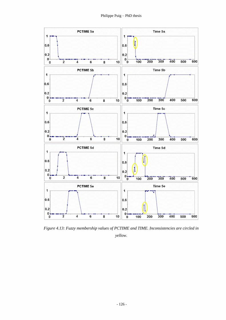
Philippe Puig – PhD thesis
- 126 -
Figure 4.13: Fuzzy membership values of PCTIME and TIME. Inconsistencies are circled in
yellow.

Philippe Puig – PhD thesis
- 127 -
Figure 4.14: Fuzzy membership values of all input variables (except TIME) for class 5a.
None allows to derive a membership function similar to PCTIME 5a.

Philippe Puig – PhD thesis
- 128 -
Clusters of remaining variables plotted for the first of the 5 memberships considered
here are displayed in Figure 4.14. Compared with PCTIME, these 13 plots are very
chaotic. They display inconsistent memberships across the whole range of values.
Results displayed in Figure 4.14 for the first membership function of all variables do
not warrant further efforts.
4.3.3 Discussion
The interpretation of Figure 4.13 and 4.14 leads to a simple conclusion: predicting
how much time an elephant seal spends in one 300 km x 300 km is impossible on the
basis of the 13 environmental predictors considered. Bradshaw et al. (2004) conclude
“In contrast to other studies …, our results suggest that even more complex, non-
linear models still fail to provide a strong predictive framework for apex predator
foraging at coarse spatial scales” (Bradshaw et al., 2004; p. 1021). A detailed
analysis of this statement is outside the scope of this thesis, yet some aspects of this
statement deserve further consideration.
Bradshaw et al. (2004) spent a great deal of time and effort processing a very diverse
dataset to investigate relationships between oceanographic variables and the
behaviour of elephant seals. They relied on Generalised Linear models (GLM) and
Generalised Additive models (GAM) to identify which of the variables considered
could drive elephant seals foraging patterns. The approach they adopted is supported
by Guisan et al. (2002) who researched the roles of GLM and GAM in ecological
modelling. Guisan notes however that GLM and GAM “…implicitly incorporate
biotic interactions and negative stochastic effects … that can change from one region
to another. This can make models fitted for the same species, but in different areas
and/or at different resolutions, difficult to compare ... Hence, the predictive
capability of such models is frequently low…” (Guisan et al., 2002; p. 91). These are
serious limitations as the interpretation of Bradshaw et al. (2004) relies on
oceanographic data averaged within grid cells varying in size between 9 km x 9km
(ocean colour/chlorophyll α) and 25 km x 25 km (sea-ice concentration). They
statistically determine the ideal grid cell size for their interpretation to be 300 km and

Philippe Puig – PhD thesis
- 129 -
consequently resampled all their data to that scale. Defining an ideal spatial
aggregation of measurements of these variables in relation to the problem
investigated is difficult. Their 300 km oceanic grid cells, although statistically the
best compromise, may still be too coarse. As a result of this considerable resampling,
interpretation of the data probably suffers from the modifiable areal unit problem
(MAUP) caused by scale and zoning effects (Wong and Lee, 2005). Once averaged
across 300 km grid cells, one can easily imagine that characteristic signatures of
preferred elephant seals feeding grounds will have a negligible influence on the
average value of all variables in the corresponding cell. In addition, as stated by
Bradshaw (personal communication), dealing with a small sample of intelligent
mammals adds an elusive variable: their “personality”. The latter is probably
impossible to model when dealing with wild animals. This element alone has the
potential to make any kind of predictive modelling of their foraging pattern very
difficult. Ultimately, modelling results obtained by Bradshaw et al. (2004) prove
inconclusive.
So, what is the contribution of fuzzy rule-based modelling to Bradshaw et al.‟s
(2004) study? On the basis of a completely different approach, fuzzy rule-based
modelling supports Bradshaw et al.‟s (2004) finding. The foraging patterns of the
elephant seals considered in this study cannot be predicted from the available dataset.
This lack of predictive capability does not therefore appear to be related to the
modelling methodology adopted by Bradshaw but to the dataset itself. No statistical
assumption or simplification underpins the fuzzy rule-based model. Compared with
GLM and GAM, fuzzy rule-based modelling appears to be a blunt tool. This may be
precisely its greatest quality in GIS/spatial modelling of ecological data. A large
dataset can be rapidly explored to decide if a detailed statistical investigation may be
warranted. If during the identification phase of a fuzzy rule-based model no input
variable appears capable of explaining the output variable there is little chance that a
statistical predictive model can be created. A “sentinel” variable such as TIME in
this study reminds the user of what can be expected when one an input variable is
highly correlated the output.

Philippe Puig – PhD thesis
- 130 -
Fuzzy rule-based modelling can clearly help investigate the suitability of large and
complex datasets to the development of statistical predictive models. This represents
a considerable contribution to GIS modelling both in terms of better allocating time
spent on advanced statistical techniques and in casting some light on otherwise
inconclusive outcomes.
Summary
Two important applications of fuzzy logic to predictive modelling in GIS are
reviewed in this chapter. The first application deals with the classification of
categorical data described by ratio variables. The second application focuses on the
rapid development of predictive models from small datasets of high dimensionality.
The classification model is demonstrated through the classification of Fisher‟s iris
dataset. Four flower metrics are used to differentiate between three varieties of iris
flower: setosa, versicolor and virginica. These metrics are petal length, petal width,
sepal length and sepal width. The identification of the model carried out on 120 of a
total of 150 records shows that sepal width is independent of iris flower variety. This
variable is therefore discarded. For each of the 3 remaining iris metrics, all records of
each variety are represented by one triangular membership function. The resulting
fuzzy rule-based model comprises nine rules. Normalised weightings are calculated
for each rule on the basis of its width and number of associated records. Two models
are implemented: one with rule weightings in Matlab (MathWorks, 1999), the other
without rule weightings in Scilab. Both models are evaluated on the remaining 30
records not used during the identification process. The model with weighted rules
performs best and misclassifies only one flower out of 30.
The rapid development of predictive models from small datasets of high
dimensionality relies on a simplified fuzzy rule-based modelling strategy. This
strategy is implemented on a dataset used by Nakanishi et al. (1993) to introduce a
sophisticated identification technique (Nakanishi et al., 1993). The simplified
identification technique relies on the whole dataset to create a single model.
Segmentation is performed semi automatically by projecting output membership

Philippe Puig – PhD thesis
- 131 -
functions on input variables. Some input variables have membership functions where
records follow a smooth envelope. Erratic envelopes reflect the inability of the
corresponding input variable to follow variations in the output variable. The
simplified strategy concludes that three of the initial five input variables fall in that
category and are therefore discarded. Nakanishi et al. (1993) come to the same
conclusion but his approach is more demanding. Correlation coefficients between
observations and predictions by the two models are compared. Nakanishi et al.‟s
(1993) performs best with a correlation coefficient of 0.99 while the simplified
method scores 0.97.
The simplified fuzzy rule-based modelling method, well suited to the rapid
evaluation of the predictive capability of large multivariate datasets is tested on a
case study of fifty records of foraging patterns of elephant seals in the Southern
Ocean (Bradshaw et al., 2004). Bradshaw et al. (2004) rely on fourteen
environmental variables from varied sources to predict the time spent by elephant
seals in 300km x 300km grid cells. Bradshaw et al.‟s (2004) predictions based on
GLM and GAM models are inconclusive. The identification of the simplified fuzzy
rule-based model shows that none of the environmental variables, on its own, has any
predictive power. Combinations of variables such as flat sea floor in shallow water or
steep slopes in deep water could be considered. Results obtained by Bradshaw et al.
(2004) appear to confirm that, owing to the total lack of predictive capability of all
variables used in his study, no further investigation is warranted. The stark contrast
between the two strategies resides in the simplicity and unambiguous conclusions of
fuzzy rule based modelling method advocated.
This chapter shows that fuzzy logic provides a unified strategy capable of building
classifiers as well as predictive models from multivariate datasets of high
dimensionality. These two typical facets of GIS modelling are well addressed by the
approach advocated in this chapter. Techniques used are not constrained by any
assumption of size or nature of the dataset. The modelling strategy detailed here can
be used on its own or as a precursor to more involved statistical methods, once it has
been independently ascertained that input variables do explain the output variable(s).

CHAPTER 5
KNOWLEDGE DRIVEN FUZZY RULE-BASED
MODELLING

Philippe Puig – PhD thesis
- 133 -
Overview
Concepts of fuzzy logic exposed in Chapter 2 and principles of data driven fuzzy
rule-based modelling established in Chapter 4 provide the foundation required to
introduce the fundamental concepts of knowledge driven fuzzy rule-based modelling.
Knowledge capture is arguably the most important phase in the development of
knowledge driven fuzzy rule-based models. Often called expert systems, these fuzzy
rule-based models have important applications to GIS models developed to improve
the management of fisheries. Expert systems belong to the broader context of
Artificial intelligence (AI). AI (Dubois and Prade, 1998) is mainly concerned with
knowledge-based systems (KBS) and knowledge engineering (KE). KE grew out of
the need to apply sound engineering principles to unreliable early KBSs. KE research
(Chandrasekaran and Josephson, 1997) concentrates now on sharing knowledge and
problem solving methods, or ontologies (Van Heijst et al., 1995; Van Harmelen,
1995), across KBSs. KE is therefore of little relevance to this thesis since it is not
concerned with software development but with practical implementations of
knowledge based predictive models, or expert systems, to address generic needs
(Lehner and Hartmann, 2007). Within this context both knowledge capture and
expert system development related through two case studies.
The first case study is an attempt to model fishing power, an elusive variable that
accounts for the fish catching efficiency of a fishing vessel. Fishing power underpins
the accurate estimation of the productivity of a fishery. Based on the experience of
Mackinson (1999), the focus is on the capture of fishers‟ expert knowledge of fishing
power. Questionnaires on fishing power completed by fishers, their processing and
interpretation are carefully reviewed. An expert system is derived from the data
collected. The limitations of this model and its implication for fishing power
modelling are noteworthy. The second case study is articulated around Cheung et
al.‟s (2005) expert system. Derived from experts‟ knowledge published in the
scientific literature, this expert system provides an insight in the status of two key
commercial species of a fishery in the Northern Territory. Discrepancies between
results obtained and published information demonstrate the relevance of local NRM
fuzzy rule-based expert systems to fishery management.

Philippe Puig – PhD thesis
- 134 -
Other potential applications of expert systems are briefly discussed. Although rarely
explicitly mentioned, GIS models are omnipresent in this chapter. Their interactions
with fuzzy rule-based expert systems are intricate. The resulting modelling synergy
is well suited to environmental systems characterised by a web of spatial and non
spatial interacting processes.
5.1 Knowledge versus data driven fuzzy rule-based modelling
Knowledge and data driven (Dubois et al., 2000) fuzzy rule-based models share the
same rule-based structure and rely on the same principles. The difficulty in data
driven modelling is more in the identification of the model. In knowledge driven
models, often called expert systems, the challenge is in knowledge acquisition.
5.1.1 Expert systems and fuzzy rule-based modelling
What are expert systems? “Expert systems are computer programs that emulate the
reasoning process of a human expert or perform in an expert manner in a domain for
which no human expert exists” (Hall and Kandel, 1992; p.4). Hall and Kandel offer a
useful summary of fundamental aspects of expert systems. Four main structures have
been developed to represent knowledge: rules, semantic networks, frames and
Bayesian networks (Mello and Brown, 1999). Rules adopt the familiar structure
below.
IF premise THEN conclusion
MYCIN (Shortliffe, 1976) was a medical diagnosis system initially applied to the
detection and treatment of bacteremia and meningitis (Duda and Shortliffe, 1983).
Semantic networks are made up of arcs and nodes where nodes represent objects and
concepts while arcs are relations between different types of nodes. CASNET (Weiss
et al., 1978) is an example of a semantic network (Hall and Kandel, 1992: p. 17), was
initially applied to the diagnosis and treatment of glaucomas. Frames describe
specific situations. They may contain data, procedures or pointers to other frames.
PROSPECTOR (Gaschnig, 1982) was a mineral exploration expert system based on

Philippe Puig – PhD thesis
- 135 -
frames. Bayesian networks have been increasingly used to develop knowledge based
predictive models (De Campos and Qiang Ji, 2009; Schubert et al., 2006; Zaarour et
al., 2003). However, applications to real-world problems such as Schubert et al.‟s
(2006) GIS integrated Bayesian network avalanche risk assessment system remain
laborious (Wang, 2004).
The first three expert systems mentioned above are products of the 1970s, a time
when fuzzy logic was still explored to assess what practical applications, if any, it
could have. Imprecision needs to be handled with care in an expert system as queries
from users as well as knowledge provided by experts are uncertain. Uncertainty was
initially translated as probabilities. Experts, however, do not think in probabilistic
terms and this unnatural method of recording vagueness can affect expert
contributions. Early expert systems predate Zadeh‟s seminal paper (Zadeh, 1965).
Expert systems can therefore be based on crisp logic. Hall and Kandel (1992),
however, consider that fuzzy logic improves the performance of an expert system by
better managing imprecision in two domains.
The first domain relates to the relative importance assigned to a piece of information.
Knowledge is traditionally recorded in a probabilistic manner and a statement will be
weighted according to its probability of being correct. The reliability of this
weighting depends on the size of the dataset which in turn decides how
representative the source is. Large datasets are generally rare and weightings are a
common source of imprecision. Fuzzy inference systems, although not immune to
imprecision, address it better than probabilistic systems. Dealing with linguistic
vagueness is the second domain where fuzzy logic is advantageous. Although
alternatives have been used to tackle the inherent vagueness of human language,
fuzzy logic provides an intuitive solution less likely to hinder the capture of human
language.
Fuzzy rule-based expert systems, in their structure and functions, are similar to
previously explored fuzzy rule-based systems. They are however knowledge driven
instead of data driven. Knowledge can be generally treated as data in the sense that
both Mendel (1995, p: 315) and Salski (2006, p: 12) see no difference in the way
numerical data and linguistic statements are processed in fuzzy modelling. When

Philippe Puig – PhD thesis
- 136 -
knowledge represents constraints, instead of positive knowledge or data, neither
Mamdani nor Sugeno-type are suitable. Implicative gradual rules (Ughetto et al.,
1999; Dubois et al., 2003; Jones et al., 2005; Jones et al., 2009) must be used instead.
Implicative rules lead to a different type of inference system which, like the Sugeno-
type inference system, is not considered in this thesis. With the exception of
constraints, there is little difference, conceptually, between data and knowledge
driven fuzzy rule-based models. Practically, knowledge driven models are more
demanding than data driven models as they generally require time consuming, and
therefore expensive, interactions with knowledge providers. There is however, one
substantial difference between them. While data driven fuzzy rule based-models can
be either of Mamdani or Takagi-Sugeno (TS) type, knowledge driven rule-based
models can only be Mamdani type. In a TS model, the output is a mathematical
function of the input (Babuska, 1997). Better suited to engineering applications, TS
type fuzzy rule-based models are incompatible with human knowledge modelling as
their output is a mathematical equation. Only Mamdani type fuzzy inference systems
are discussed in this thesis as they offer a unified approach to predictive modelling in
a raster GIS environment. There is however, no doubt that for specific problems,
involving for instance biochemical systems, TS type fuzzy rule-based models can
perform better. The PhD thesis of Babuska (1996) provides an excellent comparison
of Mamdani and TS type fuzzy rule-based models.
5.1.2 Examples of spatial NRM fuzzy expert system from the fishery industry
Mackinson (1999: p.1) starts with a statement particularly relevant to this thesis
“Since the precise factors that determine changes in structure, dynamics and meso
scale distribution of herring shoals are not well understood, multiple sources of
knowledge are integrated in the framework of a fuzzy logic expert system. Such
work is necessary to develop spatially explicit predictive models needed for
management.” Although he focuses on herring fisheries, his comment can be readily
extrapolated to most NRM domains: fuzzy logic and knowledge are needed for
spatial predictions of natural systems behaviour. Mackinson (1999) developed
Clupex, an expert system built on rules summarising all available relevant
knowledge and scientific data to predict herring shoals properties. Clupex is
characterised by 35 potential inputs and 23 outputs, some of them spatial. Fishers can

Philippe Puig – PhD thesis
- 137 -
view maps of herring shoals along the Canadian coast. Not all rules are fuzzy, but
heuristics that capture knowledge expressed in linguistic expressions play a
fundamental role in this expert system. Clupex was created with Exsys
(http://www.exsys.com), a commercial software mainly aimed at the business world.
The software selected is not necessarily the simplest approach to a typical problem of
natural resources management. Solutions adopted are not transparent and may
implement technical choices better suited to business than to fisheries. However,
three key aspects of this expert system are directly relevant to this dissertation.
Firstly, the development of the knowledge base raises issues common to many expert
systems. Secondly, the role of fuzzy logic in the development of heuristics is a
generic aspect of predictive modelling. Thirdly, the close association between expert
system and mapping can substantially benefit GIS modelling. The development of
the knowledge base is particularly interesting as Mackinson provides revealing
figures. Thirty persons were interviewed: eight fishery scientists, seven fishery
managers, nine fishers and six First Nations informants. Interviews lasted two hours
on average and included open discussions as well as questionnaires. The interview
strategy is articulated around four components. A peer reviewed selection of experts
is the first step. A questionnaire is then devised to combine free and directed
inquiries. The inclusion of “sentinel” questions targeting the truthfulness and depth
of knowledge of interviewees is a crucial safety aspect of this questionnaire. The
review process ensures that all interviewees are satisfied with the integrity of the
information provided once recorded. This thorough, successful yet time consuming
and therefore expensive expert system design methodology needs to be contrasted
with the modest attempt to capture NT fishers knowledge described in this chapter.
The limited success of the latter, developed with minimum resources, should not
therefore be considered as a reflection of the potential of the method.
Cheung et al. (2005) build an expert system of IF-THEN clauses from published
literature on ecological characteristics of marine fishes related to their vulnerability
to extinction under fishing pressure. Predictions of this system match observed
declines. They are an improvement on previous models. Useful both for fishery
management and marine conservation planning, this tool is relevant to tropical
countries where conventional assessment of species extinction vulnerability is
difficult for reasons including lack of data on local population dynamics and high

Philippe Puig – PhD thesis
- 138 -
species diversity. Traditional knowledge of life histories and ecological
characteristics as well as existing databases can provide useful surrogates. One
readily accessible source of information is FishBase, a professional reference online
database of multilingual information on more than 30,900 species of fish edited by
Froese and Pauli (2008). Vagueness and uncertainty, however, are inherent to much
information available on fish biology and ecology as demonstrated later in this
chapter. Fuzzy rule-based systems are well suited to the interpretation of this data.
Cheung‟s expert system was validated on data from the North Sea, Fiji and the
International Union for Conservation of Nature (IUCN) list of threatened species.
Both Mackinson and Cheung developed their fuzzy expert system at the University
of British Columbia (UBC) currently considered by many as the leader in fishery
research. UBC‟s ongoing interest in the application of fuzzy logic to fisheries
management is a strong indication of its potential in a highly spatial domain where
the need for improved management strategies is particularly urgent if dwindling fish
stocks are to be preserved.
5.2 The need to capture human knowledge
This section provides some background on the rationale underlying the first case
study: the development of a fuzzy rule-based expert system of fishing power.
5.2.1 The example of fishing power in the NT
Fisheries rely on a large number of biological, geographical and economical
variables. Fishery scientists are increasingly aware of the benefits of fuzzy logic for a
number of reasons. They are increasingly concerned by the growing evidence that
traditional statistical methods may not be best suited to generate alarm signals
susceptible to protect fish stocks. The demise of the Atlantic cod fishery is a well
known example of a number of cases which fuel their concern. Fishery scientists are
aware of the need to translate unrecorded traditional knowledge into mathematical
models that will improve natural resource management. They need as well, the
flexibility to incorporate particularly elusive variables such as fishing power. The

Philippe Puig – PhD thesis
- 139 -
rest of this chapter gives an account of a study stemming directly from these three
considerations.
Catchrecorded = Catchpotential Fishing Effort Fishing Power Equation 5.1
Let us now focus on fishing power. The catch of a fisher or a fishing vessel, and
ultimately the production of a whole fishery, needs be adjusted to allow comparisons
across a fishery. The expression of the adjusted catch needs to take into account all
parameters that explain systematic discrepancies between catch recorded by boats
fishing in the same location, at the same time, the same species. Mathematically the
problem can be defined by Equation 5.1 above. The five variables in this equation
are defined as follows. The amount of fish caught by the fishers is represented by
Catchrecorded expressed in kg or T of fish. The suitability of the marine environment to
harvesting the species considered is captured by Catchpotential. Fishing Effort is the
product of the time spent fishing by the number of units of fishing gear (trap, hook,
line). Fishing Power incorporates a number of loosely defined parameters which put
together explain why two different fishing vessels targeting the same species under
the same conditions will not catch the same quantity of fish. An environmental
constant is defined locally to account for variations in catch records due to weather
as well as seasonal and climatic factors including El Niño/La Niña cycles.
The definition of Fishing Power suggests that this variable is difficult to evaluate.
Fishery scientists are still grappling with this concept. Marchal et al. (2006) use a
statistical approach based on the GLM. Fishing power, being so difficult to define, is
generally included in fishing effort. Fishing effort thus becomes unpredictably
variable. Marchal‟s (2006) paper suggests that even sophisticated statistics cannot
circumvent a lack of crucial information and that some of the apparent stochastic
variations observed may have a deterministic cause. Fishing power is a typical
product of human language: an accurate definition of a vague concept. The relevance
of this variable cannot be ignored because without effectively accounting for fishing
power, information important to fishery management is unavailable. For instance,
effect of changing a mix of new and traditional technologies in a fishery cannot be
predicted. Discrepancies between observed and predicted productivity, without
knowledge of fishing power, is difficult to interpret. Australian fisheries appear to be
progressively moving away from prohibitively expensive independent records. They

Philippe Puig – PhD thesis
- 140 -
need a reliable assessment of fishing power to meaningfully compare catch records
provided by fishers. The Timor Reef case study presented here is particularly
relevant to the Australian context as well as the European situation reflected by
Marchal (2006).
The Timor Reef Fishery (TRF) displayed in Figure 5.1, located on the edge of the
continental shelf, benefits from a unique combination of drowned terrestrial
topography and seafloor geomorphology characteristic of intense bacterial activity
associated with oil seepage. As a consequence this zone is particularly attractive to
both the fishing and the oil industry. For these reasons, during the last two decades, it
has been the focus of a level of scientific scrutiny without precedent in Northern
Australia. Research project Fishery Research Development Corporation (FRDC)
2005/047 focused on improving the management of this fishery. This project, funded
by the FRDC, an Australian federal fisheries research organisation, included an
initial investigation of fishing power. This study, although not spatial as such, has a
direct bearing on the spatial definition of the very restricted high productivity zone of
the TRF displayed in Figure 5.2. Fishery productivity evaluation in NT waters at
present only relies on catch records provided by fishers divided by fishing effort.
Fishing effort is calculated by multiplying the number of units of a specific fishing
gear (drop line or fish trap here) by the time spent fishing at the recorded location.
Catch records used to create Figure 5.2 are only adjusted for fishing effort. They
should as well be compensated for variations in boat, experience of the skipper and
the crew all captured in fishing power. Accounting for the latter allows management
to map productivity more accurately. This in turn facilitates the investigation of
variations in production and helps refine maps of productivity similar to Figure 5.2.
Such maps are fundamental to monitor fluctuations in productivity and ultimately the
very survival of fisheries.
Figure 5.1: The Timor Reef Fishery, in red, is the closest fishery to Darwin (black circle).

Philippe Puig – PhD thesis
- 141 -
Figure 5.2: Map of the productivity of the TRF. Dark orange areas show the zones of highest
commercial value derived from the GIS analysis of catch records plotted on digital maps of
geomorphic units and bathymetry. Yellow represents zones of lowest value. This map, based
on the interpretation of 10 years of catch records (Lloyd and Puig, 2009) ignores fishing
power.
What follows is the first step in establishing a model of fishing power derived from
fishers‟ knowledge. Mackinson‟s work, previously mentioned, is a useful benchmark.
However, this case study relies on a much smaller number of informants. Although
undesirable, this situation is more representative of applications outside academia
where critical material constraints, often cost related, prevail. Here, an additional
difficulty is the small number of experienced fishers.
5.2.2 Capture of human knowledge
Cheung et al. (2005) built their fuzzy expert system from peer reviewed scientific
literature, a source of captured knowledge. Their model is a useful tool for fishery
scientists. There is little doubt that their approach would be equally applicable to
other NRM domains. In this instance, however, scientific literature is unlikely to be
suitable as local models need to be developed from local knowledge. In many
regions of the world there is currently a domain of human knowledge, outside
academia, which is of growing interest to scientists: traditional ecological knowledge
(TEK) is a subject of much interest in NT environmental research circles (Smith,
2008; Smith, 2009). Unfortunately the adoption of a suitable generic interpretative
framework has not received much attention. This case study can be easily adapted to

Philippe Puig – PhD thesis
- 142 -
a wide range of purpose specific applications to predictive modelling based on
expertise that is independent of the technical or cultural background of the
informants.
5.3 Modelling fishing power from fishers’ knowledge
The method of recording experts‟ knowledge used here was derived from a
frequently cited study by Chameau and Santamarina (1987). They compared four
elicitation methods, described in section 2.5.2, and based their evaluation on
questionnaires distributed to 22 professors and graduate students considered either as
measurement instruments or repositories of knowledge. The fourth method of expert
knowledge capture described, i.e. pair wise comparison, is implemented in Chapter 3,
within the AHP, to develop a GIS of prawn farming site suitability. Both experts who
participated in this case study concluded that pair wise comparison is effective but
tedious. The interpretation of the results is taxing. In contrast, the following case
study of capture of fisher‟s expert knowledge relies on the second elicitation method,
interval estimation (Chameau and Santamarina, 1987), considered the best of the four
methods listed. Fast and simple, interval estimation has lowest fuzziness. However,
the method is only considered to be reliable if a minimum of 5 informants are
surveyed, which may be a major limitation when experts are considered.
Chameau and Santamarina (1987) drew three practical conclusions from their study.
Firstly, the larger the scale given to informants is, the wider the discrepancies
between informants‟ views and the fuzzier their answers are. Secondly, scales no
larger than 10 perform best. Thirdly, informants preferred the interval estimation
method.
5.3.1 Fishing power of fishing units of the Timor Reef Fishery
The Timor Reef Fishery is characterised by no more than twelve operating fishing
vessels at any given time since its creation in 1989. The number of experienced
fishers is even smaller as few of the original fishers are still fishing these waters.
Fishers who participated in this survey were very busy and therefore rarely available.

Philippe Puig – PhD thesis
- 143 -
Four experienced fishers found the time to participate in this activity which consisted
in a short presentation on the rationale of the study and the subsequent process of
filling in the questionnaire. Questions and forms were prepared by fishery research
scientists of the Northern Territory Government. The questionnaires reflect their
views on what contributes to the power of a fishing unit defined as a vessel. The
suitability of the questionnaire to the task is not relevant to the present discussion
which focuses on processing the information recorded. There is no doubt, however
that the design of the questionnaire itself deserves careful consideration.
The questionnaire relies on the familiarity of the informants with the subject matter.
All fishing vessels are known to the informants. Their specifics, however, are
detailed to enable these experts to assess the contribution of each element on what
they know to be the performance of the overall fishing unit. A fishing unit
incorporates crew and equipment. Eleven local vessels were selected and
documented in detail. Chameau and Santamarina‟s (1987) interval estimation was the
technique adopted for this study of fishing power. The survey consisted in selecting a
range of numbers between 0 and 10 that best described the fishing power of each of
seven groups of features for each of eleven vessels operating in the TRF. The lowest
power corresponded to 0 and the highest to 10. Fishers were encouraged to select a
range of values when no single number appeared appropriate. The seven feature
classes considered are listed in Figure 5.3 are dimensions, engines, ice-maker,
product storage, electronics, fishing gear and crew. Characteristics of the eleven
vessels were detailed, for each of the seven classes above, in five forms. Figure 5.3
shows the form for vessel 4 and 5. Once the fishing power of all seven classes of
features were evaluated, fishers had to assign the fishing power they expected the
corresponding vessel.
Between five and ten informants were to participate in the survey. Only four actually
did. Only two fishers completed their questionnaires correctly. Due to the limited
duration of project FRDC 2005/047 and the small pool of experienced TRF fishers,
there was no opportunity to approach additional fishers. Despite its limitations, this
survey offers a useful insight in four important aspects of knowledge acquisition and
processing: evaluation of questionnaires, rescaling answers, translation of answers
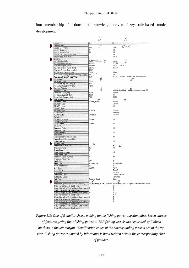
Philippe Puig – PhD thesis
- 144 -
into membership functions and knowledge driven fuzzy rule-based model
development.
Figure 5.3: One of 5 similar sheets making up the fishing power questionnaire. Seven classes
of features giving their fishing power to TRF fishing vessels are separated by 7 black
markers in the left margin. Identification codes of the corresponding vessels are in the top
row. Fishing power estimated by informants is hand written next to the corresponding class
of features.

Philippe Puig – PhD thesis
- 145 -
5.3.2 Critical evaluation of knowledge data
The following codes are used in Figure 5.4 which displays records directly derived
from questionnaire sheets similar to the sample displayed in Figure 5.3.
FP = fishing power of the whole fishing unit IM = ice-maker;
DI = dimensions of vessel PS = product storage
EN = engines EL = electronics;
FG = fishing gear
Average ratings for each category are first calculated to compare the views of these
two experts. Results are plotted in Figure 5.4. Estimates of fishing power from
Informant 2 are systematically higher. Rescaling the information provided is
necessary to avoid unnecessarily widening membership function. As informants are
used as measuring instruments to measure the quantity fishing power, this rescaling
is equivalent to recalibrating measuring instruments before a survey. The intention is
not to modify the views of the experts but merely to make comparisons more
meaningful.
One important role of graphs in Figure 5.4 is to verify that variables identified by NT
Government fishery scientists to produce the questionnaire displayed in Figure 5.3
are relevant. Although fishers were consulted before completing the questionnaire
form, one of the seven input variables supposed to explain the fishing power of each
TRF fishing vessel should have been discarded. “Ice maker” recorded nineteen
estimates of 0 fishing power out of a total of twenty estimates. The two experts
indicated through their estimates that “Ice maker” does not contribute to the overall
fishing power of a TRF vessel. Therefore, this variable is removed from the model.
Most records reflect a lack of contrast in the dataset.
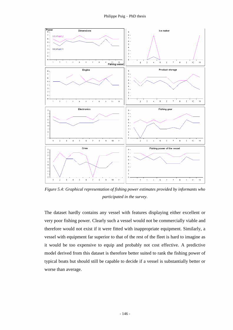
Philippe Puig – PhD thesis
- 146 -
Figure 5.4: Graphical representation of fishing power estimates provided by informants who
participated in the survey.
The dataset hardly contains any vessel with features displaying either excellent or
very poor fishing power. Clearly such a vessel would not be commercially viable and
therefore would not exist if it were fitted with inappropriate equipment. Similarly, a
vessel with equipment far superior to that of the rest of the fleet is hard to imagine as
it would be too expensive to equip and probably not cost effective. A predictive
model derived from this dataset is therefore better suited to rank the fishing power of
typical boats but should still be capable to decide if a vessel is substantially better or
worse than average.

Philippe Puig – PhD thesis
- 147 -
5.3.3 Rescaling knowledge data
Here, rescaling the data consists in changing the origin only. Modifying the unit of
measurement could be considered in principle, however such drastic modification of
the original data should only be considered after careful investigation as it may cast
doubts on the reliability of the model.
Table 5.1: Fishing power estimates collected with the questionnaires are recalibrated to
account for informant’s systematic bias.
As fishers are more likely to agree on the overall fishing power of vessels than on the
power of their parts, Table 5.1 focuses on the average estimated fishing power of the
11 vessels. The first informant‟s estimates are close to the expected value of 5, while
the second informant‟s estimates are higher. For reasons previously outlined, both
datasets will be adjusted to obtain an average fishing power of 5 which is the centre
of the scale [0,10]. Both informants rank the “Ice Maker” as the least important
contributor to the fishing power of the vessel. This variable is consequently removed.
Table 5.2 contains the rescaled fishing power estimates used to derive a fuzzy rule-
based model.

Philippe Puig – PhD thesis
- 148 -
Table 5.2: Rescaled fishing power estimates. Values in Table 5.1 (column FP) are adjusted
to obtain equal averages of 5. Identical adjustments are added to corresponding arrays in
Table 5.1 to obtain all adjusted estimates. The “Ice Maker” IM variable is removed. Grey
cells are ignored in calculations as they merely reflect the absence of answer.
5.3.4 From estimates to membership functions
Data from Table 5.2 is merged into Table 5.3 to calculate for each variable the
minimum, average and maximum estimate fishing power. These statistics, displayed
in Table 5.3, become the coordinates of the corresponding triangular membership
functions in the fuzzy rule-based model of fishing power. From Table 5.3 we can
readily define the following seven triangular membership functions.
fishing power of vessel (FP) FP-M with coordinates (3.9, 5, 5.9)
fishing power of dimensions (DI) DI-M with coordinates (3.3, 4.6, 5.9)
fishing power of engine (EN) EN-M with coordinates (3.3, 4.5, 5.9)
fishing power of product storage (PS) PS-M with coordinates (2.9, 4.8, 5.1)
fishing power of electronics (EL) EL-M with coordinates (3.9, 5.3, 5.1)
fishing power of fishing gear (FG) FG-M with coordinates (2.9, 4.2, 5.1)
fishing power of crew (CR) CR-M with coordinates (2.9, 4.9, 5.1)

Philippe Puig – PhD thesis
- 149 -
The triangular membership functions above correspond to medium fishing powers.
They associate input fishing power estimates for the 6 input variables DI, EN, PS, EL,
FG and CR to output fishing power FP.
Table 5.3: Coordinates (a, b, c) of triangular membership functions for medium values of
fishing power of all variables. a, b, c correspond to minimum, average and maximum values,
respectively. Rows with incomplete information (row 2 yellow and row 7 blue) are ignored.
Membership functions for Low and High power membership functions can be easily
derived from Medium membership functions. The technique, demonstrated in Figure
5.5, stems from a principle established in Chapter 2: membership values should add
up to one.

Philippe Puig – PhD thesis
- 150 -
Figure 5.5: Trapezoidal membership functions of low (blue), medium (orange) and high (red)
fishing power of fishing units.
Trapezoidal fuzzy numbers TaFN and triangular fuzzy number TiFN define all three
membership functions of the fishing power of TRF fishing units. They are listed
below.
FP Low fishing power = FP-L TaFN (FP-L) = (a, b, c, d) = (0, 0, 3.91, 5)
FP Medium fishing power = FP-M TiFN(FP-M) = (e, f, g) = (3.91, 5, 5.91)
FP High fishing power = FP-H TaFN = (h, i, j, k) = (5, 5.91, 0, 0)
The same reasoning is extended to the six input variables DI, EN, PS, EL, FG, CR.
Trapezoidal and triangular fuzzy numbers of all membership functions are listed in
Table 5.4. The information in Table 5.4 is entered into Scilab (Campbell et al., 2006)
to develop a fuzzy-rule based model of fishing power using the Scilab settings
displayed in Figure 2.14.

Philippe Puig – PhD thesis
- 151 -
Table 5.4: Coordinates of all membership functions necessary to create an initial fuzzy rule-
based model of fishing power for the TRF fishery.
Figure 5.6: Graphical representation in sciFLT of all membership functions of input
variables DI, EN, PS, EL, FG, CR. Blue triangular membership functions are derived from
questionnaires while black and green trapezoidal membership functions are inferred.

Philippe Puig – PhD thesis
- 152 -
Table 5.5: Rules defining logical associations between estimates of fishing power for all
inputs DI, EN, PS, EL, FG, CR and the fishing power FP of the whole fishing unit.
Six triangular membership functions are derived from informant estimates: one for
each of the six categories of features responsible for the fishing power of a fishing
unit. Twelve additional membership functions are generated. These twelve additional
membership functions simply exploit the previously mentioned “complement to 1”
property which states that throughout the range of output values of the model, the
sum of memberships for all output values is equal to 1. The simplest membership
functions capable to achieve this role are the trapezoidal functions that flank each
triangular membership function to its left and right (Figure 5.6). Out of a total of
twenty one membership functions displayed in Figure 5.5 and 5.6, only one third, the
triangular membership functions, rely on fisher‟s expertise. The predictive model of
fishing power comprises eighteen rules, R1 to R18, displayed in Table 5.5. They are
generated from these twenty one membership functions by assigning the input
membership functions Low, Medium and High fishing power of each feature of a
fishing unit to the corresponding output membership function of fishing unit.
Although these 18 rules have the same weighting by default, it is clear that all rules
based on trapezoidal membership function are less reliable as they are not based on
hard evidence. The model is evaluated by comparing the estimates of fishing power
by the two experts fishers to the prediction of the model created from the same
estimates. Scattered predictions displayed in Figure 5.7, and a low correlation
coefficient of 0.54, reflect the poor predictive capability of the model.

Philippe Puig – PhD thesis
- 153 -
Figure 5.7: Plot of predicted against observed fishing power of fishing units.
5.3.5 Discussion
This study of fishing power is based on only two informants. Chameau and
Santamarina (1987) recommend a minimum of five informants. The main limiting
factor was the availability of reliable informants. This constraint is likely to be a
systematic difficulty of knowledge surveys. Knowledge driven fuzzy rule-based
models may initially have to rely on numbers of informants smaller than the
prescribed minimum. Information could be acquired through successive surveys
leading to an incremental model development process likely to improve the poor
predictive capability of the initial model.
The limited predictive capability of this model can be explained by the lack of
information in the lower and upper part of the range of values of fishing power
considered. Figure 5.6 shows that any input that does not exactly correspond to the
apex of a triangular function fires a well defined triangular membership function and
a poorly defined trapezoidal membership function. Trapezoidal membership
functions in this model do not reflect hard evidence. They are merely derived from
the triangular membership functions themselves. The stronger the contribution of
trapezoidal functions in this model, the poorer the predictions. A consequence is the

Philippe Puig – PhD thesis
- 154 -
presence, in the predicted dataset, of values of fishing power both lower and higher
than those observed.
The previously mentioned lack of hard evidence to support the trapezoidal
membership functions of this model, results from a training dataset of eleven
operating fishing vessels all with average fishing power. This lack of contrast is
undesirable from a modelling point of view but understandable within the context of
this survey. Operational vessels are unlikely to display either low or high fishing
power. In the first instance they would be uneconomical as low fishing power would
imply little income. In the second instance they would be too expensive to fit.
Fishing power is therefore only likely to show some contrast if vessels from different
origins are included in the survey. Australian neighbours such as Indonesia would
typically benefit from estimates of fishing power if they intended to merge catch
records reported by traditional fishers and vessels similar to those operating in the
TRF.
The knowledge elicitation method demonstrated here is well suited to the
development of knowledge driven fuzzy rule-based models. The first step of the
model identification process consists in minimising the vagueness of the available
information through the range of values selected. To do so records are rescaled, if
necessary, after checking the consistency of the informants‟ views. Finally irrelevant
variables indirectly identified by the informants are eliminated. Weightings were not
implemented in this model as informants had similar views and were sure of their
answers. Weightings could play an important role in improving the performance of
this fuzzy rule-based by giving more importance to triangular membership functions.
However, weightings would thus give more credibility than it deserves to a model
which would still be based on a restricted range of data. As it stands there is no doubt
that this model is simplistic as it relies only on two informants while five is
considered as the minimum. This technique needs therefore to be validated on a
larger, more representative dataset.
Reflecting on the purpose of estimating fishing power, TRF management can rely on
the map of productivity displayed in Figure 5.2. Fortunately, this map is not distorted

Philippe Puig – PhD thesis
- 155 -
by catch records from fishing units with different fishing powers. This situation is
likely to prevail in small isolated fisheries characterized by a stable fleet.
5.4 Implementation and applications of a functional fuzzy rule-
based expert system
Exploring the development of a knowledge driven fuzzy rule-based expert system in
the first part of this chapter provides a good understanding of a number of
fundamental issues likely to affect many similar expert systems. Mackinson‟s (1999)
and Cheung‟s (2005) models, introduced in section 5.2, originated from the rapidly
growing needs of fisheries to incorporate human knowledge in their modelling
strategies. Clupex, created by Mackinson (1999), relies on fishers‟ knowledge to
develop in Exsys a predictive model of herring shoals. Cheung et al. (2005) tapped
researchers‟ knowledge in scientific journals to create an expert system capable of
predicting the vulnerability of commercial fishes to fishing pressure on the sole basis
of biological parameters. Unfortunately, owing to the proprietary nature of the
software used by Mackinson, Clupex cannot be investigated without purchasing
Exsis. Cheung et al. (2005) on the other hand published all the parameters of his
model developed in Excel (Kelly, 2006) using very standard fuzzy rule-based
modelling techniques. Cheung et al.‟s (2005) model was therefore easy to replicate
in Scilab.
Cheung et al.‟s (2005) reliance on Excel is worth noticing. Such ubiquitous and
affordable software is well suited to experimental fuzzy rule-based modelling.
Appendix 2 describes Exfis (Excel fuzzy inference system) a similar application of
Excel functionality. Exfis was an excellent opportunity to experiment with many
fuzzy modelling concepts at an early stage of this thesis. The open source freeware
Scilab (Campbell et al., 2006), however, was ultimately preferred as models were
developed for commercial applications incompatible with the use of a student version
of Matlab (MathWorks, 1999). As Scilab (Campbell et al., 2006) emulates Matlab,
all knowledge of Matlab is easily transferable into Scilab. The implementation of
Cheung‟s model, described here, is completely software independent. Good
graphical representation of all membership functions and clear definitions of all

Philippe Puig – PhD thesis
- 156 -
variables and rules are provided. Membership functions coordinates derived from his
published figures were easily imported into Scilab. The model was then tested on the
two prime target species of the TRF. The sustainability of catches of the first species,
the Goldband snapper (Pristipomoides multidens), were very controversial.
Accessing views of international experts through Cheung‟s expert system was timely
as interest from oil and gas exploration was gathering momentum in the Timor Reef
area. Input parameters were emailed to Cheung who confirmed (see Appendix 4) the
results described here. Later, the extinction vulnerability of the Red Emperor
(Lutjanus sebae), second most sought after species of the TRF, was calculated as
well.
5.4.1 Description of Cheung’s expert system
Cheung et al.‟s (2005) expert system comprises eight weighted input variables and
one output variable. The eight input variables are: maximum length, age at first
maturity, longevity, von Bertalanffy growth parameter K, natural mortality rate,
fecundity, strength of spatial behaviour and geographic range. The output variable,
level of intrinsic extinction vulnerability to fishing, is defined by 4 membership
functions. Maximum membership value is 1. Cheung (2005) tested their model on
159 marine fishes with complete records of life history and ecological characteristics
extracted from FishBase, a reference online database of multilingual information on
more than 30,900 species of fish edited by Froese and Pauli (2008).
Cheung et al.‟s (2005) evaluation focused on five aspects of the model. The
sensitivity of the model to the removal of the various input variables was tested along
with the rules‟ weightings. The validity of vulnerability estimates was compared with
known historical abundance trends. The goodness-of-fit of the test statistics
reflecting the predictions accuracy was checked. Predictions obtained from two
surrogates of extinction risks, maximum length and age, matched broad model
outputs. Advantages of the fuzzy rule-based model over an identical Boolean model
were demonstrated.

Philippe Puig – PhD thesis
- 157 -
Cheung et al. (2005) made a number of observations. The predicted intrinsic
vulnerabilities are insensitive to threshold values. Deviations in the output, generally
small when individual inputs were eliminated, increase with the number of input
variables removed. Intrinsic vulnerabilities predicted by the expert system are
significantly better than those from the two surrogates maximum length and age at
first maturity. Once fuzzy sets are replaced by classical sets there is no correlation
between predicted intrinsic vulnerability and population trends. Information on reef
fish aggregation greatly improved the system performance for Fiji‟s reef species.
Eliminating fecundity causes little variation in expert system performance. Intrinsic
vulnerability is a lot more dependent on maximum length and age at first maturity.
The considerable contribution of this expert system fishery management is its ability
to predict extinction vulnerability for species indirectly targeted by commercial
fishing for which no stock assessments or population trends exist. This expert system
estimated, from a dataset of 900 species of fish, the intrinsic vulnerability (Morato et
al., 2006) to be higher among seamount species than among non seamount species, a
result supported by the sudden demise of a number of seamount fisheries. Cheung
and his colleagues concede however that additional factors should be integrated with
intrinsic vulnerability to provide an overall assessment of risk of extinction.
5.4.2 Implementation of Cheung’s expert system in Scilab
The actual implementation of Cheung‟s et al.‟s (2005) expert system does not consist
in simply recreating an expert system. The original model has to be truncated to
remove rules based on variables for which no local data is available. This situation,
common in real world resource management applications, demonstrates a substantial
advantage of fuzzy rule-based models over equation based models more difficult to
adapt to local needs.
Cheung et al. (2005) provides clear and complete directives sufficient to build his
expert system from figures and explanations provided in his paper. All input and
output membership functions in Figures 5.8, 5.9 and 5.10 have been recreated in
Scilab from coordinates directly read from figures in his paper.

Philippe Puig – PhD thesis
- 158 -
Figure 5.8: First 4 input variables maximum body length, age at first maturity, von
Bertalanffy growth parameter K, Natural mortality rate and their corresponding
membership functions.
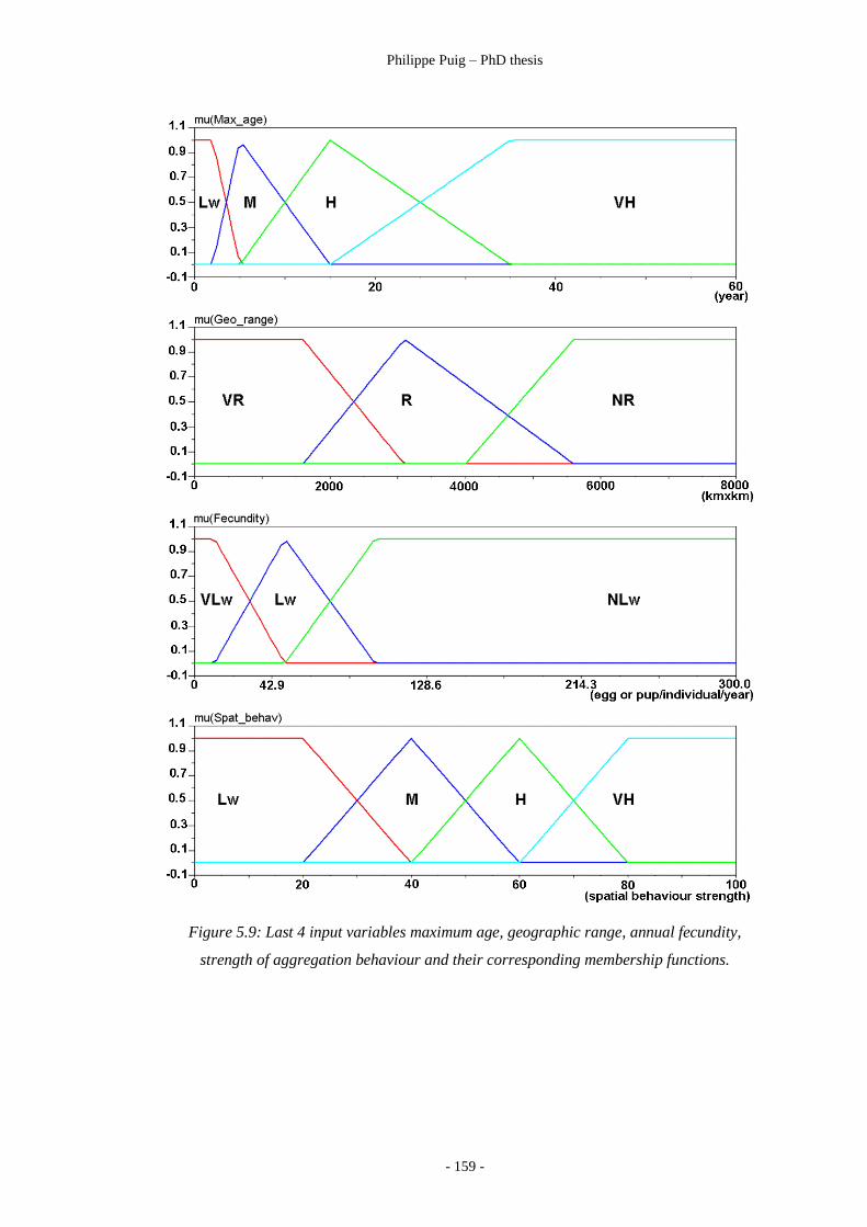
Philippe Puig – PhD thesis
- 159 -
Figure 5.9: Last 4 input variables maximum age, geographic range, annual fecundity,
strength of aggregation behaviour and their corresponding membership functions.

Philippe Puig – PhD thesis
- 160 -
Figure 5.10: Output variable Intrinsic vulnerability of fish species to fishing pressure and its
4 membership functions measured on an arbitrary scale of 1 to 100. The value of highest
vulnerability is 100.
Only the first eighteen of the twenty five rules listed in Cheung‟s paper, written in
Scilab, are displayed in Table 5.6. Note that Cheung‟s original model contains only
two rules including fecundity. The third rule, based on membership function NLw
displayed in Figure 5.9, does not appear in his model. The influence of this rule on
the model is negligible as the fecundity of most species fall in the Not Low
membership function. Rules relying on geographic range and spatial behavior do not
appear in Table 5.6 as no information on these two variables was available for the
two species of the Timor Reef fishery considered here. Rules related to these two
variables were therefore removed from the model.
Table 5.6: All rules from Cheung’s (2005) expert system retained in the model of fish
vulnerability to fishing pressure implemented in this chapter.

Philippe Puig – PhD thesis
- 161 -
Once built in Scilab, using the sciFLT toolbox, Cheung‟s model is used to calculate
the intrinsic vulnerability to fishing pressure of two important commercial species of
the Timor Reef fishery. Biological parameters required by the model were provided
for Goldband snapper (Pristipomoides multidens) and Red Emperor (Lutjanus sebae)
by Julie Lloyd, then a senior marine biologist with the Fisheries Department of the
Northern Territory Government. Although information of this nature can be
downloaded from FishBase, local knowledge is fundamental as will be argued in
section 5.10.3.
Table 5.7: Vulnerability to fishing pressure of Goldband snapper and male (M) and female
(F) Red Emperor.
The resulting vulnerability values (Table 5.7) indicate that the Goldband snapper
vulnerability to fishing pressure is highest. Male and female Red Emperor are
characterised by different parameters. The highest of the two values should be
retained as it provides a more conservative estimate of the resilience of the Red
Emperor to fishing pressure. The intrinsic vulnerability of a species to fishing
pressure is an estimate which varies with the geographical source of the information
fed into the model. Figure 5.11 is a useful visualisation of the effect of variations in
maximum length and age of the Goldband snapper on its intrinsic vulnerability. To
generate Figure 5.11 in Scilab, all but 3 variables displayed in Table 5.5 are kept
constant. Figure 5.11 shows how at the point in space (First_Mat, VBGF_K,
Nat_Mort, Fecundity) defined by values for Goldband snapper in Table 5.7,
variations in Max_Age and Max_L affect its intrinsic vulnerability. If older and
larger specimens of Goldband snapper were captured in the TRF area, the apparent
vulnerability of the species would rise. This observation suggests that FishBase
information needs to be considered carefully.

Philippe Puig – PhD thesis
- 162 -
Figure 5.11: 3D plot showing how maximum length (Max_length on Y axis) and age
(Max_age on X axis) affect the intrinsic vulnerability of Goldband snapper at point (5, 0.23,
0.14, 165000) in the four dimensional space (First_Mat, VBGF_K, Nat_Mort, Fecundity).
5.4.4 Discussion
Results in Table 5.7 support the views of Cheung et al. (2005) that maximum length
appears to be a good predictor of intrinsic vulnerability. Goldband snapper is more
vulnerable than Red Emperor as the maximum length of the former species is larger.
Fecundity plays a minor role and can generally be ignored for one reason at least:
most fish produce more than 100 egg/individual/year and belong therefore to the
NLw (Not Low) membership function as shown in Figure 5.10. FNLw fecundity is
represented by trapezoidal membership function which plateaus for values larger
than 100 egg/individual/year. Fecundity will therefore fail to differentiate between
intrinsic vulnerabilities of the many fishes with fecundity larger than 100. Fecundity
can consequently be ignored in most cases as stated by Cheung (Appendix 4.11).
Spatial behaviour and geographic range were not included in the model because no
information was available. Two advantages of fuzzy rule-based expert systems are
highlighted by this approach. Firstly, their layered structure, where all rules act in
parallel, allows to easily simplify models by switching off variables where they have
the same constant value across all inputs. Secondly, some rules can generally be
removed without completely incapacitating the model. A drop in predictive
capability may be observed but the model remains functional. This represents a

Philippe Puig – PhD thesis
- 163 -
tremendous advantage over more traditional mathematical or statistical models where
even if some variables can be removed from the original equation, numerous
adjustments of the original model may be necessary. In addition to its advantages
over more conventional models, this model proved to be a very useful complement
of FishBase (Froese and Pauli, 2008) to assess the vulnerability of two important
commercial fishes of the TRF: the Red Emperor and the Goldband Snapper.
The Red Emperor can be found in the Indo West Pacific, the Red Sea, East Africa
and as far North as Japan (Froese and Pauli, 2008). A valuable fish in all Tropical
Australian fisheries, this species is characterised by patchy biological information. Its
fecundity is not listed in FishBase. The Goldband snapper and Red Emperor share
the same geographical range. The vulnerability of the former is high and very high
for the latter according to FishBase. These results contradict those in Table 5.7
obtained in Northern Territory waters. Discrepancies between global estimates
provided by FishBase and regional or local intrinsic vulnerability assessment
obtained by Cheung‟s et al’s (2005) fuzzy rule-based expert system highlight a
fundamental role that fuzzy rule-based expert systems can play in most domains of
natural resources management. While global models identify variables to incorporate
in a model, expert systems can generate locally relevant predictions from local data.
Cheung was contacted (see Appendix 4) to confirm the Goldband Snapper
vulnerability in Table 5.7. Cheung found 60.2 instead of 61.4. This value 1.2% lower
than the result displayed in Table 5.7 was initially attributed to differences in
software. Further investigation revealed a flaw in sciFLT (Urzua, 2003)
undocumented although known to its author. Cheung used an Excel (Kelly, 2006)
based computational environment assigning weightings equal to 0.5 to all rules.
Although sciFLT offers the same option to assign weightings to rules, weightings are
not reflected in the output. Urzua ([email protected]) was contacted. He
explained his intention to implement rule weightings in the sciFLT extension for
Scilab 5.x versions. In its current version, however, sciFLT does not support
weighted rules. Weightings remain equal to 1 regardless of the value assigned.
Once the minor discrepancy issue is addressed one may wonder what an intrinsic
vulnerability of 60 actually means? According to FishBase, a vulnerability of 60 is
high. Cheung and al. (2005) quoted in their paper that the ill fated Atlantic Cod, a
Philippe Puig – PhD thesis
- 164 -
sadly emblematic species for all fishery scientists, has an intrinsic vulnerability of 62.
This comparison immediately puts the intrinsic vulnerability of the Goldband
snapper in a more meaningful context for any fishery manager. FishBase intrinsic
vulnerability values, although useful globally, lack the regional or local context of
Cheung‟s expert system outputs.
The contradiction between FishBase vulnerability indices and Cheung expert system
estimates should remind fishery managers that global models, FishBase in that
instance, are poor local predictors. Even when the same modelling principles hold
locally, global estimates may be incompatible with local observations as they rely on
global instead of local statistics. Local observations in absence of historical data
should be considered carefully as low intrinsic vulnerability may simply indicate that
the species has already suffered from fishing pressure. The outcome would be a
decrease in maximum age and length resulting in an apparent decrease in
vulnerability. This may explain why in the TRF the Red Emperor appears less
vulnerable than the Goldband snapper. This intrinsic vulnerability model is a
particularly valuable management tool as it can enable a state like Western Australia,
with fisheries ranging from temperate cool in the south to tropical in the north, to
rank within each fishery their commercial species on the basis of their sensitivity to
fishing pressure. Each fishery could then aim at establishing more realistic quotas by
relying on species vulnerabilities which would be fishery specific.
Summary
This chapter is devoted to the inclusion of human knowledge into fuzzy rule-based
models often called fuzzy rule-based expert systems. Topics covered here do not all
have a cartographic expression. Yet, all can play an important role in the production
of maps instrumental in better managing natural resources. The Timor Reef Fishery
(TRF) provides a backdrop for two case studies which demonstrate two
methodologies relevant to a wide range of NRM contexts. The first methodology
focuses on the acquisition of experts‟ knowledge to build an expert system. The
second methodology consists in implementing an existing expert system to compare
local predictions with preexisting global predictions.
Philippe Puig – PhD thesis
- 165 -
The acquisition of experts‟ knowledge was prompted by the need to improve a GIS
model of productivity of the TRF, a fishery in the Northern Territory. The current
model is based on catch records only compensated for fishing effort. Catch records
need as well to be adjusted for variations in fishing power. The latter, however is a
notoriously elusive variable, easy for expert fishers to estimate qualitatively but hard
to quantify in a systematic and reproducible manner: a typical domain of application
for fuzzy expert systems. The first step in the development of a fuzzy expert system
consists in recording experts‟ knowledge. A number of knowledge acquisition
methods have been documented (Bilgic and Turksen, 2000). Tests carried out by
Chameau and Santamarina (1987) identify the interval estimation method as the most
efficient. This technique was used with the collaboration of TRF expert fishers to
estimate the fishing power of eleven vessels and seven of their characteristic features.
Results from this study reveal that, once rescaled, estimates from informants are
highly correlated. The fishing power of all eleven fishing vessels considered is
average. The experts surveyed discarded one of the seven variables suspected to
affect fishing power. Low, Medium and High fishing power membership functions
are inferred for all six input variables endorsed by the two expert fishers. However,
as the questionnaires only provide information on medium fishing power, the overall
predictive capability of the model is low. This study has four outcomes. Firstly, the
knowledge capture methodology adopted is well suited to the task. Secondly, experts
need to be presented with a variety of information sufficient to explore the full range
of possible values of the output variable which was not possible here. Thirdly, the
minimum number of 5 informants required to create a reliable expert system, as
suggested by Chameau and Santamarina, is a limitation of this technique. Finally, the
current model of productivity of the TRF is more reliable than expected as all fishing
vessels have approximately the same medium fishing power. Despite the restricted
range of fishing power of the training dataset affects the predictive capability of this
model, there is little doubt that this approach is promising. Modelling fishing power
is urgently needed wherever management has to rely on catch records to monitor the
sustainability of fishing practices.
Cheung et al. (2005) describes in detail a fuzzy rule-based expert system developed
entirely from expert knowledge embedded in research literature. The structure of
their model is strikingly similar to that of the model of fishing power previously

Philippe Puig – PhD thesis
- 166 -
described. Cheung‟s et al.„s (2005) model predicts the intrinsic vulnerability of fishes
to fishing pressure on the basis of 8 biological variables. Once implemented from the
detailed description in Cheung‟s et al.„s (2005) paper, this model is used to predict
the vulnerability to fishing pressure of the most important commercial species of the
TRF: the Goldband snapper. Its vulnerability of 61 on a scale of 0 to 100 was
confirmed by Cheung et al. (2005). The Goldband snapper is therefore highly
vulnerable, on a par with the Atlantic cod. Discrepancies between vulnerabilities
provided by online FishBase and Cheung‟s et al.„s (2005) expert system suggest that
local vulnerability of commercial species are inaccurately estimated by FishBase.
Fuzzy rule-based expert systems have two major advantages. Firstly, some variables
can often be ignored without dramatically affecting the model‟s output. Secondly,
fuzzy rule-based expert systems and data driven fuzzy rule-based models share the
same structure detailed in Chapter 4.
Merging fuzzy rule-based expert systems and GIS models into a spatial predictive
system produces a new variety of Geographic Information System with much greater
capabilities as demonstrated by Mackinson (1999) with Clupex. An additional
example is provided by the Timor Reef fishery case studies considered in this chapter.
The expert system of fish vulnerability to fishing pressure devised by Cheung et al.
(2005) has much potential. In a large fishery it could be merged with an existing GIS
model to produce a new type of Geographic Information System. Effects of
environmental changes, species maps of productivity similar to Figure 5.2, and
species vulnerability could all be combined to predict on a yearly basis the ideal mix
of species targeted in each zone of the fishery to maximise both sustainability and
profit.

CHAPTER 6
CONCLUSION

Philippe Puig – PhD thesis
- 168 -
Overview
Chapters 2 and 5 focus on fuzzy rule-based modelling. Chapter 3 explores a radically
different implementation of fuzzy logic. The contrast between Chapter 3 and the
remaining chapters is a reminder of the variety of implementations of fuzzy logic
which lack the wide range of applications, unified framework and credentials of
fuzzy rule-base modelling. Case studies in Chapters 4 and 5 demonstrate that fuzzy
rule-based modelling equips GIS modellers with the same strategy capable to build a
variety of multivariate predictors from experimental data or human knowledge. This
approach leads to directions of research poised to benefit developing countries.
GIS modelling will gain most from combining the sophistication of statistical
methods with the simplicity and versatility of fuzzy rule-based modelling. Fuzzy
logic has a particular role to play in GIS modelling when uncertainty is not statistical
but linguistic, a common occurrence in geography in general and in NRM in
particular.
6.1 Material presented in this thesis
Chapters 2 to 5 explore different facets of the role that fuzzy logic can play in GIS
modelling. Chapter 2 provides the necessary background knowledge. The concept of
membership function is the keystone of fuzzy logic. Fuzzy rule-based modelling, the
most successful application of fuzzy logic, relies on membership to establish rules
matching values of input and output variables. A fuzzy rule-based model is a list of
logical expressions “IF antecedent THEN consequent. Principles of identification of
all membership functions and rules are described in detail”. Outputs are derived from
inputs through a 4 step process: fuzzification, implication, aggregation and
defuzzification. Operators performing these tasks are reviewed. Two types of fuzzy
rule-based model exist: Mamdani and Takagi Sugeno. Only Mamdani models are
considered in this thesis as they are best suited to environmental problems and
knowledge capture. As a demonstration, a fuzzy rule-based model is built from an
artificially generated stochastic dataset. The correlation coefficient between input
and output is 0.96.

Philippe Puig – PhD thesis
- 169 -
Chapter 3, in contrast with Chapter 2, introduces fuzzy multicriteria decision analysis.
This very different modelling approach relies on a graphical interpretation of
membership functions to generate 4 maps of suitability from the 4 coordinates of
trapezoidal membership function. Well adapted to the GIS visualization of decisions
based on uncertain criteria, this strategy is used to map the suitability of a remote
island of the Northern Territory to prawn farming. Although very successful in this
application, the high specificity of this strategy may distract from the more general
fuzzy rule-based modelling. The GIS community may have been similarly distracted
by the modelling of fuzzy boundaries between soil types, thus failing to explore more
application rich implementations of fuzzy logic in GIS modelling.
Chapter 4 builds on the principles laid out in Chapter 2 to concentrate on data driven
fuzzy rule based modelling. The flexibility of this modelling approach is first put to
the test by building a fuzzy classifier capable of assigning iris flowers to 1 of 4
varieties on the basis of flower metrics. The 97% accuracy of this classifier is on a
par with statistical methods. Well suited to large datasets of high dimensionality,
semi automatic objective identification is performed by clustering software. The
standard technique is compared with a more sophisticated method: the additional
effort is not justified by the marginal gain in accuracy. The construction of this
model highlights that designing membership functions by semi automatic clustering
is impossible for input variables insufficiently correlated to the output variable. This
important observation facilitates the reinterpretation of a small dataset of records
obtained by complex manipulations of remotely sensed data to predict the foraging
pattern of elephant seals. The published study relies on GLM to conclude that the
prediction is poor. No fuzzy rule-based model can be derived using the semi
automatic identification strategy previously described thus implying a complete lack
of predictive capability of the input variables. This important case study
demonstrates the value of using statistical and fuzzy models in parallel.
Chapter 5 introduces knowledge driven fuzzy rule-based modelling. The initial case
study consists in translating a fishers’ survey into a model of fishing power.
Difficulties of using informants as data source are revealed. A fully functional, albeit
limited in scope, model of fishing power is created. The second case study consists

Philippe Puig – PhD thesis
- 170 -
of implementing a published expert system of fish vulnerability derived from expert
knowledge available in peer reviewed scientific literature. Comparison of predictions
from this model with globally averaged values indicates the importance of local
expert systems. The estimation of fishery sustainability, the development of local
erosion model and the prediction of anomalous seasonal weather are three directions
of research in applications of expert systems considered in this chapter .
6.2 What the case studies presented in this thesis tell us
Four case studies, all based on fuzzy rule-based modelling, demonstrate that fuzzy
logic, through fuzzy rule-based modelling, offers a generic approach to predictive
modelling. The first case study shows that fuzzy rule-based modelling can reliably
classify iris flowers defined by four flower metrics. The second case study relies on
fuzzy rule-based modelling to cast some light on the failure of a sophisticated
statistical attempt to predict the foraging patterns of elephant seals from
environmental variables. The third case study demonstrates how to build a fuzzy
rule-based model of fishing power from fishers’ expert knowledge. The fourth case
study consists of implementing an existing expert system of fish vulnerability and
highlighting its contribution to fishery management.
Although not explicitly dealing with spatial data, the first case study can be
extrapolated to a number of geographic problems. The last three case studies
explicitly refer to the management of marine natural resources and have direct
applications to GIS modelling. The first two models are data driven. They
respectively emulate two very different statistical techniques: discriminant analysis
and general linear modelling. The second model, aimed at predicting the foraging
patterns of elephant seals, is based on a small dataset of environmental records. This
model suggests that fuzzy rule-based modelling may be better suited than GLM to
process scarce information of uncertain relevance. The last two models are
knowledge driven. They are fuzzy expert systems without statistical equivalent.
Fuzzy expert systems of fishing power and vulnerability to fishing pressure are
readily implemented using the same fuzzy rule-based modelling framework. These
four case studies do not rely on statistics, yet their outcomes are predictions. These

Philippe Puig – PhD thesis
- 171 -
case studies showcase four substantial contributions of fuzzy logic to GIS modelling.
Firstly they provide GIS modelling with the simplicity of a single generic modelling
framework. Their second contribution to GIS modelling lies in the transparency they
convey to the predictive framework. Thirdly fuzzy logic frees GIS modelling from
the reliance on statistics for the identification of explanatory variables. Fourthly,
fuzzy logic enables the development of knowledge driven GIS models. These case
studies confirm that fuzzy logic offers a simple, unified approach to modelling in a
GIS environment. In some instances they highlight capabilities of fuzzy rule-based
modelling of particular relevance to GIS modelling.
The prediction of foraging patterns of elephant seals relies on a dataset of 50 records,
small by statistical standards. Fuzzy rule-based modelling unambiguously identified
the absence of explanatory power of all environmental variables. The statistical
approach indicated a poor correlation between input and output variables without
excluding the possibility of making predictions. This case study strongly suggests
that fuzzy rule-based modelling provides a better approach to GIS modelling of small
complex datasets of uncertain quality. The last two case studies describe two very
different knowledge driven fuzzy rule-based models. The undisputed supremacy of
fuzzy logic in the processing of human knowledge is a substantial contribution to
GIS modelling.
Case studies in this thesis focus on applications of fuzzy logic to spatial studies of
aquatic NRM. Other researchers (Daunicht et al., 1996; Bock and Salski, 1998;
Salski, 1992) applied fuzzy logic to spatial problems of terrestrial ecology and NRM.
Salski (1999) describes a particularly interesting knowledge based model of skylark
nesting habits in cropped areas of northern Germany. Fuzzy logic provides versatile
frameworks for the spatial study of the multitude of complex aspects of both aquatic
and terrestrial ecology and their economic extensions to NRM.
In addition to the set duration and clearly defined focus imposed on this research by
the nature of a PhD, this study has three limitations. Firstly, all advanced
mathematical aspects of fuzzy logic were deliberately ignored. This limitation
reflects as much the background of the author as the need to be accessible to the vast
majority of potential users in GIS and NRM. Secondly, the aim of this study is to be

Philippe Puig – PhD thesis
- 172 -
relevant to the research carried out in Charles Darwin University and to the human
and natural environments of the Northern Territory. My prime concern is to improve
GIS applications to the management of marine resources, the integration of the
expert knowledge of fishers and the interfacing with indigenous Aboriginal
ecological knowledge. Many other possible domains of application could not
therefore be investigated within the framework of this thesis. Thirdly, the main case
studies in this thesis are commercial projects I completed as a practicing professional
spatial scientist. This last limitation of my study is therefore one of economic
pragmatism, as these case studies reflect the current need of the industry in GIS
applications to NRM in Northern Australia.
6.3 Future directions of research in GIS applications of fuzzy logic
While there is clearly a need (Leung, 1999) for fuzzy logic to substantially contribute
to improve GIS fundamental conceptual approaches to spatial analysis, little progress
has been achieved in that domain during the last decades. Alternatively, one may
research how established successful implementations of fuzzy logic can benefit
spatial modelling particularly in regions where the paucity of infrastructure and the
lack of baseline data lead to an increased reliance on GIS for a wide range of NRM
predictive models. The Northern Territory, in the Australian Tropics, is a good
example of a region poised to benefit from such research. Three GIS applications of
fuzzy logic to Northern Australia are considered. The first application is a direct
extension of the expert system of intrinsic vulnerability to fishing pressure described
in section 5.4. The second application focuses on the adaptation of erosion models
developed in temperate climates to the very different conditions that prevail in the
Tropics. The third application addresses the urgent need to capture, in a usable
scientific format, rapidly vanishing indigenous traditional ecological knowledge
(TEK) wherever it survives. In all instances GIS plays the crucial role of processing
and visually summarising complex outputs. Not all variables considered are spatial
but the final model is GIS based. In all instances data preprocessing can greatly
benefit from the fuzzy rule-based expert systems.

Philippe Puig – PhD thesis
- 173 -
Three domains of research in applications of fuzzy rule-based expert systems are
therefore suggested. Firstly, additional effort is needed to improve the estimation of
whole fishery sustainability. Secondly, the development of local erosion models,
based on remote sensing, could help to better predict the devastating effects of
erosion resulting from inappropriate land management in the Tropics. Thirdly, TEK
based predictions of seasonal weather in the Northern Territory could provide a
framework for the development of other environmental models wherever TEK
survives. In all three cases, available human knowledge would replace non existing
experimental data and complement surrogate datasets to provide information where
there is no affordable alternative at present or in the foreseeable future. An additional
benefit of the development of fuzzy rule-based expert systems would be the
documentation of endangered human knowledge which in most parts of the world is
on the verge of disappearing for ever.
6.3.1 Estimating fishery sustainability
Seamounts are unusual oceanic habitats, generally of volcanic origin. They attract
abundant concentrations of fishes which become an easy target for technologically
advanced fisheries. Rapid decline and spectacular collapse of some of these fisheries
spurred scientific research. The matter became the focus of the public’s attention in
Australia when large illegal catches of vulnerable Patagonian toothfish (Dissostichus
eleginoides) were seized in Southern Oceans (Colvin, 2004). Morato et al. (2006)
used the previous expert system to demonstrate that seamount-aggregating fishes
particularly are characterized by a higher intrinsic vulnerability than other
commercial species. Fishery management considering commercial fishing on
seamounts needs therefore to invest substantially more in catch monitoring to ensure
sustainability. A careful cost benefit analysis may then conclude that the cost of extra
monitoring combined with the frequent remoteness of these fisheries cast doubts on
their profitability. Cheung’s et al.’s (2005) expert system allows one to evaluate the
intrinsic vulnerability of a fishery on the basis of the average yearly catch
composition of commercial species, including by catch. The characterisation of
fisheries by an index of intrinsic vulnerability offers a country with a very extensive
coastline and a great variety of fisheries, like Australia, the possibility to create a
nation wide GIS model of fishery vulnerability to fishing pressure. At a regional

Philippe Puig – PhD thesis
- 174 -
scale, a GIS of fishery intrinsic vulnerability would help fishery managers to show
Government where the risk associated with oil and gas exploration is higher (Puig,
2008). As demonstrated in the previous section, the current reliance on FishBase
could have some rather disastrous consequences. Wide ranging species are likely to
show local biological parameters substantially different from global average values
thus justifying fishery specific calculations of vulnerability.
6.3.2 Developing local erosion models
Natural resource management, particularly in the Australian Tropical North and
developing countries, has to rely heavily on merging satellite imagery with
preexisting scientific data. GIS offers all the necessary functionality to facilitate the
exploitation of information extracted from satellite imagery. Software such as
eCognition (2010) improved information extraction from satellite imagery thus
opening new doors to Remote Sensing based GIS modelling in countries lacking
baseline datasets. Once information extracted from images is in digital format, and
readily available through a GIS, a new challenge arises. Environmental variables
need to be inferred from remotely sensed data. Although preexisting models can
often be adapted to this task, few are applicable to tropical conditions which prevail
in many Third World countries (Puig et al., 2000). The Universal Soil Loss Equation
or USLE (Wischmeier and Smith, 1978) as well as its improved version, the RUSLE
(Revised Universal Soil Loss Equation), are perfect examples. Developed under
temperate climatic conditions in the USA, the USLE is notoriously unsuitable to the
Wet Dry Tropics. Developing an alternative model is therefore necessary. Existing
models define input and output variables and are therefore excellent starting points.
Experts can then classify the local landscape in terms of its erodibility on the basis of
environmental characteristics (e.g. vegetation, turbidity) and match it with rainfall
records, sediments properties, topography and local knowledge of rainfall
characteristics. Membership functions for all variables of the standard equation (here
the USLE), once created in close collaboration with experts, could allow the creation
of rules linking input variables to output. Although this approach may appear rather
simplistic it would be a substantial step forward in countries where the most
elementary form of the USLE was relied upon in the past.

Philippe Puig – PhD thesis
- 175 -
6.3.3 Predictions of anomalous seasonal weather based on traditional
ecological knowledge
Our growing understanding of climate change (Burroughs, 2007) combined with
traditional ecological knowledge (Smith, 2008) may help develop strategies to
mitigate the effects of anomalous weather. Exceptional events such as drought,
unusually high rainfall, large number of high intensity cyclones are not predicted for
specific areas of the Northern Territory. Owing to the very low density of population,
such predictions are not even considered as any cost benefit analysis would fail to
justify the development of local predictive models of exceptional events. To make
the matter worse, climatic models are best suited to global forecasting, not to local
predictions. Biological expressions of ecosystems responses to precursor climatic
signs have probably been used for thousands of years. They are the basis of
traditional Aboriginal calendars. The Kunwinjku calendar of Western Arnhem Land
is a good example. Detailed observations of nature in the Alligator Rivers Region
(AAR) have been transmitted through Aboriginal oral tradition. Much of this
knowledge is still available in areas, such as Kakadu National Park, where calendar
species are still abundant. A growing scientific interest in indigenous TEK across
Tropical Australia suggests that trying to match our limited climatic records with
traditional Aboriginal knowledge could allow us to develop local climatic predictive
models. Although we cannot eradicate wild weather and effects of climate change we
can try to mitigate them. Predicting months in advance the onset of a very active wet
season likely to bring torrential rainfalls and increased cyclonic activity would help
local authorities to be better prepared when roads are suddenly flooded and remote
communities isolated. This type of prediction of local exceptional events can only be
achieved where four conditions are met. Firstly, decades of reliable rainfall records
are available. Secondly, traditional ecological knowledge still exists. Thirdly, natural
diagnostic plants and animals are still abundant. Fourthly, the additional modelling
and monitoring effort are justified by the presence of sensitive infrastructure,
economic activity or communities.
The East Alligator River Region (AAR) fulfills all 4 requirements. Oenpelli rainfall
records started in 1912 and are readily available through the Bureau Of Meteorology
website (http:/www.bom.gov.au). Members of the Kunwinjku language group, and

Philippe Puig – PhD thesis
- 176 -
other closely related language groups, of Western Arnhem Land (Chaloupka, 1993)
are still the custodians of a rich rock painting tradition. Such a detailed visual
expression of their TEK reflects the role it can play in the development of local
environmental models. Nestled in the heart of Kakadu National Park, Oenpelli is
surrounded by a relatively well preserved natural environment. The nearby town of
Jabiru plays an important role in the Northern Territory economy as a touristic
destination and as a service base for the nearby Ranger uranium mine.
A local predictive model of exceptional events in the AAR could be articulated
around a GIS designed to monitor spatial variations in environmental changes. The
status of plants and animals is central to the Aboriginal segmentation of the year in
six periods across the Kakadu region: Gudjewg, Bang Gerreng, Yegge, Wurrgeng
Gurrung, Gunumeleng. These seasons make up the ecologically based Kunwinjku
calendar. Traditional ecological knowledge required to read this calendar relies on
the careful observation of interconnected floristic, faunistic and meteorological
events. Anthropologists, in close collaboration with Aboriginal organisations, can
monitor the status of calendar plants and animals to help identify precursor signs of
meteorological anomalies. Daily rainfalls of the Oenpelli BOM records can be
segmented not by month but by seasons of the Kunwinjku calendar. Bang Gerreng, a
short transitional season at the end of the monsoon, is particularly promising as it
records dramatic variations in rainfall. Yearly Kunwinjku seasonal averages of
historical Oenpelli rainfalls could contribute to the prediction of monsoonal activity
and cyclonic intensity of subsequent years. These highly disparate datasets could
provide excellent material to develop a fuzzy rule-based expert system merging
traditional Aboriginal knowledge, spatial ecological monitoring of Kunwinjku
calendar as well as flora, fauna and rainfall records.
6.4 What is the role of fuzzy logic in GIS modelling?
The role of fuzzy logic in GIS modelling is to provide a unified predictive
framework. Fuzzy rule-based modelling, researched in this thesis, is well suited to a
wide range of typical GIS modelling tasks. Fuzzy rule-based modelling being non

Philippe Puig – PhD thesis
- 177 -
statistical is naturally compatible with human knowledge. The contribution of fuzzy
logic to GIS modelling can be considered at two different levels.
On a practical level, fuzzy rule-based modelling, well grounded in engineering
pragmatism (Babuska, 1996), provides a generic approach to many GIS modelling
tasks. Case studies in this thesis demonstrate that fuzzy rule-based modelling equips
GIS with a universal approximator (Kosko, 1994) capable of providing estimations
based on numerical or human knowledge. Knowledge based models, also called
expert systems, show great potential in substantially improving GIS models used in
NRM (Mackinson, 2000; Lloyd and Puig, 2009). In addition to niche applications
(Malczewski, 1999; Puig, 2003), fuzzy logic equips GIS modelling with a generic
predictive modelling methodology which addresses the incapacity of statistical
methods to make predictions, when experimental data is scarce, while human
knowledge is readily available. Being non statistical, fuzzy rule-based modelling is
an ideal independent estimator of the ability of all input variables of high
dimensionality datasets to explain the output variable(s).
On a more abstract level, the non statistical representation of vagueness (Zadeh, 1965)
inherent to fuzzy logic is a paradigm shift (Klir and Bo Yuan, 1995) addresses the
need of many GIS users for an improved approach to uncertainty (Goodchild, 2000).
The philosophical paradox that affects probability and statistics (Popper, 1959), and
by extension geography (Fisher, 2000) and statistics based GIS modelling,
disappears when predictions rely on fuzzy rule-based modelling.
Summary
This chapter recapitulates the case studies presented in this thesis. These case studies
showcase a variety of roles that fuzzy rule-based modelling can play. Directly
relevant to GIS modelling, disparate tasks typically tackled with statistical methods,
can be successfully completed by fuzzy rule-based models. In addition to facilitating
the development of GIS models, the unified predictive framework provided by fuzzy
logic opens new doors to GIS modelling. Research in applications of fuzzy logic to
GIS modelling may lead to better estimate fisheries sustainability, to develop local

Philippe Puig – PhD thesis
- 178 -
erosion models in the Tropics and to tap TEK, where it survives, to help the
prediction of unusual weather. The six chapters of this thesis reveal substantial
contributions of fuzzy logic to GIS modelling.
This thesis demonstrates that the main role of fuzzy logic in GIS modelling is to
provide a unified modelling framework that simplifies the development of GIS
models. Fuzzy rule-based modelling is this unified modelling framework that can
complement statistical predictive techniques presently used in GIS modelling or
replace them when readily available human knowledge needs to be substituted to
unsuitable experimental data.

Philippe Puig – PhD thesis
- 179 -
References
Babuska R (1996) Fuzzy modelling and identification. Doctoral thesis, Delft
University of Technology.
Babuska R, Verbruggen, H. (1997) Constructing fuzzy models by product space
clustering. In 'Fuzzy model identification'. (Ed. H Hellendoorn, Driankov,
D.) pp. 53 - 90. (Springer: Berlin).
Banai R (1993) Fuziness in Geographical Information Systems: contributions of
analytic hierarchy process. Int. J. Geographical Information Systems 7,
315-329.
Bar-Joseph Z, Gifford, D., Jaakkola, T. (2001) Fast optimal leaf ordering for
hierarchical clustering. Bioinformatics 17, S22 - S29.
Bardossy A, Duckstein, L. (1995) 'Fuzzy rule-based modelling with applications to
geophysical, biological and engineering systems.' (CRC Press: Boca Raton,
Florida)
Bezdek J, Ehrlich, R., Full, W. (1984) FCM: the fuzzy c-means clustering algorithm.
Computers and geosciences 10, 191-203.
Bezdek J, Keller, J., Raghu Krisnapuram; Nikhil, R. (2005) 'Fuzzy models and
algorithms for pattern recognition and image processing.' (Springer)
Bayes T (1763) An essay towards solving a problem in the doctrine of chances. By
the late Rev. Mr. Bayes, F. R. S. communicated by Mr. Price, in a letter to
John Canton, M. A. and F. R. S. In 'Royal Society philosophical
transactions'. pp. 269-271. (London)
Bilgic T, Turksen, I. (2000) Measurement of membership functions: theoretical and
empirical work. In 'Fundamentals of fuzzy sets'. (Ed. D Dubois, Prade, H.)
pp. 195-230. (Kluwer Acad. Publ.)
Bock W, Salski, A. (1998) A fuzzy knowledge-based model of population dynamics
of the Yellow-necked mouse (Apodemus flavicolis) in a beech forest.
Ecological modelling, 155-161.
Bonham-Carter G (1994) 'Geographic information systems for geoscientists.'
(Pergamon)
Bouchon-Meunier B (1999) 'La logique floue.' (Presses Universitaires de France:
Paris)

Philippe Puig – PhD thesis
- 180 -
Bradshaw C, Higgins, J., Michael, K., Wotherspoon, S., Hindell, M. (2004) At-sea
distribution of female southern elephant seals relative to variation in ocean
surface properties. ICES Journal of Marine Science, 1014-1027.
Burrough P, (1989) Fuzzy mathematical methods for soil survey and land evaluation.
Journal of Soil Science 40, 477-492.
Burrough P, MacMillan, R. and Van Deursen W. (1992) Fuzzy classification
methods for determining land suitability from soil profile observations and
topography. Journal of Soil Science 43, 193-210.
Burrough P, McDonnell, R. (1998) 'Principles of Geographical Information Systems.'
(Oxford University Press: New York)
Burrough P, Van Gaans, P, MacMillan, R. (2000) High resolution landform
classification using fuzzy k-means. Fuzzy sets and systems 113, 37-52.
Burroughs W. (2007) 'Climate change - A multidisciplinary approach.' (Cambridge
University Press: Cambridge)
Campbell S, Chancelier, J. P., Nikoukhah, R. (2006) 'Modelling and simulation in
Scilab/Scicos.' (Springer: New York)
Castellano M (2000) Updating Aboriginal traditions of knowledge. In 'Indigenous
knowledges in global contexts - Multiple readings of our world'. (Ed. GH
Sefa Dei, B.; Goldin Rosenberg, D.) pp. 21-36. (University of Toronto
Press: Toronto)
Chaloupka G (1993) 'Journey in time.' (Reed: Chatswood, Australia)
Chameau J, Santamarina, J. (1987) Membership functions part I: Comparing method
of measurement. International journal of approximate reasoning 1, 287-
301.
Chandrasekaran B, Josephson, J. (1997) 'The ontology of tasks and methods.' AAAI,
SS-97-06.
Chang NB, Parvathinathan, G., Breeden, J. (2008) Combining GIS with fuzzy
multicriteria decision-making for landfill siting in a fast growing urban
region. Journal of environment management 87, 139-153.
Chen SM, Fang, Y. D. (2005) A new approach to handling the iris data classification
problem. International journal of applied science and engineering 3, 37-49.
Cheung W, Pitcher, T., Pauly, D. (2005) A fuzzy logic expert system to estimate
intrinsic extension vulnerabilities of marine fishes to fishing. Biological
conservation, 97-111.
Philippe Puig – PhD thesis
- 181 -
Chiu S (1997) An efficient method for extracting fuzzy classification rules from high
dimensional data. Journal of advanced computational intelligence 1, 1-7.
Civanlar M, Trussel, H. (1986) Constructing membership functions using statistical
data. Fuzzy sets and systems 18, 1-13.
Cobb M, Petry, F., Robinson, V. (2000) Uncertainty in geographic information
systems and spatial data. Fuzzy sets and systems 113, 1.
Colvin M (2004) Fishing crew charged with poaching Patagonian Toothfish. In 'PM
Current affairs'. pp. 1/01/2004 -17.10. (ABC: Australia)
Coppock J, Rhind, D. (1991) The history of GIS. In 'Geographic Information
Systems'. (Ed. P Longley, Goodchild, M., Maguire, D., Rhind, D.) pp. 649.
(Wiley)
Costa Fonte C, Lodwick, W. (2005) Modelling the fuzzy spatial extent of
geographical entities. In 'Fuzzy modelling with spatial information for
geographic problems'. (Ed. F Petry, Robinson, V., Cobb, M.) pp. 121-142.
(Springer: Heidelberg)
Cox E (1994) 'The fuzzy systems handbook - A practitioner's guide to building, using
and maintaining fuzzy systems.' (AP Professional: Cambridge, MA)
Cox E (1999) 'The fuzzy systems handbook - A practitioner's guide to building, using
and maintaining fuzzy systems.' (AP Professional: Cambridge, MA)
Cross V, Firat, A. (2000) Fuzzy objects for geographical information systems. Fuzzy
sets and systems 113, 21.
Daunicht W, Salski, A., Nohr, P., Neubert, C. (1996) A fuzzy knowledge-based
model of annual productivity of skylarks. Ecological modelling, 67-73.
Davis, J. (1986). Statistics and data analysis in geology. John Wiley and Sons.
De Campos C, Qiang Ji, Z. (2009) Structure learning of Bayesian networks using
constraints. In '26th International Conference on Machine Learning'.
Montreal pp. 113 - 120
DeMers M (1997) 'Fundamentals of geographic information systems.'
(WileyandSons: New York)
Dombi J (1990) Membership function as an evaluation. Fuzzy sets and systems 35, 1-
21.
Dragicevic S, Marceau, D.J. (2000) An application of fuzzy logic reasoning for GIS
temporal modelling of dynamic processes. Fuzzy sets and systems 113, 69-
80.
Philippe Puig – PhD thesis
- 182 -
Dubois D, Prade, H. (1986) Fuzzy sets and statistical data. European journal of
operational research 25, 345-356.
Dubois D, Prade, H. (1993) Fuzzy sets and probability: misunderstandings, bridges
and gaps. In 'Second IEEE International Conference on Fuzzy Systems'.
San Francisco, California pp. 1059-1068
Dubois D, Prade, H. (1994) Fuzzy sets - A convenient fiction for modelling
vagueness and possibility. IEEE Transactions on fuzzy systems 2, 16-21.
Dubois D, Prade, H. (1996) What are fuzzy rules and how to use them. Fuzzy sets
and systems 84, 169-185.
Dubois D, Prade, H. (1998) Soft computing, fuzzy logic, and artificial intelligence.
Soft computing 2, 7-11.
Dubois D, Hajek, P., Prade, H. (2000) Knowledge-driven versus data-driven logics.
Journal of Logic, Language, and Information 9, 65-89.
Dubois D, Prade, H. (Ed.) (2000).' The handbooks of fuzzy sets (Springer)
Dubois D, Ostasiewicz, W., Prade, H. (2000) Fuzzy sets: history and basic notions.
In 'Fundamentals of fuzzy sets'. (Ed. D Dubois, Prade, H.). (Kluwer
Academic Publisher: Dordrecht).
Dubois D, Prade, P., H., Ughetto, L. (2003) A new perspective on reasoning with
fuzzy rules. International journal of intelligent systems 18, 541-567.
Dubois D, Foulloy, L., Mauris, G.. (2004) Probability-possibility transformations,
triangular sets and probabilistic inequalities. Reliable computing 10, 273-
297.
Duda R, Shortliffe, E. (1983) Expert systems research. Science 220, 261-268.
Earickson R, Harlin, J. (1994) 'Geographic measurement and quantitative analysis.'
(MacMillan: New York)
Eastman J (2009) 'IDRISI Taiga - Guide to GIS and image processing.' (Clark
University: Worcester)
Eastman J (2009) 'IDRISI Taiga tutorial.' (Clark University: Worcester)
Exsys, viewed 06/02/2010 http://www.exsys.com
Farzanmanesh RGN, A., Makmom Abdulah. A. (2010) Parking selection
management using fuzzy logic and multi criteria decision making.
Environment Asia 3, 109-116.
Field D (2001) Practical aquaculture GIS. Infofish, 27-29.

Philippe Puig – PhD thesis
- 183 -
Fisher P (2000) Sorites paradox and vague geographies. Fuzzy sets and systems 113,
7-18.
Fisher P, Wood, J., Tao Cheng (2005) Fuzziness and ambiguity in multi-scale
analysis of landscape morphometry. In 'Fuzzy modelling with spatial
information for geographic problems'. (Ed. F Petry, Robinson, V., Cobb, M.)
pp. 209-232. (Springer: Berlin)
Fisher R (1925) 'Statistical methods for research workers.' (Oliver and Boyd:
Edinburgh).
Fisher R (1936) The use of multiple measurements in taxonomic problem. Annals of
Eugenic Part II, 179-188.
Flanders D, Hall-Beyer, M., Pereverzoff, J. (2003) Preliminary evaluation of
eCognition object-based software for cut block delineation and feature
extraction. Canadian Journal of Remote Sensing 29, 441-452.
Fotheringham S, Brunsdon, C., Charlton, M. (2000) 'Quantitative Geography -
Perspectives on Spatial data analysis.' (SAGE: London)
Fotheringham S, Brunsdon, C., Charlton, M. (2002) 'Geographically weighted
regression.' (John Wiley and Sons: Chichester)
Froese R, Pauly, D. (2008) FishBase. In. (Ed. R Froese, Pauly, D.) pp. Website.
(World Widw Web electronic publication)
Gemitzi AP, C., Tsihrintzis, V., Pisinaras, V. (2006) Assessment of groundwater
vulnerability to pollution: a combination of GIS, fuzzy logic and decision
making techniques. Environmental Geology 49, 653-673.
Goodchild M. (2000) Uncertainty in geographic information systems. Fuzzy sets and
systems 113, 3-5.
Guisan A, Zimmermann, N. (2000) Predictive habitat distribution models in ecology.
Ecological Modelling, 147–186.
Guesguen HW, Albrecht, J. (2000) Imprecise reasoning in geographic information
systems. Fuzzy sets and systems.
Guisan A, Edwards, T., Hastie, T. (2002) Generalized linear and generalized additive
models in studies of species distributions: setting the scene. Ecological
Modelling, 89-100.
Halgamuge S (1997) Self evolving neural networks for rule-based data processing.
IEEE Transactions on signal processing 45, 2766 - 2773.

Philippe Puig – PhD thesis
- 184 -
Hall L, Kandel, A. (1992) The evolution from expert systems to fuzzy expert systems.
In 'Fuzzy expert systems'. (Ed. A Kandel). (CRC Press: Boca Ronta)Hisdal
E (1988) Are grades of membership probabilities? Fuzzy Sets and Systems
35, 325-347.
Hisdal E (1988) Are grades of membership probabilities? Fuzzy Sets and Systems 35,
325-347.
Houlding S (1999) 'Practical geostatistics modelling and spatial analysis.' (Springer-
Verlag: Berlin, Heidelberg).
Ishibuchi H, Nakashima, T. (2000) Effect of rule weights in fuzzy rule-based
classification systems. In 'FUZZ IEEE 2000'. San Antonio pp. 59-64. (IEEE)
Jeansoulin R, Wurbel, E. (2003) An anytime revision operator for large and uncertain
datasets. Soft computing 7, 386-393.
Johnson C (1967) Hirarchical clustering schemes. Psychometrica 32, 241 - 254.
Jones H, Guillaume, S., Charnomordic, B., Dubois, D., (2005) Practical use of fuzzy
implicative gradual rules in knowledge representation and comparison with
Mamdani rules. In 'European Society for Fuzzy Logic and Technology -
LFA 2005'. Barcelona. (Ed. ESfFLa Technology) pp. 967-972.
Jones H, Charnomordic, B., Dubois, D., Guillaume, S. (2009) Practical inference
with systems of gradual implicative rules. IEEE Transactions on fuzzy sets
17, 61-78.
Kachigan S (1991) 'Multivariate statistical analysis.' (Radius Press: New York)
Kandel A (1986) 'Fuzzy mathematical techniques with applications.' (Addison
Wesley)
Kandel A, Martins, A., Pacheco, R. (1995) Discussion: on the very real distinction
between fuzzy and statistical methods. Technometrics 37, 276-281.
Kelly J (2006) 'The unofficial guide to Excel 2003.' (Wiley: Hoboken)
Keynes J (1921) 'A treatise on probability.' (MacMillan: London)
Klir G, Bo Yuan (1995) 'Fuzzy sets and fuzzy logic - Theory and applications.'
(Prentice Hall: Upper Saddle River)
Kolmogorov A (1956) 'Foundations of the theory of probability.' (Chelsea Publishing
Company: New York)
Kosko B (1994) Fuzzy systems as universal approximators. IEEE Transactions on
Computers 43, 1329-1333.

Philippe Puig – PhD thesis
- 185 -
Kumar P, Sirohi, D. (2010) Comparative analysis of FCM and HCM algorithm on
Iris dataset. International journal of computer applications 5, 33-37.
Lagacherie P, Andrieux, P., Bouzigues, R. (1996) Fuzziness and uncertainty of soil
boundaries: from reality to coding in GIS. In 'Geographical Objects with
Indterminate Boundaries'. (Ed. P Burrough, Frank, A.) pp. 275-286. (Taylor
and Francis: London)
Lee J, Wong, D. (2001) 'Statistical analysis with Arcview GIS.' (John Wileyand Sons
Inc.)
Lee E, Lee, Y., Lim, C., Tang, C. (2006) Application of noisy data classification
technique to determine the occurence of flashover in compartment fires.
Advanced engineering informatics 20, 213-222.
Lee C (2009) A framework of adaptive T-S type rough-fuzzy inference systems
(ARFIS). PhD thesis, University of Western Australia.
Lehner K, Hartmann, D. (2007) Using knowledge-based fzzy logic components in
the design of underground engineering structures. In 'ECOMAS thematic
conference on computational methods in tunelling (EURO:TUN 2007)'.
Vienna. (Ed. Ee al.) pp. 1-13
Leung Y (1987). On the imprecision of boundaries. Geographical analysis 19(2):
125-151.
Leung Y (1999) Fuzzy sets approach to spatial analysis. In 'Practical applications of
fuzzy technologies'. (Ed. H Zimmermann) pp. 267-300. (Kluwer Academic
Publisher: Dordrecht).
Ling C (2009) Stream data classification using improved Fisher discriminate analysis.
Journal of computers 4, 208-214.
Liu Z (2003) Fuzzy cognitive maps in GIS data analysis. Soft computing 7, 394-401.
Lloyd J, Puig, P. (2009) The utilisation of GIS spatial statistical methods to assist in
the development of ecosystem based fishery management strategies using
the Northern Territory demersal and Timor Reef fisheries as case studies. In
'Final report, Fisheries Research and Development Corporation Project
2005/047'. pp. 79. (Northern Terrirory Government, Australia).
Lynch S, Wilson, P. (2000) 'Land systems of Arnhem Land.' Department of Lands
Planning and Environment, Northern Territory Government, R97/1, Darwin.
Mackay D, Robinson, V. (2000) A multiple criteria decision support system for
testing integrated environmental model. Fuzzy sets and systems 113, 53-67.

Philippe Puig – PhD thesis
- 186 -
Mackinson S (1999) Integrating knowledge to predict spatial dynamics of herring
shoals using an expert system. University of British Columbia.
Mackinson S (2000) An adaptive fuzzy expert system for predicting structure,
dynamics and distribution of herring shoals. Ecological modelling 126,
155-178.
MacMillan R, Pettapiece, W. , Nolan, S., Goddard T. (2000) A generic procedure for
automatically segmenting landform into landform elements using DEMs,
heuristic rules and fuzzy logic. Fuzzy sets and systems 113, 81-109.
Malczewski J (1999) 'GIS and multicriteria decision analysis.' (John Wiley and Sons:
New York)
Malloch L (1989) Indian medicine, Indian health - Study between red and white
medicine. Canadian women studies/Les cahiers de la femme 10, 105-114.
Mamdani E, Assilian, S. (1975) An experiment in linguistic synthesis with a fuzzy
logic controller. International Journal of Man-Machine Studies 7, 1-13.
Marchal P, Andersen, B., Bromley, D., Iriondo, A., Mahevas, S., Quirijns, F.,
Rackham, B., Santurtun, M., Tien, N., Ulrich, C. (2006) Improving the
definition of fishing effort for Important European fleets by accounting for
the skipper effect. Canadian journal of fishing and aquaculture science,
510-533.
Mathworks (1995) Fuzzy logic toolbox user's guide.
http://www.mathworks.com
Mathworks (1999) 'Learning MATLAB 6.0 (Release 12) - Student Version.'
http://www.mathworks.com/store.
McBratney A, Odeh,I. (1997) Application of fuzzy sets in soil science: fuzzy logic,
fuzzy measurements and fuzzy decisions. Geoderma 77, 85-113.
Mello K, Brown, S. (1999) Novel hybrid classification method employing Bayesian
networks. Journal of chemometrics 13, 579-590.
Mendel J (1995) Fuzzy logic systems for engineering: a tutorial. Proceedings of the
IEE 83, 345 - 377.
Minasny B, McBratney, A. (2002) 'Fuzme Version 3.' Australian Centre for
Precision Agriculture, University of Sydney, Sydney.
http://www.usyd.edu.au/agriculture/acpa/software/fuzme.shtml
Mooney D, Swift, R. (1999) 'A course in mathematical modelling.' (The
Mathematical Association of America)
Philippe Puig – PhD thesis
- 187 -
Morato T, Cheung, W., Pitcher, T. (2006) Vulnerability of seamount fish to fishing:
fuzzy analysis of life-history attributes. Journal of Fish Biology 68, 209-
221.
Nakanishi H, Turksen, I., Sugeno, M. (1993) A review and comparison of six
reasoning methods. Fuzzy sets and systems, 257-294.
Nakashima T, Nakai, G., Ishibuchi, H. (2002) Improving the performance of fuzzy
classication systems by membership function learning and feature selection.
In '2002 IEEE international conference on fuzzy systems'. Honolulu pp.
488-493. (IEEE)
Nuzillard D, Lazar, C. ( 2007) Partitional clustering techniques for multi-spectral
image segmentation. Journal of computers 2, 1 - 8.
Petry F, Robinson, V., Cobb, M. (Ed.) (2005) 'Fuzzy modelling with spatial
information for geographic problems.' (Springer)
Popper K (2008) 'The logic of scientific discovery.' (Routledge Classics: London)
Puig P, Evans, K., Devonport, C (2000) 'Rapid assessment of erosion risk in 7J
Creek catchment using GIS.' Office of the Supervising Scientist, Jabiru,
Northern Territory, Australia., ERISS Internal Report 343.
Puig P (2001) Tiwi Aquaculture GIS: a practical application of fuzzy logic to site
suitability analysis. In 'NARGIS2001'. Darwin, Northern Territory,
Australia. (Ed. NTU).
Puig P (2003) 'Anindilyakwa aquaculture GIS - Part 1 - Prawn aquaculture suitability
analysis and spatial data.' Darwin Aquaculture Centre - Northern Territory
Government - Australia, Darwin.
Puig P (2005) Fuzzy logic and GIS modelling in Northern Australia - Why, what for
and how? In 'NARGIS 2005'. Darwin. (Ed. CDU).
Puig P (2008). GIS and marine natural resources management in the Northern
Territory. In '14ARSPC'. Darwin. (Ed. CDU)
Qiu X, Sun, Z., Tan, T. (2007) Coarse iris classification by learned visual dictionary.
In 'Advances in biometrics international conference, ICB 2007'. Seoul. (Ed.
S-W Lee, Li, S.) pp. 770-779. (Springer)
Recknagel F (Ed.) (2006) 'Ecological informatics (Second edn).' (Springer: Berlin)
Robinson V, Frank, A., Blaze, M. (1986) Expert systems applied to problems in
geographic information systems: Introduction, review and prospects.
Comput. environ. and urban systems 11, 161-173.

Philippe Puig – PhD thesis
- 188 -
Robinson V (1988) Some implications of fuzzy set theory applied to geographic
databases. Comput. environ. and urban systems 12, 89-97.
Robinson V (2000) Individual and multipersonal fuzzy spatial relations acquired
using human-machine interaction. Fuzzy sets and systems 113, 133-145.
Russel B (2009a) 'Human knowledge.' (Routledge: Oxon (UK))
Russel B (2009b) 'The basic writings of Bertrand Russel.' (Routledge: Oxon (UK))
Saaty T (1982) 'Decision making for leaders.' (Lifetime Learning Publications:
Belmont)
Saaty T (1990) How to make a decision: The Analytic Hierarchy Process. European
journal of operational research 48, 9-26.
Saaty T (2001) Fundamentals of the Analytic Hierarchy Process. In 'The Analytic
Hierarchy Process in natural resource and environmental decision making'.
(Ed. D Schmoldt, Kangas, J., Memdoza, G., Pesonen, M.) pp. 15-35.
(Kluwer: Dordrecht)
Salski A (1992) Fuzzy knowledge-based models in ecological research. Ecological
modelling 63, 103-12.
Salski A (1999) Fuzzy logic approach to data analysis and ecological modelling. In
'ESIT '99 European symposium on intelligent techniques'. Orthodox
Academy of Crete, Greece p. 8.
Salski A (2006) Ecological applications of fuzzy logic. In 'Ecological informatics'.
(Ed. F Recknagel) pp. 3-14. (Springer: Berlin)
Schmoldt D, Kangas, J., Memdoza, G., Pesonen, M. (Ed.) (2001) 'The Analytic
Hierarchy Process in natural resource and envirionmental decision making.'
Managing forest ecosystems (Kluwer: Dordrecht)
Schubert M, Gret-Regamey, A., Straub, D. (2006) Integrating Bayesian networks
into a GIS for avalanche risk assessment. In '4th International Probabilistic
Symposium 2006'. Berlin
Shepard R (2005) 'Quantifying environmental impact assessments using fuzzy logic.'
(Springer: New York)
Shortliffe E (1976) 'Computer-based medical consultations: MYCIN.' (Elsevier: New
York)
Smith A, Marsh, H. (1990) Management of traditional hunting of dugong [Dugong
dugon (Muller, 1776)] in the Northern Great Barrier Reef, Australia.
Environmental management 14, 47-55.

Philippe Puig – PhD thesis
- 189 -
Smith H (2008) Using traditional ecological knowledge to develop closure criteria in
tropical Australia. In 'Third International Seminar on Mine Closure'.
Johannesburg, South Africa pp. 47-56
Smith H (2009) Strangers in a foreign land - developing cultural closure criteria for
mines in Australia's Northern Territory. In 'Fourth International Conference
on Mine Closure'. Perth
Stern R, Coe, R., Allan, E., Dale, I. (2004) 'Good statistical practice for natural
resources research.' (CABI Publishing: Wallingford)
Terano T, Asai, K. and Sugeno M. (1992) 'Fuzzy systems theory and its applications.'
(Academic Press: San Diego, USA)
Tsuji L, Ho, E. (2002) Traditional environmental knowledge and western science: in
search of common ground. The Canadian journal of native studies XXII,
327-360.
Turksen I. (1991) Measurement of membership functions and their acquisition. Fuzzy
sets and systems 40, 5-38.
Ughetto L, Dubois, D., Prade, H. (1999) Implicative and conjunctive fuzzy rules – A
tool for reasoning from knowledge and examples. In 'American Association
for Artificial Intelligence 99'.
Upton G, Cook, I. (2008) 'Oxford dictionary of statistics.' (Oxford University Press)
Urbanski J, Szymelfenig, M. (2003) GIS based mapping of benthic habitats.
Estuarine, coastal and shelf science 56, 99-109.
Urzua J (2004). sciFLT - http://www.scilab.org - [email protected]
Vahidnia MA, A.; Alimohammadi, A.; Bassiri, A. (2008) Fuzzy analytical hierarchy
process in GIS application. The international archives of photogrammetry,
remote sensing and spatial information sciences 37, 593-596.
Von Altrock C (1995) 'Fuzzy logic and Neuro Fuzzy applications explained.'
(Prentice Hall PTR: Englewood Cliffs, N.J).
Van Harmelen F (1995) Formal methods in knowledge engineering. The knowledge
engineering review 10, 345-360.
Van Heijst G, Falasconi, S., Abu-Hanna, A., Schreiber, G., Stefanelli, M. (1995) A
case study in ontology library construction. Artificial intelligence in
medicine 7, 227-255.
Wang F (2000) A fuzzy grammar and possibility theory-based natural language user
interface for spatial queries. Fuzzy sets and systems 113, 147-159.

Philippe Puig – PhD thesis
- 190 -
Wang H (2004) Building Bayesian networks: elicitation, evaluation and learning.
PhD thesis, University of Pittsburgh.
Wang XY (2006) Fuzzy clustering in the analysis of Fourier transform infrared
spectra of cancer diagnosis. PhD thesis, University of Nottingham.
Wegener M, Fotheringham, S. (2000) New spatial models: achievements and
challenges. In 'Spatial models and GIS - New and potential models'. (Ed. S
Fotheringham, Wegener, M.) pp. 261-269. (Francis and Taylor: London).
Weiss S, Kulikowski, C., Amarel, A., Safir, A. (1978) A model-based method for
computer aided medical decision-making. Artificial intelligence 11, 145-
172.
Wilson J, Lorang, M. (2000) Spatial models of soil erosion and GIS. In 'Spatial
models and GIS - New potential and new models'. (Ed. S Fotheringham,
Wegener, M.) pp. 83-103. (Taylor and Francis: London).
Wischmeier W, Smith, D. (1978) 'Predicting rainfall erosion losses - A guide to
conservation planning.' US Department of Agriculture, 537, Washington,
DC.
Wong D, Lee, J. (2005) 'Statistical analysis of geographic information with ArcView
GIS and ArcGIS.' (John Wiley and Sons: Hoboken, USA)
Yager R, Filev, P. (1994) Generation of fuzzy rules by mountain clustering. Journal
of Intelligent and Fuzzy Systems 2, 209-219.
Yen J (1999) Fuzzy logic - A modern perspective. IEEE Transactions on knowledge
and data engineering 11, 153-165.
Zaarour I, Leray, P., Heutte, L., Eter, B., Labiche, J., Mellier, D. (2003) A Bayesian
network model for discovering handwriting strategies of primary school
children. In '11th Conference of the International Graphonomics Society,
IGS'2003'. Scottsdale, Arizona pp. 178-181
Zadeh L (1965) Fuzzy sets. Information and control 8, 338-353.
Zadeh L (1978) Fuzzy sets as a basis for a theory of possibility. Fuzzy sets and
systems 1, 3-28.
Zadeh L (1994) The role of fuzzy logic in modeling, identification and control.
Modeling, identification and control 15, 191-203.
Zadeh L (Ed.) (2000) 'Fundamentals of fuzzy sets.' Handbooks of fuzzy sets (Kluwer
Academic: Dordrecht)

Philippe Puig – PhD thesis
A - 1
APPENDICES
Appendix 1 Excel Fuzzy Inference System XLFIS
Four sections explore fundamental aspects of early applications of fuzzy rule-based
modelling principles in Excel. Section A 1.1 provides a brief introduction to XLFIS
while sections A 1.2, A 1.3 and A 1.4 look at the functionality of the various
worksheets of an XLFIS workbook.
A 1.1 Introduction to XLFIS
XLFIS implements fundamental fuzzy rule-based modelling principles in Excel.
There is no doubt that a practical fuzzy rule-based modelling environment can be
created in Excel (Cheung et al., 2005). Computations of large vectors however may
be slow.
XLFIS functionality includes:
- emulate some core functionality of sophisticated software such as MATLAB
Fuzzy Logic Toolbox. In addition;
- process large datasets (up to a maximum of 65536 records);
- provide a modular computational environment;
- test algorithms without writing codes;
- provide a blue print for applications in Visual Basic.
The code name of the application reflects its functionality:
- XLFIS is designed to create data driven fuzzy rule-based models based on
parameters identified graphically. XL_FIS only relies on simple IF …THEN
inference blocks without AND, OR, NOT or XOR operators. While suitable for data-
driven models, this simple structure is less suited to knowledge driven applications.
- XL_FIS_AI adds automatic training of models from a sample dataset to the
XL_FIS core functionality. The automatic training of the model does not rely on
neural networks, genetic algorithms or back propagation but on a simple
implementation of the graphical concept of fuzzy patch. The model is improved
through trial and error weightings adjustments.
The purpose of XLFIS is to provide free access to some easily customisable Fuzzy
Inference Systems (FIS) modelling environment.

Philippe Puig – PhD thesis
A - 2
Figure A1.1: Slides above and in Figure A1.2 are from presentations on fuzzy rule-based
modelling given at CDU and at NT Government Fisheries venues in 2004.
XLFIS an Excel workbook, comprises a variable number of worksheets:
- MODEL, displayed in Figure A1.3, contains all model parameters read in
calculation worksheets;
- IO is the input/output sheet where the user pastes data entered in the model in
columns V1 to Vn for a model with n variables;
- S_IO, displayed in Table A1.2, contains the information of IO multiplied by
the scaling factors recorded on MODEL(highlighted in pink);
- worksheets V1 to Vn perform all calculations for variables V1 to Vn.

Philippe Puig – PhD thesis
A - 3
Figure A1.2: These slides introduce techniques used to build in Excel the functionality
required in fuzzy rule-based modelling.
All V worksheets have the same structure. Each additional variable requires a new V
worksheet. They are simply copied and pasted as the number of variables of the
model increases.
Fuzzy inference system (FIS) and fuzzy rule-based modelling are equivalent
expressions for all practical purposes. The acronym FIS common in the fuzzy
modelling literature is not used in the body of this thesis to avoid confusions. This
term, however, was used to name this Excel application of fuzzy rule-based
modelling.

Philippe Puig – PhD thesis
A - 4
XLFIS (Excel Fuzzy Inference System) is a functional Excel implementation of
fuzzy rule-based modelling. XLFIS, however, is cumbersome and can only
accommodate, in its current version, a set number of membership functions: 9 per
variable. In addition, only triangular membership functions are available.
XLFIS however provides an excellent opportunity to experiment with fuzzy rule-
based modelling concepts. XLFIS, on the other hand has good weightings
functionality.
XLFIS was rapidly replaced by Matlab first, and by Scilab later, for the development
of fuzzy rule-based models described in this thesis.
This modular structure, as it stands, accommodates reasonably large models
comprising 9 membership functions per variable, tens of variables and up to 65,535
records. Practically model size is limited by the processing power of Excel.
XLFIS allows GIS users to implement single output FIS models that can be imported
in a GIS software to generate a grid of maximum size 255 x 255.
The MODEL sheet in Figure A1.3 comprises two panels. To the left of the black
column the user enters the parameters of the model. These parameters define the
antecedent (yellow coordinate columns) and consequent membership functions (pink
coordinate columns). Antecedents MFs are characterised by:
- their scale factor (pink), a factor calculated by the user to give all variables a
common range. The purpose is to facilitate graphical operations performed during
the identification process and enable COG defuzzification. All calculations are
performed on scaled values as the model itself is defined, during the identification
phase, from scaled values. All scaled data is available in the S_IO sheet;
- their normalised weightings in field W_norm (blue) rank all MFs. They
combine correlation coefficient and density of information, generally as a product.
They rank rules according to their ability to explain the dependent variable OUTPUT.
The maximum value is 1 and corresponds to the most important/reliable rule;
- left corner of triangular membership function in field IN_a (yellow);
- apex of triangular membership function in field IN_b (yellow);
- right corner of triangular membership function in field IN_c (yellow).
- consequent membership functions are similarly defined in OUT_a, OUT_b
and OUT_c (orange);

Philippe Puig – PhD thesis
A - 5
Values calculated by the model are written in the column OUTPUT of the IO
worksheet as shown in Table A2.1.
Figure A1.3: The MODEL sheet is one of two user interfaces of a XLFIS. On the left panel, 3
fundamental classes of parameters are summarised: input membership functions coordinates
(highlighted yellow), output membership functions coordinates (highlighted orange), rule
weightings (highlighted blue), scale factors (highlighted pink) used during defuzzification to
make all membership functions commensurate.
The following sections define the functionality of the various components of XLFIS
by reference to the first row.
All rows in IO, S_IO and V sheets perform the same calculations on successive
values of the respective variables. Rows in the IO, S_IO and V sheets are
consequently copied to match the size of the batch of data processed.

Philippe Puig – PhD thesis
A - 6
In all following sections, unless stated otherwise, formulas refer to the first
calculating row in the corresponding worksheets.
A1.2 MODEL worksheet
This worksheet, displayed in Figure A1.3 comprises two panes:
the WORK PARAMETERS pane left of the black column contains all the
model parameters defined by the modeler;
the COMMENTS pane, right of the black column, is the documentation
section where the user can enter additional information.
All calculations are based on the content WORK PARAMETERS. Grey areas show
where each section can be further extended by copying and pasting cells. Adding one
row in a grey area corresponds to adding one membership function to the description
of the corresponding variable. The number of fuzzy patch Functional Blocks (FB) in
V sheets matches the number of records in the corresponding Variable area of the
WORK PARAMETERS pane.
A 1.3 IO and S_IO worksheets
All formulas in this section refer to the first row of values in the corresponding
worksheets.
Table A1.1: Example of an IO worksheet of XLFIS containing two input (V1 and V2) and one
output (OUTPUT) variable.

Philippe Puig – PhD thesis
A - 7
Table A1.2: Example of an S_IO sheet of XLFIS containing the scaled input and out
variables.
The S_IO sheet displays the content of the IO sheet multiplied by the corresponding
scaling factors read from the pink areas of the MODEL sheet.
The formula in the OUTPUT column performs the defuzzification of the calculations
carried out by the corresponding rows in all V sheets. In this example there are only
two input variables and therefore only 2 V worksheets. These 2 worksheets named
V1 and V2 are visible at the bottom of Figure A1.3.
A1.3.1 OUTPUT in IO worksheet
A2 = (V1!B2+V2!B2)/(V1!C2+V2!C2)/MODEL!$A$23
The scaled coordinate of the centroid, read from OUTPUT in S_IO, is divided by the
scale factor of the consequent or dependent variable in pink on the MODEL sheet.
The result of this operation, that is the sum of moments divided by corresponding
areas, is the x coordinate of the centroid of the aggregation of all rescaled MFs.
These rescaled MFs are generated by inference rules according to the diagram pasted
on the MODEL sheet.
A1.3.2 Variable V1 and V2 in the IO worksheet
Table A1.1 displays initial values of the 3 variables Output, Variable 1and Variable 2
entered in the IO sheet. In Table A1.2 the same values have been rescaled by
multiplying them by the scaling factor of Variable1 and Variable 2 read from the
corresponding bright cells of the MODEL sheet. All computations in V calculation
sheets are performed on scaled values to enable the COG defuzzification visualised
in the flowchart in the right panel of Figure A2.3.

Philippe Puig – PhD thesis
A - 8
A1.3.3 OUTPUT in S_IO worksheet
A2 =(V1!B2+V2!B2)/(V1!C2+V2!C2)
V1!B2 and V2!B2 are respectively the sum of moments of variables V1 and V2.
They are calculated by sheets V1 and V2 from scaled values of Variable 1 and
Variable 2 in S_IO.
V1!C2 and V2!C2 are summed areas of scaled membership functions of V1 and V2.
This is the centroid calculated by the V worksheets. All calculations in V worksheets
are performed on scaled values. These scaling factors are used to display in ArcView
all variables with a constant range of 100.
A1.3.4 Variable 1 and Variable 2 in S_IO worksheet
B2 =IO!B2*MODEL!$A$43 and C2 =IO!C2*MODEL!$A$63
The above values are raw data read from the IO sheet and multiplied by the
corresponding scaling factors in bright pink on the MODEL sheet. These are the
initial values read by all V worksheets.
A1.4 V worksheets
There is one V worksheet per variable. Table A1.3 displays the top section of a V
worksheet. V worksheets calculate the membership of each input value in each
membership function of the corresponding variable.
All formulas in this section refer to the first row in the successive screenshots
displayed.
V worksheets contain 3 Functional Blocks (FB):
Row: all calculations within one row refer to the same row in the input
column.
Fuzzy patch FB: between two grey columns all information refers to the same
fuzzy patch.
Input/output FB: the first 3 columns of a V worksheet display in the INPUT
column the rescaled data input in the model. S_MOMENT and S_AREA are
the output of the V worksheet to S_IO sheet.

Philippe Puig – PhD thesis
A - 9
Only V1 is documented here. Corresponding formulas in V2 and in successive
worksheets, when they exist, are similar.
Table A1.3: The row, the fuzzy patch and the input/output are three functional
blocks (FB) of the V worksheets. A fuzzy patch FB extends from one grey column on
the left to the next to the AREA column before the next grey column to the right. The
corresponding membership function or fuzzy patch is displayed in the corresponding
grey column. The input/output FB corresponds to the first 3 white columns.
A1.4.1 INPUT field
A2 = S_IO!B2
The mixed reference above reads input from the S_IO sheet.
A2.4.2 S_MOMENT field
B2 = O2+AB2+AO2+BB2+BO2+CB2+CO2+DB2+DO2
This is the sum of moments of all MFs the INPUT 190.8760 belongs to.
A1.4.3 S_AREA field
C2 = P2+AC2+AP2+BC2+BP2+CC2+CP2+DC2+DP2
This is sum of areas of all MFs the INPUT 190.8760 belongs to.
A1.4.4 MFx field
1=< x =< maximum number of memberships per variable
These information fields do not play any role in calculations. They are reminders of
the membership function index the fields to the right of the grey column refer to.

Philippe Puig – PhD thesis
A - 10
A1.4.5 W_norm field
E2 = MODEL!$C$41
The absolute reference above reads the normalised weighting of the corresponding
membership function, in a blue column of the MODEL sheet.
A1.4.6 IN_a, IN_b, IN_c
F2 = MODEL!$D$41 G2=MODEL!$E$41 H2=MODEL!$F$41
Absolute references above read membership function coordinates a, b, c in yellow
columns on the MODEL sheet.
A1.4.7 MF1
I2 = AND($A2>F2,$A2<H2)
This formula returns TRUE if the input data belongs to the membership function
defined by IN_a, IN_b, IN_c and FALSE if it does not.
A1.4.8 INPUT in MF
J2 = IF(I2,1,0)
This formula translates the previous text information into either 1 or 0. This value
allows eliminating the contribution of this membership function to S_MOMENT and
S_AREA if the input data does not belong to that membership function.
TRUE 1
FALSE 0
A2.4.9 DOF_RULE1
K2 = IF($A2<=G2,E2*J2*($A2-F2)/(G2-F2),E2*J2*($A2-H2)/(G2-H2))
This formula calculates the Degree Of Fulfillment (DOF) of the rule whose
antecedent corresponds to the membership function referred to in 2.
If the value in the INPUT column ($A2) is less than the x coordinate (G2) of the
apex of the corresponding triangular function, the equation to be used is

Philippe Puig – PhD thesis
A - 11
E2*J2*($A2-F2)/(G2-F2) corresponding to left side triangular membership function.
If the condition $A2<=G2 is not met, the equation of the right side of the
membership function, that is E2*J2*($A2-H2)/(G2-H2), must be used.
This number is always between 0 and 1.
A1.4.10 OUT_a, OUT_b, OUT_c
L2 = MODEL!$C$21 M2=MODEL!$D$21 N2=MODEL!$E$21
The above absolute references read from the MODEL sheet the coordinates of the
corresponding consequent membership function on the MODEL sheet.
A1.4.11 MOMENT
O2 = (M2^3*K2/(M2-L2)/3)+(M2^2*K2*L2/(L2-M2)/2)-(L2^3*K2/(M2-L2)/3)-
(L2^2*K2*L2/(L2-M2)/2)+(N2^3*K2/(M2-N2)/3)+(N2^2*K2*N2/(N2-M2)/2)-
(M2^3*K2/(M2-N2)/3)-(M2^2*K2*N2/(N2-M2)/2)
This formula calculates the moment of the rescaled consequent membership function.
The MF defined by coordinates L2, M2, N2 in 8 is multiplied by the DOF coefficient
K2 calculated in 7.
Figure A1.4 helps understanding the defuzzification process. By definition, the X
coordinate of the centroid is the moment divided by the area:
X =
dxxf
dxxfx
)(
)(. Equation A1.1
The above formula is applied to the 2 right angle triangles that make up the MF in
Figure A1.4:
X = ( dxbxax )..( + dxdxcx )..( )/( dxbxa ).( + dxdxc ).( ) Equation A1.2
= A/B

Philippe Puig – PhD thesis
A - 12
Figure A1.4: Triangular membership function defined by a piecewise linear function
comprising 2 equations. Equation y = a.x+b describes the left hand side of this membership
function between points (L,0) and points (M,K). Equation y=c.x+d describes the right hand
side between points (M,K) and (N,0). These equations allow to readily calculate the
membership of any x value in the fuzzy class represented by this membership function.
The triangular MF is described by two linear functions which lead to the calculation
of two integrals.
dxbxax )..( = a.x3/3 + b.x
2/2 Equation group A1.1
dxdxcx )..( = c.x3/3 + d.x
2/2
From Fig.A1.2 we express a, b, c and d in function of the coordinates L, K, M, N of
the MF and the DOF:
a = K/(M-L) b = K.L/(L-M) c = K/(M-N) d = K.N/(N-M)
Replacing a, b, c and d and evaluating the first integral between L and M and the
second between M and N we obtain:
A = (M^3*K/(M-L)/3)+(M^2*K*L/(L-M)/2)-(L^3*K/(M-L)/3)-(L^2*K*L/(L-
M)/2)+(N^3*K/(M-N)/3)+(N^2*K*N/(N-M)/2)-(M^3*K/(M-N)/3)-(M^2*K*N/(N-
M)/2)
The denominator B is the area of the triangle.
B = (N – L).K/2
A2.3.12 AREA
P2 = K2*(N2-L2)/2

Philippe Puig – PhD thesis
A - 13
Appendix 2 Anindilyakwa Aquaculture GIS
Sections A 2.1, A 2.2 and A 2.3 respectively cover the 3 following aspects of AAGIS:
suitability criteria, fuzzy mapping strategies and data source. Further details can be
obtained from the report (Puig, 2001; Puig, 2003) prepared for the NT Government.
A2.1 – Prawn farming suitability criteria
A2.1.1 Slope
This layer is derived from the 1:250,000 vector map of land systems of Arnhem Land.
Suitability is:
High slope<2%
Low slope between 2% and 5%
Unsuitable slope more than 5%
A2.1.2 Access by air and land
This layer is derived from IGDS data at 1:50,000. Suitability is:
Very Low more than 5km from track
Low between 500m and 5km from track
Medium more than 500m from a track
Very High and High do not occur as they respectively correspond to proximity to
airstrips and major road which only occur in unsuitable areas mainly because of the
proximity of infrastructure and mining activity.
A2.1.3 Access by sea
This layer is derived from the IGDS coastline and anecdotal evidence. Suitability is
from the lowest to the highest
Low more than 2.5km from the coast
Medium to Low no shelter
Medium shelter of uncertain value

Philippe Puig – PhD thesis
A - 14
Medium to High generally good shelter with some limitation
High good shelter and well surveyed
This theme describes the suitability for aquaculture if transportation of material and
equipment to establish a prawn farm relies on barges.
A2.1.4 Proximity of infrastructure
This layer is derived from IGDS data. Suitability is as follows:
High locations 3 to 5km from infrastructure (community, mine site)
Low more than 5km from infrastructure.
While proximity to infrastructure offers advantages, the risk of pollution and
contamination results in all locations within a 3km radius of human settlements and
activities being unsuitable for aquaculture.
A2.1.5 Risk of flooding
This layer is derived from the 1:250,000 vector map of land systems of Arnhem Land.
Suitability is decoded as High, Medium or Low:
High no flooding
Medium flooding no more than 1 day a year
Low flooding between 1 day and three weeks a year
Unsuitable flooding events occur more than three weeks a year
A2.1.6 Proximity of creeks
This layer is derived from IGDS data. A source of surface water (even if it requires
building a small dam) is advantageous to prawn farming. Suitability is:
High between 10m and 2km from a creek
Low more than 2km from a creek
Unsuitable less than 10m from creek line
Creek beds however (10m on either side of creek lines) are unsuitable and interfering
with natural drainage patterns is to be avoided as much as possible.

Philippe Puig – PhD thesis
A - 15
A2.1.7 Pond size/contiguity
This layer is derived from IGDS data. Contiguous suitable areas are favoured by
developers who tend to focus on areas covering no less than 100 ha. A square block
of 1 km by side is used as the minimum desirable for a prawn farm. This site is
inscribed in a circle with diameter square root of 2 km. Any point further than ½ x √2
= 0.707 km from unsuitable locations is the centre of a suitable square block of no
less than 100 ha. Finding such locations is therefore achieved by buffering all
unsuitable locations by 707 m and retaining all lands beyond this buffer as land
offering good contiguity of suitable land. The latter has the highest suitability, the
rest (outside unsuitable land) the lowest.
A2.1.8 Distance to coast
This layer is derived from IGDS data. Suitability is:
High distance from the coast no greater
Low between 5km and 10km from the coast
Unsuitable more than 10km from the coast
A2.1.9 Soil depth
This layer is derived from 1:250,000 vector map of land systems of Arnhem Land.
Suitability is:
High soil depth in excess of 1m
Medium Soil depths between 30cm and 100cm
Low Soils shallower than 30cm are unsuitable.
A2.1.10 Ground water availability
This layer is derived from the ArcView shapefile “Groundwater.shp”, part of the
Water Resources of East Arnhem dataset, groundwater suitability is rated High (350
l/s), Medium (homeland supply), Low (small homeland supply).

Philippe Puig – PhD thesis
A - 16
A2.1.11 Unsuitable for aquaculture
Any of the land properties below, in isolation, is sufficient to make the corresponding
location unsuitable for aquaculture:
- less than one km from the edge of a sacred site
- less than 1km from an outstation;
- less than 3km from community or mining infrastructure;
- presence of permanent surface water (lake, swamp);
- regular flooding (billabong);
- mangrove;
- slope > 5% ; and
- soil shallower than 30 cm
- unsuitability (prone to erosion … etc) for land development listing in the
Report on Land Systems of Arnhem Land.
A2.2 – Some strategies to generate fuzzy maps
A2.2.1 Commensurate maps
Criteria, regardless of the units they are measured in, must be described using the
same linguistic terms for identical portions of their range.
Example: If the slope varies between 0 and 15o, a slope of 14
o has a normalised
value of 14/15= 0.93 and is described as “Very high”. If an acceptable
distance to the high water mark varies between 0 and 2km, a distance
of 1.9km has a normalised value of 1.9/2=0.95 and is described as
“Very high” too.
This is achieved by:
normalising all criteria: for a given criterion all values are divided by the
maximum value, and consequently all normalised values are between 0 and 1;
by referring to an established scale of linguistic terms such as: Very Low,
Low, Medium, High, Very High.

Philippe Puig – PhD thesis
A - 17
These linguistic terms are then translated, for the purpose of GIS calculations, into
fuzzy numbers which reflect the absence of crisp boundaries associated with
linguistic terms.
A2.2.2 Decision rules
The decision rule dictates how the commensurate criterion maps and their respective
weightings are “fuzzily” aggregated. This process could be prohibitively time
consuming. Fortunately ArcView with Spatial Analyst is a raster GIS processing
environment well suited to this operation tackled as a succession of raster overlays.
An example of this process is described below for criterion map C1:
- criterion map C1 is transformed into four maps (C1M1 to C1M4).
in the first map, C1M1, each cell is assigned the first of the four
numbers making up the “trapezoidal fuzzy number” corresponding to the
linguistic term this cell contains.
in the second map C1M2 each cell is assigned the second of the four
numbers making up the “trapezoidal fuzzy number” corresponding to the
linguistic term this cell contains.
the same process is repeated to create C1M3 and C1M4.
- weighting W1 corresponding to C1 is “fuzzified” using a suitable established
scale (the scale corresponding to the same number of linguistic terms). W1 is
now associated as well to a “trapezoidal fuzzy number”.
the first of the four numbers of W1 “trapezoidal fuzzy number” is
used to multiply all cell contents in C1M1 to produce C1M1*W1_1.
the second of the four numbers of W1 “trapezoidal fuzzy number” is
used to multiply all cell contents in C1M2 to produce C1M2*W1_2.
the same process is repeated to create C1M3*W1_3 and C1M4*W1_4.
- all CnM1*Wn_1 are added using the raster overlay function of ArcView
Spatial Analyst. The same process is repeated for all the CnM2*Wn_2,
CnM3*Wn_3, CnM4*Wn_4.
- all maps can be added again. High cell values correspond to the more suitable
sites.

Philippe Puig – PhD thesis
A - 18
A2.3 – AAGIS source data
A2.3.1 Unclassified IGDS data
Provided by the Defence Imagery and Geospatial Organisation in Bendigo this
dataset comprises 4 sheets (6169, 6170, 6269, 6270). This 1:50,000 coverage of
Groote Eylandt is the most detailed and reliable dataset used in this project. Digital
information, in vector format, covers topographical (e.g. elevations) as well
environmental features (e.g. type of vegetation). Under an existing agreement this
data was made available to the Northern Territory Government.
This dataset is the reference for topographical and locational accuracy in this report.
A2.3.2 Land Systems of Arnhem Land
All information comes from Technical Report Number R97/1 (Lynch & Wilson,
2000).
This report and the digital map of land systems represent the most comprehensive
dataset used in this project. Although at a scale of 1:250,000 (therefore a lot less
detailed than the previous dataset) it encapsulates the field observations and expertise
of two experienced scientists.
This dataset is the reference for most land properties in this project.
A2.3.3 Water Resources of East Arnhem Land
Report Number 02/1999D and digital maps (Zaar et al., 1999) are the source of all
information on groundwater availability used in this project.
A2.3.4 Aboriginal Areas Protection Authority data
The information provided to the Channel Island Aquaculture Centre represents
Authority records as at 11th
June 2002, and should in no way be seen as a definitive
statement about sacred sites in the area.

Philippe Puig – PhD thesis
A - 19
Digital maps included were used to exclude sites which, for cultural reasons, are
unsuitable for land use including aquaculture. The status of some sites may change
and the Anindilyakwa Council therefore remains the ultimate authority on this matter.
A2.3.5 AUSLIG Topo_250k Series 2 vector topographic data for GIS
This data was acquired before IGDS data became available. The latter was preferable
in terms of resolution, therefore the former was not used in this project.
A2.3.6 SLAPS
These high resolution CAD drawings were used to extract the actual footprint of the
communities.
A2.3.7 Personal notes of Captain J. Abbey of PERKINS SHIPPING Pty Ltd
Tom Pinder, PERKINS Operations Manager in Darwin, when approached to provide
information on the bathymetry of Groote Eylandt waters, kindly offered to share with
the Aquaculture Centre, the experience of one of their captains. Notes prepared by
Captain John Abbey were invaluable in assessing year round access by sea to the
coastline. This is the only reliable source of information on weather patterns and
shelter around this coastline. Data from BOM is too coarse to be useful in this project.
A2.3.8 Obliques aerial photographs
A collection of 117 oblique aerial photographs spread around the coastline of Groote
Eylandt and Bickerton Island were taken in late 1999 from a light plane flying at low
altitude. Provided by the Natural Resources Division of the NT Government, these
photos offer a valuable visual impression of the coastline (see Plates 1, 2, 3).
A2.3.9 Marine Chart
The Vanderlin 1:300,000 marine chart has the lowest scale of whole dataset. The
bathymetric isolines of this map, however, were required to calibrate the sea

Philippe Puig – PhD thesis
A - 20
reflectance in the satellite image classification. This map is the only consistent source
of bathymetric data available at the time of this study for that area.
A2.4 – Calculation of AHP weightings
The fundamentals of the AHP method (Saaty, 2001) rely on mathematics which are
beyond the scope of this thesis. Central to the AHP are the concepts of eigenvectors
and eigenvalues “…regarded as the most difficult topic in matrix algebra” (Davis,
1986: p.126) particularly when it comes to understand the actual meaning of the
results. What follows therefore provides only an account of the formulas used to
implement the AHP and makes no attempt to justify them as the mathematical theory
behind are clearly beyond the scope of this thesis.
Table A2.1: This table implements the AHP principles behind the calculation spreadsheet
displayed Figure 2.1. Calculations performed by that spreadsheet, for all cells identified by
blue labels, are displayed below. Calculations for nearby cells in the same block can easily
be derived. Some results in the Value column slightly differ as displayed values are all
rounded off to the 3rd
decimal unlike actual values used in calculations.
Cell Formula Value
J6 C1 is of moderate to strong importance compared with C5 4
J12 = SUM(J6:J10) = 4 + 4 + 8 + 2 + 1 19
J19 = J6/J12 = 4/19 0.211
P19 = SUM(F19:J19)/5 = (0.245 + 0.268 + 0.074 + 0.218 + 0.211)/5 0.203
J25 = SUM(J19:J23) = 0.211 + 0.211 + 0.421 + 0.105 + 0.053 1
P25 = SUM(P19:P24) = 0.203 + 0.246 + 0.348 + 0.163 + 0.040 1
J33 = J6*P23 = 4 * 0.040 0.162
P33 = SUM(F33:J33)/P19 =
(0.203 + 0.491 + 0.174 + 0.488 + 0.162)/0.203
7.469
P40 = SUM(P33:P37)/5 =
(7.469 + 9.328 + 7.442 + 8.192 + 6.857)/ 5
7.858
J44 = (P40-5)/(5-1) = (7.858 -5)/4 0.714
J47 = J44/1.12 = 0.714/1.12 0.638

Philippe Puig – PhD thesis
A - 21
Figure A2.1: The spreadsheet above was used to perform the calculations described in
section 3.2.3. The top table records the pairwise comparisons of evaluation criteria C1 to C5.
The middle table automatically calculates, from the values calculated in the top table, the
normalized criteria weightings displayed in the top blue column. The bottom table
automatically calculates the values used to compute λ. Finally the consistency ratio CR is
automatically calculated to reflect the consistency of the pairwise comparisons, which in this
instance are clearly unsatisfactory.

Philippe Puig – PhD thesis
A - 22
Appendix 3 Data driven fuzzy-rule based modelling
Section A.3.1 provides the sample Fisher’s iris dataset used in Chapter 4 in its
original format. Section A.3.2 provides additional clustering results of Nakanishi et
al.’s (1993) data by Fuzme (Minasny & McBratney, 2002). Section A 3.3 contains
some additional information on Scilab. Section A 3.4 contains the original Elephant
seals dataset provided by Bradshaw et al. (2004), not provided in Chapter 4 as they
play a minor role in the discussion.
A3.1 Fisher’s iris dataset
The version of the dataset used in this thesis was downloaded from the website
below
(http://www.csse.monash.edu.au/~lloyd/tildeFP/║/200312/20041124/)
This dataset can be obtained from many other websites. Fisher’s dataset is often used
to test the performance of classification algorithms developed for machine learning
and artificial intelligence.
This dataset was used by Ronald Fisher (Upton & Cook, 2008) one of the most
influential statisticians of the twentieth century to teach classification by discriminant
analysis. The data, however, was originally collected by Edgar Anderson, a botanist
who briefly worked in 1929 with Fisher who, besides statistics, had a keen interest in
genetics.

Philippe Puig – PhD thesis
A - 23
Table A3.1: Fisher’s iris dataset (1 of 3).
ID Sepal_length Sepal_width Petal_length Petal_width Species_name Species_code
1 5.1 3.5 1.4 0.2 Iris-setosa 1
2 4.9 3.0 1.4 0.2 Iris-setosa 1
3 4.7 3.2 1.3 0.2 Iris-setosa 1
4 4.6 3.1 1.5 0.2 Iris-setosa 1
5 5.0 3.6 1.4 0.2 Iris-setosa 1
6 5.4 3.9 1.7 0.4 Iris-setosa 1
7 4.6 3.4 1.4 0.3 Iris-setosa 1
8 5.0 3.4 1.5 0.2 Iris-setosa 1
9 4.4 2.9 1.4 0.2 Iris-setosa 1
10 4.9 3.1 1.5 0.1 Iris-setosa 1
11 5.4 3.7 1.5 0.2 Iris-setosa 1
12 4.8 3.4 1.6 0.2 Iris-setosa 1
13 4.8 3.0 1.4 0.1 Iris-setosa 1
14 4.3 3.0 1.1 0.1 Iris-setosa 1
15 5.8 4.0 1.2 0.2 Iris-setosa 1
16 5.7 4.4 1.5 0.4 Iris-setosa 1
17 5.4 3.9 1.3 0.4 Iris-setosa 1
18 5.1 3.5 1.4 0.3 Iris-setosa 1
19 5.7 3.8 1.7 0.3 Iris-setosa 1
20 5.1 3.8 1.5 0.3 Iris-setosa 1
21 5.4 3.4 1.7 0.2 Iris-setosa 1
22 5.1 3.7 1.5 0.4 Iris-setosa 1
23 4.6 3.6 1.0 0.2 Iris-setosa 1
24 5.1 3.3 1.7 0.5 Iris-setosa 1
25 4.8 3.4 1.9 0.2 Iris-setosa 1
26 5.0 3.0 1.6 0.2 Iris-setosa 1
27 5.0 3.4 1.6 0.4 Iris-setosa 1
28 5.2 3.5 1.5 0.2 Iris-setosa 1
29 5.2 3.4 1.4 0.2 Iris-setosa 1
30 4.7 3.2 1.6 0.2 Iris-setosa 1
31 4.8 3.1 1.6 0.2 Iris-setosa 1
32 5.4 3.4 1.5 0.4 Iris-setosa 1
33 5.2 4.1 1.5 0.1 Iris-setosa 1
34 5.5 4.2 1.4 0.2 Iris-setosa 1
35 4.9 3.1 1.5 0.1 Iris-setosa 1
36 5.0 3.2 1.2 0.2 Iris-setosa 1
37 5.5 3.5 1.3 0.2 Iris-setosa 1
38 4.9 3.1 1.5 0.1 Iris-setosa 1
39 4.4 3.0 1.3 0.2 Iris-setosa 1
40 5.1 3.4 1.5 0.2 Iris-setosa 1
41 5.0 3.5 1.3 0.3 Iris-setosa 1
42 4.5 2.3 1.3 0.3 Iris-setosa 1
43 4.4 3.2 1.3 0.2 Iris-setosa 1
44 5.0 3.5 1.6 0.6 Iris-setosa 1
45 5.1 3.8 1.9 0.4 Iris-setosa 1
46 4.8 3.0 1.4 0.3 Iris-setosa 1
47 5.1 3.8 1.6 0.2 Iris-setosa 1
48 4.6 3.2 1.4 0.2 Iris-setosa 1
49 5.3 3.7 1.5 0.2 Iris-setosa 1
50 5.0 3.3 1.4 0.2 Iris-setosa 1

Philippe Puig – PhD thesis
A - 24
Table A3.2: Fisher’s iris dataset (2 of 3).
51 7.0 3.2 4.7 1.4 Iris-versicolor 2
52 6.4 3.2 4.5 1.5 Iris-versicolor 2
53 6.9 3.1 4.9 1.5 Iris-versicolor 2
54 5.5 2.3 4.0 1.3 Iris-versicolor 2
55 6.5 2.8 4.6 1.5 Iris-versicolor 2
56 5.7 2.8 4.5 1.3 Iris-versicolor 2
57 6.3 3.3 4.7 1.6 Iris-versicolor 2
58 4.9 2.4 3.3 1.0 Iris-versicolor 2
59 6.6 2.9 4.6 1.3 Iris-versicolor 2
60 5.2 2.7 3.9 1.4 Iris-versicolor 2
61 5.0 2.0 3.5 1.0 Iris-versicolor 2
62 5.9 3.0 4.2 1.5 Iris-versicolor 2
63 6.0 2.2 4.0 1.0 Iris-versicolor 2
64 6.1 2.9 4.7 1.4 Iris-versicolor 2
65 5.6 2.9 3.6 1.3 Iris-versicolor 2
66 6.7 3.1 4.4 1.4 Iris-versicolor 2
67 5.6 3.0 4.5 1.5 Iris-versicolor 2
68 5.8 2.7 4.1 1.0 Iris-versicolor 2
69 6.2 2.2 4.5 1.5 Iris-versicolor 2
70 5.6 2.5 3.9 1.1 Iris-versicolor 2
71 5.9 3.2 4.8 1.8 Iris-versicolor 2
72 6.1 2.8 4.0 1.3 Iris-versicolor 2
73 6.3 2.5 4.9 1.5 Iris-versicolor 2
74 6.1 2.8 4.7 1.2 Iris-versicolor 2
75 6.4 2.9 4.3 1.3 Iris-versicolor 2
76 6.6 3.0 4.4 1.4 Iris-versicolor 2
77 6.8 2.8 4.8 1.4 Iris-versicolor 2
78 6.7 3.0 5.0 1.7 Iris-versicolor 2
79 6.0 2.9 4.5 1.5 Iris-versicolor 2
80 5.7 2.6 3.5 1.0 Iris-versicolor 2
81 5.5 2.4 3.8 1.1 Iris-versicolor 2
82 5.5 2.4 3.7 1.0 Iris-versicolor 2
83 5.8 2.7 3.9 1.2 Iris-versicolor 2
84 6.0 2.7 5.1 1.6 Iris-versicolor 2
85 5.4 3.0 4.5 1.5 Iris-versicolor 2
86 6.0 3.4 4.5 1.6 Iris-versicolor 2
87 6.7 3.1 4.7 1.5 Iris-versicolor 2
88 6.3 2.3 4.4 1.3 Iris-versicolor 2
89 5.6 3.0 4.1 1.3 Iris-versicolor 2
90 5.5 2.5 4.0 1.3 Iris-versicolor 2
91 5.5 2.6 4.4 1.2 Iris-versicolor 2
92 6.1 3.0 4.6 1.4 Iris-versicolor 2
93 5.8 2.6 4.0 1.2 Iris-versicolor 2
94 5.0 2.3 3.3 1.0 Iris-versicolor 2
95 5.6 2.7 4.2 1.3 Iris-versicolor 2
96 5.7 3.0 4.2 1.2 Iris-versicolor 2
97 5.7 2.9 4.2 1.3 Iris-versicolor 2
98 6.2 2.9 4.3 1.3 Iris-versicolor 2
99 5.1 2.5 3.0 1.1 Iris-versicolor 2
100 5.7 2.8 4.1 1.3 Iris-versicolor 2

Philippe Puig – PhD thesis
A - 25
Table A3.3: Fisher’s iris dataset (3 of 3).
101 6.3 3.3 6.0 2.5 Iris-virginica 3
102 5.8 2.7 5.1 1.9 Iris-virginica 3
103 7.1 3.0 5.9 2.1 Iris-virginica 3
104 6.3 2.9 5.6 1.8 Iris-virginica 3
105 6.5 3.0 5.8 2.2 Iris-virginica 3
106 7.6 3.0 6.6 2.1 Iris-virginica 3
107 4.9 2.5 4.5 1.7 Iris-virginica 3
108 7.3 2.9 6.3 1.8 Iris-virginica 3
109 6.7 2.5 5.8 1.8 Iris-virginica 3
110 7.2 3.6 6.1 2.5 Iris-virginica 3
111 6.5 3.2 5.1 2.0 Iris-virginica 3
112 6.4 2.7 5.3 1.9 Iris-virginica 3
113 6.8 3.0 5.5 2.1 Iris-virginica 3
114 5.7 2.5 5.0 2.0 Iris-virginica 3
115 5.8 2.8 5.1 2.4 Iris-virginica 3
116 6.4 3.2 5.3 2.3 Iris-virginica 3
117 6.5 3.0 5.5 1.8 Iris-virginica 3
118 7.7 3.8 6.7 2.2 Iris-virginica 3
119 7.7 2.6 6.9 2.3 Iris-virginica 3
120 6.0 2.2 5.0 1.5 Iris-virginica 3
121 6.9 3.2 5.7 2.3 Iris-virginica 3
122 5.6 2.8 4.9 2.0 Iris-virginica 3
123 7.7 2.8 6.7 2.0 Iris-virginica 3
124 6.3 2.7 4.9 1.8 Iris-virginica 3
125 6.7 3.3 5.7 2.1 Iris-virginica 3
126 7.2 3.2 6.0 1.8 Iris-virginica 3
127 6.2 2.8 4.8 1.8 Iris-virginica 3
128 6.1 3.0 4.9 1.8 Iris-virginica 3
129 6.4 2.8 5.6 2.1 Iris-virginica 3
130 7.2 3.0 5.8 1.6 Iris-virginica 3
131 7.4 2.8 6.1 1.9 Iris-virginica 3
132 7.9 3.8 6.4 2.0 Iris-virginica 3
133 6.4 2.8 5.6 2.2 Iris-virginica 3
134 6.3 2.8 5.1 1.5 Iris-virginica 3
135 6.1 2.6 5.6 1.4 Iris-virginica 3
136 7.7 3.0 6.1 2.3 Iris-virginica 3
137 6.3 3.4 5.6 2.4 Iris-virginica 3
138 6.4 3.1 5.5 1.8 Iris-virginica 3
139 6.0 3.0 4.8 1.8 Iris-virginica 3
140 6.9 3.1 5.4 2.1 Iris-virginica 3
141 6.7 3.1 5.6 2.4 Iris-virginica 3
142 6.9 3.1 5.1 2.3 Iris-virginica 3
143 5.8 2.7 5.1 1.9 Iris-virginica 3
144 6.8 3.2 5.9 2.3 Iris-virginica 3
145 6.7 3.3 5.7 2.5 Iris-virginica 3
146 6.7 3.0 5.2 2.3 Iris-virginica 3
147 6.3 2.5 5.0 1.9 Iris-virginica 3
148 6.5 3.0 5.2 2.0 Iris-virginica 3
149 6.2 3.4 5.4 2.3 Iris-virginica 3
150 5.9 3.0 5.1 1.8 Iris-virginica 3

Philippe Puig – PhD thesis
A - 26
A3.2 Output membership values calculated by Fuzme for 5 clusters
Fuzme (http://www.usyd.edu.au/su/agric/acpa/fkme/program.html), a freeware created at
Sydney University (Minasny & McBratney, 2002), is used to cluster the whole
output Y from the Nakanishi dataset investigated in section 4.2 of Chapter 4. Class
numbers between 2 and 9 are considered. For reasons detailed in section 4.2.1.3 and
displayed in Figure 4.7, the optimal number of classes appears to be 5.
The dataset made up of the 6 variables X1, X2, X3, X4, X5, Y displayed in Table 4.6
is segmented by Fuzme into 5 clusters. The text file automatically generated for Y is
reproduced below. Fuzme produces a similar text file for the 5 input variables X1 to
X5. These text files list the membership of each value of the corresponding variable
in each of the 5 classes 5a to 5c imposed by Fuzme. The class each element is most
representative of is where the element considered has the highest membership. This
class is written in column MaxCls. Below is a typical Fuzme output for variable Y.
***** Clusters centre *****
class Y
5a 5075.87
5b 1058.49
5c 6899.31
5d 3674.39
5e 6351.41
***** Membership *****
Y MaxCls CI 5a 5b 5c 5d 5e
700.00 5b 0.00000 0.00000 1.00000 0.00000 0.00000 0.00000
900.00 5b 0.00000 0.00000 1.00000 0.00000 0.00000 0.00000
1900.00 5b 0.01390 0.00014 0.99297 0.00001 0.00687 0.00001
3700.00 5d 0.00000 0.00000 0.00000 0.00000 1.00000 0.00000
3900.00 5d 0.00003 0.00002 0.00000 0.00000 0.99998 0.00000
3900.00 5d 0.00003 0.00002 0.00000 0.00000 0.99998 0.00000
4900.00 5a 0.00001 1.00000 0.00000 0.00000 0.00000 0.00000
6000.00 5e 0.00538 0.00158 0.00000 0.00190 0.00000 0.99652
6400.00 5e 0.00000 0.00000 0.00000 0.00000 0.00000 1.00000
6400.00 5e 0.00000 0.00000 0.00000 0.00000 0.00000 1.00000
6600.00 5e 0.44961 0.00000 0.00000 0.22480 0.00000 0.77519
6800.00 5c 0.00009 0.00000 0.00000 0.99996 0.00000 0.00004
6800.00 5c 0.00009 0.00000 0.00000 0.99996 0.00000 0.00004
6900.00 5c 0.00000 0.00000 0.00000 1.00000 0.00000 0.00000
7000.00 5c 0.00001 0.00000 0.00000 1.00000 0.00000 0.00000
7000.00 5c 0.00001 0.00000 0.00000 1.00000 0.00000 0.00000

Philippe Puig – PhD thesis
A - 27
7000.00 5c 0.00001 0.00000 0.00000 1.00000 0.00000 0.00000
700.00 5b 0.00000 0.00000 1.00000 0.00000 0.00000 0.00000
800.00 5b 0.00000 0.00000 1.00000 0.00000 0.00000 0.00000
1400.00 5b 0.00001 0.00000 1.00000 0.00000 0.00000 0.00000
2500.00 5d 0.40920 0.00422 0.20229 0.00012 0.79308 0.00029
3800.00 5d 0.00000 0.00000 0.00000 0.00000 1.00000 0.00000
3900.00 5d 0.00003 0.00002 0.00000 0.00000 0.99998 0.00000
4400.00 5a 0.76781 0.61577 0.00001 0.00010 0.38359 0.00052
5400.00 5a 0.00158 0.99919 0.00000 0.00004 0.00001 0.00076
6100.00 5e 0.00098 0.00009 0.00000 0.00045 0.00000 0.99947
6400.00 5e 0.00000 0.00000 0.00000 0.00000 0.00000 1.00000
6600.00 5e 0.44961 0.00000 0.00000 0.22480 0.00000 0.77519
6700.00 5c 0.04700 0.00000 0.00000 0.97650 0.00000 0.02350
6800.00 5c 0.00009 0.00000 0.00000 0.99996 0.00000 0.00004
6800.00 5c 0.00009 0.00000 0.00000 0.99996 0.00000 0.00004
7000.00 5c 0.00001 0.00000 0.00000 1.00000 0.00000 0.00000
7000.00 5c 0.00001 0.00000 0.00000 1.00000 0.00000 0.00000
7000.00 5c 0.00001 0.00000 0.00000 1.00000 0.00000 0.00000
7000.00 5c 0.00001 0.00000 0.00000 1.00000 0.00000 0.00000
500.00 5b 0.00002 0.00000 0.99999 0.00000 0.00001 0.00000
700.00 5b 0.00000 0.00000 1.00000 0.00000 0.00000 0.00000
800.00 5b 0.00000 0.00000 1.00000 0.00000 0.00000 0.00000
800.00 5b 0.00000 0.00000 1.00000 0.00000 0.00000 0.00000
1000.00 5b 0.00000 0.00000 1.00000 0.00000 0.00000 0.00000
1600.00 5b 0.00026 0.00000 0.99987 0.00000 0.00013 0.00000
2300.00 5b 0.67458 0.00309 0.66099 0.00011 0.33556 0.00025
2800.00 5d 0.02180 0.00168 0.01000 0.00003 0.98820 0.00009
3800.00 5d 0.00000 0.00000 0.00000 0.00000 1.00000 0.00000
3800.00 5d 0.00000 0.00000 0.00000 0.00000 1.00000 0.00000
3900.00 5d 0.00003 0.00002 0.00000 0.00000 0.99998 0.00000
3900.00 5d 0.00003 0.00002 0.00000 0.00000 0.99998 0.00000
4000.00 5d 0.00070 0.00035 0.00000 0.00000 0.99965 0.00000
4700.00 5a 0.00254 0.99870 0.00000 0.00001 0.00124 0.00005
5200.00 5a 0.00000 1.00000 0.00000 0.00000 0.00000 0.00000
5600.00 5a 0.16804 0.91483 0.00000 0.00215 0.00016 0.08286
6000.00 5e 0.00538 0.00158 0.00000 0.00190 0.00000 0.99652
6400.00 5e 0.00000 0.00000 0.00000 0.00000 0.00000 1.00000
6400.00 5e 0.00000 0.00000 0.00000 0.00000 0.00000 1.00000
6400.00 5e 0.00000 0.00000 0.00000 0.00000 0.00000 1.00000
6500.00 5e 0.00274 0.00000 0.00000 0.00137 0.00000 0.99863
6600.00 5e 0.44961 0.00000 0.00000 0.22480 0.00000 0.77519
6700.00 5c 0.04700 0.00000 0.00000 0.97650 0.00000 0.02350
6800.00 5c 0.00009 0.00000 0.00000 0.99996 0.00000 0.00004
6800.00 5c 0.00009 0.00000 0.00000 0.99996 0.00000 0.00004
6800.00 5c 0.00009 0.00000 0.00000 0.99996 0.00000 0.00004

Philippe Puig – PhD thesis
A - 28
6800.00 5c 0.00009 0.00000 0.00000 0.99996 0.00000 0.00004
6800.00 5c 0.00009 0.00000 0.00000 0.99996 0.00000 0.00004
7000.00 5c 0.00001 0.00000 0.00000 1.00000 0.00000 0.00000
7000.00 5c 0.00001 0.00000 0.00000 1.00000 0.00000 0.00000
7000.00 5c 0.00001 0.00000 0.00000 1.00000 0.00000 0.00000
7000.00 5c 0.00001 0.00000 0.00000 1.00000 0.00000 0.00000
7000.00 5c 0.00001 0.00000 0.00000 1.00000 0.00000 0.00000
7000.00 5c 0.00001 0.00000 0.00000 1.00000 0.00000 0.00000
7000.00 5c 0.00001 0.00000 0.00000 1.00000 0.00000 0.00000
Class Mean Min Max
5a 0.0792 0.0000 1.0000
5b 0.1838 0.0000 1.0000
5c 0.3805 0.0000 1.0000
5d 0.1787 0.0000 1.0000
5e 0.1778 0.0000 1.0000
Membership values for each record of Y, X1, X3 are plotted for each of the 5 classes
5a to 5e as shown in Figure A3.1 and A3.2 for X1 and X3.
Y is the output variable. The whole dataset is therefore sorted by Y which imposes
the pattern of its variations on the explanatory variables X1 to X5. Variables
associated with the output Y therefore increase or decrease progressively with Y
depending on whether they are positively or negatively correlated with Y. Variables
which are not correlated vary independently from Y in a random manner.
When input and output are strongly correlated the membership functions have a
smooth envelope following that of the output: X3 displayed in Figure A3.2. When
input and output are weakly correlated, no matter how smooth the envelope of the
output function, input values are erratic and result in a very noisy envelope: see X1
in Figure A3.1. In extreme cases when input and output are not correlated drawing
the envelope of the input membership function is impossible.

Philippe Puig – PhD thesis
A - 29
Figure A3.1: Trapezoidal membership functions derived from projecting Y class
memberships on independent variable X1.
Figure A3.2: Trapezoidal membership functions derived from projecting Y class
memberships on independent variable X3.

Philippe Puig – PhD thesis
A - 30
A3.3 Fuzzy rule-based modelling with Scilab
The fuzzy rule-based model in this article is designed in Scilab (http://www.scilab.org/),
a free open source clone of MATLAB rapidly gaining in popularity worldwide.
MATLAB is the standard for scientific and engineering applications. Scilab is a
MATLAB clone excellent alternative, supported by a large community of students,
researchers and developers. The Fuzzy Logic Toolbox (FLT), one of many Scilab
extensions, provides all the necessary functionality to create Mamdani and Takagi
Sugeno types fuzzy rule-based systems.
Figure A3.3: Screenshot of the fls Editor of Scilab’s fuzzy logic toolbox sciFLT showing the
description pane.

Philippe Puig – PhD thesis
A - 31
Once fuzzy logic parameters and membership functions coordinates are entered in
the fls Editor above, rules can be created.
Figure A3.4: Membership functions of Y, X1 and X3 generated by Scilab FLT from
membership coordinates derived from Figures A4.1 and A4.2.

Philippe Puig – PhD thesis
A - 32
Figure A3.5: Screenshot of the fls Editor of Scilab’s fuzzy logic toolbox sciFLT showing the
Rules pane.
Regardless of rule weightings displayed in the Weight editor in Figure A3.5, all rules
of fuzzy rule-based models written in sciFLT have the same weighting of 1. This
function has not yet been implemented.
The fuzzy rule-based model is then ready to calculate predictions from arrays of
input values easily imported as Excel text files.

Philippe Puig – PhD thesis
A - 33
A3.4 Elephant seals dataset
Below is a reformatted version of the Elephant seals dataset kindly provided by Dr
Corey Bradshaw, Charles Darwin University.
Table A3.4: First seven of the 15 variables (printed in black) of the dataset provided by
Bradshaw (2004). These variables include the time spent by fifty foraging Elephant seals as
well as environmental variables describing the locations where they foraged.

Philippe Puig – PhD thesis
A - 34
Table A3.5: Below are the eight environmental variables that complete Bradshaw’s dataset.
Together with COLMEAN and COLGRAD in Table3.4, these were derived from remotely
sensed data to account for the time spent by Elephant seals at sea while feeding in specific
locations.
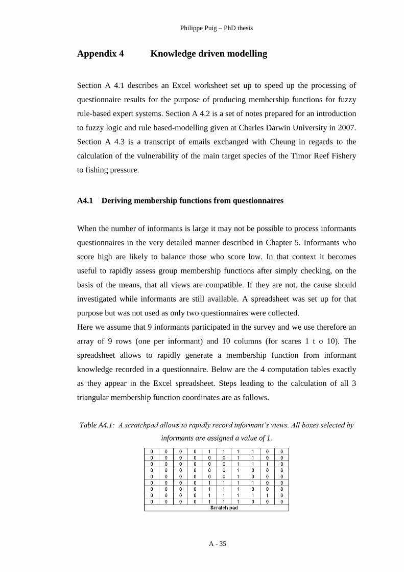
Philippe Puig – PhD thesis
A - 35
Appendix 4 Knowledge driven modelling
Section A 4.1 describes an Excel worksheet set up to speed up the processing of
questionnaire results for the purpose of producing membership functions for fuzzy
rule-based expert systems. Section A 4.2 is a set of notes prepared for an introduction
to fuzzy logic and rule based-modelling given at Charles Darwin University in 2007.
Section A 4.3 is a transcript of emails exchanged with Cheung in regards to the
calculation of the vulnerability of the main target species of the Timor Reef Fishery
to fishing pressure.
A4.1 Deriving membership functions from questionnaires
When the number of informants is large it may not be possible to process informants
questionnaires in the very detailed manner described in Chapter 5. Informants who
score high are likely to balance those who score low. In that context it becomes
useful to rapidly assess group membership functions after simply checking, on the
basis of the means, that all views are compatible. If they are not, the cause should
investigated while informants are still available. A spreadsheet was set up for that
purpose but was not used as only two questionnaires were collected.
Here we assume that 9 informants participated in the survey and we use therefore an
array of 9 rows (one per informant) and 10 columns (for scares 1 t o 10). The
spreadsheet allows to rapidly generate a membership function from informant
knowledge recorded in a questionnaire. Below are the 4 computation tables exactly
as they appear in the Excel spreadsheet. Steps leading to the calculation of all 3
triangular membership function coordinates are as follows.
Table A4.1: A scratchpad allows to rapidly record informant’s views. All boxes selected by
informants are assigned a value of 1.

Philippe Puig – PhD thesis
A - 36
Values in the scratchpad (Table A4.1) are automatically copied in calculation cells of
the array below in Table A4.2 where pre recorded formulas perform two tasks;
it converts each 0/1 answer into the corresponding rank (1 to 10) in the
questionnaire;
it assigns 1000 to columns to be ignored in further calculations and 1 to those
retained.
Table A4.2: A calculation table reads values from the scratchpad in A4.1 and translates
them into scores selected by informants. Scores are tallied for further computations.
Table A4.3: All information in Table A4.1 and A4.2 is summarised to define parameters a, b
and c of the triangular membership function that reflects all informants’ views. Parameter b,
the x coordinate of the apex of the membership function is the average of all selections.
Individual averages in the rightmost column reflect the consistency of all informants’ views.

Philippe Puig – PhD thesis
A - 37
Roles of the Summary Sheet above are to:
reproduce all 0/1 answers recorded by informants;
calculate Average for each informant to rescale answers if necessary;
write minimum and maximum ranks recorded respectively as a and c;
calculate the average of all ranks selected.
Figure A4.1: Triangular membership function automatically derived from
informants’ responses tabulated in Table A4.3.
Figure A4.1 shows the triangular membership function automatically generated by
the points derived from the questionnaire completed by the informants. It
summarises the views of all informants.
A4.2 Introduction to sciFLT, a fuzzy logic toolbox for Scilab
Below is an extract of the material which was presented at a 2 day workshop funded
by the FRDC as part of the project on the development of improved management
strategy for the TRF. The workshop was run at Charles Darwin University on 28 and
29 February 2007 for members of the Darwin marine NRM community. The attached
documents and a CD were given to all attendants. The purpose was to introduce them
to some of the techniques and software used in 2008 to complete FRDC 2005/047
research project funded by the Commonwealth Government.
SciFLT is clearly inspired from FLT, the Fuzzy Logic Toolbox for Matlab. They are
both equally user friendly and can be accessed through commands or through a GUI.
The latter, being more user friendly, is the focus of these notes.

Philippe Puig – PhD thesis
A - 38
SciFLT allows to build and run two types of fuzzy inference systems:
- Mamdani;
- Takagi-Sugeno (T-S).
Only the former type is considered here as it is better suited to the creation of both
knowledge and data driven models while T-S systems are more suited to data driven
models. Mamdani type models tend to be more transparent as well but are not as well
suited to optimization as T-S models.
SciFLT offers many choices of operators and defuzzification techniques:
- the defuzzification technique preferred here is the “centre of gravity”, called
“centroid” in sciFLT and generally considered as the most reliable;
- operators OR and AND can have a number of different mathematical
expressions under the generic names of S-norm and T-norm. Those we
choose here are the default options: algebraic sum and algebraic product.
- the default option complement to one is selected as well;
- the aggregation method however is sum instead of maximum.
Once these options are selected the remaining tasks consists in;
1/ defining/drawing the membership functions of all input and output variables;
2/ writing the rules that make up the fuzzy model;
3/ running the fuzzy model on a set of input values to calculate the output;
4/ visualising the transfer surface which is the 3D surface obtained when all but
two input variables have a set value. This 3D surface allows to observe how
the output, plotted vertically (Z) changes with the two “free” variables plotted
along the X and Y axes.
Owing to time constraints and the lack of prior knowledge of most of the audience
we will go against the chronologic order. Tasks 2 and 1 particularly are more time
consuming and somewhat easier to complete when one has an overview of all steps
involved.
We will use Cheung’s expert system already coded in Scilab to:
- learn how to access the scFLT GUI,
- explore its transfer surface;
- calculate the intrinsic extinction vulnerability of a commercial species given
some its biological characteristics;
- discover the rule editor;
- modify some membership functions.

Philippe Puig – PhD thesis
A - 39
Although a very capable and useful tool, sciFLT 0.2, the latest version available,
completed by Jaime Urzua Grez in 2004 suffers from some limitations. Two were
identified through the implementation of Cheung’s expert system described in
Chapter 6:
the first one relates to flaws in graphic functions resulting in artificially
truncated tips of triangular membership functions clearly noticeable in Figure
6.1 in membership functions M and H of Age_first_mat and Lw and Lw and
M of VBGF_param_K;
the second one less obvious but more troublesome is the inability of sciFLT
to assign weightings to rules. The software allows weightings to be entered
and recorded as displayed in Figure 6.4. Weightings used in all calculations,
however, remain equal to 1.
When Jaime Urzua ([email protected]) was contacted after noticing that
changing weightings had no effect on the output of Cheung’s model. He
confirmed that weighting functionality was planned (the shell had been
created) but not implemented in sciFLT 0.2, the latest version of the software
he released in 2004.

Philippe Puig – PhD thesis
A - 40
1/ Loading the sciFLT functions:
- open the toolboxes pull down menu,
- double click on sciFLT_0.2,
- press ENTER.
21
The sciFLT tool box is now loaded.
22
2/ Open the sciFLT GUI called “sciFLT fls
Editor”
- at the command line type editfls;
- type ENTER;
- the Graphic User Interface (GUI) is now
loaded.
23
3/ Change to the directory where Cheung’s
expert system is saved
C:\TEMP\FRDC_WORKSHOP\SCILAB\
DATASET\Fls_intrinsic_extinction_vulne
rability
use the technique shown in 13
24

Philippe Puig – PhD thesis
A - 41
4/ Open the expert system
- in the sciFLT fls Editor, in the File pull
down menu click
Import
from file
25
5/ Select “Cheung2005_61101.fls”
26
- press Open;
- the truncated name “Cheung_2005” of the
expert system now appears in the sciFLT fls
Editor;
- Cheung’s expert system is now loaded in
Scilab.
27
- press on the blue + in the square
immediarely to the left of the expert system
name;
- details of the expert sys tem appear
type: m
number of inputs: 8
number of outputs: 1
number of rules: 24
28

Philippe Puig – PhD thesis
A - 42
6/ Click on Description
to view a detailed description of the choices
made to build this expert system
29
7/ Click on Inputs
to see the list of Input (independent)
variables
30
8/ To view the coordinates membership
functions and their type
- click on the blue + immediately to the left
of inputs;
- click on the name of the membership
function you want to check, Max_length for
instance.
31
9/ To view the plots of all membership
functions
- click on the View pull down menu;
- click on Plot Current Var.
32

Philippe Puig – PhD thesis
A - 43
Membership of all variables are displayed
33
10/ To display all rules that make up the
expert system
click on Rules
34
11/ To plot the output surface of the fuzzy
logic system
- at the command line type clc to clear the
screen;
- load Cheung expert system and name it
fls;
- call plotsurf to view the output surface of
this fls.
35

Philippe Puig – PhD thesis
A - 44
- press ENTER to access to access the
output surface GUI;
- click the bottom border of the surfplot
window to resize it until you can see all
variables.
36
12/ Enter all following parameters
X axe Nat_mort
Y axe Fecundity
Z axe Vulnerability
Max- Length 71
Age_first_mat 2.5
VBGF_param_K 0.23
Max_age 18
Geo_range 3200
Spat_behav 70
37
13/ Default settings need to be changed
- the default setting of Axes properties
causes the 3D surface to be compressed;
- this setting needs to be changed.
38

Philippe Puig – PhD thesis
A - 45
14/ Edit graphic box properties
in the Scilab Graphic editor where the
compressed 3D surface is displayed, click on
Current Access Properties in the Edit pull
down menu’
39
15/ Edit Axes Properties
check the Cube scaling box
40
The coloured 3D surface provides an easy way
of exploring the effects of fluctuations in
Fecundity and Natural Mortality on the
Vulnerability of the species characterized by:
Max- Length 71
Age_first_mat 2.5
VBGF_param_K 0.23
Max_age 18
Geo_range 3200
Spat_behav 70
41
16/ Find information on sciLab commands
- the sciFLT Help files are not available on
line under Windows (they are under Linux);
- check the syntax of the evalfls and
fscanfMat command respectively from the pdf
sciFLT Help Files and the compiled HTML
Help files (these documents are saved in the
work directory);
- type these commands.
42

Philippe Puig – PhD thesis
A - 46
- loadfls loads the required fuzzy logic system
from the workspace;
- fscanfMat translates rows of input
parameters (initially entered in Excel and
saved as .txt tab delimited text file) into a
matrix of 1 row and 8 columns;
- evalfls saves the value of fls in output.
- read output and M.
43
Although a very capable and useful tool, sciFLT 0.2, the latest version available,
completed by Jaime Urzua Grez in 2004 suffers from some limitations. Two were
identified through the implementation of Cheung’s expert system described in
Chapter 6:
the first one relates to flaws in graphic functions resulting in artificially
truncated tips of triangular membership functions clearly noticeable in Figure
6.1 in membership functions M and H of Age_first_mat and Lw and Lw and
M of VBGF_param_K;
the second one less obvious but more troublesome is the inability of sciFLT
to assign weightings to rules. The software allows weightings to be entered
and recorded as displayed in Figure 6.4. Weightings used in all calculations,
however, remain equal to 1.

Philippe Puig – PhD thesis
A - 47
A4.3 William Cheung’s comments
Below is an exchange of emails with William Cheung referring to calculations of the
vulnerability of the Gold band snapper (Pristipomoides multidens) to fishing pressure.
Dear Philippe,
I estimated the intrinsic vulnerability index for Pristipomoides multidens based on
the parameters that you provided. My estimate is very close to yours, although
slightly lower 60.2. I wonder whether the difference is because of some differences in
the implementation of the fuzzification/defuzzification process somewhere between
the two. But it is good that we have consistent estimates.
Based on the information from fishbase, P. multidens is described as a schooling fish.
Based on the calculation noted in the Cheung et al 2005 paper, a schooling fish will
get a score of spatial behaviour strength (measure of the tendency/frequency) to form
aggregations) of 80. When I included this in the calculation, the predicted intrinsic
vulnerability increased to 66.9. The rationale behind this rule is that it is generally
agree that species that from aggregations, particularly those that are predictable
(e.g. schooling, spawning aggregation) will be more vulnerable to exploitation
because 1. it can be easily targeted, 2. catch-per-unit-effort would like to remain
stable under stock decline because dense schools may continue to form by range
contraction or situation of actual fishing time from targeting different aggregation
(similar to a type II predator-prey functional response) leading to hyper depletion,
i.e. catch-per-unit-effort remains high even stock abundance level is low, marking
the stock/species prompt to serious depletion, 3. disruption of this aggregation may
like have an impact on the population (e.g. depletion of spawning aggregation may
considerably affects recruitment). Therefore, this attribute is included in the
calculation and in fact, from our analysis, it seems to be an important factor in
ranking the relative intrinsic vulnerability in some cases (e.g. reef fishes).
The geographic range is too wide for this species to trigger any rule to be fired so it
doesn’t matter if this is not included. Also, our analysis and other empirical studies
suggest that this is not an important factor affecting the intrinsic vulnerability of

Philippe Puig – PhD thesis
A - 48
MARINE fishes, unless the geographic range is very small (e.g. endemic only to a
small patch of reefs or around a small island).
I hope the above is useful for your analysis. Again, I am very happy that if this study
can be taken to practical uses. I should be greatly appreciated if you would let me
know how your works go later. Please feel free to let me know if you need further
information from me.
By the way, for your interest, a paper is published applying this method to evaluate
seamount fishes (see attached) and there will be a couple more that hopefully will
come out soon. Also, we have a paper in view using the average intrinsic
vulnerability weighted by the annual catches of assemblages and we show that it can
be a useful indicator to evaluate changes in species composition resulted from
fishing.
Best regards,
William
Member, IUCN Specialist Group of Groupers and Wrasses
Fisheries Centre
Aquatic Ecosystems Research Laboratory (AERL)
2202 Main Mall
The University of British Columbia
Vancouver, BC
Canada V6T 1Z4
tel:+1 (604) 822-2731
fax:+1 (604) 822-8934
From: Puig, Philippe (EWLS) [mailto:[email protected]]
Sent: Monday, November 06, 2006 2:33 PM
To: William Cheung
Subject: Expert system

Philippe Puig – PhD thesis
A - 49
<<Scilab_screencapture_061105.doc>>
Dear William
I found your 2005 paper “A fuzzy logic expert system to estimate the intrinsic
extinction vulnerabilities of marine fishes to fishing” particularly interesting.
I built your expert system in sciFLT, the fuzzy logic toolbox for Scilab, an open
source freeware clone of MATLAB. Screenshots are attached.
Julie Lloyd, senior fishery research scientist from Northern Territory Fisheries and I
are co-investigator in a Commonwealth funded research project. Our aim is to
develop of ecologically based management strategies for the Timor Reef Fishery,
about 200km north of Darwin in Australia.
We believe that your extinction vulnerability ranking of commercial fishes should be
part of a long term management of the Timor Reef Fishery. I tested your model with
the life history parameters for P. multidens, the main target species in that fishery.
Maximum length =71.1 cm
Age at first maturity=5 years
VBGF parameter k=0.23
Natural Mortality rate=0.14
Maximum age= 18 years
Geographic range?
Fecundity=1.65x10⁵ eggs/individual/year
Spatial behaviour?
As I was missing two parameters, I eliminated all corresponding rules from the
expert system. This, according to your tests, should only have a minor impact on the
output of the model.
I found a vulnerability index of 61.4. This puts P. multidens in the same vulnerability
category as the Atlantic cod.
This leads me to two questions:
1/ would you mind checking that you find the same vulnerability index for P.
multidens with your model;

Philippe Puig – PhD thesis
A - 50
2/ I did not include in my model rules 24 and 25 corresponding to attribute 8 on page
101 of your article. I assume that they play the role of edges. Could you please
elaborate on these last two rules.
Thank you very much for a very good article which will hopefully contribute to
giving to fuzzy logic the importance it should have in fishery science.
Regards
Philippe Puig
Senior Spatial Scientist
EWL Sciences
PO Box 39443
Winnellie NT 0821
Australia
Tel: 61 8 8922 5219
Fax: 61 8 8922 5260