The Role of Labor‐Market Changes   In the Slowdown of European Productivity Growth 

   

Ian Dew‐Becker (Harvard University) Robert J. Gordon (Northwestern University, NBER, CEPR) 

  

To Be Presented at NBER Productivity Program Meeting , Cambridge, December 7, 2007 

  

This Version, December 2, 2007       

 * Thanks to Bobby Krenn for superb research assistance, including his authorship of the 

Data Appendix.  We are grateful to Bart van Ark, Susanto Basu, Richard Freeman, Greg Mankiw, Bill Nordhaus, and the Economic Policy editors and referees for their perceptive comments on earlier versions and to Andrea Bassanini, Romain Duval, Magnus Henrekson, and Guido Schwerdt for providing data. 

The Role of Labour‐Market Changes   In the Slowdown of European Productivity Growth 

 Abstract 

 Throughout the postwar era until 1995 labor productivity grew faster in Europe than in the United States.  But since 1995, productivity growth in the EU‐15 has slowed while that in the United States has accelerated.  But Europe’s productivity growth slowdown was largely offset by faster growth in employment per capita, leaving little difference in growth of output per capita between the EU and US going back to 1980.  This paper is about the strong negative tradeoff between productivity and employment growth.  We document this tradeoff in the raw data, in regressions that control for the two‐way causation between productivity and employment growth, and we show that there is a robust negative correlation between productivity and employment growth across countries and time.  We simplify the task of explaining intra‐EU differences in the performance by reducing the dimensionality of the issue from the 15 EU countries to four EU country groups, chosen by geography.  We provide a comprehensive analysis of the role of policy and institutional variables in causing changes in productivity and employment per capita growth across these country groups.  Using both a calibrated theoretical model and several reduced‐form regressions, we document the strong effects of European policies that raised labour costs, such as the tax wedge, employment and product market regulation, unemployment compensation, and union density, in causing employment to fall and productivity to rise before 1995, and for this process to be reversed after 1995.    Our paper concludes with policy implications, and we propose a new framework for thinking about EU policy reforms.  The strong evidence that we find for a productivity‐employment growth tradeoff changes the questions that European policymakers should be asking.  They should no longer ask how they should boost productivity growth or raise employment growth.  Most policies will push productivity and employment in opposite directions, and we have shown that these offsetting effects make the effects of policies on growth in output per capita ambiguous.  Our new policy framework suggests that policy changes be assessed as much on their effects on government budgets as on productivity or employment, since the productivity‐employment tradeoff causes some policy changes to have a negligible effect on growth in output per capita.  Ian Dew‐Becker                                                                                                               Robert J. Gordon Department of Economics                                                                              Department of Economics Harvard University                                                                                          Northwestern University Cambridge MA 02138                                                                                         Evanston IL 60208‐2600 idew@fas.harvard.edu                                                                                            rjg@northwestern.edu 

1

1. INTRODUCTION  

Throughout the postwar era until 1995 labor productivity grew faster in Europe than in the United States.  But since 1995, productivity growth in the EU‐15 has slowed while that in the United States has accelerated.  What caused this reversal?  In principle one could imagine any number of causes, including a spontaneous acceleration in total‐factor productivity (TFP) growth in the U.S., a spontaneous deceleration of TFP growth in Europe, a change in labor‐market policies and institutions in Europe that made labor both cheaper and less productive, a change in the level of investment in Europe, or any combination of these.   

 The starting point for the paper is the observation that after 1995, just as Europe’s 

labor productivity growth slowed down relative to the US, its growth in hours worked per capita surged relative to the US.  Moreover, the countries within Europe that had the largest decelerations in productivity growth also had the largest increases in hours.  As a result, the growth of European output per capita has fallen behind that of the US by a much smaller margin than its shortfall in the growth of labor productivity.  Are the simultaneous turnarounds of productivity and hours per capita in opposite directions independent or related events, and if related in which direction does the causation run and what were the underlying causes?   

 While we begin with contrasts between the US and EU‐15, most of this paper is 

about heterogeneity within the EU‐15.  To facilitate generalizations about heterogeneity within Europe, we group European countries into the same geographical sub‐aggregates as in Boeri et al. (2005), namely the Nordic, Anglo‐Saxon, Continental, and Mediterranean countries. 1  We pay particular attention to the contrast between the Mediterranean group and the other three groups, because the slowdown in productivity growth and revival of growth in hours per capita has been particularly pronounced in the two biggest Mediterranean countries, Italy and Spain.  We also highlight the relatively strong performance of the Nordic and Anglo‐Saxon country groups in both productivity and employment growth.  The average population shares of the four groups over 1980‐2004 were 5 percent for the Nordic group, 17 percent for the Anglo‐Saxon group, 49 percent for the Continental group, and 29 percent for the Mediterranean group.  

 An initial decomposition shows that Europe’s turnaround in hours per capita has 

occurred not in hours per employee but rather primarily in employment per capita.  We explore as carefully as possible the post‐1995 turnaround in the growth of European employment per capita from negative to positive in most countries and to very rapid in 

1The only difference is that we label their “Other Europe” group as “Continental” and we group Ireland with the UK in the “Anglo‐Saxon” group rather than in the “Other Europe” group as they do. 

some countries.  A large literature has examined the dimensions of policy and institutions which in Europe made labor more expensive before 1995; this literature examines the effects of, among other things, labor tax wedges, labour‐market and product‐market regulations, union density, and unemployment compensation.  

 Our first empirical task is to describe the behavior of the leading policy and 

institutional variables that have been identified as relevant in the past literature on the pre‐1995 decline in European hours per capita relative to the US.  Our list of policy and institutional variables includes four policy variables – the labor tax wedge, the average replacement rate of unemployment insurance, and indices of employment protection legislation and  product market regulation.  Also included are two institutional variables describing outcomes rather than policies themselves, trade union density and an index of “corporatism.” 

 We examine changes in these policy/institutional variables over the time period 

between 1978 and 2003.  Some of the variables, particularly the time wedge, display a post‐1995 turnaround (from rising to falling tax rates) that is perfectly timed to help explain the turnaround in employment and productivity growth.  Other variables turn around much earlier or do not turn around at all.  Thus our initial exploration of the time path of the policy/institutional variables provides some caution and qualification to the easy verdict that everything—policy, institutions, and outcomes – all turned around simultaneously after 1995. 

 Next we ask is whether there is any systematic relationship between these 

sources of higher pre‐1995 labour costs and the subsequent post‐1995 upsurge in European employment per capita.  Before 1995, Europe could have been described as making labour more expensive through taxes and regulation, driving its labour market northwest along the labor demand curve.  In this northwest movement we naturally observe both a decline in employment and also an increase in productivity as some employees lose their jobs due to changes in policies and institutions that make it more expensive for employers to hire labour.   

 Starting at different dates for different policies, Europe has begun the process of 

deregulation, encouraging higher employment per capita, which we find both fostered the increased employment of less experienced employees and lowered the capital intensity of the economy.  Our analysis finds that Europe shifted to the southeast along its labour demand curve, toward higher employment per capita but lower average productivity per hour.   

 It is clear from the outset that our results need to be highly qualified.  Policy and 

institutional variables turned around at various dates, not all in 1995 but over a span of time from 1982 to 2001.  Policy and institutional variables do not explain all or even most of the post‐1995 upsurge in European employment per capita.  Much of the post‐1995 

2

employment increase has occurred for females, not males, and we interpret this not as a result of specific policy interventions but rather as a shift in culture and social norms toward a greater acceptance of females in the labor force, especially in Southern Europe.    

We distill a large European literature on the adverse effects of policies and institutions in dampening European employment per capita and raising labor productivity before 1995.  We ask to what extent these policies and institutions were reversed after 1995 and to what extent this policy turnaround explains the employment and productivity growth turnaround that followed.2  We develop regression models building on some of the best recent research to identify which policies and institutions changed and how much of the employment turnaround can be explained by these models.  The size of our dataset – 23 years of data for 15 countries – gives us substantial power for identifying the relevant effects.  Our paper is also unique in developing post‐1995 simulations that quantify the ffect of the policy and institutional variables.  Even some of the most recent papers in this literature, e.g., Ohanian, Raffo, and Rogerson (2007), carry out an analysis that focuses on pre‐1995 relationships without any attempt to test their pre‐1995 hypotheses on post‐1995 data. 

 The paper then proceeds to the relationship between employment and 

productivity using two methods.  The first is to develop a simple structural model based on the neoclassical growth model and augment it to account for variation in experience and talent across the population.  This allows us to trace the effects of female and male employment growth and to quantify how employment growth should affect not only productivity, but also investment and total output.  While the model is necessarily extremely simple, it explains a surprisingly large part of the variation in productivity across Europe.  By applying this model to the four country groups, we also identify an unexplained decline in the growth of capital investment as part of the Mediterranean productivity problem, as well as an unexplained increase in the growth of investment in the Continental and especially in the Nordic countries. 

 Second, we develop an explicit econometric model that attempts to explain 

changes in labour productivity growth as a function of the turnaround in employment per capita.  This model uses standard statistical procedures to eliminate the feedback from productivity growth to employment growth and allows us to measure the feedback from policy changes such as the reduction in the European tax wedge as a factor explaining higher employment growth and slower productivity growth after 1995.   

 The productivity regressions are not designed to maximize R2.  We do not 

explain the majority of the post‐1995 productivity turnaround in Europe, and there is no evidence that the entire slowdown was driven by the increase in employment.  Rather, 

2 Two important books on the European reform agenda are Baily and Kirkegaard (2004) and Alesina and Giavazzi (2006). 

3

our focus is on identifying as precisely as possible the magnitude of the effects of employment and government policy on employment.  We find that there is a strong and robust negative correlation between productivity growth and employment per capita across Europe.  Moreover, two of the policy variables (the replacement rate of unemployment benefits and an index of employment protection legislation) have significant direct positive effects on productivity growth in addition to their indirect effects through employment.  Last, we study the complete effects of policy changes on productivity, employment, and output per capita.  

 Our story of declining European productivity growth emerges with multiple 

dimensions, including the impetus from changes in policies and institutions, and from other possible independent causes of employment growth, particularly in the Mediterranean countries.  

 Our paper concludes with policy implications.  We find that changes in some of 

the policy and institutional variables that we examine have opposite effects on employment and productivity growth.  We suggest that the policy dialogue take this tradeoff into account and examine the net effect of the opposing impacts on employment and productivity, that is, by looking at the net effect of such changes on the growth rate of income per capita.  We examine statistical confidence bands to ask whether given changes in policy and institutional variables create a significant positive, significant negative, or insignificant effect on the growth rate of per‐capita income in Europe after 1995.    

2. DATA ON THE TWIN TURNAROUNDS 2.1 The Opposite Movements of Growth in Labour Productivity and Hours per Capita

   The story of the joint post‐1995 turnaround in productivity and hours per capita is best told in Figure 1.  Figure 1 plots our three core variables, labour productivity or output per hour (Y/H), versus hours per capita (H/N), and their product (output per capita, or Y/N), in a form that smooths the annual year‐to‐year wiggles of the data into long‐run trends.3  We express hours and output on a per‐capita basis, which partly levels the playing field due to the 0.7 percent per annum slower rate of population growth in the EU than in the US.4  3 The trends are created by a Hodrick‐Prescott filter applied to annual data with a smoothing parameter of 12.5.   The US trends are based on taking the annual average of trends fitted to quarterly data through 2007Q2, in order to highlight the 2004‐06 downturn in US productivity growth.  4 The difference between EU‐15 and US popution growth differs by concept and data source.  With GGDC data EU‐15 growth in total population grew 0.7 percent slower than in the US over 

4

 The upper frame of Figure 1 exhibits the growth trends of EU and US output per 

hour since 1970 in the total economy (not the more frequently cited private business sector).  The EU growth trend uniformly falls from about 5 to 1 percent per year, with a brief hiatus in the decline between 1988 and 1996.  The US growth trend declined in the 1970s to a trough in 1981, then exhibited a modest recovery in the early 1980s and a much more significant revival after 1996.  The difference between the EU and US growth trends changed from +2.2 percentage points in 1970 to ‐0.6 percentage points in 2006. 

 The bottom frame of Figure 1 expresses growth in both output and hours per 

capita.  The graph shows that the US trend growth in hours per capita was positive in most years until 2000, but negative from 2000 to 2005.  In contrast, trend growth in Europe’s hours per capita was strongly negative from 1970 to 1995, with a brief interruption in 1986‐89.  This negative trend reversed itself over the past decade, recording a positive trend growth rate of hours per capita in each year after 1995.   

 When Y/H is multiplied by H/N, the divergent trend growth rates of 

productivity and hours per capita imply a surprisingly small EU‐US difference in the growth rate of output per capita (Y/N).  While Europe did show faster growth in the early 1970s, since then there has been a tie game, with average trend growth rates over 1975‐2006 of 1.92 percent per year for the EU and 1.97 percent for the US.  The problem is that Europe has failed to catch up to the US level of output per capita since 1975.  Its achievement of maintaining roughly similar growth rates to the US since 1975 has left the EU‐US ratio of output per capita roughly fixed at around 70 percent of the US level.  

 Growth of hours per capita is equal by definition to the growth of hours per 

employee (H/E) plus the growth of employees per capita (E/N).  We choose in this paper to focus our analysis on the European turnaround in employment per capita.  As shown in Figure 2, the post‐1995 turnaround in employment per capita is much more dramatic than in hours per capita.  For the rest of this paper, we will use the metric of employment per capita to summarize the European post‐1995 turnaround, and we will subsequently disaggregate the overall change in employment per capita by looking at its components by age and sex. 

 Figure 1 raises an important question relevant to the interpretation of this paper.  

We are intrigued by the joint turnaround in opposite directions after 1995 between the US and EU‐15 in the growth rates of employment per capita and in labor productivity.  But clearly this turnaround‐tradeoff story is not adequate to characterize the entire post‐1970 period plotted in Figure 1, where in the top frame the growth of labor productivity slowed much more between 1970 and 1980 and with no apparent corollary of rapid 

1970‐2006.  With OECD data the difference for total population was 0.54 percent and for population aged 15 and over was 0.53 percent.

5

growth in hours or employment per capita.  We view the story of declining productivity growth in the 1970s in both the US and EU‐15 as outside of the scope of this paper.  The focus and regression analysis of this paper concentrates on the turnaround in the behavior of both productivity and employment growth between the periods 1980‐95 and 1995 until 2003.  

 2.2 The Turnaround by Country and EU Country Group

 Table 1 summarizes the 1970‐95 and 1995‐2006 growth rates of Y/H, H/N, and Y/N 

for the US, the EU‐15, each EU country, our four EU country groups, and for the EU‐15 excluding the Mediterranean countries.  We focus here primarily on the turnarounds, that is, the difference between the 1995‐2006 and 1970‐95 growth rates for each of the three variables.  The EU‐US turnaround difference is ‐2.20 percentage points for Y/H, +1.99 points for H/N, and a mere ‐0.19 points for Y/N.  These numbers are not listed explicitly in Table 1; they are calculated by taking the EU line and subtracting the US line in the column labeled “difference.” 

 The role of the Mediterranean countries is shown by a separate “EU‐15xMed” 

aggregate that excludes the three Mediterranean countries.  The negative Y/H turnaround when the EUxMed countries are compared with the row for the US becomes smaller from ‐2.20 points to ‐1.65, the H/N turnaround becomes smaller from +1.99 to +1.50 points, and the Y/N turnaround becomes smaller from ‐0.19 to ‐0.15 points.  Thus, while the Mediterranean countries contribute disproportionately to the post‐1995 turnarounds in Y/H and H/N, still a substantial turnaround in both productivity and employment growth remains in the rest of the EU‐15.     An important development in Europe since 1995 has been an increase in heterogeneity across countries.  The bottom line in Table 1 shows that there has been an increase in the standard deviation across EU countries of all three variables, with a doubling in the standard deviation for H/N and Y/N.  With only a few exceptions, pre‐1995 growth in Y/N was in the range of two to three percent, but after 1995 the range was from a low of 1.18 percent for Italy to a high of 6.17 percent for Ireland.      The large negative tradeoff between Y/H and H/N growth in Spain leaves that country with an impressive post‐1995 growth performance in Y/N.  Two of the Mediterranean countries, Greece and Spain, are ranked number two and three among the EU‐15 in post‐1995 Y/N growth, exceeded only by the outstanding performance of Ireland.  The Y/N growth outcome also points to the sharp contrast between Spain and Italy; both Italy and Spain had near‐zero productivity growth after 1995, but Spain had a much more impressive growth rate of H/N, thus leading to a growth rate of Y/N in Spain almost triple that in Italy.     

6

2.3 Labour and Capital Ratios and Total Factor Productivity    We now bring together data on countries including the US, the EU, and the four EU country groups, and compare the turnaround in Y/H and E/N with other components of growth accounting, namely the growth of hours per employee (H/E), in capital input per hour (K/H), capital deepening (the income share of capital times growth in K/H), and growth in total factor productivity (TFP).  The numbers on the Y/H and E/N post‐1995 turnarounds are slightly different in Figure 3 and Table 2, which applies to 1980‐2004, than in Table 1 that covers the longer period 1970‐2006.  This difference in dates is due to data availability regarding capital and TFP.  

Figure 3 examines data on the trend growth rate in capital per hour (K/H) and in total factor productivity (TFP).  Taking account of the differing time periods in Figures 3 and Figure 1, the time path of EU growth in K/H roughly parallels that of Y/H, with respective 1980‐2004 decelerations between 5 and 2 percent annual growth for K/H versus between 3 and 1 percent annual growth for Y/H.  In the US the growth rate of K/H showed both a greater 1980‐95 growth slowdown than Y/H and also a somewhat larger post‐1995 growth bulge than in Y/H.  These differing patterns cancelled out for K/H, with exactly the same 1980‐95 and 1995‐2004 growth rates for the US as shown in Table 2.   

 As shown in the bottom frame of Figure 3, the growth rate of TFP slowed 

steadily in the EU from 1983 to 2004 while that in the US accelerated in stages.  The difference in TFP growth between the EU and US may be exaggerated by data discrepancies. 5      We find several interesting facts in the bottom section of Table 2.  For the US the turnarounds of Y/H and TFP were identical and there was no turnaround in the capital deepening effect.  This occurred as the result of slowdowns in the growth of capital per capita and hours per capita by the same amount, ‐0.49 percent.  In the EU as a whole, the capital growth turnaround was about the same as the output growth turnaround, as shown by the small positive turnaround in the K/Y ratio at the bottom of the table.  This implies that the negative turnaround in K/H growth was almost as large as the positive turnaround in H/N growth.  As a result of this turnaround in the capital‐deepening effect, the turnaround of TFP growth was ‐0.80 percentage points, slightly less than the ‐0.93 turnaround of Y/H growth.    

The four country groups display interesting differences.  To what extent was growth in capital stimulated by growth in employment?  An easy way to obtain this 

5 Standard growth accounting data for the US from US sources obtained from Kevin Stiroh suggests much slower K/H growth and much faster TFP growth in the 1980s than implied by the EU‐KLEMS data displayed in Figure 3. 

7

information from Table 2 is to compare the turnaround in capital per capita growth with that in employment per capita growth.  The Nordic group had a modest negative turnaround in Y/H growth and hardly any negative turnaround in TFP growth.  This difference by definition is due to the fact that the negative turnaround in capital deepening was nearly twice as large as the TFP turnaround and thus accounts for most of the Y/H turnaround.  The negative turnaround in the K/H ratio was entirely due to the increase in H/N, as the K/N turnaround was close to zero.  Thus our main impression is that the Nordic countries had a disappointing performance of investment despite a large turnaround in employment and a relatively strong productivity performance. 

 The Anglo‐Saxon group is mainly driven by the UK.  This group had the smallest 

Y/H turnaround of the four European groups by a narrow margin, and the second‐smallest TFP turnaround.  The slowdown in K/H was much smaller than the increase in hours, due to a substantial increase in the growth rate of K/N.  The Anglo‐Saxon group thus has the best performance overall, with a modest slowdown in labour productivity and growth in capital per capita that was almost half the turnaround in employment per capita.   

 Not surprisingly, with its 49 percent population share in the EU‐15, the 

performance of the Continental group was similar to the EU as a whole.  The decline in both Y/H and TFP growth was similar to the EU, while the sluggish revival of growth in E/N was partly compensated for by an atypical turnaround toward positive growth in H/E.  The slowdown in the capital deepening effect was dampened both by a modest increase in growth of K/N and a small increase in the income share of capital.  The modest positive turnaround in capital per capita growth was roughly one‐third of the size of the turnaround in employment per capita growth.   

 As we have already seen, the Mediterranean group had the most noteworthy 

turnarounds for Y/H, E/N, K/H, capital deepening, and TFP.  The slowdown in Mediterranean capital deepening was relatively modest, because the sharp negative turnaround in K/H growth was partially offset by a sizeable increase in the income share of capital (from 28 to 34 percent).  We note that the negative turnaround in K/H growth was entirely due to faster growth in E/N, and that the turnaround in capital per capita growth was less than one‐tenth of the turnaround in employment per capita.  Thus a surprising finding is that the Mediterranean countries shared with the Nordic countries a disappointing performance of capital growth, while both the Anglo‐Saxon and Continental groups display a positive response of capital per capita to more rapid growth in employment per capita. 

 Simple growth accounting, however, does not allow us to determine whether 

there was a negative investment shock in the Nordic and Mediterranean countries.  Shocks have to be determined based on some baseline.  In section 6, we will explicitly 

8

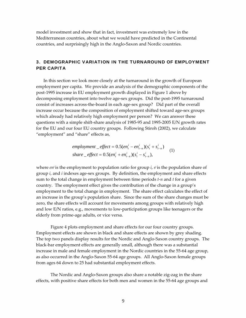
model investment and show that in fact, investment was extremely low in the Mediterranean countries, about what we would have predicted in the Continental countries, and surprisingly high in the Anglo‐Saxon and Nordic countries.   3. DEMOGRAPHIC VARIATION IN THE TURNAROUND OF EMPLOYMENT PER CAPITA

In this section we look more closely at the turnaround in the growth of European employment per capita.  We provide an analysis of the demographic components of the post‐1995 increase in EU employment growth displayed in Figure 1 above by decomposing employment into twelve age‐sex groups.  Did the post‐1995 turnaround consist of increases across‐the‐board in each age‐sex group?   Did part of the overall increase occur because the composition of employment shifted toward age‐sex groups which already had relatively high employment per person?  We can answer these questions with a simple shift‐share analysis of 1985‐95 and 1995‐2005 E/N growth rates for the EU and our four EU country groups.  Following Stiroh (2002), we calculate “employment” and “share” effects as, 

 

),)((5.0_

))((5.0_i

ntit

int

it

int

it

int

it

sseneneffectshare

sseneneffectemployment

−−

−−

−+=

+−=    (1) 

 where eni is the employment to population ratio for group i, si is the population share of group i, and i indexes age‐sex groups.  By definition, the employment and share effects sum to the total change in employment between time periods t‐n and t for a given country.  The employment effect gives the contribution of the change in a group’s employment to the total change in employment.  The share effect calculates the effect of an increase in the group’s population share.  Since the sum of the share changes must be zero, the share effects will account for movements among groups with relatively high and low E/N ratios, e.g., movements to low‐participation groups like teenagers or the elderly from prime‐age adults, or vice versa.    Figure 4 plots employment and share effects for our four country groups.  Employment effects are shown in black and share effects are shown by grey shading.  The top two panels display results for the Nordic and Anglo‐Saxon country groups.  The black‐bar employment effects are generally small, although there was a substantial increase in male and female employment in the Nordic countries in the 55‐64 age group, as also occurred in the Anglo‐Saxon 55‐64 age groups.  All Anglo‐Saxon female groups from ages 64 down to 25 had substantial employment effects.   

The Nordic and Anglo‐Saxon groups also share a notable zig‐zag in the share effects, with positive share effects for both men and women in the 55‐64 age groups and 

9

negative share effects in the 25‐34 age groups.  This suggests that employment shares shifted toward relatively old prime‐age workers with high employment rates and away from relatively young workers with low employment rates.  This is likely the result of the aging of the population.  It turns out that the share effects all cancel out, and their sum is only ‐0.01.  Intuitively, this is because the groups across which the population has been shifting all have similar employment rates.6    The bottom left quadrant of Figure 4 shows that, if anything, employment effects in the Continental countries were less important than in the Nordic and Anglo‐Saxon countries.  But there were substantial share effects, particularly for the 25‐34 age group where employment fell drastically for both males and females.    The bottom right panel of figure 4 plots data for the Mediterranean countries.  Again, there is the same effect of aging on the share effects, but the employment effects are substantially larger.  91 percent of the 6.6 percentage point increase in the employment rate in the Mediterranean countries is explained by employment effects, and the remainder by share effects.  Since women started the period with much lower employment than men, we would expect most of the increase to be concentrated among women.  As it turns out, 70 percent of the total Mediterranean employment increase can be explained by employment effects for women.  Moreover, this increase is not just concentrated among the young; it is spread across all age groups except 65+, and is focused on the prime working years.    The pattern of female employment explaining employment changes extends across three of our four country groups.  In addition to the Mediterranean countries, female employment effects explain 68 and 59 percent of the total employment increases in the Nordic and Anglo‐Saxon countries, respectively.  In the Continental countries, female employment contributed a 1.3 percent increase in aggregate employment, but share effects and male employment canceled out essentially all of that.  In the end, Figure 5 summarizes two important findings of this paper.  First, we confirm the result that the European work force is aging, but aging has not yet substantially reduced employment.    

The second result is that the majority of employment changes in Europe following 1995 can be explained by increases in prime‐age female employment.  There are obviously innumerable policy variables that affect employment.  The shift‐share analysis above helps us narrow down which variables are likely to be the most 

6 There is no reason that share effects actually have to sum to near zero.  For example, if a country’s employment rates by age stayed constant but the country all of a sudden went from being composed mainly of prime age workers to mainly retirees, the associated decline in employment would be entirely explained by share effects. 

10

important, and these are the variables affecting women in their prime working years.7  The distinctly different behavior of the female from the male employment ratios in Figure 4 leads us now to develop regression equations explaining E/N that distinguish between men and women.   4. THE TIME SERIES BEHAVIOR OF THE POLICY AND INSTITUTIONAL VARIABLES  

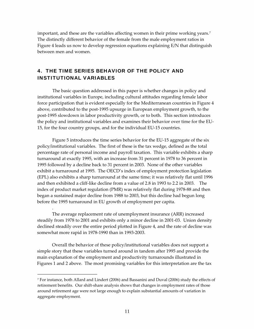
The basic question addressed in this paper is whether changes in policy and institutional variables in Europe, including cultural attitudes regarding female labor force participation that is evident especially for the Mediterranean countries in Figure 4 above, contributed to the post‐1995 upsurge in European employment growth, to the post‐1995 slowdown in labor productivity growth, or to both.  This section introduces the policy and institutional variables and examines their behavior over time for the EU‐15, for the four country groups, and for the individual EU‐15 countries.   

 Figure 5 introduces the time series behavior for the EU‐15 aggregate of the six 

policy/institutional variables.  The first of these is the tax wedge, defined as the total percentage rate of personal income and payroll taxation.  This variable exhibits a sharp turnaround at exactly 1995, with an increase from 31 percent in 1978 to 36 percent in 1995 followed by a decline back to 31 percent in 2003.  None of the other variables exhibit a turnaround at 1995.  The OECD’s index of employment protection legislation (EPL) also exhibits a sharp turnaround at the same time; it was relatively flat until 1996 and then exhibited a cliff‐like decline from a value of 2.8 in 1993 to 2.2 in 2003.    The index of product market regulation (PMR) was relatively flat during 1978‐88 and then began a sustained major decline from 1988 to 2003, but this decline had begun long before the 1995 turnaround in EU growth of employment per capita. 

. The average replacement rate of unemployment insurance (ARR) increased 

steadily from 1978 to 2001 and exhibits only a minor decline in 2001‐03.  Union density declined steadily over the entire period plotted in Figure 4, and the rate of decline was somewhat more rapid in 1978‐1990 than in 1993‐2003.   

 Overall the behavior of these policy/institutional variables does not support a 

simple story that these variables turned around in tandem after 1995 and provide the main explanation of the employment and productivity turnarounds illustrated in Figures 1 and 2 above.  The most promising variables for this interpretation are the tax 

7 For instance, both Allard and Lindert (2006) and Bassanini and Duval (2006) study the effects of retirement benefits.  Our shift‐share analysis shows that changes in employment rates of those around retirement age were not large enough to explain substantial amounts of variation in aggregate employment. 

11

wedge, EPL, and to a lesser extent PMR.  Nevertheless, our regressions attempting to explain the behavior of growth in employment per capita and in labor productivity are based on data for individual countries over time, not just the EU averages plotted in Figure 4.  Which are the countries that had noticeable turnarounds in the policy variables after 1995?   

 Table 3 lists the values of the five policy variables in 1978, 1995, and 2003 for the 

EU‐15 aggregate, the four country groups, and the individual countries.  The tax wedge had a clear turnaround for the EU‐15.  There was a modest turnaround in the tax wedge, in the sense of a decline after 1995, in Finland and Sweden.  A disproportionate share of the tax wedge turnaround was contributed by the Anglo‐Saxon group, including both Ireland and the UK.   

 The tax wedge rose from 1978‐95 in the Continental group and declined only 

modestly during 1995‐2003.  But the Mediterranean countries deliver a substantial turnaround in the tax wedge, following a 5.1 percentage point increase in 1978‐95 with a ‐6.3 percent change in 1995‐2003.   

 The EPL index for the EU‐15 did not increase appreciably between 1978 and 1995 

but did decrease substantially following 1995.  This decline occurred primarily in the Continental and Mediterranean countries, with little change in the Nordic countries and a positive change (from low levels) in the Anglo‐Saxon countries.   

 As is evident in Figure 4, the replacement rate of unemployment insurance 

(ARR) did not decline after 1995 for the EU‐15, but rather its rate of increase slowed.  This increase occurred for most of the EU‐15 population, that is, in the Continental and Mediterranean countries, that offset a sharp reduction in ARR in the Nordic countries and a negligible decrease in the Anglo‐Saxon group. 

 The most dramatic decline in the policy/institutional variables occurred in the 

product‐market regulation index (PMR).  The decline in PMR over the entire period 1978‐2003 was pervasive and appears uniformly in all four of the country groups.  For the Continental and Mediterranean groups, the annual rate of change of the PMR variables was substantially faster after 1995 than before 1995. 

 Finally, union density declines uniformly over the entire period and does not 

offer a promising candidate for the post‐1995 turnaround in employment per capita and productivity.  For the EU‐15 aggregate, union density declined faster before 1995 than after 1995.  Only for the Nordic countries was there a turnaround from increasing union density to declining union density.  In the other country groups the decline in union density was either faster before 1995 or at roughly the same annual rate before and after 1995.   

12

 5. THE RESPONSE OF EMPLOYMENT PER CAPITA TO POLICY AND INSTITUTIONAL CHANGES

The point of departure for our study of the EU employment turnaround is a substantial literature that debates the sources of the postwar decline in the ratio of EU to US hours per capita – 48 percent (in logs) from 1960 to 1995.  There is widespread agreement that Europe made labor more expensive, at least before 1995, but less on the ultimate causes – taxes, regulations, politics, unions, or a mix of these.  On the other hand, there is much less work on understanding how much of the post‐1995 turnaround in H/N can be linked to a reversal of the underlying policy and institutional variables that are often cited as driving pre‐1995 changes.  The primary goal of this section is to advance the literature by documenting the link between the post‐1995 turnaround in the behavior of employment per capita (E/N) and the post‐1995 changes in the policy and institutional variables.  

 5.1 The Previous Literature on Changes in Hours per Capita and Employment per Capita

 As stated above, our study of the European turnaround in labor input growth 

centers on the increased growth of employment per capita rather than hours per capita or hours per employee.  The previous literature includes papers on both hours per capita and employment per capita; we discuss here treatments of both alternatives.   

Prescott (1994) is the best‐known advocate of the view that the sharp decline in European hours per capita is entirely due to high labor taxes.  By “taxes” he means a change in the tax rate or tax “wedge,” broadly interpreted as the sum of the income tax rate and the rate of taxes on labor income paid by employees and employers (what Americans call the “payroll tax rate”).  Prescott establishes his result with theory and calibration methods, and a paper that interprets his results by Alesina, Glaeser, and Sacerdote (2006) calculates that Prescott’s elasticity of hours per capita to a change in the tax wedge is ‐0.92.  That is, an increase in the tax rate t  by one percent reduces hours per capita by 0.92 percent.  The Alesina paper compares Prescott’s methods with a review of the microeconomic labor‐supply literature and concludes that Prescott’s estimates of the tax exaggerate the effect by a factor of two, because tax effects are primarily limited to secondary workers, i.e., females and teenagers.  Thus the Alesina paper argues that the tax elasticity may be only as high as ‐0.40 to ‐0.45. 

  Several papers, including Davis and Henrekson (2004), attempt to replace the assumed tax elasticity of Prescott with elasticities estimated from the data.  These authors use two different time series on tax rates to estimate the elasticity of H/E, H/N, and E/N to changes in the tax wedge.  Here we focus on their results for employment 

13

per capita.  Their paper, like others in the field, adds additional control variables beyond the tax wedge as possible explanations of the pre‐1995 decline in European E/N.   

  The key Davis and Henrekson results are presented in their Table 4 (2004, p. 58).  The tax rate elasticity in E/N regressions is a highly significant ‐0.22 with country fixed effects.  Unlike our results based on annual data for 1980‐2003 as presented below, their evidence is based on only four years (1977, 1983, 1990, 1995).  Similar to the some other papers in this literature, Davis and Henrekson do not present evidence extending past 1995 and thus miss Europe’s post‐1995 turnaround in employment per capita.   

  A paper closely related to ours is that by Allard and Lindert (2006).  Their aim is to sort through all of the exogenous policy variables that might have reduced European hours and employment, but, surprisingly, they do not notice the post‐1995 turnaround in hours or in employment per capita.  The list of policy changes analyzed by Allard‐Lindert is wide‐ranging.    But in the end the Allard‐Lindert analysis is uni‐dimensional.  They pluck candidates to explain lower European hours growth or productivity growth, with no recognition that there may be a negative tradeoff between them.  They also fail to recognize that there may be a two‐way causation between productivity and employment changes. 8   

5.2 Regression Equations Explaining Employment per Capita 

 The most recent and convincing paper in this literature is from Bassanini and 

Duval of the OECD (2006), hereafter B‐D, who explain movements in the unemployment rate and per‐capita employment in a variety of econometric specifications.  We incorporate most of their approach and, using their data developed at the OECD, we provide a somewhat different set of regression equations that are used both to obtain coefficients on the effects of alternative policy and institutional variables, and also to use the estimated coefficients to examine the marginal effect of policy and institutional changes on employment per capita after 1995.  Did the post‐1995 upsurge in employment per capita respond to tax cuts, the decline in union density, or to other variables, and, if so, what were their respective contributions?    

Since we are asking different questions than B‐D, we use a somewhat different specification than theirs.  Whereas B‐D studied the determinants of changes in employment per capita in 20 OECD countries, including the US, Canada, and Japan, our focus is on the EU‐15 minus Luxembourg.  We also weight our regressions by population in order to provide the most appropriate results for discussing the EU, in contrast to their unweighted regressions that give the same importance to Luxembourg 

8 Among other previous sources estimating regressions to explain changes in European labour input are Beaudry and Collard (2001), Blanchard and Wolfers (2000), and Pissarides et al. (2005).  Ljungqvist and Sargent (2006) have joined the debate with Prescott by emphasizing the disincentive role of the welfare state that is paid for by the tax wedge.  

14

and the United States.  The larger countries better represent the EU as a whole and should be treated as such in the regressions.9  Furthermore, in the interest of obtaining results that apply at the aggregate level, we run regressions using the total employment rate, not just broken down by age and gender.    

Last, we run the regressions in growth rates, rather than levels, because we have found that the residuals in the levels regressions seem to follow a random walk.10  Our basic model posits that the level of employment is driven by the levels of the policy variables and the output gap.  We then take the first difference of the entire equation so that the actual regression is of the growth rate of the employment rate (E/N) on the growth rates of the policy variables and the change in the output gap.11 

 In addition to the important change from levels to logarithmic growth rates, 

there are several other technical details in our regressions that differ from B‐D and make them more appropriate for the questions that we ask in this paper.  Our baseline results differ from those of B‐D by including males and females from ages 15‐64 rather than their 25‐54, by eliminating splits (pre, post 1992) in country effects for Germany, Finland, and Sweden, and by further filling in some missing data in their data set so that our results cover 1978‐2003 rather than their 1982‐2003.12 

 5.3 Employment Regressions Based on OECD Employment Data  Table 5 presents our regression results for total employment per capita for both 

sexes and then separately for men and women.  The data begin in 1979 and so the variables, expressed in the form of rates of change, begin in 1980 and extend through 2003.  The observations are across all years and all the EU‐15 countries excluding Luxembourg.   

 The explanatory variables are arranged in groups.  The first four rows, 

corresponding to the first four frames of Figure 5, exhibit the four policy variables, that is, the tax wedge (TW), employment protection legislation (EPL), product market regulation (PMR), and the average replacement rate of unemployment insurance (ARR).  The next two explanatory variables are better described as “institutional” rather than “policy,” namely union density and a dummy variable for “high corporatism.”  The first six rows of explanatory variables would be expected to have negative coefficients, as 

9 Tables 5 and 7 below display results comparing identical specifications with and without population weights. 10 This fact likely explains Bassanini and Duval’s finding of R2’s equal to 1.0. 11 The final regressions are actually run with two‐year changes of the policy variables expressed as an annual rate.  This allows their effects to have up to a one year lag.  The coefficients reported all correspond to the long run relationship between the levels of the variables and the level of the employment rate. 12 Details are in the data appendix. 

15

they represent factors that make labor more expensive and thus The next explanatory variable is the change in the output gap, a measure of the influence on employment of the business cycle.  Finally, we also include a dummy variable equal to 1.0 after 1995 and 0.0 before 1995, to detect changes in the trend that are not explained by the policy and institutional variables.13 

 The most important finding from Table 4 is that all of the policy/institutional 

variables listed on the first six lines have significant effects with the expected negative sign with the exception of the EPL and PMR regulatory variables.  The change in the output gap has the expected positive coefficient at a high level of significance, and the post‐1995 time dummy has a significant positive coefficient representing a separate cause of faster growth rate of E/N in Europe for men, women, and the combined both‐sex results that goes beyond the explanation available from the quantitative policy variables.   

 Compared to previous wor4k, the negative coefficients for the change in the tax 

wedge are highly significant.  Our baseline coefficient for both sexes of ‐0.28 is lower than that favored by Alesina et al. (2006) in the range of ‐0.40 to ‐0.45 but higher than the ‐0.22 coefficient obtained by Davis‐Henrekson on the basis of a much smaller data set than ours.    For the results divided by sex, our tax wedge coefficient for men of ‐0.21 is not too far below the B‐D coefficient of ‐0.30, nor is our female tax‐wedge coefficient of ‐0.37 not too far below the B‐D coefficient of ‐0.50.  Given the different samples, time periods, and our shift from levels to rates of change, differences in this range are to be expected. 

 How much of the change after 1995 do these employment regressions actually 

explain?  This is perhaps the first paper to ask that question.  We have a set of explanatory variables and regression coefficients for the entire 1980‐2003 period.  Figure 6 takes the regression results from Table 4 and converts those changes in the dependent and explanatory variables into levels.   

 We can use these 1980‐2003 regression coefficients to decompose the post‐1995 

behavior of employment per capita based on three assumptions which correspond to the three lines in Figure 6, in which the top frame reports results for males and the bottom frame reports the results for females.  The “predicted” line plots the prediction of the econometric equations assuming the actual values of the policy/institutional variables and the actual values of the time dummy coefficients.   The “Fixed Policy” line sets the six policy/institutional variables at their 1995 values and calculates how much difference  13 To call attention again to important differences between our research and that in one of the more recently published paper on this topic (Ohanian, Raffo, and Rogerson,2007), we include all policy/institutional variables together whereas they introduce them only as alternatives rather than together, they do not include any variable like the output gap to control for the business cycle, and they do not consider the possible issue of a time‐shift effect after 1995.   

16

would have been made to employment if those six variables had maintained their actual post‐1995 values rather than their fixed counterfactual 1995 value.  Then the “no dummy” line calculates an alternative   

5.4 Employment Regressions Based on GGDC Employment Data  We now turn to the primary objective of this paper, which is to relate the post‐

1995 mutual positive turnaround in the growth rates of employment per capita (E/N) and the negative turnaround in in the growth rate of labor productivity (Y/H).  Because the primary data relevant to our study of productivity comes from the Groningen Center (GGDC) rather than the OECD upon which we have previously relied for the decomposition of E/N by age and sex, we now present regressions explaining changes in employment identical to those of Table 4 but now using a different data source for the dependent variable (the log growth rate of employment per capita).  All the data on the explanatory variables are identical throughout the paper. 

 These regressions will be used as a first stage for the productivity regressions 

that are the centerpiece of our analysis.  Our goal is to find good instruments for employment, i.e. variables that explain employment as well as possible but that have no independent effect on productivity.  

Table 5 reports results from the employment regressions.  Due to data limitations these refer only to both sexes combined, in contrast to the results in Table 4 for the two sexes separately.  As in Table 4, the observations are across all years and EU‐15 countries, with exceptions noted in the data appendix.  Column 1 reports results for a simple regression with country fixed effects.  The coefficients on the tax wedge, PMR, ARR, union density, and the output gap are all significant and have the “correct” signs, i.e. higher levels of regulation seem to lower the employment rate.  We find no effects from EPL.    This result holds through all of our specifications.  The output gap has by far the most explanatory power for employment, with a t‐statistic of nearly 11.  Next most powerful are the tax wedge and union density.  These two variables will be our most powerful instruments in the productivity regressions. 

 Column 2 of table 5 adds a dummy equal to 1 following 1995 and 0 otherwise to 

account for a possible exogenous shift in the growth of the employment rate.  The coefficient on this dummy is highly significant and indicates that average employment growth across Europe rose by nearly a full percentage point following 1995.  The other coefficients remain largely unchanged.  The only notable differences are that the coefficients on ARR and union density rise somewhat. 

 Columns 3 and 4 present two robustness tests for the model.  In column 3 we 

drop the population weights.  The results are nearly identical to column 2.  All of the changes in the coefficients are less than one standard error.  EPL becomes marginally 

17

significant, but this result is unique to column 3.  In column 4 we add dummies for each year so that the model is fully saturated, i.e. there is a dummy for each country and each year.  It is a little difficult, however, to think about what the year dummies actually imply.    It is not obvious that there should be some shock that affects employment in the entire EU‐15 in a given year, holding constant the output gap in each country.  Nevertheless, our results remain essentially unchanged.  The coefficient on the tax wedge declines somewhat, to only ‐0.15, and the coefficient on corporatism declines to  ‐1.59, being significant at only the 10% level. 

  Column 2 is our preferred specification and will be used as the first stage for 

instrumental variables regressions in section 6.  We have a number of candidate instruments: union density, ARR, high corporatism, the tax wedge, and the post‐1995 dummy.  The prime test for whether these instruments are valid is whether they have an independent effect on productivity, which we will examine below.  We will also further discuss the intuition behind our identification.  The post‐1995 dummy in particular is somewhat questionable and will not be used in our primary regressions. 

  

6. The Impact of Policy and Employment on Productivity  We now combine all the aspects of the European economy that we have thus far 

studied in order to estimate the effect of employment growth on productivity.  As before, we focus on the turnaround after 1995.  We use two different methods, both with their own strengths and weaknesses.  The first method is a simple structural model of the economy.  The theory will not only give us a prediction for the behavior of productivity, but also for investment.  This will allow us to infer whether there were investment shocks in addition to those to employment that can help us explain productivity changes.  The results of the model are interesting not just for its predictions but also for its errors; these errors tend to highlight the aspects of European productivity and employment growth that remain as unexplained surprises.  The second method, carried out in section 5.2, is to use reduced‐form regressions of productivity on employment that assume a more simple supply and demand process for labour.     6.1. A Structural Approach

 In the adjoining box (Box A) and in the technical appendix, we outline a simple 

structural model of the economy.  We take a version of the neoclassical (Ramsey) growth model and augment it to account for variation in experience and talent across the population. 14  This allows us to trace explicitly the effects of female and male 

14 The model is similar in spirit to Izquierdo and Jimeno’s (2007) recent study.  Our method of incorporating experience is similar to that of Olivetti (2006) except that hers is a partial 

18

employment growth, and to quantify how employment growth should affect not only productivity, but also investment and total output. 

   As explained in the box, we model the change in employment as resulting from a change in preferences.  This technique is useful as a modeling tool because it allows us to abstract away from the many determinants of labor supply.  That is, we are modeling all of the determinants of labor supply studied above as working through preferences. That is not to say that we are assuming that the policy variables cannot explain employment changes.  In fact, we found that they can explain an enormous amount of variation.  What we are doing is forcing the model to match the observed behavior of employment and then studying how this affects the rest of the economy.  The use of preference parameters to model the effects of policy variables is a reduced‐form approach.  For example, in the standard Ramsey model, a change in the income tax rate has identical effects on labour supply as a change in the disutility of labour.  In this section we study the effects of changes in employment, not the causes of those changes. 

   Table 6 reports results from the calibration of our structural model for our four European country groups.  The left three columns report actual and predicted values and residuals for the turnaround in productivity growth, and the middle three columns report predictions for the turnaround for growth of capital input per capita.  The only factor that the model allows to vary is employment.  The predictions for productivity and investment are meant to reflect the effects of the changes in employment between 1985 and 2005.  Any variation in technological progress across countries will not be accounted for by our model. 

 Looking at the left hand panel, it is clear that the model performs well.  The signs 

of the predictions are all correct, and the magnitudes are surprisingly large albeit with large errors in predicted versus actual values.  The groups with the two biggest errors are the Continental and Mediterranean countries.  The Continental countries underperformed our prediction by ‐0.61 percentage points.  The Mediterranean outcome is a predicted turnaround of ‐0.78 percent, while the actual turnaround amounted to ‐1.44 percent, a shortfall of ‐0.66 percentage points. 

   A logical place to look for the cause of the unexplained decline in productivity is 

investment.  The middle panel of Table 6 reports actual and predicted growth in the capital input per capita.  For the Mediterranean countries we find that growth in the capital stock per capita (K/N) declined by 0.42 percent per year relative to the more optimistic prediction.  This implies only a further 0.14 percentage point decline in productivity growth.  So after taking into account both investment and employment, we explain a total of 64 percent of the ALP turnaround for the Mediterranean countries.  

equilibrium model.  Romer (1987) provides a more complex framework with multiple forms of production that attempts to link productivity growth and employment. 

19

The model nearly perfectly predicts capital growth for the Continental countries, with a residual of only ‐0.02.  So investment does not help us explain the negative ALP turnaround in the Continental countries.  Similarly, investment outperformed in the Anglo‐Saxon countries by 0.25 percent, due to the rise in investment in the UK.  The UK in fact has surprisingly high investment both before and after 1995, with capital services growing more than in almost any other country.  Lastly, the model underpredicts investment for the Nordic countries.  There was a 0.34 percent per year residual K/N turnaround (the actual number differs from Table 2 because of a difference in sample periods).   

 The seventh column of Table 6 adds the effect of the K/N residuals to the LP 

predictions.  That is, it takes the predicted values from the second column and adds the residual from the K/N turnaround multiplied by 0.33, capital’s share of income.  Essentially, column 7 says how much of the productivity changes we can explain with a combination of employment and investment shocks.  For the Nordic countries, the prediction gets substantially better.  We now have a residual turnaround of only 0.03 percent.  For the Anglo‐Saxon countries, the K/N effect points in the wrong direction, lowering the LP turnaround prediction from ‐0.12 to ‐0.02, making our predictions worse.  For the Continental countries, the LP prediction only goes from ‐0.10 to ‐0.11.  Finally, for the Mediterranean countries, adding the K/N effect helps substantially.  The LP prediction goes from –0.78 to ‐0.92.  Adding investment improves out predictions for the Nordic and Mediterranean countries, leaves the prediction for the Continental countries nearly the same, and makes the prediction for the Anglo‐Saxon countries slightly worse.  The root mean squared error (RMSE) of our four predictions is 0.46 in the third column, but falls by 10 percent to 0.41 in the seventh column. 

 The structural model also allows us to ask about the future of productivity 

growth.  As we noted above, the main factor driving the predictions for the productivity slowdown is that capital and experience take time to rise following an increase in employment.  There is no reason necessarily to think that the adjustment to post‐1995 employment shocks has completely run its course. 

 The far right panel of table 6 reports predictions for the acceleration in 

productivity for 2005‐2010 versus 1995‐2005 assuming employment stays at its current level.  We predict the continental countries will have no change in productivity growth.  The Anglo‐Saxon and Nordic countries should have a rise of about 0.25 percent in productivity growth.  The Mediterranean countries should have an acceleration of 0.79 percentage points.  These predictions are for trend growth rates, so they do not incorporate business‐cycle level fluctuations.  Moreover, they assume that investment will be high for countries with relatively low levels of K/N.  The recent experience of the Mediterranean countries in particular does not support this proposition.  If investment stays at its current low rate, then productivity will obviously not accelerate as much as we are predicting.  

20

 If all of these predictions were accurate, future productivity growth should 

converge somewhat across Europe.  The labour productivity growth gap between the Mediterranean and Continental countries would fall from 1.00 percent to 0.22 percent.  Similarly, the gap between the Mediterranean and both the Anglo‐Saxon and Nordic countries would decline by about a half percentage point.  As before, the outlier is the Continental countries.  We do not predict them to have any future acceleration in productivity growth, and they will therefore fall further behind the Nordic and Anglo‐Saxon countries.  This is essentially due to the fact that, as opposed to the rest of Europe, we cannot explain the productivity performance of the Continental countries with changes in their employment rate.  6.2 Reduced Form Regressions    

We attempt in this subsection to unite two separate but related strands of literature.  The first is the work discussed in Section 5.1 and 5.2 that analyzes the determinants of employment.  The second literature is the one that examines the relationship between productivity and employment.  Layard, Nickell and Jackman (2005) in their first two chapters provide microeconomic foundations for the classic labor supply and demand framework.  Subsequent researchers used various methods to quantify the short‐run employment‐productivity tradeoff; 15  they were essentially tracing the labor demand curve.  In this and the following sections, we merge these two strands of research, attempting fully to quantify the effects of policy choices on productivity and employment, and to begin to identify the mechanisms through which these choices act.    

The structural model in the previous section provided two reasons why an increase in employment can create a short‐run negative relationship between employment and productivity—that is, a downward sloping short‐run labor demand curve.  When employment rises, the capital to labor ratio necessarily falls since investment cannot respond instantaneously.  Secondly, when employment rises the new workers tend to be less skilled and less experienced.  Following an increase in employment, it takes time for the capital stock to grow enough so that the capital to labor ratio returns to its initial level and for average experience to rise. 

 Following the work of past authors, we begin with a simple regression of 

productivity growth on growth in employment per capita, the results of which are reported in Table 7.16  As in section 5, the model underlying this regression is one in  15 Bourles and Cette, 2005, are the state of the art in this literature, but see also Beaudry and Collard, 2002; Beaudry, Collard, and Green, 2005; and McGuckin and van Ark, 2005, among others. 16 As in the employment regressions above, the sample is the EU‐15 excluding Luxembourg for 1980‐2003 and observations are weighted by population. 

21

which the level of productivity is affected by the levels of employment and the policy variables.  We take first differences before actually running the regression.  

 Of the policy variables, EPL and ARR both have significant effects on 

productivity after controlling for employment, which rules them out as valid instruments.  Both of their coefficients are positive, a result that is robust across all of our specifications.  This result is surprising because we usually think of government regulation as interfering with the market and lowering productivity.  The result that unemployment insurance could raise productivity is not original to this paper, however.  Acemoglu and Shimer (1999) develop a model of employment with matching in which higher unemployment benefits give firms incentives to create better matches and hence higher productivity.  Similarly, EPL, by making employer‐employee relationships last longer, could increase job‐specific human capital. 17    

Past authors, most notably McGuckin and van Ark (2005), have tested whether there is a long run effect of employment on productivity.  That is, they regress multi‐year averages of productivity growth on the same averages of employment growth.  An alternative to this method is to regress productivity on both the current and lagged values of employment growth.  If the long run impact of employment on the level of productivity is zero, then the initial negative coefficients of employment should be followed by offsetting positive coefficients on the lags of employment growth.  When we add lagged values of employment to the productivity regressions, the results are entirely unchanged.  In other words, we find that the short‐run effect of employment seems to be permanent.  This result is difficult to explain.  We are probably asking too much of the data to identify complex time‐series dynamics of employment and productivity.18 

 There come to mind two speculative explanations for a minimal response of 

investment to employment growth.  First, it could be that investment in the EU‐15 economies is largely driven by foreigners.  In this case, a rise in employment and income need not lead to higher investment.  The second explanation relies on the fact that marginal workers tend to be the least skilled and have the least income.  Workers with low incomes likely have relatively high marginal propensities to consume out of income.  In this case, the income that goes to the new entrants to the labor force will not drive up saving or investment.    

Up to this point these regressions do not identify causation from employment growth to productivity growth, because the opposite direction of causation could create the same negative productivity‐employment correlation.  That is, the regression would 

17 Barbara Petrongolo initially pointed this out to us. 18 We also ran regressions similar to those of van Ark and McGuckin with moving averages of employment growth, and our results remained unchanged. 

22

not be identifying the slope of the short‐run labor demand curve.19  For example, a classic technology shock, such as the internet revolution, could raise worker efficiency and productivity and lead to a decline in the demand for workers.20  It would change both productivity and employment growth, and therefore conventional OLS estimates would be inconsistent.  Past studies of the employment‐productivity tradeoff have used various instrumental variables methods, but they have not included as rich a model of employment dynamics as we have developed previously in this paper.  We therefore take advantage of the power of this model to predict employment. 

   Column 2 of Table 7 reports results from a two‐stage least squares (2SLS) regression using the tax wedge as the instrument.  Table 5 shows that the tax wedge is a good predictor of employment changes, and table7 shows that is has no effect on productivity after controlling for employment.  We find a highly significant negative coefficient on employment growth but now somewhat smaller, ‐0.65 compared to ‐0.84.  The standard error, however, is substantially larger, at 0.20.  Our estimated employment‐productivity tradeoff is nearly identical to that which Bourles and Cette (2005) found, even though they also used a slightly different sample in terms of countries and years included and a substantially different set of instruments.    A coefficient of ‐0.64 on employment growth is larger than a simple Cobb‐Douglas production function would predict.  That model would tell us that we should expect the coefficient on employment to be equal to the capital share of income in the economy.  We find a value of ‐0.64 that is roughly twice the typical one‐third share of capital.  This is evidence in support of the proposition that when employment rises, the new workers tend to have lower human capital, which could be embodied in education, acquired skills, or simply experience.  

Column 3 adds the post‐1995 dummy as an instrument.  Identification with the dummy variable comes essentially from regressing the average unexplained productivity change after 1995 on the average unexplained employment change.  In other words, we are taking the entire employment residual as being exogenous.  A motivation for this intuition would be that most of the change following 1995 was driven by social factors encouraging female employment, rather than reverse causation from productivity to employment.  The main advantage of making this assumption is 

19 Theoretical work, e.g. Acemoglu and Shimer (1999) and Lagos (2006), using more matching models has shown that there may be more complex interactions than the simple supply‐demand framework can describe.  In the Acemoglu‐Shimer model, unemployment benefits impact workers’ decisions whether or not to accept job offers.  Because workers are less motivated to accept a job offer when benefits rise, firms essentially choose a different production function that has higher output per hour worked.  Policy only directly affects employment rates.  Because labor supply falls, productivity rises.  This is an interesting alternative mechanism for the productivity‐employment tradeoff that we do not further explore here. 20 See, e.g. Basu, Fernald and Kimball (2006). 

23

that we cut the standard error on the coefficient on employment in half, from 0.20 to 0.10.  The coefficient rises somewhat to ‐0.74.  The remainder of the results are identical to those in column 2. 

 In columns 4 to 6, we take every variable that was significant in the employment 

regressions but not the productivity regressions and use them as instruments.  The set includes the tax wedge, union density, and high corporatism.  This instrument set gives us identification as powerful as in column 4, but without the concerns about reverse causation.  In this case, the coefficient on employment is still ‐0.65, with a standard error of 0.11. 

 Last, columns 5 and 6 add two robustness tests as in table XX1. In column 5, we 

drop the population weights.  This causes the coefficient on PMR to become substantially larger, and marginally significant, and the coefficient on EPL to shrink somewhat.  The coefficient on employment growth, however, remains unchanged.  In column 6, we add year dummies.  This could be motivated by the possibility that there are common technology shocks that affect labor productivity in every country in a given year.  In this case, we find a somewhat larger standard error on the employment coefficient.  The coefficient on EPL also declines somewhat, from 1.77 to 1.19.  Looking at table XX2 as a whole, what we are finding is that the negative relationship between employment and productivity is robust to a variety of different identification schemes and panel models.  We never find a coefficient less negative than ‐0.60.  The positive effects of EPL and PMR are also robust across all the specifications. 

 Our results are somewhat in tension with those found by Nikoletti and Scarpetta 

(2003) and Allard and Lindert (2006).  Nikoletti and Scarpetta find a negative relationship between PMR and TFP at the industry level.  Allard and Lindert, in macro regressions similar to ours, report three specific results.  They find that EPL and PMR both have negative impacts on productivity, and tax wedges have no net effect.  Our regressions find near zero coefficients on all five variables except for PMR and EPL, which have positive coefficients.  The fact that we include a broad set of controls in our regressions is part of the cause for our different results.  Moreover, since we only use short lags of the policy variables, it is possible that Allard and Lindert are taking account of much longer‐term behavior (i.e. over the span of decades) than in our results.  6.3 Post-1995 Simulations

Table 8 reports turnarounds in productivity and employment growth for the four country groups.  For each group, we report pre‐ and post‐1995 growth rates for the actual data, predicted values from the regressions, and a counterfactual simulation in which the policy variables are fixed at their 1995 levels.  It is easiest to understand the meaning of this simulation by taking an example.  Let us begin with the data for labor productivity in the Mediterranean countries.  For 1980‐1995, the regression predicts 

24

annual LP growth of 2.12 percent.  Had policy been fixed at its 1995 level for the entire period though, productivity growth would have been only 1.82 percent.  So during that span, policy effects raised productivity growth by 0.30 percent per year.  In the post‐1995 sample, however, with fixed policy, productivity would have been 0.28 percent higher. The change following 1995 in the “policy effect” column is then the effect on productivity of the change in policy.  For the Mediterranean countries, this comes out to be ‐0.58 percent.  This is nearly half the predicted decline in productivity growth. 

 In all the country groups except the Anglo‐Saxons, we estimate that policy and 

institutional changes after 1995  lowered productivity growth.  As we just saw, for the Mediterranean countries, we estimate that policy choices lowered productivity growth by 0.58 percent per year.  For the Continental countries, the effect was ‐0.15 percent, while in the Nordic countries, the effect was ‐0.47 percent.  For the Anglo‐Saxon countries, we estimate that policy changes actually raised productivity growth by 0.13 percent.  This is because pre‐1995, they were the only country group with policies that substantially lowered productivity growth. 

 Looking at the results of the simulations for employment, we find by far the 

largest effect in the Nordic and Mediterranean countries – policy choices raised growth in the employment rate by 0.46 percent per year in each group.  In the Continental and Anglo‐Saxon countries, policy actually lowered employment growth by 0.04 and 0.07 percent, respectively.  This is consistent with the result that policy also had relatively small effects on productivity in these groups.  

 The bottom three rows of table 8 report the results for the full EU‐15.  For 

productivity, of the total negative turnaround of ‐0.89 percent, the policy variables drive ‐0.29 percent, about 1/3.  For employment, of the 1.31 percentage point increase in growth, only 0.26 percentage points, or 1/5 of the total, is explained by the policy variables. 

 In general, it seems that the employment regressions do not explain much of the 

post‐1995 change in employment – the post‐1995 dummy is forced to explain the majority of the change.  The average acceleration in employment growth across the four groups is 1.33 percent.  Since the post‐1995 dummy is estimated to be approximately 0.9, there is not much left for the policy variables to explain. 21 

 Figure 7 plots predictions for the EU‐15 that are analogous to table 8.  The top 

panel shows the level of labor productivity, with a linear trend taken out to make it easier to understand.   The linear trend is the average growth rate prior to 1995, so that the decline in the lines following 1995 shows how much productivity fell below where it 

21 The changes in the output gap can also explain some of the higher rate of employment growth following 1995. 

25

would have been if had stayed at its pre‐1995 pace.  The actual, predicted, and post‐1995 counterfactual levels are all set to 100 in 1994.  The post‐1995 turnaround is immediately apparent in the decline the graph following 1995.  For the counterfactual simulation, policy had roughly no effect prior to 1995, but subsequently, it lowered the level of productivity – accounting for a 2.5 percent decline in the level by 2003 – about 1/3 of the total. 

 The bottom panel of Figure 7 shows employment results.  In this case no trend is 

taken out.  As in table 5 and 7,  we can see that the effects of policy on employment are estimated to be smaller than for productivity.  The employment rate is predicted to have risen by 10 percent following 1994, but only 2.3 percent, or 1/5, is driven by the policy variables.  As with productivity, the counterfactual simulation does not begin to diverge until 1996.  6.4 The Combined Effects of Policy and Institutions on Productivity Growth in Europe    In order to get a better view of the effects of the policy variables on employment and productivity, we need to combine the effects that act through both stages of our 2SLS estimation.  In particular, the policy variables all have effects on employment, which will affect productivity, and some also have independent effects on productivity growth.  Table 9 reports results from this exercise.  For each variable, we calculate the effect of a unit standard deviation shock, where the standard deviations are measures on post‐2000 data (except for the high corporatism dummy, for which we simply look at what happens when it is turned on).      Column 1 reports the size of the shocks.  Column 2 displays the effect on employment and column 3 the effect on productivity.  In column 4, we calculate an implicit impact on output per capita where we assume that the variables have no effect on hours worked per employee.  Standard errors calculated using the Delta method are reported in parentheses.  Of the six variables studied, three have positive net effects on output per capita and three have negative effects.  However, the standard errors on these estimates are fairly large – only three of the coefficients for output per capita are more than two standard errors away from zero.     The three variables with a positive net effect on output per capita are PMR, ARR and EPL.  This result is caused by the fact that they all have independent positive effects on productivity that help overcome the negative effect on output from lower employment.  Even in the case of no independent effects, the estimated elasticity of output with respect to employment is only ‐0.31, so it does not take a big effect to overcome this.  The effect of PMR on productivity has a very large standard error, so we do not put much weight on it.  For EPL and ARR, on the other hand, the effects on productivity are highly significant.  The positive effect on output per capita of EPL has a 

26

coefficient more than two standard errors away from zero, and the positive effect of the ARR on output per capita is close to twice its standard error.    For the tax wedge, we estimate that an increase of 9 percentage points (where the average level is 30.8 percent) lowers the employment rate by 2.67 percent, but only lowers output by 0.83 percent.  This is a relatively small cost to taxes.  Moreover, the standard error on this estimate is small – only 0.4 percent.    The last of the three variables that has a statistically significant effect on output per capita is union density.  The standard deviation of union density across Europe is 23.32 percentage points.  An increase of this magnitude in union density is predicted to lower the employment rate by 7.93 percent.  It raises productivity, however, by 5.07 percent.  Its net effect on output per capita is then only ‐2.85 percent.  This is still a large change, and the standard error is only 1.07 percentage points.  Looking back at the time‐series plot of the policy variables in Figure 5, we see that changes in union density near the magnitude of 20 percentage points have indeed occurred within the time period of our data.  In the Anglo‐Saxon countries, union density declined by 20 percentage points between 1978 and 1998.  In the Mediterranean and Continental countries, there were smaller declines of about 6 percentage points between 1993 and 2003. 

 Throughout the paper we have explored several models to explain both 

productivity and employment.   Certain qualitative features are robust.  First, the effects of the five variables on productivity are uniformly positive.  This is due to the fact that they can work both directly and through decreasing employment.  Second, union density has a robustly negative effect on output per capita, and EPL’s effect is robustly positive.  More importantly, we find this method a useful framework in which to understand the effects of policy on some of the major variables of concern in the macroeconomy. 

 The finding that the five policy variables all drive productivity up is, once again, 

surprising.  It is worth taking a step back to consider exactly what this result means.  First, note that we do not find that the variables all have direct effects on productivity—only EPL and ARR have significant coefficients in the second stage regressions.  Moreover, one explanation for these two positive coefficients is that we are seeing residual effects of these variables on employment that is not captured by the first stage regression. 

 The second surprising result is that we find no bounce‐back response of 

productivity to employment.  That is, the lags of employment growth do not have positive coefficients, indicating that the short‐run negative correlation between employment and productivity is actually a permanent effect.  While this result is surprising, we are not aware of other researchers who have robustly found a bounce‐back.  Only McGuckin and van Ark (2005) find that the relationship between 5‐year 

27

growth rates of productivity and employment is not significantly different from zero, but they do not include as extensive a set of controls as we do. 

 Macroeconomic theory tells us that we should expect a bounce‐back.  When 

employment and income rise, investment should also rise, raising the capital to labor ratio, and thus labor productivity.  This is precisely the behavior that our structural model of Section 6.1 predicts.  One possible explanation for our failure is that we are simply asking too much of the data.  If there is in fact a bounce‐back that our model is not identifying, the policy effects that we have found would be short‐term, rather than long term effects.  Their signs, however, would remain unchanged.

  

7. CONCLUSIONS AND POLICY IMPLICATIONS

The single most notable quality of post‐1995 Europe has been heterogeneity.  Prior to 1995, European countries followed relatively similar paths.  They had high growth rates of productivity and output, and were converging to the productivity level of the US.  At the same time, they were experiencing high levels of unemployment and little employment growth.  In 1960, the US had a lower employment rate than any country in the EU‐15, but by 1980, this situation had completely reversed.  Marginal tax rates rose across Europe, unions became more prevalent, employment protection laws were passed, product market regulation increased, and generous unemployment benefits were created.   By starting in the late 1970s, our data understate the role of the policy and institutional variables in depressing EU‐15 employment per capita, since the main increases of some of these variables occurred between 1960 and 1980.   

  Following 1995, however, European countries diverged.  In some, we observe impressive employment growth, both due to policy and to cultural factors including greater acceptance of women entering the workforce; in others countries, employment grew more slowly.  In the countries with high employment growth, there was extremely slow, and sometimes negative growth of labour productivity and TFP, while in the countries with low employment growth, productivity growth was relatively rapid. 

  This paper studies the negative correlation between growth in labour productivity and employment per capita from numerous angles, and we link changes in policy and institutional variables to both changes in growth rates of labour productivity and employment per capita.  We use statistical methods to control for reverse feedback from productivity to employment, and we find dual effects of policy on labor productivity and employment.   Our baseline results in Table 9 suggest that tighter regulations raise productivity growth and reduce employment growth.  We have identified this negative correlation in a structural model that has been calibrated to European data, and in reduced‐form regressions that allow both direct and indirect effects of changes in the policy and institutional variables on productivity growth. 

28

 The post‐1995 heterogeneity across Europe provides a fertile setting in which to study the effects of various policy changes, and this heterogeneity helps us to find significant effects of policy and institutional variables not only on employment per capita and on productivity, but also on output per capita.  We find the somewhat counterintuitive result that by increasing EPL, PMR, unemployment benefits, and average tax rates, countries can raise productivity growth.  This comes at the obvious cost, however, of lowering employment.  Ultimately, the effects of these policy changes on output per capita are ambiguous.  Some factors, such as unions, seem to have a strong negative effect on output per capita.  On the other hand, EPL and unemployment benefits have a positive effect on output per capita.  PMR and the tax wedge, as far as we can tell, have roughly no effects.  Surprisingly, we find that the elasticity of output per capita with respect to the tax wedge is only ‐0.1.  Since the elasticity of employment with respect to taxes is estimated to be approximately ‐0.3, the tradeoff between less work and only slightly less income seems attractive in the perspective of the valuable social services that these taxes can finance.. 

 More generally, the most important innovation of our approach to these policy questions is to change the current focus of European policy discussions.  Europeans lament that their productivity and TFP growth has been slower than the US since 1995 and also that they have a high unemployment rate and relatively low employment per capita.  Our analysis suggests that some of the policy reforms that are at the top of the European “reform” agenda may raise employment but reduce productivity, leaving as in our simulations perhaps negligible effects on output per capita.   

The reason we find that these policies work is that when employment falls, labour productivity rises.  If workers were heterogeneous, we would expect the elasticity of productivity to employment to equal, at most, capitalʹs share of income, about 1/3.  We find an elasticity of at least ‐0.6.  This implies a further effect from the fact that marginal workers tend to be the least skilled and experienced.   

Our findings raise questions both against the grain of standard US economic triumphalism but also with the EUʹs Lisbon Agenda.  EPL is not unambiguously bad.  Raising unemployment benefits is not unambiguously bad.  These policies may lower employment, but they also raise labour productivity, and so their effects on output per capita are not necessarily substantial.  It is certainly true that these results can be fragile, and there are wide confidence intervals around some but not all of our estimates.  

Our new approach to policy evaluation calls attention to the fact that some policy changes may have the same impact on output per capita and different effects on the government budget.  Policies that reduce the government deficit should be favored because of the implied improvements in government investment that they could finance. 

29

To fully understand the dynamics of the economy, however, we also need to take into account investment.  That is, in periods with rising employment, the way for productivity to rebound is for investment to rise.  In our regressions, we do not find evidence that investment quickly reacts to employment growth – if it did then we would expect the productivity‐employment tradeoff to only hold in the very short term.  Two initial explanations for this result come to mind.  First, if investment in the EU‐15 economies is largely driven by foreigners, then employment growth need not directly cause higher investment.  An alternate possibility is that when employment rises, the new workers tend to have relatively low incomes.  Then the added income from their work may largely be consumed rather than saved.  This explanation is consistent with the idea that marginal workers are the least skilled. 

On the other hand, following 1995, investment in some European countries  seems to have performed surprisingly well.  The Nordic and Anglo‐Saxon countries outperformed our predictions by a substantial margin, and the Continental countries performed exactly as our model said they should.  The only laggards are the Mediterranean countries.  Given the general state of the Mediterranean economies, with low or negative TFP growth, this is not necessarily surprising.  On the other hand, without an increase in investment, it is difficult to see how these countries will catch up to the levels of output per capita in the rest of Europe.  

  Our emphasis on growth in output per capita as a policy objective raises a question of the value of leisure that is lost when employment per capita increases.  While this is beyond the scope of the paper, we believe that most of the benefits of greater leisure in Europe relate to its lower value of hours per employee compared to the US.  Most the increase of employment per capita has occurred due to an increase of labour‐force participation of women, and this does not involve any reduction in leisure as the previous work of Freeman and Schettkat (2005) on European home production has documented.   Moreover, from a welfare perspective, if employment increases voluntarily, then presumably those who entered the labor force did so because it was in their best interest.  It is easy to see why high unemployment that can be traced back to government regulations would be inefficient and welfare‐reducing.  It is much more difficult to intuit why more job opportunities would cause a negative outcome.   The most positive and promising aspect of the liberalization of European labor markets is not the increase in output; rather, it is the fact that people who want to work can now do so.  

30

  

Box A The Neoclassical Growth Model    

The neoclassical growth model in its current form grows primarily from work by Ramsey (1928).  In it there is an infinite number of agents having the same utility, and an infinite number of profit‐maximizing firms.  Agents and firms interact in two ways.  The agents own capital and rent it to firms, and they sell their labor to firms.  Competition between firms ensures that both factors of production are paid their marginal products.  That is, if one more unit of capital would let a firm produce 3 more units of output, then capital will be rented for 3 units of output.  If the rental rate were any less, there would be an opportunity for profits.  If it were more, then firms would be operating at a loss, and hence should not be operating at all.  Another way of stating this result is that the marginal product of a unit of capital will always equal its marginal cost.    

Agents optimize in a similar way.  Their decision variables, instead of being capital to rent and labor to employ, are how much to work and how much to save.  When deciding how much to work, they balance the tradeoff between being able to consume more and having to work more.  When deciding how much to save, they balance the benefit of earning a return on their saving and the cost of having to wait to consume the dollar.    

As described in Technical Appendix A, we make two additions to this basic framework.  First, we have two types of agents instead of just one, representing men and women.  They are differentiated by their skill and their taste for market work.  If we believe that markets function well, then the wage gap between men and women reflects skill differences between them.  Moreover, men and women clearly work different amounts and have different societal expectations.  There is ample evidence that in many countries, when there are limited jobs, people expect men to take them.  Importantly though, as we explain in the text, the societal expectations of men and women may have changed over time.  Our model allows us to trace the effects of such changes.    The second adjustment that we make to the standard Ramsey framework is to account for experience.  The analysis of human capital in macro models is not new; it goes back at least to Mankiw, Romer and Weil (1992).  We believe, however, that our incorporation of experience into a general equilibrium setting is novel.  In our model, as agents work more, they become more talented, with each extra year of work adding slightly less to total human capital.  This allows us endogenously to explain some of the male‐female wage gap; since women tend to work less, they are less experienced and we expect them to be paid less.  

31

  Because the model is so simple, there is only one source of variation – the amount of distaste for work.  A model that incorporated all the various factors that we have shown to affect employment, including taxes, EPL, old age benefits, etc, would be intractable and needlessly complex.  By lumping all these factors together into the distaste for labor, we can model the response of investment, output, and productivity, but we do not need to get into all the details of exactly what drives employment changes.    Any change in the distaste for labor the increases employment has both short run and long run effects.  In the short run, the quantity of capital allotted to each worker falls.  This immediately lowers productivity.  However, even though productivity falls, output rises.  With the rise in output, investment rises, thereby eventually bringing the capital to labor ratio back towards its initial level.  Furthermore, as the new workers become more experienced, human capital in the economy rises.  This provides a second mechanism through which labor productivity rises after its initial downward shock.    

In section 6.1 of the paper, we track all three of these effects.  That is, we take the actual changes in employment seen in Europe and use them to predict the initial negative productivity shock and the subsequent increases in investment, experience, and productivity.  

32

References  Acemoglu, D. and R. Shimer (1999).  “Productivity Gains from Unemployment 

Insurance.”  International Seminar on Macroeconomics, 1999.  Alesina, A., and F. Giavazzi (2006).  The Future of Europe:  Reform or Decline?  MIT Press.  Alesina, A., E. Glaeser, and B. Sacerdote (2006).  “Work and Leisure in the United States 

and Europe:  Why So Different?” NBER Macroeconomics Annual 2005, April, 1‐64.    Allard, G.J. and P.H. Lindert (2006).  “Euro‐Productivity and Euro‐Job since the 1960s:  

Which Institutions Really Mattered?”  NBER Working Paper 12460, August.  Baily, M. N. and J. Kirkegaard (2004).  Transforming the European Economy,  Institute for 

International Economics, Washington, D. C.  Bassanini, A. and R. Duval (2006).  “Employment Patterns in OECD Countries:  

Reassessing the Role of Policies and Institutions”.  OECD Social, Employment, and Migration Working Paper no. 35.   

 Bassanini, A., S. Scarpetta, and P. Hemmings (2001).  “Economic Growth: the Role of 

Policies and Institutions.  Panel Evidence from OECD Countries.”  OECD Economics Department Working Paper no. 283. 

   Beaudry, P. and F. Collard (2001).  “Why has the Employment‐Productivity Tradeoff 

among Industrialized Countries been so Strong?”  UBC working paper, September. 

 Beaudry, P., F. Collard, and D.A. Green (2005).  “Demographics and Recent Productivity 

Performances: Insights from Cross Country Comparisons.”  Mimeo.  Blanchard, O.J. and J. Wolfers (2000).  “The Role of Shocks and Institutions in the Rise of 

European Unemployment: The Aggregate Evidence,” The Economic Journal, 110, March, C1‐C33. 

 Boeri, T., D. Del Boca, and C. Pissarides (2005).  Women at Work:  An Economic Perspective. 

Oxford University Press, Oxford and New York.    Bourles, R. and G. Cette (2005).  “A Comparison of Structural Productivity Levels in the 

Major Industrialised Countries.”  OECD Economic Studies no. 41.  Davis, S.J. and M. Henrekson (2004).  “Tax Effects on Work Activity, Industry Mix, and 

Shadow Economy Size:  Evidence from Rich‐Country Comparisons,” NBER 

33

Working Paper 10509, May.  Izquierdo, M. and J.F. Jimeno (2007).  “On the Aggregate Effects of Immigration in 

Spain.”  Banco de Espana Working Paper no. 0714.  Lagos, R. (2006).  “A Model of TFP.”  Review of Economic Studies, 73, October, 983‐1007.  Layard, R., S. Nickell, and R. Jackman (2005).  Unemployment: Macroeconomic Performance 

and the Labour Market, Oxford University Press.  Ljungqvist, L. and T.J. Sargent (2006).  ”Indivisible Labor, Human Capital, Lotteries, and 

Personal Savings:  Do Taxes Explain European Employment?” presented at NBER Macroannual conference, April 7‐8. 

 Mankiw, N.G., D. Romer, and D.N. Weil (1992).  “A Contribution to the Empirics of 

Economic Growth.”  The Quarterly Journal of Economics, 107, May, 407‐437.  McGuckin, R. and B. van Ark (2005).  “Productivity and Participation: An International 

Comparison,” Groningen Growth and Development Centre, Research Memorandum GD‐78, August. 

 Nickell, S. (1981).  “Biases in Dynamic Models with Fixed Effects,” Econometrica, 49, 

November: 1417‐1426.  Nikoletti, G. and S. Scarpetta (2003).  “Regulation, Productivity, and Growth, OECD 

Evidence,” OECD Policy Research Working Paper no. 2944.  Ohanian, L., A. Raffo, and R. Rogerson (2007).  “Work and Taxes:  Allocation of Time in 

OECD Countries,” Federal Reserve Bank of Kansas City Economic Review, 92, 3, 37‐58. 

 Olivetti, C. (2006).  “Changes in Women’s Hours of Market Work:  The Role of Returns 

to Experience,” Review of Economic Dynamics, 9, October, 557‐587.    Pissarides, C., et al. (2005).  “Women in the Labor Force:  How Well is Europe Doing?” in 

Boeri, Del Boca, and Pissarides (2005), 7‐120.  Prescott, E.C. (2004).  ”Why Do Americans Work So Much More than Europeans?”  

Federal Reserve Bank of Minneapolis Quarterly Review, 28, July, 2‐13.  Ramsey, F.P. (1928).  “A Mathematical Theory of Saving”, The Economic Journal, 38, 

December, 543‐559.  

34

Rogerson, R. (2005).  “Comments” on Pissarides et. Al. (2005), in Boeri, Del Boca, and Pissarides (2005), 109‐114. 

 Romer, P.M. (1987).  “Crazy Explanations for the Productivity Slowdown.”  NBER 

Macroeconomics Annual 1987, December, 163‐201.  Schwerdt, G. and J. Turunen (2006).  “Growth in Euro Area Labour Quality.”  European 

Central Bank Working Paper no. 575.  Stiroh, K.J. (2002).  “Information Technology and the US Productivity Revival: What do 

the Industry Data Say?”  The American Economic Review, 92, December, 1559‐1576.   

35

Data Appendix A. Data Sources by Order of Appearance  

Section 2.2 Source:  GGDC Total Economy Database, Jan. 2007.  http://www.ggdc.net/index‐dseries.html:   Output (1970‐2006): Linear average of GK and EKS measures of GDP.   Data adjustments:  Values for Germany ratio linked to W. Germany (GK only) in 1989.  USA measures are from BEA NIPA Table 1.1.6 (last updated July 27, 2007).  USA measures for Table 2 are from GGDC as defined above for the sake of uniformity when comparing levels.  Hours (1970‐2006): Total annual hours worked. Data adjustments:  Values for Germany ratio linked to W. Germany in 1989.  USA measures are the latest BLS numbers released August 7, 2007 provided by Phyllis Otto via email.  Population (1970‐2006): Midyear population. Data adjustments:  Values for Germany ratio linked to W. Germany in 1989  Employment (1970‐2006): Persons engaged. Data adjustments:  Values for Germany ratio linked to W. Germany in 1989  Source:  EU KLEMS Database, Mar. 2007.  http://www.euklems.net:  Gross Output (1979‐2004): Price indexes, 1995=100.  Basic Files, tab “GO_P.” Data adjustments:  Due to missing data, Greece GO_P values were set equal to tab “VA_P” (Value Added Price Index) values from 1979‐1994.  Also due to missing data, GO_P values for Luxembourg industries 21t22 and 34t35 were set equal to industry D from 1979‐1994.  1997 Purchasing Power Parity (PPP) Index:  National currency per 1997 German Euro.   Nominal Capital Compensation (1979‐2004):  Basic Files, tab “CAP.” Data adjustments:  Negative CAP observations were replaced by multiplying VA by Total Economy CAP divided by Total Economy VA in that year. Notes:  Nominal amounts converted to German Euros by 1997 industry PPP’s using the formula: ‘CAP in 1997 German Euros = CAP in national currency / [((GO_P / 1997 GO_P) / (German GO_P / 1997 German GO_P)) * 1997 PPP].’  Real Growth in Capital (1980‐2004):  Basic Files, tab “CAP_QI.”   

36

Data adjustments:  No CAP_QI data is available for Greece, Netherlands, and Portugal.  These countries are therefore dropped from all calculations involving capital.  No significant difference arises in non‐capital measures from the exclusion of these three countries, and thus we continue to use the entire EU‐15 when possible.  No CAP_QI data is available before 1993 for Sweden.  Therefore, Sweden was dropped from all calculations involving capital prior to 1993.   Notes:  Real growth of aggregated and sub‐aggregated industries and countries calculated using a weighted average of the components’ real growth rates.  The weighted average is calculated using the geometric mean across each year pair of the industry or country’s nominal share of capital compensation.  Hours (1980‐2004):  Total hours worked by persons engaged.  Basic Files, tab “H_EMP.”  Nominal Value Added (1979‐2004):  Gross value added.  Basic Files, tab “VA.”  Notes:  Nominal amounts converted to German Euros by 1997 industry PPP’s using the formula: ‘VA in 1997 German Euros = VA in national currency / [((GO_P / 1997 GO_P) / (German GO_P / 1997 German GO_P)) * 1997 PPP].’  Real Growth in Value Added (1980‐2004):  Basic Files, tab “VA_QI.” Notes:  Real growth of aggregated and sub‐aggregated industries and countries calculated using a weighted average of the components’ real growth rates.  The weighted average is calculated using the geometric mean across each year pair of the industry or country’s nominal share of gross value added.  Capital’s Share in Total Output (1980‐2004):  Geometric mean across each year pair of nominal capital divided by nominal value added.  Capital Deepening Growth (1980‐2004):  (Real capital growth minus growth in total hours worked multiplied by capital’s share in total output.  Total Factor Productivity (TFP) Growth (1980‐2004):  Output per hour growth minus capital deepening growth.  Employment (1980‐2004): Number of persons engaged.  Basic Files, tab “EMP.”  EU‐KLEMS Notes:  

Due to missing data: All values for Ireland industry 71t74 set equal to Ireland industry K before 1995, all nominal values for Ireland industries 60t63 and 64 set equal to 0.5*Ireland industry I before 1995, all index values for Ireland industries 60t63 and 64 set equal to Ireland industry I before 1995, and all index values for Germany industries 60t63 and 64 set equal to Germany industry I before 1991.  

37

Aggregated total economy results may not match up perfectly to comparable estimates in the EU‐KLEMS Database because we used their total economy PPP’s to convert total economy numbers to a common currency, whereas EU‐KLEMS only converted by industry and then added up the converted industry numbers to make a converted total economy total.  We did it this way to keep total economy growth rates by country equal to the estimates given on the EU‐KLEMS website.  Converting by industry and then summing to make new total economy values distorts these growth rates.   Section 3.2.2 Source:  OECD Labour Force Statistics by Sex and Age, June 2007. http://www.oecd.org:  Employment per Capita (1978‐2003): Employment divided by population for men, women, and combined.   Source: Allard‐Lindert Database, Jan. 2006. See website for their sources and data adjustments. http://www.econ.ucdavis.edu/faculty/fzlinder/OECD_1950‐2001_annual1.xls:   Labor Tax Wedge (1978‐2001): Total tax wedge including employerʹs social security contributions.  EPL (1978‐2001): The Allard (2003) measure of the strictness of employee protection laws.  Source: GGDC Total Economy Database, Jan. 2007. http://www.ggdc.net/index‐dseries.html:  Output Gap (1978‐2003):  Measure of the gap between actual and potential output as a percentage of potential output.  Potential output created using a Hodrick‐Prescott filter.  For specific calculations, see our Stata do‐file.   Source:  Bassanini‐Duval Dataset, obtained via email in April 2007.  See Bassanini‐Duval (2006) for their sources and data adjustments.  Labor Tax Wedge (1978‐2003):  Tax wedge between the labor cost to the employer and the corresponding net take‐home pay of the employee for a single‐earner couple with two children earning 100% of APW earnings. The tax wedge expresses the sum of personal income tax and all social security contributions as a percentage of total labor cost. Data adjustments:  Data ratio linked to Allard‐Lindert’s tax wedge measure for missing years. 

38

 EPL (1978‐2003): OECD summary indicator of the stringency of employment protection legislation. Data adjustments:  Data ratio linked to Allard‐Lindert’s EPL measure prior to 1982.  ARR (1978‐2003): Average unemployment benefit replacement rate across two income situations (100% and 67% of APW earnings), three family situations (single, with dependent spouse, with spouse in work) and three different unemployment durations (1st year, 2nd and 3rd years, and 4th and 5th years of unemployment).   PMR (1978‐2003):  OECD summary indicator of regulatory impediments to product market competition in seven non‐manufacturing industries: gas, electricity, post, telecoms (mobile and fixed services), passenger air transport, railways (passenger and freight services) and road freight.  Union Density (1978‐2003): Trade union density rate. Data adjustments:  Due to missing data, data for Finland, Germany, and Sweden years 1991 and 1992 obtained by linear interpolation.  Data for Greece years 2002 and 2003 set equal to Greece 2001.  Data for Spain years 1978, 1979, and 1980 set equal to Spain 1981.  Output Gap (1978‐2003):  OECD measure of the gap between actual and potential output as a percentage of potential output. Data adjustments: Data ratio linked to output gap measure derived from the GGDC Total Economy Database for missing years. Notes: Output gap measures are updated from Bassanini and Duval’s paper.  They used output gap measures from OECD Economic Outlook 76, December 2004.  The OECD output gap measure was chosen in favor of the output gap measure derived from the GGDC using an H‐P trend because the OECD measure has more plausible gaps and more stable growth rates of potential output.  Degree of Corporatism (1978‐2003):  Indicator of the degree of centralization/co‐ordination of the wage bargaining processes, which takes a value of 1 for high degrees of centralization and coordination and zero otherwise.   Demographic Predictions   Predictions for future demographic trends were downloaded from the UN’s “World Population Prospects” database at http://esa.un.org/unpp/index.asp?panel=2.  Additional Notes on the Productivity Regressions 

 The regressions all pass the standard specification tests.  In particular, the Sargan 

test indicates that our instruments are valid, the Wu‐Hausmann test rejects the null that 

39

40

employment growth is not endogenous, and the Cragg‐Donald test for identification rejects the null that the model is underidentified at the .01 percent level.   

 The coefficients we find are nearly identical to those found by Bourles and Cette 

(2005), but are larger than those found by McGuckin and van Ark.  Their sample is different from ours in its time period and selection of countries.  Moreover, in at least some of their regressions, they do not control for the business cycle.  Given the short run positive correlation between output, productivity and employment, we would expect the exclusion of the output gap to bias the estimated coefficient on employment upwards.  In unreported experiments, we find that it does.    

 The other controls we include on the right hand side are slightly different from 

both Bourles and Cette (2005) and McGuckin and van Ark (2005).  We try to be as careful as possible in avoiding simultaneity bias, which leads us to use fewer controls than Bourles and Cette.   

 Stata Commands    We used extensively the ivreg2 and xtivreg2 commands in stata: Baum, C.F., Schaffer, M.E., Stillman, S., 2006.  ivreg2: Stata module for extended 

instrumental variables/2SLS, GMM and AC/HAC, LIML and k‐class regression.  http://ideas.repec.org/c/boc/bocode/s425401.html 

 Schaffer, M.E., Stillman, S., 2007.  xtivreg2: Stata module to perform extended IV/2SLS, 

GMM and AC/HAC, LIML and k‐class regression for panel data models.  http://ideas.repec.org/c/boc/bocode/s456501.html 

 Other Notes:  

All trends were generated using Hodrick‐Prescott filter with annual data smoothing parameter of 6.25.  An extra year was added on to smooth the end of each trend.  The value given to this year equaled the average growth rate of previous four years.  

Growth rates were generated using the exponential growth rate formula.  

A Technical Appendix

A.1 Competitive Equilibrium

The economy�s aggregate production function is

Y = AtK�t

" Pj�f1;2g

NiPi=1

Sj exp(bhijt )lijt

#1��

where Sj represents the skill level of agents of type j, hij is the experience of agent number i of

type j, lij is hours of work of agent ij, and K is aggregate capital. Experience is exponentiated so

that each year of experience corresponds to a b percent increase in productivity.1 We treat Sj as

an unchanging constant for each type of person. For example, it may represent education or basic

intelligence. Ni is also �xed for each i, so there is no population growth. A grows at some exogenous

rate �. For each person, experience increases with each year of employment,

hit+1 = (1� )hit + lit:

experience is simply a discounted sum of past employment, with depreciation rate . If 0 < � 1 ,

and work is normalized to have an upper bound of 1, human capital also has an upper bound.

Agents are di¤erentiated by their underlying skill levels, Sj and their distaste for labor, aj . They

maximize the present discounted value of utility subject to their budget constraint and the human

capital production function

U = maxct;lt

1X�=t

�thlog(cijt )� aj(l

ijt )

1+�i

such that 1 : cijt + Iijt = rtk

ijt + wtS

j exp(bhijt )lijt (1� � t)

2 : Iijt = kijt+1 � (1� �)kijt

3 : hijt+1 = (1� )hijt + l

ijt

where r and w represent the rent paid on capital and the wage rate on e¢ ciency units of labor,

respectively. Speci�cally, a worker with skill S and experience h will be paid wS exp(bh). Each

1 if we want to add curvature to the return to experience, we can generalize the function to exp(bh�), with � < 1corresponding to decreasing returns. The bene�t of the exponential function is that it corresponds to a log-linearwage function. Suppose y = k�(exp(bh�)l)1��. Then we can write

dy=dl = w = (1� �)k� exp(bh�)1��l��

log(w) = log(1� �) + � log(k=l) + (1� �)bh�

This last equation corresponds to the types of regressions run by labor economists (I think).

1

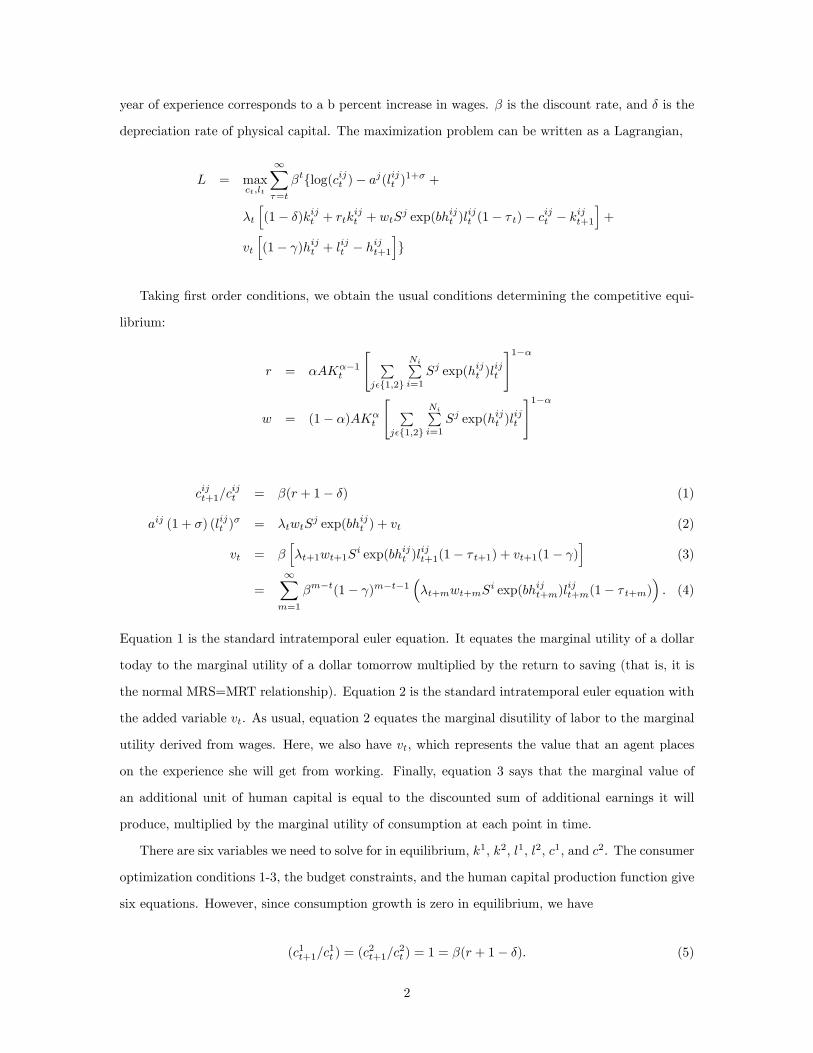
year of experience corresponds to a b percent increase in wages. � is the discount rate, and � is the

depreciation rate of physical capital. The maximization problem can be written as a Lagrangian,

L = maxct;lt

1X�=t

�tflog(cijt )� aj(lijt )

1+� +

�t

h(1� �)kijt + rtk

ijt + wtS

j exp(bhijt )lijt (1� � t)� c

ijt � k

ijt+1

i+

vt

h(1� )hijt + l

ijt � h

ijt+1

ig

Taking �rst order conditions, we obtain the usual conditions determining the competitive equi-

librium:

r = �AK��1t

" Pj�f1;2g

NiPi=1

Sj exp(hijt )lijt

#1��

w = (1� �)AK�t

" Pj�f1;2g

NiPi=1

Sj exp(hijt )lijt

#1��

cijt+1=cijt = �(r + 1� �) (1)

aij (1 + �) (lijt )� = �twtS

j exp(bhijt ) + vt (2)

vt = �h�t+1wt+1S

i exp(bhijt )lijt+1(1� � t+1) + vt+1(1� )

i(3)

=1Xm=1

�m�t(1� )m�t�1��t+mwt+mS

i exp(bhijt+m)lijt+m(1� � t+m)

�: (4)

Equation 1 is the standard intratemporal euler equation. It equates the marginal utility of a dollar

today to the marginal utility of a dollar tomorrow multiplied by the return to saving (that is, it is

the normal MRS=MRT relationship). Equation 2 is the standard intratemporal euler equation with

the added variable vt. As usual, equation 2 equates the marginal disutility of labor to the marginal

utility derived from wages. Here, we also have vt; which represents the value that an agent places

on the experience she will get from working. Finally, equation 3 says that the marginal value of

an additional unit of human capital is equal to the discounted sum of additional earnings it will

produce, multiplied by the marginal utility of consumption at each point in time.

There are six variables we need to solve for in equilibrium, k1, k2, l1, l2, c1, and c2. The consumer

optimization conditions 1-3, the budget constraints, and the human capital production function give

six equations. However, since consumption growth is zero in equilibrium, we have

(c1t+1=c1t ) = (c

2t+1=c

2t ) = 1 = �(r + 1� �): (5)

2

So two of the equations are identical, and we only have 5 equations de�ning the six unknowns.

Intuitively, the overall capital stock is determined by equation 5 , but the capital held by each agent

is undetermined. No matter what quantity of capital an agent holds, as long as the return on

capital is such that equation 5 holds, the agent will not change her capital holdings.2 Therefore,

rather than solving the problem of each agent individually, we solve the associated social planning

problem. As markets in this model are complete and there are no externalities, the social planning

solution will replicate the competitive allocation. We are not modeling the wealth distribution, so

we are unconcerned with the speci�c capital holdings of individuals; we only wish to model the

aggregate capital stock.3

A.2 Social planning problem

The social planner solves the following problem with weights on the consumers N1 and N2(1� ).

Without loss of generality, we herein set N1 = N2 = 1

maxc1t ;c

2t l1t ;l

2t

1X�=t

�t� �log(c1)� a1(l1)1+�

�+ (1� )

�log(c2)� a2(l2)1+�

�subject to the resource constraint and human capital production function,

AtK�t (S

1�h1t�"l1t + S

2�h2t�"l2t )

1�� = Kt+1 � (1� �)Kt + c1t + c

2t

hit+1 = (1� )hit + lit; i � f1; 2g:

The social planning problem can be written as a Lagrangian,

L = maxct;lt

1X�=t

�tf �log(c1)� a1(l1)1+�

�+ (1� )

�log(c2)� a2(l2)1+�

��t�AtK

�t (S

1 exp(bh1t )l1t + S

2 exp(bh2t )l2t )1�� �Kt+1 + (1� �)Kt � c1t � c2t

�+

v1t�(1� �)h1t + l1t � h1t+1

�+

v2t�(1� �)h2t + l2t � h2t+1

�g:

2That is, there is one degree of freedom in the capital holdings of the two agents.3 In order to solve for the competitive allocation, we would need to impose initial capital holdings. This is equivalent

to the choice of weights on the the utility of the di¤erent types of agents in the social planning problem.

3

We can take �rst-order conditions for the 7 variables of interest (K, c1, c2, l1, l2, h1, h2) and 3

Lagrange multipliers,

C1 : �t = ��c1t��

(6)

C2 : �t = (1� �)�c2t�� t

(7)

L1 : �a1(1� l1t )� = �t(1� �)S1�h1t�"AtK

�t (S

1�h1t�"l1t + S

2�h2t�"l2t )

�� + �1t (8)

L2 : (1� �)a2(1� l2t )� = �t(1� �)S2�h2t�"AtK

�t (S

1�h1t�"l1t + S

2�h2t�"l2t )

�� + �2t (9)

Kt+1 : �t = ��t+1��AtK

��1t (S1h1t l

1t + S

2h2t l2t )1�� + 1� �

�(10)

H1t+1 : �1t = �

264 �t+1"�h1t+1

�"�1At(1� �)S1l1t+1K�

t+1(S1�h1t+1

�"l1t+1

+S2�h2t+1

�"l2t+1)

�� + (1� �)�1t+1

375 (11)

H2t+1 : �2t = �

264 �t+1"�H2t

�"�1A(1� �)S2L2t+1K�

t (S1�H1t

�"L1t

+S2�H2t

�"L2t )

�� + (1� �)�2t+1

375 (12)

As usual, the social planner�s optimization conditions are analogous to those of individual agents.

Equations 8 and 9 are the intratemporal euler equations corresponding to equation 2. As before, the

marginal disutility of an extra hour of work is set equal to the marginal value of the dollars earned

plus the marginal value of the human capital produced. Equation 10 is the standard intertemporal

euler equation. As we can see, capital holdings of each agent are undetermined �there is simply an

aggregate stock of capital. Finally, equations 11 and 12 correspond to equation 3. Again, they tell

us that the value of a unit of human capital is equal to the discounted value of the additional output

it will produce in the future.

A.3 Calibration and Simulation

There are 6 parameters that need to be calibrated in order to use the model to predict the e¤ects of

employment. �, is, as usual, set to .33. The discount rate, �, is set to .97. The depreciation rates

of capital and experience, � and , respectively, are set to .03.

The return to experience has been estimated in a number of papers, including Blau and Kahn

(1997), Topel (1991), Topel and Ward (1992), and Olivetti (2006). Looking across these papers, we

take 5 percent returns to be a reasonable approximation. In general, analysts �nd decreasing returns

to experience. Since we allow experience to depreciate, this creates decreasing returns. A person

with zero experience who works one year will gain one year of experience. A person who starts with

10 years of experience and works one more year will only end up with 10.7 years of experience after

4

losing .3 years to depreciation. This creates curvature similar to that found by labor economists.

Finally, we need to calibrate the male-female wage gap. We simply average the estimates of the

wage gap by country from Pissarides et al. (2006, pg 76) weighting by each country�s share in total

EU employment. This gives an estimated average wage gap of 15.12 percent.

The last two unknown parameters are a1 and a2, corresponding to the disutility of labor for

men and women. In order to simulate the model, we simply �nd the pair fa1; a2g (using matlab�s

unconstrained optimization algorithm) that replicates actual employment rates seen at various points

in time. Speci�cally, we �nd pairs of a�s for 1985, 1990, 1995, 2000, and 2005. We assume the

economy begins in steady state in 1985, and then simulate the model forward taking into account

the changes in the parameters every 5 years. The model is simulated using Dynare.

5

Figure 1.  Trend in Output per Hour, Output per Capita, and Hours per Capita, US and EU‐15, Annual Growth Rates, 1970‐

2006

0

1

2

3

4

5

6

1970 1975 1980 1985 1990 1995 2000 2005

Percent

EU‐15 Y/H

US Y/H

‐3

‐2

‐1

0

1

2

3

4

1970 1975 1980 1985 1990 1995 2000 2005

Percent

US Y/NEU‐15 Y/N

US H/N

EU‐15 H/N

Source:  GGDC Total Economy Database except BEA, BLS for the United States, see data appendix

Figure 2.  Trend in Employment per Capita and Hours per Employee, US and EU‐15, Annual Growth Rates, 1970‐2006

‐1

‐0.5

0

0.5

1

1.5

2

1970 1975 1980 1985 1990 1995 2000 2005

Percent

EU‐15 E/N

US E/N

‐2

‐1.5

‐1

‐0.5

0

0.5

1

1970 1975 1980 1985 1990 1995 2000 2005

Percent

US H/E

EU‐15 H/E

Source:   GGDC Total Economy Database except BLS for the United States, see data appendix

Figure 3. Trend in Capital Input per Hour and Total Factor Productivity, US and EU‐15, Annual Growth Rates, 1980‐2004

0

1

2

3

4

5

6

7

1980 1985 1990 1995 2000

Percent

EU‐15 K/H

US K/H

‐2

‐1.5

‐1

‐0.5

0

0.5

1

1.5

2

2.5

1980 1985 1990 1995 2000

Percent

EU‐15 TFP

US TFP

Source:   EU‐KLEMS Database, see data appendix

Source: Authorsʹ calculations

Figure 4: Employment and Share effects for the Turnaround in Employment per Capita Growth, 1995‐2005 versus 1985‐1995

Mediterranean

‐0.02 ‐0.015 ‐0.01 ‐0.005 0 0.005 0.01 0.015 0.02

15‐24

25‐34

35‐44

45‐54

55‐64

65+

15‐24

25‐34

35‐44

45‐54

55‐64

65+

Nordic

15‐24

25‐34

35‐44

45‐54

55‐64

65+

15‐24

25‐34

35‐44

45‐54

55‐64

65+

Employment Effect

Share Effect

Men

Women

Anglo‐Saxon

15‐24

25‐34

35‐44

45‐54

55‐64

65+

15‐24

25‐34

35‐44

45‐54

55‐64

65+

Continental

‐0.02 ‐0.015 ‐0.01 ‐0.005 0 0.005 0.01 0.015 0.02 0.025

15‐24

25‐34

35‐44

45‐54

55‐64

65+

15‐24

25‐34

35‐44

45‐54

55‐64

65+

Source:   Bassanini‐Duval (2006) weighted by employment from GGDC Total Economy Database

Figure 5: EU‐15 Employment‐Weighted Tax Wedge, EPL, PMR, ARR, Union Density and High Corporatism, 1978‐2003

Tax Wedge

30

31

32

33

34

35

36

37

1978 1983 1988 1993 1998 2003

Union Density

26

30

34

38

42

1978 1983 1988 1993 1998 2003

ARR

22

24

26

28

30

32

34

1978 1983 1988 1993 1998 2003

EPL

2

2.2

2.4

2.6

2.8

3

1978 1983 1988 1993 1998 2003

PMR

1

2

3

4

5

6

1978 1983 1988 1993 1998 2003

High Corporatism

0.3

0.4

0.5

0.6

1978 1983 1988 1993 1998 2003

Source:  Authorʹs Calculations

Simulations, 1994=100, 1980‐2003Figure 6: EU‐15 Men and Women Employment per Capita

Women

90

95

100

105

110

115

120

1981 1983 1985 1987 1989 1991 1993 1995 1997 1999 2001 2003

Fixed Policy

Predicted

No Post‐1995 Dummy

Men

80

85

90

95

100

105

110

115

120

1981 1983 1985 1987 1989 1991 1993 1995 1997 1999 2001 2003

Fixed Policy

Predicted

No Post‐1995 Dummy

Source:  Authorʹs Calculations

Figure 7: Actual, Predicted, and Fixed‐Policy Labor Productivityand Employment, 1994=100, 1980‐2003

Labor Productivity

88

90

92

94

96

98

100

102

1980 1982 1984 1986 1988 1990 1992 1994 1996 1998 2000 2002

Actual

Counterfactual

Predicted

Employment

96

98

100

102

104

106

108

110

112

1980 1982 1984 1986 1988 1990 1992 1994 1996 1998 2000 2002

Actual

Counterfactual

Predicted

1970‐1995 1995‐2006 Difference 1970‐1995 1995‐2006 Difference 1970‐1995 1995‐2006 Difference

United States 1.42 2.13 0.71 0.55 ‐0.04 ‐0.58 1.97 2.09 0.12EU‐15 2.89 1.41 ‐1.49 ‐0.82 0.59 1.41 2.07 2.00 ‐0.07EU‐15xMed 2.81 1.87 ‐0.94 ‐0.84 0.07 0.92 1.97 1.94 ‐0.03

Nordic 2.41 2.09 ‐0.32 ‐0.77 0.56 1.33 1.64 2.66 1.02Denmark   2.74 1.15 ‐1.59 ‐0.85 0.67 1.52 1.89 1.82 ‐0.07Finland  3.29 2.48 ‐0.80 ‐1.27 0.97 2.24 2.02 3.45 1.44Sweden  1.72 2.49 0.76 ‐0.41 0.26 0.68 1.31 2.75 1.44

Anglo‐Saxon 2.73 2.18 ‐0.55 ‐0.72 0.46 1.18 2.01 2.64 0.63Ireland 4.03 4.16 0.13 ‐0.66 2.01 2.67 3.37 6.17 2.80United Kingdom 2.68 2.04 ‐0.64 ‐0.72 0.37 1.09 1.96 2.41 0.45

Continental 2.88 1.75 ‐1.14 ‐0.89 ‐0.13 0.76 1.99 1.62 ‐0.37Austria 3.12 2.28 ‐0.85 ‐0.66 ‐0.18 0.48 2.46 2.09 ‐0.37Belgium 2.85 1.42 ‐1.43 ‐0.68 0.50 1.17 2.17 1.92 ‐0.25France 3.05 1.85 ‐1.19 ‐1.15 ‐0.16 0.99 1.90 1.70 ‐0.20Germany 2.91 1.67 ‐1.23 ‐0.96 ‐0.33 0.63 1.94 1.34 ‐0.60Luxembourg 2.50 1.92 ‐0.58 0.29 1.28 0.99 2.78 3.20 0.41Netherlands 2.30 1.54 ‐0.76 ‐0.54 0.47 1.01 1.76 2.01 0.25Portugal 2.85 1.70 ‐1.15 0.16 0.05 ‐0.11 3.01 1.75 ‐1.26

Mediterranean 3.15 0.24 ‐2.91 ‐0.75 1.92 2.67 2.40 2.15 ‐0.25Greece 2.36 2.53 0.17 ‐0.33 1.13 1.46 2.03 3.66 1.63Italy  2.71 0.44 ‐2.28 ‐0.43 0.74 1.16 2.29 1.18 ‐1.11Spain 4.19 ‐0.24 ‐4.43 ‐1.35 3.69 5.04 2.84 3.46 0.61

Standard Deviation 0.63 1.00 # 0.46 1.02 # 0.55 1.27

Source :  GGDC Total Economy Database except BEA for the United States, see data appendix

Growth Rates Growth Rates Growth Rates

Table 1

Growth in Output per Hour, Hours per Capita, and Output per Capita,Countries and Country Groups, selected intervals, 1970‐2006

Labour Productivity Hours per Capita Output per Capita

United States EU‐15 Nordic Anglo‐Saxon Continental Mediterranean1980‐1995 Growth RatesLabour Productivity (Y/H) 1.34 2.34 2.30 2.46 2.46 2.07Hours per Employee (H/E) ‐0.13 ‐0.49 ‐0.02 ‐0.16 ‐0.77 ‐0.32Employent per Capita (E/N) 0.51 ‐0.04 ‐0.74 ‐0.23 0.03 0.11Capital per Hour (K/H) 3.56 3.68 4.06 4.44 3.47 3.52Capital Deepening 1.17 1.11 1.23 1.25 1.07 1.05Total Factor Productivity (TFP) 0.17 1.23 1.07 1.21 1.39 1.02

1995‐2004 Growth RatesLabour Productivity (Y/H) 2.29 1.41 1.92 2.11 1.63 0.63Hours per Employee (H/E) ‐0.16 ‐0.39 ‐0.16 ‐0.37 ‐0.57 ‐0.29Employent per Capita (E/N) 0.06 0.92 0.56 1.01 0.49 1.73Capital per Hour (K/H) 3.56 2.81 2.86 3.99 2.99 2.01Capital Deepening 1.20 0.95 0.96 1.20 1.01 0.73Total Factor Productivity (TFP) 1.09 0.46 0.96 0.91 0.63 ‐0.10

Difference, 1995‐2004 minus 1980‐1995Labour Productivity (Y/H) 0.95 ‐0.93 ‐0.37 ‐0.34 ‐0.82 ‐1.44Hours per Employee (H/E) ‐0.03 0.10 ‐0.14 ‐0.21 0.20 0.03Employent per Capita (E/N) ‐0.46 0.95 1.30 1.24 0.46 1.62Capital per Hour (K/H) ‐0.01 ‐0.87 ‐1.20 ‐0.45 ‐0.48 ‐1.51Capital Deepening 0.03 ‐0.16 ‐0.27 ‐0.05 ‐0.06 ‐0.32Total Factor Productivity (TFP) 0.92 ‐0.77 ‐0.11 ‐0.29 ‐0.76 ‐1.12

Memo Items:Capital‐Output Ratio (K/Y) ‐0.96 0.06 ‐0.82 ‐0.10 0.34 ‐0.07Capital per Capita (K/N) ‐0.49 0.18 ‐0.04 0.59 0.18 0.15

Source :  EU‐KLEMS Database, see data appendix

Table 2

Annual Growth Rates and Turnaround in Growth Rates of Labour Productivity, Labour and Capital Ratios, and Total Factor Productivity, Countries and Country Groups, 1980‐2004

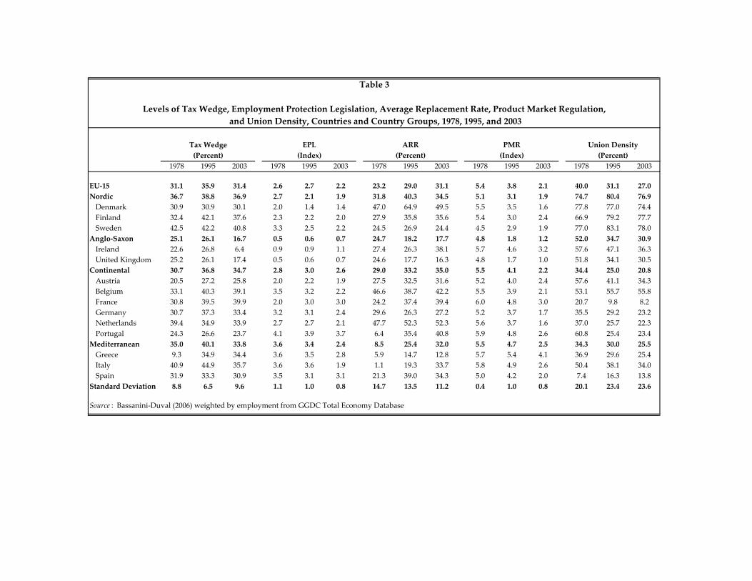
1978 1995 2003 1978 1995 2003 1978 1995 2003 1978 1995 2003 1978 1995 2003

EU‐15 31.1 35.9 31.4 2.6 2.7 2.2 23.2 29.0 31.1 5.4 3.8 2.1 40.0 31.1 27.0Nordic 36.7 38.8 36.9 2.7 2.1 1.9 31.8 40.3 34.5 5.1 3.1 1.9 74.7 80.4 76.9Denmark   30.9 30.9 30.1 2.0 1.4 1.4 47.0 64.9 49.5 5.5 3.5 1.6 77.8 77.0 74.4Finland  32.4 42.1 37.6 2.3 2.2 2.0 27.9 35.8 35.6 5.4 3.0 2.4 66.9 79.2 77.7Sweden  42.5 42.2 40.8 3.3 2.5 2.2 24.5 26.9 24.4 4.5 2.9 1.9 77.0 83.1 78.0

Anglo‐Saxon 25.1 26.1 16.7 0.5 0.6 0.7 24.7 18.2 17.7 4.8 1.8 1.2 52.0 34.7 30.9Ireland 22.6 26.8 6.4 0.9 0.9 1.1 27.4 26.3 38.1 5.7 4.6 3.2 57.6 47.1 36.3United Kingdom 25.2 26.1 17.4 0.5 0.6 0.7 24.6 17.7 16.3 4.8 1.7 1.0 51.8 34.1 30.5

Continental 30.7 36.8 34.7 2.8 3.0 2.6 29.0 33.2 35.0 5.5 4.1 2.2 34.4 25.0 20.8Austria 20.5 27.2 25.8 2.0 2.2 1.9 27.5 32.5 31.6 5.2 4.0 2.4 57.6 41.1 34.3Belgium 33.1 40.3 39.1 3.5 3.2 2.2 46.6 38.7 42.2 5.5 3.9 2.1 53.1 55.7 55.8France 30.8 39.5 39.9 2.0 3.0 3.0 24.2 37.4 39.4 6.0 4.8 3.0 20.7 9.8 8.2Germany 30.7 37.3 33.4 3.2 3.1 2.4 29.6 26.3 27.2 5.2 3.7 1.7 35.5 29.2 23.2Netherlands 39.4 34.9 33.9 2.7 2.7 2.1 47.7 52.3 52.3 5.6 3.7 1.6 37.0 25.7 22.3Portugal 24.3 26.6 23.7 4.1 3.9 3.7 6.4 35.4 40.8 5.9 4.8 2.6 60.8 25.4 23.4

Mediterranean 35.0 40.1 33.8 3.6 3.4 2.4 8.5 25.4 32.0 5.5 4.7 2.5 34.3 30.0 25.5Greece 9.3 34.9 34.4 3.6 3.5 2.8 5.9 14.7 12.8 5.7 5.4 4.1 36.9 29.6 25.4Italy  40.9 44.9 35.7 3.6 3.6 1.9 1.1 19.3 33.7 5.8 4.9 2.6 50.4 38.1 34.0Spain 31.9 33.3 30.9 3.5 3.1 3.1 21.3 39.0 34.3 5.0 4.2 2.0 7.4 16.3 13.8

Standard Deviation 8.8 6.5 9.6 1.1 1.0 0.8 14.7 13.5 11.2 0.4 1.0 0.8 20.1 23.4 23.6

Source :  Bassanini‐Duval (2006) weighted by employment from GGDC Total Economy Database

(Percent)(Percent) (Index) (Percent) (Index)

Table 3

Levels of Tax Wedge, Employment Protection Legislation, Average Replacement Rate, Product Market Regulation, and Union Density, Countries and Country Groups, 1978, 1995, and 2003

Tax Wedge EPL ARR PMR Union Density

Δ Tax Wedge ‐0.28 *** ‐0.21 ** ‐0.37 ***Δ Employment Protection Legislation  0.25 0.34 ‐0.14Δ Product Market Regulation  ‐0.55 ‐0.29 ‐0.75Δ Average Replacement Rate ‐0.17 *** ‐0.11 ** ‐0.27 ***Δ Union Density ‐0.47 *** ‐0.41 *** ‐0.56 ***Δ Output Gap  0.51 *** 0.56 *** 0.46 ***Δ High Corportism ‐2.76 ** ‐1.87 * ‐4.2 ***Post‐1995 Time Effect 0.95 *** 1.09 *** 0.66 ***

R2 0.47 0.47 0.37N 314 312 312RMSE 1.32 1.34 1.65

Weighted by Population Yes Yes YesFixed Effects Yes Yes Yes

* Indicates significance at 10% level, ** 5%, *** 1%.  Fixed effects coefficients not reported.†  Time dummy equal to 1 if within 1996‐2003, otherwise 0‡ Δ = 2 year average change 

Source:  Bassanini‐Duval (2006) and OECD, see data appendix

Table 4

on Policy and Institutional Variables, 1980‐2003 Regressions of Employment per Capita Growth

Combined Men Women

‡

†

Δ Tax Wedge ‐0.38 *** ‐0.28 *** ‐0.25 *** ‐0.15 **Δ Employment Protection Legislation  ‐0.20 0.86 1.57 * 0.27Δ Product Market Regulation  ‐1.11 * ‐0.44 0.66 ‐0.05Δ Average Replacement Rate ‐0.21 *** ‐0.18 *** ‐0.13 ** ‐0.18 ***Δ Union Density ‐0.43 *** ‐0.46 *** ‐0.45 *** ‐0.41 ***Δ High Corporatism  ‐2.27 ** ‐2.04 ** ‐1.70 * ‐1.59 *Δ Output Gap  0.54 *** 0.52 *** 0.51 *** 0.38 ***Post‐1995 Time Effect 0.94 *** 0.86 *** 1.15 ***

R2 0.46 0.52 0.48 0.59N 320 320 320 320RMSE 1.25 1.18 1.31 1.09

Weighted by Population Yes Yes No YesFixed Effects Yes Yes Yes YesTime Dummy for Every Year No No No Yes

* Indicates significance at 10% level, ** 5%, *** 1%.  Time and fixed effects coefficients not reported.†  Time dummy equal to 1 if within 1996‐2003, otherwise 0‡ Δ = 2 year average change 

Source: Authorʹs Calculations

Table 5

First‐Stage Regressions of Employment per Capita Growth on Policy

(4)

and Institutional Variables, 1980‐2003

(1) (2) (3)

‡

†

LP PredictionActual Predicted Difference Actual Predicted Difference Incl. K/N Residual LP K/N

Nordic ‐0.45 ‐0.59 0.14 0.33 ‐0.01 0.34 ‐0.48 0.25 0.05Anglo‐Saxon ‐0.22 ‐0.12 ‐0.1 0.31 0.06 0.25 ‐0.04 0.23 ‐0.03Continental ‐0.71 ‐0.10 ‐0.61 ‐0.07 ‐0.05 ‐0.02 ‐0.11 0.01 ‐0.02Mediterranean ‐1.44 ‐0.78 ‐0.66 ‐0.02 0.40 ‐0.42 ‐0.92 0.79 0.11

Source :  Authorsʹ calculations

Table 6

Turnarounds in Labour Productivity and Capital Per Capita, 1995‐2005 versus 1985‐2005

LP turnaround K/N turnaround Post‐2005 Acceleration

Employment Rate ‐0.84 *** ‐0.64 *** ‐0.74 *** ‐0.64 *** ‐0.63 *** ‐0.62 ***Δ Tax Wedge ‐0.04Δ Employment Protection Legislation  1.82 *** 1.66 *** 1.77 *** 1.62 ** 1.07 1.19 *Δ Product Market Regulation  0.48 0.56 0.54 0.58 0.98 * 0.8Δ Average Replacement Rate 0.10 *** 0.14 *** 0.12 *** 0.13 *** 0.13 ** 0.14 ***Δ Union Density ‐0.06 0.03 ‐0.02Δ High Corporatism  ‐0.94 ‐0.49 ‐0.73Δ Output Gap  0.78 *** 0.68 *** 0.73 *** 0.67 *** 0.74 *** 0.76 ***Post‐1995 Time Effect 0.06 ‐0.14 ‐0.14 0.15

R2 0.65 0.63 0.64 0.62 0.52 0.69N 320 320 320 320 320 320RMSE 0.92 0.95 0.93 0.95 1.18 0.86

Weighted by Population Yes Yes Yes Yes No YesFixed Effects Yes Yes Yes Yes Yes YesTime Dummy for Every Year No No No No No YesExogenous Instrument(s) None

* Indicates significance at 10% level, ** 5%, *** 1%.  Time and fixed effects coefficients not reported.†  Time dummy equal to 1 if within 1996‐2003, otherwise 0‡ Δ = 2 year average change 

Source: Authorʹs Calculations

(5) (6)

Table 7

Second‐Stage Regressions of Productivity Growth on Employment per CapitaGrowth and Policy and Institutional Variables, 1980‐2003

(1) (2) (3) (4)

Tax wedge Tax wedge Tax wedge Tax wedgePost‐1995 TE High Corp. High Corp. High Corp.

Union Dens. Union Dens. Union Dens.

Tax wedge

‡

†

Actual Predicted Fixed Policy Policy Effect Actual Predicted Fixed Policy Policy EffectPre‐95 2.53 2.12 1.82 0.30 ‐0.27 0.06 0.35 ‐0.29

Mediterranean Post‐95 0.52 0.90 1.18 ‐0.28 1.87 1.63 1.46 0.17Change ‐2.01 ‐1.23 ‐0.65 ‐0.58 2.14 1.57 1.11 0.46

Pre‐95 2.26 2.38 2.41 ‐0.03 ‐0.04 ‐0.12 ‐0.28 0.16Continental Post‐95 1.76 1.57 1.75 ‐0.18 0.76 0.92 0.80 0.12

Change ‐0.50 ‐0.81 ‐0.66 ‐0.15 0.80 1.04 1.08 ‐0.04

Pre‐95 2.00 2.33 2.27 0.06 ‐0.61 ‐0.80 ‐0.64 ‐0.17Nordic Post‐95 1.92 1.38 1.80 ‐0.41 0.70 1.02 0.73 0.29

Change ‐0.08 ‐0.95 ‐0.47 ‐0.47 1.31 1.82 1.36 0.46

Pre‐95 2.52 2.56 3.14 ‐0.57 ‐0.23 ‐0.25 ‐0.92 0.67Anglo‐Saxon Post‐95 2.23 2.13 2.57 ‐0.44 0.83 0.86 0.26 0.60

Change ‐0.29 ‐0.43 ‐0.57 0.13 1.06 1.12 1.18 ‐0.07

Pre‐95 2.32 2.33 2.39 ‐0.06 ‐0.15 ‐0.15 ‐0.28 0.13EU‐15 Post‐95 1.44 1.44 1.73 ‐0.29 1.16 1.16 0.91 0.25

Change ‐0.88 ‐0.89 ‐0.66 ‐0.23 1.31 1.31 1.19 0.12

Source: Authorsʹ Calculations

Table 8 

Actual, Predicted, and Counterfactual Simulations of Productivity and Employment Growth

Labor Productivity Employment per Capita

Shock Size Employment Productivity Output Per Capita

Tax Wedge 9.21 ‐2.67 1.71 ‐0.96(0.64) (0.53) (0.4)

Employment 0.87 0.74 0.23 0.97Protection Legislation (0.36) (0.37) (0.31)

Product Market Regulation 0.9 ‐0.14 0.35 0.21(0.24) (0.25) (0.22)

Average Replacement Rate 11.31 ‐0.90 1.37 0.47(0.34) (0.31) (0.25)

Union Density 23.32 ‐7.93 5.07 ‐2.85(1.17) (1.23) (1.07)

High Corpratism  1 ‐1.02 0.65 ‐0.37(0.48) (0.33) (0.21)

Note: Standard errors (Delta method) in parentheses

Source: Authorsʹ Calculations

Table 9

Productivity, and Output per Capita Effects of Unit Standard Deviation Policy Shocks on Employment