the role of learning for asset prices, business cycles and
TRANSCRIPT
The Role of Learning for Asset Prices, Business Cyclesand Monetary Policy
Fabian Winkler∗
30 December 2014(click here to access latest version)
Abstract
The importance of financial frictions for the business cycle is widely recognised,but what is less recognised is that the results obtained from studying these frictionsdepend heavily on the underlying asset pricing theory. I examine the implications oflearning-based asset pricing for business cycles with financial frictions. I constructa model in which stock market valuations affect firms’ ability to access credit, andin which investors rely on past observation to predict the future. Learning greatlyimproves asset price properties such as return volatility and predictability. In combin-ation with financial frictions, a powerful feedback loop emerges between beliefs, stockprices and real activity, leading to substantial amplification of shocks. The model-implied subjective expectations are found to be consistent with patterns of forecasterror predictability in survey data. A reaction of monetary policy to asset prices sta-bilises expectations and substantially improves welfare, which is not the case underrational expectations.
Keywords: Learning, Asset Pricing, Credit Constraints, Monetary Policy, Survey DataJEL Classification: D83, E32, E44, E52
∗Centre for Macroeconomics and London School of Economics, Houghton Street, London WC2A 2AE,[email protected]. I thank my advisor Wouter den Haan for his invaluable guidance and support;Klaus Adam, Johannes Boehm, Peter Karadi, Albert Marcet, Stéphane Moyen, Rachel Ngai, MichaelPeters, Markus Riegler, and participants at the ECB-CFS-Bundesbank lunchtime seminar, SingaporeManagement University, Econometric Society Winter Meeting in Madrid, Symposium of the SAEe inPalma de Mallorca, EEA Annual Meeting in Toulouse, and LBS Transatlantic Doctoral Conference, foruseful comments and suggestions.

1 Introduction
I think financial factors in general, and asset prices in particular, play a more centralrole in explaining the dynamics of the economy than is typically reflected in macro-economic models, even after the experience of the crisis.- Andrew Haldane, 30 April 2014
The above statement, made by the Chief Economist of the Bank of England during aparliamentary hearing, may provoke disbelief among macroeconomists. After all, a wealthof research in the last fifteen years has been dedicated precisely to the links betweenthe financial sector and the real economy. Financial frictions are now seen as a centralmechanism by which asset prices interact with macroeconomic dynamics.
Still, our understanding of this interaction remains incomplete, in part due to the inherentdifficulty of modelling asset prices.
The typical business cycle model employs an asset pricing theory based on time-separablepreferences with moderate degrees of risk aversion and rational expectations. Such anasset pricing theory is well known to be inadequate for many empirical regularities such asreturn volatility (Shiller, 1981) and return predictability (Fama and French, 1988). Thisis not problematic when asset prices are disconnected from the real economy, since assetpricing and business cycle dynamics can then be separated.1 In the presence of financialfrictions however, the prices of assets used as collateral affect borrowing constraints andhence the dynamics of the economy. A failure to generate realistic endogenous asset pricedynamics can then become a potentially important source of model misspecification.
This paper examines the business cycle implications of a learning-based asset pricing the-ory. I construct a model of firm credit frictions in which agents are unable to form rationalexpectations about the price of equities in the stock market, and instead have to learn frompast observation to form subjective beliefs. The learning-based approach to stock pricinghas been shown to perform surprisingly well in endowment economies, without the needto rely on non-separable preferences or habit (Adam, Marcet and Nicolini, 2013; Adam,Beutel and Marcet, 2014). The interpretation of price dynamics under learning is quitedifferent from rational expectations. With learning, stock prices fluctuate not because ofvariations in the discounting of prices and returns, but because of variations in subjectivebeliefs about the prices and returns themselves. The deviation of these subjective beliefsfrom rational expectations is a natural measure of “price misalignments”, “over-” and“undervaluation”. These notions are often present in informal arguments about financialmarkets, but absent in most asset pricing theories.2
1For the real business cycle model with recursive preferences, Tallarini Jr. (2000) showed that businesscycle properties are driven almost entirely by the intertemporal elasticity of substitution, while asset priceproperties are almost entirely governed by the degree of risk aversion.
2For example, in October 2014, the IMF warned of “highly correlated mispricing [..] across assets“ inits Global Financial Stability Report (p. 6).
1

A second model ingredient is that firms are subject to credit constraints, the tightnessof which depends on firm market value. This type of constraint emerges from a limitedcommitment problem in which defaulting firms can be restructured and resold (similar toChapter 11 of the US Bankruptcy Code) as opposed to being liquidated. It provides amechanism by which high stock market valuations translate into easier access to credit.The model has a “financial accelerator” mechanism similar to Bernanke et al. (1999), withthe strength and properties of this mechanism crucially depending on the endogenousdynamics of stock prices.
The analysis of the model yields three results. First, a positive feedback loop emergesbetween beliefs, asset prices and the production side of the economy, which leads to con-siderable amplification and propagation of business cycle shocks. When investor beliefsare more optimistic, their demand for stocks increases. This increases firm valuations andrelaxes credit conditions. This in turn allows firms to move closer to their profit optimum.Provided counteracting general equilibrium forces are not too strong, they will also be ableto pay higher dividends to their shareholders, raising stock prices further and propagatinginvestor optimism even more. The financial accelerator mechanism becomes much morepowerful than under rational expectations. At the same time, the learning mechanismgreatly improves asset price properties such as price and return volatility and predictabil-ity without the need to impose complex preferences or high degrees of risk aversion. Thisresult suggests that the relatively weak quantitative strength of the financial acceleratoreffect in many existing models (Cordoba and Ripoll, 2004) is at least in part due to lowendogenous asset price volatility.
Second, while agents’ subjective expectations are not rational expectations, they are con-sistent in a number of ways with data obtained from surveys. I document that forecasterrors on several macroeconomic aggregates (from the US Survey of Professional Fore-casters) as well as on stock returns (from the Duke-Fuqua CFO Survey) can be predictedby the price/dividend ratio as well as forecast revisions. This is also true in the model,despite the fact that learning only adds one free parameter to the model and agents havemodel-consistent expectations for all relevant prices and outcomes except for stock prices.When they are over-predicting asset prices, they also over-predict credit limits dependingon those prices and therefore aggregate activity, just like in the data.
Third, I show that the model has important normative implications. A recurring questionin monetary economics is whether policy should react to asset price “misalignments”. Gali(2014) writes that justifying such a reaction requires “the presumption that an increasein interest rates will reduce the size of an asset price bubble” for which “no empiricalor theoretical support seems to have been provided”. This paper is a first step towardsfilling this gap. Indeed, I find that under learning, the welfare-maximising monetary policywithin a class of interest rate rules reacts strongly to asset price growth. By raising interestrates when stock prices are rising, policy is able to curb the endogenous build-up of over-optimistic investor beliefs. Such a reaction reduces both asset price volatility and business
2
cycle volatility. In contrast, under rational expectations, a policy reaction to asset pricesdoes not improve welfare, in line with earlier findings in the literature.
The remainder of this paper is structured as follows. Section 2 reviews the related literat-ure. Section 3 provides several empirical facts relating to the macroeconomic effects andproperties of stock prices as well as discrepancies of measured expectations from rationalexpectations. Section 4 presents a highly stylised version of the model that permits ananalytic solution. It shows that credit frictions or asset price learning alone does notgenerate either amplification of shocks or interesting asset price dynamics, while theircombination does. The full model which can be used for quantitative analysis is thenpresented in Section 5. Section 6 contains the quantitative results. Section 7 contains themonetary policy analysis. Section 8 concludes.
2 Related literature
This paper starts from learning-based asset pricing developed in a series of papers by KlausAdam and Albert Marcet (Adam and Marcet, 2011; Adam et al., 2013, 2014). They showthat parsimonious models of learning about stock prices succeed in explaining key aspectsof observed stock price data such as the excess volatility, equity premium, and returnpredictability puzzles. They also show consistency with investor expectations, which arehard to reconcile with rational expectations. Recent work by Barberis et al. (forthcoming)goes in a similar direction. While these papers study endowment economies, I take theirapproach to an economy with production. This allows one to look at the interactionsbetween financial markets and the real economy, as well as policy implications.
There exist other approaches to asset pricing in production economies. For models withfinancial frictions in particular, it is popular to simply include exogenous shocks to explainthe observed fluctuations in asset prices. Iacoviello (2005) and Liu et al. (2013), for ex-ample, set up economies in which exogenous shocks to housing demand drive house prices,which in turn affect credit constraints, and study the financial accelerator mechanism. Xuet al. (2013) have a model with a credit friction similar to that in my model, in whichborrowing limits also depend on stock market valuations. They prove the existence ofrational liquidity bubbles and introduce a shock that governs the size of this bubble, thusenabling them to match the stock prices seen in the data. In all of these models, the simplepreferences and rational expectations would not allow realistic asset price dynamics in theabsence of asset price shocks, and the structural interpretation of these shocks is often notclear.3 In order to advance our understanding of the interaction between asset prices andthe real economy, I believe that it is necessary to have macroeconomic models that canendogenise asset price fluctuations. This paper is a step in this direction.
3Even the disaster-risk model of Gourio (2012) can be interpreted as such a model in which exogenousshocks to discount factors drive asset prices, even though quantities are not affected by financial frictionsbut by the changes in discount factors themselves.
3

The macro-finance literature has two main, rational expectations-based propositions toobtain realistic asset price dynamics. The first one is due to Campbell and Cochrane(1999) and relies on a non-linear form of habit formation combined with high risk aver-sion. The second, so-called “long-run risk” approach due to Bansal and Yaron (2004),introduces small, predictable and observable components to long-run consumption anddividend growth combined with Epstein-Zin preferences. There are some papers that tryto embed these alternative approaches in production economies: Boldrin et al. (2001) forhabit formation, Tallarini Jr. (2000) and Croce (2014) for long-run risk. These papersconsider real business cycle models and are mainly concerned with endogenising con-sumption and dividend streams in a production economy while preserving the asset priceimplications. To my knowledge, there are no studies which take either approach to largerbusiness cycle models with financial frictions, possibly because they are computationallyquite demanding. They also require the use of preferences which have some rather counter-intuitive properties (shown by Lettau and Uhlig (2000) for habit and Epstein et al. (2013)for long-run risk). In my view, learning-based asset pricing is a promising alternative. It isintuitively appealing to think that asset prices are to some degree driven by self-amplifyingwaves of over- and under-confidence, and such a view is supported by survey evidence.Importantly, it also has implications for policy, as this paper shows.
The paper also makes a contribution to the literature on adaptive learning in businesscycles. A number of papers in this area have studied learning in combination with financialfrictions (Caputo, Medina and Soto, 2010; Milani, 2011; Gelain, Lansing and Mendicino,2013). The conventional approach taken in this literature consists of two steps: first,derive the linearised equilibrium conditions of the economy under rational expectations;second, replace all terms involving expectations with parametrised forecast functions, andupdate the parameters using recursive least squares every period. Such models certainlyproduce very rich dynamics, but they are problematic on several grounds. First, it is notclear that first-order conditions parametrised in this way correspond in a meaningful senseto intertemporal optimisation problems.4 Second, these models are often very complexand intransparent. The need to parametrise every expectation in the first-order conditionsrequires a large number of parameters. In all but the simplest models, it then becomesprohibitively difficult to analyse equilibrium dynamics. In this paper, I propose a moretransparent and parsimonious approach. Beliefs are restricted to be model-consistent asunder rational expectations (with the only exception being the beliefs about stock prices)and agents make optimal choices given this set of beliefs. Even in a medium-sized DSGEmodel, the introduction of learning then adds only one parameter and one state variableto the model.
Finally, the paper also relates to the debate on whether monetary policy should react to4In any model with an Euler equation, for example, some version of the stochastic discount factor needs
to be learned by the agents, an object which depends on their own choices. It is unclear how an agentwould be able to select a choice based on an intertemporal first-order condition and at the same time notunderstand how he makes choices when forming expectations.
4

asset price “misalignments”. Bernanke and Gertler (2001) found in a financial frictionsmodel with rational exogenous asset price bubbles that the answer is “no”. This view,although not unchallenged (Filardo, 2001; Cecchetti et al., 2002), forms the consensusopinion and indeed the practice of most central banks. It has also recently been reinforcedby Gali (2014), who argues that since rational bubbles are predicted to grow at the rate ofinterest, the optimal policy to deflate a bubble might even be to lower interest rates whenasset prices are rising too fast. Without incorporating bubbles, Faia and Monacelli (2007)find a similar result, and conclude that a strong exclusive anti-inflationary stance remainswelfare-maximising. This paper shows that such policy recommendations depend criticallyon the underlying asset price theory. In a world of less than fully rational expectations,raising interest rates in an asset price boom can be effective in curbing exuberant investorexpectations and mitigate a surge (and subsequent reversal) in real activity due to highasset prices and easy access to credit.
3 Empirical evidence
The purpose of this section is to document three sets of facts. First, movements in the ag-gregate stock market have sizeable effects on investment and credit constraints, consistentwith the credit friction in my model. Second, stock price movements exhibit high volatil-ity and return predictability. Third, measures of expectations from survey data, both forstock prices and macro variables, reveal systematic deviations from rational expectations.Some but not all of these observations have been documented previously in the literature.
3.1 Effect of the stock market on investment and credit constraints
One of the oldest documented links between financial markets and the real economy is thatthe stock market predicts investment (Barro, 1990). Of course, prediction does not implycausation. It is plausible that new information about improved economic fundamentalscauses both stock prices and investment to rise, with stock prices responding faster. Thisview is taken by Beaudry and Portier (2006) who show that in an estimated vector errorcorrection model, innovations in stock prices orthogonal to current changes in TFP predicta substantial portion of long-run TFP variation. This suggests that stock price fluctuationsare in fact “news shocks” about future productivity. However, it is also conceivable thatstock market movements have a direct effect on investment even when they do not reflectchanging expectations about the economic fundamentals. Blanchard et al. (1993) constructa measure of expected fundamentals and find that stock prices retain their predictivepower even when controlling for fundamentals. In general though, it is hard to come toany definitive conclusions about causality without spelling out a structural model.
In the model of this paper, higher stock prices affect investment because of financialfrictions: Firms with higher market value have easier access to external finance and can
5
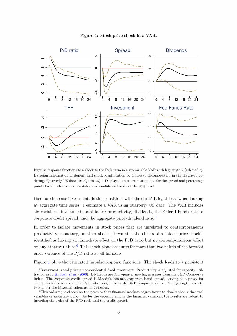
Figure 1: Stock price shock in a VAR.0
24
68
−10
−5
05
−1
01
2
−.2
0.2
.4
−.5
0.5
11.5
−.4
−.2
0.2
0 4 8 12 16 20 24 0 4 8 12 16 20 24 0 4 8 12 16 20 24
0 4 8 12 16 20 24 0 4 8 12 16 20 24 0 4 8 12 16 20 24
P/D ratio Spread Dividends
TFP Investment Fed Funds Rate
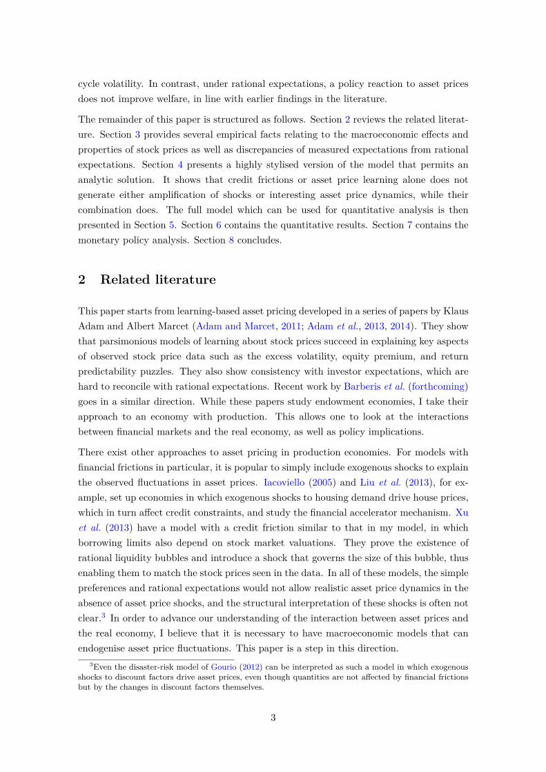
Impulse response functions to a shock to the P/D ratio in a six-variable VAR with lag length 2 (selected byBayesian Information Criterion) and shock identification by Cholesky decomposition in the displayed or-dering. Quarterly US data 1962Q1-2012Q4. Displayed units are basis points for the spread and percentagepoints for all other series. Bootstrapped confidence bands at the 95% level.
therefore increase investment. Is this consistent with the data? It is, at least when lookingat aggregate time series. I estimate a VAR using quarterly US data. The VAR includessix variables: investment, total factor productivity, dividends, the Federal Funds rate, acorporate credit spread, and the aggregate price/dividend-ratio.5
In order to isolate movements in stock prices that are unrelated to contemporaneousproductivity, monetary, or other shocks, I examine the effects of a “stock price shock”,identified as having an immediate effect on the P/D ratio but no contemporaneous effecton any other variables.6 This shock alone accounts for more than two thirds of the forecasterror variance of the P/D ratio at all horizons.
Figure 1 plots the estimated impulse response functions. The shock leads to a persistent5Investment is real private non-residential fixed investment. Productivity is adjusted for capacity util-
isation as in Kimball et al. (2006). Dividends are four-quarter moving averages from the S&P Compositeindex. The corporate credit spread is Moody’s baa-aaa corporate bond spread, serving as a proxy forcredit market conditions. The P/D ratio is again from the S&P composite index. The lag length is set totwo as per the Bayesian Information Criterion.
6This ordering is chosen on the premise that financial markets adjust faster to shocks than either realvariables or monetary policy. As for the ordering among the financial variables, the results are robust toinverting the order of the P/D ratio and the credit spread.
6
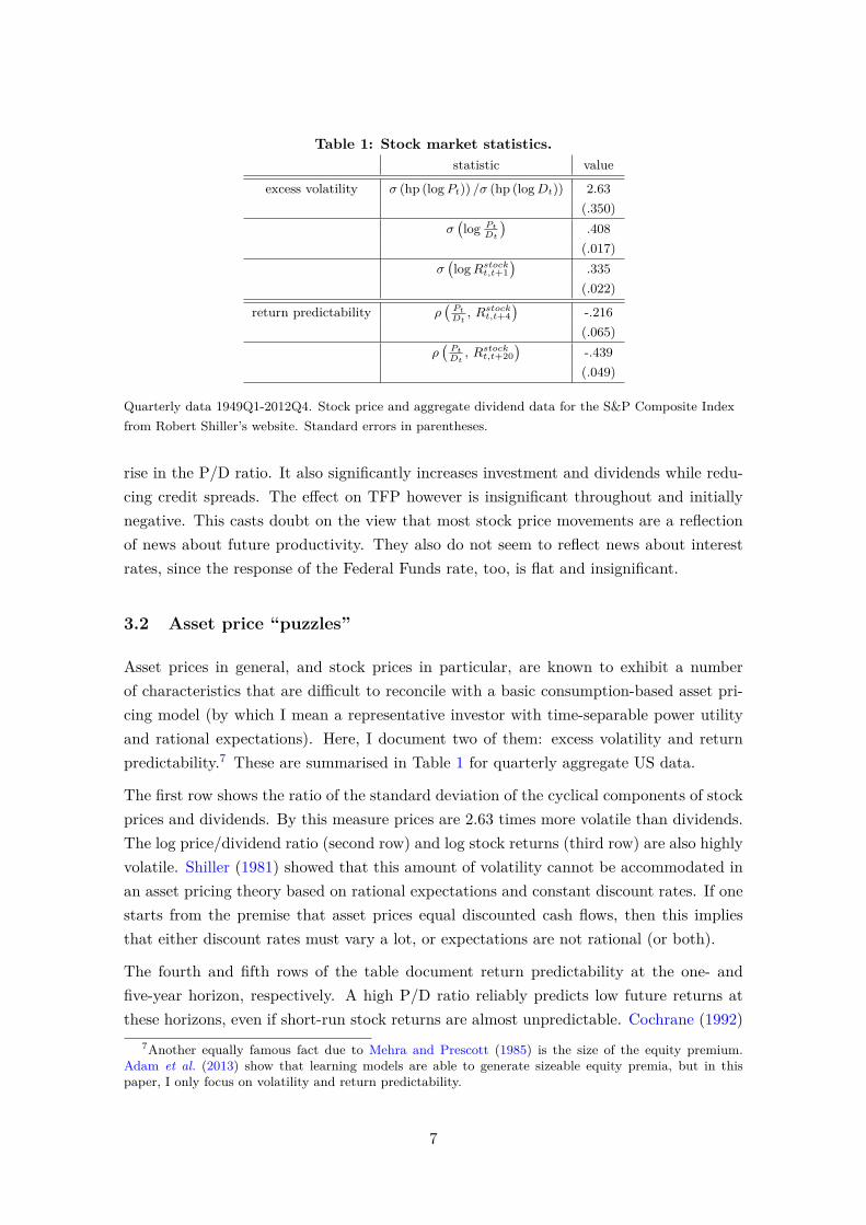
Table 1: Stock market statistics.statistic value
excess volatility σ (hp (logPt)) /σ (hp (logDt)) 2.63(.350)
σ(log Pt
Dt
).408(.017)
σ(logRstockt,t+1
).335(.022)
return predictability ρ(PtDt, Rstockt,t+4
)-.216(.065)
ρ(PtDt, Rstockt,t+20
)-.439(.049)
Quarterly data 1949Q1-2012Q4. Stock price and aggregate dividend data for the S&P Composite Indexfrom Robert Shiller’s website. Standard errors in parentheses.
rise in the P/D ratio. It also significantly increases investment and dividends while redu-cing credit spreads. The effect on TFP however is insignificant throughout and initiallynegative. This casts doubt on the view that most stock price movements are a reflectionof news about future productivity. They also do not seem to reflect news about interestrates, since the response of the Federal Funds rate, too, is flat and insignificant.
3.2 Asset price “puzzles”
Asset prices in general, and stock prices in particular, are known to exhibit a numberof characteristics that are difficult to reconcile with a basic consumption-based asset pri-cing model (by which I mean a representative investor with time-separable power utilityand rational expectations). Here, I document two of them: excess volatility and returnpredictability.7 These are summarised in Table 1 for quarterly aggregate US data.
The first row shows the ratio of the standard deviation of the cyclical components of stockprices and dividends. By this measure prices are 2.63 times more volatile than dividends.The log price/dividend ratio (second row) and log stock returns (third row) are also highlyvolatile. Shiller (1981) showed that this amount of volatility cannot be accommodated inan asset pricing theory based on rational expectations and constant discount rates. If onestarts from the premise that asset prices equal discounted cash flows, then this impliesthat either discount rates must vary a lot, or expectations are not rational (or both).
The fourth and fifth rows of the table document return predictability at the one- andfive-year horizon, respectively. A high P/D ratio reliably predicts low future returns atthese horizons, even if short-run stock returns are almost unpredictable. Cochrane (1992)
7Another equally famous fact due to Mehra and Prescott (1985) is the size of the equity premium.Adam et al. (2013) show that learning models are able to generate sizeable equity premia, but in thispaper, I only focus on volatility and return predictability.
7
shows that the variance of the P/D ratio can be decomposed into its covariance with futurereturns and future dividend growth. Since dividend growth is not very volatile, not wellpredicted by the P/D ratio, and the P/D ratio itself is volatile, it follows that returnsmust be predictable. Assuming rational expectations, Cochrane identifies the predictablecomponent of returns with a time-varying discount rate. Again, the alternative is thatexpectations used to price assets are distinct from rational expectations. In the model ofthis paper, a high P/D ratio is not a result of low required returns, but of high expectedreturns - where the subjective expectation is distinct from the statistical prediction.
3.3 Survey data on expectations
The rational expectations hypothesis is a fundamental building block of modern macroe-conomics. Sometimes, it is criticised as an unrealistic modelling device which asserts thatagents are hyper-rational, endowed with infinite computing power and knowledge of thestructural shocks and relationships of the economy. But in fact, it makes no such claim.In the words of Sargent (2008), it simply asserts that “outcomes do not differ systematic-ally [...] from what people expect them to be”. Put differently, any agent’s forecast errorshould not be predictable by information available to the agent at the time of the forecast.
The rational expectations hypothesis is testable based on survey measures of expectations.It is almost always rejected. Here, I document some of these tests, and characterise someof the predictability patterns of forecast errors.
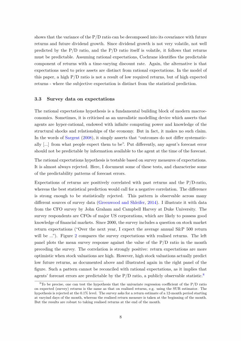
Expectations of returns are positively correlated with past returns and the P/D-ratio,whereas the best statistical prediction would call for a negative correlation. The differenceis strong enough to be statistically rejected. This pattern is observable across manydifferent sources of survey data (Greenwood and Shleifer, 2014). I illustrate it with datafrom the CFO survey by John Graham and Campbell Harvey at Duke University. Thesurvey respondents are CFOs of major US corporations, which are likely to possess goodknowledge of financial markets. Since 2000, the survey includes a question on stock marketreturn expectations (“Over the next year, I expect the average annual S&P 500 returnwill be ...”). Figure 2 compares the survey expectations with realised returns. The leftpanel plots the mean survey response against the value of the P/D ratio in the monthpreceding the survey. The correlation is strongly positive: return expectations are moreoptimistic when stock valuations are high. However, high stock valuations actually predictlow future returns, as documented above and illustrated again in the right panel of thefigure. Such a pattern cannot be reconciled with rational expectations, as it implies thatagents’ forecast errors are predictable by the P/D ratio, a publicly observable statistic.8
8To be precise, one can test the hypothesis that the univariate regression coefficient of the P/D ratioon expected (survey) returns is the same as that on realised returns, e.g. using the SUR estimator. Thehypothesis is rejected at the 0.1% level. The survey asks for a return estimate of a 12-month period startingat varyind days of the month, whereas the realised return measure is taken at the beginning of the month.But the results are robust to taking realised returns at the end of the month.
8
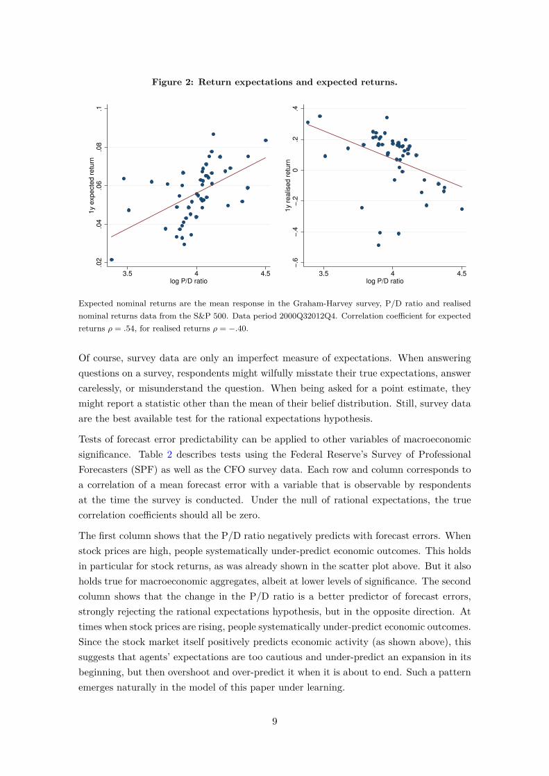
Figure 2: Return expectations and expected returns..0
2.0
4.0
6.0
8.1
1y e
xpecte
d r
etu
rn
3.5 4 4.5log P/D ratio
−.6
−.4
−.2
0.2
.41y r
ealis
ed r
etu
rn
3.5 4 4.5log P/D ratio
Expected nominal returns are the mean response in the Graham-Harvey survey, P/D ratio and realisednominal returns data from the S&P 500. Data period 2000Q32012Q4. Correlation coefficient for expectedreturns ρ = .54, for realised returns ρ = −.40.
Of course, survey data are only an imperfect measure of expectations. When answeringquestions on a survey, respondents might wilfully misstate their true expectations, answercarelessly, or misunderstand the question. When being asked for a point estimate, theymight report a statistic other than the mean of their belief distribution. Still, survey dataare the best available test for the rational expectations hypothesis.
Tests of forecast error predictability can be applied to other variables of macroeconomicsignificance. Table 2 describes tests using the Federal Reserve’s Survey of ProfessionalForecasters (SPF) as well as the CFO survey data. Each row and column corresponds toa correlation of a mean forecast error with a variable that is observable by respondentsat the time the survey is conducted. Under the null of rational expectations, the truecorrelation coefficients should all be zero.
The first column shows that the P/D ratio negatively predicts with forecast errors. Whenstock prices are high, people systematically under-predict economic outcomes. This holdsin particular for stock returns, as was already shown in the scatter plot above. But it alsoholds true for macroeconomic aggregates, albeit at lower levels of significance. The secondcolumn shows that the change in the P/D ratio is a better predictor of forecast errors,strongly rejecting the rational expectations hypothesis, but in the opposite direction. Attimes when stock prices are rising, people systematically under-predict economic outcomes.Since the stock market itself positively predicts economic activity (as shown above), thissuggests that agents’ expectations are too cautious and under-predict an expansion in itsbeginning, but then overshoot and over-predict it when it is about to end. Such a patternemerges naturally in the model of this paper under learning.
9

Table 2: Forecast error predictability: Correlation coefficients.
(1) (2) (3)
forecast variable logPDt ∆ logPDt forecast revision
Rstockt,t+4 -.44*** .06 n/a
(-3.42) (.41)
Yt+3 -.21* .22** .29***
(-1.78) (2.42) (3.83)
It+3 -.20* .25*** .31***
(-1.74) (2.88) (3.79)
Ct+3 -.19* .21** .23***
(-1.85) (2.37) (2.67)
ut+3 .05 -.27*** .43***
(.12) (-3.07) (6.07)
Correlation coefficients for mean forecast errors on one-year ahead nominal stock returns (Graham-Harveysurvey) and three-quarter ahead real output growth, investment growth, consumption growth and theunemployment rate (SPF). t-statistics for the null of zero correlation in parentheses. One, two, and threeasterisks correspond to significance at the 10%, 5%, and 1% levels. Regressors: Column (1) is the S&P500 P/D ratio and Column (2) is its first difference. Column (3) is the forecast revision as in Coibionand Gorodnichenko (2010). Data from Graham-Harvey covers 2000Q3-2012Q4. Data for the SPF covers1981Q1-2012Q4.
The third column reports the results of a particular test of rational expectations devised byCoibion and Gorodnichenko (2010). Since for any variable xt, the SPF asks for forecasts atone- through four-quarter horizon, it is possible to construct a measure of agent’s revisionof the change in xt as Et [xt+3 − xt] − Et−1 [xt+3 − xt]. Forecast errors are positivelypredicted by this revision measure. Coibion and Gorodnichenko take this as evidence forsticky information models in which information sets are gradually updated over time. AsI will show later, it is also consistent with the learning model developed in this paper.
4 Understanding the mechanism
In this section, I construct a simplified version of the model which illustrates the inter-action between asset prices and credit frictions under learning. I impose several strongassumptions permitting a closed-form solution. Quantitative analysis will require a richermodel, the development of which is relegated to the next section. The main message ofthis section is that financial frictions alone do not generate either sizeable amplification ofbusiness cycle shocks or asset price volatility, but in combination with learning they do.
10

4.1 Model setup
Time is discrete at t = 0, 1, 2, . . . . The model economy consists of a representative house-hold and a representative firm. The representative household is risk-neutral and inelast-ically supplies one unit of labour. Its utility maximisation programme is as follows:
max(Ct,St,Bt)∞t=0
EP∞∑t=0
βtCt
s.t. Ct + StPt +Bt = wt + St−1 (Pt +Dt) +Rt−1Bt−1
St ∈[0, S
], S−1, B−1
Ct is the amount of non-durable consumption goods purchased by the household in periodt. The consumption good is traded in a competitive spot market and serves as thenuméraire. wt is the real wage rate. Labour is also traded in a competitive spot market,so that the wage wt is taken as given by the household. Moreover, the household can tradetwo financial assets, again in competitive spot markets: one-period bonds, denoted by Btand paying gross real interest Rt in the next period; and stocks St which trade at price Ptand entitle their holder to dividend payments Dt. The household cannot short-sell stocksand his maximum stock holdings are capped at some S > 1.9
The household maximises the expectation of discounted future consumption under theprobability measure P. This measure is the subjective belief system held by agents in themodel economy at time t, which will be discussed in detail further below. The first orderconditions describing the household’s optimal plan under an arbitrary P are
Rt = R = β−1 (4.1)
St
= 0 if Pt > βEPt [Pt+1 +Dt+1]
∈[0, S
]if Pt = βEPt [Pt+1 +Dt+1]
= S if Pt < βEPt [Pt+1 +Dt+1]
. (4.2)
Let us now turn to the firm. It engages in the production of a good which can be usedboth for consumption and investment. It is produced using capital Kt−1, which the firmowns, and labour Lt according to the constant returns to scale technology
Yt = Kαt−1 (AtLt)1−α (4.3)
9The constraint on St is necessary to guarantee existence of the learning equilibrium, although it neverbinds along the equilibrium path.
11

where At is its productivity. Here, I only allow for permanent shocks to productivity:
logAt = logG+ logAt−1 + εt, εt ∼ N(−σ
2
2 , σ2)iid (4.4)
In particular, the expected growth rate of productivity is constant at EtAt+1/At ≡ G. Thecapital stock is predetermined and owned by the firm. It depreciates at the rate δ at theend of each period. The firm can also issue shares and bonds as described above. Thus,its period budget constraint reads as follows:
Yt + (1− δ)Kt−1 +Bt + StPt = wtLt +Kt + St−1 (Pt +Dt) +RBt−1 (4.5)
Before describing the equilibrium, it is useful to introduce the marginal return on capital:
Rkt = ∂Yt∂Kt−1
+ 1− δ (4.6)
4.2 Frictionless equilibrium
In the absence of financial constraints, the Modigliani-Miller theorem will render the com-position of firm financing redundant and the model collapses to a standard stochasticgrowth model. In particular, the optimal choice of the capital stock (under rational ex-pectations) equates the marginal return on capital with the inverse of the discount factor:EtRkt+1 = β−1. Whatever one assumes about the financial structure of the firm, its totalvalue will equal the size of the capital stock. The capital stock and firm value co-movesperfectly with productivity:
Kt/At = Kt = K∗ (4.7)Pt +BtAt
= Kt = K∗ (4.8)
where K∗ = G(
αβ−1−1+δ
)1/(1−α)e−ασ
2/2.
4.3 Rational expectations equilibrium with financial frictions
In introducing financial frictions, I impose constraints on both the equity and debt in-struments. On the equity side, the firm is not allowed to change the quantity of sharesoutstanding, fixed at St = 1. Further, it is not allowed to use retained earnings to financeinvestment. Instead, all earnings net of interest and depreciation have to be paid out toshareholders:
Dt = Yt − wtLt − δKt−1 − (R− 1)Bt−1 (4.9)
12
Combined with equation (4.5), this assumption implies that the firm’s capital stock mustbe entirely debt-financed: Kt = Bt at all t.10 In other words, the firm’s book value ofequity after dividend payouts is constrained to be zero. This does not mean, however, thatthe market value of equity is also zero as long as the firm’s expected dividend payouts arestrictly positive.
On the debt side, the level of debt that can be acquired by the firm is limited to a fractionξ ∈ [0, 1] of the total market value of its assets, i.e. the sum of debt and equity:
Bt ≤ ξ (Bt + Pt)
⇔ Kt ≤ξ
1− ξPt (4.10)
Equation (4.10) is a simple constraint on leverage, i.e. debt divided by value of total assets.I depart from the standard assumption that total assets enter with their liquidation value(in this case Kt, the book value) and instead let them enter with their market value (inthis case Bt + Pt). This captures the idea that a firm which is more highly valued byfinancial markets will have easier access to credit. This could be because high marketvalue acts as a signal to lenders for the firm’s ability to repay, or because the amountlenders can recover in the event of default depends on the price at which a firm can beresold to other financial market participants. In the full version of the model in the nextsection, I formally derive (4.10) from a limited commitment problem.
The firm maximises the presented discounted sum of future dividends, using the householddiscount factor:
max(Kt,Lt,Dt)∞t=0
E∞∑t=0
βtDt
s.t. Dt = Yt − wtLt + (1− δ −R)Kt−1
Kt ≤ξ
1− ξPt
Kt ≥ 0, K−1
In particular, it makes its decisions under the same belief system Pt as the household.Due to constant returns to scale in production, we can write dividends at the optimum asfollows:
maxLt
Dt =(Rkt −R
)Kt−1 (4.11)
The optimal choice of capital is to exhaust borrowing limits as long as the expected internal10This holds under the suitable initial condition K−1 = B−1, e.g. the firm starts with zero book value
of equity on its balance sheet. This assumption is relaxed in the full model.
13
return on capital exceeds the external return paid to creditors:
Kt
= 0 if EtRkt+1 < R
∈[0, ξ
1−ξPt]
if EtRkt+1 = R
= ξ1−ξPt if EtRkt+1 > R
(4.12)
When solving for the equilibrium, market clearing needs to be imposed. The marketclearing condition for bonds is just R = β−1. That for equity is St = 1, which means theEuler equation (4.2) has to hold with equality:
Pt = βEt [Pt+1 +Dt+1] (4.13)
Goods market clearing requires
Yt +Kt = C + (1− δ)Kt−1 (4.14)
and labour market clearing requires Lt = 1.
The equilibrium under rational expectations admits a closed-form solution. First, notethat the equilibrium return on capital depends on the aggregate capital stock due todecreasing returns to scale at the aggregate level:
Rkt = Rk(Kt−1, εt
)= α
(Geεt
Kt−1
)1−α
+ 1− δ (4.15)
This dependency comes about through a general equilibrium effect: A higher level of thecapital stock increases labour demand, which increases real wages and therefore lowersthe return on capital. Next, one can write expected dividends as a function of the capitalstock:
D(kt, Kt
)= Et
[Dt+1At
]=(EtRk
(Kt, εt+1
)−R
)kt (4.16)
Here, I have made a distinction between the capital choice kt of the representative firmthat takes future wages as given, and the aggregate capital stock Kt which determineswages and the return on capital in general equilibrium. Of course, in equilibrium thetwo are equal. Finally, the effective stock price under rational expectations is simply thediscounted sum of future dividends:
Pt = PtAt
= βEt∞∑s=0
βsAt+sAt
D(Kt+s, Kt+s
)(4.17)
First, let us consider the case ξ = 1. In this case, Kt is constant across time and states inequilibrium and is at its efficient level K∗ such that EtRk (K∗, εt+1) = R. By consequence,expected dividends and the market value of equity are zero: D (K∗,K∗) = 0 and Pt = 0.Intuitively, when the firm can borrow up to the total amount of its market value, it faces
14
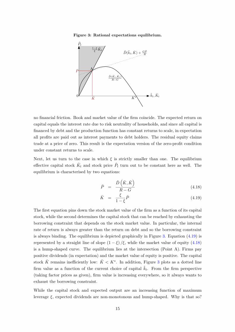
Figure 3: Rational expectations equilibrium.
kt, Kt
1−ξξ Kt
D(Kt,Kt)R−G
K K∗
P
0
A
Pt
D(kt, K) + GPR
no financial friction. Book and market value of the firm coincide. The expected return oncapital equals the interest rate due to risk neutrality of households, and since all capital isfinanced by debt and the production function has constant returns to scale, in expectationall profits are paid out as interest payments to debt holders. The residual equity claimstrade at a price of zero. This result is the expectation version of the zero-profit conditionunder constant returns to scale.
Next, let us turn to the case in which ξ is strictly smaller than one. The equilibriumeffective capital stock Kt and stock price Pt turn out to be constant here as well. Theequilibrium is characterised by two equations:
P =D(K, K
)R−G
(4.18)
K = ξ
1− ξ P (4.19)
The first equation pins down the stock market value of the firm as a function of its capitalstock, while the second determines the capital stock that can be reached by exhausting theborrowing constraint that depends on the stock market value. In particular, the internalrate of return is always greater than the return on debt and so the borrowing constraintis always binding. The equilibrium is depicted graphically in Figure 3. Equation (4.19) isrepresented by a straight line of slope (1− ξ) /ξ, while the market value of equity (4.18)is a hump-shaped curve. The equilibrium lies at the intersection (Point A). Firms paypositive dividends (in expectation) and the market value of equity is positive. The capitalstock K remains inefficiently low: K < K∗. In addition, Figure 3 plots as a dotted linefirm value as a function of the current choice of capital kt. From the firm perspective(taking factor prices as given), firm value is increasing everywhere, so it always wants toexhaust the borrowing constraint.
While the capital stock and expected output are an increasing function of maximumleverage ξ, expected dividends are non-monotonous and hump-shaped. Why is that so?
15

There are two opposing forces affecting expected dividends, as can be seen from thefollowing decomposition:
d
dξD(K, K
)=
EtRk (K, εt+1)−R︸ ︷︷ ︸
>0
+EtdRk
dK
(K, εt+1
)K︸ ︷︷ ︸
<0
dKdξ︸︷︷︸>0
(4.20)
The first term in brackets captures a partial equilibrium effect, which is internalised bythe firm. When a firm is financially constrained, its internal rate of return is higherthan the return it has to pay to debt holders. By borrowing more, it can increase itsscale of production and make more profit. The second term, however, captures a generalequilibrium effect: higher investment lowers the marginal product of capital, which inpractice is realised through an increase in the equilibrium wage wt+1. When ξ is small(financial frictions are severe) the partial equilibrium effect dominates, while for a large ξthe general equilibrium effect dominates.
Most importantly however, financial frictions do not lead to any amplification or propaga-tion of shocks in the rational expectations equilibrium. They have a level effect on output,capital, etc., but the dynamics of the model are identical for any value of ξ. This can beseen by looking at the variances of log stock price and output growth which do not dependon ξ:
Var [∆ logPt] = σ2 (4.21)
Var [∆ log Yt] =(1− 2α+ 2α2
)σ2 (4.22)
Intuitively, with financial frictions, a shock to productivity raises asset prices just as muchas to allow the firm to instantly adjust the capital stock proportionately.
At the same time, the model cannot replicate many of the stylised facts on stock pricedata. Up to a first-order approximation, the relative volatility of asset price growth withrespect to dividend growth is bounded from below:
σ (∆ logPt)σ (∆ logDt)
<(1− 2α+ 2α2
)1/2≤√
2 (4.23)
The asset price volatility observed in the data can therefore not be matched. The volatilityof the price/dividend ratio can also not be matched: in fact, the forward P/D ratio is evenconstant:
PDt = PtEtDt+1
≡ 1R−G
(4.24)
Furthermore, excess returns are unpredictable: Et [(Pt+1 +Dt+1) /Pt]−R = 0. Finally, bydefinition of rational expectations, forecast errors are unpredictable, again at odds withthe data.
16

4.4 Learning equilibrium
I now describe the equilibrium under learning. Qualitatively, this alteration to the expect-ation formation process can address many of the issues encountered in the last section: itwill increase the volatility of stock prices, account for return and forecast error predict-ability, and most importantly, induce endogenous amplification and propagation on theproduction side of the model economy. The only departure from rational expectations willbe that agents do not understand the pricing function that maps fundamentals into anequilibrium stock price. Instead, they form subjective beliefs about the law of motion ofprices and update them using realised price observations.
More specifically, agents continue to make optimal choices for a consistent belief systemgoverned by the measure P. The equilibrium therefore satisfies “internal rationality” asformalised by Adam and Marcet (2011) and used in Eusepi and Preston (2011). I imposethe following restrictions to beliefs. Under P,
1. agents observe the exogenous productivity process (εt)∞t=0 and have correct beliefsabout its distribution;
2. agents believe that Pt evolves according to
logPt − logPt−1 = µt + ηt (4.25)
µt = µt−1 + νt (4.26)
where(ηt
νt
)∼ N
(−1
2
(σ2η
σ2ν
),
(σ2η 0
0 σ2ν
))iid, (4.27)
the variable µt and the disturbances ηt and νt are unobserved and the prior aboutµt in period 0 is given by
µ0 | F0 ∼ N(µ0, σ
2µ
)where σ2
µ =−σ2
ν +√σ4ν + 4σ2
νσ2η
2 ; (4.28)
3. agents update their beliefs about µt after making their choices and observing equi-librium prices in period t;
4. for any model variable xt , any future date t + τ , and any sequence of exogen-ous productivity shocks εt, . . . , εt+τ and stock prices Pt, . . . , Pt+τ which lies on theequilibrium path:
EPt [xt+τ | εt, Pt, . . . , εt+τ , Pt+τ ] = xt+τ a.s.
i.e. agents’ beliefs are correct conditional on the realisation of stock prices andfundamentals.
17
The first assumption implies that agents have as much information about the fundamentalshocks of the economy as under rational expectations. The second assumption amounts tosaying that agents believe stock prices to be a random walk. This random walk is believedto have a small, unobservable, and time-varying drift µt. Learning about this drift is goingto be the key driver of asset price dynamics. The third assumption imposes that forecastsof stock prices are updated after equilibrium prices are determined, so as to avoid possiblemultiple equilibria in price and forecast determination.11
To the best of my knowledge, the fourth and final assumption is novel to the learningliterature. To make their choices, agents must form expectations about more than justthe stock price and the exogenous processes of the economy. For example, investors needto form a belief about dividends, which are endogenous and depend on wages and thecapital choice of the firm in equilibrium. The typical way to deal with this is to intro-duce additional expectation formation processes for all forecast endogenous variables. Myview is that this increases complexity to the point of rendering a learning model opaque.Instead, I retain the simplicity of rational expectationsas much as possible: Conditionalon a realisation of stock prices and fundamentals on the equilibrium path, agents do notmake systematic forecast errors. In particular, the choices they make are conditionallyconsistent with equilibrium outcomes. I also solve for these beliefs in much the same wayas one would under rational expectations; the procedure is discussed in Section 5 and Ap-pendix C. The only difference to rational expectations lies in the word “conditional”. Sinceagents’ beliefs about stock prices produce biased forecast errors, their unconditional fore-casts about other endogenous variables EPt [xt+1] are also biased, even if the conditionalforecasts EPt [xt+1 | εt+1, Pt+1] are not.
Despite such relatively accurate beliefs, agents are still left with the important problem ofmaking a good guess about the unobservable drift µt of stock prices. Optimal Bayesianbelief updating amounts to Kalman filtering in this case, since (4.25)-(4.28) is a linearstate-space system. Under P, agents’ beliefs about µt at time t are normally distributedwith stationary variance σ2
µ and mean µt−1. This belief about the mean of µt, which I willusually just call “the belief”, evolves according to the updating equation:
µt = µt−1 −σ2ν
2 + g
(logPt − logPt−1 +
σ2η + σ2
ν
2 − µt−1
)(4.29)
In this equation, Pt and Pt−1 are observed, realised stock prices. These are determined inequilibrium under the actual law of motion of the economy and do not follow the perceivedlaw of motion described by (4.25)-(4.28). The parameter g is called the “learning gain”. Itgoverns the speed with which agents move their prior in the direction of the last forecasterror.12 When g is high, agents are confident that observed changes in the growth rate
11This “lagged belief updating” is common in the learning literature. It makes all feedback betweenforecasts and prices inter- rather than intramporal. For further discussion see Adam et al. (2014).
12The gain is related to the variances of the disturbances by the formula g = 12
(σ2ν
σ2ε
+√
σ4ν
σ4ε
+ 4σ2ν
σ2ε
),
18

of asset prices are due to changes in the trend µt rather than the noise ηt. The gain isnot decreasing in time: Agents believe that the drift in asset prices is itself time-varying,so that even after a long period of time it remains difficult to forecast it. A consequenceof this is that beliefs never converge: Agents always entertain the possibility of somestructural change to the law of motion of asset prices, so that even an infinite number ofobservations is not completely informative about the future.
It is important to keep in mind that the disturbances ηt and νt are objects that exist onlyin the subjective belief system P. The actual equilibrium under learning does not containany shock process other than the productivity shock εt. Instead, the equilibrium stillcontains the actual market clearing conditions (4.13) and (4.14), even if they are unknownto the agents. By Walras’ law, it is sufficient to impose stock market clearing. Under P,(4.13) reads as follows:
Pt = EPt Pt+1 + EPt Dt+1R
(4.30)
=Pt exp
(µt−1 + 1
2σ2µ
)+AtD
(Kt, Kt
)R
(4.31)
= AtD(Kt, Kt
)R− exp
(µt−1 + 1
2σ2µ
) (4.32)
The second line is obtained by substituting in agents’ beliefs about the evolution of thefuture stock price EtPt+1 and dividends EtDt+1. Under P, agents forecast future dividendsaccurately conditional on their belief about stock prices. Therefore, their expectationsabout dividends depend on the current capital stock in the same way as under rationalexpectations.
In sum, the learning equilibrium is the solution to the following:
Pt =D(Kt, Kt
)R− exp
(µt−1 + 1
2σ2µ
) (4.33)
Kt = ξ
1− ξ Pt (4.34)
µt = µt−1 −σ2ν
2 + g
(log Pt
Pt−1+ logG+ εt − µt−1 +
σ2η + σ2
ν
2
)(4.35)
The first two equations are static and the third is dynamic. The third equation alsodepends on the productivity innovation εt, and as such Pt and Kt are not constant anymore. The resulting stock price dynamics after a positive innovation at t = 1 are depictedin Figure 4.13 The initial shock at t = 1 raises stock prices proportional to productivity. Inthe rational expectations equilibrium, this would be all that happens. Learning investorsand is strictly increasing in the signal-to-noise ratio σ2
ν/σ2ε .
13The figure depicts the case in which beliefs start at their rational expectations value µt = logG andsubjective uncertainty is vanishing in the sense that σ2
ν , σ2η → 0 while g remains constant.
19
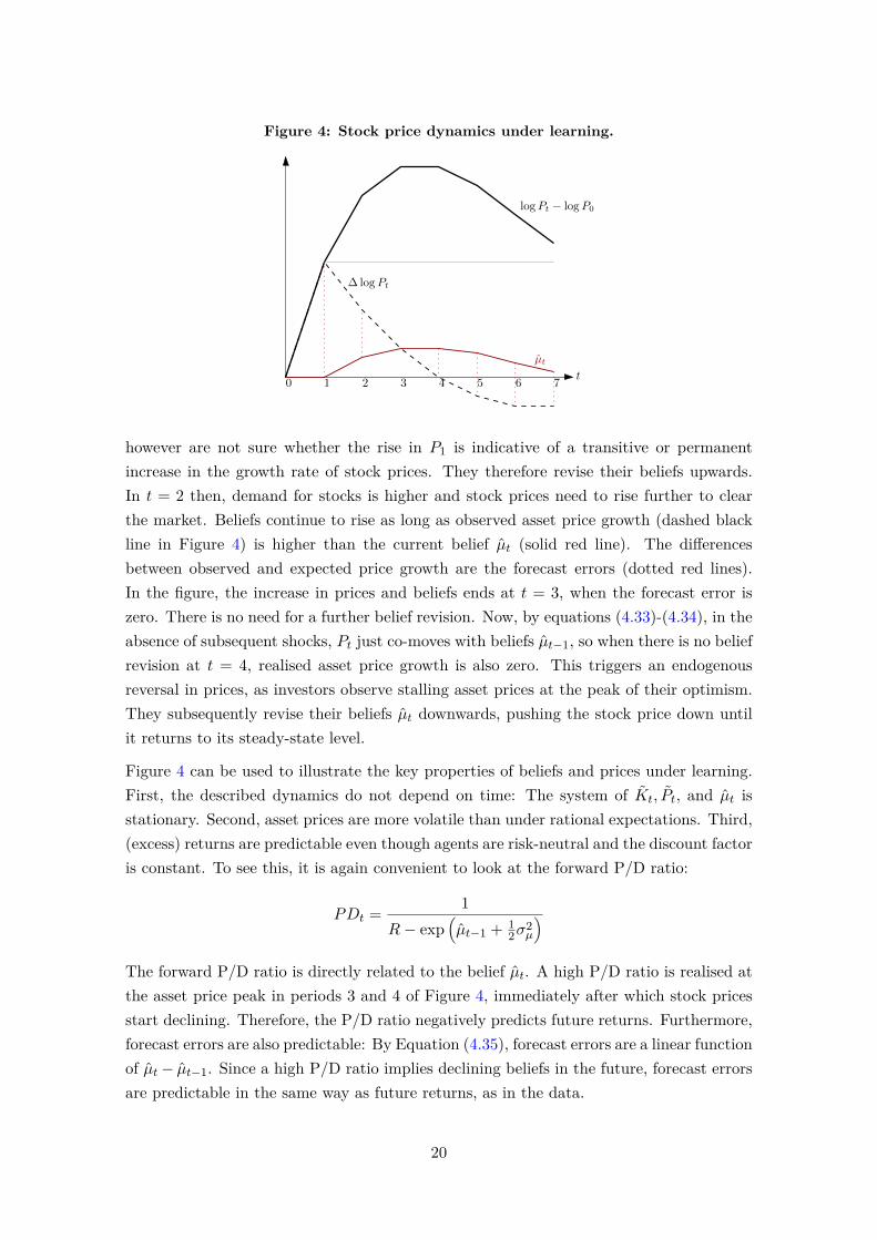
Figure 4: Stock price dynamics under learning.
t
logPt − logP0
∆ logPt
µt
0 1 2 3 4 5 6 7
however are not sure whether the rise in P1 is indicative of a transitive or permanentincrease in the growth rate of stock prices. They therefore revise their beliefs upwards.In t = 2 then, demand for stocks is higher and stock prices need to rise further to clearthe market. Beliefs continue to rise as long as observed asset price growth (dashed blackline in Figure 4) is higher than the current belief µt (solid red line). The differencesbetween observed and expected price growth are the forecast errors (dotted red lines).In the figure, the increase in prices and beliefs ends at t = 3, when the forecast error iszero. There is no need for a further belief revision. Now, by equations (4.33)-(4.34), in theabsence of subsequent shocks, Pt just co-moves with beliefs µt−1, so when there is no beliefrevision at t = 4, realised asset price growth is also zero. This triggers an endogenousreversal in prices, as investors observe stalling asset prices at the peak of their optimism.They subsequently revise their beliefs µt downwards, pushing the stock price down untilit returns to its steady-state level.
Figure 4 can be used to illustrate the key properties of beliefs and prices under learning.First, the described dynamics do not depend on time: The system of Kt, Pt, and µt isstationary. Second, asset prices are more volatile than under rational expectations. Third,(excess) returns are predictable even though agents are risk-neutral and the discount factoris constant. To see this, it is again convenient to look at the forward P/D ratio:
PDt = 1R− exp
(µt−1 + 1
2σ2µ
)The forward P/D ratio is directly related to the belief µt. A high P/D ratio is realised atthe asset price peak in periods 3 and 4 of Figure 4, immediately after which stock pricesstart declining. Therefore, the P/D ratio negatively predicts future returns. Furthermore,forecast errors are also predictable: By Equation (4.35), forecast errors are a linear functionof µt− µt−1. Since a high P/D ratio implies declining beliefs in the future, forecast errorsare predictable in the same way as future returns, as in the data.
20

Figure 5: Endogenous response of dividends.
Kt
1−ξξ Kt
D(Kt,Kt)R−exp(µt)
µ0
µ1
µ2
K∗
P0, P1
P2
P3
Pt
(a) Amplification.
Kt
1−ξξ Kt
D(Kt,Kt)R−exp(µt−1)
µ0
µ1
µ2
K∗
P0, P1
P2
P3
Pt
(b) Dampening.
The aforementioned asset pricing implications are present even when dividends are com-pletely exogenous, as in Adam et al. (2013). But the model considered here also containsa link between asset prices, output and dividends. The effective capital stock Kt is dir-ectly related to equity valuations Pt through Equation (4.34). Thus, the fluctuations in thestock market translate into corresponding fluctuations in investment, the capital stock andhence output. Thus, the presence of financial frictions in combination with learning leadsto amplification of productivity shock, whereby under rational expectations amplificationwas zero.
It is also possible that this amplification mechanism is further enhanced by positive feed-back from capital to expected dividends. This additional feedback, however, depends onthe slope of the function D. As demonstrated above, the expected dividend D
(kt, Kt
)is
increasing in the firm’s capital choice kt, but decreasing in the aggregate capital stock Kt.In the equilibrium (kt = Kt) it is increasing if financial frictions are sufficiently severe.This case is depicted in Panel (a) of Figure 5. When the degree of financial frictions ishigh, the credit constraint line is steep. Assume that the initial equilibrium in period0 is at P0 and µ0. Now consider the effect of a positive productivity shock in period 1as before. The immediate effect will be a proportionate rise in stock prices and capitalwhich leaves P1 and K1 unchanged, but raises beliefs from µ0 to µ1. This leads to higherstock prices at t = 2 and allows the firm to invest more and increase its expected profitsD(K2, K2
). But this adds further to the rise in realised stock prices, further relaxing the
borrowing constraint and increasing next period’s beliefs. Stock prices, beliefs, investment,and output all rise by more compared to a situation in which D is constant.14
14To my knowledge, this paper is the first to establish a positive feedback from fundamentals to beliefsunder learning. Adam et al. (2012) also model economies with endogenous fundamentals. Their learningspecification is similar, but the “dividend” in their asset pricing equation is simply the marginal utility ofhousing which is strictly decreasing in the level of the housing stock. Their model dynamics are thereforealways as in case (b) described above.
21

However, this additional amplification channel only works when ξ is sufficiently low. InPanel (b), ξ is large and the firm is operating in the downward-sloping bit of the profitcurve D. A relaxation of the borrowing constraint due to a rise in µ still allows thefirm to invest and produce more, but dividends fall in equilibrium. This is due to thegeneral equilibrium forces mentioned earlier: The marginal product of capital has to fallin equilibrium, which in practice derives from an increase in real wages, effectively reducingthe firm’s profits. In this situation, the endogenous response of dividends dampens ratherthan amplifies the dynamics of investment and asset prices.
This can also be seen algebraically. Under rational expectations, the derivative of log stockprices with respect to the productivity shock is simply d logPt/dεt−s = 1 for all t, s ≥ 0.With learning, the corresponding expression contains additional terms:
d logPtdεt−s
= 1 + 11− εD
(Kt
) eµt−1
R− eµt−1
dµtdεt−s
(4.36)
where εD(Kt
)= dD
dKKD
is the elasticity of expected dividends with respect to the capitalstock. Learning adds a product of three terms. The last term is the effect of the pro-ductivity shock on subjective beliefs. The second term is the effect of beliefs on stockprices. Small variations in beliefs µt cause large fluctuations in stock prices because thedenominator
(R− eµt−1
)is close to zero. The first term captures the general equilibrium
effects mentioned earlier: when dividends rise after a relaxation of credit constraints, εdkis positive and the term is greater than one, leading to additional amplification, and todampening when εdk is negative.
It can also be shown that the learning dynamics vanish as the economy approaches theunconstrained first-best:
d logPtdεt−s
ξ→1−→ 1
In other words, amplification rests on the interaction between learning and financial fric-tions, not on either of them separately. Intuitively, as financial frictions disappear, theeconomy moves into a region where the general equilibrium effects become so strong thatany potential rise in beliefs or asset prices is countered by a fall in expected dividends.
In sum, the learning equilibrium can qualitatively account for a number of asset pricingfacts and for the predictability of forecast errors. At the same time, the larger endogenousasset price volatility induces corresponding fluctuations in the slackness of the firm’s bor-rowing constraint. The presence of financial frictions thus magnifies productivity shocks,while there is no amplification under rational expectations. When financial frictions aresufficiently severe, a two-sided positive feedback loop emerges between beliefs, asset pricesand firm profits, which further amplifies the dynamics. The presence of positive feedbackfrom assets prices to profits depends on the relative strength of general equilibrium forces,which in the model in this section operate through the real wage.
I now turn to the development of a richer model that embeds the same mechanism, but
22

can also be taken to the data to study its quantitative implications.
5 Full model for quantitative analysis
This section embeds the mechanism discussed previously into a New-Keynesian businesscycle model with a financial accelerator. Compared to the simple model in the previoussection, there are a number of new elements. First, capital no longer has to be financedentirely out of debt. Instead, I allow for endogenous fluctuations in net worth. To preventfirms from saving until they become unconstrained, I impose exogenous entry and exit,as in Bernanke, Gertler and Gilchrist (1999). Second, I provide a microfoundation of theborrowing constraint by means of a limited commitment problem. Third, I add severalstandard business cycle frictions: nominal rigidities, which enables me to introduce mon-etary policy and later on analyse its effects on welfare under learning; and investmentadjustment costs, which allow for a better fit of the model.
5.1 Model setup
The economy is closed and operates in discrete time. There are a number of differentagents:
1. Intermediate goods producers (or simply firms) are at the heart of the model. Theycombine capital and and differentiated labour to produce a homogeneous intermedi-ate good. They are financially constrained and borrow funds from households.
2. Firm owners only consume differentiated final goods. They trade shares in interme-diate goods producers and receive dividend payments.
3. Households consume differentiated final goods and supply homogeneous labour tolabour agencies. They lend funds to intermediate goods producers.
4. Labour agencies transform homogeneous household labour into differentiated labourservices, which they sell to intermediate goods producers. They are owned by house-holds.
5. Final good producers transform intermediate goods into differentiated final goods.They are owned by households.
6. Capital goods producers produce new capital goods from final consumption goodssubject to an investment adjustment cost.
7. The fiscal authority sets certain tax rates to offset steady-state distortions frommonopolistic competition.
8. The central bank sets nominal interest rates.
23

Since most elements of the model are standard, I focus on the financially constrainedfirms, firm owners, households and the central bank. Additional details are provided inAppendix A.
5.1.1 Households
A representative household with time-separable preferences maximises utility as follows:
max(Ct,Lt,Bjt,Bgt )∞t=0
EP0∞∑t=0
βtu (Ct, Lt)
s.t. Ct = wtLt +Bgt − (1 + it−1) pt−1
ptBgt−1 +
ˆ 1
0(Bjt −Rjt−1Bjt−1) dj + Πt
The utility function u satisfies standard concavity and Inada conditions and β ∈ (0, 1).Further, wt is the real wage received by the household and Lt is the amount of laboursupplied. Bg
t are real quantities of nominal one-period government bonds (in zero netsupply) that pay a nominal interest rate it and pt is the price level, defined below. House-holds also lend funds Bjt to intermediate goods producers indexed by j ∈ [0, 1] at the realinterest rate Rjt. These loans are the outcome of a contracting problem described later on.Πt represents lump-sum profits and taxes. Finally, consumption Ct is itself a compositeutility flow from of a variety of differentiated goods that takes the familiar CES form:
Ct = maxCit
(ˆ 1
0(Cit)
σ−1σ di
) σσ−1
s.t. ptCt =ˆ 1
0pitCitdi
As usual, the price index pt of composite consumption consistent with utility maximisationand the demand function for good i is given by
pt =(ˆ 1
0(pit)1−σ di
) 11−σ
; Cit =(pitpt
)−σCt. (5.1)
Consequently, the inflation rate is given by πt = pt/pt−1. The first order conditions of thehousehold are also standard and given by
wt = −uLtuCt
(5.2)
1 = EPt βuCt+1uCt
1 + itπt
. (5.3)
We can define the stochastic discount factor of the households as Λt = βuCt+1/uCt.
24
5.1.2 Central bank
Like most of the New-Keynesian literature, the model is cashless, with the central bankaffecting allocations in the presence of nominal rigidities by setting the nominal interestrate. In the baseline version of the model, I assume that the central bank conductsmonetary policy through the use of a Taylor-type interest rate rule:
it = ρiit−1 + (1− ρi) (1/β + πt + φπ (πt − π∗t )) (5.4)
where π∗t is the central bank’s (time-varying) inflation target, ρi is the degree of interestrate smoothing and φπ > 1.
5.1.3 Intermediate good producers (firms)
The production of intermediate goods is carried out by a continuum of firms, indexedj ∈ [0, 1]. Firm j enters period t with capital Kjt−1 and a stock of debt Bjt−1 which needsto be repaid at the gross real interest rate Rjt−1. First, capital is combined with a labourindex Ljt to produce output
Yjt = (Kjt−1)α (AtLjt)1−α , (5.5)
where At is aggregate productivity. The labour index is a CES combination of differenti-ated labour services parallel to the differentiated final goods bought by the household:
Ljt = maxLjht
(ˆ 1
0(Ljht)
σw−1σw dh
) σwσw−1
(5.6)
s.t. wtptLjt =ˆ 1
0WjhtLjhtdh (5.7)
The firm’s problem can then be treated as if the labour index was acquired in a competitivemarket at the real wage index wt.15 Output is sold competitively to final good producersat price qt. During production, the capital stock depreciates at rate δ. This depreciatedcapital can be traded by the firm at the price Qt.
At this point, the net worth of the firm is the difference between the value of its assetsand its outstanding debt:
Njt = qtYjt − wtLjt +Qt (1− δ)Kjt−1 −Rjt−1Bjt−1 (5.8)
I assume that the firm exits with a probability γ. This probability is exogenous andindependent across time and firms. As in Bernanke et al. (1999), exit prevents firms frombecoming financially unconstrained. If a firm does not exit, it needs to pay out a fraction
15This real wage index does not necessarily equal the wage wt received by households due to wagedispersion.
25
ζ of its earnings as dividends, where earnings are given by Ejt = Njt−QtKjt−1 +Bjt−1.16
If it exits, it must pay out its entire net worth as dividends. It is subsequently replacedby a new firm which receives the index j. I assume that this new firm gets endowed witha fixed number of shares, normalised to one, and is able to raise an initial amount of networth. This amount equals ω (Nt − ζEt) where ω ∈ (0, 1) and Nt and Et are aggregatenet worth and earnings, respectively.
The net worth of firm j after equity changes, entry and exit is given by
Njt =
Njt − ζEjt for continuing firms,
ω (Nt − ζEt) for new firms.
This firm then decides on the new stock of debt Bjt and the new capital stock Kjt. Itsbalance sheet must satisfy:
QtKjt = Bjt + Ntj (5.9)
where the price of capital Qt can vary in the presence of adjustment costs.
Firms maximise the present discounted value of their dividend payments using the discountfactor of their owners. In doing so, they face financial constraints. Before describing theseconstraints though, I first turn to the description of the firms’ owners.
5.1.4 Firm owners
Firm owners differ from households in their capacity to own intermediate firms. Therepresentative firm owner is risk-neutral and discounts future income at the rate β =βG−θ < β, with G being the growth rate of consumption in the non-stochastic steadystate. He can buy shares in firms indexed by j ∈ [0, 1]. As described above, when a firmexits it pays out its net worth Njt as dividends, and is replaced by a new firm which raisesequity ω (Nt − ζEt). Let the set of exiting firms in each period t be denoted by Γt ⊂ [0, 1].Then, the firm owner’s utility maximisation problem is given by:
max(Cft ,S
jt
)∞t=0
EP0∞∑t=0
βtCft
16The optimal dividend policy in this model would be to never pay dividends until exit. In this case,aggregate dividends would be proportional to aggregate net worth. This implies a dividend process that isnot nearly as volatile as in the data, and thus makes it impossible to obtain good asset pricing propertieseven under learning. Imposing that firms need to pay out a fraction of their earnings greatly improves thequantitative fit of the model.
26

s.t. Cft +ˆ 1
0SjtPjtdj =
ˆj /∈Γt
Sjt−1 (Pjt +Djt) dj (5.10)
+ˆj∈Γt
[Sjt−1Djt − ω (Nt − ζEt) + Pjt] dj (5.11)
Sjt ∈[0, S
](5.12)
for some S > 1. Here, firm owners’ consumption Cft is the same aggregator of differentiatedfinal goods as for households.
The first term on the right hand side of the budget constraint deals with continuing firmsand is standard: Each share in firm j pays dividends Djt and continues to trade, at pricePjt. The second term deals with firm entry and exit. If the household owns a share inthe exiting firm j, he receives a terminal dividend. The firm is then delisted in the stockmarket, and so Sjt−1Pjt does not appear. At the same time, a new firm j appears whichis able to raise a limited amount of equity ω (Nt − ζEt) from the firm owner in exchangefor a unit amount of shares that can be traded at price Pjt. In addition, upper andlower bounds on traded stock holdings are introduced to make firm owners’ demand forstocks finite under arbitrary beliefs, as in the stylised model of the previous section. Inequilibrium, they are never binding.
The first order conditions of the firm owner are
Sjt
= 0 if Pjt > βEPt
[Djt+1 + Pjt+11{j /∈Γt+1}
]∈[0, S
]if Pjt = βEPt
[Djt+1 + Pjt+11{j /∈Γt+1}
]= S if Pjt < βEPt
[Djt+1 + Pjt+11{j /∈Γt+1}
] (5.13)
5.1.5 Borrowing constraint
In choosing their debt holdings, firms are subject to a borrowing constraint. The constraintis the solution to a particular limited commitment problem in which the outside optionfor the lender in the event of default depends on equity valuations.
Each period, lenders (households) and borrowers (firms) meet to decide on the lending offunds. Pairings are anonymous to rule out repeated interactions. The incompleteness ofcontracts imposed is that repayment of loans cannot be made contingent. Only the sizeBjt and the interest rate Rjt of the loan can be contracted in period t. Both the lender(a household) and the firm have to agree on a contract (Bjt, Rjt). Moreover, there islimited commitment in the sense that at the end of the period, but before the realisationof next period’s shocks, firm j can always choose to enter a state of default. In this case,the value of the debt repayment must be renegotiated. If the negotiations are successful,then wealth is effectively shifted from creditors to debtors. The outside option of thisrenegotiation process is the seizure of the firm by the lender, in which case the currentfirm owners receive zero.
27

The lender, a household, does not have the ability to run the firm though. The usualassumption in the literature is that she has to liquidate the firm’s asset in this case. Inthis model, the lender can always liquidate as well. In this case, all debt and a fraction 1−ξof the firm’s capital is destroyed. The remaining capital can be sold in the next period,resulting in a total recovery value of ξQt+1Kjt. On top of this, with some probability x(independent across time and firms), the lender gets the opportunity to “restructure” thefirm. Restructuring means that, similar to Chapter 11 bankruptcy proceedings, the firmgets partial debt relief but remains operational. I assume that the lender has to sell thefirm to another firm owner, retaining a fraction ξ of the initial debt. It will turn out inequilibrium that the recovery value in this case is just ξ (Pjt +Bjt) and that lenders alwaysprefer restructuring to liquidation. The debt contract then takes the form of a leverageconstraint in which total firm value is a weighted average of liquidation and market value:
Bjt ≤ ξ
xEPt Λt+1Qt+1ξKjt︸ ︷︷ ︸liquidation value
+ (1− x) (Pjt +Bjt)︸ ︷︷ ︸market value
(5.14)
5.1.6 Further model elements and market clearing
Final good producers, indexed by i ∈ [0, 1], combine the homogeneous intermediate goodinto a differentiated final good using a one-for-one technology. Their revenue is sub-sidised by the government at the rate τ .17 Per-period profits of producer i are ΠY
it =(1 + τ) (pit/pt)Yit−qtYit. They are subject to a Calvo price setting friction: Every period,each final-good producer can change his price only with probability 1 − κ, independentacross time and producers. Similarly, labour agencies (indexed by h ∈ [0, 1]) combine thehomogeneous labour provided by households into differentiated labour goods which theysell on to intermediate good producers. labour agencies’ revenue is subsidised at the rateτw, the per-period profit of agency h is ΠL
ht = (1 + τ) (Wht/pt)Lht−wtLht and each agencycan change its nominal wage Wht only with probability 1− κw. The government collectssubsidies as lump sum taxes from households and runs a balanced budget each period.The government sets the subsidy rates such that under flexible prices, the markup overmarginal cost is zero in both the labour and output markets.
Capital goods producers produce new capital goods subject to standard investment ad-justment costs and have profits ΠI
t . Thus, the total amount of lump-sum payments Πt
received by the household is the sum of the profits of all final good producers, labouragencies and capital goods producers, minus the sum of all subsidies.
17This assumption is standard in the New-Keynesian literature. It eliminates distortions from monopol-istic competition where firms price above marginal cost. The only distortion is then due to sticky prices,which simplifies the solution by perturbation methods.
28

Finally, the exogenous stochastic processes are productivity and the inflation target shock:
logAt = t (1− ρ) logG+ ρ (logAt−1 + logG) + log εAt (5.15)
π∗t = ρππ∗t−1 + log επt (5.16)
εAt ∼ N(0, σ2
A
)(5.17)
επt ∼ N(0, σ2
π
)(5.18)
Market clearing needs to take into account the distortions from price and wage dispersion.All market clearing conditions are listed in Appendix A.
5.2 Rational expectations equilibrium
I first describe the equilibrium under rational expectations. Equilibrium is a set ofstochastic processes for prices and allocations, a set of strategies in the limited com-mitment game, and an expectation measure P such that the following holds for all statesand time periods: Markets clear; allocations solve the optimisation programmes of allagents given prices and expectations P; the strategies in the limited commitment gameare a subgame-perfect Nash equilibrium for all lender-borrower pairs; and the measure Pcoincides with the actual probability measure induced by the equilibrium.
Under appropriate parameter restrictions, there exists a rational expectations equilibriumcharacterised by the following properties (proofs and characterisation of the restrictionsare relegated to Appendix B):
1. All firms choose the same capital-labour ratio Kjt/Ljt. This allows one to define anaggregate production function and an internal rate of return on capital:
Yt = αKαt−1
(AtLt
)1−α(5.19)
Rkt = qtαYtKt−1
+Qt (1− δ)Kt−1 (5.20)
2. The expected return on capital is higher than the internal return on debt: EtRkt+1 >
Rjt.
3. At any time t, the stock market valuation Pjt of a firm j is proportional to its networth after entry and exit Njt. This permits one to write an aggregate stock marketindex as
Pt =ˆ 1
0Pjt = βEt
[Dt+1 + 1− γ
1− γ + γωPt+1
]. (5.21)
The “correction” term in the continuation value Pt+1 can be understood as follows.The stock market index Pt is the value of all currently existing firms, not includingfirms that are not yet born. In t + 1, a fraction γ of firms exit and pay dividends
29

γNt. The remaining firms are left with net worth (1− γ)Nt+1 and pay dividends(1− γ) ζEt and , but a mass γ of new firms also enters, each endowed with initialnet worth ω (Nt − ζEt).
4. Borrowers never default on the equilibrium path and borrow at the risk-free rate
Rjt = Rt = (EtβuCt+1/uCt)−1 . (5.22)
The lender only accepts debt payments up to a certain limit Bjt. The firm alwaysexhausts this limit, Bjt = Bjt, which is proportional to the firm’s net worth Njt. Ifthe firm defaulted and the lender seized the firm, she would always prefer restructur-ing to liquidation. Intuitively, this is because capital is more valuable inside the firmthan outside of it. Because acquiring capital is difficult due to financial frictions,firm owners will always pay the lender a higher price for a restructured, operationalfirm than for its capital stock alone.
5. As a consequence of the previous properties of the equilibrium, all firms can beaggregated. Aggregate debt, capital, and net worth are sufficient to describe theintermediate goods sector and evolve as
Nt = RktKt−1 −Rt−1Bt−1 (5.23)
QtKt = (1− γ + γω) ((1− ζ)Nt + ζ (Bt−1 −QtKt−1)) +Bt (5.24)
Bt = xEtΛt+1Qt+1ξKt + (1− x) ξ (Pt +Bt) . (5.25)
I solve for a second-order approximation of this rational expectations equilibrium aroundits non-stochastic steady state.
5.3 Learning equilibrium
I introduce learning about stock market valuations as in the simple model of Section 4.One slight complication is now that there is a continuum of firms to be priced in themarket. In this respect, I retain the belief that the stock price of an individual firm isproportional to firm net worth, as is the case under rational expectations. As such, underP,
Pjt = Njt
NtPt. (5.26)
But while investors know how to price individual stocks by observing the valuation of themarket, they are uncertain about the evolution of the market itself. As in the simple modelof the previous section, I impose the same beliefs about aggregate stock prices as in the lastsection along with the other assumptions (equations (4.25)-(4.28)), including expectationson other variables that are conditionally consistent with outcomes on the equilibriumpath: For any variable xt, any future date t + τ , and any sequence of stock prices and
30
fundamentals (denoted by ut) which is on the equilibrium path, agents’ conditional beliefscoincide with equilibrium outcomes: EPt [xt+τ | ut, Pt, . . . , ut+τ , Pt+τ ] = xt+τ almost surely.
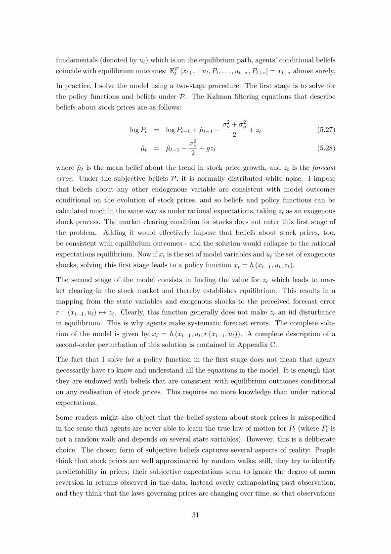
In practice, I solve the model using a two-stage procedure. The first stage is to solve forthe policy functions and beliefs under P. The Kalman filtering equations that describebeliefs about stock prices are as follows:
logPt = logPt−1 + µt−1 −σ2ν + σ2
η
2 + zt (5.27)
µt = µt−1 −σ2ν
2 + gzt (5.28)
where µt is the mean belief about the trend in stock price growth, and zt is the forecasterror. Under the subjective beliefs P, it is normally distributed white noise. I imposethat beliefs about any other endogenous variable are consistent with model outcomesconditional on the evolution of stock prices, and so beliefs and policy functions can becalculated much in the same way as under rational expectations, taking zt as an exogenousshock process. The market clearing condition for stocks does not enter this first stage ofthe problem. Adding it would effectively impose that beliefs about stock prices, too,be consistent with equilibrium outcomes - and the solution would collapse to the rationalexpectations equilibrium. Now if xt is the set of model variables and ut the set of exogenousshocks, solving this first stage leads to a policy function xt = h (xt−1, ut, zt).
The second stage of the model consists in finding the value for zt which leads to mar-ket clearing in the stock market and thereby establishes equilibrium. This results in amapping from the state variables and exogenous shocks to the perceived forecast errorr : (xt−1, ut) 7→ zt. Clearly, this function generally does not make zt an iid disturbancein equilibrium. This is why agents make systematic forecast errors. The complete solu-tion of the model is given by xt = h (xt−1, ut, r (xt−1, ut)). A complete description of asecond-order perturbation of this solution is contained in Appendix C.
The fact that I solve for a policy function in the first stage does not mean that agentsnecessarily have to know and understand all the equations in the model. It is enough thatthey are endowed with beliefs that are consistent with equilibrium outcomes conditionalon any realisation of stock prices. This requires no more knowledge than under rationalexpectations.
Some readers might also object that the belief system about stock prices is misspecifiedin the sense that agents are never able to learn the true law of motion for Pt (where Pt isnot a random walk and depends on several state variables). However, this is a deliberatechoice. The chosen form of subjective beliefs captures several aspects of reality: Peoplethink that stock prices are well approximated by random walks; still, they try to identifypredictability in prices; their subjective expectations seem to ignore the degree of meanreversion in returns observed in the data, instead overly extrapolating past observation;and they think that the laws governing prices are changing over time, so that observations
31

from the distant past are only of limited usefulness in predicting the future.
5.4 Frictionless benchmark
Because my aim is to gauge the importance of financial frictions for business cycle analysis,I will also use a benchmark model without financial frictions to which the model can becompared to. This benchmark model will be identical to the rational expectations modelabove, except that intermediate firms are now owned by households, and face no frictionsin accessing external finance.
5.5 Choice of parameters
I partition the set of parameters into two groups. The first set of parameters is calibratedto first moments, and the second set is estimated by simulated method of moments.
5.5.1 Calibration
The capital share in production is set to α = .33, implying a labour share in output oftwo thirds. The depreciation rate δ = .025 corresponds to 10% annual depreciation. Thenon-stochastic trend productivity growth rate G is set to its post-war average of 1.64%annually. The persistence of the temporary component of productivity is set to .95.
The discount factor of the household is set such that the steady-state interest rate matchesthe average annual real return on Treasury bills of 2%, implying a discount factorβ = .9991.The firm owners’ discount factor is set such that in the non-stochastic steady state, bondsand stocks have the same return (β = .995). The elasticity of substitution betweenvarieties of the final consumption good, as well as that between varieties of labour usedin production, is set to σ = σw = 4. The Frisch elasticity of labour supply is set to three,implying φ = .33.
The strength of monetary policy reaction to inflation is set to φπ = 1.5, while the degreeof nominal rate smoothing is set to ρi = 0.5. The inflation target is set to π∗ = 0. Thepersistence of the inflation target is set to ρπ = .99.
Four parameters describe the structure of financial constraints: x, the probability of re-structuring after default; ξ, the tightness of the borrowing constraint; ω, the equity receivedby new firms relative to average equity; and γ, the rate of firm exit and entry. I calibratethe restructuring rate x to equal 9.3%. This is the fraction of US business bankruptcyfilings in 2006 which filed for Chapter 11 instead of Chapter 7, and which subsequentlyemerged from bankruptcy with an approved restructuring plan. I have to restrict myselfto 2006 because it is the only year for which this number can be constructed. Public bank-ruptcy data shows that the fraction of Chapter 11 cases as opposed to Chapter 7 casesfluctuates around 28%, and several papers analysing sub-samples of Chapter 11 filings
32
arrive at confirmation rates between 29% and 64%, which suggests that the 2006 numberis reasonable (a sensitivity check is included in Section 6.5).18 The remaining three para-meters are chosen such that the non-stochastic steady state of the model jointly matchesthe US average investment share in output of 20%, average debt-to-equity ratio of 1:1(as recorded in the Fed Flow of Funds), and average quarterly P/D ratio of 139 (takenfrom the S&P500). The parameter values thus are γ = 0.010, ξ = 0.38, and ω = 0.55.Intuitively, a larger value of ξ relaxes the borrowing constraint, leading to higher leverage.A larger value of ω means that new firms enter with more equity, increasing aggregatenet worth and capital. Since returns on capital are diminishing, this raises the investmentshare in output. A higher rate of exit γ makes firms shorter-lived, reducing the firm’svalue relative to its current dividend payments, thereby lowering the P/D ratio.
5.5.2 Estimation
The remaining parameters are the standard deviations of the technology and monetaryshocks (σA, σπ), the size of investment adjustment costs (ψ), the degree of nominal priceand wage rigidities (κ, κw), the fraction of dividends paid out as earnings by continuingfirms (ζ), and the learning gain (g). Since my goal is to see how well the model cando in terms of matching both business cycle and asset pricing facts, I estimate theseparameters to minimise the distance to a set of second moments pertaining to both. I usethe variances of the nominal interest rate, the inflation rate, real output, consumption,investment, employment, as well as real dividend payments and stock prices in the data.19
The set of estimated parameters θ solves
minϑ∈A
(m (θ)− m)′W (m (θ)− m)′
where m (θ) are moments obtained from model simulation paths with 50,000 periods, mare the estimated moments in the data, and W is a weighting matrix.20 I also impose thatθ has to lie in a subset A of the parameter space which rules out deterministic oscillationsof impulse response functions.21 Parameters outside this region would fit the moments wellbut can be ruled out from prior knowledge about the shape of impulse responses. Table
18Data on bankruptcies by chapter are available at http://www.uscourts.gov/Statistics/BankruptcyStatistics.aspx. Data on Chapter 11 outcomes are analysed in various samples by Flynnand Crewson (2009), Warren and Westbrook (2009), Lawton (2012), and Altman (2014).
19All variables are at quarterly frequency and HP-detrended. I use CPI inflation as the inflation measureand the Federal Funds rate as the nominal interest rate. Employment is total non-farm payroll employment.Consumption is the sum of services and non-durable private consumption. Investment is the sum ofprivate non-residential fixed investment and durable consumption. Output is the sum of consumptionand investment. Dividend payments are the four-quarter moving average of S&P 500 dividends and stockprices is the S&P500 index.
20I choose W = diag(Σ)−1 where Σ is the covariance matrix of the data moments, estimated using a
Newey-West kernel with optimal lag order. This choice ofW leads to a consistent (albeit not fully efficient)estimator that places more weight on moments which are more precisely estimated in the data.
21To be precise, θ /∈ A if there exists an impulse response of stock prices with positive peak value alsohaving a negative value of more than 20% of the peak value.
33

Table 3: Estimated parameters.
parameter value s.e.
σA 0.00685 (0.00150)
σπ 8.94·10−4 (2.55·10−4)
ψ 10.6 ( 3.10)
κ 0.809 ( 0.123)
κw 0.943 ( 0.0233)
ζ 0.8209 ( 0.0197)
g 0.00460 (9.76·10−4)
Parameters as estimated by simulated method of moments. Asymptotic standard errors in parentheses.
3 summarises the results of the estimation. It selects a rather high degree of adjustmentcosts (although imprecisely estimated) and of nominal rigidities. The fraction of earningspaid out as dividends is fitted to more than 80%, higher than the actual historical averagefor the S&P500 at about 50%. This suggests that my assumption about the behaviourof dividends is overly simplistic. This is a commonly encountered problem (Covas andDen Haan, 2012) which I have to leave for future research. Finally, a low estimate for thelearning gain g implies that agents believe the predictability of stock prices to be small.
6 Results
6.1 Business cycle and asset price moments
To get a better understanding of the quantitative properties of the model, Table 4 reviewskey business cycle moments as well as the statistics describing stock price volatility andreturn predictability across model specifications. The moments for the estimated learningmodel are in Column (1), while Columns (2) and (3) contain the corresponding momentsfor the model under rational expectations and the frictionless benchmark. Here, theparameters are held constant at the same values as for the learning model. By natureof the estimation, the learning model has the best fit across Columns (1) to (3). Thecomparison serves to single out the contribution of learning and financial frictions to thefit. In Column (4), I also let the rational expectations version of the model compete withthe learning model: I re-estimate the same model parameters (σA, σπ, ψ, κ, κw) using thesame objective function as before, minimising the distance between the moments in thedata and in the model.22
22The re-estimated parameters are σA = .00664, σπ = .00112, ψ = .0557, ζ = .446, κ = .797 andκw = .915. Standard errors around the estimates are large.
34

Table 4: Comparing moments in the data and across model specifications.
(1) (2) (3) (4)
moment data learning RE fric.less RE re-estimated
output σhp (Yt) 1.43% 1.41% .76% .55% 1.39%
consumption σhp (Ct) /σhp (Yt) 0.60 .64 1.11 1.43 .63
investment σhp (It) /σhp (Yt) 2.90 3.11 .55 .34 3.02
employment σhp (Lt) /σhp (Yt) 1.13 1.21 1.00 1.02 1.18
inflation σhp (πt) /σhp (Yt) .19 .22 .36 .47 .22
nominal rate σhp (it) /σhp (Yt) .20 .20 .32 .43 .19
dividends σhp (Dt) /σhp (Yt) 2.99 3.07 2.36 - 1.11
excess σhp (Pt) /σhp (Dt) 2.63 1.81 .21 - .18
volatility σ(PtDt
).408 .131 .037 - .037
σ(Rstockt,t+1
).335 .150 .011 - .010
return ρ(PtDt, Rstockt,t+4
)-.218 -.240 -.002 - .025
predictability ρ(PtDt, Rstockt,t+20
)-.439 -.646 .015 - .024
ρ(PtDt, Pt+4Dt+4
).907 .432 .758 - .832
Quarterly US data 1962Q1-2012Q4. πt is quarterly CPI inflation. it is the Federal Funds rate. Lt
is total non-farm payroll employment. Consumption Ct consists of of services and non-durable privateconsumption. Investment It consists of private non-residential fixed investment and durable consumption.Output Yt is the sum of consumption and investment. Dividends Dt are four-quarter moving averages ofS&P 500 dividends. The stock price index Pt is the S&P500.
The first row reports the standard deviation of detrended output. By this measure, outputfluctuations under learning are double the size of those under rational expectations; inother words, learning adds considerable endogenous amplification to the model. In fact,the standard deviations of shocks in Column (4) needed to generate the same amount ofoutput volatility are much larger.
The following rows report the relative volatilities of key macroeconomic time series. Thelearning model matches all of them well. Shutting down learning leads to a sharp drop inthe volatility of investment and a corresponding increase in the volatility of consumption.This is because the estimated learning model features a rather high level of investmentadjustment costs to match investment volatility. Without high adjustment costs, thelearning model would transform the high degree of observed asset price volatility into acounterfactually high degree of investment volatility, i.e. the amplification mechanismwould be too strong. When the amplification is shut down in Columns (2) and (3),investment becomes very smooth and as a flip side, consumption is prevented from beingsmoothed. Looking at inflation and interest rates, shutting down learning increases their
35

volatility relative to output, although this is mostly due to the decrease in output volatilityitself. The volatility of employment and dividends is not much affected. Finally, the re-estimated model in Column (4) is able to match all moments just as well as under learningwith the exception of dividends.
Big differences appear in the asset price statistics. The learning model is able to approachthe volatility of prices and returns to a degree which is impossible to achieve even inthe re-estimated RE model.23 The ability to generate realistic stock price volatility is ofcourse at the heart of the amplification mechanism, since stock market valuations enterfirms’ borrowing constraints. Moreover, returns are negatively predicted by the P/D ratio.At the one year horizon, the predictability is very similar to that found in the data. Atthe five-year horizon however, it is too high. This is also reflected in the fact that theP/D ratio decays too fast, as documented in the last row. In a sense, this is not reallysurprising: The learning model has only one parameter (the learning gain g) to matchall statistics pertaining to stock prices. In particular, it can be shown that a higher gainincreases volatility, but reduces persistence of prices. A richer belief specification couldpossibly achieve a better fit, but at the expense of introducing additional parameters.
6.2 Impulse response functions
Looking at impulse response functions reveals some of the workings of the amplificationmechanism at play. Figure 6 plots the impulse responses to a persistent productivity shock.Red solid lines represent the learning equilibrium, blue dashed lines represent the rationalexpectations version, and black thin lines represent the frictionless benchmark. Lookingat the response of output Yt, one can see quite clearly how the rational expectations ver-sion generates only a slightly amplified reaction to the shock compared to the frictionlessbenchmark. With learning, however, output rises by almost double the amount and theresponse is hump-shaped. Consumption Ct, and investment It also exhibit much strongerresponses, and employment Lt also rises considerably (without learning, it actually con-tracts). This amplification is due to the large rise in the stock prices Pt, even though thedegree of dependence of borrowing constraints on stock prices (measured by x) is less than10%. Under rational expectations, stock prices stay virtually flat, thus producing almostno amplification through the equity price channel. The behaviour of dividends Dt revealsthat initially, dividends fall, partly offsetting the rise of beliefs, but then overshoot theirrational expectations counterpart.
The feedback loop is also present after an interest rate shock. Figure 7 plots the response toa temporary reduction in the nominal interest rate. Again, all macroeconomic aggregatesrise substantially more under learning than under both rational expectations and thefrictionless benchmark. The monetary stimulus increases stock prices and thus relaxes
23In fact, it would be possible to obtain an even better fit of the asset pricing moments, but at theexpense of business cycle moments.
36
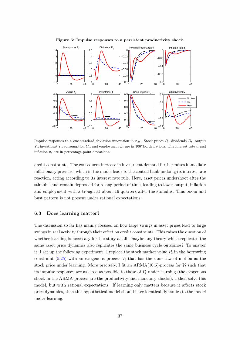
Figure 6: Impulse responses to a persistent productivity shock.
0 20 40−1
0
1
2
3
4Stock prices P
t
0 20 40−1
−0.5
0
0.5
1
1.5Dividends D
t
0 20 40−0.1
−0.08
−0.06
−0.04
−0.02
0Nominal interest rate i
t
0 20 40−0.2
−0.15
−0.1
−0.05
0Inflation rate π
t
0 20 40−0.2
0
0.2
0.4
0.6
0.8Output Y
t
0 20 40−0.5
0
0.5
1
1.5
2Investment I
t
0 20 400
0.1
0.2
0.3
0.4
0.5Consumption C
t
0 20 40−0.4
−0.2
0
0.2
0.4Employment L
t
fric.less
RE
learn
Impulse responses to a one-standard deviation innovation in εAt. Stock prices Pt, dividends Dt, outputYt, investment It, consumption Ct, and employment Lt are in 100*log deviations. The interest rate it andinflation πt are in percentage-point deviations.
credit constraints. The consequent increase in investment demand further raises immediateinflationary pressure, which in the model leads to the central bank undoing its interest ratereaction, acting according to its interest rate rule. Here, asset prices undershoot after thestimulus and remain depressed for a long period of time, leading to lower output, inflationand employment with a trough at about 16 quarters after the stimulus. This boom andbust pattern is not present under rational expectations.
6.3 Does learning matter?
The discussion so far has mainly focused on how large swings in asset prices lead to largeswings in real activity through their effect on credit constraints. This raises the question ofwhether learning is necessary for the story at all - maybe any theory which replicates thesame asset price dynamics also replicates the same business cycle outcomes? To answerit, I set up the following experiment. I replace the stock market value Pt in the borrowingconstraint (5.25) with an exogenous process Vt that has the same law of motion as thestock price under learning. More precisely, I fit an ARMA(10,5)-process for Vt such thatits impulse responses are as close as possible to those of Pt under learning (the exogenousshock in the ARMA-process are the productivity and monetary shocks). I then solve thismodel, but with rational expectations. If learning only matters because it affects stockprice dynamics, then this hypothetical model should have identical dynamics to the modelunder learning.
37

Figure 7: Impulse responses to a monetary shock.
0 20 40−1
0
1
2
3
4Stock prices P
t
0 20 40−2
−1
0
1
2Dividends D
t
0 20 40−0.1
−0.05
0
0.05
0.1Nominal interest rate i
t
0 20 40−0.02
−0.01
0
0.01
0.02
0.03
0.04Inflation rate π
t
0 20 40−0.2
0
0.2
0.4
0.6Output Y
t
0 20 40−0.5
0
0.5
1
1.5
2Investment I
t
0 20 40−0.1
0
0.1
0.2
0.3Consumption C
t
0 20 40−0.2
0
0.2
0.4
0.6
0.8Employment L
t
fric.less
RE
learn
Impulse responses to a one-standard deviation innovation in εmt. Stock prices Vt, dividends Dt, outputYt, investment It, consumption Ct and employment Lt are in 100*log deviations. The interest rate it andinflation pit are in percentage point deviations.
Figure 8 shows that this is not the case. The ARMA-process fits stock prices well: Theimpulse response of Pt under learning and Vt in the counterfactual experiment are indistin-guishable. But after a positive productivity shock, output, investment and consumptionrise much more under learning, even though the counterfactual model has the same stockprice dynamics by construction. The reason is found in the fact that expectations matterbeyond stock prices: For interest rates equilibrating loan demand by firms and supply byhouseholds; for inflation and wages, set by forward-looking Calvo price and wage setters;and for the borrowing constraint (5.25) itself, since it depends on the expected liquidationvalue of capital EtQt+1. This last channel is in fact crucial for the additional amplification.Under learning, agents do not understand that the increase in stock prices is temporary. Byover-predicting the slackness of borrowing constraints, they also over-predict the amountof investment taking place in the future, and hence the future price of capital. Lenders,predicting a high value of the firm’s capital stock, are then willing to lend more to firmstoday. Thus, identical firm market value still leads to easier access to credit under learning.
This illustrates how expectations in financial markets, over and above their effect on assetprices, can have important effects on the real economy.
6.4 Relation to survey evidence on expectations
Agents in the learning equilibrium make systematic, predictable forecast errors. Thepatterns of predictability are testable model implications. As it turns out, they are sur-
38
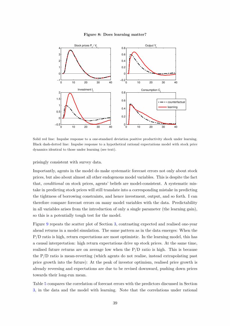
Figure 8: Does learning matter?
0 10 20 30 40−1
0
1
2
3
4Stock prices P
t / V
t
0 10 20 30 40−0.2
0
0.2
0.4
0.6
0.8Output Y
t
0 10 20 30 40−0.5
0
0.5
1
1.5
2Investment I
t
0 10 20 30 400
0.2
0.4
0.6
0.8Consumption C
t
counterfactual
learning
Solid red line: Impulse response to a one-standard deviation positive productivity shock under learning.Black dash-dotted line: Impulse response to a hypothetical rational expectations model with stock pricedynamics identical to those under learning (see text).
prisingly consistent with survey data.
Importantly, agents in the model do make systematic forecast errors not only about stockprices, but also about almost all other endogenous model variables. This is despite the factthat, conditional on stock prices, agents’ beliefs are model-consistent. A systematic mis-take in predicting stock prices will still translate into a corresponding mistake in predictingthe tightness of borrowing constraints, and hence investment, output, and so forth. I cantherefore compare forecast errors on many model variables with the data. Predictabilityin all variables arises from the introduction of only a single parameter (the learning gain),so this is a potentially tough test for the model.
Figure 9 repeats the scatter plot of Section 3, contrasting expected and realised one-yearahead returns in a model simulation. The same pattern as in the data emerges: When theP/D ratio is high, return expectations are most optimistic. In the learning model, this hasa causal interpretation: high return expectations drive up stock prices. At the same time,realised future returns are on average low when the P/D ratio is high. This is becausethe P/D ratio is mean-reverting (which agents do not realise, instead extrapolating pastprice growth into the future): At the peak of investor optimism, realised price growth isalready reversing and expectations are due to be revised downward, pushing down pricestowards their long-run mean.
Table 5 compares the correlation of forecast errors with the predictors discussed in Section3, in the data and the model with learning. Note that the correlations under rational
39

Figure 9: Return expectations and expected returns in a model simulation.−
.05
0.0
5.1
1y a
head fore
cast
3.4 3.5 3.6 3.7 3.8 3.9log P/D ratio
−.2
−.1
0.1
.2.3
1y a
head r
etu
rn
3.4 3.5 3.6 3.7 3.8 3.9log P/D ratio
Expected and realised nominal returns along a simulated path of model with learning. Simulation length200 periods. Theoretical correlation coefficient for expected returns ρ = .30, for realised returns ρ = −.11.
expectations need not be reported, as they are all zero by construction.
Column (1) reports predictability based on the P/D ratio. As already discussed, the cor-relation is negative, and it is even stronger in the data than in the model. The correlationis also negative for the other macroeconomic aggregates, again with a higher magnitudein the data. Column (2) repeats the exercise for the growth rate of the P/D ratio. Thismeasure positively predicts forecast errors: When the stock market is rising, people are onaverage not optimistic enough about returns and economic activity. This is because ex-pectations about asset prices (and hence lending conditions) adjust only slowly. Here, thedegree of correspondence with the data is striking. Only forecast errors on consumptionremain too weakly predictable in the model.
The model also does very well in terms of the Coibion and Gorodnichenko (2010) predict-ability statistic. As documented in Column (3), forecast errors on macro aggregates arepredictable by the direction of the forecast revision, again reflecting slow belief adjust-ment. This is also true in the model. For stock returns, the model predicts a negativecorrelation of return forecast errors with the revision, but the CFO survey does not allowfor the construction of a corresponding statistic.
Forecast error predictability is illustrated graphically in Figure 10. The solid red line is astandard impulse response function to a technology shock in the learning model. Considerthe following thought experiment. Suppose that at the time of the shock, the economy isin steady state and that no further shocks are realised. Under rational expectations, themean expectation about the future path of the economy at any point in time is then equalto the impulse response itself. Under learning, however, subjective expectations do notcoincide with the impulse response. The green dashed line of Figure 5 depicts the mean
40

Table 5: Forecast errors under learning and in the data.
(1) (2) (3)
forecast variable logPDt ∆ logPDt forecast revision
model data model data model data
Rstockt,t+4pt+4pt
-.22 -.44 .30 .06 -.19 n/a
Yt,t+3 -.10 -.21 .22 .22 .21 .29
It,t+3 -.14 -.20 .36 .25 .36 .31
Ct,t+3 -.04 -.19 .02 .21 .02 .23
ut,t+3 .10 .05 -.25 -.27 .15 .43
Data as in Table 2. Model correlations are exact theoretical correlations. Stock returns are nominalreturns. Unemployment in the model is taken to be ut = 1− Lt.
Figure 10: Actual versus expected impulse response.
5 10 150
1
2
3
Stock prices Pt
5 10 150
0.5
1
1.5
Investment It
5 10 150
0.1
0.2
0.3
0.4
0.5
0.6
Output Yt
Solid red line: Impulse response to a one-standard deviation positive productivity shock in Period 1. Greendashed line: mean subjective forecasts taken in Period 7. Blue dotted line: mean subjective forecasts takenin Period 3.
subjective forecast at the peak of the stock market. Agents do not foresee the decline inthe stock market, and instead extrapolate high stock price growth into the future. Becausestock market valuations matter for access to credit, agents also forecast loose borrowingconditions and are too optimistic about investment and output as well.24 The green dashedline (expectations) is above the red solid line (realisation) when the P/D ratio is high: Itnegatively predicts forecast errors. Next, the change in the P/D ratio predicts forecasterrors the other way around, which is illustrated with the blue dotted line. This is theforecast made at a time in which the P/D ratio is rising fast. In this situation, agentsunder-predict the size of the coming boom in the stock market and real activity. The bluedotted line is below the red solid line: Forecast errors are positive when P/D ratio growthis positive, too.
24Note that the forecasts for output and investment are still downward-sloping as agents are perfectlyaware of the mean reversion of productivity. Their long-run forecast has permanently higher stock prices,output and investment because of easier access to credit, while productivity remains at the steady-statelevel.
41

Figure 11: Parameter sensitivity.
0 0.05 0.1 0.15 0.2 0.25 0.30
2
4
6
8
σ(Y
)
0 0.05 0.1 0.15 0.2 0.25 0.30
5
10
15
20
25
σ(P
)
x
learning
RE
(a) Market value dependency x.
0 0.1 0.2 0.3 0.4 0.5 0.6 0.70
0.5
1
1.5
σ(Y
)
0 0.1 0.2 0.3 0.4 0.5 0.6 0.70
2
4
6
8
σ(P
)
ξ
learning
RE
(b) Recovery rate ξ.
0.8 0.82 0.84 0.86 0.88 0.9 0.92 0.94 0.96 0.980
2
4
6
σ(Y
)
0.8 0.82 0.84 0.86 0.88 0.9 0.92 0.94 0.96 0.980
10
20
30
σ(P
)
κw
learning
RE
(c) Wage rigidity κw.
4 6 8 10 12 140
1
2
3
4σ
(Y)
4 6 8 10 12 140
5
10
15
20
σ(P
)
ψ
learning
RE
(d) Investment adjustment cost ψ.
Theoretical standard deviations, unfiltered. Dashed black line indicates parameter value in the estimatedlearning model.
6.5 Sensitivity checks
The amount of endogenous amplification under learning relies on the dynamics of stockprices, and also on general equilibrium effects (as was already illustrated in the simplifiedmodel). To gain an idea of the sensitivity of the results, Figure 11 plots the volatility ofoutput and stock prices as a function of a set of influential parameters.
Panel (a) shows the role of the restructuring rate x which parametrises the dependencyof borrowing constraints on firm market value (as opposed to the liquidation value of itscapital). Not surprisingly, this parameter is key in driving amplification under learning.The point x = 0 is a special case. At this point, stock prices have no allocative role for theeconomy. Apart from stock prices then, the model dynamics under learning and rationalexpectations then coincide perfectly. Another special point is x = 1, where borrowingconstraints depend exclusively on stock prices. This was the case analysed in the simplemodel of Section 4. In the full model, this degree of stock price dependency leads to so
42

much amplification that the belief dynamics become explosive, and no stable equilibriumexists.25 Another remarkable fact is that the rational expectations solution barely dependson the parameter x. This might be one reason why the distinction between market andliquidation value has not featured prominently in the existing literature on firm creditfrictions.
Panel (b) shows the dependency on the average tightness of credit frictions ξ. Amplificationis hump-shaped with respect to this parameter. At ξ = 0, no collateral is pledgeableand firms cannot borrow at all. In this case, fluctuations in stock prices do not matterand learning does not introduce any amplification. On the other hand, as pledgeabilityincreases to its maximum value (beyond which a steady state with permanently bindingborrowing constraint does not exist), amplification also disappears. This mirrors theanalysis of the simplified model: when borrowing constraints relax, general equilibriumeffects in the form of wage and interest rate changes offset amplification.
Panels (c) and (d) document the importance of wage rigidity and investment adjustmentcosts, respectively. Wage rigidity helps to improve the fit of the model, but at the sametime it also helps amplification. When credit constraints relax, a larger degree of rigiditymitigates the negative general equilibrium effect on firm profits, raising internal net worthand stock prices. In contrast, adjustment costs dampen amplification since they makeinvestment more costly. The sensitivity to these parameters is much greater under learningthan under rational expectations.
7 Implications for monetary policy
In the model with learning, changes in subjective expectations in financial markets leadto large and inefficient asset price and business cycle fluctuations. A natural question,therefore, is whether policy should intervene in order to stabilise asset prices. The questionis not so much whether a monetary policy reaction to asset prices is desirable at allin theory, but whether the benefits are predicted to be sizeable enough to warrant theinclusion of such a volatile indicator into a monetary policy framework in practice. Thisquestion has been discussed for a long time by academics and policymakers alike, butgenerally answered in the negative. However, the discussion has generally centred onmodels in which asset price fluctuations are either efficient, or the inefficient (“bubble”)component cannot be reduced by raising interest rates. However, when expectations infinancial markets are not rational, the potential benefits of reacting to asset prices are muchlarger. There is a possibility that the central bank can mitigate excessive fluctuations insubjective expectations, thereby substantially stabilising the business cycle.
The model does not permit solving analytically for optimal monetary policy, but I cannumerically evaluate the effect of a class of interest rate rules, augmented with a reaction
25To be precise, the equilibrium is not first-order stable, so that the perturbation solution method is notfeasible. Global stability could still hold in principle.
43
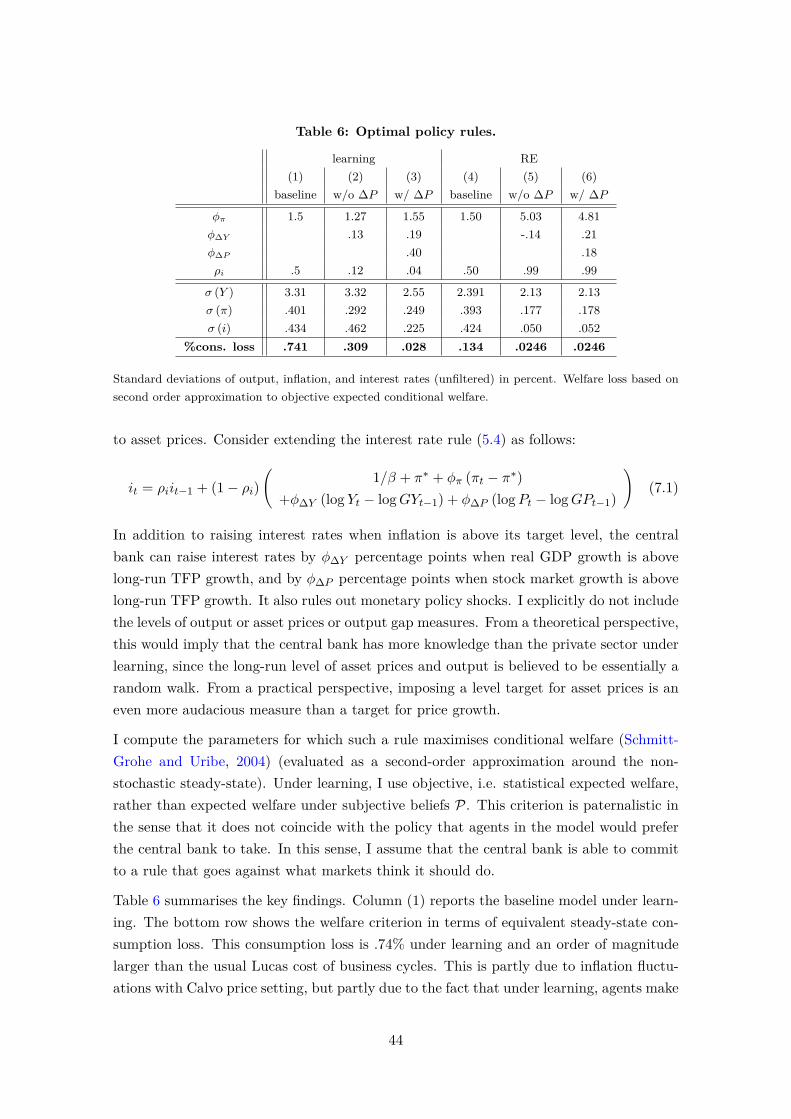
Table 6: Optimal policy rules.
learning RE(1) (2) (3) (4) (5) (6)
baseline w/o ∆P w/ ∆P baseline w/o ∆P w/ ∆P
φπ 1.5 1.27 1.55 1.50 5.03 4.81φ∆Y .13 .19 -.14 .21φ∆P .40 .18ρi .5 .12 .04 .50 .99 .99
σ (Y ) 3.31 3.32 2.55 2.391 2.13 2.13σ (π) .401 .292 .249 .393 .177 .178σ (i) .434 .462 .225 .424 .050 .052
%cons. loss .741 .309 .028 .134 .0246 .0246
Standard deviations of output, inflation, and interest rates (unfiltered) in percent. Welfare loss based onsecond order approximation to objective expected conditional welfare.
to asset prices. Consider extending the interest rate rule (5.4) as follows:
it = ρiit−1 + (1− ρi)(
1/β + π∗ + φπ (πt − π∗)+φ∆Y (log Yt − logGYt−1) + φ∆P (logPt − logGPt−1)
)(7.1)
In addition to raising interest rates when inflation is above its target level, the centralbank can raise interest rates by φ∆Y percentage points when real GDP growth is abovelong-run TFP growth, and by φ∆P percentage points when stock market growth is abovelong-run TFP growth. It also rules out monetary policy shocks. I explicitly do not includethe levels of output or asset prices or output gap measures. From a theoretical perspective,this would imply that the central bank has more knowledge than the private sector underlearning, since the long-run level of asset prices and output is believed to be essentially arandom walk. From a practical perspective, imposing a level target for asset prices is aneven more audacious measure than a target for price growth.
I compute the parameters for which such a rule maximises conditional welfare (Schmitt-Grohe and Uribe, 2004) (evaluated as a second-order approximation around the non-stochastic steady-state). Under learning, I use objective, i.e. statistical expected welfare,rather than expected welfare under subjective beliefs P. This criterion is paternalistic inthe sense that it does not coincide with the policy that agents in the model would preferthe central bank to take. In this sense, I assume that the central bank is able to committo a rule that goes against what markets think it should do.
Table 6 summarises the key findings. Column (1) reports the baseline model under learn-ing. The bottom row shows the welfare criterion in terms of equivalent steady-state con-sumption loss. This consumption loss is .74% under learning and an order of magnitudelarger than the usual Lucas cost of business cycles. This is partly due to inflation fluctu-ations with Calvo price setting, but partly due to the fact that under learning, agents make
44

choices that are optimal under subjective beliefs but highly suboptimal when evaluatedunder the objective probability measure. Column (2) calculates the welfare-maximisingrule that does not include a reaction to asset prices (φ∆P = 0). This makes it possible tocut the welfare loss by more than half, to .31%; however, output and stock price volatilityremain high. A reaction to stock price growth, however, is able to deliver substantialadditional stabilisation. The coefficient φ∆P is large and positive: A quarter-over-quarterincrease in stock prices by 1% is met with an interest rate rise of almost 0.4%. This doesnot mean, however, that the central bank interest rate is itself very volatile. In fact, thestandard deviations of output, stock prices, and interest rates are considerably reduced.By raising interest rates in a stock price boom, the central bank lowers aggregate demandand raises the cost of borrowing for firms, which both act to reduce corporate profits. Thiscurbs investor optimism in the stock market, thus dampening the feedback loop betweenbeliefs, prices, and profits.
This result is specific to the learning equilibrium and is not obtained under rational ex-pectations, as shown in Columns (4) to (6). When learning is shut down, the welfare costof business cycles for the baseline parameterisation is already much lower to start with.Optimising over the reaction to inflation and output growth alone, the central bank canalready effectively stabilise the economy and reduce the welfare loss considerably. Column(6) shows that when φ∆P is unconstrained, then the optimal rule is calculated to includea positive reaction to asset price growth as well. However, the added benefit of doing so isnegligible, with the welfare cost virtually unchanged. Hence, under rational expectations,a monetary policy reaction to asset prices carries no benefits.
8 Conclusion
This paper has analysed the implications of a learning-based asset pricing theory in abusiness cycle model with financial frictions. When firms borrow against the market valueof their assets, learning in the stock market interacts with credit frictions to form a two-sided feedback loop between beliefs, stock prices and firm profits that amplifies the assetprice dynamics.
I have embedded the mechanism in a dynamic stochastic general equilibrium model withnominal rigidities. Unlike most of the literature on adaptive learning, beliefs retained ahigh degree of rationality and internal consistency. In the baseline calibration of the model,introducing learning was shown to considerably improve the model’s asset price properties,notably volatility and return predictability, while still matching standard business cyclestatistics. At the same time, it leads to a large amount of propagation and amplificationof both supply and demand shocks, endogenising up to one third of the volatility of thebusiness cycle.
A natural criticism of a theory based on beliefs other than rational expectations is that ithas many degrees of freedom to adjust for almost any fact of choice. However, the present
45

model only introduces a single degree of freedom, the learning gain g, which is calibratedto the relative volatility of stock prices over dividends. Moreover, the predictable biases inforecasts made by agents in the model correspond surprisingly well to the patterns foundin actual data from surveys.
The model was also used to study normative implications of learning. In particular,I have revisited the question of whether monetary policy should react systematically toasset prices. I found that a strong reaction to stock price growth is desirable from a welfareperspective when investors in financial markets are learning. In contrast, under rationalexpectations, such a reaction does not improve welfare, in line with previous findingsin the literature. This illustrates the importance of asset pricing for macroeconomics.Assumptions about the source of volatility in financial markets has profound consequencesfor our policy recommendations.
While this paper mainly argues that improving asset price dynamics in a macroeconomicmodel can lead to novel insights about business cycles, future work should explore the otherdirection: Can a model of learning in a production economy teach us something new aboutasset pricing? I suspect that the endogenous feedback between beliefs and real activitymight provide for insights into the predictability of dividend growth vs the predictabilityof returns. It could also be worthwhile to explore extensions to the learning mechanism(such as a different perceived law of motion for prices, or learning about returns) thatmight further improve the asset price characteristics, a greater persistence of the P/Dratio and possibly even account for the equity premium.
But the analysis of this model need not be restricted to the role of stock prices affectinginvestment. Prices of other assets, for example housing, are also known to exhibit patternsthat are difficult to reconcile with the simple asset pricing models used commonly in themacro literature. At the same time, they clearly play a crucial role in affecting businesscycle fluctuations through credit constraints. A learning-based approach is likely to befruitful in this context.
46
References
Adam, K., Beutel, J. andMarcet, A. (2014). Stock Price Booms and Expected CapitalGains. Working paper.
—, Kuang, P. and Marcet, A. (2012). House price booms and the current account.NBER Macroeconomics Annual, 26 (1), 77–122.
— and Marcet, A. (2011). Internal rationality, imperfect market knowledge and assetprices. Journal of Economic Theory, 146 (3), 1224–1252.
—, — and Nicolini, J. P. (2013). Stock Market Volatility and Learning. Working Paper336, Barcelona Graduate School of Economics.
Altman, E. I. (2014). The role of distressed debt markets, hedge funds and recent trendsin bankruptcy on the outcomes of chapter 11 reorganizations. American BankruptcyInstitute Law Review, 22 (1), 75–267.
Bansal, R. and Yaron, A. (2004). Risks for the long run: A potential resolution of assetpricing puzzles. Journal of Finance, 59 (4), 1481–1509.
Barberis, N., Greenwood, R. M., Jin, L. J. and Shleifer, A. (forthcoming). X-capm: An extrapolative capital asset pricing model. Journal of Financial Economics,(19189).
Barro, R. (1990). The stock market and investment. Review of Financial Studies, 3 (1),115–131.
Beaudry, P. and Portier, F. (2006). Stock prices, news, and economic fluctuations.American Economic Review, 96 (4), 1293–1307.
Bernanke, B. S. and Gertler, M. (2001). Should central banks respond to movementsin asset prices? American Economic Review, 91 (2), pp. 253–257.
—, — andGilchrist, S. (1999). The financial accelerator in a quantitative business cycleframework. In J. B. Taylor and M.Woodford (eds.), Handbook of Macroeconomics, vol. 1,21, Elsevier, pp. 1341–1393.
Blanchard, O., Rhee, C. and Summers, L. (1993). The stock market, profit, andinvestment. Quarterly Journal of Economics, 108 (1), 115–136.
Boldrin, M., Christiano, L. J. and Fisher, J. D. M. (2001). Habit persistence, assetreturns, and the business cycle. American Economic Review, 91 (1), pp. 149–166.
Campbell, J. Y. and Cochrane, J. H. (1999). By force of habit: A consumption-basedexplanation of aggregate stock market behavior. Journal of Political Economy, 107 (2),pp. 205–251.
47
Caputo, R., Medina, J. P. and Soto, C. (2010). The Financial Accelerator UnderLearning and The Role of Monetary Policy. Working Papers of the Central Bank ofChile 590, Central Bank of Chile.
Cecchetti, S. G., Genberg, H. and Wadhwani, S. (2002). Asset Prices in a FlexibleInflation Targeting Framework. Working Paper 8970, NBER.
Cochrane, J. (1992). Explaining the variance of price-dividend ratios. Review of Finan-cial Studies, 5 (2), 243–280.
Coibion, O. andGorodnichenko, Y. (2010). Information Rigidity and the ExpectationsFormation Process: A Simple Framework and New Facts. Working Paper 16537, NBER.
Cordoba, J.-C. and Ripoll, M. (2004). International Economic Review, 45 (4), pp.1011–1046.
Covas, F. and Den Haan, W. J. (2012). The role of debt and equity finance over thebusiness cycle. Economic Journal, 122 (565), 1262–1286.
Croce, M. M. (2014). Long-run productivity risk: A new hope for production-basedasset pricing? Journal of Monetary Economics, 66 (0), 13–31.
Epstein, L. G., Farhi, E. and Strzalecki, T. (2013). How Much Would You Pay toResolve Long-Run Risk? Working Paper 19541, NBER.
Eusepi, S. and Preston, B. (2011). Expectations, learning, and business cycle fluctu-ations. American Economic Review, 101 (6), 2844–2872.
Faia, E. and Monacelli, T. (2007). Optimal interest rate rules, asset prices, and creditfrictions. Journal of Economic Dynamics and Control, 31 (10), 3228–3254.
Fama, E. F. and French, K. R. (1988). Dividend yields and expected stock returns.Journal of Financial Economics, 22 (1), 3–25.
Filardo, A. J. (2001). Should Monetary Policy Respond to Asset Price Bubbles? SomeExperimental Results. Research Working Paper RWP 01-04, Federal Reserve Bank ofKansas City.
Flynn, E. and Crewson, P. (2009). Chapter 11 filing trends in history and today.American Bankruptcy Institute Journal, 14, 65.
Gali, J. (2014). Monetary policy and rational asset price bubbles. American EconomicReview, 104 (3), 721–752.
Gelain, P., Lansing, K. J. andMendicino, C. (2013). House prices, credit growth, andexcess volatility: Implications for monetary and macroprudential policy. InternationalJournal of Central Banking, 9 (2), 219–276.
48
Gourio, F. (2012). Disaster risk and business cycles. American Economic Review,102 (6), 2734–2766.
Greenwood, R. and Shleifer, A. (2014). Expectations of returns and expected returns.Review of Financial Studies, 27 (3), 714–746.
Iacoviello, M. (2005). House prices, borrowing constraints, and monetary policy in thebusiness cycle. American Economic Review, 95 (3), 739–764.
Kimball, M. S., Fernald, J. G. and Basu, S. (2006). Are technology improvementscontractionary? American Economic Review, 96 (5), 1418–1448.
Lawton, A. (2012). Chapter 11 triage: Diagnosing a debtor’s prospects for success.Arizona Law Review, 54 (4), 985–1028.
Lettau, M. and Uhlig, H. (2000). Can habit formation be reconciled with business cyclefacts? Review of Economic Dynamics, 3 (1), 79–99.
Liu, Z., Wang, P. and Zha, T. (2013). Land-price dynamics and macroeconomic fluc-tuations. Econometrica, 81 (3), 1147–1184.
Maussner, A. (2010). The Analytics of New Keynesian Phillips Curves. Discussion PaperSeries 313, Universitaet Augsburg, Institute for Economics.
Mehra, R. and Prescott, E. C. (1985). The equity premium: A puzzle. Journal ofMonetary Economics, 15 (2), 145–161.
Milani, F. (2011). Expectation shocks and learning as drivers of the business cycle.Economic Journal, 121 (552), 379–401.
Sargent, T. J. (2008). Rational expectations. In D. R. Henderson (ed.), The ConciseEncyclopedia of Economics, 2nd edn., Library of Economics and Liberty.
Schmitt-Grohe, S. and Uribe, M. (2004). Solving dynamic general equilibrium mod-els using a second-order approximation to the policy function. Journal of EconomicDynamics and Control, 28 (4), 755–775.
Shiller, R. (1981). Do stock prices move too much to be justified by subsequent changesin dividends? American Economic Review, 71 (3), 421–436.
Tallarini Jr., T. D. (2000). Risk-sensitive real business cycles. Journal of MonetaryEconomics, 45 (3), 507–532.
Warren, E. and Westbrook, J. L. (2009). The success of chapter 11: A challenge tothe critics. Michigan Law Review, 107 (4), 604–641.
Xu, Z.,Wang, P. andMiao, J. (2013). A Bayesian DSGE Model of Stock Market Bubblesand Business Cycles. 2013 Meeting Papers 167, Society for Economic Dynamics.
49

A Further details on the full model
Retailers
Retailers transform a homogeneous intermediate good into differentiated final consumptiongoods using a one-for-one technology. The intermediate good trades in a competitivemarket at the real price qt (expressed in units of the composite final good). Each retailerenjoys market power in her output market though, and sets a nominal price pit for herproduction. A standard price adjustment friction à la Calvo means that a retailer cannotadjust her price with probability αp, which is independent across retailers and across time.Hence, the retailer solves the following optimisation:
maxPit
∞∑s=0
(s∏
τ=1κΛt+τ
)((1 + τ)Pit − qt+sPt+s)Yit+s
s.t. Yit =(PitPt
)−σYt
where Qt,t+s is the nominal discount factor of households between time t and t+ s and Ytis aggregate demand for the composite final good. Since all retailers that can re-optimiseat t are identical, they all choose the same price Pit = P ∗t . Since I want to evaluatewelfare in the model, I cannot log-linearise the first-order conditions of this problem.Their derivation is nevertheless standard (for example Maussner, 2010) and I only reportthe final equations here:
P ∗tPt
= 11 + τ
σ
σ − 1Γ1tΓ2t
(A.1)
Γ1t = qt + κEPt Λt+1Yt+1
Ytπσt+1 (A.2)
Γ2t = 1 + κEPt Λt+1Yt+1
Ytπσ−1t+1 (A.3)
I assume that the government sets subsidies such that τ = 1/(σ − 1) so that the steady-state markup over marginal cost is zero. Inflation and the reset price are linked throughthe price aggregation equation which can be written as:
1 = (1− κ)(P ∗tPt
)1−σ+ κπσ−1
t (A.4)
and the Tak-Yun distortion term is
∆t = (1− κ)(Γ1t
Γ2t
)−σ+ κπσt ∆t−1. (A.5)
This term ∆t ≥ 1 is the wedge due to price distortions between the amount of intermediategoods produced and the amount of the final good consumed.
50
Labour agencies
Similarly to retailers, labour agencies transform the homogeneous household labour inputinto differentiated labour goods at the nominal price wtPt and sell them to intermediatefirms at the price Wht. Labour agency h solves the following optimisation:
maxWht
EPt∞∑s=0
(s∏
τ=1κwΛt+τ
)((1 + τw)Wht − wt+sPt+s)Lht+s
s.t. Lht =(Wht
Wt
)−σwLt
Since all labour agencies that can re-optimise at t are identical, they all choose the sameprice Wht = W ∗t . The first-order conditions are analogous to those for retailers. Again, Iassume that the government sets taxes such that τ = 1/(σw − 1) so that the steady-statemarkup over marginal cost is zero. Wage inflation πwt and the Tak-Yun distortion ∆wt aredefined in the same way as for retailers. Finally, the real wage that intermediate producerseffectively pay is
wt = Wt
Pt= wt−1
πwtπt. (A.6)
Capital good producers
Capital good producers operate competitively in input and output markets, producingnew capital goods using old final consumption goods. For the latter, they have a CESaggregator just like households. Their maximisation programme is entirely intratemporal:
maxIt
QtIt −(It + ψ
2
(ItIt−1
− 1)2)
In particular, they take past investment levels It−1 as given when choosing current invest-ment output. Their first-order conditions defines the price for capital goods:
Qt = 1 + ψ
(ItIt−1
− 1)
(A.7)
51

Market clearing
The market clearing conditions are summarised below. Supply stands on the left-handside, demand on the right-hand side.
Yt =ˆ 1
0Yjtdj =
ˆ 1
0Yitdi (A.8)
Yt = Yt∆t
= Ct + It +−ψ2
(ItIt−1
− 1)2
+ Cet (A.9)
Lt =ˆ 1
0Lhtdh (A.10)
Lt = Lt∆wt
=ˆ 1
0Ljtdj (A.11)
Kt =ˆ 1
0Kjtdj = (1− δ)Kt−1 + It (A.12)
1 = Sjt, j ∈ [0, 1] (A.13)
0 = Bgt (A.14)
B Properties of the rational expectations equilibrium
The rational expectations equilibrium considered here has the following properties thatneed to be verified. All statements are local in the sense that for each of them, there existsa neighbourhood of the non-stochastic steady-state in which the statement holds.
1. All firms choose the same capital-labour ratio Kjt/Ljt .
2. The expected return on capital is higher than the internal return on debt: EtRkt+1 >
Rt.
3. At any time t, the stock market valuation Pjt of a firm j is proportional to its networth after entry and exit Njt with a slope that is strictly greater than one.
4. Borrowers never default on the equilibrium path and borrow at the risk-free rate,and the lender only accepts debt payments up to a certain limit.
5. If the firm defaults and the lender seizes the firm, she always prefers restructuringto liquidation.
6. The firm always exhausts the borrowing limit.
7. All firms can be aggregated. Aggregate debt, capital and net worth are sufficient todescribe the intermediate goods sector.
I take the following steps to prove existence of this equilibrium. After setting up thefirm value functions, Property 1 just follows from constant returns to scale. I then take
52

Properties 2 and 3 as given and prove 4 to 6. I verify that 3 holds. The aggregationproperty 7 is then easily verified. I conclude by establishing the parameter restrictions forwhich 2 holds.
Value functions
An operating firm j enters period t with a predetermined stock of capital and debt. It isconvenient to decompose its value function into two stages. The first stage is given by:
Υ1 (K,B) = maxN,L,D
γN + (1− γ) (D + Υ2 (N −D))
s.t. N = qY − wL+ (1− δ)QK −RB
Y = Kα (AL)1−α
D = ζ (N −QK +B)
(I suppress the time and firm indices for the sake of notation.) After production, the firmexits with probability γ and pays out all net worth as dividends. The second stage ofthe value function consists in choosing debt and capital levels as well as a strategy in thedefault game:
Υ2(N)
= maxK′,B′,strategy in default game
βE[Υ1(K ′, B′
), no default
]+ βE
[Υ1(K ′, B∗
), debt renegotiated
]+ βE [0, lender seizes firm]
s.t. K ′ = N +B′
A firm which only enters in the current period starts directly starts with an exogenous networth endowment and the value function Υ2.
Characterising the first stage
The first order conditions for the first stage with respect to L equalises the wage with themarginal revenue: w = q (1− α) (K/L)αA1−α. Since there is no firm heterogeneity apartfrom capital K and debt B, this already implies Property 1 that all firms choose the samecapital-labour ratio. Hence the internal rate of return on capital is also common acrossfirms:
Rk = αq
((1− α) qA
w
) 1−αα
+ (1− δ)Q (B.1)
53

Now taking Property 3 as given (and verifying it later on), Υ2 is a linear function withslope strictly greater than one. Then the following holds for the first-stage value functionΥ1:
Υ1 (K,B) = N + (1− γ) (D −N + Υ2 (N −D))
= N + (1− γ)(Υ ′2 − 1
)((1− ζ)N + ζ (QK −B))
> N
= RkK −RB (B.2)
This property will be used repeatedly in the next step of the proof.
Characterising the second stage
The second stage involves solving for the subgame-perfect equilibrium of the default gamebetween borrower and lender. Pairings are anonymous, so repeated interactions are ruledout. Also, only the size B and the interest rate R of the loan can be contracted (I omitprimes for ease of notation and separate R from the risk-free rate R). The game is playedsequentially:
1. The firm (F) proposes a borrowing contract(B, R
).
2. The lender (L) can accept or reject the contract.
• A rejection corresponds to setting the contract(B, R
)= (0, 0).
Payoff for L: 0. Payoff for F: βE[Υ1(N , 0
)].
3. F acquires capital and can then choose to default or not.
• If F does not default, it has to repay in the next period.Payoff for L: EQt,t+1RB −B. Payoff for F: βE
[Υ1(K, RRB
)].
4. If F defaults, the debt needs to be renegotiated. F makes an offer for a new debtlevel B∗.26
5. L can accept or reject the offer.
• If L accepts, the new debt level replaces the old one.Payoff for L: EΛRB∗ −B. Payoff for F: βE
[Υ1(K, RRB
∗)].
6. If L rejects, then she seizes the firm. A fraction 1− ξ of the firm’s capital is lost inthe process. Nature decides randomly whether the firm can be “restructured”.
26That the interest rate on the repayment is fixed is without loss of generality.
54

• If the firm cannot be restructured, or it can but the lender chooses not to doso, then the lender has to liquidate the firm.Payoff for L: EΛξQK −B. Payoff for F: 0.
• If the firm can be restructured and the lender chooses to do so, she retains adebt claim of present value ξB and sells the residual equity claim in the firmto another investor.Payoff for L: ξB + βE [Υ1 (ξK, ξB)]−B. Payoff for F: 0.
Backward induction leads to the (unique) subgame-perfect equilibrium of this game. Startwith the possibility of restructuring. The lender L prefers this to liquidation if
ξB + βE [Υ1 (ξK, ξB)] ≥ EΛξQK. (B.3)
This holds true at the steady state because Rk > R (Property 2), Q = 1, β = Λ and
ξB + βE [Υ1 (ξK, ξB)] > ξB + βE[RkξK −RξB
]= βE
[RkξK
]> ξK (B.4)
Since the inequality is strict, the statement holds in a neighbourhood around the steady-state as well. This establishes Property 5.
Next, the lender L will accept an offer B∗ if it gives her a better expected payoff (assumingthat lenders can diversify among borrowers so that their discount factor is invariant to theoutcome of the game). The probability of restructuring is given by x. The condition foraccepting B∗ is therefore that
EΛRB∗ ≥ x(ξB + βE [Υ1 (ξK, ξB)]
)+ (1− x)EΛξQK. (B.5)
Now turn to the firm F. Among the set of offers B∗ that are accepted by L, the firm willprefer the lowest one, i.e. that which satisfies (B.5) with equality. This follows from Υ1
being a decreasing function of debt. This lowest offer will be made if it leads to a higherpayoff than expropriation: βE
[Υ1(K, RRB
∗)]≥ 0. Otherwise, the firm offers zero and the
lender seizes the firm.
Going one more step backwards, the firm has to decide whether to declare default or not.It is preferable to do so if the B∗ that the lender will just accept is strictly smaller thanB or if expropriation is better than repaying, βE
[Υ1(K, RRB
)]≥ 0.
What is then the set of contracts which the lender L accepts in the first place? From theperspective of L, there are two types of contracts: those that will not be defaulted on andthose that will. If the firm does not default (B∗ ≥ B), the lender will accept the contractsimply if it pays at least the risk-free rate, R ≥ R. If the firm does default (B∗ < B), then
55

the lender accepts if the expected discounted recovery value exceeds the size of the loan,i.e. EΛRB∗ ≥ B.
Finally, let’s consider the contract offer by the firm. Firm F can offer a contract on whichit will not default. In this case, it is optimal to offer just the risk-free rate R = R. Alsonote that the payoff from this strategy is strictly positive since
βE [Υ1 (K,B)] > βE[RkK −RB
]= βE
[RkN +
(Rk −R
)B]
> 0. (B.6)
The payoff is also increasing in the size of the loan B. So conditional on not defaulting,it is optimal for F to take out the maximum loan size B = B∗, and this is preferable todefault with expropriation. However, it might also be possible for F to offer a contractthat only leads to a default with debt renegotiation. The optimal contract of this type isthe solution to the following problem:
maxR,B,B∗
βE[Υ1
(N +B,
R
RB∗)]
s.t. EΛRB∗ ≥ B
EΛRB∗ = x(ξB + βE
[Υ1(ξ(N +B
), ξB
)])+ (1− x)EΛQξ
(N +B
)The first thing to note is that only the product RB∗ appears, so the choice of the interestrate R is redundant. Further, B = B∗ and R = R solve this problem, and this amountsto the same as not declaring default. This choice solves the maximisation problem aboveif the following condition is satisfied at the steady state:
ξ
R
(1− x+ xR+ xΥ ′1
[Rk
R− 1
])< 1 (B.7)
For the degree of stock price dependence x sufficiently small, this condition is satisfied.This establishes Properties 4 and 6.
Linearity of firm value
Since firms do not default and exhaust the borrowing limit B∗, the second-stage firm valuecan be written as follows:
Υ2(N)
= βE[Υ1(N +B,B
)](B.8)
where B = x(ξB + βE
[Υ1(ξ(N +B
), ξB
)])+ (1− x)Qtξ
(N +B
)(B.9)
56

We already know that if Υ2 is a linear function, then Υ1 is also linear. The converse alsoholds: The constraint above together with linearity of Υ1 imply that B is linear in N , andthus Υ2 is linear, too.
To establish Property 3, it remains to show that the slope of Υ2 is greater than one. Thisis easy to see in steady state:
Υ ′2 = βΥ1 (K,B)
N
= βγ(RkK −RB
)+ (1− γ)Υ2
(RkK −RB
)N
= β(γ + (1− γ)Υ ′2
) (Rk
K
N−RB
N
)
=(γ + (1− γ)Υ ′2
) Rk +(Rk −R
)BN
R︸ ︷︷ ︸=:c0>1
= γc01− (1− γ) c0
> 1 (B.10)
Finally, the aggregated law of motion for capital and net worth need to be established(Property 7). Denoting again by Γt ⊂ [0, 1] the indices of firms that exit and are replacedin period t, we have:
Kt =ˆ 1
0Kjtdj =
ˆj /∈Γt
(Njt − ζEjt +Bjt) dj +ˆj∈Γt
(ω (Nt − ζEt) +Bjt) dj
= (1− γ + γω) (Nt − ζEt) +Bt (B.11)
Nt =ˆ 1
0Njtdj = RktKt−1 −Rt−1Bt−1 (B.12)
Bt =ˆ 1
0Bjtdj = xξ (Bt + Pt) + (1− x) ξEtΛt+1Qt+1Kt (B.13)
So far then, all model properties are established except for Rk > R.
Return on capital
It can now be shown under which conditions the internal rate of return is indeed greaterthan the return on debt. From the steady-state versions of equations (B.11) and (B.12),it follows that
Rk = R+ (G−R (1− γ + γω)) NK
+Rc (1− γ + γω) EK. (B.14)
57

Sufficient conditions for Rk > R are therefore that N/K and E/K are strictly positiveand that the following holds:
γ >R−G
G (1− ω) (B.15)
C Approximation method for the learning equilibrium
The second order perturbation method for the learning equilibrium follows Schmitt-Groheand Uribe (2004), but has to be adapted to allow for relaxation of the rational expectationsassumption. A rational expectations equilibrium can generally be described as a solution(yt)t∈N to
Et [f (yt+1, yt, xt, ut)] = 0. (C.1)
where Et is the expectations operator with respect to the probability measure and filtrationinduced by exogenous stochastic disturbances ut. These disturbances are of dimensionalitynu, independent and identically distributed, of zero mean and variance σ2Σu. The solutionyt is of dimensionality n, as is the image of f . xt denotes a vector of predetermined statevariables of dimensionality nx < n: xi,t = yι(i),t−1 for an injective ι : {1..n} → {1..nx},or simply xt = Cyt−1 for an appropriate matrix C. One is interested in finding a policyfunction that generates solutions of the form
yt = g (xt, ut, σ) . (C.2)
Perturbation methods for approximating the policy function to higher orders are straight-forward. They compute Taylor expansions of g, typically around a non-stochastic steadystate of the model , i.e. a constant solution y for σ = 0 such that f (y, y, x, 0) = 0 andhence g (y, 0, 0) = y.
In a learning equilibrium, (C.1) does not fully characterise the equilibrium because theprobability measure used by agents to form expectations does not coincide with the actualprobability measure of the model. The stock price in the model of this paper is determinedby the usual market-clearing condition, but agents think it is determined by randomunforecastable shocks that are not necessarily related to the rest of the economy. A modeldescribed by (C.1) cannot contain a shock that is perceived as exogenous but at the sametime determined endogenously.
The model in this paper belongs to a class that can be written as follows:
EPt [f (yt+1, yt, xt, ut, zt)] = 0 (C.3)
EPt [φ (yt+1, yt, xt, ut, zt)] = 0 (C.4)
Here, the probability measure P denotes beliefs for which the disturbances zt (of dimen-sionality nz) are perceived as exogenous, independent and identically distributed withzero mean and variance σ2Σz. They are also perceived as independent of ut, although
58

this can be relaxed. These disturbances have the interpretation of forecast errors. Theiid assumption then amounts to imposing that agents holding the belief P think theirforecasts cannot be improved upon. As before, f is of dimensionality n. The system (C.3)is assumed to have a unique solution for each initial condition xt and path of disturbancesut and zt which can be described by a subjective policy function:
yt = h (xt, ut, zt, σ) (C.5)
Contrary to agents’ beliefs, zt is not an exogenous disturbance, but determined endogen-ously by the second set of equilibrium conditions (C.4). The function φ is of dimensionnz. This set of conditions is not known to agents. The actual probability measure P0,induced by (C.3)-(C.4) and the disturbances ut, is thus different from P. Under P0, zt isa function of the state and the fundamental disturbances:
zt = r (xt, ut, σ) (C.6)
This leads to the objective policy function:
g (xt, ut, σ) = h (xt, ut, r (xt, ut, σ) , σ) (C.7)
All functional forms are assumed to be such that the functions h and r are uniquelydetermined.
In the case of the model of this paper, lagged belief updating requires two pseudo-disturbances, nz = 2. Agents cannot update their beliefs about future stock prices atthe same time as they observe current prices, yet by observing the price they can infer thecurrent forecast error. This implies the following subjective belief equations that are partof (C.3):
logPt = logPt−1 + µt−1 −σ2η + σ2
ν
2 + z1t (C.8)
µt = µt−1 −σ2ν
2 + gz2t (C.9)
The conditions (C.4) that pin down the values for the forecast errors zt in equilibrium arethen described as follows:
Pt − βEPt [Dt+1 + Pt+1] = 0 (C.10)
z2t − z1t−1 = 0 (C.11)
Going back to the general case, the goal is to derive an accurate second-order approxim-
59

ation of the objective policy function g around the non-stochastic steady state:
g (xt, ut, σ) ≈ g (x, 0, 0)
+ gx (xt − x) + guut
+ 12gxx [(xt − x)⊗ (xt − x)] + 1
2gxu [(xt − x)⊗ ut] + 12guu [ut ⊗ ut]
+ 12gσσσ
2 (C.12)
The first step in deriving the approximation consists in calculating this approximation forthe subjective policy function h. This can be done using standard methods as describedin Schmitt-Grohe and Uribe (2004) and implemented e.g. in Dynare. The second stepconsists in finding the derivatives of the function r in (C.6). Substituting it into theequilibrium conditions (C.4) gives:
0 = Φ (x, u, σ) = EPt[φ(y′, y, x, u, z
)]= EPt
φ h (Ch (x, u, z, σ) , u′, z′, σ) ,
h (x, u, z, σ) , x, u, z
= EPt
φ h (Ch (x, u, r (x, u, σ) , σ) , u′, z′, σ) ,h (x, u, r (x, u, σ) , σ) , x, u, r (x, u, σ)
(C.13)
Here, I drop time subscripts and denote by a prime variables at t+ 1. Note that the termz′ must not be substituted out when the expectation is taken under P. Doing so wouldimply that agents know the true relationship between zt+1 and the model variables insteadof taking it as an exogenous disturbance. Total differentiation at the non-stochastic steadystate leads to the following first-order derivatives:
0 = dΦdx
(x, 0, 0) =(φy′hxC + φy
)(hx + hzrx) + φx + φzrx (C.14)
0 = dΦdu
(x, 0, 0) =(φy′hxC + φy
)(hu + hzru) + φu + φzru (C.15)
0 = dΦdσ
(x, 0, 0) =(φy′hxC + φy
)(hσ + hzrσ) + φzrσ (C.16)
Since the existence of a unique solution for r is assumed, the first derivatives can be solvedfor. I also assume that the equilibrium conditions imply that z = 0 at the steady-state.This means that in the absence of shocks, agents make no forecast errors under learning.
Define the matrix A =(φy′hxC + φy
)hz + φz. Then the first-order derivatives of r are
60

given by:
rx = −A−1 ((φy′hxC + φy)hx + φx
)(C.17)
ru = −A−1 ((φy′hxC + φy)hu + φu
)(C.18)
rσ = 0 (C.19)
Up to first order, the existence and uniqueness of the function r is equivalent to invertibilityof the matrix A. The first-order derivatives of the actual policy function g can be obtainedby applying the chain rule. The certainty-equivalence property holds for the subjectivepolicy function h, hence hσ = 0. This implies that rσ = 0 and gσ = 0 as well, so certaintyequivalence also holds under learning.
The second-order calculations are similar, if more tedious. The second-order derivative ofΦ with respect to x is:
0 = d2Φdx2 (x, 0, 0) =
(φy′gxC + φy
)(hxx + 2hxz [Inx ⊗ rx] + hzz [rx ⊗ rx])
+ φy′hxx [Cgx ⊗ Cgx] +Bxx +Arxx (C.20)
This equation isn2x-dimensional and linear in rxx, and thus can be solved easily. As in
first order, only invertibility of the matrix A is required for a unique local solution underlearning. I have collected all cross-derivatives of φ inside the matrix Bxx (of size nz ×n2
x),which contains only first-order derivatives of the policy functions:
Bxx = φy′y′ [hxCgx ⊗ hxCgx] + φyy [gx ⊗ gx] + φxx + φzz [rx ⊗ rx]
+ 2φy′y [hxCgx ⊗ gx] + 2φy′x [hxCgx ⊗ Inx ] + 2φy′z [hxCgx ⊗ rx]
+ 2φyx [gx ⊗ Inx ] + 2φyz [gx ⊗ rx] + 2φxz [Inx ⊗ rx] (C.21)
The formulae to solve for rxu and ruu are analogous. It remains to look at the derivativesinvolving σ. This simplifies considerably because the first derivatives of the policy func-tions g and h with respect to σ are zero. The cross-derivative of Φ with respect to x andσ thus reads:
0 = d2Φdxdσ
(x, 0, 0) =(φy′gxC + φy
)(hxσ + hzrxσ) + φzrxσ (C.22)
But because hxσ = 0 as under rational expectations, rxσ = 0 holds as well. The sameapplies to ruσ = 0. Finally, the second derivative with respect to σ involves the varianceof the disturbances:
0 = d2Φdσ2 (x, 0, 0) = φy′y′ (hσσ + huuvec (Σu) + +hxxvec (Σz))
+ φy′y′(vec
(h′uΣuhu
)+ vec
(h′zΣzhz
))+
(φy′gxC + φy
)(hσσ) +Arσσ (C.23)
61

Again, this can be solved for rσσ when A is invertible. Note that the perceived varianceΣz appears in the calculation because it matters for expectations for the future (unlessφy′y′ = 0). This variance is not necessarily equal to the objective variance of z.
The second-order derivatives of the actual policy function g are calculated easily oncethose of r are known:
gxx = hxx + 2hxz [Inx ⊗ rx] + gzz [rx ⊗ rx] + gzrxx (C.24)
and analogously for gxu, guu and gσσ. The cross-derivatives guσ and gxσ are zero.
62