the role of learning for stock prices and business cycles
TRANSCRIPT

The Role of Learning for Stock Prices and BusinessCycles
Fabian Winkler∗
25 April 2016
Abstract
The effects of financial frictions in business cycle models depend heavilyon the underlying asset pricing theory. I examine the implications of learning-based asset pricing in a model in which firms face credit constraints that dependpartly on their market value. Agents are learning about stock prices, buthave conditionally model-consistent expectations otherwise. The model jointlymatches key asset price and business cycle statistics, while the combination offinancial frictions and learning produces powerful feedback between asset pricesand real activity, adding substantial amplification of business cycle shocks.Patterns of predictability in agents’ subjective forecast errors closely matchsurvey data.
JEL: D83, E32, E44, G12
Keywords: Learning, Expectations, Financial Frictions, Asset Pricing, Survey Data
Financial frictions are seen as a central mechanism by which asset prices interactwith macroeconomic dynamics. Yet our understanding of this interaction remainsincomplete, in part due to the inherent difficulty of modelling asset prices. Typicalbusiness cycle models still rely on an asset pricing theory based on rational expec-tations, time-separable preferences and moderate degrees of risk aversion. It is well
∗Board of Governors of the Federal Reserve System, 20th St and Constitution Ave NW, Wash-ington DC 20551, [email protected]. I thank Wouter den Haan for his guidance and support;Klaus Adam, Andrea Ajello, Johannes Boehm, Peter Karadi, Albert Marcet, Stephane Moyen,Rachel Ngai, Markus Riegler, and participants at the ECB-CFS-Bundesbank lunchtime seminar,Singapore Management University, Econometric Society Winter Meeting in Madrid, EEA AnnualMeeting in Toulouse, and Econometric Society World Congress in Montreal, for useful commentsand suggestions. The views herein are those of the author and do not represent the views of theBoard of Governors of the Federal Reserve System or the Federal Reserve System.
1

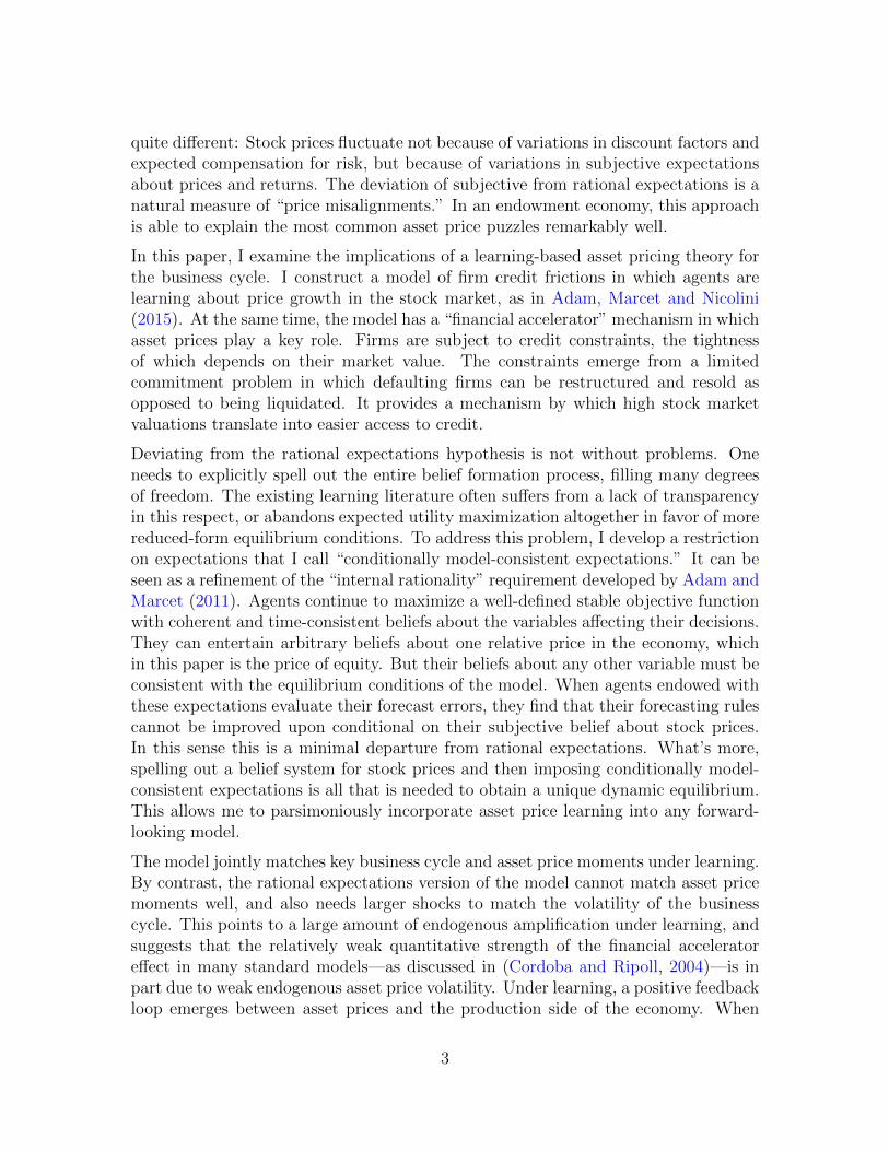
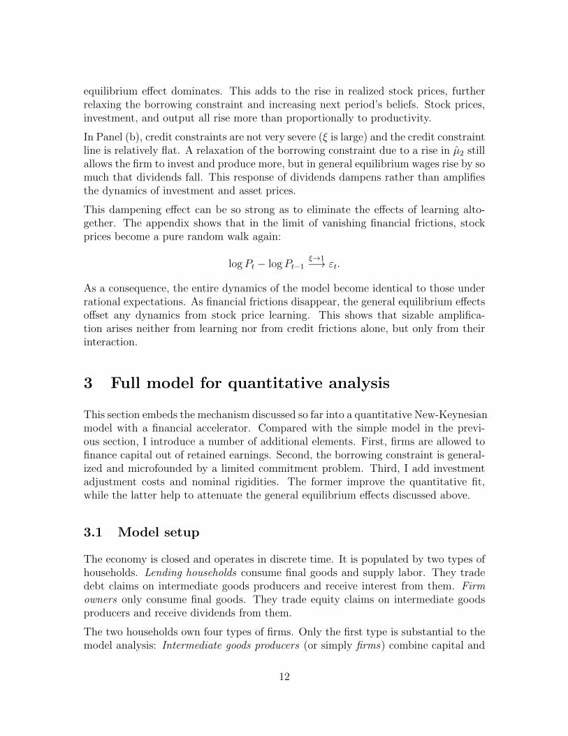
Figure 1: Return expectations and expected returns.
24
68
101-
year
ret
urn
fore
cast
3.5 4 4.5log P/D ratio
-60
-40
-20
020
401-
year
rea
lised
ret
urn
3.5 4 4.5log P/D ratio
Expected nominal returns (left) are the mean response in the Graham-Harvey survey, realized nom-inal returns (right) and P/D ratio are from the S&P 500. Data period 2000Q32012Q4. Correlationcoefficient for return forecasts ρ = .54, for realized returns ρ = −.44.
known that such a theory is inadequate for many empirical asset price regularities.At the same time, asset prices play a central role in macroeconomic dynamics in thepresence of financial frictions. Conclusions drawn from models with financial frictionsbut without a good asset pricing theory are therefore questionable.
There is not a shortage of theories that aim to explain asset price dynamics. Mostkeep the rational expectations assumption and engineer preferences that deliver highlyvolatile discount factors. There are however compelling arguments for relaxing therational expectations assumption instead. Measurements of expectations in surveysdo not support the rational expectations hypothesis. The hypothesis implies, forexample, that investors are fully aware of return predictability in the stock market,expecting lower returns when prices are high and vice versa. Instead, measuredexpectations imply they expect higher returns. This pattern has been documentedextensively by Greenwood and Shleifer (2014) and is illustrated in Figure 1. The leftpanel plots the mean 12-month return expectation of the S&P500, as measured in theGraham-Harvey survey of American CFOs, against the value of the P/D ratio in themonth preceding the survey. The correlation is strongly positive: Return expectationsare more optimistic when stock valuations are high. This contrasts sharply with theactual return predictability in the right panel of the figure, where the correlation isstrongly negative. Unless one rejects surveys as an unbiased measure of expectations,such a pattern cannot be reconciled with rational expectations.
Based on such observations, Adam, Marcet and Nicolini (2015) have developed anasset pricing theory based on learning. The interpretation of price dynamics there is
2
quite different: Stock prices fluctuate not because of variations in discount factors andexpected compensation for risk, but because of variations in subjective expectationsabout prices and returns. The deviation of subjective from rational expectations is anatural measure of “price misalignments.” In an endowment economy, this approachis able to explain the most common asset price puzzles remarkably well.
In this paper, I examine the implications of a learning-based asset pricing theory forthe business cycle. I construct a model of firm credit frictions in which agents arelearning about price growth in the stock market, as in Adam, Marcet and Nicolini(2015). At the same time, the model has a “financial accelerator” mechanism in whichasset prices play a key role. Firms are subject to credit constraints, the tightnessof which depends on their market value. The constraints emerge from a limitedcommitment problem in which defaulting firms can be restructured and resold asopposed to being liquidated. It provides a mechanism by which high stock marketvaluations translate into easier access to credit.
Deviating from the rational expectations hypothesis is not without problems. Oneneeds to explicitly spell out the entire belief formation process, filling many degreesof freedom. The existing learning literature often suffers from a lack of transparencyin this respect, or abandons expected utility maximization altogether in favor of morereduced-form equilibrium conditions. To address this problem, I develop a restrictionon expectations that I call “conditionally model-consistent expectations.” It can beseen as a refinement of the “internal rationality” requirement developed by Adam andMarcet (2011). Agents continue to maximize a well-defined stable objective functionwith coherent and time-consistent beliefs about the variables affecting their decisions.They can entertain arbitrary beliefs about one relative price in the economy, whichin this paper is the price of equity. But their beliefs about any other variable must beconsistent with the equilibrium conditions of the model. When agents endowed withthese expectations evaluate their forecast errors, they find that their forecasting rulescannot be improved upon conditional on their subjective belief about stock prices.In this sense this is a minimal departure from rational expectations. What’s more,spelling out a belief system for stock prices and then imposing conditionally model-consistent expectations is all that is needed to obtain a unique dynamic equilibrium.This allows me to parsimoniously incorporate asset price learning into any forward-looking model.
The model jointly matches key business cycle and asset price moments under learning.By contrast, the rational expectations version of the model cannot match asset pricemoments well, and also needs larger shocks to match the volatility of the businesscycle. This points to a large amount of endogenous amplification under learning, andsuggests that the relatively weak quantitative strength of the financial acceleratoreffect in many standard models—as discussed in (Cordoba and Ripoll, 2004)—is inpart due to weak endogenous asset price volatility. Under learning, a positive feedbackloop emerges between asset prices and the production side of the economy. When
3

beliefs of learning investors are more optimistic, their demand for stocks increases.This raises firm valuations and relaxes credit constraints, in turn allowing firms tomove closer to their profit optimum. Firms are able to pay higher dividends to theirshareholders, raising stock prices further and propagating investor optimism.
I then compare the subjective forecasts of agents in the model with actual forecastsin survey data. Even though agents only learn about stock prices in the model, theirexpectational errors spill over into forecasts of other variables. For example, whenagents are too optimistic about asset prices, they also become too optimistic aboutthe tightness of credit constraints and therefore over-predict future investment. Themodel-generated expectations replicate remarkably well the predictability of forecasterrors for several predictors and across a range of forecast variables.
In a series of sensitivity checks, I show that nominal rigidities greatly enhance theamplification effects of the feedback loop under learning. This is in part due totheir ability to generate comovement in macroeconomic aggregates following shiftsin borrowing constraints. The interest rate rule followed by the monetary authorityalso plays a role in the amplification mechanism. In particular, a positive response ofinterest rates to stock price growth is able to greatly reduce endogenous volatility byeffectively stabilizing asset price expectations.
The remainder of the paper is structured as follows. Section 1 briefly discusses therelated literature. Section 2 presents a simplified version of the model that permits ananalytic solution. It shows that credit frictions or asset price learning alone does notgenerate either amplification of shocks or interesting asset price dynamics, althoughtheir combination does. The full model is presented in Section 3. Section 4 containsthe quantitative results. Section 5 contains sensitivity checks, including the effects ofdifferent interest rate rules. Section 6 concludes.
1 Related literature
The early literature on financial frictions emphasized their role for amplyfing businesscycle shocks (Kiyotaki and Moore, 1997), but the quantitative importance of the“financial accelerator” mechanism is often found to be small (Quadrini, 2011). Themore recent literature on financial frictions instead emphasizes shocks to borrowingconstraints as independent drivers of the business cycle (e.g. Jermann and Quadrini,2012), or alternatively introduces direct shocks to asset prices. Xu, Wang and Miao(2013) develop a model in which borrowing limits depend on stock market valuationsthrough a credit friction similar to that in my model. They prove the existence ofrational liquidity bubbles and introduce a shock that governs the size of this bubble.Liu, Wang and Zha (2013) use a similar framework with land prices instead of stockprices. This paper takes a different approach by going back to the question of financialfrictions as an amplification mechanism. Learning endogenously generates volatility
4

in asset prices, and interacts with financial frictions to form a feedback loop thatamplifies standard business cycle shocks.
Besides learning, there exist of course other asset pricing theories to address assetpricing puzzles, including habit, long-run risk, and disaster risk. Each of them hasbeen shown to be compatible with standard business cycle moments in productioneconomies (Boldrin, Christiano and Fisher, 2001, for habit; Tallarini Jr., 2000, forlong-run risk; and Gourio, 2012, for disaster risk). But each of them also has itsproblems (e.g. Lettau and Uhlig 2000; Epstein, Farhi and Strzalecki 2013), and noneof them is able to explain the disconnect between statistically predicted returns andexpectations of returns in surveys. There is currently no consensus among economistswhich asset pricing theory is “best”, and the goal of this paper is not to set up a horserace between learning and alternative asset pricing theories. Rather, the goal is toexamine in detail the interaction of learning-based asset pricing and financial frictions.
There are a number of papers that study models of financial frictions in combinationwith learning (Caputo, Medina and Soto, 2010; Milani, 2011; Gelain, Lansing andMendicino, 2013). Their approach consists of two steps: first, derive the linearizedequilibrium conditions of the economy under rational expectations; second, replaceall terms involving expectations with parameterized forecast functions, and updatethe parameters every period. Such an approach certainly produces very rich dynam-ics, but is problematic on several grounds. First, such parameterized expectationequations often do not correspond anymore to intertemporal optimization problems.Second, the analysis of these models is often complex and lack transparency. Here, Idevelop a more transparent and parsimonious approach. Beliefs are restricted to beconditionally model-consistent and agents make optimal choices given a consistent setof beliefs. This preserves much of the intuition of a rational expectations model, andat the same time allows for “spillovers” of forecast errors on asset prices into otherforecasts. The approach also differs from that of Fuster, Hebert and Laibson (2012).There, agents learn only about exogenous variables, and endogenous outcomes cantherefore not feed back into beliefs. In this model, agents learn about endogenousprices, with a feedback loop between beliefs and real activity.
Finally, the paper relates to the research on survey data on expectations. It is wellknown that expectations measured in surveys fail to conform to the rational expecta-tions hypothesis because forecast errors are statistically predictable (e.g. Croushore,1997). Coibion and Gorodnichenko (2015) interpret forecast error predictability asevidence in favour of rational inattention models. The model in this paper producessimilar predictability statistics in a learning model.
5
2 Simplified model
In this section, I construct a simplified version of the model which illustrates theinteraction between credit frictions and learning about asset prices. For the sake ofbrevity, I omit a formal description of the model, which can be found in the appendix.The key insight is that neither learning nor financial frictions alone generate sizableamplification of business cycle shocks or asset price volatility in a production economy,while in combination they do.
2.1 Model setup
The economy consists of a representative household and a representative firm. Thereare two physical goods, labor and a consumption/investment good. The household isrisk-neutral with discount rate β. It inelastically supplies one unit of labor and alsoholds the debt and equity claims on the firm. Debt claims pay a gross real interestrate R. For the debt market to be in equilibrium, the interest rate has to equalR = 1/β. Equity claims trade at a price Pt and pay dividends Dt. For the stockmarket to be in equilibrium, the following Euler equation has to hold:
Pt = βEPt [Pt+1 +Dt+1] . (1)
Note that the expectation operator is evaluated under the probability measure P .Agents use this measure when forming their expectations to solve their optimizationproblems. Under learning, the distribution of outcomes expected under P does notnecessarily coincide with the distribution induced in equilibrium.
The representative firm operates a constant returns to scale technology in capitalKt−1 and labor Lt. Labor is hired at the competitive wage rate wt. The capital stockdepreciates at the rate δ and must be financed entirely with borrowed funds. Thefirm faces a leverage constraint by which its debt claims cannot exceed a fraction ξ ofits total market value (equity and debt). For simplicity, all earnings are assumed tobe paid out as dividends every period and the number of shares outstanding is fixedat unity. The firm maximizes expected dividends as follows:
EPt Dt+1 = maxKt,Lt+1
EPt[Kαt (At+1Lt+1)1−α − wt+1Lt+1 + (1− δ)Kt −RKt
](2)
s.t. 0 ≤ Kt ≤ξ
1− ξPt (3)
Note that the borrowing constraint (3) relates the level of the capital stock Kt (equalto the value of the firm’s outstanding debt) to the value of its equity. The microfoun-dation of this constraint is discussed in the next section. For the labor market to be
6

in equilibrium, the wage rate wt has to adjust such that the firm demands Lt = 1.Define the rationally expected return on capital as:
Rk (Kt, At) = α
(AtKt
)1−α
Et[ε1−αt+1
]+ 1− δ. (4)
Finally, the only exogenous shock in the model is a permanent innovation to produc-tivity, which evolves as:
logAt = logAt−1 + εt, εt ∼ iidN(−σ
2
2, σ2
). (5)
2.2 Rational expectations equilibrium
I first describe the equilibrium under rational expectations.1 Start with the case ξ = 1.In this limiting case, the borrowing constraint (3) can never bind. The firm invests upto the efficient level where the expected return on capital equals the interest rate. Asa result, capital is simply proportional to productivity: Kt/At = K∗ for some fixedvalue K∗.
Once we introduce financial frictions by setting ξ < 1, how much amplification dowe get? The answer is: none. For all values of ξ strictly below one, the borrowingconstraint is always binding, and the equilibrium is characterized by the followingtwo equations:
Pt = AtP = At
(Rk(K, 1
)−R
)K
R− 1(6)
Kt = AtK =ξ
1− ξPt (7)
The first equation pins down the stock market value of the firm, which depends onthe capital stock through expected dividends in the enumerator. These dividendsdepend on capital through the size of the firm and the rate of return on capital.The second equation determines the capital stock that can be reached by exhaustingthe borrowing constraint that depends on the stock market value. In the uniqueequilibrium, the capital stock is proportional to productivity, just as was the casewhen ξ = 1.
Financial frictions do not lead to any amplification or propagation of shocks in therational expectations equilibrium. They have a level effect on output, capital, etc.,but the dynamics of the model are identical for any value of ξ. Similarly, the behaviorof asset prices is entirely independent of ξ. The stock price evolves simply as:
logPt = logPt−1 + εt. (8)
1In a rational expectations equilibrium, the distribution of outcomes under P coincides with theequilibrium distribution of outcomes. In that case, one can write EP [·] = E [·].
7

Intuitively, with financial frictions, a shock to productivity raises asset prices justas much as to allow the firm to instantly adjust the capital stock proportionately.At the same time, stock returns are not volatile and unpredictable at all horizons.The complete irrelevance of financial frictions for the model dynamics is particularto the assumptions placed on the model, but it illustrates nevertheless why financialfrictions often have small quantitative effects.
2.3 Learning equilibrium
I now describe the equilibrium under learning. Conceptually, the only difference to arational expectations equilibrium is that the measure P under which agents evaluateexpectations can differ from the actual distribution of model outcomes. Otherwise,agents continue to make optimal choices given their expectations are such that allmarkets clear—the equilibrium satisfies “internal rationality” (Adam and Marcet,2011).
How, then, is the subjective belief system P defined? First of all, agents are notendowed with the knowledge of the equilibrium law of motion for stock prices (8).2
Instead, under P agents believe that the stock price Pt evolves as follows:
logPt = logPt−1 + µt + ηt (9)
µt = µt−1 + νt (10)
where
(ηtνt
)∼ iidN
(−1
2
(σ2η
σ2ν
),
(σ2η 0
0 σ2ν
)). (11)
This specification is identical to the one in Adam, Marcet and Nicolini (2015). Withan appropriate prior, Bayesian updating of this belief system amounts to a simpleKalman filtering problem where the belief about µt is updated in the direction of thelast forecast error: When agents see stock prices rising faster than they expected,they will also expect them to rise by more in the future.
In a forward-looking general equilibrium model such as this one, and even more soin the full model of the next section, there are many more expectations affecting theequilibrium other than those about Pt. Households need to forecast future dividendsin order to determine their demand for stocks in (6). Firms need to forecast futureproductivity and wages in order to decide their demand for capital in (2). This leavesmany degrees of freedom to be filled. My focus in this paper is to concentrate onthe effects of stock price learning, while remaining as close as possible to rationalexpectations. To this end, I impose that agents know the true distribution of theexogenous shock εt, and that they have conditionally model-consistent expectationswith respect to the stock price Pt. To be precise, I impose the following:
2Intuitively, one can imagine that agents are unable to determine that the representative house-hold is the only investor in the market, instead being unsure about the aggregate demand schedulefor stocks and the resulting equilibrium price process.
8
Assumption. Let yt be the collection of all endogenous model variables. Let gbe the actual law of motion that recursively describes the equilibrium underlearning: yt = g (yt−1, εt), with the stock price evolving as Pt = gP (yt−1, εt).Agents’ subjective expectations about yt under P are assumed to also followa subjective recursive law of motion h: yt = h (yt−1, εt, Pt), which is such thatexpected and realized outcomes coincide conditional on stock prices:
EPt−1 [yt | εt, Pt] = h (yt−1, εt, gP (yt−1,, εt)) = g (yt−1, εt) = yt. (12)
This way of restricting expectation formation is new to the learning literature. Itimplies that, while agents do not know the equilibrium pricing function gP , they makethe smallest possible expectational errors consistent with their subjective view aboutthe evolution of stock prices. The subjective law of motion h can be derived fromthe equilibrium equations of the model, taking out the market clearing condition inthe stock market (and that in the final goods market, by Walras’ law) and replacingit with the subjective law of motion (9)–(11). The solution procedure is furtherdiscussed in Section 3.3.
In this simple model, the equilibrium under learning is easy to compute. It consistsof the following three equations:
Pt =
(Rk (Kt, At)−R
)Kt
R− exp(µt + 1
2σ2µ
) (13)
Kt =ξ
1− ξPt (14)
µt+1 = µt −σ2ν
2+ g
(log
PtPt−1
− µt +σ2η + σ2
ν
2
)(15)
The second equation is the borrowing constraint. The third equation is the updatingequation of the Kalman filtering problem solved by an agent who believes (9)–(11),with µt = EPt−1 [µt].
3 Some comment is necessary on the first equation. It is ob-tained by imposing equilibrium in the stock market, i.e. solving Equation (1) for Ptunder the subjective belief measure P . The expectation of future prices EPt Pt+1 iseasily substituted with the perceived law of motion (9). The expectation of futuredividends EPt Dt+1 is found by applying conditionally model-consistent expectations.These imply that i) all agents share the same belief system, so that the householdexpects dividend payments consistent with the firm’s expected optimal choice; ii) thefirm itself correctly forecasts future productivity At+1 and expects future wages wt+1
3I effectively impose that forecasts of stock prices are updated only after equilibrium pricesare determined. This “lagged belief updating” is common in the learning literature. It makes allfeedback between forecasts and prices inter- rather than intratemporal. For further discussion seeAdam, Beutel and Marcet (2014).
9

Figure 2: Stock price dynamics under learning.
t
logPt − logP0
∆ logPt
µt
0 1 2 3 4 5 6 7
that are consistent with labor market clearing. As a result, the one period-aheadexpectation of dividends coincides with rational expectations.4
Figure 2 depicts the dynamics of stock prices after a positive productivity innovationε1 > 0. The initial shock at t = 1 raises stock prices and the capital stock pro-portionally to productivity through Equations (13) and (14), just as under rationalexpectations. Learning investors observe the rise in P1 and are unsure whether it isdue to a transitive shock (η1 > 0) or a permanent increase in the growth rate of stockprices (ν1 > 0). They therefore revise their beliefs µ2 upward in Equation (15). Inthe next period t = 2, the more optimistic beliefs increase the demand for stocks,and the market clearing price Equations (13) has to be higher, in turn relaxing creditconstraints and fueling investment. Beliefs continue to rise in subsequent periods aslong as observed asset price growth (dashed black line in Figure 2) is higher than thecurrent belief µt (solid red line). The differences between observed and expected pricegrowth are the subjective forecast errors (dotted red lines). In the figure, the increasein prices and beliefs ends at t = 3, when the forecast error is zero. There is no needfor a further belief revision. But in the absence of subsequent shocks, no change inµt implies no change in the price Pt, so that realized asset price growth is zero att = 4, at a time when agents expect strongly positive price growth. This triggers adownward revision in beliefs and an endogenous reversal in prices. Ultimately pricesreturn to their steady-state level.
These learning dynamics lead to return volatility and predictability. To see this, it isconvenient to look at the forward P/D ratio:
PtEPt Dt+1
=1
R− exp(µt + 1
2σ2µ
) .4However, the n-period ahead expectation EPt Dt+n for n ≥ 2 does not coincide with rational
expectations, as it depends on the expectation of Pt+n−1.
10
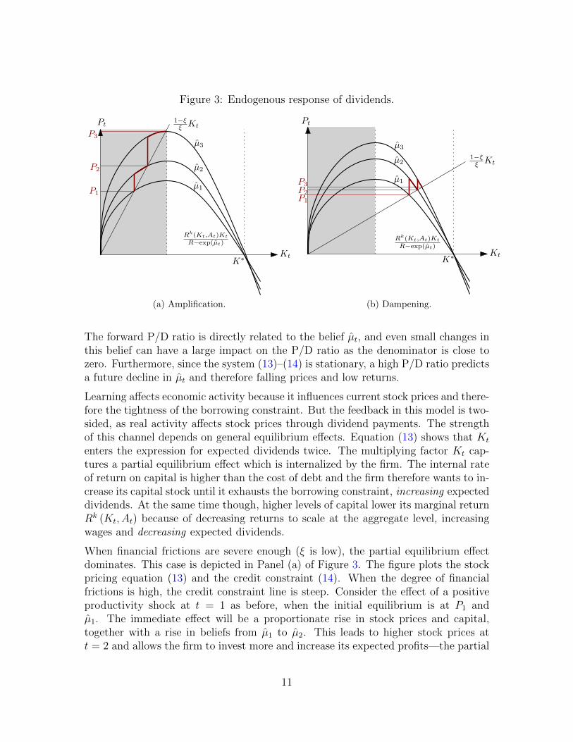
Figure 3: Endogenous response of dividends.
Kt
1−ξξ
Kt
Rk(Kt;At)Kt
R−exp(µt)
µ1
µ2
µ3
K∗
P1
P2
P3
Pt
(a) Amplification.
Kt
1−ξξ
Kt
Rk(Kt;At)Kt
R−exp(µt)
µ1
µ2
µ3
K∗
P1
P2
P3
Pt
(b) Dampening.
The forward P/D ratio is directly related to the belief µt, and even small changes inthis belief can have a large impact on the P/D ratio as the denominator is close tozero. Furthermore, since the system (13)–(14) is stationary, a high P/D ratio predictsa future decline in µt and therefore falling prices and low returns.
Learning affects economic activity because it influences current stock prices and there-fore the tightness of the borrowing constraint. But the feedback in this model is two-sided, as real activity affects stock prices through dividend payments. The strengthof this channel depends on general equilibrium effects. Equation (13) shows that Kt
enters the expression for expected dividends twice. The multiplying factor Kt cap-tures a partial equilibrium effect which is internalized by the firm. The internal rateof return on capital is higher than the cost of debt and the firm therefore wants to in-crease its capital stock until it exhausts the borrowing constraint, increasing expecteddividends. At the same time though, higher levels of capital lower its marginal returnRk (Kt, At) because of decreasing returns to scale at the aggregate level, increasingwages and decreasing expected dividends.
When financial frictions are severe enough (ξ is low), the partial equilibrium effectdominates. This case is depicted in Panel (a) of Figure 3. The figure plots the stockpricing equation (13) and the credit constraint (14). When the degree of financialfrictions is high, the credit constraint line is steep. Consider the effect of a positiveproductivity shock at t = 1 as before, when the initial equilibrium is at P1 andµ1. The immediate effect will be a proportionate rise in stock prices and capital,together with a rise in beliefs from µ1 to µ2. This leads to higher stock prices att = 2 and allows the firm to invest more and increase its expected profits—the partial
11
equilibrium effect dominates. This adds to the rise in realized stock prices, furtherrelaxing the borrowing constraint and increasing next period’s beliefs. Stock prices,investment, and output all rise more than proportionally to productivity.
In Panel (b), credit constraints are not very severe (ξ is large) and the credit constraintline is relatively flat. A relaxation of the borrowing constraint due to a rise in µ2 stillallows the firm to invest and produce more, but in general equilibrium wages rise by somuch that dividends fall. This response of dividends dampens rather than amplifiesthe dynamics of investment and asset prices.
This dampening effect can be so strong as to eliminate the effects of learning alto-gether. The appendix shows that in the limit of vanishing financial frictions, stockprices become a pure random walk again:
logPt − logPt−1ξ→1−→ εt.
As a consequence, the entire dynamics of the model become identical to those underrational expectations. As financial frictions disappear, the general equilibrium effectsoffset any dynamics from stock price learning. This shows that sizable amplifica-tion arises neither from learning nor from credit frictions alone, but only from theirinteraction.
3 Full model for quantitative analysis
This section embeds the mechanism discussed so far into a quantitative New-Keynesianmodel with a financial accelerator. Compared with the simple model in the previ-ous section, I introduce a number of additional elements. First, firms are allowed tofinance capital out of retained earnings. Second, the borrowing constraint is general-ized and microfounded by a limited commitment problem. Third, I add investmentadjustment costs and nominal rigidities. The former improve the quantitative fit,while the latter help to attenuate the general equilibrium effects discussed above.
3.1 Model setup
The economy is closed and operates in discrete time. It is populated by two types ofhouseholds. Lending households consume final goods and supply labor. They tradedebt claims on intermediate goods producers and receive interest from them. Firmowners only consume final goods. They trade equity claims on intermediate goodsproducers and receive dividends from them.
The two households own four types of firms. Only the first type is substantial to themodel analysis: Intermediate goods producers (or simply firms) combine capital and
12
differentiated labor to produce a homogeneous intermediate good. They are ownedby the firm owners, borrow funds from households, and are financially constrained.The other three types of firms serve only to add nominal rigidities and adjustmentcosts to the model. They are owned by the households. Labor agencies transformhomogeneous household labor into differentiated labor services, which they sell tointermediate goods producers. Final good producers transform intermediate goodsinto differentiated final goods. Capital goods producers produce new capital goodsfrom final consumption goods subject to an investment adjustment cost.
Finally, there is a fiscal authority setting tax rates to offset steady-state distortionsfrom monopolistic competition, and a monetary authority setting nominal interestrates. Most elements of the model are standardand their desription is relegated tothe appendix.
3.1.1 Households
A representative household with time-separable preferences maximizes utility as fol-lows:
max(Ct,Lt,Bjt,Bgt )
∞t=0
EP0∞∑t=0
βt log (Ct)− ηL1+φt
1 + φ
s.t. Ct = wtLt +Bgt − (1 + it−1)
pt−1
ptBgt−1 +
ˆ 1
0
(Bjt −Rjt−1Bjt−1) dj + Πt
Here, wt is the real wage received by the household and Lt is the amount of laborsupplied. Bg
t are real quantities of nominal one-period government bonds (in zero netsupply) that pay a nominal interest rate it and pt is the price level, defined below.Households also lend funds Bjt to intermediate goods producers indexed by j ∈ [0, 1]at the real interest rate Rjt. These loans are the outcome of a contracting problemdescribed later on. Πt represents lump-sum profits and taxes. Consumption Ct is itselfa composite CES utility flow from a variety of differentiated goods with elasticity ofsubstitution σ.
The first-order conditions of the household are standard. In what follows I define thestochastic discount factor of the household as Λt+1 = βCt/Ct+1.
3.1.2 Intermediate good producers (firms)
The production of intermediate goods is carried out by a continuum of firms, indexedj ∈ [0, 1]. Firm j enters period t with capital Kjt−1 and a stock of debt Bjt−1 whichneeds to be repaid at the gross real interest rate Rjt−1. First, capital is combinedwith a labor index Ljt to produce output:
Yjt = (Kjt−1)α (AtLjt)1−α , (16)
13

where At is aggregate productivity. The labor index is a CES combination of differ-entiated labor services with elasticity of substitution σw, but the firm’s problem canbe treated as if the labor index was acquired in a competitive market at the real wageindex wt. Output is sold competitively to final good producers at price qt. Duringproduction, the capital stock depreciates at rate δ. This depreciated capital can betraded by the firm at the price Qt.
The firm’s net worth is the difference between the value of its assets and its outstand-ing debt:
Njt = qtYjt − wtLjt +Qt (1− δ)Kjt−1 −Rjt−1Bjt−1. (17)
I assume that the firm exits with probability γ. This probability is exogenous andindependent across time and firms. As in Bernanke, Gertler and Gilchrist (1999), exitprevents firms from becoming financially unconstrained. If a firm does not exit, itneeds to pay out a fraction ζ ∈ (0, 1) of its earnings as dividends (where earnings Ejtare given by Njt−QtKjt−1 +Bjt−1). The number ζ therefore represents the dividendpayout ratio for continuing firms.5 If a firm does exit, it must pay out its entire networth as dividends. It is subsequently replaced by a new firm, which receives theindex j. I assume that this new firm gets endowed with a fixed number of shares,normalized to one, and is able to raise an initial amount of net worth. This amountequals ω (Nt − ζEt), where ω ∈ (0, 1) and Nt and Et are aggregate net worth andearnings, respectively.6
The net worth of firm j after equity changes, entry and exit is given by
Njt =
{Njt − ζEjt for continuing firms,
ω (Nt − ζEt) for new firms.
This firm then decides on the new stock of debt Bjt and the new capital stock Kjt,maximizing the present discounted value of dividend payments using the discountfactor of its owners. Its balance sheet must satisfy:
QtKjt = Bjt + Ntj. (18)
3.1.3 Firm owners
Firm owners differ from households in their capacity to own intermediate firms. Therepresentative firm owner is risk-neutral. It can buy shares in firms indexed by j ∈
5The optimal dividend payout ratio in this model would be ζ = 0, as firms would always preferto build up net worth to escape the borrowing constraint over paying out dividends. However,this would imply that aggregate dividends would be proportional to aggregate net worth, which israther slow-moving. The resulting dividend process would not be nearly as volatile as in the data.Imposing ζ > 0 allows to better match the volatility of dividends and therefore obtain better assetprice properties.
6The simplified firm problem of Section 2 is nested as the caseζ = 1 and γ = 0.
14

[0, 1]. As described above, when a firm exits, it pays out its net worth Njt as dividends,and is replaced by a new firm, which raises equity ω (Nt − ζEt). Let the set of exitingfirms in each period t be denoted by Γt ⊂ [0, 1]. Then, the firm owner’s utilitymaximization problem is given by:
max(Cft ,S
jt )∞t=0
EP0∞∑t=0
βtCft
s.t. Cft +
ˆ 1
0
SjtPjtdj =
ˆj /∈Γt
Sjt−1 (Pjt +Djt) dj (19)
+
ˆj∈Γt
[Sjt−1Djt − ω (Nt − ζEt) + Pjt] dj (20)
Sjt ∈[0, S
](21)
for some S > 1. Firm owners’ consumption Cft is the same aggregator of differentiated
final goods as for households.
The first term on the right-hand side of the budget constraint deals with continuingfirms and is standard: Each share in firm j pays dividends Djt and continues to trade,at price Pjt. The second term deals with firm entry and exit. If the household owns ashare in the exiting firm j, it receives a terminal dividend. At the same time, a newfirm j appears that is able to raise a limited amount of equity ω (Nt − ζEt) from thefirm owner in exchange for a unit amount of shares that can be traded at price Pjt.In addition, firm owners face upper and lower bounds on traded stock holdings.7 Thefirst-order conditions of the firm owner are
Sjt
= 0 if Pjt > βEPt
[Djt+1 + Pjt+11{j /∈Γt+1}
]∈[0, S
]if Pjt = βEPt
[Djt+1 + Pjt+11{j /∈Γt+1}
].
= S if Pjt < βEPt[Djt+1 + Pjt+11{j /∈Γt+1}
] (22)
3.1.4 Borrowing constraint
In choosing their debt holdings, firms are subject to a borrowing constraint. Theconstraint is the solution to a particular limited commitment problem in which theoutside option for the lender in the event of default depends on equity valuations.
Each period, lenders (households) and borrowers (firms) meet to decide on the lendingof funds. Pairings are anonymous. Contracts are incomplete because the repaymentof loans cannot be made contingent. Only the size Bjt and the interest rate Rjt of the
7This renders demand for stocks finite under arbitrary beliefs. In equilibrium, the bounds arenever binding.
15

loan can be contracted in period t. Both the lender (a household) and the firm haveto agree on a contract (Bjt, Rjt). Moreover, there is limited commitment in the sensethat at the end of the period, but before the realization of next period’s shocks, firmj can always choose to enter a state of default. In this case, the value of the debtrepayment must be renegotiated. If the negotiations are successful, then wealth iseffectively shifted from creditors to debtors. The outside option of this renegotiationprocess is bankruptcy of the firm and seizure by the lender.
Bankruptcy carries a cost of a fraction 1−ξ of the firm’s capital being destroyed. Thelender, a household, does not have the ability to operate the firm. It can liquidatethe firm’s assets, selling the remaining capital in the next period. This results ina recovery value of ξQt+1Kjt. With some probability x (independent across timeand firms), the lender receives the opportunity to “restructure” the firm if it wants.Restructuring means that, similar to Chapter 11 bankruptcy proceedings, the firmgets partial debt relief but remains operational. I assume that the lender has tosell the firm to another firm owner, retaining a fraction ξ of the initial debt. Inequilibrium, the recovery value in this case will be ξ (Pjt +Bjt) and this will alwaysbe higher than the recovery value after liquidation. The appendix shows that thedebt contract takes the form of a leverage constraint in which total firm value is aweighted average of liquidation and market value:
Bjt ≤ ξ
(1− x)EPt Λt+1Qt+1ξKjt︸ ︷︷ ︸liquidation value
+x (Pjt +Bjt)︸ ︷︷ ︸market value
(23)
This borrowing constraint nests the one in the simple model for x = 1.
3.1.5 Further model elements and shocks
Investment is subject to quadratic adjustment costs that move the price for capitalgoods:
Qt = 1 + ψ
(ItIt−1
− 1
)(24)
Further, the prices for final goods and wages are subject to Calvo rigidities, with pricestickiness parameter κ and wage stickiness parameter κw. The price for intermediategoods qt equals the inverse of the gross markup of final goods producers. The mon-etary authority setting the nominal interest rate according to a Taylor-type interestrate rule:
it = ρiit−1 + (1− ρi)(β−1 + φππt + εit
), (25)
16

where φπ is the reaction coefficient on consumer price inflation πt, ρi is the degreeof interest rate smoothing, and εit is an interest rate shock. Details of the modelstructure are provided in the appendix.
Finally, the exogenous stochastic processes are productivity and the monetary policyshock:
logAt = (1− ρ) log A+ ρ logAt−1 + log εAt (26)
εAt ∼ iidN(0, σ2
A
)(27)
εit ∼ iidN(0, σ2
i
)(28)
3.2 Rational expectations equilibrium
I first describe the equilibrium under rational expectations. An equilibrium is a setof stochastic processes for prices and allocations, a set of strategies in the limitedcommitment game, and an expectation measure P such that the following holds forall states and time periods: Markets clear; allocations solve the optimization programsof all agents given prices and expectations P ; the strategies in the limited commitmentgame are a subgame-perfect Nash equilibrium for all lender-borrower pairs; and themeasure P satisfies rational expectations.
Under a mild restriction on the exit probability γ, there exists a rational expectationsequilibrium characterized by the following properties.
1. All firms choose the same capital-labor ratio Kjt/Ljt. This allows one to definean aggregate production function and an internal rate of return on capital:
Yt = αKαt−1
(AtLt
)1−α(29)
Rkt = qtα
YtKt−1
+Qt (1− δ)Kt−1 (30)
2. The expected return on capital is higher than the internal return on debt:EtRk
t+1 > Rjt.
3. At any time t, the stock market valuation Pjt of a firm j is proportional to itsnet worth after entry and exit Njt. This permits one to write an aggregate stockmarket index as
Pt =
ˆ 1
0
Pjt = βEt[Dt+1 +
1− γ1− γ + γω
Pt+1
]. (31)
4. Borrowers never default on the equilibrium path and borrow at the risk-freerate
Rjt = Rt =1
EtΛt+1
. (32)
17

The lender only accepts debt payments up to the limit given by (23), whichis proportional to the firm’s net worth Njt, and the firm always exhausts thislimit.
5. As a consequence of the previous properties of the equilibrium, all firms can beaggregated. Aggregate debt, capital, and net worth are sufficient to describethe intermediate goods sector:
Nt = RktKt−1 −Rt−1Bt−1 (33)
QtKt = (1− γ + γω) ((1− ζ)Nt + ζ (Bt−1 −QtKt−1)) +Bt (34)
Bt = xEtΛt+1Qt+1ξKt + (1− x) ξ (Pt +Bt) . (35)
Proofs are relegated to the appendix.
3.3 Learning equilibrium
I introduce learning about stock prices as in the simple model of Section 2. Under thesubjective belief measure P , agents are assumed to retain the belief that the value ofan individual firm is proportional to its net worth, as under rational expectations:
Pjt =Njt
Nt
PtP-almost surely. (36)
But while investors have the correct belief of the cross-section of prices given theaggregate market value, they are uncertain about the evolution of the aggregatevalue Pt itself. I construct the belief system as in the simplified model: Under P , i)agents have the correct belief about the exogenous shocks, ii) agents believe that thestock price Pt evolves according to Equations (9)-(11), iii) agents have conditionallymodel-consistent expectations with respect to stock prices, as defined in Section 2.3.
In practice, I solve the model using a two-stage procedure. The first stage is to solvefor the policy functions and beliefs under P . The Kalman filtering equations thatdescribe beliefs about stock prices are as follows:
logPt = logPt−1 + µt−1 −σ2ν + σ2
η
2+ zt (37)
µt = µt−1 −σ2ν
2+ gzt, (38)
where µt is the mean belief about the trend in stock price growth, and zt is the forecasterror. Under the subjective beliefs P , zt is normally distributed white noise. I imposethat beliefs about any other endogenous variable are consistent with model outcomesconditional on the evolution of stock prices, and so beliefs and policy functions can becalculated using the belief equations about stock prices and the remaining equilibrium
18

equations, taking zt as an exogenous shock process. The market clearing condition forstocks and consumption goods, however, do not enter this first stage of the problem.Adding either one would effectively impose that beliefs about stock prices, too, beconsistent with equilibrium outcomes, thereby falling back to rational expectations.Now, if yt is the set of model variables and ut the set of exogenous shocks, solvingthis first stage leads to the subjective policy function yt = h (yt−1, ut, zt) satisfyingconditionally model-consistent expectations.
The second stage of the model consists in finding the value for zt which leads tomarket clearing in the stock market and thereby establishes equilibrium. This resultsin a mapping from the state variables and exogenous shocks to the perceived forecasterror r : (yt−1, ut) 7→ zt. The resulting process for zt is clearly not an iid disturbance,and in this respect agents’ subjective beliefs are misspecified. The final solution ofthe model is given by the policy function yt = g (yt−1, ut) = h (yt−1, ut, r (yt−1, ut)). Iapproximate the policy functions using a second-order perturbation method.
4 Results
I now present the quantitative results of this paper. First, I discuss the choice ofparameters. Then, I review standard business cycle statistics. Learning and assetprice volatility account for a third of the volatility of output, pointing to the strengthof the endogenous amplification mechanism. I then look at asset pricing momentsand find that the model with learning closely matches the volatility of stock prices(which is targeted by the estimation), but also the predictability of stock returns,skewness and kurtosis. Next, I present impulse response functions, confirming thestrong amplification mechanism. The main channel is the endogenous volatility ofasset prices induced by learning. But I also show that this is not the only channelthrough which learning affects the economy: Expectations about asset prices alsocause procyclical movements in aggregate demand, leading to additional amplificationin the presence of nominal rigidities. Finally, I compare forecast errors made by agentsin the model with those observed in survey data. The patterns of predictability areremarkably similar, lending credibility to the assumed expectation formation process.
4.1 Choice of parameters
I partition the set of parameters into two groups. The first set of parameters is cali-brated to first-order moments, and the second set is estimated by simulated methodof moments (SMM) on second-order moments of US quarterly data.
19

4.1.1 Calibration
The capital share in production is set to α = 0.33, implying a labor share in outputof two thirds. The depreciation rate δ = 0.025 corresponds to 10 percent annualdepreciation. The persistence of the temporary component of productivity is set to0.95.
The discount factor is set such that the steady-state interest rate matches the averageannual real return on Treasury bills of 2.5 percent, implying a discount factor β =0.9938. The elasticity of substitution between varieties of the final consumption good,as well as that among varieties of labor used in production, is set to σ = σw = 4. TheFrisch elasticity of labor supply is set to 3, implying φ = 0.33.
The strength of monetary policy reaction to inflation is set to φπ = 1.5, and thedegree of nominal rate smoothing is set to ρi = 0.85.
Four parameters describe the structure of financial constraints: x, the probabilityof restructuring after default; ξ, the tightness of the borrowing constraint; ω, theequity received by new firms relative to average equity; and γ, the rate of firm exitand entry. I calibrate the restructuring rate to x = 0.093. This is the fraction ofUS business bankruptcy filings in 2006 that filed for Chapter 11 instead of Chapter7, and that subsequently emerged from bankruptcy with an approved restructuringplan (a sensitivity check is included in Section 5.2).8 The remaining three parametersare chosen such that the non-stochastic steady state of the model jointly matches theUS average investment share in output of 20 percent, average debt-to-equity ratio of1:1 (as recorded in the Fed flow of funds), and average quarterly P/D ratio of 139(taken from the S&P500). The parameter values thus are γ = 0.0165, ξ = 0.4152,and ω = 0.018.
4.1.2 Estimation
The remaining parameters are the standard deviations of the technology and mone-tary shocks (σA, σi), the degree of nominal price and wage rigidities (κ, κw), the sizeof investment adjustment costs (ψ), the fraction of dividends paid out as earningsby continuing firms (ζ), and the learning gain (g). I estimate these six parametersto minimize the distance to a set of eight moments pertaining to both business cycleand asset price statistics: The standard deviation of output; the standard deviationsof consumption, investment hours worked, and stock prices relative to output; andthe standard deviations of inflation, the nominal interest rate, and stock returns (see
82006 is the only year for which this number can be constructed from publicly availabledata. Data on bankruptcies by chapter are available at http://www.uscourts.gov/Statistics/
BankruptcyStatistics.aspx. Data on Chapter 11 outcomes are analyzed in various samples byFlynn and Crewson (2009), Warren and Westbrook (2009), Lawton (2012), and Altman (2014).
20
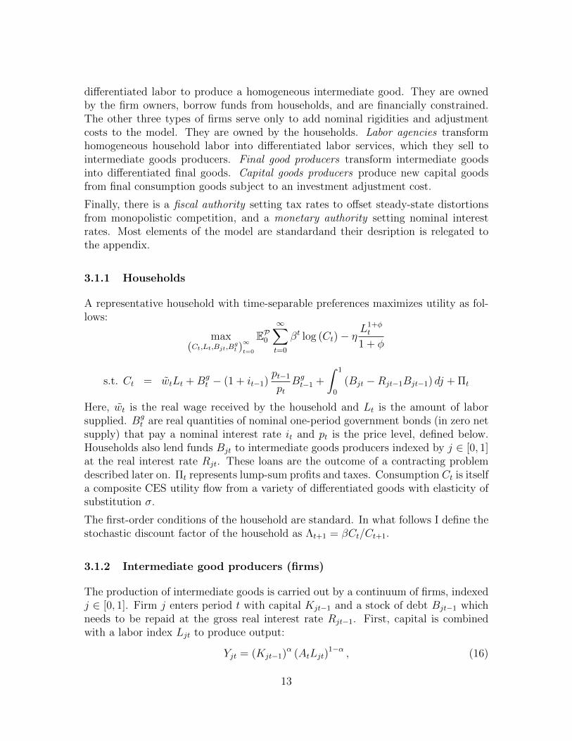
Table 1: Estimated parameters.
param. σa σi κ κw ψ ζ g
learning .00884 .000423 .546 .932 13.7 .632 .00563
(.000967) (.00195) (.089) (.132) (3.85) (.0935) (.000334)
RE .0114 .000895 .691 .572 .618 .0490 -
(.00212) (.00173) (.168) (2.73) (10.7) (11.3)
fric.less .0116 .00121 .671 .847 .558 - -
(.00716) (.000701) (.261) (.398) (.124)Parameters as estimated by simulated method of moments. Asymptotic standard errors in paren-theses.
also Table 2). The set of estimated parameters θ solves
minϑ∈A
(m (θ)− m)′W (m (θ)− m)′ ,
where m (θ) are moments obtained from model simulation paths with 50,000 periods,m are the estimated moments in the data, and W is a weighting matrix.9 I also imposethat θ has to lie in a subset A of the parameter space which rules out deterministicoscillations of stock prices.10 Such oscillations are not observed in the data, but canbe consistent with equilibrium when asset price volatility is high and subjective beliefsare far away from rational expectations. In a sense, this restriction constrains thedegree of departure of subjective beliefs from rational expectations.
Table 1 summarizes the SMM estimates for both the learning and rational expecta-tions version of the model, as well as for a comparison (rational expectations) modelin which all financial frictions are eliminated. The first row presents the results un-der learning. Exogenous shocks come mainly from productivity shocks, since σi isestimated to be relatively small. The Calvo price adjustment parameter is set toκ = 0.546, implying retailers adjust their prices every two quarters. The SMM pro-cedure selects a high degree of nominal wage rigidities κw and of adjustment costs ψ.The estimates are substantially larger than what is commonly found in the literature.The fraction of earnings paid out as dividends is fitted to ζ = 0.632, which is in linewith the historical average for the S&P500 at about 50 percent. Finally, the learninggain g = 0.00563 implies that agents believe the degree of predictability in the stockmarket to be very small.
The second row contains the parameters estimated under rational expectations. Thefit of the asset price moments is worse and the asymptotic standard errors are large,
9I choose W = diag(
Σ)−1
where Σ is the covariance matrix of the data moments, estimated
using a Newey-West kernel with optimal lag order. This choice of W leads to a consistent estimatorthat places more weight on moments which are more precisely estimated in the data.
10θ /∈ A iff there exists an impulse response of stock prices with positive peak value also having anegative value of more than 20% of the peak value.
21
implying that the distance of the moments to the data at the point estimate is rel-atively flat. Nevertheless, at the point estimate, the size of the shocks σa and σiis substantially larger under learning. This implies that learning about stock pricesleads to substantial amplification of shocks: The increased endogenous volatility ofasset prices greatly magnifies the financial accelerator effect, just as in the simplemodel of Section 2. The degree of wage rigidities and investment adjustment costsrequired to fit the data is smaller than under learning.
The third row contains parameter estimates under rational expectations when addi-tionally, financial frictions are completely shut off. Since the financial structure iseliminated from that model, the dividend payout ratio ζ is not present. The sizeof the shocks is larger than under the rational expectations model with the financialaccelerator present. This points to moderate amplification effects of financial frictionsunder rational expectations.
4.2 Business cycle and asset price moments
To get a better understanding of the quantitative properties of the model, I reviewkey moments in the data and across model specifications. Table 2 starts with businesscycle statistics. The moments in the data are shown in Column (1). Moments forthe estimated learning model are shown in Column (2), while Columns (3) and (4)contain the corresponding moments for the model under rational expectations andthe frictionless benchmark. Here, the parameters are held constant at the estimatedvalues as for the learning model. By nature of the estimation, the learning modelhas the best fit across Columns (2) to (4). The comparison serves to single out thecontribution of learning and financial frictions to the fit. Column (5) presents themoments under rational expectations when the parameters are re-estimated to fit thedata.
The first row reports the standard deviation of detrended output. By construction,this is matched well by the learning model in Column (2). When learning is shut offin Column (2), the standard deviation drops one-third. This shows the great degreeof amplification that learning adds to the model. Of course, it is possible to matchoutput volatility with rational expectations, using larger shock sizes, as in Column(5). But the comparison between Columns (2) and (3) singles out the contributionof learning to the internal amplification mechanism. The standard (rational expec-tations) financial accelerator mechanism is present in the model as well, since thevolatility of output drops further in Column (4) when financial frictions are shut off.
The next three rows report the standard deviation of consumption, investment, andhours worked relative to output. Moving from Column (2) to (3), it can be seenthat the removal of learning leads to a sharp drop in the relative volatility of bothinvestment and hours worked. This is because the estimated learning model features
22
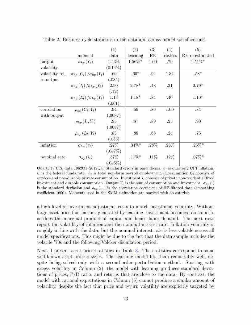
Table 2: Business cycle statistics in the data and across model specifications.
(1) (2) (3) (4) (5)
moment data learning RE fric.less RE re-estimated
output
volatility
σhp (Yt) 1.43%
(0.14%)
1.56%* 1.00 .79 1.51%*
volatility rel.
to output
σhp (Ct) /σhp (Yt) .60
(.035)
.60* .94 1.34 .58*
σhp (It) /σhp (Yt) 2.90
(.12)
2.78* .48 .31 2.79*
σhp (Lt) /σhp (Yt) 1.13
(.061)
1.18* .84 .40 1.10*
correlation
with output
ρhp (Ct, Yt) .94
(.0087)
.59 .86 1.00 .84
ρhp (It, Yt) .95
(.0087)
.87 .89 .25 .90
ρhp (Lt, Yt) .85
(.035)
.88 .65 .24 .76
inflation σhp (πt) .27%
(.047%)
.34%* .28% .28% .25%*
nominal rate σhp (it) .37%
(.046%)
.11%* .11% .12% .07%*
Quarterly U.S. data 1962Q1–2012Q4. Standard errors in parentheses. πt is quarterly CPI inflation.it is the federal funds rate. Lt is total non-farm payroll employment. Consumption Ct consists ofservices and non-durable private consumption. Investment It consists of private non-residential fixedinvestment and durable consumption. Output Yt is the sum of consumption and investment. σhp (·)is the standard deviation and ρhp (·, ·) is the correlation coefficient of HP-filtered data (smoothingcoefficient 1600). Moments used in the SMM estimation are marked with an asterisk.
a high level of investment adjustment costs to match investment volatility. Withoutlarge asset price fluctuations generated by learning, investment becomes too smooth,as does the marginal product of capital and hence labor demand. The next rowsreport the volatility of inflation and the nominal interest rate. Inflation volatility isroughly in line with the data, but the nominal interest rate is less volatile across allmodel specifications. This might be due to the fact that the data sample includes thevolatile ’70s and the following Volcker disinflation period.
Next, I present asset price statistics in Table 3. The statistics correspond to somewell-known asset price puzzles. The learning model fits them remarkably well, de-spite being solved only with a second-order perturbation method. Starting withexcess volatility in Column (2), the model with learning produces standard devia-tions of prices, P/D ratio, and returns that are close to the data. By contrast, themodel with rational expectations in Column (5) cannot produce a similar amount ofvolatility, despite the fact that price and return volatility are explicitly targeted by
23
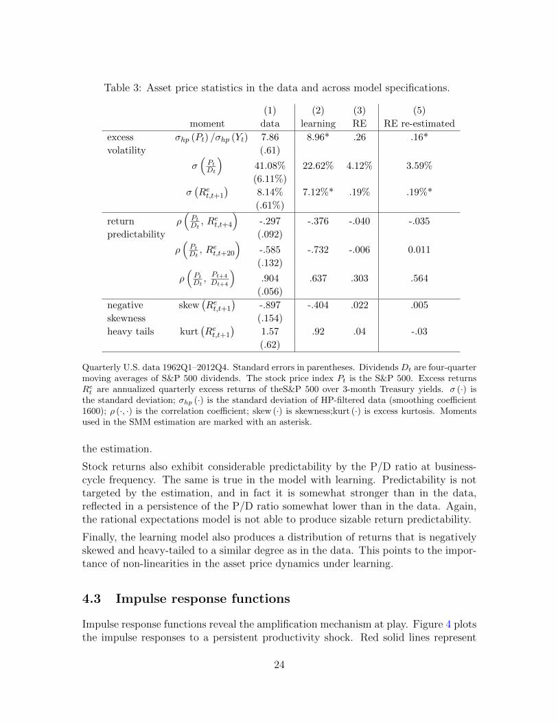
Table 3: Asset price statistics in the data and across model specifications.
(1) (2) (3) (5)
moment data learning RE RE re-estimated
excess
volatility
σhp (Pt) /σhp (Yt) 7.86
(.61)
8.96* .26 .16*
σ(PtDt
)41.08%
(6.11%)
22.62% 4.12% 3.59%
σ(Ret,t+1
)8.14%
(.61%)
7.12%* .19% .19%*
return
predictability
ρ(PtDt, Ret,t+4
)-.297
(.092)
-.376 -.040 -.035
ρ(PtDt, Ret,t+20
)-.585
(.132)
-.732 -.006 0.011
ρ(PtDt, Pt+4
Dt+4
).904
(.056)
.637 .303 .564
negative
skewness
skew(Ret,t+1
)-.897
(.154)
-.404 .022 .005
heavy tails kurt(Ret,t+1
)1.57
(.62)
.92 .04 -.03
Quarterly U.S. data 1962Q1–2012Q4. Standard errors in parentheses. Dividends Dt are four-quartermoving averages of S&P 500 dividends. The stock price index Pt is the S&P 500. Excess returnsRe
t are annualized quarterly excess returns of theS&P 500 over 3-month Treasury yields. σ (·) isthe standard deviation; σhp (·) is the standard deviation of HP-filtered data (smoothing coefficient1600); ρ (·, ·) is the correlation coefficient; skew (·) is skewness;kurt (·) is excess kurtosis. Momentsused in the SMM estimation are marked with an asterisk.
the estimation.
Stock returns also exhibit considerable predictability by the P/D ratio at business-cycle frequency. The same is true in the model with learning. Predictability is nottargeted by the estimation, and in fact it is somewhat stronger than in the data,reflected in a persistence of the P/D ratio somewhat lower than in the data. Again,the rational expectations model is not able to produce sizable return predictability.
Finally, the learning model also produces a distribution of returns that is negativelyskewed and heavy-tailed to a similar degree as in the data. This points to the impor-tance of non-linearities in the asset price dynamics under learning.
4.3 Impulse response functions
Impulse response functions reveal the amplification mechanism at play. Figure 4 plotsthe impulse responses to a persistent productivity shock. Red solid lines represent
24
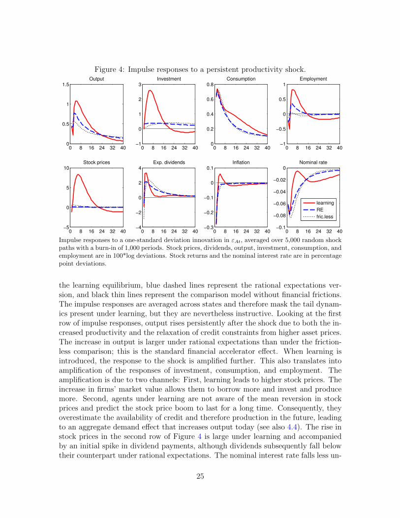
Figure 4: Impulse responses to a persistent productivity shock.
0 8 16 24 32 400
0.5
1
1.5Output
0 8 16 24 32 40−1
0
1
2
3Investment
0 8 16 24 32 400
0.2
0.4
0.6
0.8Consumption
0 8 16 24 32 40−1
−0.5
0
0.5
1Employment
0 8 16 24 32 40−5
0
5
10Stock prices
0 8 16 24 32 40−4
−2
0
2
4Exp. dividends
0 8 16 24 32 40−0.3
−0.2
−0.1
0
0.1Inflation
0 8 16 24 32 40−0.1
−0.08
−0.06
−0.04
−0.02
0Nominal rate
learning
RE
fric.less
Impulse responses to a one-standard deviation innovation in εAt, averaged over 5,000 random shockpaths with a burn-in of 1,000 periods. Stock prices, dividends, output, investment, consumption, andemployment are in 100*log deviations. Stock returns and the nominal interest rate are in percentagepoint deviations.
the learning equilibrium, blue dashed lines represent the rational expectations ver-sion, and black thin lines represent the comparison model without financial frictions.The impulse responses are averaged across states and therefore mask the tail dynam-ics present under learning, but they are nevertheless instructive. Looking at the firstrow of impulse responses, output rises persistently after the shock due to both the in-creased productivity and the relaxation of credit constraints from higher asset prices.The increase in output is larger under rational expectations than under the friction-less comparison; this is the standard financial accelerator effect. When learning isintroduced, the response to the shock is amplified further. This also translates intoamplification of the responses of investment, consumption, and employment. Theamplification is due to two channels: First, learning leads to higher stock prices. Theincrease in firms’ market value allows them to borrow more and invest and producemore. Second, agents under learning are not aware of the mean reversion in stockprices and predict the stock price boom to last for a long time. Consequently, theyoverestimate the availability of credit and therefore production in the future, leadingto an aggregate demand effect that increases output today (see also 4.4). The rise instock prices in the second row of Figure 4 is large under learning and accompaniedby an initial spike in dividend payments, although dividends subsequently fall belowtheir counterpart under rational expectations. The nominal interest rate falls less un-
25

Figure 5: Impulse responses to a monetary shock.
0 8 16 24 32 400
0.2
0.4
0.6
0.8Output
0 8 16 24 32 40−0.5
0
0.5
1
1.5Investment
0 8 16 24 32 400
0.05
0.1
0.15
0.2
0.25Consumption
0 8 16 24 32 40−0.5
0
0.5
1Employment
0 8 16 24 32 40−1
0
1
2
3
4Stock prices
0 8 16 24 32 40−1
0
1
2
3
4Exp. dividends
0 8 16 24 32 40−0.05
0
0.05
0.1
0.15Inflation
0 8 16 24 32 40−0.04
−0.03
−0.02
−0.01
0
0.01Nominal rate
learning
RE
fric.less
Impulse responses to a innovation in εmt, averaged over 5,000 random shock paths with a burn-in of1,000 periods. The size of the innovation is chosen to produce a 10 basis point fall in the equilibriumnominal rate. Stock prices, dividends, output, investment, consumption and employment are in100*log deviations. Stock returns and the nominal interest rate are in percentage point deviations.
der learning as the monetary authority reacts to the inflationary pressures stemmingfrom the relaxation in credit constraints.
Figure 5 plots the response to a temporary reduction in the nominal interest rate.Again, all macroeconomic aggregates rise substantially more under learning thanunder both rational expectations and the frictionless benchmark. The monetarystimulus increases stock prices and thus relaxes credit constraints. The consequentincrease in aggregate demand raises inflationary pressure, so that the systematicreaction of the interest rate rule raises the interest rate sharply again after the shock.
4.4 Does learning matter?
The discussion so far has mainly focused on how large swings in asset prices lead tolarge swings in real activity through their effect on credit constraints. But is learningnecessary for this story at all? Maybe all that matters for amplification is that assetprice volatility has to be increased, by some mechanism or other. In this section, Ishow that learning has an effect on amplification over and above its effect on assetprices.
26

Figure 6: Does learning matter?
0 10 20 30 40−1
0
1
2
3
4Stock prices P
t / V
t
0 10 20 30 40−0.2
0
0.2
0.4
0.6
0.8Output Y
t
0 10 20 30 40−0.5
0
0.5
1
1.5
2Investment I
t
0 10 20 30 400
0.2
0.4
0.6
0.8Consumption C
t
counterfactual
learning
Solid red line: Impulse response to a one standard deviation positive productivity shock underlearning. Black dash dotted line: Impulse response to a hypothetical rational expectations modelwith stock price dynamics identical to those under learning (see text). The impulse responses in thefigure are produced using a first-order approximation to the model equations.
I replace the stock market value Pt in the borrowing constraint (35) with an exogenousprocess Vt that has the same law of motion as the stock price under learning. Moreprecisely, I fit an ARMA(10,5) process for Vt such that its impulse responses are asclose as possible to those of Pt under learning (the exogenous shock in the ARMAprocess are the productivity and monetary shocks). I then solve this model, butwith rational expectations. If learning only matters because it affects stock pricedynamics, then this hypothetical model should have exactly identical dynamics tothe model under learning.11
Figure 6 shows that this is not the case. The ARMA process fits stock prices well:The impulse response of Pt under learning and Vt in the counterfactual experiment areindistinguishable. But after a positive productivity shock, output, investment, andconsumption rise more under learning, even though the counterfactual model has thesame stock price dynamics by construction. The reason is that expectations of futureasset prices matter beyond their direct impact on current prices. Under learning,agents do not fully internalize mean reversion in stock prices and therefore predict thatcredit constraints are loose for longer than they turn out to be. This leads to a wealtheffect on households that increases their consumption, raising aggregate demand, and
11For this exercise I only compute a first-order approximation to the model equations.
27

Figure 7: Return expectations and expected returns in a model simulation.
2.2
2.4
2.6
2.8
33.
21-
year
ret
urn
fore
cast
3.4 3.6 3.8 4 4.2log P/D ratio
-60
-40
-20
020
4060
1-ye
ar r
ealis
ed r
etur
n
3.4 3.6 3.8 4 4.2log P/D ratio
Expected and realized nominal returns along a simulated path of model with learning. Simulationlength 200 periods. Theoretical correlation coefficient for subjective expected returns ρ = .47, forfuture realized returns ρ = −.38.
it leads to higher future expected prices of capital goods EtQt+1, which enters theliquidation value of firms and hence relaxes borrowing constraints, even if stock pricesare the same as under rational expectations. These effects are powerful enough tocreate significant endogenous amplification through the departure of subjective beliefsfrom rational expectations.
4.5 Relation to survey evidence on expectations
The rational expectations hypothesis asserts that “outcomes do not differ systemat-ically [...] from what people expect them to be” (Sargent, 2008). Put differently, aforecast error should not be systematically predictable by information available atthe time of the forecast. The absence of predictability is almost always rejected inthe data.
Similarly, agents in the model under learning also make systematic, predictable fore-cast errors. This holds not only for stock prices but also other endogenous modelvariables, despite the fact that, conditional on stock prices, agents’ beliefs are model-consistent. A systematic mistake in predicting stock prices will still spill over intoa corresponding mistake in predicting the tightness of credit constraints, and henceinvestment, output, and so forth. Owing to the internal consistency of beliefs, I cancompute well-defined forecast errors made by agents in the model at any horizon andfor any model variable.
Figure 7 repeats the scatter plot of the introduction, contrasting expected and realized
28

Table 4: Forecast errors under learning and in the data.
(1) (2) (3) (4) (5) (6)
logPDt ∆ logPDt forecast revision
forecast variable data model data model data model
Rstockt,t+4 -.44 -.38 .06 .30 - -.30
(-3.42) (.41)
Yt,t+3 -.21 -.16 .22 .16 .29 .28
(-1.78) (2.42) (3.83)
It,t+3 -.20 -.37 .25 .27 .31 .35
(-1.74) (2.88) (3.79)
Ct,t+3 -.19 -.04 .21 .01 .23 .02
(-1.85) (2.37) (2.67)
ut,t+3 .05 .20 -.27 -.20 .43 .32
(.12) (-3.07) (6.07)
Correlation coefficients for mean forecast errors on one year-ahead nominal stock returns (Graham-Harvey survey) and three quarters-ahead real output growth, investment growth, consumptiongrowth and the unemployment rate (SPF). t-statistics in parentheses. Regressors: Column (1)is the S&P 500 P/D ratio and Column (2) is its first difference. Column (3) is the forecast revision,as in Coibion and Gorodnichenko (2015). Data from Graham-Harvey covers 2000Q3–2012Q4. Datafor the SPF covers 1981Q1–2012Q4. For the model, correlations are computed using a simulationof length 50,000, where subjective forecasts are computed using a second-order approximation tothe subjective belief system on a path in which no more future shocks occur, starting at the currentstate in each period. Unemployment in the model is taken to be ut = 1− Lt. Stock returns in themodel Rstock
t,t+4 are quarterly nominal aggregate market returns.
one year-ahead returns in a model simulation. The same pattern as in the dataemerges: When the P/D ratio is high, return expectations are most optimistic. Inthe learning model, this has a causal interpretation: High return expectations driveup stock prices. At the same time, realized future returns are, on average, low whenthe P/D ratio is high. This is because the P/D ratio is mean-reverting (which agentsdo not realize, instead extrapolating past price growth into the future): At the peakof investor optimism, realized price growth is already reversing and expectations aredue to be revised downward, pushing down prices toward their long-run mean.
Table 4 describes tests using the Federal Reserve’s Survey of Professional Forecasters(SPF) as well as the CFO survey data and compares the statistics to those obtainedfrom simulated model data. Each entry corresponds to a correlation of the error ofthe mean survey forecast with a variable that is observable by respondents at thetime of the survey. Under the null of rational expectations, all entries should be zero.
Column (1) shows that the P/D ratio negatively predicts forecast errors. When stockprices are high, people systematically under-predict economic outcomes. This holdsin particular for stock returns, as was already shown in the scatter plot above. But
29

it also holds true for macroeconomic aggregates, albeit at lower levels of significance.The same holds true in Column (2), which shows the correlation coefficients obtainedfrom simulated model data.
Column (3) repeats the exercise for the growth rate of the P/D ratio. This mea-sure positively predicts forecast errors, suggesting that agents’ expectations are toocautious and under-predict an expansion in its beginning but then overshoot and over-predict it when it is about to end. In the model (Column 4), this pattern also emergesbecause expectations about asset prices (and hence lending conditions) adjust onlyslowly. The similarity of the correlations in the data and in the model is striking, withthe exception of aggregate consumption. The reason is that consumption forecasts inthe model are only biased at longer horizons: A relaxation of borrowing constraintsfirst leads to an increase in investment and only later to an increase in consumption.Agents are aware of this relationship, so that their three-quarter forecasts, as in Ta-ble 4 do not become much more optimistic when the P/D ratio increases. At longerforecast horizons, one would observe more predictability for consumption as well.
Column (5) reports the results of a particular test of rational expectations devisedby Coibion and Gorodnichenko (2015). Since for any variable xt, the SPF asks forforecasts at one- through four-quarter horizons, it is possible to construct a measure ofagents’ revision of the change in xt as Et [xt+3 − xt]− Et−1 [xt+3 − xt]. Forecast errorsare positively predicted by this revision measure. Coibion and Gorodnichenko takethis as evidence for sticky information models in which information sets are graduallyupdated over time. But it is also consistent with the learning model: The correlationcoefficients in Column (6) are very similar to those in the data.12
5 Sensitivity checks
5.1 Nominal rigidities
The quantitative model includes price- and wage-setting frictions that complicatethe model dynamics. They are nevertheless important for the quantitative fit of themodel, as I will argue here. Recall that in the simple model of Section 2, the amplify-ing effect of asset price learning depended crucially on the behavior of the real wage.After a positive shock, as credit constraints relax and investment picks up, wages risewhich work to diminish firms’ profits and expected dividend payments. This drivesdown stock prices and dampens the learning dynamics. The same mechanism is at
12The model predicts a negative correlation of forecast errors on stock returns with their forecastrevisions. The CFO survey does not allow for the construction of the corresponding statistic in thedata, but it is an interesting implication since a negative correlation cannot be produced by rigidinformation models as in Coibion and Gorodnichenko.
30
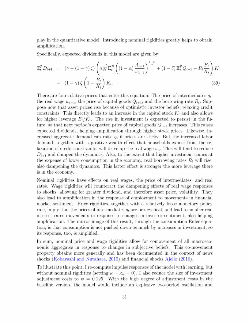
play in the quantitative model. Introducing nominal rigidities greatly helps to obtainamplification.
Specifically, expected dividends in this model are given by:
EPt Dt+1 = (γ + (1− γ) ζ)
(αq
1αt EPt
((1− α)
At+1
wt+1
) 1−αα
+ (1− δ)EPt Qt+1 −RtBt
Kt
)Kt
− (1− γ) ζ
(1− Bt
Kt
)Kt. (39)
There are four relative prices that enter this equation: The price of intermediates qt,the real wage wt+1, the price of capital goods Qt+1, and the borrowing rate Rt. Sup-pose now that asset prices rise because of optimistic investor beliefs, relaxing creditconstraints. This directly leads to an increase in the capital stock Kt and also allowsfor higher leverage Bt/Kt. The rise in investment is expected to persist in the fu-ture, so that next period’s expected price of capital goods Qt+1 increases. This raisesexpected dividends, helping amplification through higher stock prices. Likewise, in-creased aggregate demand can raise qt if prices are sticky. But the increased labordemand, together with a positive wealth effect that households expect from the re-laxation of credit constraints, will drive up the real wage wt. This will tend to reduceDt+1 and dampen the dynamics. Also, to the extent that higher investment comes atthe expense of lower consumption in the economy, real borrowing rates Rt will rise,also dampening the dynamics. This latter effect is stronger the more leverage thereis in the economy.
Nominal rigidities have effects on real wages, the price of intermediates, and realrates. Wage rigidities will counteract the dampening effects of real wage responsesto shocks, allowing for greater dividend, and therefore asset price, volatility. Theyalso lead to amplification in the response of employment to movements in financialmarket sentiment. Price rigidities, together with a relatively loose monetary policyrule, imply that the prices of intermediates qt are pro-cyclical, and lead to smaller realinterest rates movements in response to changes in investor sentiment, also helpingamplification. The mirror image of this result, through the consumption Euler equa-tion, is that consumption is not pushed down as much by increases in investment, soits response, too, is amplified.
In sum, nominal price and wage rigidities allow for comovement of all macroeco-nomic aggregates in response to changes in subjective beliefs. This co-movementproperty obtains more generally and has been documented in the context of newsshocks (Kobayashi and Nutahara, 2010) and financial shocks Ajello (2016).
To illustrate this point, I re-compute impulse responses of the model with learning, butwithout nominal rigidities (setting κ = κw = 0). I also reduce the size of investmentadjustment costs to ψ = 0.125. With the high degree of adjustment costs in thebaseline version, the model would include an explosive two-period oscillation and
31

Figure 8: Role of nominal rigidities.
0 12 24 360
0.5
1
1.5Output
0 12 24 36−1
0
1
2
3Investment
0 12 24 360
0.2
0.4
0.6
0.8Consumption
0 12 24 36−5
0
5
10Stock prices
0 12 24 36−2
0
2
4Exp. dividends
0 12 24 360
0.2
0.4
0.6
0.8Real wage
learning
κ=κw
=0
Solid red line: Impulse response to a one-standard deviation positive productivity shock for themodel with learning and price and wage rigidities (“nominal” baseline). Black dash-dotted line:Impulse response to a productivity shock for the model with learning but without nominal rigidities,re-estimated as in Section 4.1.2 to fit the data (“real” comparison). The size of the shock shown isthe same as in the nominal model.
reducing ψ ensures stability. The low costs of adjusting investment also gives thereal version a better chance at delivering strong impulse responses. Even then, thenominal version delivers far greater amplification. Figure 8 plots impulse responsesto a positive productivity shock for both the nominal and real version of the model.Owing to lower adjustment costs, the initial response of investment is expectedlystronger in the real version. However, the real wage wt rises by much more, and alsothe price of intermediates qt is fixed, so dividends do not rise as much after the shock.This considerably dampens the learning dynamics and mutes the response of stockprices. By consequence, the response of output, investment, consumption and hoursworked (not shown) is overall weaker than in the baseline version of the model.
5.2 Borrowing constraint parameters
I turn to discuss the sensitivity to the two main parameters affecting the borrowingconstraint (35): The probability x that a firm can be sold as a going concern afterfiling for bankruptcy, governing the dependency of the constraint on stock prices; andthe fraction of assets ξ preserved in bankruptcy, governing the overall tightness ofthe constraint. Figure 9 plots the standard deviation of output and stock prices as afunction of these two parameters, respectively.
32

Figure 9: Sensitivity to borrowing constraint parameters.
0 0.05 0.1 0.15 0.2 0.250
5
10
sd
. %
Output
0 0.05 0.1 0.15 0.2 0.250
10
20
30
40
sd
. %
Stock prices
x
(a) Market value dependency x.
0 0.1 0.2 0.3 0.4 0.5 0.6 0.7 0.80
1
2
sd
. %
Output
0 0.1 0.2 0.3 0.4 0.5 0.6 0.7 0.80
5
10
15
sd
. %
Stock prices
ξ
(b) Recovery rate ξ.Simulated model data HP-filtered with smoothing parameter 1600, sample length 50,000 periods.The dashed black lines indicate parameter value in the estimated learning model.
Panel (a) shows the role of the x parameter, which crucially affects the amplifica-tion mechanism. The value x = 0 is a special case. At this point, stock prices donot enter the borrowing constraint and serve no role for allocations in the economy.Allocations under learning and rational expectations coincide perfectly, even thoughstock price dynamics are still amplified under learning. As x increases, the highervolatility of stock prices under learning translates into higher volatility in real activityas well. Since swings in real activity feed back into asset prices through their effecton dividends, the amplification becomes very strong for high values of x until thedynamics become explosive. Beyond a value of x of about 0.26, no stable learningequilibrium exists. By contrast, the rational expectations equilibrium barely dependson the parameter x.
Panel (b) shows the role of the ξ parameter. Amplification is hump-shaped with re-spect to ξ. At ξ = 0, no collateral is pledgeable and firms have to finance their capitalstock entirely out of equity. In this case, fluctuations in stock prices again do not im-pact the economy and allocations coincide under learning and rational expectations;there is no amplification from learning. However, as pledgeability increases to itsmaximum value (beyond which a steady state with permanently binding borrowingconstraint does not exist), amplification also disappears. This mirrors the analysis ofthe simplified model.
5.3 Monetary policy rule
Finally, I discuss the sensitivity of the results with respect to the interest rate rulefollowed by the monetary authority. Consider extending the interest rate rule (25) asfollows:
33

it = ρiit−1 + (1− ρi) (1/β + φππt + φY ∆ log Yt + φP∆ logPt) (40)
In addition to raising interest rates when inflation is above its target level (taken tobe zero), the monetary authority can raise interest rates φ∆Y percentage points whenreal GDP growth increases one percentage point and φ∆P percentage points whenstock price growth increases one percentage point.13 I consider several values forthe parameters φπ, φ∆Y , φ∆P . Table 5 summarizes how they affect the model underlearning. In addition to the standard deviations of output, stock prices, inflationand nominal interest rates, the table also reports a measure of amplification by thelearning dynamics and a measure of the welfare cost of business cycles.14
Column (1) shows the baseline calibration under learning. Learning amplifies outputfluctuations by 33 percent and has a welfare cost of business cycles of 0.0346 percentof average consumption. In Column (2), the coefficient on inflation φπ is doubled.This rule achieves a marked reduction in the volatility of inflation, but at the cost ofhigher output volatility. The amount of amplification from learning is smaller thanin the baseline but still strong at 22 percent. Column (3) augments the baseline ruleby a reaction to output growth. This rule reduces the volatility of output and stockprices, while keeping the volatility of inflation unchanged. Again, the amplificationeffect from learning is dampened but output is still 25 percent more volatile thanunder rational expectations. Column (4) considers a reaction of interest rates tostock price growth. Such a reaction is highly effective in stabilizing the economy underlearning. The volatility of output and stock prices drops markedly. The amplificationmechanism is completely eliminated—output volatility under learning is 10 percentlower than under rational expectations, and the welfare cost of business cycles islower than in Columns (1)–(3). Intuitively, raising rates when asset prices are rising(and vice-versa) acts to stabilize expectations in financial markets. In the model, this
13I deliberately exclude levels or gap measures of output or asset prices from the interest raterule. Doing so would imply that the monetary authority has more knowledge than the private sectorunder learning, as the perceived equilibrium level of asset prices and the output gap depends onagents’ subjective beliefs, and at the same time communicates that knowledge through the rule.
14The amplification measure is the ratio of the standard deviation of output under learning overthat under rational expectations at the same parameter values. The welfare cost of business cycles χis defined as the fraction of steady-state consumption the household would need to give up in orderto have its period utility at the same level as the average stochastic period utility, in a steady statein which consumption and labor are constant and equal to their average stochastic level, and priceand wage dispersion is nil:
u(
(1− χ)E[Ct
],E[Lt
])= E [u (Ct, Lt)] .
I simulate a model time series for (Ct, Lt, πt, πwt ) of 10,000 periods using the second-order approx-
imation method above, and I compute series for Ct and Lt using the exact formulae given in theappendix. I then evaluate period utility using its exact formula as well to calculate the welfare loss.The expectation is then computed using averages over time.
34
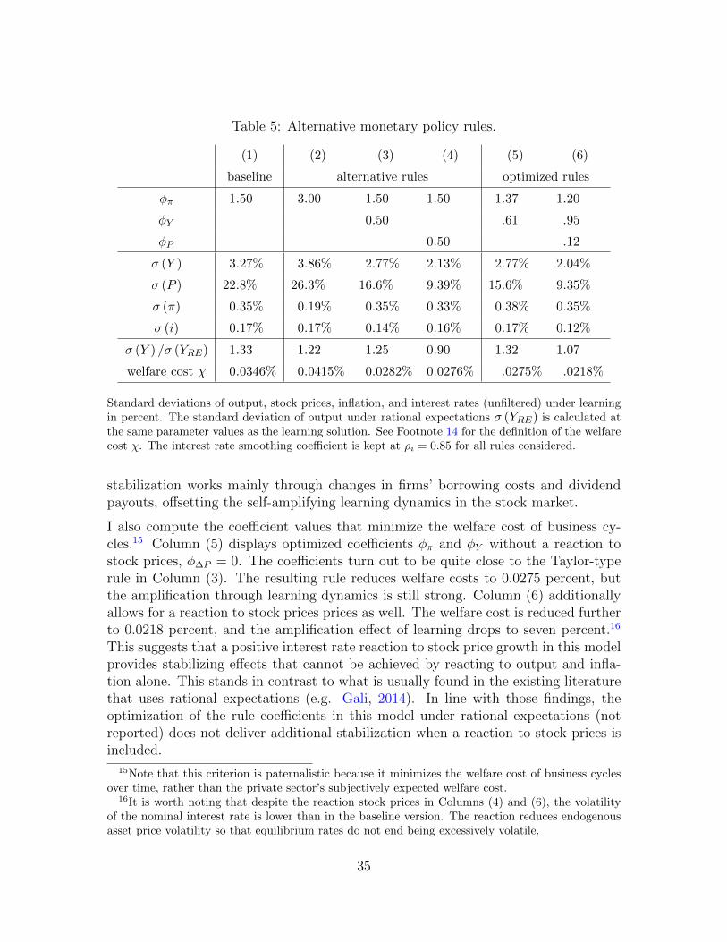
Table 5: Alternative monetary policy rules.
(1) (2) (3) (4) (5) (6)
baseline alternative rules optimized rules
φπ 1.50 3.00 1.50 1.50 1.37 1.20
φY 0.50 .61 .95
φP 0.50 .12
σ (Y ) 3.27% 3.86% 2.77% 2.13% 2.77% 2.04%
σ (P ) 22.8% 26.3% 16.6% 9.39% 15.6% 9.35%
σ (π) 0.35% 0.19% 0.35% 0.33% 0.38% 0.35%
σ (i) 0.17% 0.17% 0.14% 0.16% 0.17% 0.12%
σ (Y ) /σ (YRE) 1.33 1.22 1.25 0.90 1.32 1.07
welfare cost χ 0.0346% 0.0415% 0.0282% 0.0276% .0275% .0218%
Standard deviations of output, stock prices, inflation, and interest rates (unfiltered) under learningin percent. The standard deviation of output under rational expectations σ (YRE) is calculated atthe same parameter values as the learning solution. See Footnote 14 for the definition of the welfarecost χ. The interest rate smoothing coefficient is kept at ρi = 0.85 for all rules considered.
stabilization works mainly through changes in firms’ borrowing costs and dividendpayouts, offsetting the self-amplifying learning dynamics in the stock market.
I also compute the coefficient values that minimize the welfare cost of business cy-cles.15 Column (5) displays optimized coefficients φπ and φY without a reaction tostock prices, φ∆P = 0. The coefficients turn out to be quite close to the Taylor-typerule in Column (3). The resulting rule reduces welfare costs to 0.0275 percent, butthe amplification through learning dynamics is still strong. Column (6) additionallyallows for a reaction to stock prices prices as well. The welfare cost is reduced furtherto 0.0218 percent, and the amplification effect of learning drops to seven percent.16
This suggests that a positive interest rate reaction to stock price growth in this modelprovides stabilizing effects that cannot be achieved by reacting to output and infla-tion alone. This stands in contrast to what is usually found in the existing literaturethat uses rational expectations (e.g. Gali, 2014). In line with those findings, theoptimization of the rule coefficients in this model under rational expectations (notreported) does not deliver additional stabilization when a reaction to stock prices isincluded.
15Note that this criterion is paternalistic because it minimizes the welfare cost of business cyclesover time, rather than the private sector’s subjectively expected welfare cost.
16It is worth noting that despite the reaction stock prices in Columns (4) and (6), the volatilityof the nominal interest rate is lower than in the baseline version. The reaction reduces endogenousasset price volatility so that equilibrium rates do not end being excessively volatile.
35
6 Conclusion
In this paper, I have analyzed the implications of a learning-based asset pricing theoryin a business cycle model with financial frictions. When firms’ borrowing constraintsdepend on their market value, learning in the stock market interacts with credit fric-tions to form a two-sided feedback loop between stock prices and firm profits thatamplifies the learning dynamics encountered in Adam, Beutel and Marcet (2014). Atthe same time, it makes the financial accelerator mechanism more powerful, ampli-fying both supply and demand shocks. The model jointly matches standard businesscycle and asset pricing moments.
Despite the fact that beliefs are close to rational expectations, agents’ forecast errorson stock prices still spill over into their other forecasts. The resulting forecast errorpredictability was found to closely match survey data on expectations on a range ofvariables.
An important innovation in developing the model was to introduce a belief systemthat combines learning about stock prices with a high degree of rationality and inter-nal consistency. Beliefs are restricted in a way such that forecast errors conditionalon future prices and fundamentals are zero. This differs from most of the existingadaptive learning literature where every forward-looking equation is parametrizedeparately, resulting in a large number of degrees of freedom. The method can bewidely applied in other models of the business cycle.
An examination of the sensitivity of the amplification mechanism to the monetarypolicy rule revealed that a reaction of interest rates to stock price growth is highlybeneficial under learning. This is because such a reaction effectively stabilizes expec-tations in financial markets. The same is generally not true in a rational expectationsframework, illustrating that the choice of an asset price theory can have importantnormative implications. Further research could examine in detail the policy implica-tions of learning-based asset pricing and establish whether a policy of “leaning againstthe wind” is also desirable in more general settings when agents have to learn aboutasset prices.
References
Adam, K., and A. Marcet. 2011. “Internal rationality, imperfect market knowledgeand asset prices.” Journal of Economic Theory, 146(3): 1224–1252.
Adam, Klaus, Albert Marcet, and Juan Pablo Nicolini. 2015. “Stock MarketVolatility and Learning.” Journal of Finance.
Adam, Klaus, Johannes Beutel, and Albert Marcet. 2014. “Stock Price Boomsand Expected Capital Gains.” Working paper.
36

Ajello, Andrea. 2016. “Financial intermediation, investment dynamics and businesscycle fluctuations.” American Economic Review, , (forthcoming).
Altman, Edward I. 2014. “The Role of Distressed Debt Markets, Hedge Funds andRecent Trends in Bankruptcy on the Outcomes of Chapter 11 Reorganizations.”American Bankruptcy Institute Law Review, 22(1): 75–267.
Bernanke, Ben S., Mark Gertler, and Simon Gilchrist. 1999. “The financialaccelerator in a quantitative business cycle framework.” In Handbook of Macroe-conomics. Vol. 1, , ed. J. B. Taylor and M. Woodford, Chapter 21, 1341–1393.Elsevier.
Boldrin, Michele, Lawrence J. Christiano, and Jonas D. M. Fisher. 2001.“Habit Persistence, Asset Returns, and the Business Cycle.” American EconomicReview, 91(1): pp.149–166.
Caputo, Rodrigo, Juan Pablo Medina, and Claudio Soto. 2010. “The Finan-cial Accelerator Under Learning and The Role of Monetary Policy.” Central Bankof Chile Working Papers of the Central Bank of Chile 590.
Coibion, Olivier, and Yuriy Gorodnichenko. 2015. “Information Rigidity andthe Expectations Formation Process: A Simple Framework and New Facts.” Amer-ican Economic Review, 105(8): 2644–2678.
Cordoba, Juan-Carlos, and Marla Ripoll. 2004. “Credit Cycles Redux.” Inter-national Economic Review, 45(4): 1011–1046.
Croushore, Dean. 1997. “The Livingston Survey: still useful after all these years.”Business Review, , (Mar): 15–27.
Epstein, Larry G., Emmanuel Farhi, and Tomasz Strzalecki. 2013. “HowMuch Would You Pay to Resolve Long-Run Risk?” NBER Working Paper 19541.
Flynn, Ed, and Phil Crewson. 2009. “Chapter 11 Filing Trends in History andToday.” American Bankruptcy Institute Journal, 14: 65 ff.
Fuster, Andreas, Benjamin Hebert, and David Laibson. 2012. “Natural Ex-pectations, Macroeconomic Dynamics, and Asset Pricing.” In NBER Macroeco-nomics Annual 2011. Vol. 26 of NBER Chapters, , ed. Daron Acemoglu and MichaelWoodford, 1–48. National Bureau of Economic Research.
Gali, Jordi. 2014. “Monetary Policy and Rational Asset Price Bubbles.” AmericanEconomic Review, 104(3): 721–752.
Gelain, Paolo, Kevin J Lansing, and Caterina Mendicino. 2013. “HousePrices, Credit Growth, and Excess Volatility: Implications for Monetary andMacroprudential Policy.” International Journal of Central Banking, 9(2): 219–276.
37

Gourio, Francois. 2012. “Disaster Risk and Business Cycles.” American EconomicReview, 102(6): 2734–2766.
Greenwood, Robin, and Andrei Shleifer. 2014. “Expectations of Returns andExpected Returns.” Review of Financial Studies, 27(3): 714–746.
Jermann, Urban, and Vincenzo Quadrini. 2012. “Macroeconomic Effects ofFinancial Shocks.” American Economic Review, 102(1): 238–71.
Kiyotaki, Nobuhiro, and John Moore. 1997. “Credit Cycles.” Journal of PoliticalEconomy, 105(2): 211–48.
Kobayashi, Keiichiro, and Kengo Nutahara. 2010. “Nominal Rigidities, News-Driven Business Cycles, and Monetary Policy.” B.E. Journal of Macroeconomics,10(1): 1–26.
Lawton, Anne. 2012. “Chapter 11 Triage: Diagnosing a Debtor’s Prospects forSuccess.” Arizona Law Review, 54(4): 985–1028.
Lettau, Martin, and Harald Uhlig. 2000. “Can Habit Formation Be Reconciledwith Business Cycle Facts?” Review of Economic Dynamics, 3(1): 79–99.
Liu, Zheng, Pengfei Wang, and Tao Zha. 2013. “Land-Price Dynamics andMacroeconomic Fluctuations.” Econometrica, 81(3): 1147–1184.
Milani, Fabio. 2011. “Expectation Shocks and Learning as Drivers of the BusinessCycle.” Economic Journal, 121(552): 379–401.
Quadrini, Vincenzo. 2011. “Financial frictions in macroeconomic fluctuations.”FRB Richmond Economic Quarterly, 97(3): 209–254.
Sargent, Thomas J. 2008. “Rational Expectations.” In The Concise Encyclopediaof Economics. . 2nd ed., , ed. David R. Henderson. Library of Economics andLiberty.
Tallarini Jr., Thomas D. 2000. “Risk-sensitive real business cycles.” Journal ofMonetary Economics, 45(3): 507–532.
Warren, Elizabeth, and Jay Lawrence Westbrook. 2009. “The Success of Chap-ter 11: A Challenge to the Critics.” Michigan Law Review, 107(4): 604–641.
Xu, Zhiwei, Pengfei Wang, and Jianjun Miao. 2013. “A Bayesian DSGE Modelof Stock Market Bubbles and Business Cycles.” Society for Economic DynamicsMeeting Paper 167.
38
Online Appendix
A Details on the simplified model
A.1 Formal model description
In the simplified model, the household is risk-neutral and inelastically supplies oneunit of labor. Its utility maximization program is as follows:
max(Ct,St,Bt)
∞t=0
EP∞∑t=0
βtCt
s.t. Ct + StPt +Bt = wt + St−1 (Pt +Dt) +Rt−1Bt−1
St ∈[0, S
], S−1, B−1
Ct is the amount of nondurable consumption goods purchased by the household inperiod t. The consumption good serves as the numeraire. wt is the real wage rate.Moreover, the household can trade two financial assets: one-period bonds, denotedby Bt and paying gross real interest Rt in the next period; and stocks, St, which tradeat price Pt and entitle their holder to dividend payments Dt. The household cannotshort-sell stocks and his maximum stock holdings are capped at some S > 1. Theconstraint on St is necessary to guarantee existence of the learning equilibrium, butnever binds along the equilibrium path. All markets are competitive.
The household maximizes the expectation of discounted future consumption underthe probability measure P . This measure is the subjective belief system held byagents in the model economy and might differ from rational expectations.
The firm engages in the production of the consumption good, which can also be usedfor investment. It is produced using capital Kt−1, owned by the firm and depreciatingat the rate δ, and labor Lt according to the constant returns to scale technology
Yt = Kαt−1 (AtLt)
1−α ,
where At is its productivity. There are two financial claims on the firm: shares andnoncontingent bonds. The firm’s period budget constraint reads as follows:
Yt + (1− δ)Kt−1 +Bt + StPt = wtLt +Kt + St−1 (Pt +Dt) +RBt−1 (41)
I impose constraints on the issuance of financial instruments. On the equity side, thefirm is not allowed to change the quantity of shares outstanding, fixed at St = 1.
39
Further, it is not allowed to use retained earnings to finance investment. Instead, allearnings have to be paid out to shareholders:
Dt = Yt − wtLt − δKt−1 − (R− 1)Bt−1.
These assumptions imply that the firm’s capital stock must be entirely debt-financed:Dividends are paid out until Kt = Bt at the end of every period.17 The firm’s level ofdebt is limited to a fraction ξ ∈ [0, 1] of its total market value (i.e., the sum of debtand equity):
Bt ≤ ξ (Bt + Pt)
⇔ Kt ≤ξ
1− ξPt (42)
The firm maximizes the presented discounted sum of future dividends, using thehousehold discount factor:
max(Kt,Lt,Dt)
∞t=0
EP∞∑t=0
βtDt s.t. (41), (42), K−1
In particular, it makes its decisions under the same belief system P as the household—expectations are homogenous.
The model is closed by specifying market clearing conditions for the goods, labor andequity markets:
Yt +Kt = C + (1− δ)Kt−1
Lt = 1
St = 1.
An equilibrium for an arbitrary subjective probability measure P is defined as amapping from realizations of the exogenous variable (At)
∞t=0 and initial conditions
(B−1, K−1, R−1) to the endogenous variables (Bt, Kt, Lt, Dt, Pt, Rt, wt, Ct, St)∞t=0 such
that markets clear and agents’ choices solve their optimization problem under theprobability measure P .
A.2 Limiting case ξ → 1
In the simplified model, the model dynamics under learning approach those underrational expectations in the limiting case ξ → 1. To see this, combine Equation (13)
17For very low realizations of the productivity shock, the dividend payment will be negative, whichis allowed. The value of the firm will be determined by expected dividends, which are always positive.
40
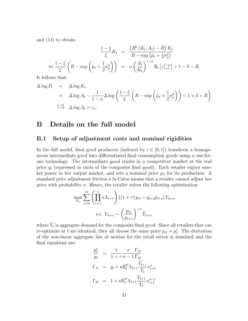
and (14) to obtain:
1− ξξ
Kt =
(Rk (Kt, At)−R
)Kt
R− exp(µt + 1
2σ2µ
)⇔ 1− ξ
ξ
(R− exp
(µt +
1
2σ2µ
))= α
(AtKt
)1−α
Et[ε1−αt+1
]+ 1− δ −R.
It follows that:
∆ logPt = ∆ logKt
= ∆ logAt −1
1− α∆ log
(1− ξξ
(R− exp
(µt +
1
2σ2µ
))− 1 + δ +R
)ξ→1−→ ∆ logAt = εt.
B Details on the full model
B.1 Setup of adjustment costs and nominal rigidities
In the full model, final good producers (indexed by i ∈ [0, 1]) transform a homoge-neous intermediate good into differentiated final consumption goods using a one-for-one technology. The intermediate good trades in a competitive market at the realprice qt (expressed in units of the composite final good). Each retailer enjoys mar-ket power in her output market, and sets a nominal price pit for its production. Astandard price adjustment friction a la Calvo means that a retailer cannot adjust herprice with probability κ. Hence, the retailer solves the following optimization:
maxPit
∞∑s=0
(s∏
τ=1
κΛt+τ
)((1 + τ) pit − qt+spt+s)Yit+s
s.t. Yit+s =
(pitpt+s
)−σYt+s,
where Yt is aggregate demand for the composite final good. Since all retailers that canre-optimize at t are identical, they all choose the same price pit = p∗t . The derivationof the non-linear aggregate law of motion for the retail sector is standard and thefinal equations are:
p∗tpt
=1
1 + τ
σ
σ − 1
Γ1t
Γ2t
Γ1t = qt + κEPt Λt+1Yt+1
Ytπσt+1
Γ2t = 1 + κEPt Λt+1Yt+1
Ytπσ−1t+1
41
I assume that the government sets subsidies such that τ = 1/(σ − 1) so that thesteady-state markup over marginal cost is zero. Inflation πt = pt/pt−1 and the resetprice are linked through the price aggregation equation which can be written as
1 = (1− κ)
(p∗tpt
)1−σ
+ κπσ−1t
and the Tak-Yun distortion term is
∆t = (1− κ)
(Γ1t
Γ2t
)−σ+ κπσt ∆t−1.
This term ∆t ≥ 1 is the wedge due to price distortions between the amount of inter-mediate goods produced and the amount of the final good consumed. The amountof final goods available for consumption and investment is Yt = Yt/∆t. Similarly, onecan define Ct = Ct/∆t as the level of consumption the household could obtain if pricedistortions were zero.
Similarly to retailers, labor agencies transform the homogeneous household laborinput into differentiated labor goods at the nominal price wtpt and sell them to inter-mediate firms at the price wht, which cannot be adjusted with probability κw. Laboragency h solves the following optimization:
maxwht
EPt∞∑s=0
(s∏
τ=1
κwΛt+τ
)((1 + τw)wht − wt+spt+s)Lht+s
s.t. Lht =
(whtwt
)−σwLt
Since all labor agencies that can re-optimize at t are identical, they all choose thesame price wht = w∗t . The first-order conditions are analogous to those for retailers.Again, I assume that the government sets taxes such that τ = 1/(σw − 1) so that thesteady-state markup over marginal cost is zero. Wage inflation πwt and the Tak-Yundistortion ∆wt are defined analogously to final good producers.
Capital good producers operate competitively in input and output markets, produc-ing new capital goods using old final consumption goods. For the latter, they havea CES aggregator just like households. Their maximization program is entirely in-tratemporal:
maxIt
QtIt −(It +
ψ
2
(ItIt−1
− 1
)2)
In particular, they take past investment levels It−1 as given when choosing currentinvestment output. Their first-order condition defines the price for capital goods.
All of the profits made by the firms described above accrue to households. Similarly,all subsidies by the government are financed by lump-sum taxes on households. The
42

market clearing conditions are summarized below. Supply stands on the left-handside, demand on the right-hand side.
Yt =
ˆ 1
0
Yjtdj =
ˆ 1
0
Yitdi
Yt =Yt∆t
= Ct + It +−ψ2
(ItIt−1
− 1
)2
+ Cet
Lt =
ˆ 1
0
Lhtdh
Lt =Lt
∆wt
=
ˆ 1
0
Ljtdj
Kt =
ˆ 1
0
Kjtdj = (1− δ)Kt−1 + It
1 = Sjt, j ∈ [0, 1]
0 = Bgt
B.2 Properties of the rational expectations equilibrium
The rational expectations equilibrium considered here has the following propertiesthat need to be verified. All statements are local in the sense that for each of them,there exists a neighborhood of the non-stochastic steady-state in which the statementholds.
1. All firms choose the same capital-labor ratio Kjt/Ljt .
2. The expected return on capital is higher than the internal return on debt:EtRk
t+1 > Rt.
3. At any time t, the stock market valuation Pjt of a firm j is proportional to itsnet worth after entry and exit Njt with a slope that is strictly greater than one.
4. Borrowers never default on the equilibrium path and borrow at the risk-freerate, and the lender only accepts debt payments up to a certain limit.
5. If the firm defaults and the lender seizes the firm, it always prefers restructuringto liquidation.
6. The firm always exhausts the borrowing limit.
7. All firms can be aggregated. Aggregate debt, capital and net worth are sufficientto describe the intermediate goods sector.
43

I take the following steps to prove the existence of this equilibrium. After settingup the firm value functions, Property 1 just follows from constant returns to scale.I then take Properties 2 and 3 as given and prove 4 to 6. I verify that 3 holds.The aggregation property 7 is then easily verified. I conclude by establishing theparameter restrictions for which 2 holds.
Value functions
An operating firm j enters period t with a predetermined stock of capital and debt.It is convenient to decompose its value function into two stages. The first stage isgiven by:
Υ1 (K,B) = maxN,L,D
γN + (1− γ) (D + Υ2 (N −D))
s.t. N = qY − wL+ (1− δ)QK −RBY = Kα (AL)1−α
D = ζ (N −QK +B)
I suppress the time and firm indices for the sake of notation. After production, thefirm exits with probability γ and pays out all net worth as dividends. The secondstage of the value function consists in choosing debt and capital levels as well as astrategy in the default game:
Υ2
(N)
= maxK′,B′,strategy in default game
βE [Υ1 (K ′, B′) , no default]
+ βE [Υ1 (K ′, B∗) , debt renegotiated]
+ βE [0, lender seizes firm]
s.t. K ′ = N +B′
A firm that only enters in the current period starts directly with an exogenous networth endowment and the value function Υ2.
Characterizing the first stage
The first order conditions for the first stage with respect to L equalizes the wage withthe marginal revenue: w = q (1− α) (K/L)αA1−α. Since there is no firm heterogene-ity apart from capital K and debt B, this already implies Property 1 that all firmschoose the same capital-labor ratio. Hence the internal rate of return on capital iscommon across firms:
Rk = αq
((1− α)
qA
w
) 1−αα
+ (1− δ)Q (43)
44

Taking Property 3 as given for now, Υ2 is a linear function with slope strictly greaterthan one. Then the following holds for the first-stage value function Υ1:
Υ1 (K,B) = N + (1− γ) (D −N + Υ2 (N −D))
= N + (1− γ) (Υ ′2 − 1) ((1− ζ)N + ζ (QK −B))
> N
= RkK −RB (44)
This property will be used repeatedly in the next step of the proof.
Characterizing the second stage
The second stage involves solving for the subgame-perfect equilibrium of the defaultgame between borrower and lender. Pairings are anonymous, so repeated interactionsare ruled out. Also, only the size B and the interest rate R of the loan can becontracted (in equilibrium R = R but this is to be established first). The game isplayed sequentially:
1. The firm (F) proposes a borrowing contract(B, R
).
2. The lender (L) can accept or reject the contract.
• A rejection corresponds to setting the contract(B, R
)= (0, 0).
Payoff for L: 0. Payoff for F: βE[Υ1
(N , 0
)].
3. F acquires capital and can then choose to default or not.
• If F does not default, it has to repay in the next period.
Payoff for L: EQt,t+1RB −B. Payoff for F: βE[Υ1
(K, R
RB)]
.
4. If F defaults, the debt needs to be renegotiated. F makes an offer for a newdebt level B∗.18
5. L can accept or reject the offer.
• If L accepts, the new debt level replaces the old one.
Payoff for L: EΛRB∗ −B. Payoff for F: βE[Υ1
(K, R
RB∗)]
.
6. If L rejects, then she seizes the firm. A fraction 1−ξ of the firm’s capital is lost inthe process. Nature decides randomly whether the firm can be “restructured.”
18That the interest rate on the repayment is fixed is without loss of generality.
45

• If the firm cannot be restructured, or it can but the lender chooses not todo so, then the lender has to liquidate the firm.Payoff for L: EΛξQK −B. Payoff for F: 0.
• If the firm can be restructured and the lender chooses to do so, she retainsa debt claim of present value ξB and sells the residual equity claim in thefirm to another investor.Payoff for L: ξB + βE [Υ1 (ξK, ξB)]−B. Payoff for F: 0.
Backward induction leads to the (unique) subgame-perfect equilibrium of this game.Start with the possibility of restructuring. L prefers this to liquidation if
ξB + βE [Υ1 (ξK, ξB)] ≥ EΛξQK. (45)
This holds true at the steady state because Rk > R (Property 2), Q = 1, β = Λ and
ξB + βE [Υ1 (ξK, ξB)] > ξB + βE[RkξK −RξB
]= βE
[RkξK
]> ξK (46)
Since the inequality is strict, the statement holds in a neighborhood around thesteady-state as well. This establishes Property 5.
Next, L will accept an offer B∗ if it gives her a better expected payoff (assuming thatlenders can diversify among borrowers so that their discount factor is invariant to theoutcome of the game). The probability of restructuring is given by x. The conditionfor accepting B∗ is therefore that
EΛRB∗ ≥ x (ξB + βE [Υ1 (ξK, ξB)]) + (1− x)EΛξQK. (47)
Now turn to the firm F. Among the set of offers B∗ that are accepted by L, the firmwill prefer the lowest one—i.e., that which satisfies (47) with equality. This followsfrom Υ1 being a decreasing function of debt. This lowest offer will be made if it leads
to a higher payoff than expropriation: βE[Υ1
(K, R
RB∗)]≥ 0. Otherwise, F offers
zero and L seizes the firm.
Going one more step backwards, F has to decide whether to declare default or not.It is preferable to do so if the B∗ that L will just accept is strictly smaller than B or
if expropriation is better than repaying, βE[Υ1
(K, R
RB)]≥ 0.
What is then the set of contracts that L accepts in the first place? From the perspec-tive of L, there are two types of contracts: those that will not be defaulted on andthose that will. If F does not default (B∗ ≥ B), L will accept the contract simplyif it pays at least the risk-free rate, R ≥ R. If F does default (B∗ < B), then L
46

accepts if the expected discounted recovery value exceeds the size of the loan—i.e.,EΛRB∗ ≥ B.
Finally, let us consider the contract offer. F can offer a contract on which it will notdefault. In this case, it is optimal to offer just the risk-free rate R = R. Also notethat the payoff from this strategy is strictly positive since
βE [Υ1 (K,B)] > βE[RkK −RB
]= βE
[RkN +
(Rk −R
)B]
> 0. (48)
The payoff is also increasing in the size of the loan B. So conditional on not defaulting,it is optimal for F to take out the maximum loan size B = B∗, and this is preferableto default with expropriation. However, it might also be possible for F to offer acontract that only leads to a default with debt renegotiation. The optimal contractof this type is the solution to the following problem:
maxR,B,B∗
βE
[Υ1
(N +B,
R
RB∗
)]
s.t. EΛRB∗ ≥ B
EΛRB∗ = x(ξB + βE
[Υ1
(ξ(N +B
), ξB
)])+ (1− x)EΛQξ
(N +B
)The first thing to note is that only the product RB∗ appears, so the choice of theinterest rate R is redundant. Further, B = B∗ and R = R solve this problem, and thisamounts to the same as not declaring default. This choice solves the maximizationproblem above if the following condition is satisfied at the steady state:
ξ
R
(1− x+ xR + xΥ ′1
[Rk
R− 1
])< 1 (49)
For the degree of stock price dependence x sufficiently small, this condition is satisfied.This establishes Properties 4 and 6.
Linearity of firm value
Since firms do not default and exhaust the borrowing limit B∗, the second-stage firmvalue can be written as follows:
Υ2
(N)
= βE[Υ1
(N +B,B
)](50)
where B = x(ξB + βE
[Υ1
(ξ(N +B
), ξB
)])+ (1− x)Qξ
(N +B
)(51)
47

We already know that if Υ2 is a linear function, then Υ1 is also linear. The conversealso holds: The constraint above, together with linearity of Υ1 imply that B is linearin N , and thus Υ2 is linear, too.
To establish Property 3, it remains to show that the slope of Υ2 is greater than one.This is easy to see in steady state:
Υ ′2 = βΥ1 (K,B)
N
= βγ(RkK −RB
)+ (1− γ)Υ2
(RkK −RB
)N
= β (γ + (1− γ)Υ ′2)
(RkK
N−RB
N
)= (γ + (1− γ)Υ ′2)
Rk +(Rk −R
)BN
R︸ ︷︷ ︸=:c0>1
=γc0
1− (1− γ) c0
> 1 (52)
Finally, the aggregated law of motion for capital and net worth needs to be established(Property 7). Denoting again by Γt ⊂ [0, 1] the indices of firms that exit and arereplaced in period t, we have
Kt =
ˆ 1
0
Kjtdj =
ˆj /∈Γt
(Njt − ζEjt +Bjt) dj +
ˆj∈Γt
(ω (Nt − ζEt) +Bjt) dj
= (1− γ + γω) (Nt − ζEt) +Bt (53)
Nt =
ˆ 1
0
Njtdj = RktKt−1 −Rt−1Bt−1 (54)
Bt =
ˆ 1
0
Bjtdj = xξ (Bt + Pt) + (1− x) ξEtΛt+1Qt+1Kt (55)
So far, then, all model properties are established except Rk > R.
Return on capital
It can now be shown under which conditions the internal rate of return is indeedgreater than the return on debt. From the steady-state versions of equations (53)and (54), and the definition of earnings E = N −K +B, it follows that
Rk = R +
(1− ζ (1− γ + γω)
(1− ζ) (1− γ + γω)−R
)(1− B
K
). (56)
48

Further, it is straightforward to show that for any combination of parameters, thesteady state of the model has B/K < 1. A necessary and sufficient condition forRk > R is therefore that the first term in parentheses above is strictly positive, orequivalently:
γ >ζ (1− β)
1− ζ (1− β)
1
1− ω . (57)
49