the role of resource predictability in the metapopulation

Purdue UniversityPurdue e-Pubs

Open Access Dissertations Theses and Dissertations

Fall 2013

The Role of Resource Predictability in theMetapopulation Dynamics of InsectsByju Nambidiyattil GovindanPurdue University

Follow this and additional works at: https://docs.lib.purdue.edu/open_access_dissertations

Part of the Ecology and Evolutionary Biology Commons, Entomology Commons, and theNatural Resources and Conservation Commons

This document has been made available through Purdue e-Pubs, a service of the Purdue University Libraries. Please contact [email protected] foradditional information.

Recommended CitationNambidiyattil Govindan, Byju, "The Role of Resource Predictability in the Metapopulation Dynamics of Insects" (2013). Open AccessDissertations. 123.https://docs.lib.purdue.edu/open_access_dissertations/123

https://docs.lib.purdue.edu?utm_source=docs.lib.purdue.edu%2Fopen_access_dissertations%2F123&utm_medium=PDF&utm_campaign=PDFCoverPages

https://docs.lib.purdue.edu/open_access_dissertations?utm_source=docs.lib.purdue.edu%2Fopen_access_dissertations%2F123&utm_medium=PDF&utm_campaign=PDFCoverPages

https://docs.lib.purdue.edu/etd?utm_source=docs.lib.purdue.edu%2Fopen_access_dissertations%2F123&utm_medium=PDF&utm_campaign=PDFCoverPages

https://docs.lib.purdue.edu/open_access_dissertations?utm_source=docs.lib.purdue.edu%2Fopen_access_dissertations%2F123&utm_medium=PDF&utm_campaign=PDFCoverPages

http://network.bepress.com/hgg/discipline/14?utm_source=docs.lib.purdue.edu%2Fopen_access_dissertations%2F123&utm_medium=PDF&utm_campaign=PDFCoverPages



https://docs.lib.purdue.edu/open_access_dissertations/123?utm_source=docs.lib.purdue.edu%2Fopen_access_dissertations%2F123&utm_medium=PDF&utm_campaign=PDFCoverPages

Graduate School ETD Form 9

(Revised 12/07)

PURDUE UNIVERSITY GRADUATE SCHOOL

Thesis/Dissertation Acceptance

This is to certify that the thesis/dissertation prepared

By

Entitled

For the degree of

Is approved by the final examining committee:

Chair

To the best of my knowledge and as understood by the student in the Research Integrity and

Copyright Disclaimer (Graduate School Form 20), this thesis/dissertation adheres to the provisions of

Purdue University’s “Policy on Integrity in Research” and the use of copyrighted material.

Approved by Major Professor(s): ____________________________________

____________________________________

Approved by: Head of the Graduate Program Date

Byju Nambidiyattil Govindan

The Role of Resource Predictability in the Metapopulation Dynamics of Insects

Doctor of Philosophy

Robert K. Swihart Yssa D. DeWoody

Jeffrey D. Holland

Michael R. Saunders

Michael A. Steele

Robert K. Swihart

Robert K. Swihart 11/26/2013

i

THE ROLE OF RESOURCE PREDICTABILITY IN THE METAPOPULATION DYNAMICS OF INSECTS

A Dissertation

Submitted to the Faculty

of

Purdue University

by

Byju Nambidiyattil Govindan

In Partial Fulfillment of the

Requirements for the Degree

of

Doctor of Philosophy

December 2013

Purdue University

West Lafayette, Indiana

ii

To

Rugma and My Parents

iii

ACKNOWLEDGEMENTS

This project would not have been feasible without assistance in the form of

financial or other resources from several sources. Financial support was provided by the

James S. McDonnell Foundation, and by Purdue University in the form of a Graduate

Research Assistantship from the Department of Forestry and Natural Resources, a

Graduate Teaching Assistantship from the Department of Computer and Information

Technology (especially Mrs. Guity Ravai for nearly 3.5 years of support), a Bilsland

Dissertation Fellowship, and a Frederick N. Andrews Environmental Travel Grant. The

U.S. Grain Marketing Research Laboratory in Manhattan, Kansas provided the stock

culture of red flour beetles. Private landowners of Tippecanoe and Warren County,

Indiana, granted access to their properties to collect field data.

Several people helped me from design to completion of this project. I am

extremely grateful to Bryan D. Price, who was instrumental in designing the experimental

landscapes, collecting data on beetles, obtaining permission from private landowners,

designing circle traps, and coordinating field efforts of dozens of technicians to collect

data. G. McGraw, R. Mollenhauer, A. Spikes, A. Moyer, A. Grimm, and several other

field technicians helped to set circle traps and mast traps and collect 4 years of data on

weevils and acorn production. R. S. Anderson, and J. Shukle helped in verifying the

species identity of acorn weevils. N. I. Lichti deserves special mention for aiding me in

iv

study design, GIS analysis and for providing useful feedback on drafts of manuscripts.

Constructive comments by N. A. Urban, K. F. Kellner, J. J. Lusk, H. J. Dalgleish, and

other members of the Swihart lab group helped develop many of the ideas presented in

this dissertation. M. Kéry assisted in the development of single-species occupancy

models, and V. A. A. Jansen provide the base script in Mathematica that was modified to

estimate dispersal parameters for beetles in experimental landscapes. R. P. Poduval

helped format this dissertation. My friends – Vijesh, Tony, Prakashan, Amjath, Dicto,

Meena, Revanna, Joe, Jose, and Vinod, provided constant inspiration and beyond.

Finally, I would like to thank my advisory committee: Zhilan Feng, Jeff Holland,

Yssa DeWoody, and Mike Steele. I would not have gotten this dissertation in its current

form without the guidance from Zhilan (Julie), who always happily crossed State Street

to rescue me whenever I ran out of ideas. Jeff provided me space and resources to

temporarily colonize his lab, helped with identification of weevils, and was always the

first to provide feedback on manuscripts. Without Yssa, it would not have been possible

for me to grasp the metapopulation concept and design the laboratory study to begin this

journey. Mike provided perspective from off campus but remained connected through

emails and my advisor. Special thanks are owed to Mike Saunders, who graciously

accepted the request to join my examination committee. Last but not least, I want to

thank my advisor, Rob Swihart, for being a very dynamic and resourceful mentor, for

connecting me well with all members during our meetings, for supporting me in my dual

degree ambition, and for the constant encouragement and guidance provided through this

timeless journey.

v

TABLE OF CONTENTS

Page

LIST OF TABLES ............................................................................................................. ix LIST OF FIGURES ......................................................................................................... xiii ABSTRACT ............................................................................................................ xvi CHAPTER 1. INTRODUCTION ................................................................................. 1 CHAPTER 2. EXPERIMENTAL BEETLE METAPOPULATIONS RESPOND POSITIVELY TO DYNAMIC LANDSCAPES AND REDUCED CONNECTIVITY .... 8

2.1 Abstract ......................................................................................................8

2.2 Introduction ................................................................................................9

2.3 Methods ....................................................................................................11

2.3.1 Landscapes and Experimental Design .............................................. 11

2.3.1.1 Constructed Landscapes ...................................................................... 12

2.3.1.2 Initial Conditions and Data Collection ................................................ 14

2.3.1.3 Experimental Design ........................................................................... 15

2.4 Statistical Analysis ...................................................................................17

2.4.1 Colonization and Extinction ............................................................. 17

2.4.2 Metapopulation Dynamics ............................................................... 18

2.4.3 Metapopulation Stability .................................................................. 20

2.5 Results ......................................................................................................20

2.5.1 Colonization and Extinction ............................................................. 20


2.5.3 Metapopulation Stability .................................................................. 28

2.6 Discussion ................................................................................................29

vi

Page

CHAPTER 3. INTERMEDIATE DISTURBANCE IN EXPERIMENTAL LANDSCAPES IMPROVES PERSISTENCE OF BEETLE METAPOPULATIONS ... 34

3.1 Abstract ....................................................................................................34

3.2 Introduction ..............................................................................................35

3.3 Methods ....................................................................................................38

3.3.1 Constructed Landscapes ................................................................... 38

3.3.2 Initial Conditions and Data Collection ............................................. 39

3.3.3 Experimental Design ........................................................................ 41

3.3.4 Metapopulation Capacity ................................................................. 42

3.3.5 Metapopulation Persistence .............................................................. 45

3.3.6 Landscape Occupancy ...................................................................... 46

3.3.7 Statistical Modeling .......................................................................... 46

3.4 Results ......................................................................................................47

3.5 Discussion ................................................................................................53

CHAPTER 4. HOST SELECTION AND RESPONSES TO FOREST FRAGMENTATION IN ACORN WEEVILS: INFERENCES FROM DYNAMIC OCCUPANCY MODELS ................................................................................................ 58

4.1 Abstract ....................................................................................................58

4.2 Introduction ..............................................................................................59

4.3 Methods ....................................................................................................63

4.3.1 Field Sampling ................................................................................. 63

4.3.2 Occupancy Modeling ....................................................................... 66

4.3.3 Species Specialization Index ............................................................ 71

4.4 Results ......................................................................................................72

4.4.1 Host Selection .................................................................................. 72

4.4.2 Mast Effects ...................................................................................... 72

4.4.3 Other Environmental Covariates ...................................................... 74


4.4.5 Detection Probability ........................................................................ 75

4.5 Discussion ................................................................................................78

vii

Page

4.5.1 Effects of Fragmentation and Host Preferences on Weevil

Dynamics .......................................................................................... 78

4.5.2 Modeling Dynamics when Detection is Imperfect ........................... 82

4.6 Conclusion ...............................................................................................84

CHAPTER 5. COMMUNITY STRUCTURE OF ACORN WEEVILS IN RELATION TO DYNAMICS OF NUT PRODUCTION: INFERENCES FROM MULTI-SPECIES OCCURRENCE MODELS ................................................................ 86

5.1 Abstract ....................................................................................................86

5.2 Introduction ..............................................................................................87

5.3 Materials and Methods .............................................................................90

5.3.1 Study Area and Study Species ......................................................... 90

5.3.2 Field Sampling ................................................................................. 91

5.3.3 Occupancy Modeling ....................................................................... 91

5.4 Results ....................................................................................................100

5.4.1 Host Selection ................................................................................ 100

5.4.2 Community Level Response .......................................................... 103

5.4.3 Species Level Response ................................................................. 106

5.5 Discussion ..............................................................................................112

CHAPTER 6. CONCLUSION ................................................................................. 118 6.1 Broader Implications and Future Directions ..........................................122

LITERATURE CITED ................................................................................................... 130 APPENDICES

Appendix A WinBUGS Script for Mixed Effect Regression Model in Chapter 2 .....151

Appendix B Distance Matrix Computed from Resource Configuration in 12- Patch

Landscapes .............................................................................................153

Appendix C Density Dependence in Emigration and Estimation of Dispersal Rate .154

Appendix D Distribution of Circle Traps and Curculio Species Abundance on Host

Trees in 2005-2008 ................................................................................160

Appendix E WinBUGS Script for Single-Species Multi-Season Occupancy Model 162

Appendix F WinBUGS Script for Multi-Species Multi-Season Occupancy Model .165

viii

Page

Appendix G Patch Occupancy and Vital Rates for Nine Curculio spp. from

Single-Species Multi-Season Occupancy Models .................................170

Appendix H Effect of Mast on First Year Site Occupancy and Vital Rates for Nine

Curculio spp. from Single-Species Multi-Season Occupancy Models ..172

Appendix I Effect of Mast on Vital Rates for Nine Curculio spp. from Multi-Species

Multi-Season Occupancy Models ..........................................................173

Appendix J Annual Site Occupancy for the Nine Species of Curculio spp.

Multi-Species Multi-Season Occupancy Models ...................................174

VITA…………………………………………………………………………………... 176

ix

LIST OF TABLES

Table .............................................................................................................................. Page

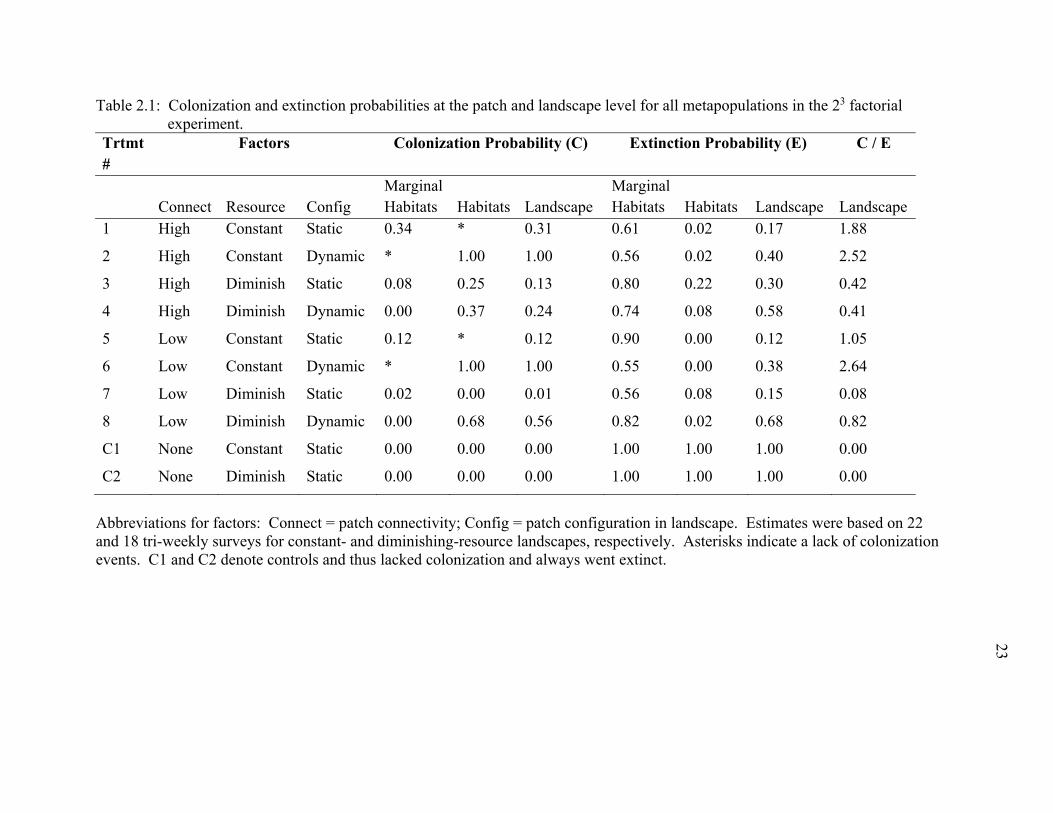
Table 2.1: Colonization and extinction probabilities at the patch and landscape level for all metapopulations in the 23 factorial experiment. ................................................. 23

Table 2.2: Estimates of fixed effect parameters (β) and 95% credible intervals for Poisson mixed effects regressions of adult, larval and pupal counts. ..................... 24

Table 2.3: Mixed effects Poisson regression estimates and 95% credible intervals for landscapes with static patches and control landscapes (with no connectivity). ...... 26

Table 2.4: Mean pupal abundance, strength of negative density dependence (β) on adults and 95% credible intervals. ..................................................................................... 28

Table 3.1: Definitions of frequently used symbols. ......................................................... 37

Table 3.2: Estimate (mean) of abundance of live adults in patches and landscape-level metapopulation attributes for the eight treatments. Standard deviations of estimates are presented in parentheses. For each parameter, treatment means without shared superscripts are different from each other (Tukey sandwich HSD, P < 0.05). ....... 48

Table 3.3: AICc based model-averaged estimates (± adjusted standard error) of predictor variables for landscape-level responses. An asterisk indicates that the 95% credible interval did not contain zero. Refer to Table 3.1 for definitions of symbols used for response and predictor variables. ............................................................................ 50

Table 3.4: Parameter estimate (± SE) and AIC value for models with response variable ‘observed mean abundance of live adult beetles in patches in the landscape’ regressed against predictor variable ‘metapopulation capacity’, estimated by different methods. The AIC value was lowest for the model with λ , as the predictor variable, indicating that the best model incorporated self colonization ability and local population dynamics (i.e., landscape quality). An asterisk indicates that the 95% credible interval did not contain zero. See the text for explanation of predictors. ........................................................................................ 50

x

Table Page

Table 4.1 : Posterior summaries of environmental covariates from dynamic occupancy models fitted to detection data on acorn weevils (Curculio) from 2005 to 2008. Ninety-five percent credible intervals are given in parentheses. For each parameter, ‘Intercept’ refers to baseline probability. ‘Mast’ denotes gross acorn production by white and red oak species. ‘FD100’ is standardized forest density in 100 m radius of host tree, WO indicates host tree species, either a red oak (0) or a white oak (1) and WO*Mast is an interaction term for host tree species and acorn production. An asterisk indicates that the 95% credible interval did not contain zero, whereas a † signifies that a fraction, f, of the posterior distribution was more extreme than zero (see text). All parameters are on the logit scale. .................................................... 73

Table 4.2 : Estimates of average (and standard deviation) nut production per 0.25 m2 by 2 species of trees sampled for acorn weevils. ......................................................... 74

Table 5.1: Circle traps partitioned by host tree species, location in forest stands (core/edge class) and year. Grand total column denotes total number of hosts per tree species for which detection data (along with missing data) on weevils from 2006-08 was used in this study. .............................................................................. 92

Table 5.2: Captures of different Curculio weevil species partitioned by year, host tree species and location (core/edge class) in forest stands. NRO = northern red oak, SBH = shagbark hickory; WO = white oak. .......................................................... 101

Table 5.3: Annual estimates of average (and standard deviation) nut production per 0.25 m2 by 3 species of trees sampled for acorn weevils in west-central Indiana. ....... 102

Table 5.4: Community-level summaries of the hyper-parameters from multi-species multi-season models of acorn weevil occupancy dynamics. A * indicates a hyper-parameter for which the 95% credible interval does not contain zero. ................. 104

Table 5.5: Posterior estimates of mean species richness and 95% credible intervals for Curculio assemblages when host tree species were considered collectively or individually. ........................................................................................................... 106

Table 5.6: Posterior estimates of interannual differences in species richness and 95% credible intervals for Curculio assemblages when host tree species were considered collectively or individually. ................................................................................... 106

Table 5.7: Posterior estimates of mean Jaccard similarity and 95% credible intervals for Curculio assemblages when host tree species were considered collectively or individually. ........................................................................................................... 107

xi

Appendix Table Page Table B 1: Distances (cm) between the patches (dij) in a heterogeneous landscape.

Homogeneous landscapes had a similar configuration, with all the patches being medium sized. Location of a patch in the landscape is represented by coordinates x and y. ..................................................................................................................... 153

Table C 1: Estimate (mean) of species specific attributes for the eight treatment landscapes. Standard deviation of estimate is presented in parenthesis. For each parameter, treatment means with same superscript are not different from each other (Tukey sandwich HSD, P < 0.05). Abundance data from time steps t = 0 to 15 and t = 0 to 23 were used in the estimation of species specific attributes for homogeneous and heterogeneous landscapes, respectively. ................................. 158

Table C 2: AICc based model averaged estimate (± adjusted standard error) of coefficients associated with predictor variables for responses. For each response variable used in regression, estimate for only significant predictors (P ≤ 0.05) is presented. ............................................................................................................... 159

Table D 1: Circle traps partitioned by host tree species, location in forest stands (core/edge class) and year. Grand total column denotes total number of hosts per tree species for which detection data (along with missing data) on weevils from 2005-08 was used in this study. ............................................................................ 160

Table D 2: Captures of different Curculio weevil species partitioned by year, host tree species and location (core/edge class) in forest stands. ........................................ 160

Table G 1: Annual site occupancy for the nine species of Curculio weevils with all host

tree species considered (red oak, white oak and shagbark hickory) and corresponding 95% credible intervals, estimated from single-species occupancy models. Year is indexed in brackets as1-3 and corresponds to 2006-2008, respectively. Survival and colonization rates for each Curculio species correspond to 2006-07 and 2007-08. ....................................................................................... 170

xii

Appendix Table Page Table J 1: Annual site occupancy for the nine species of Curculio weevils on host tree

species and corresponding 95% posterior credible intervals from multi-species occupancy models. Year index 1-3 corresponds to 2006-2008 respectively. ‘All hosts’ model is based on detection data for weevils on 3 host tree species: red oak, white oak and shagbark hickory. ........................................................................... 174

Table J 2: Site-specific vital rates for the nine Curculio species and the 95% credible intervals from multi-species models. .................................................................... 175

xiii

LIST OF FIGURES

Figure ............................................................................................................................. Page

Figure 2.1: Schematic representation of experimental landscapes consisting of two patches of habitat (H, 95% flour and 5% yeast by mass) and two patches of marginal habitat (M, dextrose). Each patch consisted of an inner and outer Petri dish, with resources contained in the inner one. The dark lines projecting from the outer and inner Petri dish denote the paper ramps for dispersing beetles. A small hole on the rim of the outer Petri dish beneath the point where each paper ramps is attached served as an exit hole. Dimensions of the box and patches are not to scale. ........................................................................................................... 12

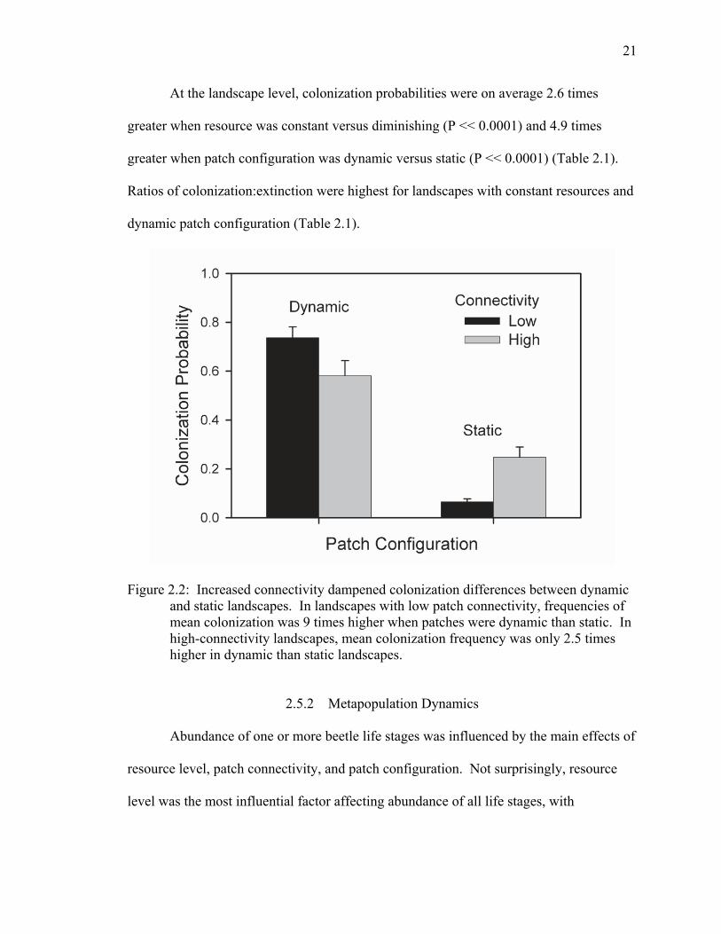
Figure 2.2: Increased connectivity dampened colonization differences between dynamic and static landscapes. In landscapes with low patch connectivity, frequencies of mean colonization was 9 times higher when patches were dynamic than static. In high-connectivity landscapes, mean colonization frequency was only 2.5 times higher in dynamic than static landscapes. ............................................................. 21

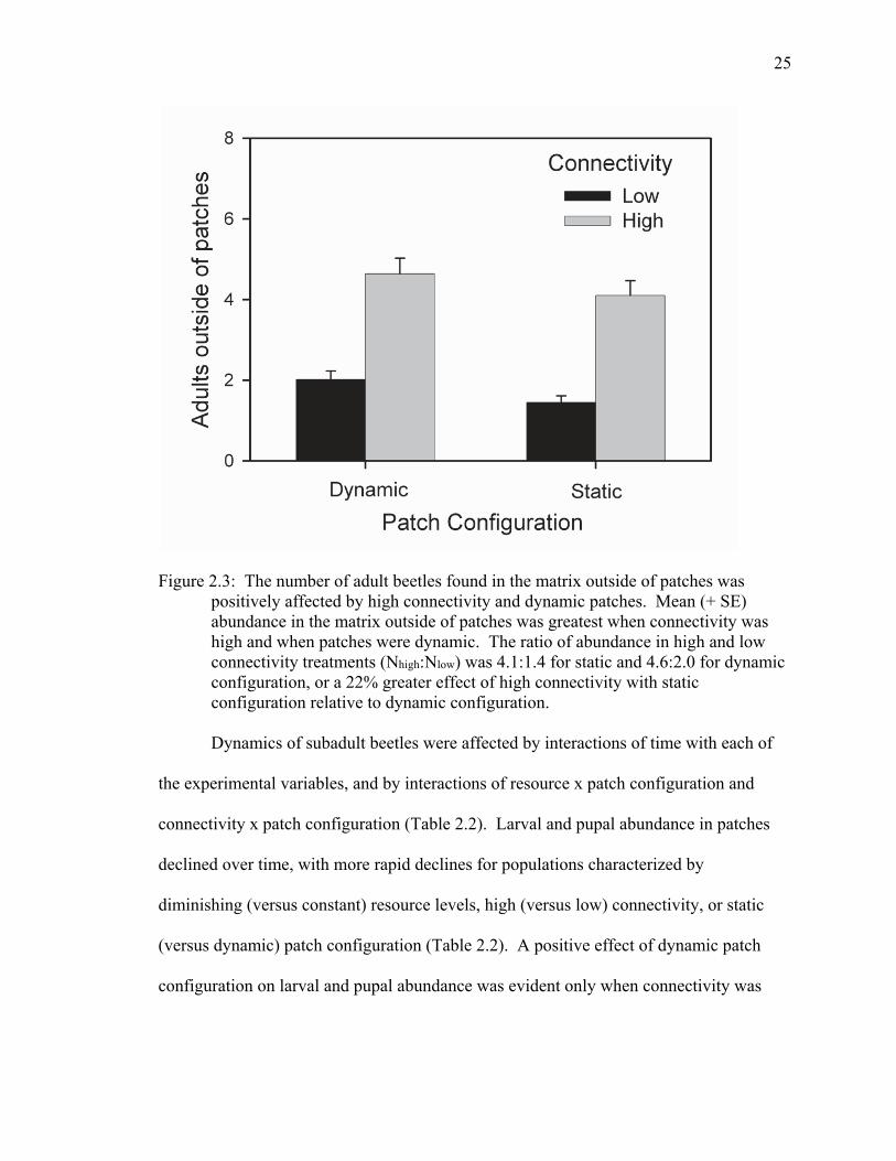
Figure 2.3: The number of adult beetles found in the matrix outside of patches was positively affected by high connectivity and dynamic patches. Mean (+ SE) abundance in the matrix outside of patches was greatest when connectivity was high and when patches were dynamic. The ratio of abundance in high and low connectivity treatments (Nhigh:Nlow) was 4.1:1.4 for static and 4.6:2.0 for dynamic configuration, or a 22% greater effect of high connectivity with static configuration relative to dynamic configuration. .................................................. 25

Figure 2.4: Intermediate levels of connectivity resulted in the greatest abundance of adults in patches. Landscapes with no connectivity resulted in an early increase of adults, followed by relatively rapid declines to extinction. Landscapes with patches that had some connectivity experienced early declines followed by stability over the last half of the study, with greatest abundance for landscapes with low connectivity. Values are means (+ SE) of replicates. ........................... 27

xiv

Figure Page

Figure 3.1: Schematic representation of the 12 patches in the constructed heterogeneous landscape (dimension 59.7 cm x 36.8 cm x 3.8 cm). Low (0.5 g resource), medium (1.5g) and high capacity (3.0g) patches are represented by small, medium and big circles, respectively. The black rectangles on the circles represent the point of exit / entry to the patches. An outer buffer space of 5 cm devoid of patches was included in all landscapes to reduce edge effects. A homogeneous landscape had identical spatial configuration for patches, but had equal carrying capacity for all patches (1.5g). Distance between the patches (in cm) is presented as distance matrix in Appendix B. ........................................................................ 40

Figure 3.2: Interaction effect of resource structure and patch connectivity on the landscape level colonization rate. High connectivity dampened the colonization rate by 41% in landscapes with heterogeneous relative to homogeneous resources................................................................................................................................ 49

Figure 3.3: Mean (± SE) abundance of adult beetles for experimental, 12-patch landscapes with heterogeneous resources, low connectivity, and either no (filled circle), fast (open circle), or slow (triangle) rates of patch turnover. Landscapes with slow turnover exhibited greater metapopulation abundance than landscapes with no turnover, and greater metapopulation persistence than landscapes with fast turnover (Table 3.2). ...................................................................................... 52

Figure 4.1: Observed (circles) and estimated occupancy (squares) with 95% credible intervals (vertical lines) on white and red oak from 2005-2008 for adult Curculio pardalis (top), C. sucatulus (middle), and C. proboscideus (bottom) in landscapes of west-central Indiana. Filled symbols represent red oak and unfilled symbols represent white oak. .............................................................................................. 76

Figure 4.2: Estimated rates of colonization (left panel) and survival (right panel) for local populations of C. pardalis (top), C. sulcatulus (middle), and C. proboscideus (bottom) on white and red oak. Vertical lines are 95% credible intervals. Filled symbols represent red oak and unfilled symbols represent white oak. ................. 77

Figure 4.3: Season and survey-specific estimates of detection probability for C. pardalis (top), C. sulcatulus (middle), and C. proboscideus (bottom) sampled at trees in west-central Indiana from 2005 (solid line), 2006 (dotted line), 2007 (dashed-dotted line), and 2008 (dashed line). ..................................................................... 78

xv

Figure Page

Figure 5.1: Community-level detection probability for the Curculio weevils sampled on all three host tree species, Red oak only and White oak only in west-central Indiana................................................................................................................. 103

Figure 5.2: Season and survey-specific estimates of detection probability for acorn weevils sampled on all three host tree species in west-central Indiana from 2006 (solid line), 2007 (dashed line), and 2008 (dashed dotted line). ......................... 109

Figure 5.3: Estimates of first year site-occupancy (on log scale; filled circles) computed as a function of mast availability for 9 species of Curculio weevils on three species of host trees (red oak, white oak, shagbark hickory) in west-central Indiana, U.S.A. Unfilled circles indicate corresponding estimates of apparent occupancy in first year. Curculio species index on abscissa followed by ‘*’ means 95% credible interval did not contain zero, whereas a † signifies that a fraction, f, of the posterior distribution was more extreme than zero (see text). 110

Figure 5.4: Estimates of survival (filled square) and colonization (filled triangle) probability (on log scale) computed as functions of mast availability for 9 species of Curculio weevils on three species of host trees (red oak, white oak, shagbark hickory) in west-central Indiana, U.S.A. Curculio species index on abscissa followed by ‘*’ means 95% credible interval did not contain zero, whereas a † signifies that a fraction, f, of the posterior distribution was more extreme than zero (see text). ............................................................................................................. 111

Appendix Figure ...................................................................................................................

Figure H 1: Estimates of first year site-occupancy (on log scale) as a function of mast availability derived from single-species models, for nine species of Curculio weevils on three species of host trees (red oak, white oak, shagbark hickory) in west-central Indiana, U.S.A. An asterisk indicates that the 95% credible interval failed to cover zero. All effects of mast production are positive, except for the negative effect of mast on colonization probability for C. sulcatulus. ............... 172

Figure I 1: Estimates of survival (filled square) and colonization (filled triangle) probability (on log scale) as a function of mast availability derived from multi-species occupancy model for 9 species of Curculio weevils on white and red oak species of host trees in west-central Indiana, U.S.A. Curculio species index on abscissa followed by ‘*’ means 95% credible interval did not contain zero, whereas a † signifies that a fraction, f, of the posterior distribution was more extreme than zero (see text). ............................................................................... 173

xvi

ABSTRACT

Govindan, Byju N. Ph.D., Purdue University, December 2013. The Role of Resource Predictability in the Metapopulation Dynamics of Insects. Major Professor: Robert K. Swihart. The metapopulation paradigm has emerged as an important tool to understand the

dynamics of species living in fragmented landscapes. In this dissertation, I investigate

the unpredictable nature of resource availability for species living in human-dominated

heterogeneous and dynamic landscapes in the context of its consequences for long-term

regional persistence of species. In particular, I test theoretical advancements in

metapopulation ecology following a two-pronged approach - via experiments in the lab

and observations in the field - using insects. In chapter 1, I introduce the concept of

metapopulation ecology in the context of its relevance for dynamics of species living in

fragmented landscapes and describe my objectives. In chapter 2, I investigate the main

and interactive effects of resource availability (constant vs. diminishing), patch

connectivity (low vs. high), and dynamics of patch configuration (static vs. dynamic) on

landscape and patch level colonization, extinction and abundance of red flour beetles

(Tribolium castaneum) as well as metapopulation stability. Patch connectivity and

configuration interacted to influence beetle abundance and stability, with intermediate

connectivity and patch dynamics leading to greater persistence. In chapter 3, I test

xvii

predictions of a spatially realistic and temporally dynamic metapopulation model to

assess and compare metapopulation capacity and persistence for red flour beetles in

experimental landscapes differentiated by resource structure (homogeneous vs.

heterogeneous), patch connectivity (high vs. low) and patch dynamics (fast vs. slow), but

with the same background destruction rate. Once again, interactive effects predominated.

Intermediate patch dynamics and connectivity, coupled with density-dependent

emigration promoted persistence in heterogeneous landscapes. In chapter 4, I develop a

characterization of northern red oak (Quercus rubra) and white oak (Q. alba) trees as

resource patches for two generalist and one specialist species of acorn weevil (Curculio)

and employ a Bayesian state space formulation of single-species multi-year dynamic

occupancy modeling to examine the effect of niche breadth, forest structure and

fragmentation on their patch occupancy and vital rates. The specialist species exhibited

greater occupancy than generalists, but its less preferred host tree appeared to serve as a

sink that created greater fluctuations in the specialist metapopulation than in those of the

generalist species. Thus, generalists occurred on a lower proportion of usable trees but

were buffered by access to more suitable patches and greater patch-specific survival. In

Chapter 5, I extend the hierarchical modeling framework to develop multi-species multi-

year dynamic occupancy models to estimate site-specific occupancy, survival and

colonization of nine Curculio species on their primary host tree(s) species, particularly

oaks and shagbark hickory (Carya ovata), and examine the effect of spatio-temporal

variability in resource availability (mast) on the community level coexistence of these

weevils. Local coexistence of weevil species appeared to be promoted by coupling of a

spatial storage effect caused by differential host suitability and a temporal storage effect

xviii

caused by prolonged diapause. Both storage effects were more pronounced for

generalists. In chapter 6, I summarize the key findings of my investigation and briefly

discuss their broader implications and future directions for research.

1

CHAPTER 1. INTRODUCTION

The purpose of this dissertation is to provide empirical tests of theoretical

predictions in the field of metapopulation ecology. In particular, I consider the

unpredictable nature of resource availability for species living in human-dominated

heterogeneous and dynamic landscapes in the context of its consequences for long term

regional persistence of species. My investigations cast light on the utility of recent

theoretical models to address the dynamics of real-world populations occupying

fragmented landscapes, and the factors structuring the community they comprise.

Species living in human-dominated landscapes experience frequent and severe

habitat loss and fragmentation (Hanski 1996, Swihart et al. 2003), which is identified as

the single greatest threat to global biodiversity (Wilcox and Murphy 1985, Debinski and

Holt 2000). Whereas habitat destruction leads to decreased or total loss in carrying

capacity of the habitat patches, fragmentation breaks apart the available habitat into

pieces of isolated patches (Franklin et al. 2002). Both processes alter the spatial structure

of the landscape to isolate the local populations. Dispersal events connect the spatially

isolated populations and facilitate re-colonization of locally extinct patches to prevent

quicker regional extinction of the species (Hanski 1991). Traditional population

dynamics measure changes in number of individuals as a function of only death and birth

in local habitats and ignore dispersal of individuals among local populations. Such an

2

approach is hence insufficient to adequately explain the long-term regional persistence of

species in dynamic landscapes subjected to habitat loss and fragmentation.

As an alternative, the metapopulation paradigm has emerged as an important tool

to understand the dynamics of species living in fragmented landscapes (Hanski 1994). A

metapopulation is a spatially structured population or set of local populations occupying

isolated patches, linked by rare dispersal events (Hanski 1998). Four essential

characteristics of a metapopulation are (Hanski et al. 1995): 1) discrete habitat patches

that support breeding local populations, (2) measurable rates of extinction and (3)

colonization probability for each local population, and (4) asynchrony in local population

dynamics. Dispersal allows re-colonization of individuals from extant neighboring

occupied habitat patches into locally extinct but habitable patches, and asynchrony in

dynamics reduces the chance of simultaneous local extinctions. The metapopulation

concept thus integrates local population dynamics with extinctions and colonization

dynamics and enables estimation of changes in the number of local populations (patch

occupancy) (Hanski 1999b) and factors influencing metapopulation persistence. More

precisely, it serves as an important tool to study the abundance and distribution of species

on larger spatial scales (Levins 1969, Hanski 1989), and thus addresses the pressing

needs for better alternatives to conserve species and protect biodiversity.

Early metapopulation models ignored many real-world features like

environmental and demographic heterogeneity, spatial structure and temporal dynamics

of patches (Bascompte 2001, Harding and McNamara 2002). Advancements in

metapopulation modeling addressed these issues (Gyllenberg and Hanski 1997, Moilanen

and Hanski 1998) and highlighted the significance of spatial (i.e.heterogeneity in patches;

3

Bascompte and Sole1996 ׳, Levin and Durrett 1996, Frank and Wissel 1998, Hill and

Caswell 1999, With and King 1999, Ovaskainen and Hanski 2001) and temporal (patch

dynamics) structure (Keymer et al. 2000, Fahrig 2002, DeWoody et al. 2005) of

landscape on the persistence of species. These investigations concluded that spatial

features like patch size, spatial pattern of patches and connectivity of patches, as well as

temporal features likes changes in spatial configuration of habitable patches and

assumption of local dispersal are essential to understand the dynamics of a population.

For models to be considered generally useful as conservation tools, theoretical

predictions need to be tested and verified with multiple species. Nevertheless progress

has been slow testing predictions in real-world systems (Hodgson et al. 2009).

Challenges include identifying species that exist as metapopulations, difficulties in

disentangling confounding factors in field experiments, an inability to replicate

experiments in natural landscapes and intractability of tracking species in large areas of

natural landscapes. Laboratory experiments employing model organisms offer an

alternate method to test model predictions but have been relatively limited until recently

(Debinski and Holt 2000, Fahrig 2002). I tested theoretical advancements in the

metapopulation ecology following a two-pronged approach - via experiments in the lab

and observations in the field - using insects. Lab experiments were designed with a well-

studied model organism – the red flour beetle, Tribolium castaneum (Desharnais and Liu

1987), and field experiments investigated the dynamics and community structure of a

guild of weevil (Curculio species) seed predators of oak and hickory (Gibson 1964).

Few empirical studies have simultaneously explored effects of multiple factors on

metapopulation dynamics, let alone their interactive effects (Cook and Holt 2006). In

4

chapter 2 of this dissertation, I explore the consequences of spatial (Hill and Caswell

1999, With and King 1999) and temporal (Keymer et al. 2000) dynamics in resource

availability for metapopulation dynamics of red flour beetles. In experimental landscapes

designed with two habitable and two unsuitable habitat patches, I manipulate the resource

availability (constant vs. diminishing), patch connectivity (low vs. high), and dynamics of

patch configuration (static vs. dynamic) to investigate the main and interactive effect of

these factors on colonization, extinction and abundance of beetles as well as

metapopulation stability. I employ quasi-binomial generalized linear models and

Bayesian implementation of generalized linear mixed effect models to test the predictions.

The results indicate that connectivity interacts with patch configuration to influence

metapopulation abundance and stability, both of which were greatest in landscapes with

constant resource, low connectivity and dynamic patches.

Results from chapter 2 clearly highlight the need for additional empirical studies

to explore the impact of patch connectivity, patch turn-over rates, and habitat complexity

on the persistence of metapopulation residing in spatially and temporally varying

landscapes. In Chapter 3, I designed an experimental landscape with higher dimension,

i.e., 12 habitat patches with same or varied carrying capacity. Each of these patches can

exist in three states - uninhabitable, habitable but unoccupied, and habitable and occupied

states, facilitated by patch destruction and recreation over time. I tested the predictions of

a spatially realistic and temporally dynamic metapopulation model developed by Zhilan

Feng and co-workers (DeWoody et al. 2005), to assess and compare metapopulation

capacity and persistence for red flour beetles in experimental landscapes differentiated by

resource structure (homogeneous vs. heterogeneous), patch connectivity (high vs. low)

5

and patch dynamics (fast vs. slow), but with the same background destruction rate. I

estimated the dispersal range of beetles based on the covariance structure in time series

data on adult beetle abundance in patches (Schneeberger and Jansen 2006) and used this

information to develop and estimate an index of metapopulation capacity for different

treatment landscapes. The results demonstrate the importance of incorporating local

dynamics into estimation of metapopulation capacity and highlight the role of

intermediate patch dynamics, intermediate connectivity and the nature of density

dependence of emigration for metapopulation persistence and conservation planning.

In the next two chapters of the dissertation, I extend my investigations into the

field to examine the dynamics and distribution of acorn weevils (Curculio). Chapter 4

develops a characterization of their host trees, which exhibit masting in the fragmented

forests embedded in a human-dominated matrix of agriculture and urbanization, as

resource patches for poorly mobile acorn weevils. These characteristics result in spatio-

temporal dynamics in resource availability for the weevils and hence make it plausible

for them to exist as metapopulations on their host trees. I test the effect of resource

availability, forest structure and fragmentation on the occupancy and vital rates of acorn

weevils with four years of detection – non-detection data for weevils on their host trees,

white oak (Quercus alba) and red oak (Quercus rubra), collected via replicate surveys

during their breeding period, and host level covariates, particularly mast production. In

such dynamic landscapes, generalist weevil species with broad feeding habitat should

exhibit greater occupancy and lower extinction rates on their host trees than specialists

because they will be less susceptible to variation in the availability of resources (Swihart

and Nupp 1998, Swihart et al. 2003), especially in years of heavy acorn production.

6

Additionally, unlike the experiments with beetles in the lab, presence of species in

patches is easily overlooked in the field (Gu and Swihart 2004). To uncouple the true

absence of a species from non-detection, I employed hierarchical modeling that allowed

separate inference on the sampling (detection) process and the underlying ecological

process (occupancy) and reduced the bias in estimation of parameters (MacKenzie et al.

2003, Royle and Kéry 2007, Royle and Dorazio 2008). Specifically, I relied on Bayesian

implementation of single-species multi-year (season) dynamic patch occupancy models

for data on one specialist and two generalist species, to test the predictions and account

for variation in detection probability for species among host trees, survey date and years.

The results indicated greater occupancy rates and lower specialization index for specialist

than generalist species, and demonstrate the need to incorporate vital rates into the

estimation of any specialization index (Julliard et al. 2006) derived solely from

occupancy rates to avoid misleading inferences.

In Chapter 5 of my dissertation, I extend the hierarchical modeling framework to

develop multi-species, multi-year dynamic occupancy models (Dorazio et al. 2006,

Zipkin et al. 2010) to estimate site-specific occupancy, survival and colonization of nine

Curculio species on their primary host tree(s) species, particularly oaks and shagbark

hickory (Carya ovata). I employed this modeling framework with 3 years of detection

non-detection data to test predictions on community-level attributes. I expected greater

occupancy and survival (lower extinction) rate with increases in mast production of host

trees. Further, in mixed hardwood forest stands dominated by red oak, white oak and

shagbark hickory, I expected greater occupancy, survival rate, species richness and

community similarity when all host tree species are in mast phase as opposed to when all

7

or some experience simultaneous mast failure. I derived estimates of species richness

and community similarity from site occupancies, and compared patterns against annual

variation in mast production. The results suggest a spatial storage effect made possible

by differential suitability of hosts as resources for weevil species and a temporal storage

effect induced by prolonged diapause in Curculio, that operate in conjunction to

facilitate their coexistence (Chesson et al. 2004)

8

CHAPTER 2. EXPERIMENTAL BEETLE METAPOPULATIONS RESPOND POSITIVELY TO DYNAMIC LANDSCAPES AND REDUCED CONNECTIVITY

2.1 Abstract

Interactive effects of multiple environmental factors on metapopulation dynamics

have received scant attention. I designed a laboratory study to test hypotheses regarding

interactive effects of factors affecting the metapopulation dynamics of red flour beetle,

Tribolium castaneum. Within a four-patch landscape I modified resource level (constant

and diminishing), patch connectivity (high and low) and patch configuration (static and

dynamic) to conduct a 23 factorial experiment, consisting of 8 metapopulations, each with

3 replicates. For comparison, two control populations consisting of isolated and static

subpopulations were provided with resources at constant or diminishing levels.

Longitudinal data from 22 tri-weekly counts of beetle abundance were analyzed using

Bayesian Poisson generalized linear mixed models to estimate additive and interactive

effects of factors affecting abundance. Constant resource levels, low connectivity and

dynamic patches yielded greater levels of adult beetle abundance. For a given resource

level, frequency of colonization exceeded extinction in landscapes with dynamic patches

when connectivity was low, thereby promoting greater patch occupancy. Negative

density dependence of pupae on adults occurred and was stronger in landscapes with low

connectivity and constant resources; these metapopulations also demonstrated greatest

stability. Metapopulations in control landscapes went extinct quickly, denoting lower

9

persistence than comparable landscapes with low connectivity. When landscape

carrying capacity was constant, habitat destruction coupled with low connectivity

created asynchronous local dynamics and refugia within which cannibalism of pupae

was reduced. Increasing connectivity may be counter-productive and habitat

destruction/recreation may be beneficial to species in some contexts.

2.2 Introduction

Metapopulations are local populations distributed patchily in space and linked by

dispersal (Hanski 1999b). Their viability depends on a variety of habitat and species-

specific features. Models predict that habitat characteristics such as amount (Levins 1969,

Hanski 1994), suitability (Levins 1969, 1970, Moilanen and Hanski 1998), spatial

structure (Frank and Wissel 1998, Hanski and Ovaskainen 2000), and connectivity (Hess

1996, Hanski 1999a) are important determinants of extinction-colonization dynamics and

hence metapopulation persistence. The spatial (Hill and Caswell 1999, With and King

1999) and temporal (Keymer et al. 2000) dynamics in the availability of habitable and

unsuitable habitats also are predicted to have important consequences for metapopulation

dynamics. Unfortunately, few studies have simultaneously explored effects of multiple

factors on metapopulation dynamics. My objective was to test how resource availability,

patch connectivity, and dynamics of patch configuration interact with each other to

influence metapopulations.

Numerous prior studies have examined the role of each of these factors separately.

Level of resource availability (often measured using patch area or quality) has emerged

predictably as an important determinant of metapopulation viability (Bancroft and

10

Turchin 2003). Resource loss can result from either gradual depletion of resources from

a patch or outright destruction of patches. Gradual depletion of resources from a patch,

while reducing carrying capacity, does not alter the connectivity between patches in a

landscape. Rather, gradual depletion can induce higher adult dispersal and mortality and

lower reproduction, while increasing immature mortality and development time (Bancroft

2001). In contrast, rapid destruction of a patch in a landscape reduces the number of

habitats available for occupancy, increases inter-patch distances, decreases connectivity

of resource patches, and can lead to rapid extinction beyond a critical threshold of loss

(Harrison and Bruna 1999, Bancroft 2001).

Reduced connectivity of resource patches has lowered persistence for

metapopulations of fruit flies (Drosophila hydei) (Forney and Gilpin 1989). However,

the relation between connectivity and persistence is not always monotonic, as

intermediate levels of connectivity enhanced persistence for other metapopulations

(Molofsky and Ferdy 2005, Dey and Joshi 2006). Moreover, if local extinction rate

covaries with connectivity or dispersal rate, an anti-rescue effect may lead to reduced

stability and persistence by, e.g., facilitating the spread of contagious disease between

subpopulations, enhancing predation pressure, or synchronizing local population

dynamics (Bascompte and Sole1996 ׳, Hess 1996, Biedermann 2004, Godoy and Costa

2005, Bull et al. 2006, Dey and Joshi 2006).

In dynamic landscapes, i.e., landscapes in which patches are destroyed and re-

created over time, disturbances that render patches unsuitable increase local extinction

and reduce the number of empty habitats available for colonization (DeWoody et al.

2005). Alternatively, patches that are less prone to destruction can serve as refugia and a

11

source of colonists, thereby enhancing the persistence of species living as

metapopulations (Vuilleumier et al. 2007).

I manipulated resource availability, patch connectivity, and dynamics of patch

configuration in experimental metapopulations to investigate their additive and

interactive effects. Specifically, I tested these effects by manipulating the amount of

resources and the level of boundary permeability (Stamps et al. 1987, Stevens et al. 2006)

for red flour beetles (Tribolium castaneum Herbst (Coleoptera: Tenebrionidae)). I tested

the predicted main effects summarized in the preceding paragraphs and examined all

three pairwise interactions on colonization, extinction, and abundance of beetles.

2.3 Methods

2.3.1 Landscapes and Experimental Design

Red flour beetle is a stored grain pest that infests a variety of stored products

worldwide. The stock population (Berlin) of Tribolium castaneum was obtained from the

U.S. Grain Marketing Research Laboratory in Manhattan, Kansas, in 2005. Beetles were

cultured in 95% wheat flour and 5% yeast medium by mass. Beetles were maintained in

an environmental chamber at 33 ± 1˚C and 70 ± 5% relative humidity. The life cycle in T.

castaneum (egg to adult) takes roughly one month, with an average 4 days for egg, 3

weeks for larval and 6 days for pupal development (Park 1948). Adults attain sexual

maturity and start laying eggs in 2-3 days of emergence (Park and Frank 1948). Thus, the

duration of my experiment (23 tri-weekly period) corresponded to 14-16 generations

(Bancroft and Turchin 2003).

12

2.3.1.1 Constructed Landscapes

I designed experimental landscapes with two habitat and two “marginal” habitat

patches, arranged in an alternating sequence (Figure 2.1). Habitat patches consisted of 95%

wheat flour and 5% brewer’s yeast by mass. Preliminary studies demonstrated that this

mixture provided a resource that favored the successful reproduction and survival of the

beetles. “Marginal” habitat patches consisted of powdered cane sugar (dextrose).

Preliminary studies revealed that the dextrose medium prevented successful reproduction

but permitted adult survival (see also Bancroft and Turchin 2003).

Figure 2.1: Schematic representation of experimental landscapes consisting of two patches of habitat (H, 95% flour and 5% yeast by mass) and two patches of marginal habitat (M, dextrose). Each patch consisted of an inner and outer Petri dish, with resources contained in the inner one. The dark lines projecting from the outer and inner Petri dish denote the paper ramps for dispersing beetles. A small hole on the rim of the outer Petri dish beneath the point where each paper ramps is attached served as an exit hole. Dimensions of the box and patches are not to scale.

13

Each constructed landscape consisted (see Figure 2.1) of a 17-cm x 12-cm plastic

box (Pioneer Plastics, Dixon, KY). The floor was painted with white pigmented primer

sealer (William Zinsser and Co., www.zinsser.com) containing fine grain sand to

facilitate beetle traction. To confine insects, the sides of the tray were treated with Fluon

(Northern Products Inc., Woonsocket RI). A patch in a landscape consisted of a small

(35 mm diameter x 10 mm height) Petri dish affixed with glue inside the center of a

larger (60x15 mm) Petri dish. Gluing was done all along the rim of the smaller Petri dish

to seal the base and prevent adults or larvae from crawling under the smaller dish and

thus getting trapped over the course of the experiment. To facilitate beetle movement

between the inner and outer portions of the patch, an inverted-V paper ramp (24 x 4 mm)

was attached to the rim of the inner dish. The lid of the inner small Petri dish was

notched where the inverted-V paper ramp joined the inner Petri dish to allow the exit of

beetles to the outer Petri dish. A circular hole of diameter 2 mm was made in the outer

dish and oriented 180 degrees from the inverted paper ramp of the inner Petri dish to

allow emigration of beetles from a patch into the surrounding landscape. Connectivity,

specifically, patch boundary permeability (Stamps et al. 1987, Moilanen and Hanski 1998,

Stevens et al. 2006), was varied by modifying the height at which these exit holes were

placed. Preliminary trials over a 3-week period demonstrated that patches with holes 2.5

mm above the base of the outer dish exhibited emigration rates 5.8 times greater than

patches with exit holes at a height of 4.0 mm. The entry of beetles back into patches was

facilitated by providing paper ramps (22 x 4 mm) attached to the edge of the outer dish.

The exit holes and entry ramps that facilitated the movement of the beetles into and out of

the surrounding landscape, respectively, were positioned in a small circular area at the

14

center of the landscape, thereby assuring comparable distances to all other patches and

reducing the effects associated with beetles wandering along the edges of the landscape.

Resources were placed inside the smaller dish, which could hold a maximum of 3g of

medium. Keeping the resources concentrated in the interior of the smaller patch

minimized spillover of resources into the matrix. In addition, restricting resources in the

interior dish maintained the exit hole on the outer dish at a constant height.

2.3.1.2 Initial Conditions and Data Collection

All experimental patches received 6 adults and 18 larvae released on 3g of

medium (flour in habitats and dextrose in marginal habitats) inside the small dish of each

patch (total = 24 adults and 72 larvae per landscape). Both adults and larvae were added

as a starter population to mimic more closely established local populations, avoid time

lags, and buffer against crashes associated with density-dependent cannibalism (Bancroft

2001). Initial population sizes were chosen to approximate the maximal carrying

capacity of the landscape, based on preliminary trials. Twenty four adults were used per

landscape, even though estimated carrying capacity was 16, to increase the likelihood that

all life stages were equally distributed in the 4 patches and to increase odds of 1:1 sex

ratios. I observed a sex ratio of 1:1 when sex of 100 random pupae was determined

(unpublished data). For a sample of six individuals, the probability of obtaining all adults

of a single sex in a patch is 0.03, whereas the probability of 2-4 adults of a given sex is

0.78. For larvae, the probability of obtaining 18 individuals of the same sex is 7.6 x 10-6,

and the probability of 7-12 larvae of a given sex is 0.90.

15

For each treatment, observations were made every 3 weeks, a time interval chosen

to correspond with the larval developmental period, allow sufficient time for beetles to

respond to the treatments imposed, and minimize the disturbance associated with

counting. Sifting the resources with #80 mesh sieve retains most of the Tribolium eggs in

the medium (Leelaja et al. 2007). Measurements were made by sifting the resources

using #20 and #80 mesh sieves and counting the number of living larvae, pupae and live

and dead adults in the patches and the surrounding matrix outside the patches. All living

individuals in all life stages were returned to the patch they had occupied during the most

recent count. Live beetles in the matrix also were counted and released back into the

matrix. Experiments were continued for 22 3-week observation periods or until

metapopulation extinction.

2.3.1.3 Experimental Design

I used a factorial design including 3 factors, each at 2 levels, for a total of eight

treatments. Each treatment was replicated three times. The factors were landscape

connectivity, resource level, and patch configuration. Connectivity was manipulated via

high (exit holes at 2.5 mm) and low (holes at 4.0 mm) boundary permeability. Resource

levels of landscapes either remained constant throughout the experiment, i.e., the medium

in each patch was replenished every 3 weeks, or diminished to represent habitat

degradation. For the latter treatment, at the end of every 3-week period, the medium in

habitat and marginal-habitat patches was replaced with fresh medium, but in an amount

reduced by 0.5 g from what had been present in the patch 3 weeks earlier. For instance,

at the end of the first 3 weeks, a habitat patch with 3 g of resource was replenished with

16

2.5 g of fresh resource and similarly, a marginal-habitat patch was replenished with 2.5 g

of dextrose. Reduction of patch resources by 0.5 g every 3 weeks was continued until the

total resource available in a patch was reduced to 0.5 g, at which point a final reduction to

0.2 g was made. Below this resource level cannibalism is quite high (Campbell and

Runnion 2003). Patch configuration was manipulated either by maintaining a fixed

identity of habitat (flour) and marginal-habitat (dextrose) patches for the duration of the

experiment (static), or destroying all habitats and restoring all marginal habitats to habitat

status at tri-weekly intervals (dynamic). For dynamic landscape treatments, the entire

contents of both habitat patches were removed, and all stages of beetles were sieved and

counted. Next, habitat patches were “destroyed”, i.e., converted to marginal-habitat

patches containing dextrose medium. Similarly, marginal-habitat dextrose patches were

restored to habitat patches containing flour medium. Beetles then were returned to the

patch from which they had been counted and whose state had changed (e.g., from habitat

to marginal-habitat). This pattern of habitat destruction and restoration mimics rotational

cropping systems of many agro-ecosystems and incorporated temporal dynamics in

configuration of patches while maintaining a constant carrying capacity for landscape

from a resource perspective.

In addition to the 23 factorial experiments, I included as references two controls

with no landscape connectivity, i.e., no dispersal of beetles from static patches. In one

control, carrying capacity remained constant, whereas in the other carrying capacity

diminished over time as described above. Only static patch configurations were used in

control landscapes, because extinction would be inevitable in landscapes with dynamic

17

patch configuration (i.e., destruction of habitable patches) and no dispersal. Each control

was replicated three times.

2.4 Statistical Analysis

2.4.1 Colonization and Extinction

Probabilities of colonization and extinction for each patch state (habitat or

marginal habitat) were calculated as the proportion of those colonization and extinction

events occurring from time t-1 to time t during 22 tri-weekly surveys (except as noted

below) divided by the total number of patches in a particular state and available for

colonization (i.e., unoccupied) or extinction (occupied) respectively at time t-1. For

analyses involving comparison across landscapes with diminishing resources or controls,

only data from the first 18 tri-weekly surveys were used, because metapopulations in all

three replicate landscapes suffered extinction beyond this time.

Patch extinction was defined as absence of adult beetles at time t after being

occupied by adults at time t-1. Conversely, patch colonization was defined as the

presence of at least one adult in a patch following extinction. Data on colonization and

extinction frequencies in both patch states of each replicate landscape were used to derive

mean colonization and extinction probabilities at the landscape level for each treatment.

Because count data from the experiment were overdispersed, a quasi-binomial

generalized linear model was fitted (R Core Development Team 2009) to the proportion

of successful colonization and extinction events of each landscape. Predicted coefficients

on a logit scale were back transformed to proportions for comparison. For all analyses,

independent variables included level of resource (constant = 1, diminishing = 0),

18

connectivity between patches (high = 1, low = 0) and patch configuration (static = 1,

dynamic = 0). Model selection was conducted using the quasi Akaike Information

Criterion (QAIC) (Burnham and Anderson 2002: 164) to account for overdispersion.

2.4.2 Metapopulation Dynamics

I applied a generalized linear mixed effects Poisson model (GLMM) to determine

how resource level, patch connectivity and patch configuration affected metapopulation

attributes. The GLMM was implemented within a Bayesian framework (Kéry and

Schaub 2011). Specifically, the response trajectory of each landscape was modeled as a

mixture of the population responses shared by all landscapes (fixed effects) and effects

unique to each individual landscape (random effects), enabling me to account for over-

dispersion.

Response variables in the GLMMs included total live adults, live adults inside

patches, adults outside patches, larvae inside patches, and pupae inside patches. I fitted a

repeated measures model with all main and two-way fixed effects and two random effects

using the model:

~

log ∗ ∗ ∗ ∗ ∗

∗ ∗ ∗ ∗ ∗

∗ ∗ ∗ ∗ ∗ ∗

In the model, Cij is the count observed in landscape j (j = 1 to 24) at time step i (i = 1 to

22). The intercept µ represents the grand mean effect, and βs are the coefficients

19

associated with fixed effects. The parameters αj and i account for random variation in

beetle count data due to landscape and time effects, respectively. Uninformative normal

priors with mean zero were used for µ, β, αj and i. Standard deviations of 100 were

specified for the fixed effects parameters, whereas the hyperparameters α and reflect

the random variation due to landscapes and time, respectively, and were drawn from a

Uniform (0, 1) distribution.

My control landscapes lacked connectivity between patches. To model the effect

of complete isolation on the number of live adults in patches, I modified the GLMM

described above to include three levels of connectivity (none = 0, low = 1, high = 2) and

to exclude main and interaction effects associated with patch configuration. I also fitted a

Poisson GLMM to assess the nature of density dependence on pupae and larvae at time t

in patches of control and treatment populations. For this analysis, time and number of

live adult beetles in patches at time t-1 were treated as fixed factors, along with random

landscape and time effects.

The GLMMs were fitted by calling WinBUGS 1.4 (Lunn et al. 2000) directly

from free software package R version 2.9.2 (R Core Development Team 2009) using the

R add-on library R2WinBUGS (R Core Development Team 2009). For each fitted model,

three parallel chains were run, each with 40000 iterations and a thinning rate of 35,

discarding the first 5000 iterations as burn-in. Gelman-Rubin R-hat values (<=1.1) were

used to assess convergence of chains (Brooks and Gelman 1998). My WinBUGS script

is provided as a supplement (Appendix A).

20

2.4.3 Metapopulation Stability

I estimated stability of metapopulations by measuring the mean amplitude of

fluctuations in population size over time. Specifically, I computed a fluctuation index

(Dey and Joshi 2006) representing the mean change in population size from t to t+1,

scaled by average population size over the duration of the study. I estimated fluctuation

indices for all metapopulations and each of the associated subpopulations and performed

an ANOVA on the fluctuation indices to investigate the main and interaction effects of

resource level, connectivity and patch configuration on metapopulation stability. I also

performed an ANOVA on the fluctuation indices estimated for subpopulations in habitat

and marginal habitat with the same set of predictor variables.

2.5 Results

2.5.1 Colonization and Extinction

For colonization frequency, the QAIC-best model included a significant (P =

0.0003) interaction effect of patch connectivity and configuration. Increased connectivity

dampened the positive effect of a dynamic patch configuration on colonization (Figure

2.2). Specifically, colonization frequency (and probability) in landscapes with low patch

connectivity was nearly 10 times greater when patches had dynamic versus static

configuration. In contrast, colonization frequency (probability) in landscapes with high

patch connectivity was only 2.5 times higher when patches were dynamic versus static.

The frequency of patch extinctions was 1.65 times greater for landscapes with

diminishing resources (P = 0.01) and nearly three times greater in landscapes with

dynamic patches (P << 0.001). No interactive effects on patch extinction were observed.

21

At the landscape level, colonization probabilities were on average 2.6 times

greater when resource was constant versus diminishing (P << 0.0001) and 4.9 times

greater when patch configuration was dynamic versus static (P << 0.0001) (Table 2.1).

Ratios of colonization:extinction were highest for landscapes with constant resources and

dynamic patch configuration (Table 2.1).

Figure 2.2: Increased connectivity dampened colonization differences between dynamic and static landscapes. In landscapes with low patch connectivity, frequencies of mean colonization was 9 times higher when patches were dynamic than static. In high-connectivity landscapes, mean colonization frequency was only 2.5 times higher in dynamic than static landscapes.


Abundance of one or more beetle life stages was influenced by the main effects of

resource level, patch connectivity, and patch configuration. Not surprisingly, resource

level was the most influential factor affecting abundance of all life stages, with

22

standardized coefficients that were 1.7-33.8 times larger than the next most influential

main effect (Table 2.2, 2.3). Abundance of each of the beetle life stages also was

affected substantially by pairwise interactions of two or more main effects. The

magnitude of standardized coefficients for significant pairwise interactions of resource

level, patch connectivity, and patch configuration averaged 16% of the corresponding

coefficient for resource level (Table 2.2).

Dynamics of adult beetles were affected by interactions of time with each of the

experimental variables, and by interactions of resource x connectivity and resource x

patch configuration (Table 2.2). Adult abundance in landscapes declined over time, with

more rapid declines for populations characterized by diminishing (versus constant)

resource levels, high (versus low) connectivity, or static (versus dynamic) patch

configuration. Total adult abundance averaged 2.8 times higher in landscapes with

constant resources, and this effect was slightly lower (8%) in landscapes with low

connectivity. Effects of patch configuration were evident only in landscapes with

constant resources and produced an average of 22% more adults when patch

configuration was dynamic. Abundance of beetles outside of patches was time-

dependent, exhibiting greater abundance over time in landscapes with constant resources

compared to those with diminishing resources. The effect of high connectivity on adults

occurring in the matrix was 22% greater for landscapes with static patch configuration

relative to dynamic configuration (Table 2.2, Figure 2.3).

23

23

Table 2.1: Colonization and extinction probabilities at the patch and landscape level for all metapopulations in the 23 factorial experiment.

Trtmt #

Factors Colonization Probability (C) Extinction Probability (E) C / E

Connect Resource Config Marginal Habitats Habitats Landscape

Marginal Habitats Habitats Landscape Landscape

1 High Constant Static 0.34 * 0.31 0.61 0.02 0.17 1.88

2 High Constant Dynamic * 1.00 1.00 0.56 0.02 0.40 2.52

3 High Diminish Static 0.08 0.25 0.13 0.80 0.22 0.30 0.42

4 High Diminish Dynamic 0.00 0.37 0.24 0.74 0.08 0.58 0.41

5 Low Constant Static 0.12 * 0.12 0.90 0.00 0.12 1.05

6 Low Constant Dynamic * 1.00 1.00 0.55 0.00 0.38 2.64

7 Low Diminish Static 0.02 0.00 0.01 0.56 0.08 0.15 0.08

8 Low Diminish Dynamic 0.00 0.68 0.56 0.82 0.02 0.68 0.82

C1 None Constant Static 0.00 0.00 0.00 1.00 1.00 1.00 0.00

C2 None Diminish Static 0.00 0.00 0.00 1.00 1.00 1.00 0.00

Abbreviations for factors: Connect = patch connectivity; Config = patch configuration in landscape. Estimates were based on 22 and 18 tri-weekly surveys for constant- and diminishing-resource landscapes, respectively. Asterisks indicate a lack of colonization events. C1 and C2 denote controls and thus lacked colonization and always went extinct.

24

24

Table 2.2: Estimates of fixed effect parameters (β) and 95% credible intervals for Poisson mixed effects regressions of adult, larval and pupal counts.

Fixed Effect Parameters

TLA TAO Larvae Pupae

Intercept 2.79 (2.6 – 2.97)* 1.75 (1.28 – 2.20)* 3.85 (3.63 – 4.06)* 0.66 (0.05 – 1.24) *

Time -0.28 (-0.34 – -0.21)* 0.08 (-0.26 – 0.42) -0.06 (-0.15 – 0.03) 0.41 (0.04 – 0.78) *

Resource 1.70 (1.45 – 1.95)* 2.41 (1.94 – 2.91)* 2.03 (1.76 – 2.29)* 2.59 (1.86 – 3.34) *

Connect -0.02 (-0.27 – 0.22) 1.39 (0.94 – 1.89)* 0.04 (-0.21 – 0.29) 0.22 (-0.40 – 0.83)

Config -0.14 (-0.37 – 0.09)a -0.10 (-0.54 –0.36) 0.01 (-0.24 – 0.28) 0.05 (-0.59 – 0.68)

Resource x Connect 0.17 (-0.10 – 0.44)b -0.04 (-0.61 – 0.54) 0.14 (-0.18 – 0.43) 0.18 (-0.62 – 0.98)

Resource x Config -0.21 (-0.49 – 0.06)c 0.04 (-0.52 – 0.61) -0.20 (-0.50 – 0.10)e -0.27 (-1.10 – 0.52)

Connect x Config 0.14 (-0.15 – 0.41) 0.59 (0.06 – 1.16)* 0.19 (-0.09 – 0.49)f 0.73 (0.03 – 1.54)*

Time x Resource 1.11 (1.03 – 1.18)* 1.64 (1.43 – 1.87)* 1.34 (1.29 – 1.40)* 1.40 (1.07 – 1.75)*

Time x Connect -0.12 (-0.17 – -0.06)* 0.01 (-0.13 – 0.14) 0.01 (-0.03 – 0.04)g 0.21 (0.05 – 0.37)*

Time x Config -0.05 (-0.11 – 0)d -0.02 (-0.13 – 0.10) 0.08 (0.05 – 0.12)* 0.18 (0.02 – 0.35)*

Data on response variables were collected over 23 3–week periods. Response variable ‘TLA’ stands for total live adults in landscape, and ‘TAO’ for total adults outside patches in landscape. An asterisk indicates that the 95% credible interval did not contain zero. Lower-case superscripts are provided for interaction effects with credible intervals containing zero but for which only a small fraction, f, of the posterior distribution was more extreme than zero. af = 0.11; bf = 0.10; cf = 0.06; df = 0.02; ef = 0.08; ff = 0.11; gf = 0.07.

25

Figure 2.3: The number of adult beetles found in the matrix outside of patches was positively affected by high connectivity and dynamic patches. Mean (+ SE) abundance in the matrix outside of patches was greatest when connectivity was high and when patches were dynamic. The ratio of abundance in high and low connectivity treatments (Nhigh:Nlow) was 4.1:1.4 for static and 4.6:2.0 for dynamic configuration, or a 22% greater effect of high connectivity with static configuration relative to dynamic configuration.

Dynamics of subadult beetles were affected by interactions of time with each of

the experimental variables, and by interactions of resource x patch configuration and

connectivity x patch configuration (Table 2.2). Larval and pupal abundance in patches

declined over time, with more rapid declines for populations characterized by

diminishing (versus constant) resource levels, high (versus low) connectivity, or static

(versus dynamic) patch configuration (Table 2.2). A positive effect of dynamic patch

configuration on larval and pupal abundance was evident only when connectivity was

26

low (Table 2.2), and resulted in 17% more larvae and 86% more pupae than in landscapes

with static configuration. Larval abundance was positively affected by a dynamic

configuration of patches (10% increase relative to static configuration), but only when

resources were constant (Table 2.2).

For landscapes with static patch configuration, including control landscapes,

significant interactions of time x resource and time x connectivity were evident (Table

2.3). The average number of live adults in patches declined over time, and declines were

more rapid for metapopulations with diminishing resource patches. Landscapes with

Table 2.3: Mixed effects Poisson regression estimates and 95% credible intervals for

landscapes with static patches and control landscapes (with no connectivity). Dependent Variable Parameter Β 95% CI

Lower Upper

Live adults in patches Intercept* 2.57 2.39 2.75

Time* -0.24 -0.32 -0.16

Connecta 0.12 -0.09 0.32

Resource* 1.26 1.00 1.52

Time x Resource* 0.91 0.81 1.01

Time x Connect* 0.32 0.26 0.37

Connect x Resource 0.02 -0.28 0.31

For interpretation of *, see footnote for Table 2.2. aThe fraction of the posterior distribution more extreme than zero, f = 0.13.

connected patches tended to have more adult beetles in patches relative to landscapes

with no connectivity (Table 2.3). The interaction effect between time and connectivity

indicated a temporary increase in the number of adults in populations with unconnected

patches, followed by dramatic declines to extinction (Table 2.3). Populations with

connected patches exhibited neither rapid increases nor crashes and stabilized around

27

carrying capacity (Figure 2.4). Results for larval abundance were similar to those for

adults and are not presented here.

Figure 2.4: Intermediate levels of connectivity resulted in the greatest abundance of adults in patches. Landscapes with no connectivity resulted in an early increase of adults, followed by relatively rapid declines to extinction. Landscapes with patches that had some connectivity experienced early declines followed by stability over the last half of the study, with greatest abundance for landscapes with low connectivity. Values are means (+ SE) of replicates.

Poisson GLMM revealed that pupal abundance at time t declined with increasing

adult abundance at time t-1 for both treatment and control landscapes (Table 2.4).

Negative density dependence of pupae was observed in all landscape treatments with

constant resources, with one exception (Table 2.4). In contrast, negative density

dependence was evident in only two landscape treatments with diminishing resources,

and both of these instances involved static patch configuration (Table 2.4). Negative

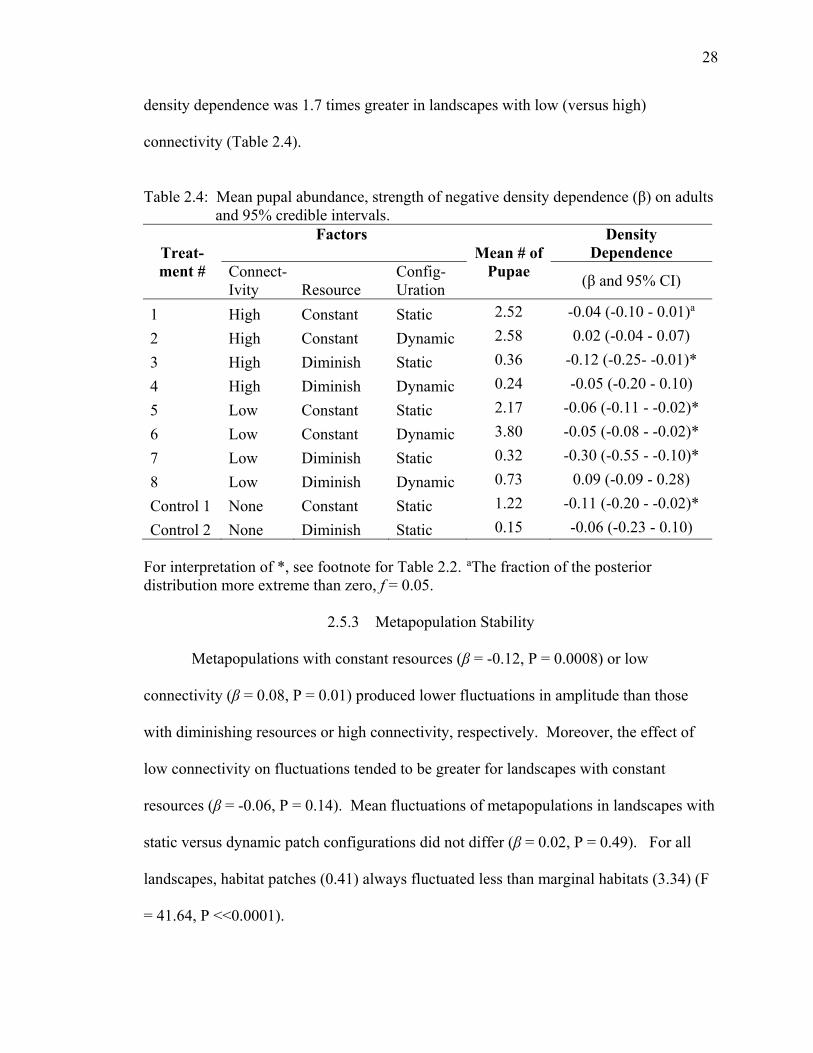
28

density dependence was 1.7 times greater in landscapes with low (versus high)

connectivity (Table 2.4).

Table 2.4: Mean pupal abundance, strength of negative density dependence (β) on adults

and 95% credible intervals.

Treat- ment #

Factors Mean # of

Pupae

Density Dependence

Connect- Ivity Resource

Config- Uration

(β and 95% CI)

1 High Constant Static 2.52 -0.04 (-0.10 - 0.01)a

2 High Constant Dynamic 2.58 0.02 (-0.04 - 0.07)

3 High Diminish Static 0.36 -0.12 (-0.25- -0.01)*

4 High Diminish Dynamic 0.24 -0.05 (-0.20 - 0.10)

5 Low Constant Static 2.17 -0.06 (-0.11 - -0.02)*

6 Low Constant Dynamic 3.80 -0.05 (-0.08 - -0.02)*

7 Low Diminish Static 0.32 -0.30 (-0.55 - -0.10)*

8 Low Diminish Dynamic 0.73 0.09 (-0.09 - 0.28)

Control 1 None Constant Static 1.22 -0.11 (-0.20 - -0.02)*

Control 2 None Diminish Static 0.15 -0.06 (-0.23 - 0.10)

For interpretation of *, see footnote for Table 2.2. aThe fraction of the posterior distribution more extreme than zero, f = 0.05.

2.5.3 Metapopulation Stability

Metapopulations with constant resources (β = -0.12, P = 0.0008) or low

connectivity (β = 0.08, P = 0.01) produced lower fluctuations in amplitude than those

with diminishing resources or high connectivity, respectively. Moreover, the effect of

low connectivity on fluctuations tended to be greater for landscapes with constant

resources (β = -0.06, P = 0.14). Mean fluctuations of metapopulations in landscapes with

static versus dynamic patch configurations did not differ (β = 0.02, P = 0.49). For all

landscapes, habitat patches (0.41) always fluctuated less than marginal habitats (3.34) (F

= 41.64, P <<0.0001).

29

Patterns of fluctuations at the subpopulation level (habitat and marginal habitat)

differed dramatically from those observed for entire metapopulations. Fluctuation in

amplitude was 10 times lower (β = -3.11, P < 0.0001) for habitat patches experiencing

static (0.34) versus dynamic (3.4) configuration, but did not differ for other main effects.

Fluctuations of subpopulations in habitat patches were influenced by the interaction of

resource and configuration (β = -0.18, P < 0.0002) as well as connectivity and

configuration (β = 0.14, P = 0.003). Effects of configuration dominated in both instances,

with greatest fluctuations in habitat patches in dynamic landscapes. When resource

levels were constant, the effect of dynamic patch configuration on fluctuations in habitats

was 1.52 times greater than when resource levels were diminishing. Similarly, when

connectivity of habitat patches was low, the effect of dynamic configuration on

fluctuations was 1.34 times greater than when connectivity was high. Fluctuations in

marginal habitats were lower in landscapes with low patch connectivity (β = -1.61, P =

0.005) and a static configuration of patches (β = -6.06, P < 0.0001), but no interaction

effects were significant.

2.6 Discussion

Beetles in my constructed landscapes met the four criteria for a metapopulation

(Freckleton and Watkinson 2002). Namely, suitable habitat was configured in discrete

patches (Fig. 2.1), local populations experienced measurable rates of extinction (Table

2.1), local population dynamics were not completely synchronized, and dispersing

individuals linked the local populations. Regarding the latter point, dispersal was rare but

sufficient to link local populations, averaging 0.4 (low connectivity) and 1.4 (high

connectivity) individuals per generation.

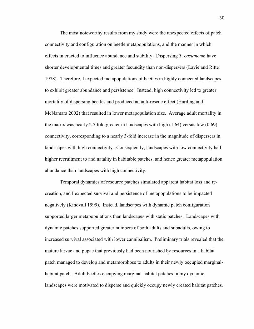
30

The most noteworthy results from my study were the unexpected effects of patch

connectivity and configuration on beetle metapopulations, and the manner in which

effects interacted to influence abundance and stability. Dispersing T. castaneum have

shorter developmental times and greater fecundity than non-dispersers (Lavie and Ritte

1978). Therefore, I expected metapopulations of beetles in highly connected landscapes

to exhibit greater abundance and persistence. Instead, high connectivity led to greater

mortality of dispersing beetles and produced an anti-rescue effect (Harding and

McNamara 2002) that resulted in lower metapopulation size. Average adult mortality in

the matrix was nearly 2.5 fold greater in landscapes with high (1.64) versus low (0.69)

connectivity, corresponding to a nearly 3-fold increase in the magnitude of dispersers in

landscapes with high connectivity. Consequently, landscapes with low connectivity had

higher recruitment to and natality in habitable patches, and hence greater metapopulation

abundance than landscapes with high connectivity.

Temporal dynamics of resource patches simulated apparent habitat loss and re-

creation, and I expected survival and persistence of metapopulations to be impacted

negatively (Kindvall 1999). Instead, landscapes with dynamic patch configuration

supported larger metapopulations than landscapes with static patches. Landscapes with

dynamic patches supported greater numbers of both adults and subadults, owing to

increased survival associated with lower cannibalism. Preliminary trials revealed that the

mature larvae and pupae that previously had been nourished by resources in a habitat

patch managed to develop and metamorphose to adults in their newly occupied marginal-

habitat patch. Adult beetles occupying marginal-habitat patches in my dynamic

landscapes were motivated to disperse and quickly occupy newly created habitat patches.

31

Their dispersal to habitat patches apparently reduced cannibalistic activity in marginal-

habitat patches. At the onset of each tri-weekly period throughout the study, newly

created habitat patches (i.e. transformed marginal habitats) in my dynamic landscapes

had negligibly low adult and egg density, whereas the habitat patches in static landscapes

retained adults and eggs at greater densities. Low initial densities, combined with

gradual recruitment of dispersing adults, likely facilitated enhanced adult fecundity in

newly formed habitat patches of dynamic landscapes (Sonleitner 1961, Sonleitner and

Guthrie 1991). Thus, dynamic landscapes contained patches that changed states between

habitat and marginal habitat, effectively providing refugia for juveniles, pupae and

callows by releasing them from cannibalism (Benoit et al. 1998). Vuilleumier and

coworkers (Vuilleumier et al. 2007) concluded that any patch in a dynamic landscape that

provides refugia can serve as source of colonists for habitats recovering from disturbance,

thereby increasing metapopulation persistence.

Metapopulations with constant resource levels and low connectivity exhibited the

greatest levels of density dependence. Consistent with Desharnais and Liu (1987), these

metapopulations also exhibited the greatest stability. Strong intraspecific competition at

high population densities can reduce population variability and local extinction

probabilities (Taylor and Woiwod 1980, McArdle et al. 1990), as shown experimentally

in my study and in rock pool Daphnia populations (Bengtsson 1989, Bengtsson and

Milbrink 1995).

In my study, reduced patch connectivity increased the difference in colonization

rate between dynamic and static landscapes by 3-30-fold. Connectivity had no effect on

extinction rate, but high connectivity resulted in more adults, and more adult mortality, in

32

the matrix for landscapes with static patch configuration. Thus, the net effect of low

connectivity was increased patch occupancy and abundance for metapopulations in

dynamic landscapes. Despite fluctuations of habitat subpopulations that were 10 times

greater for dynamic landscapes, metapopulations in dynamic landscapes displayed

stability comparable to those in static landscapes. Asynchrony in the dynamics of

subpopulations likely contributed to this effect, which was especially notable when

connectivity was low. Following patch destruction, marginal habitats served as more

effective refugia for mature larvae, pupae and callow when connectivity was low; a

similar effect on recruitment was shown in a coral reef fish (Dascyllus flavicaudus) (Stier

and Osenberg 2010). In contrast, dynamics of subpopulations in static landscapes or with

higher connectivity experienced greater synchrony; habitat patches varied together at

comparable adult densities, and marginal habitat patches were occupied only at low

levels throughout the study. My results agree with those of Dey and Joshi (2006), who

attributed higher stability in less-well-connected fruit fly metapopulations to asynchrony

in neighboring subpopulations. Thus, increasing connectivity may be counter-productive

for some species.

Other investigators have noted potentially deleterious effects of enhanced

connectivity. Hess (1996) predicted an anti-rescue effect with increasing connectivity

among subpopulations owing to increased predation, spread of infectious disease, or

other factors that enhance the local extinction rate relative to recolonization. Molofsky

and Ferdy (2005) found a nonlinear relation between migration rates and persistence time

in metapopulations of the annual plant Cardamine pensylvanica and observed increased

extinction due to increased connectivity when all the subpopulations in a metapopulation

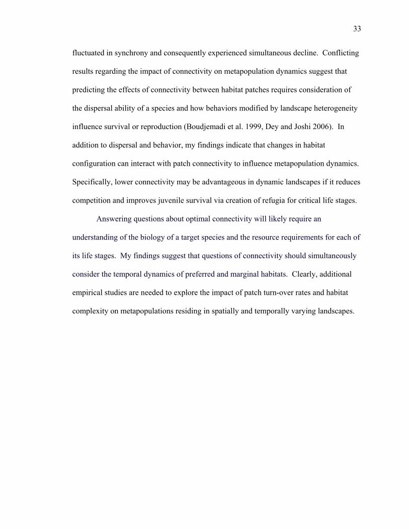
33

fluctuated in synchrony and consequently experienced simultaneous decline. Conflicting

results regarding the impact of connectivity on metapopulation dynamics suggest that

predicting the effects of connectivity between habitat patches requires consideration of

the dispersal ability of a species and how behaviors modified by landscape heterogeneity

influence survival or reproduction (Boudjemadi et al. 1999, Dey and Joshi 2006). In

addition to dispersal and behavior, my findings indicate that changes in habitat

configuration can interact with patch connectivity to influence metapopulation dynamics.

Specifically, lower connectivity may be advantageous in dynamic landscapes if it reduces

competition and improves juvenile survival via creation of refugia for critical life stages.

Answering questions about optimal connectivity will likely require an

understanding of the biology of a target species and the resource requirements for each of

its life stages. My findings suggest that questions of connectivity should simultaneously

consider the temporal dynamics of preferred and marginal habitats. Clearly, additional

empirical studies are needed to explore the impact of patch turn-over rates and habitat

complexity on metapopulations residing in spatially and temporally varying landscapes.

34

CHAPTER 3. INTERMEDIATE DISTURBANCE IN EXPERIMENTAL LANDSCAPES IMPROVES PERSISTENCE OF BEETLE METAPOPULATIONS

3.1 Abstract

Human-dominated landscapes often feature patches that fluctuate in suitability

through space and time, but there is little experimental evidence relating the

consequences of dynamic patches for species persistence. I used a spatially and

temporally dynamic metapopulation model to assess and compare metapopulation

capacity and persistence for red flour beetles (Tribolium castaneum) in experimental

landscapes differentiated by resource structure, patch dynamics (destruction and

restoration) and connectivity. High connectivity increased the colonization rate of beetles,

but this effect was less pronounced in heterogeneous relative to homogeneous landscapes.

Higher connectivity and faster patch dynamics increased extinction rates in landscapes.

Lower connectivity promoted density dependent emigration. Heterogeneous landscapes

containing patches of different carrying capacity enhanced landscape-level occupancy

probability. Highest metapopulation capacity and persistence was observed in landscapes

with heterogeneous patches, low connectivity and slow patch dynamics. Control

landscapes with no patch dynamics exhibited rapid declines in abundance and

approached extinction due to increased adult mortality in the matrix, higher pupal

cannibalism by adults and extremely low rates of exchange between remaining habitable

patches. My results highlight the role of intermediate patch dynamics, intermediate

35

connectivity and the nature of density dependence of emigration for persistence of

species in heterogeneous landscapes. Additionally, my results demonstrate the

importance of incorporating local dynamics into estimation of metapopulation capacity

for conservation planning.

3.2 Introduction

The concept of a metapopulation (Levins 1969), a set of local populations

residing in spatially isolated resource patches connected by dispersal and undergoing

local extinction and recolonization, has emerged as a popular theoretical framework to

understand the dynamics of species in fragmented landscapes (Hanski 1994, Hastings and

Harrison 1994, Hanski and Gilpin 1997). Early models were spatially implicit and

ignored many real-world features of landscapes (Bascompte 2001, Harding and

McNamara 2002). Subsequently, spatially realistic versions of the Levins model (SLRM)

were developed (Moilanen and Hanski 1995, Ovaskainen and Hanski 2001). Temporally

dynamic models (TDKM) of landscape dynamics were then developed by allowing

patches to change in quality over time (Keymer et al. 2000). The characteristic features

of SLRM and TDKM were then merged (DeWoody et al. 2005, Xu et al. 2006) to capture

in an analytically tractable system the spatio-temporal complexities associated with

dynamic, patchy landscapes.

The model of DeWoody et al. (2005), hereafter called the temporally dynamic

spatially realistic metapopulation model (TDSRM), allows a patch at a given spatial

location in the landscape to exist in three possible states: uninhabitable (0), habitable yet

empty (1), and habitable and occupied (2). Each patch i can transition between habitable

and uninhabitable states, determined by the area-dependent rates of patch creation ( )

36

and patch destruction ( ), with and serving as the background creation and

destruction rates, respectively.

⁄

⁄

The long term expected amount of suitable habitat patches in a landscape is given by

⁄ ). The patch transition rate between states is defined by the mean lifetime of a

habitable patch ( 1 ⁄ ). Thus, smaller values of signify higher patch turnover rate.

Altering the patch turnover rates allows patch transitions to occur at substantially

different time scales, even for landscapes with equal long-term habitat suitability ( ).

Metapopulation persistence in the TDSRM thus depends not only on habitat suitability,

but also on the mean patch life time.

The TDSRM defines the rate of local colonization ( ) and extinction ( ) in a

metapopulation in the traditional manner (Hanski 1994, Hanski and Gilpin 1997):

exp

⁄

Local colonization rate is dependent on patch connectivity, which is a function of patch

area ( ), inter-patch distances , and the probability that the neighboring patch (j) is

habitable and occupied ( ). Local extinction rate ( ) is considered inversely

proportional to patch area . For a given landscape, all other parameters that define

either patch colonization or extinction rate are species-specific constants, defined by their

life history characteristics: 1⁄ is the mean dispersal distance of the species, and c and e

are the constants that scale colonization and extinction rates, respectively. DeWoody et

37

al. (2005) thus successfully accounted for spatial heterogeneity (through λ and s) and

temporal structure (through τ) of dynamic patchy landscapes, and the natural history

characteristics of the species through , c and e (See Table 3.1 for definitions of

frequently used symbols).

Table 3.1: Definitions of frequently used symbols. Symbol Definition

Probability of patch i in state j, where j = 0 (uninhabitable), 1(habitable and unoccupied) or 2 (habitable and occupied)

Colonization rate of patch i Extinction rate of patch i Distance between patch i and j

Area of patch i c Colonization rate constant e Extinction rate constant

1 ⁄ Mean dispersal distance ; where = dispersal range of species a Landscape-level growth rate s Long-term expected amount of suitable habitat in landscape ; λ Destruction rate of patch i; destruction rate for landscape

; Creation rate of patch i; creation rate for landscape

Long-term expected life span of habitable patches (1 ⁄ )

Metapopulation capacity following Ovaskainen and Hanski (2000) ; ; , Metapopulation capacity adjusted for self colonization in patches; for

local population dynamics; and for both

Extinction Threshold

Landscape-level effective reproductive number ∗ Expected landscape occupancy

RS; PC; PD Resource structure, Patch connectivity and Patch dynamics respectively

Predictions of metapopulation models that incorporate patch dynamics have been

subjected to few empirical tests (Hodgson et al. 2009), and I am not aware of empirical

applications of the TDSRM. Here, I apply the TDSRM to examine the effects of patch

38

connectedness and resource distribution on metapopulation capacity and persistence for

beetles in experimental landscapes with fast or slow dynamics. I predicted greater

occupancy and persistence: 1) in heterogeneous landscapes consisting of patches varying

in quality relative to homogeneous landscapes with comparable resources distributed

uniformly among patches, because larger patches within heterogeneous landscapes have

larger carrying capacity and can contribute more immigrants to neighboring patches,

thereby increasing their connectivity; 2) for landscapes with higher connectivity among

patches, due to increase in colonization rates; 3) for landscapes with slower rates of patch

(habitat) creation and destruction, due to lower extinction rates. I also examined

interactive effects of landscape heterogeneity, connectivity, and patch dynamics on

occupancy and metapopulation persistence.

3.3 Methods

My experiments were performed with red flour beetles [Tribolium castaneum

Herbst (Coleoptera: Tenebrionidae)]. Information on stock culture, rearing, and life

history is provided elsewhere (Govindan and Swihart 2012). The duration of the study

(23 tri-weekly periods) corresponded to 14-16 generations (1 generation [i.e. egg to adult]

of beetles ~ 30 days).

3.3.1 Constructed Landscapes

I designed experimental landscapes in the laboratory, each with 12 patches that

underwent manipulation throughout the study. Habitable patches consisted of 95% wheat

flour and 5% brewer’s yeast by mass (maximum of 3 g) to provide nourishment to larvae

and adult beetles; uninhabitable patches lacked resources.

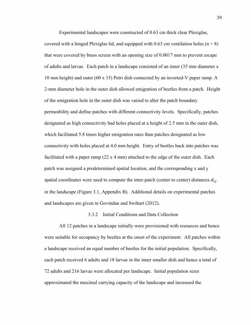
39

Experimental landscapes were constructed of 0.63 cm thick clear Plexiglas,

covered with a hinged Plexiglas lid, and equipped with 0.63 cm ventilation holes (n = 8)

that were covered by brass screen with an opening size of 0.0017 mm to prevent escape

of adults and larvae. Each patch in a landscape consisted of an inner (35 mm diameter x

10 mm height) and outer (60 x 15) Petri dish connected by an inverted-V paper ramp. A

2-mm diameter hole in the outer dish allowed emigration of beetles from a patch. Height

of the emigration hole in the outer dish was varied to alter the patch boundary

permeability and define patches with different connectivity levels. Specifically, patches

designated as high connectivity had holes placed at a height of 2.5 mm in the outer dish,

which facilitated 5.8 times higher emigration rates than patches designated as low

connectivity with holes placed at 4.0 mm height. Entry of beetles back into patches was

facilitated with a paper ramp (22 x 4 mm) attached to the edge of the outer dish. Each

patch was assigned a predetermined spatial location, and the corresponding x and y

spatial coordinates were used to compute the inter-patch (center to center) distances

in the landscape (Figure 3.1, Appendix B). Additional details on experimental patches

and landscapes are given in Govindan and Swihart (2012).

3.3.2 Initial Conditions and Data Collection

All 12 patches in a landscape initially were provisioned with resources and hence

were suitable for occupancy by beetles at the onset of the experiment. All patches within

a landscape received an equal number of beetles for the initial population. Specifically,

each patch received 6 adults and 18 larvae in the inner smaller dish and hence a total of

72 adults and 216 larvae were allocated per landscape. Initial population sizes

approximated the maximal carrying capacity of the landscape and increased the

40

likelihood that all life stages were equally distributed and odds of 1:1 sex ratios in all

patches (Govindan and Swihart 2012). Every 3 weeks I counted the number of living

larvae, pupae and live and dead adults in the patches and the surrounding matrix outside

the patches. Live individuals in all life stages were returned to the patch or location in

the matrix they had occupied during the most recent count. Experiments were continued

for 23 3-week observation periods or until metapopulation extinction.

Figure 3.1: Schematic representation of the 12 patches in the constructed heterogeneous landscape (dimension 59.7 cm x 36.8 cm x 3.8 cm). Low (0.5 g resource), medium (1.5g) and high capacity (3.0g) patches are represented by small, medium and big circles, respectively. The black rectangles on the circles represent the point of exit / entry to the patches. An outer buffer space of 5 cm devoid of patches was included in all landscapes to reduce edge effects. A homogeneous landscape had identical spatial configuration for patches, but had equal carrying capacity for all patches (1.5g). Distance between the patches (in cm) is presented as distance matrix in Appendix B.

41

3.3.3 Experimental Design

To test my predictions based on the TDSRM, I designed a 23 factorial experiment

within constructed landscapes. My design was comprised of three factors, each at 2

levels – patch quality (homogenous or heterogeneous landscape), connectivity (low vs.

high) and dynamics (slow vs. fast). In a homogenous landscape each of the 12 patches

received k = 1.67 g of resource. In a heterogeneous landscape, 4 “large” patches received

3 g, 4 “medium” received 1.5 g, and 4 “small” received 0.5 g of resources (mean value of

k across patches = 1.67 g, see Figure 3.1). Connectivity was manipulated via high (exit

holes at 2.5 mm) and low (holes at 4.0 mm) boundary permeability (Govindan and

Swihart 2012). I manipulated the mean lifetime of patches, , to vary the timescales for

patch destruction and restoration and thus define landscapes with slow or fast patch

dynamics. In landscapes with faster patch dynamics, the habitable patches had a shorter

mean lifespan (τ = 1 week) as compared to the habitable patches in landscapes with slow

patch dynamics (τ = 3 weeks). Thus, ‘fast’ landscapes contained patches that transitioned

more quickly on average between habitat destruction (uninhabitable) and restoration

(habitable). I maintained at 20% the long-term amount of patches in an uninhabitable

state 1 ⁄ in all landscapes over the course of study to facilitate

comparisons across treatments. The state of patches in terms of their suitability for

occupancy was tracked and manipulated on a weekly basis.

In a homogenous landscape, all patches had identical destruction and creation

rates, with mean turnover of 9 and 3 weeks for slow and fast dynamics, respectively. In a

heterogeneous landscape, the three types of patches (small, medium and large) had

different turnover rates reflecting their different capacities. Specifically, low (0.5 g),

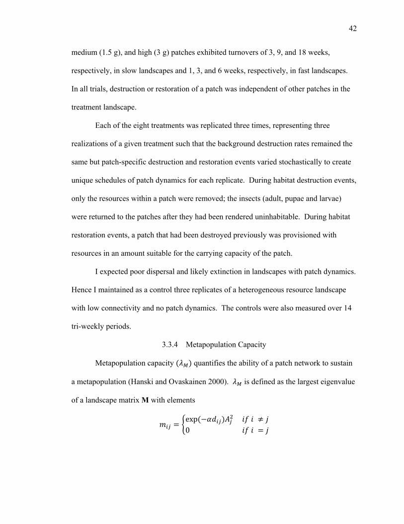
42

medium (1.5 g), and high (3 g) patches exhibited turnovers of 3, 9, and 18 weeks,

respectively, in slow landscapes and 1, 3, and 6 weeks, respectively, in fast landscapes.

In all trials, destruction or restoration of a patch was independent of other patches in the

treatment landscape.

Each of the eight treatments was replicated three times, representing three

realizations of a given treatment such that the background destruction rates remained the

same but patch-specific destruction and restoration events varied stochastically to create

unique schedules of patch dynamics for each replicate. During habitat destruction events,

only the resources within a patch were removed; the insects (adult, pupae and larvae)

were returned to the patches after they had been rendered uninhabitable. During habitat

restoration events, a patch that had been destroyed previously was provisioned with

resources in an amount suitable for the carrying capacity of the patch.

I expected poor dispersal and likely extinction in landscapes with patch dynamics.

Hence I maintained as a control three replicates of a heterogeneous resource landscape

with low connectivity and no patch dynamics. The controls were also measured over 14

tri-weekly periods.

3.3.4 Metapopulation Capacity

Metapopulation capacity quantifies the ability of a patch network to sustain

a metapopulation (Hanski and Ovaskainen 2000). is defined as the largest eigenvalue

of a landscape matrix M with elements

exp 0

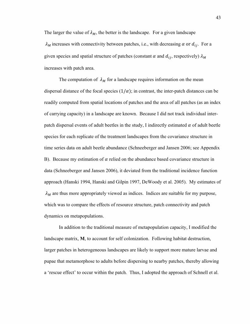
43

The larger the value of , the better is the landscape. For a given landscape

increases with connectivity between patches, i.e., with decreasing or . For a

given species and spatial structure of patches (constant and , respectively)

increases with patch area.

The computation of for a landscape requires information on the mean

dispersal distance of the focal species (1/ ; in contrast, the inter-patch distances can be

readily computed from spatial locations of patches and the area of all patches (as an index

of carrying capacity) in a landscape are known. Because I did not track individual inter-

patch dispersal events of adult beetles in the study, I indirectly estimated of adult beetle

species for each replicate of the treatment landscapes from the covariance structure in

time series data on adult beetle abundance (Schneeberger and Jansen 2006; see Appendix

B). Because my estimation of relied on the abundance based covariance structure in

data (Schneeberger and Jansen 2006), it deviated from the traditional incidence function

approach (Hanski 1994, Hanski and Gilpin 1997, DeWoody et al. 2005). My estimates of

are thus more appropriately viewed as indices. Indices are suitable for my purpose,

which was to compare the effects of resource structure, patch connectivity and patch

dynamics on metapopulations.

In addition to the traditional measure of metapopulation capacity, I modified the

landscape matrix, M, to account for self colonization. Following habitat destruction,

larger patches in heterogeneous landscapes are likely to support more mature larvae and

pupae that metamorphose to adults before dispersing to nearby patches, thereby allowing

a ‘rescue effect’ to occur within the patch. Thus, I adopted the approach of Schnell et al.

44

(2013) and estimated metapopulation capacity with self colonization ( ) by taking the

leading eigenvalue of M with nonzero diagonal elements , .

I also modified M to incorporate local dynamics. ignores local population

dynamics, despite its utility in signifying local habitat quality. I incorporated local

dynamics by using the leading eigenvalue of M with the patch area substituted by

effective carrying capacity (effective patch area). I defined effective carrying capacity

for patches in the landscape as the product of and the patch-specific per capita growth

rate ( ). Because I do not know patch-level growth rates, I have assumed that patch-

level ( ) and landscape-level growth rates (a) are equivalent. Even if this is not the case,

landscape-level growth ratemay be useful as an indicator of the quality of dynamic

landscapes. My logic is consistent with the previous finding that expected life time of a

metapopulation can be increased by increasing the patch capacity by a constant factor

(Drechsler and Wissel 1998). My use of landscape-level growth rate is also analogous to

the density function used by Ackakaya et al. (2004) for estimation of optimal carrying

capacity to predict metapopulation viability in dynamic landscapes. Accordingly,

metapopulation capacity with local dynamics ( ) was computed from the leading

eigenvector of M with elements given by

for :exp 0

Metapopulation capacity with self colonization and local dynamics ( , ) was

computed from the leading eigenvector of M with elements given by

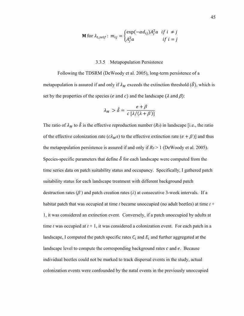
45

for , :exp

3.3.5 Metapopulation Persistence

Following the TDSRM (DeWoody et al. 2005), long-term persistence of a

metapopulation is assured if and only if exceeds the extinction threshold ( , which is

set by the properties of the species ( and and the landscape and :

⁄

The ratio of to is the effective reproduction number (R0) in landscape [i.e., the ratio

of the effective colonization rate ( ) to the effective extinction rate ( )] and thus

the metapopulation persistence is assured if and only if R0 > 1 (DeWoody et al. 2005).

Species-specific parameters that define for each landscape were computed from the

time series data on patch suitability status and occupancy. Specifically, I gathered patch

suitability status for each landscape treatment with different background patch

destruction rates ( ) and patch creation rates (λ) at consecutive 3-week intervals. If a

habitat patch that was occupied at time t became unoccupied (no adult beetles) at time t +

1, it was considered an extinction event. Conversely, if a patch unoccupied by adults at

time t was occupied at t + 1, it was considered a colonization event. For each patch in a

landscape, I computed the patch specific rates and and further aggregated at the

landscape level to compute the corresponding background rates and . Because

individual beetles could not be marked to track dispersal events in the study, actual

colonization events were confounded by the natal events in the previously unoccupied

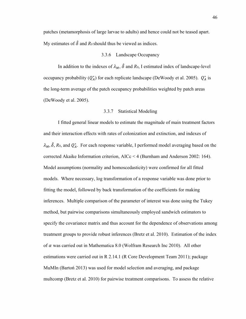
46

patches (metamorphosis of large larvae to adults) and hence could not be teased apart.

My estimates of and R0 should thus be viewed as indices.

3.3.6 Landscape Occupancy

In addition to the indexes of , and R0, I estimated index of landscape-level

occupancy probability ( ∗ ) for each replicate landscape (DeWoody et al. 2005). ∗ is

the long-term average of the patch occupancy probabilities weighted by patch areas

(DeWoody et al. 2005).

3.3.7 Statistical Modeling

I fitted general linear models to estimate the magnitude of main treatment factors

and their interaction effects with rates of colonization and extinction, and indexes of

, , R0, and ∗ . For each response variable, I performed model averaging based on the

corrected Akaike Information criterion, AICc < 4 (Burnham and Anderson 2002: 164).

Model assumptions (normality and homoscedasticity) were confirmed for all fitted

models. Where necessary, log transformation of a response variable was done prior to

fitting the model, followed by back transformation of the coefficients for making

inferences. Multiple comparison of the parameter of interest was done using the Tukey

method, but pairwise comparisons simultaneously employed sandwich estimators to

specify the covariance matrix and thus account for the dependence of observations among

treatment groups to provide robust inferences (Bretz et al. 2010). Estimation of the index

of was carried out in Mathematica 8.0 (Wolfram Research Inc 2010). All other

estimations were carried out in R 2.14.1 (R Core Development Team 2011); package

MuMIn (Bartoń 2013) was used for model selection and averaging, and package

multcomp (Bretz et al. 2010) for pairwise treatment comparisons. To assess the relative

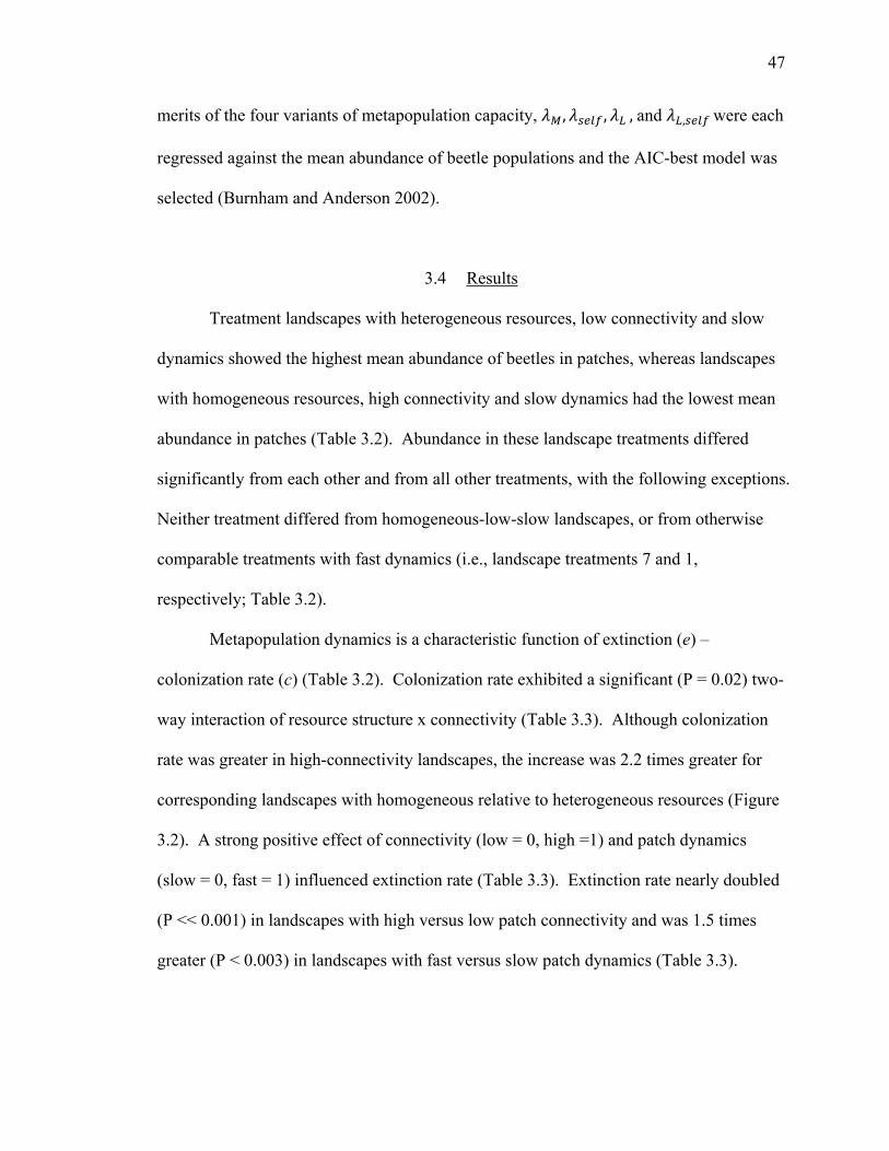
47

merits of the four variants of metapopulation capacity, , , ,and , were each

regressed against the mean abundance of beetle populations and the AIC-best model was

selected (Burnham and Anderson 2002).

3.4 Results

Treatment landscapes with heterogeneous resources, low connectivity and slow

dynamics showed the highest mean abundance of beetles in patches, whereas landscapes

with homogeneous resources, high connectivity and slow dynamics had the lowest mean

abundance in patches (Table 3.2). Abundance in these landscape treatments differed

significantly from each other and from all other treatments, with the following exceptions.

Neither treatment differed from homogeneous-low-slow landscapes, or from otherwise

comparable treatments with fast dynamics (i.e., landscape treatments 7 and 1,

respectively; Table 3.2).

Metapopulation dynamics is a characteristic function of extinction (e) –

colonization rate (c) (Table 3.2). Colonization rate exhibited a significant (P = 0.02) two-

way interaction of resource structure x connectivity (Table 3.3). Although colonization

rate was greater in high-connectivity landscapes, the increase was 2.2 times greater for

corresponding landscapes with homogeneous relative to heterogeneous resources (Figure

3.2). A strong positive effect of connectivity (low = 0, high =1) and patch dynamics

(slow = 0, fast = 1) influenced extinction rate (Table 3.3). Extinction rate nearly doubled

(P << 0.001) in landscapes with high versus low patch connectivity and was 1.5 times

greater (P < 0.003) in landscapes with fast versus slow patch dynamics (Table 3.3).

48

48

Table 3.2: Estimate (mean) of abundance of live adults in patches and landscape-level metapopulation attributes for the eight

treatments. Standard deviations of estimates are presented in parentheses. For each parameter, treatment means without shared superscripts are different from each other (Tukey sandwich HSD, P < 0.05).

Trt #

RS PC PD Abundance

E C , R0 ∗

1 Homogeneous High Fast 3.20bc (0.32)

0.19c (0.03)

0.75d (0.05)

1.99ef (0.13)

69.95b (24.66)

34.84c (10.34)

0.88a

(0.02)

2 Homogeneous High Slow 2.87b (0.16)

0.12b

(0.01) 0.75d (0.05)

0.75 (0.04)

81.23b (24.73)

108.10ab (29.89)

0.89a (0.01)

3 * Homogeneous Low Fast 3.56c (0.24)

0.10ab (0.02)

0.52c (0.04)

2.65g (0.27)

70.76b (16.13)

26.58bc (3.34)

0.89ab (0.03)

4 Homogeneous Low Slow 3.69abc (0.49)

0.07a (0.03)

0.37a (0.08)

1.39bc (0.34)

83.83b (6.86)

61.91b (10.98)

0.86a

(0.04)

5 ** Heterogeneous High Fast 3.61c (0.21)

0.18c (0.01)

0.69bd (0.01)

2.13de (0.02)

72.03b (17.47)

33.91c (8.56)

0.91ab

(0.01)

6 Heterogeneous High Slow 3.49c (0.25)

0.14bc (0.02)

0.66bd (0.04)

0.88a (0.04)

73.06b (1.56)

82.71b (3.18)

0.91ab

(0.02)

7 ** Heterogeneous Low Fast 4.27a (0.20)

0.10ab (0.00)

0.50abc (0.15)

2.86bcdfg (0.85)

111.04b (39.93)

42.77bc ( 26.65)

0.91ab

(0.04)

8 ** Heterogeneous Low Slow 4.53a (0.33)

0.08a (0.02)

0.49ac (0.09)

1.06a (0.15)

211.72a (18.31)

202.70a (46.17)

0.94b

(0.01)

* or ** Mean± SD is based on two replicates [* One replicate for this treatment (#3) suffered fungal infestation, and ** 95% credible interval for the dispersal rate estimated for one replicate each for treatments #5, #7 and #8 contained zero; data from corresponding replicates were not included in analysis]. Refer to Table 3.1 for definitions of symbols used for predictor and response variables. Trt # denotes the treatments from 1–8.

49

Figure 3.2: Interaction effect of resource structure and patch connectivity on the

landscape level colonization rate. High connectivity dampened the colonization rate by 41% in landscapes with heterogeneous relative to homogeneous resources.

For persistence of species in dynamic landscapes, however, the metapopulation

capacity defined by must exceed the extinction threshold defined by factors governing

metapopulation dynamics (c and e) and patch dynamics ( and λ). Estimates of

metapopulation capacity for treatment landscapes varied substantially among the four

different metrics I considered. The slope of observed mean abundances of beetles

against different variants of metapopulation capacity was significant only when the

predictor variable was , , and the equivalent model had the lowest AIC (Table 3.4),

50

50

Table 3.3: AICc based model-averaged estimates (± adjusted standard error) of predictor variables for landscape-level responses. An asterisk indicates that the 95% credible interval did not contain zero. Refer to Table 3.1 for definitions of symbols used for response and predictor variables.

Response Variable

Intercept Predictors (Coefficient ± adjusted SE)1

RS PC PD RS X PC RS X PC*PD c 0.47 ± 0.04 * 0.07 ± 0.05 0.28 ± 0.06* 0.06 ± 0.04 -0.14 ± 0.06* e 0.11 ± 0.01* 0.01 ± 0.01 0.08 ± 0.01* 0.04 ± 0.01*

, 62.55 ± 18.57* 73.78 ± 26.85* 7.40 ± 22.37 30.94 ± 23.14 -79.65 ± 33.33* 97.86 ± 37.40* R0 23.49 ± 18.43 149.06 ± 42.20* ∗ 0.88 ± 0.01* 0.04 ± 0.01* 0.001 ± 0.01 -0.002 ± 0.01

1Two-way interactions RS x PD and PC x PD were not significant for any response variable.

Table 3.4: Parameter estimate (± SE) and AIC value for models with response variable ‘observed mean abundance of live adult

beetles in patches in the landscape’ regressed against predictor variable ‘metapopulation capacity’, estimated by different methods. The AIC value was lowest for the model with , as the predictor variable, indicating that the best model incorporated self colonization ability and local population dynamics (i.e., landscape quality). An asterisk indicates that the 95% credible interval did not contain zero. See the text for explanation of predictors.

Predictor Intercept Coefficient AIC

, 2.91 ± 0.24 * 0.007 ± 0.002 * 29.35 3.26 ± 0.23 * 0.005 ± 0.003 35.25

3.04 ± 0.36 * 0.003 ± 0.002 35.67 3.59 ± 0.28 * 0.00 ± 0.002 38.19

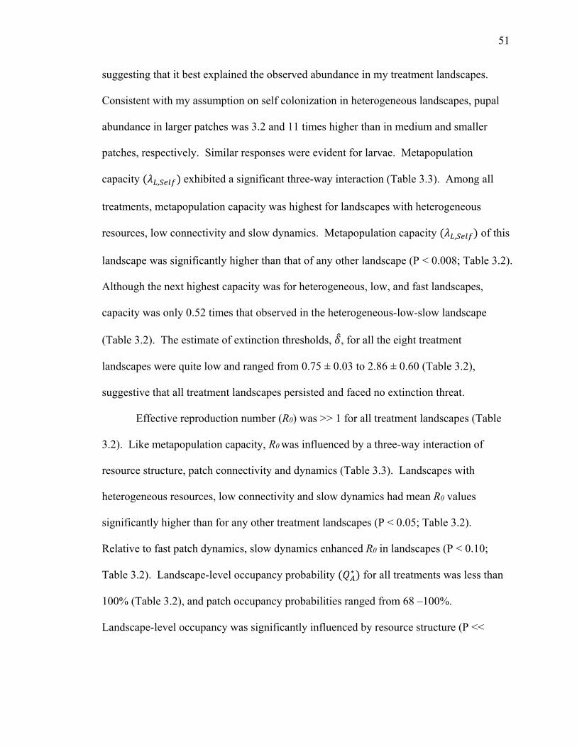
51

suggesting that it best explained the observed abundance in my treatment landscapes.

Consistent with my assumption on self colonization in heterogeneous landscapes, pupal

abundance in larger patches was 3.2 and 11 times higher than in medium and smaller

patches, respectively. Similar responses were evident for larvae. Metapopulation

capacity , exhibited a significant three-way interaction (Table 3.3). Among all

treatments, metapopulation capacity was highest for landscapes with heterogeneous

resources, low connectivity and slow dynamics. Metapopulation capacity , of this

landscape was significantly higher than that of any other landscape (P < 0.008; Table 3.2).

Although the next highest capacity was for heterogeneous, low, and fast landscapes,

capacity was only 0.52 times that observed in the heterogeneous-low-slow landscape

(Table 3.2). The estimate of extinction thresholds, , for all the eight treatment

landscapes were quite low and ranged from 0.75 ± 0.03 to 2.86 ± 0.60 (Table 3.2),

suggestive that all treatment landscapes persisted and faced no extinction threat.

Effective reproduction number (R0) was >> 1 for all treatment landscapes (Table

3.2). Like metapopulation capacity, R0 was influenced by a three-way interaction of

resource structure, patch connectivity and dynamics (Table 3.3). Landscapes with

heterogeneous resources, low connectivity and slow dynamics had mean R0 values

significantly higher than for any other treatment landscapes (P < 0.05; Table 3.2).

Relative to fast patch dynamics, slow dynamics enhanced R0 in landscapes (P < 0.10;

Table 3.2). Landscape-level occupancy probability ∗ for all treatments was less than

100% (Table 3.2), and patch occupancy probabilities ranged from 68 –100%.

Landscape-level occupancy was significantly influenced by resource structure (P <<

52

0.001; Table 3.3); heterogeneous landscapes (0.92 ± 0.01) had higher occupancy than

homogeneous ones (0.88 ± 0.01; Table 3.2).

The control (static) landscape experienced an initial abundance greater than that

observed for otherwise comparable landscapes with slow dynamics, followed by a rapid

temporal decline (Figure 3.3). Compared to its slow dynamic analog, abundance of

Weeks

0 10 20 30 40 50 60 70

Adu

lt B

eetle

Abu

ndan

ce

0

20

40

60

80

100

120

No TurnoverFast TurnoverSlow Turnover

Figure 3.3: Mean (± SE) abundance of adult beetles for experimental, 12-patch landscapes with heterogeneous resources, low connectivity, and either no (filled circle), fast (open circle), or slow (triangle) rates of patch turnover. Landscapes with slow turnover exhibited greater metapopulation abundance than landscapes with no turnover, and greater metapopulation persistence than landscapes with fast turnover (Table 3.2).

adults and pupae inside control patches, averaged for the latter half of the study period

[time step 8 -14], was lower by 67% and 57%, respectively; larval abundance was similar

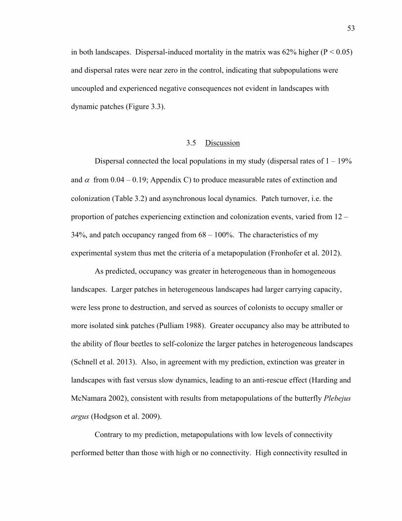
53

in both landscapes. Dispersal-induced mortality in the matrix was 62% higher (P < 0.05)

and dispersal rates were near zero in the control, indicating that subpopulations were

uncoupled and experienced negative consequences not evident in landscapes with

dynamic patches (Figure 3.3).

3.5 Discussion

Dispersal connected the local populations in my study (dispersal rates of 1 – 19%

and from 0.04 – 0.19; Appendix C) to produce measurable rates of extinction and

colonization (Table 3.2) and asynchronous local dynamics. Patch turnover, i.e. the

proportion of patches experiencing extinction and colonization events, varied from 12 –

34%, and patch occupancy ranged from 68 – 100%. The characteristics of my

experimental system thus met the criteria of a metapopulation (Fronhofer et al. 2012).

As predicted, occupancy was greater in heterogeneous than in homogeneous

landscapes. Larger patches in heterogeneous landscapes had larger carrying capacity,

were less prone to destruction, and served as sources of colonists to occupy smaller or

more isolated sink patches (Pulliam 1988). Greater occupancy also may be attributed to

the ability of flour beetles to self-colonize the larger patches in heterogeneous landscapes

(Schnell et al. 2013). Also, in agreement with my prediction, extinction was greater in

landscapes with fast versus slow dynamics, leading to an anti-rescue effect (Harding and

McNamara 2002), consistent with results from metapopulations of the butterfly Plebejus

argus (Hodgson et al. 2009).

Contrary to my prediction, metapopulations with low levels of connectivity

performed better than those with high or no connectivity. High connectivity resulted in

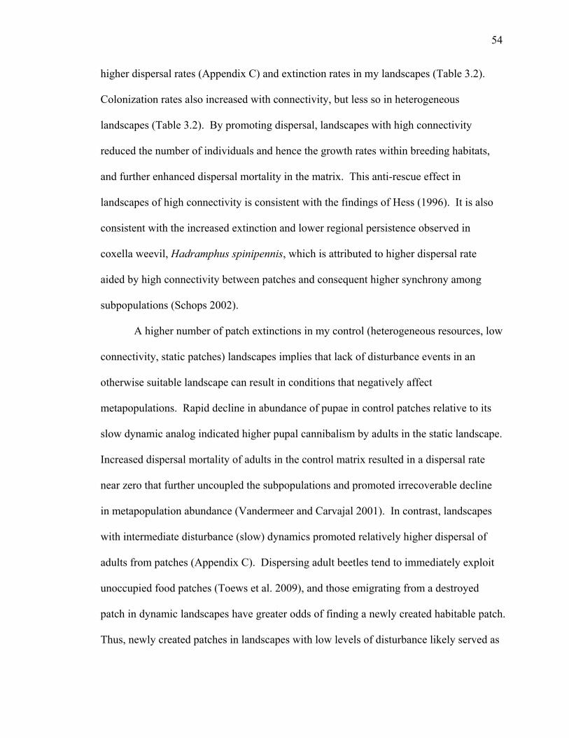
54

higher dispersal rates (Appendix C) and extinction rates in my landscapes (Table 3.2).

Colonization rates also increased with connectivity, but less so in heterogeneous

landscapes (Table 3.2). By promoting dispersal, landscapes with high connectivity

reduced the number of individuals and hence the growth rates within breeding habitats,

and further enhanced dispersal mortality in the matrix. This anti-rescue effect in

landscapes of high connectivity is consistent with the findings of Hess (1996). It is also

consistent with the increased extinction and lower regional persistence observed in

coxella weevil, Hadramphus spinipennis, which is attributed to higher dispersal rate

aided by high connectivity between patches and consequent higher synchrony among

subpopulations (Schops 2002).

A higher number of patch extinctions in my control (heterogeneous resources, low

connectivity, static patches) landscapes implies that lack of disturbance events in an

otherwise suitable landscape can result in conditions that negatively affect

metapopulations. Rapid decline in abundance of pupae in control patches relative to its

slow dynamic analog indicated higher pupal cannibalism by adults in the static landscape.

Increased dispersal mortality of adults in the control matrix resulted in a dispersal rate

near zero that further uncoupled the subpopulations and promoted irrecoverable decline

in metapopulation abundance (Vandermeer and Carvajal 2001). In contrast, landscapes

with intermediate disturbance (slow) dynamics promoted relatively higher dispersal of

adults from patches (Appendix C). Dispersing adult beetles tend to immediately exploit

unoccupied food patches (Toews et al. 2009), and those emigrating from a destroyed

patch in dynamic landscapes have greater odds of finding a newly created habitable patch.

Thus, newly created patches in landscapes with low levels of disturbance likely served as

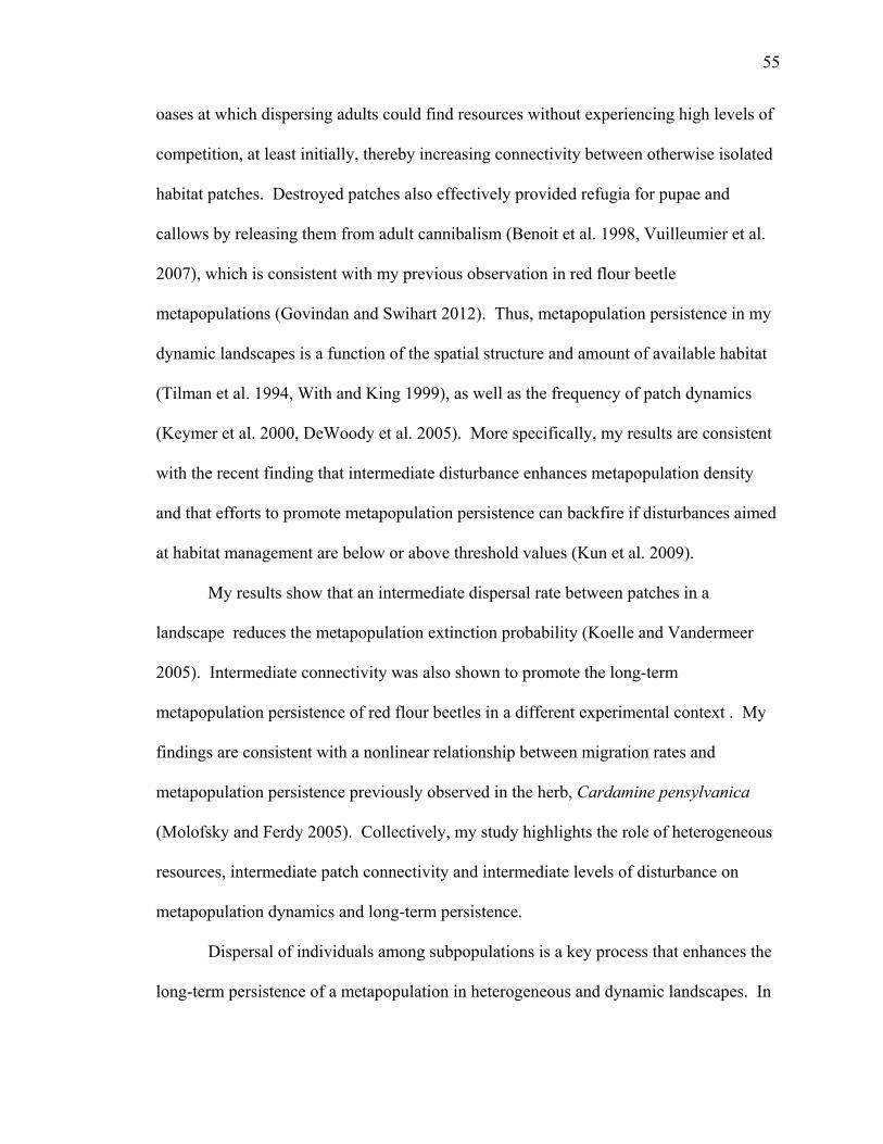
55

oases at which dispersing adults could find resources without experiencing high levels of

competition, at least initially, thereby increasing connectivity between otherwise isolated

habitat patches. Destroyed patches also effectively provided refugia for pupae and

callows by releasing them from adult cannibalism (Benoit et al. 1998, Vuilleumier et al.

2007), which is consistent with my previous observation in red flour beetle

metapopulations (Govindan and Swihart 2012). Thus, metapopulation persistence in my

dynamic landscapes is a function of the spatial structure and amount of available habitat

(Tilman et al. 1994, With and King 1999), as well as the frequency of patch dynamics

(Keymer et al. 2000, DeWoody et al. 2005). More specifically, my results are consistent

with the recent finding that intermediate disturbance enhances metapopulation density

and that efforts to promote metapopulation persistence can backfire if disturbances aimed

at habitat management are below or above threshold values (Kun et al. 2009).

My results show that an intermediate dispersal rate between patches in a

landscape reduces the metapopulation extinction probability (Koelle and Vandermeer

2005). Intermediate connectivity was also shown to promote the long-term

metapopulation persistence of red flour beetles in a different experimental context . My

findings are consistent with a nonlinear relationship between migration rates and

metapopulation persistence previously observed in the herb, Cardamine pensylvanica

(Molofsky and Ferdy 2005). Collectively, my study highlights the role of heterogeneous

resources, intermediate patch connectivity and intermediate levels of disturbance on

metapopulation dynamics and long-term persistence.

Dispersal of individuals among subpopulations is a key process that enhances the

long-term persistence of a metapopulation in heterogeneous and dynamic landscapes. In

56

a previous study with individual-based simulations (Hovestadt and Poethke 2006),

metapopulation survival was predicted to be much higher when subpopulations exhibited

density-dependent emigration as compared to density-independent emigration. This was

particularly true when dispersal rates among subpopulations ranged between 0.05 and

0.20, which reflect the rates observed in my high-connectivity landscapes. In my study,

low connectivity was achieved by manipulating the difficulty with which emigration

occurred and led to density-dependent emigration of beetles, whereas beetles in high

connectivity landscapes exhibited density-independent emigration (Appendix C).

Because adult beetles emigrated from subpopulations in landscapes with low connectivity

only at high population density, these subpopulations had lower risk of extinction due to

demographic stochasticity. In contrast, density-independent emigration in landscapes

with high connectivity resulted in higher dispersal induced mortality rates in the matrix of

these landscapes, with consequences for metapopulation performance. In heterogeneous

landscapes, beetle emigration in high-connectivity treatments corresponded with R0

values 40 – 80% lower than those observed for the low-connectivity treatments.

Similarly, metapopulation capacity was 34 – 65% lower. My results are thus consistent

with the simulations of Hovestadt and Poethke (2006) and emphasize the need to assess

the nature of density dependence of emigration for conservation planning.

My study is one of the first applications of local covariance structure to estimate

dispersal rates in coupled subpopulations, and it enabled estimation and comparison of

the metapopulation capacity of landscapes with differing spatial and temporal resource

dynamics. The simultaneous estimation of dispersal rate, local growth rate and mean

dispersal distance (Schneeberger and Jansen 2006) is less labor intensive and cheaper

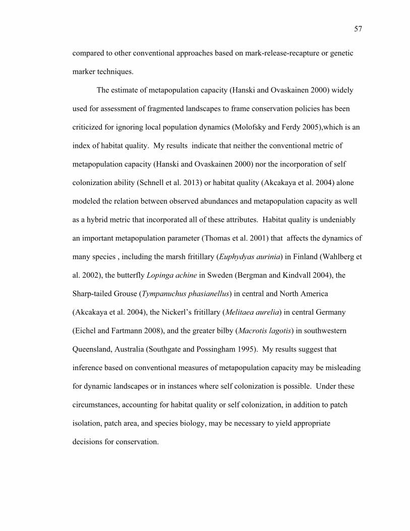
57

compared to other conventional approaches based on mark-release-recapture or genetic

marker techniques.

The estimate of metapopulation capacity (Hanski and Ovaskainen 2000) widely

used for assessment of fragmented landscapes to frame conservation policies has been

criticized for ignoring local population dynamics (Molofsky and Ferdy 2005),which is an

index of habitat quality. My results indicate that neither the conventional metric of

metapopulation capacity (Hanski and Ovaskainen 2000) nor the incorporation of self

colonization ability (Schnell et al. 2013) or habitat quality (Akcakaya et al. 2004) alone

modeled the relation between observed abundances and metapopulation capacity as well

as a hybrid metric that incorporated all of these attributes. Habitat quality is undeniably

an important metapopulation parameter (Thomas et al. 2001) that affects the dynamics of

many species , including the marsh fritillary (Euphydyas aurinia) in Finland (Wahlberg et

al. 2002), the butterfly Lopinga achine in Sweden (Bergman and Kindvall 2004), the

Sharp-tailed Grouse (Tympanuchus phasianellus) in central and North America

(Akcakaya et al. 2004), the Nickerl’s fritillary (Melitaea aurelia) in central Germany

(Eichel and Fartmann 2008), and the greater bilby (Macrotis lagotis) in southwestern

Queensland, Australia (Southgate and Possingham 1995). My results suggest that

inference based on conventional measures of metapopulation capacity may be misleading

for dynamic landscapes or in instances where self colonization is possible. Under these

circumstances, accounting for habitat quality or self colonization, in addition to patch

isolation, patch area, and species biology, may be necessary to yield appropriate

decisions for conservation.

58

CHAPTER 4. HOST SELECTION AND RESPONSES TO FOREST FRAGMENTATION IN ACORN WEEVILS: INFERENCES FROM DYNAMIC

OCCUPANCY MODELS

4.1 Abstract

Prior studies on species-specific responses to habitat alteration have demonstrated

that niche breadth is positively associated with patch occupancy rates in landscapes

fragmented by agriculture. However, these studies generally have focused on vertebrates

and relied upon data collected at a single point in time, neglecting dynamic processes that

could alter inferences. I studied the effects of host selection and forest fragmentation on

population dynamics of acorn weevils (Curculio), the primary insect seed predators of

oaks in North America. Detection/non-detection data were collected from 174 red and

white oaks in 19 forested fragments from 2005-08. I used dynamic multi-season site-

occupancy models within a Bayesian framework to explore variation in patch (tree-level)

occupancy dynamics of three species of weevils that vary in their specialization, i.e., their

relative selection of red and white oak as hosts: C. pardalis (white oak specialist), C.

sulcatulus (generalist) and C. proboscideus (generalist). Contrary to expectations, the

specialist exhibited greater estimated rates of occupancy than generalists. However, red

oak trees occupied by the white oak specialist appeared to function as sink populations

maintained by frequent colonization following local extinction. Specialists also exhibited

greater relative variation in occupancy and relative abundance on their host trees among

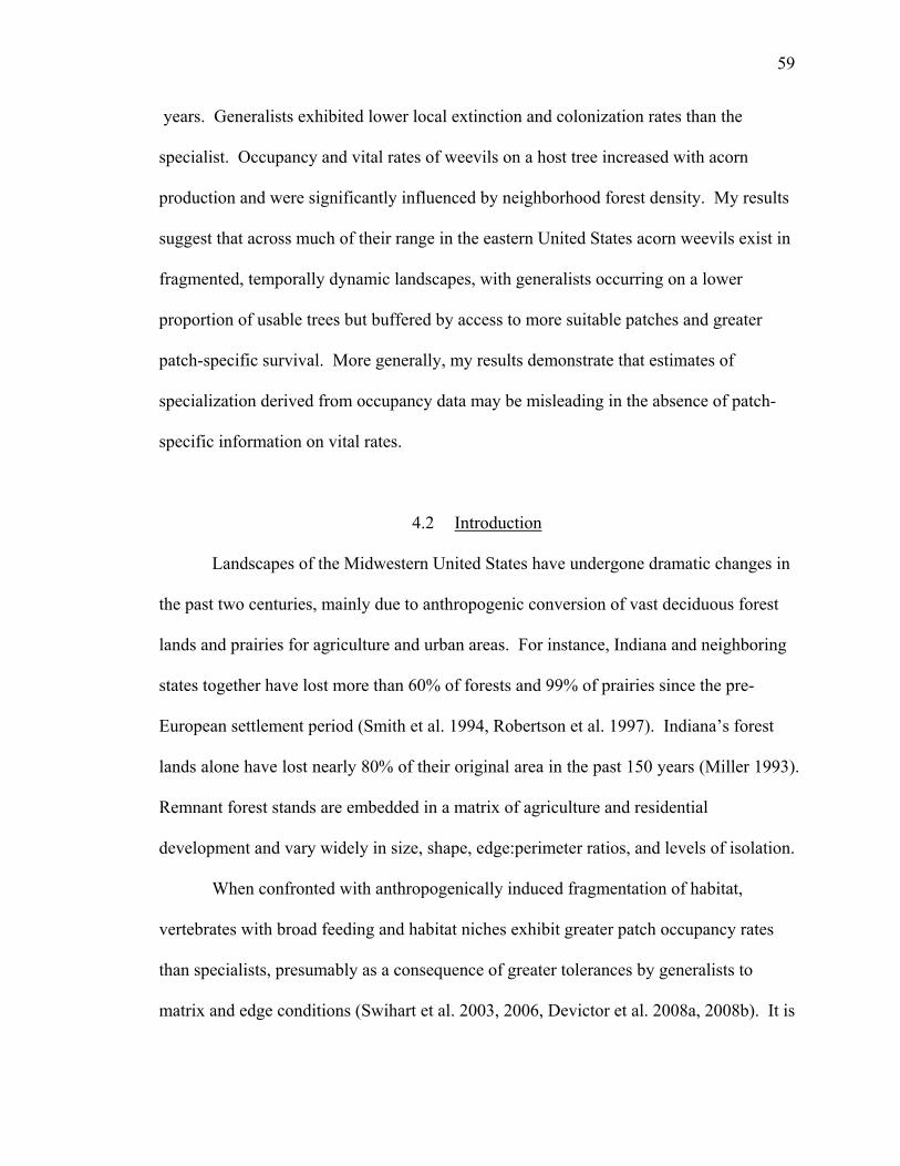
59

years. Generalists exhibited lower local extinction and colonization rates than the

specialist. Occupancy and vital rates of weevils on a host tree increased with acorn

production and were significantly influenced by neighborhood forest density. My results

suggest that across much of their range in the eastern United States acorn weevils exist in

fragmented, temporally dynamic landscapes, with generalists occurring on a lower

proportion of usable trees but buffered by access to more suitable patches and greater

patch-specific survival. More generally, my results demonstrate that estimates of

specialization derived from occupancy data may be misleading in the absence of patch-

specific information on vital rates.

4.2 Introduction

Landscapes of the Midwestern United States have undergone dramatic changes in

the past two centuries, mainly due to anthropogenic conversion of vast deciduous forest

lands and prairies for agriculture and urban areas. For instance, Indiana and neighboring

states together have lost more than 60% of forests and 99% of prairies since the pre-

European settlement period (Smith et al. 1994, Robertson et al. 1997). Indiana’s forest

lands alone have lost nearly 80% of their original area in the past 150 years (Miller 1993).

Remnant forest stands are embedded in a matrix of agriculture and residential

development and vary widely in size, shape, edge:perimeter ratios, and levels of isolation.

When confronted with anthropogenically induced fragmentation of habitat,

vertebrates with broad feeding and habitat niches exhibit greater patch occupancy rates

than specialists, presumably as a consequence of greater tolerances by generalists to

matrix and edge conditions (Swihart et al. 2003, 2006, Devictor et al. 2008a, 2008b). It is

60

unclear whether this pattern is due to increased colonization effects or enhanced local

survival, as occupancy rates have been estimated largely from single snapshots in time

that preclude inference regarding local dynamics (Moore and Swihart 2005, Rizkalla et al.

2009). Moreover, it is unclear whether this pattern generalizes to other taxa. Thus, my

primary objective was to test for an effect of niche breadth on rates of patch occupancy,

colonization, and extinction within a guild of forest insects that relies on tree seeds,

especially oaks (Quercus), as its food resource. Secondarily, I tested for effects of spatio-

temporal variability in patch quality on occupancy dynamics.

Acorn weevils (Curculio) are the primary insect seed predators of oaks and are

economically important pests. In North America they cause significant pre-dispersal loss

of acorn crops, with infestation rates ranging from 10 to 100% (Gibson 1964) and seed

mortality that can exceed 90% (Gribko 1995). Weevil-infested acorns also are less likely

to be dispersed by vertebrates such as squirrels (Sciurus) and blue jays (Cyanocitta

cristata) (Steele et al. 1996, Johnson et al. 1997). Thus, weevil abundance and

occurrence can influence acorn dispersal and survival.

Because sound acorns that serve as oviposition sites for weevils are plentiful only

in mast years, the suitability of oaks as habitat patches for breeding populations in much

of the eastern United States is temporally dynamic as well as spatially constrained to

forest stands embedded within an inhospitable matrix of agriculture and urbanization.

Considering the characteristic masting behavior of oak trees (Sork et al. 1993), the low

numbers of conspecific trees in many small forest stands (Aldrich et al. 2003; Dolan and

Swihart unpublished data), and the poorly developed dispersal ability of Curculio (Menu

1993b), it is plausible that acorn weevils in dynamic, fragmented forest landscapes are

61

likely to function as metapopulations, i.e., interconnected populations in discontinuous

habitat patches connected by migration, and whose dynamics are governed by rates of

extinction and colonization (Gilpin and Hanski 1991).

Classical metapopulation models assume that the occupancy state of a patch

(occupied or not occupied) is perfectly observable. However, this is often not likely to be

the case, since the occurrence of insect species may easily be overlooked during field

sampling even in highly standardized schemes (Gu and Swihart 2004). Hence, observed

‘absences’ may often be overlooked ‘presences’. Estimates of occupancy and rates of

colonization and extinction under classical metapopulation models are sensitive to the

assumption that there are no false absences (Moilanen 2002). Dynamic site-occupancy

models (MacKenzie et al. 2003, Royle and Kéry 2007) are extensions of classical

metapopulation models that provide unbiased estimates of the metapopulation parameters

in the face of imperfect detection.

I used dynamic site-occupancy models with covariates to explore variation in

three species of acorn weevils. Specifically, I examined the occupancy dynamics of

acorn weevils associated with their host trees in forest fragments of west-central Indiana.

In the context of the present study, each host tree was defined as a resource patch for

purposes of studying occupancy dynamics. Based on extensive sampling of Curculio

oviposition sites, Gibson (1972) concluded that C. pardalis is specialized on white oak

and occurs rarely on red oak, C. proboscideus prefers red oak and occurs sparingly on

white oak, and C. sulcatulus is found on both species. Because mast production is more

highly correlated within species of the white oak section (Lobatae) and the red oak

section (Quercus) than between species from different sections (Lusk et al. 2007),

62

generalists capable of using both sections should benefit from a larger and more

temporally reliable source of suitable oviposition sites within small forest stands. I

hypothesized that patterns of tree occupancy would reflect the differing levels of host

preferences for these species of Curculio; generalists should exhibit greater occupancy

rates on their hosts, especially during mast years, and lower rates of extinction. In

addition, I predicted that occupancy and survival of local populations should vary

positively with mast availability of host tree species, irrespective of level of

specialization. I also tested predictions regarding specific environmental factors and their

influence on occupancy dynamics of acorn weevils. When soil is dry, 27-78% of female

adult chestnut weevils (C. elephas) cannot emerge from soil and fail to reproduce (Menu

1993a). Hence, increased soil moisture in forest interiors should facilitate greater

survival and occupancy of acorn weevils on interior host trees relative to trees along

forest edges. Conversely, higher levels of canopy exposure to sunlight and release from

neighboring trees along forest edges should lead to greater seed production and attraction

of more weevils. Thus, colonization by weevils should be greater on host trees in forest

edge experiencing local extinction. Available evidence suggests that Curculio weevils

are poor dispersers (Menu 1993b). Thus, the effects of alternative host trees proximal to

a target host tree may be pronounced. Accordingly, I predicted that colonization and

occupancy should increase for host trees found within forested neighborhoods relative to

more isolated trees.

63

4.3 Methods

4.3.1 Field Sampling

To assess effects of resource availability, fragmentation, and forest structure on

seed predators, mast production and weevil occupancy were estimated annually for

individual red oak (Q. rubra) and white oak (Q. alba) in selected forest stands in

landscapes of west-central Indiana (approx. 40° 25' N / 86° 54' W). Trees of each species

were sampled in selected forest stands varying in size and isolation, with stands isolated

by distances of 0.27-56 km. Only trees >25 cm diameter at breast height (dbh) were

selected for sampling, and for each tree, diameter and height were recorded. To

determine whether forest edges influenced weevil occupancy dynamics, I stratified

selection of sampled trees as a function of distance from forest edge. For purposes of

weevil sampling, I defined edge trees as those falling within 10m of the outer perimeter

of a stand. Core trees were ≥ 30 m from the patch perimeter.

I sampled weevils from oak trees in 19 forest stands distributed evenly across 3

landscapes, each of 3-km radius and spaced 20 km apart along a gradient of declining

forest fragmentation running from Warren county to eastern Tippecanoe county. The

gradient captures the range of habitat fragmentation typically encountered in west-central

Indiana. Stands were selected to span a range of sizes and isolation commonly

encountered by weevils in the region. Along this gradient in 2005 I sampled 11 forest

stands. Within each stand I selected a maximum of three trees each of red oak and white

oak at the core and edge of the stand, depending on availability. A total of 68 trees,

consisting of 28 red oak and 40 white oak, were sampled for weevils by setting weevil

traps. Only 2 out of 11forest stands had more than three trees per species sampled in the

64

core and edge of the patches, because additional suitable forest stands with the required

number of host trees per species were unavailable for study within a radius of 3 km. I

retained the weevil traps set on all the host trees selected in 2005 until the sampling was

terminated in 2008, to repeatedly sample them for acorn weevils in successive years. For

all trees with weevil traps, estimates of mast were obtained via quadrat sampling from

2005 through 2008.

In 2006, I increased the number of forest stands sampled from 11 to 19.

Correspondingly, the total number of trees at which weevils were sampled increased from

68 to 150, with 72 trees in the edge and 78 trees in the core. I sampled weevils from 61

red oak and 89 white oak trees. Depending on the availability of the trees and tree

species composition, the number of trees per patch ranged between 3 and 18. In 2007, I

again increased the number of trees for which weevils were sampled, from 150 to 174, by

setting traps on 24 more trees in 6 of the previously selected forest stands with the goal of

attaining greater sampling intensity within each stand. The 6 forest stands selected in

2007 were distributed evenly along the gradient of fragmentation represented by the three

study landscapes. Thus by 2007, I had 74 red oak and 100 white oak trees on which

weevil traps were set, of which 94 and 80 were core and edge trees, respectively

(Supplementary material Appendix D).

The landscape context of each tree was quantified using geographic information

system (GIS) layers derived from the National Land Cover Pattern Database (Riitters et

al. 2000). These layers were derived by applying a moving window analysis to 30 m

resolution classified Landsat TM data (Loveland and Shaw 1996). For each pixel in the

land cover map, the layers quantified neighborhood forest density (FD100) in a square

65

window of 2.3 ha, corresponding to a spatial neighborhood of about 100 m around each

tree. Forest density was calculated as the proportion of forest cover pixels in the window.

Landscape characteristics were attributed to each tree by collecting tree coordinates to a

minimum accuracy of ±10 m using a handheld GPS unit, and then overlaying these

coordinates with the relevant maps. All of the above analyses were performed in ArcGIS

9.2 (ESRI 2006).

Most (60-80%) adult pecan weevils (Curculio caryae) emerging from their pupal

cells in soil walk to the bole of host trees and climb rather than fly to ascend (Cottrell and

Wood 2008). Hence, I constructed and deployed passive circle traps to capture adult

weevils emerging from soil under each tree in each of the selected forest stands. The

design of circle traps, made of aluminium insect screening, was similar to the one

described by Mulder and co-workers (2000). Two circle traps were deployed per tree

throughout the period of acorn fall in 2005 and 2006; one trap facing south and another

facing north. A circle trap was attached to a tree bole at breast height and acted as a

passive funnel that captured insects walking up the bole of the tree. In most forest stands,

trees of excessively large diameter (>30 cm dbh; larger than can be covered by 2 traps)

were sampled only when necessary to attain the minimum target of 3 trees each of a

particular host species at the forest edge and interior. Attachment of circle traps to the

trees was accomplished by using 4.1 cm exterior drywall screws (2) through pre-drilled

holes. The screen skirt was attached to the trees using 1.4 cm staples. Adult weevils

were collected from each trap every 2 weeks, labeled with tree ID and sampling date and

preserved in 95% ethanol in vials kept at -20°C. Sampling was conducted from 5

October to 2 December in 2005, 26 September to 1 December in 2006, 15 September to 7

66

November in 2007, and 11 August to 14 November in 2008. Sampling was stopped

earlier in 2007 and 2008, because few adults of any Curculio species emerged in the later

sampling periods associated with the onset of substantial declines in temperature. The

total number of biweekly visits to a tree varied from 5 in 2005 to 7 in 2008. Sampled

weevils were identified to species based on external morphological characters, using

genital dissection as needed (Gibson 1969, Downie and Arnett 1996).

I used quadrat sampling to estimate the average acorn production per trapped tree

with counts from two 1/2 m2 grids beneath trees on each sampling date. In addition to

recording survey-specific covariates (year, date of visit and acorn production),

information on different tree-specific covariates like tree species identity, tree location

(core or edge class), dbh of tree and forest density at 100 m spatial resolution was used in

occupancy models.

4.3.2 Occupancy Modeling

I adapted the hierarchical site occupancy model developed by Royle and Kéry

(2007) to make inferences about the multi-season tree occupancy dynamics of Curculio

weevils, as well as the factors affecting dynamics, using detection/non-detection data

collected from 2005-2008. Modeling of tree occupancy dynamics relies on sampling in T

seasons (primary periods), with J ≥ 2 replicate surveys at trees within a season

(secondary periods). Within a season, the occupancy status of each tree is assumed to be

unchanged (i.e. assumption of population closure). Detection of the target species during

sampling occasion j results in a detection value of 1 being recorded, whereas a 0 is

recorded if sampling fails to yield detection at the tree. Note that detection indicates

occurrence, but non-detection does not imply non-occurrence unless the probability of

67

detecting a species at a tree during sampling is one. In most instances, detection is

imperfect; i.e., a species may occur at a tree but not be detected there during any

particular sampling occasion (Gu and Swihart 2004).

Hierarchical site-occupancy models enable separate inference about the sampling

(detection) process and the partially observed (latent) occupancy state (MacKenzie et al.

2002), as well as occupancy dynamics (MacKenzie et al. 2003). The description of the

occupancy dynamics is exactly as in a metapopulation model, i.e., in terms of occupancy

probability and its rate of change due to colonization and extinction. However, this

model component is augmented by another model component which describes the

observation process. Following Royle and Kéry (2007), let z(i,t) be the true occupancy

status of tree i during primary period t, with z = 1 designating occurrence and z = 0

designating non-occurrence. Note that Ψt is the probability of tree occupancy at time t,

i.e., Ψt = Pr(z(i,t) = 1). The observed detection (or non-detection) during sampling

occasion j for tree i at primary period t is represented by Yj(i,t). Occupancy dynamics

based on the Yj(i,t) observations can be described within a hierarchical framework that

combines the observation process conditional on the true underlying occupancy state.

Initial occupancy states of the M trees are assumed to be independent, identically

distributed Bernoulli random variables with parameter Ψ1, i.e., z(i,1) Bernoulli(Ψ1), i =

1, 2, …, M. Occupancy in all subsequent primary periods (t) also is a Bernoulli random

variable that depends on the occupancy state of the tree during each previous (t-1)

primary period and the period-specific probabilities of survival ( ) and colonization ( )

(Royle and Dorazio 2008):

68

, | , 1 Bernoulli , for t = 2, 3, …, T,

where

, , 1 1 , 1 .

Thus, when a tree is occupied at 1, , 1 1 and 1 , 1 0, and the

survival component of the Bernoulli parameter is operative. In contrast, when a

tree is unoccupied at 1, , 1 0and 1 , 1 1, and the

colonization component becomes operative.

The observation model is another Bernoulli process that is specified conditional

on the latent state , :

, | , ~Bernoulli ,

In words, if tree i is occupied by the species at time t, the species will be observed with

probability pt. If tree i is unoccupied during t, Yj(i,t) = 0 (because , 0).

Heterogeneity in all model parameters (p, Ψ1, and ) can be incorporated easily as

functions of environmental or sampling covariates. For instance, the relationship

between initial occupancy (Ψ1) and covariates (Xi) can be modeled in a linear-logistic

regression as logit(Ψ1) = β0 + βi Xi, where β are parameters to be estimated.

Estimates of occupancy probability for all years after the first were obtained

recursively as 1 (Royle and Dorazio 2008).

I analyzed the dynamic site occupancy models within a Bayesian framework and

for all three Curculio species separately. When dealing with hierarchical data, a

Bayesian approach is advantageous because its computational methods are numerically

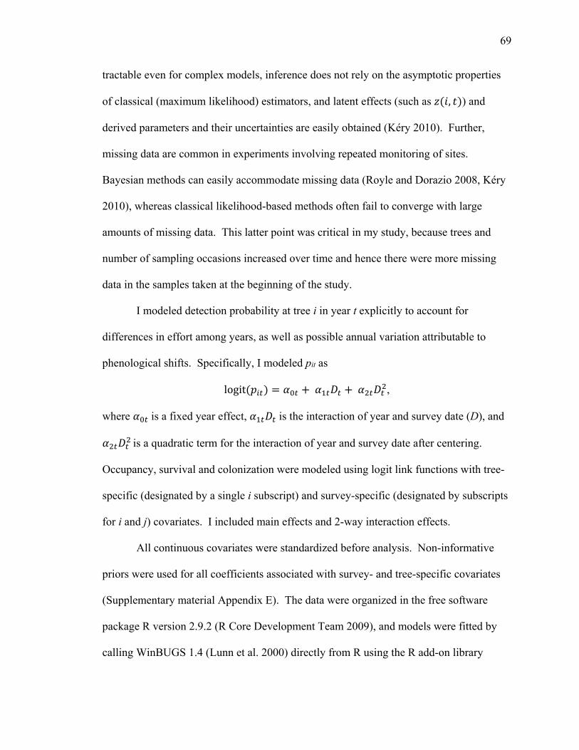
69

tractable even for complex models, inference does not rely on the asymptotic properties

of classical (maximum likelihood) estimators, and latent effects (such as , ) and

derived parameters and their uncertainties are easily obtained (Kéry 2010). Further,

missing data are common in experiments involving repeated monitoring of sites.

Bayesian methods can easily accommodate missing data (Royle and Dorazio 2008, Kéry

2010), whereas classical likelihood-based methods often fail to converge with large

amounts of missing data. This latter point was critical in my study, because trees and

number of sampling occasions increased over time and hence there were more missing

data in the samples taken at the beginning of the study.

I modeled detection probability at tree i in year t explicitly to account for

differences in effort among years, as well as possible annual variation attributable to

phenological shifts. Specifically, I modeled pit as

logit ,

where is a fixed year effect, is the interaction of year and survey date (D), and

is a quadratic term for the interaction of year and survey date after centering.

Occupancy, survival and colonization were modeled using logit link functions with tree-

specific (designated by a single i subscript) and survey-specific (designated by subscripts

for i and j) covariates. I included main effects and 2-way interaction effects.

All continuous covariates were standardized before analysis. Non-informative

priors were used for all coefficients associated with survey- and tree-specific covariates

(Supplementary material Appendix E). The data were organized in the free software

package R version 2.9.2 (R Core Development Team 2009), and models were fitted by

calling WinBUGS 1.4 (Lunn et al. 2000) directly from R using the R add-on library

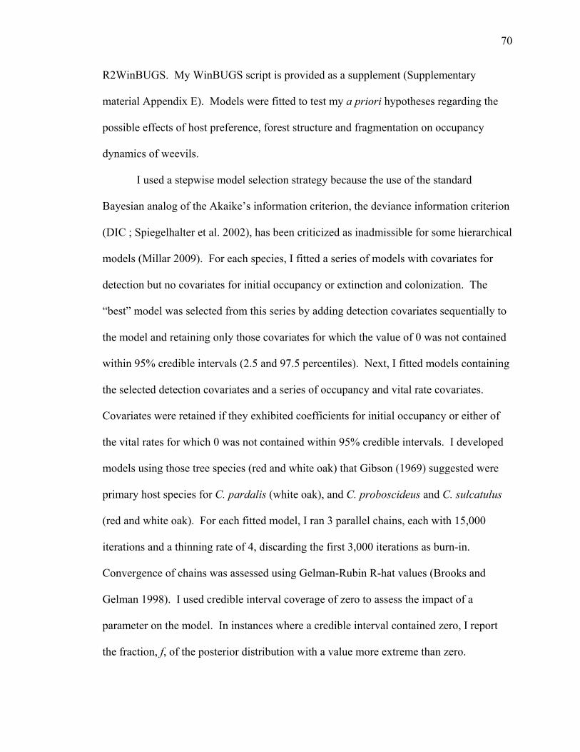
70

R2WinBUGS. My WinBUGS script is provided as a supplement (Supplementary

material Appendix E). Models were fitted to test my a priori hypotheses regarding the

possible effects of host preference, forest structure and fragmentation on occupancy

dynamics of weevils.

I used a stepwise model selection strategy because the use of the standard

Bayesian analog of the Akaike’s information criterion, the deviance information criterion

(DIC ; Spiegelhalter et al. 2002), has been criticized as inadmissible for some hierarchical

models (Millar 2009). For each species, I fitted a series of models with covariates for

detection but no covariates for initial occupancy or extinction and colonization. The

“best” model was selected from this series by adding detection covariates sequentially to

the model and retaining only those covariates for which the value of 0 was not contained

within 95% credible intervals (2.5 and 97.5 percentiles). Next, I fitted models containing

the selected detection covariates and a series of occupancy and vital rate covariates.

Covariates were retained if they exhibited coefficients for initial occupancy or either of

the vital rates for which 0 was not contained within 95% credible intervals. I developed

models using those tree species (red and white oak) that Gibson (1969) suggested were

primary host species for C. pardalis (white oak), and C. proboscideus and C. sulcatulus

(red and white oak). For each fitted model, I ran 3 parallel chains, each with 15,000

iterations and a thinning rate of 4, discarding the first 3,000 iterations as burn-in.

Convergence of chains was assessed using Gelman-Rubin R-hat values (Brooks and

Gelman 1998). I used credible interval coverage of zero to assess the impact of a

parameter on the model. In instances where a credible interval contained zero, I report

the fraction, f, of the posterior distribution with a value more extreme than zero.

71

Differences in annual occupancy and vital rates between Curculio species were also

compared directly by calculating in WinBUGS the interspecific differences for each

parameter and determining whether the 95% credible intervals contained zero.

4.3.3 Species Specialization Index

Niche breadth differences among species may result from evolutionary tradeoffs

in the ability of a species to exploit a range of resources and their capacity to use each

one. Rather than rely solely on conclusions drawn from prior studies when assessing

niche breadth, I computed species specialization index values (Julliard et al. 2006) from

occupancy data collected during the study. Specifically, I estimated adjusted indexes of

carrying capacities for each Curculio species on red and white oaks by multiplying the

posterior distributions of annual occupancy probabilities with the capture rates per tree

for the corresponding year. Within the area encompassed by my study, forest inventory

surveys conducted on 418 fixed 10 x 30 m plots from 2001 to 2003 revealed basal areas

of 165.3 and 98.7 m2/ha for stems of red oak and white oak >5 cm in diameter,

respectively (Dolan and Swihart, unpublished data). Adjusted carrying capacities on red

and white oak were hence further modified by multiplying the landscape level densities

of respective host tree species obtained from the forest inventory survey. The

coefficients of variation for adjusted carrying capacities on red and white oak were used

to estimate the differences in niche breadth among the species of acorn weevils.

72

4.4 Results

4.4.1 Host Selection

A total of 2467 weevils of the focal species were collected in the circle traps

during the 4 years of sampling. My capture results revealed disproportionate affinities

for host trees that are consistent with the findings of Gibson (1972, 1982) based on

oviposition sites (Supplementary material Appendix D). For the specialist, C. pardalis,

80.1% of all captures occurred on white oak and 19.9% on red oak. For C. sulcatulus,

59.5% of captures occurred on red oak and 40.5% on white oak. For C. proboscideus,

66.6% of captures occurred on red oak and 33.9% on white oak. In contrast, values of

the species specialization index averaged over 4 years were highest for the two generalist

species, C. proboscideus (0.79) and C. sulcatulus (0.77), and lowest for the specialist, C.

pardalis (0.59). The survival probability of C. pardalis was highest for white oaks

(Table 4.1). White oaks also had a positive effect on the first-year occupancy (fraction of

posterior distribution more extreme than zero, f = 0.10) and colonization probability (f =

0.05) of C. sulcatulus (Table 4.1).

4.4.2 Mast Effects

My predictions related to effects of mast production on metapopulation dynamics

generally were supported. Increasing mast availability increased survival probability of

C. pardalis at occupied trees, especially on white oaks, and colonization at unoccupied

trees (Table 4.1). These findings are consistent with the increased levels of C. pardalis

abundance noted during 2005 and 2007, years of heavy acorn production by white oaks

(Table 4.2). Increased acorn production was associated with increased first-year

occupancy and survival of the generalists, C. sulcatulus and C. proboscideus (f = 0.03

73

and 0.15, respectively) (Table 4.1). Mast production and colonization rates also were

positively related for C. sulcatulus (Table 4.1).

Table 4.1 : Posterior summaries of environmental covariates from dynamic occupancy

models fitted to detection data on acorn weevils (Curculio) from 2005 to 2008. Ninety-five percent credible intervals are given in parentheses. For each parameter, ‘Intercept’ refers to baseline probability. ‘Mast’ denotes gross acorn production by white and red oak species. ‘FD100’ is standardized forest density in 100 m radius of host tree, WO indicates host tree species, either a red oak (0) or a white oak (1) and WO*Mast is an interaction term for host tree species and acorn production. An asterisk indicates that the 95% credible interval did not contain zero, whereas a † signifies that a fraction, f, of the posterior distribution was more extreme than zero (see text). All parameters are on the logit scale.

Parameters C.pardalis C.sulcatulus C.proboscideus First-year occupancy

Intercept 5.19 (1.28–7.89)* 1.63 (-0.69–6.49) 0.39 (-2.63–2.34)

Mast 0.27 (-6.31–12.09) 6.22 (0.78–9.81) * 4.42 (-0.15–9.73) †

FD100 -0.01(-5.40–2.89) 3.22 (0.67–7.33)* -0.34 (-2.37–1.23)

WO 5.05 (-2.63–9.81) 2.67 (-1.35–7.24) † 0.09 (-2.03–5.72)

WO*Mast 2.27 (-10.77–12.42) -5.85 (-11.54–4.46) -1.16 (-8.55– 7.61)

Survival

Intercept 0.10 (-0.61– 0.98) 4.49 (1.69–9.98)* 7.21 (2.83–11.76) *

Mast 1.32 (0.42–2.67)* 4.31 (0.41–11.55)* 3.55(-1.01–10.63) †

FD100 -0.68 (-1.43– -0.08)* -0.12 (-0.85– 0.51) 0.93 (-0.25–2.01) †

WO 5.30 (1.57–9.86)* -1.19 (-7.18–3.16) -4.73 (-10.86–3.30)

WO*Mast 5.37 (-0.58–11.72) † 0.81 (-7.25–6.99) -0.43(-8.82–10.37)

Colonization

Intercept -0.55 (-6.31– 6.82) -5.27(-10.89– -0.34)* -5.18 (-11.68–0.37) †

Mast 8.28 (1.48–11.84) * 7.09 (1.85–10.97) * 4.32 (-8.43–11.47)

FD100 8.63 (3.35–11.85)* 0.67(0.17–1.33)* -0.009 (-0.50–0.43)

WO 0.81(-8.36–7.12) 4.34 (-0.79–9.96) † 4.28(-1.44–10.86)

WO*Mast 0.16(-11.33–11.38) -8.51(-11.87– -3.08) -4.26(-11.37–8.49)

74

Table 4.2 : Estimates of average (and standard deviation) nut production per 0.25 m2 by

2 species of trees sampled for acorn weevils. Tree Species 2005 2006 2007 2008 Red oak 20.29 (3.25) 17.86 (18.19) 13.01 (12.85) 0.38 (0.90)

White oak 11.18 (3.66) 4.55 (9.99) 10.14 (8.96) 5.33 (4.74)

4.4.3 Other Environmental Covariates

Neighborhood forest density increased the colonization and first-year occupancy

of C. sulcatulus, and had a positive effect on the survival probability of C. proboscideus

(f =0.05) (Table 4.1). Neighborhood forest density also increased the colonization

probability and decreased the survival probability of C. pardalis (Table 4.1). Location of

a host tree species on the edge or interior of forest had no effect on the first year

occupancy probability or vital parameters associated with any Curculio species.


Among three species of Curculio, C. pardalis displayed highest annual occupancy

probabilities and C. proboscideus displayed lowest occupancy probabilities in all years,

except in 2008 (Figure 4.1). Occupancy probabilities on white oaks were higher for C.

pardalis compared to C. sulcatulus and C. proboscideus in all years (95% credible

interval of differences did not contain zero). In contrast, occupancy probabilities on red

oaks were higher for C. sulcatulus and C. proboscideus compared to C. pardalis, except

in 2005 (Figure 4.1). C. pardalis exhibited more variable occupancy probabilities on red

oak than white oak, with marked declines on red oak in 2006 and 2008 (Figure 4.1). The

other two species showed patterns in occupancy probabilities on white oak similar to that

of C. pardalis. On red oak, occupancy probabilities of C. proboscideus and C. sulcatulus

were relatively stable (Figure 4.1).

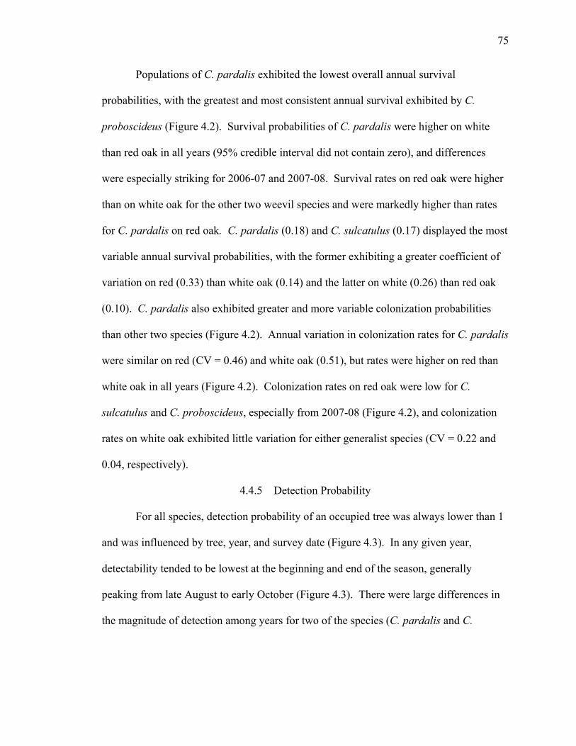
75

Populations of C. pardalis exhibited the lowest overall annual survival

probabilities, with the greatest and most consistent annual survival exhibited by C.

proboscideus (Figure 4.2). Survival probabilities of C. pardalis were higher on white

than red oak in all years (95% credible interval did not contain zero), and differences

were especially striking for 2006-07 and 2007-08. Survival rates on red oak were higher

than on white oak for the other two weevil species and were markedly higher than rates

for C. pardalis on red oak. C. pardalis (0.18) and C. sulcatulus (0.17) displayed the most

variable annual survival probabilities, with the former exhibiting a greater coefficient of

variation on red (0.33) than white oak (0.14) and the latter on white (0.26) than red oak

(0.10). C. pardalis also exhibited greater and more variable colonization probabilities

than other two species (Figure 4.2). Annual variation in colonization rates for C. pardalis

were similar on red (CV = 0.46) and white oak (0.51), but rates were higher on red than

white oak in all years (Figure 4.2). Colonization rates on red oak were low for C.

sulcatulus and C. proboscideus, especially from 2007-08 (Figure 4.2), and colonization

rates on white oak exhibited little variation for either generalist species (CV = 0.22 and

0.04, respectively).

4.4.5 Detection Probability

For all species, detection probability of an occupied tree was always lower than 1

and was influenced by tree, year, and survey date (Figure 4.3). In any given year,

detectability tended to be lowest at the beginning and end of the season, generally

peaking from late August to early October (Figure 4.3). There were large differences in

the magnitude of detection among years for two of the species (C. pardalis and C.

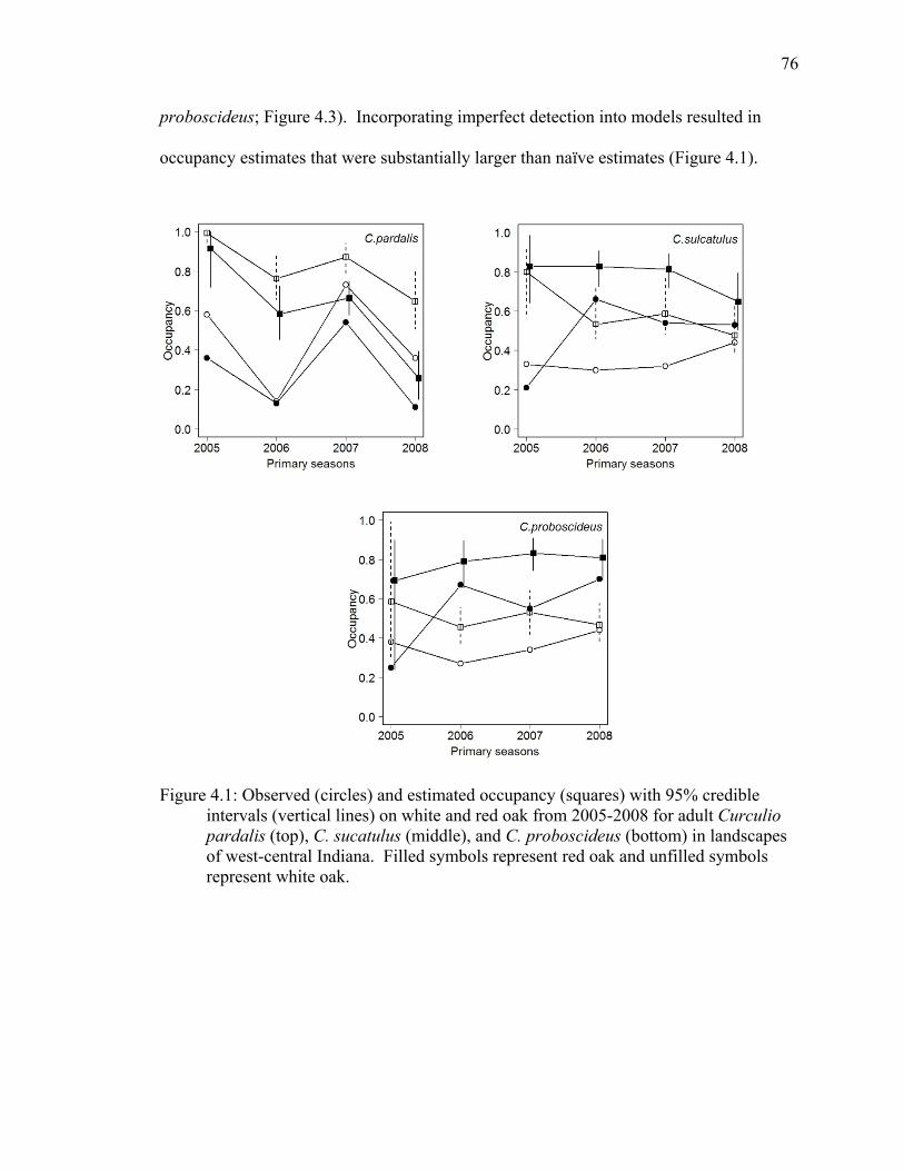
76

proboscideus; Figure 4.3). Incorporating imperfect detection into models resulted in

occupancy estimates that were substantially larger than naïve estimates (Figure 4.1).

Figure 4.1: Observed (circles) and estimated occupancy (squares) with 95% credible intervals (vertical lines) on white and red oak from 2005-2008 for adult Curculio pardalis (top), C. sucatulus (middle), and C. proboscideus (bottom) in landscapes of west-central Indiana. Filled symbols represent red oak and unfilled symbols represent white oak.

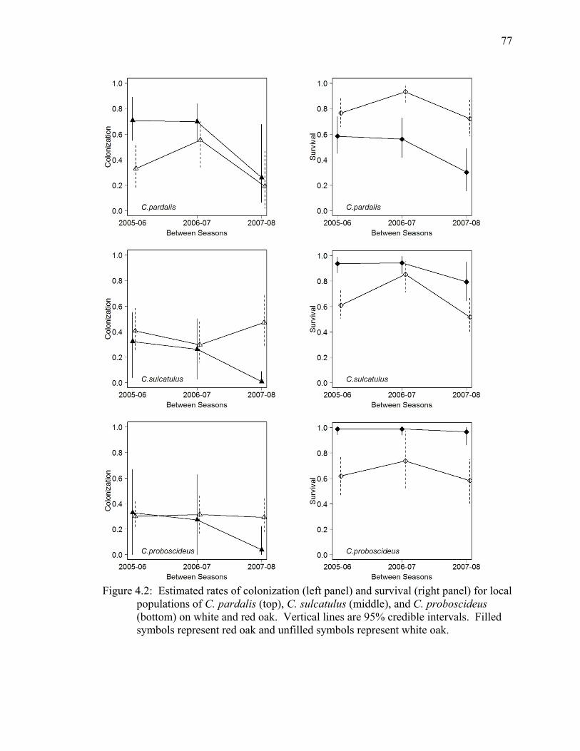
77

Figure 4.2: Estimated rates of colonization (left panel) and survival (right panel) for local

populations of C. pardalis (top), C. sulcatulus (middle), and C. proboscideus (bottom) on white and red oak. Vertical lines are 95% credible intervals. Filled symbols represent red oak and unfilled symbols represent white oak.

78

Figure 4.3: Season and survey-specific estimates of detection probability for C. pardalis (top), C. sulcatulus (middle), and C. proboscideus (bottom) sampled at trees in west-central Indiana from 2005 (solid line), 2006 (dotted line), 2007 (dashed-dotted line), and 2008 (dashed line).

4.5 Discussion

4.5.1 Effects of Fragmentation and Host Preferences on Weevil Dynamics

Degradation of landscapes has been linked to communities dominated by

generalists, presumably in response to human-induced selection gradients that favor

species adapted to survive in modified ecosystems (Devictor et al. 2008a). Based solely

on estimated occupancy rates, my results for acorn weevils seem to contradict this more

79

general pattern; the species with the narrowest host requirements, C. pardalis, exhibited

annual occupancy rates exceeding or equaling those of the more generalist species

(Figure 4.1). However, this overly simplistic characterization fails to consider the

availability of host resources, a common problem with metrics of specialization based on

the realized Grinnellian niche (Devictor et al. 2010). Higher basal areas for stems of red

(165.3 m2/ha) than white oak (98.7 m2/ha) across the landscape reveal that C. pardalis

had a suitable resource base (white oak) that was only 37.3% of the resource available to

the other two more generalist weevil species capable of using white and red oak. For a

landscape of a given size, a smaller set of available patches increases the importance of

each local population to the stability of a metapopulation. In this context, it is telling that

the coefficient of variation in annual occupancy for the specialist C. pardalis was 0.27,

compared with 0.16 and 0.04 for the more generalist C. sulcatulus and C. proboscideus,

respectively (Figure 4.1). In other words, C. pardalis relied on a subset of the host

resources available to the other two species, and exhibited occupancy rates that were 1.7-

6.8 times more variable from year to year. Thus, generalist species of weevils occupied

more trees and exhibited less annual variation in occupancy than specialists, which is

consistent with prior studies that have considered the role of niche breadth in community

structure of modified landscapes (Devictor et al. 2008a, b; Swihart et al. 2003, 2006).

Contrary to expectations derived from prior studies, values of the species

specialization index were lower for C. pardalis (0.59) compared to C. sulcatulus (0.77)

and C. proboscideus (0.79), suggesting that the former species was less specialized than

the others. This apparent paradox is due to an implicit assumption of the specialization

index; namely, that occupancy reflects suitability. As noted by Van Horne (1983), local

80

density may provide a misleading characterization of the actual quality of a habitat in

terms of its carrying capacity. Ideally, information on local birth and death rates is also

used to provide a direct assessment of suitability in terms of population growth rate. In a

metapopulation colonization and extinction become the rates of interest, because they

provide information on the quality of patches in terms of average fitness. In this context,

the occupancy patterns of C. pardalis (Figure 4.1) appear to reflect source-sink dynamics

between white (source) and red (sink) oak. C. pardalis compensated for lower survival

rates on red than white oak with high colonization rates on to red oak (Figure 4.2). Thus,

elevated levels of occupancy reflected repeated colonization of local populations

following local extinction on low-quality red oak. By comparison, the other two weevil

species exhibited higher survival rates on their primary host (red oak) and lower

extinction rates on their secondary host (white oak), but a diminished capacity for

colonization of patches following extinction (Figure 4.2). In short, C. pardalis appears to

be more specialized on its primary host but a better colonist following extinction than the

other two species. The latter point is consistent with Gibson (1969) but not with results

from the species specialization index. By focusing solely on occurrence and abundance,

the specialization index fails to account for differences in the likely source of individuals

(in situ recruit or colonist) among host trees. Future attempts to estimate specialization

across patches would benefit from explicitly incorporating vital rates or other

performance measures for local populations (see Van Horne 1983).

Ultimately, occupancy of a patch reflects the interplay of local extinction and

colonization. Predictably, the greatest generalist, C. sulcatulus, exhibited the least

variable rates of colonization during the study, reflecting reduced sensitivity to years of

81

low mast production in either red or white oak. In contrast, colonization rates of C.

pardalis declined in the poor white oak years of 2006 and 2008, and colonization rates of

C. proboscideus dropped in the poor red oak year of 2008 (Figure 4.2, Table 4.2).

Acorns of white and red oak mature in 1 and 2 years, respectively, and negative

correlations in mast production have been noted on numerous occasions for oak species

that differ in acorn maturation schedules (Koenig and Knops 2002). Thus, generalist

weevils like C. sulcatulus experience lower likelihoods of complete host failure in any

given year than more specialized species.

Site occupancy in heterogeneous landscapes is predicted best by the occupancy

status of neighboring patches, presumably because of rescue effects from dispersal

(Hanski and Gyllenberg 1993). A corollary of this finding is the expectation that

conditions leading to an increased probability of occurrence in a neighboring patch will

promote occupancy of a target patch (Prugh 2009). For Curculio weevils in my study,

neighboring patches (trees) typically are found within a forest fragment. In small

fragments, few conspecific trees occur. Thus, rescue effects from neighbors should be

enhanced for Curculio that are able to use multiple host species, yielding a predicted

ordering of extinction rates as C. sulcatulusC. proboscideus<C. pardalis. Models

supported this prediction, with C. pardalis demonstrating the highest extinction rates, and

similar but lower values for C. sulcatulus and C. proboscideus (Figure 4.2). Differences

in dispersal ability or diapause behavior may explain variation not caused by degree of

host specialization. Variability in diapause behavior and hence life cycle duration is an

adaptation to yearly and unpredictable variability in masting of host trees (Maeto and

Ozaki 2003). My results for colonization suggest that C. pardalis may exhibit greater

82

dispersal ability than the other two species, thereby compensating somewhat for effects

of fragmentation and variable patch suitability leading to local extinction. C. pardalis

also may benefit from prolonged diapause and cues enabling plasticity in breaking

diapause. Because acorns of white oak mature in a single year, weather cues during the

growing season (e.g., precipitation, temperature) may serve as reliable indicators of acorn

production (Lusk et al. 2007) and hence favor emergence of adult C. pardalis from the

soil. Clearly, variation in dispersal and diapause behavior among Curculio warrants

investigation as a factor capable of generating divergent dynamics. Indeed, if prolonged

diapause occurs in my study species, lack of breeding adults in a habitat need not imply

local population extinction, as extant weevil larvae may persist below the soil surface.

Similarly, recolonization of an apparently unoccupied patch in a subsequent season may

occur by emergence of resident weevils in situ, rather than by dispersal from other

patches. In this regard, prolonged diapause is functionally equivalent to a seed bank that

enables dispersal through time as well as space (Bullock et al. 2002).

4.5.2 Modeling Dynamics when Detection is Imperfect

Previously, field monitoring of insect pest populations to estimate abundance or

occurrence generally have ignored imperfect detection (Royama et al. 2005) by not

differentiating non-detection from absence (Sileshi 2007, Kéry et al. 2009, Dorazio et al.

2010), leading to biased and less accurate parameter estimates (Gu and Swihart 2004). I

have demonstrated with an insect case study the utility of models that account for

imperfect detection through spatially and temporally replicated surveys to improve

inference regarding population dynamics (Royle and Dorazio 2008).

83

Detection probabilities varied markedly among species, years, and surveys,

mostly due to variation in abundance. Detection probability for C. pardalis was high

throughout the surveys in 2005 and 2007, and that for C. proboscideus was high in 2006

on red oak, its primary host (Figure 4.3). Increased detectability was thus consistent with

increased abundance of particular Curculio species in response to increased mast

availability of primary hosts in corresponding years. Concurrently, year-specific

apparent occupancy rates (Figure 4.1) were more strongly negatively biased for all

species when detection probability was low. Inter-annual and intra-annual variation in

detection probability for all 3 Curculio species (Figure 4.3) can be attributed to variation

in abundance and time of emergence of each species and agree with similar observations

for butterflies and other organisms (Pellet 2008). Indeed, the seasonal curves of detection

probability arguably can be interpreted as flight periods or curves depicting the

approximate relative abundance of each species in a year. For models with all host tree

species, increases in detectability were highest with lowest trap captures, an indication of

the utility of this modeling framework for confirming the presence of even rare or

difficult-to-find species at study sites with minimal effort (Kéry 2010). Obviously, the

rich patterns in detection probability of Curculio (among species, years, and seasons)

emphasize the importance of formally accounting for imperfect detection in analyses of

insect population dynamics to enable unbiased comparisons of occupancy, survival and

colonization rates.

An additional benefit of the modeling framework I used is the ability to

incorporate covariates as a means of testing the effects of environmental factors on

occupancy and vital rates. Most importantly, by accounting for detection probability, this

84

modeling framework reduces bias in the slope estimate of the relationship between

occurrence probability and covariates (Gu and Swihart 2004), thereby enabling more

precise estimation of parameters.

I have shown that repeated sampling at multiple sites enables broader questions

pertaining to population and community dynamics to be addressed with little change in

traditional sampling protocols. Site-occupancy models provide a formal and flexible

framework for separately modeling the true metapopulation dynamics (i.e., occupancy,

survival, colonization and turnover rates) and the key parameter of the detection process

(detection probability). Moreover, all parameters can be modeled in a logistic regression

manner, as a function of covariates, to test for covariate relationships and for improved

precision of estimates. Hence, site-occupancy models are likely to yield much-improved

inferences about insect population dynamics compared to traditional approaches that

confound the true state (occupancy and its dynamics) with the observation process

(represented by imperfect detection).

4.6 Conclusion

Niche specialization can be costly in highly disturbed landscapes, and habitat

fragmentation can exacerbate these costs by creating discontinuities in suitable habitat

that increase a species’ reliance on dispersal. Occupancy commonly has been used as a

measure of relative tolerance to disturbance within a community (Devictor et al. 2008b).

In my study, though, a clear understanding of the landscape-scale effects of specialization

necessitated consideration of occupancy, availability, and temporal variation in vital rates.

Indeed, most landscape-level analyses of the role of life history or ecological attributes

85

would benefit from a broader view of species’ tolerances. Fortunately, a broader view

can be accommodated fairly easily within the framework of multi-season dynamic

occupancy models. For acorn weevils, the more specialized species experienced

increased occupancy of primary host trees but a dramatically reduced number of suitable

hosts. A reduced level of population stability resulted, as C. pardalis was not buffered by

the vagaries of acorn production in its white oak host to the same extent as the more

generalist C. proboscideus and C. sulcatulus. Greater rates of local extinction in C.

pardalis were offset at least partly by greater rates of colonization. Although none of the

weevil species considered in my study is in danger of metapopulation extinction,

continued habitat loss (Abrams 2003) likely poses a greater risk to the most specialized

member of the guild.

86

CHAPTER 5. COMMUNITY STRUCTURE OF ACORN WEEVILS IN RELATION TO DYNAMICS OF NUT PRODUCTION: INFERENCES FROM MULTI-

SPECIES OCCURRENCE MODELS

5.1 Abstract

I tested whether community structure in acorn weevils (Curculio) is influenced by

spatio-temporal variation in mast availability on host tree species. Mast production and

weevil occupancy were estimated annually from 2006-2008 for individual host trees in a

sample of 74 red oaks (Quercus rubra), 100 white oaks (Q. alba) and 84 shagbark

hickories (Carya ovata). The host trees were sampled from nineteen fragmented forest

stands in west-central Indiana, USA. Yearly estimates of site-specific occupancy,

survival and colonization of nine Curculio species on their primary host tree(s) species

were derived using multi-species, multi-season (MSMS) models within a Bayesian

framework that accounted for imperfect detection. Species richness and community

similarity estimates for corresponding years were derived from site occupancies, and

patterns were compared against annual variation in mast production. Mast production

had a strong positive effect on community-level occupancy and patch survival of

Curculio weevils. Mean weevil species richness per tree and community similarity were

highest in 2007 when mast production on all host tree species were in phase. Parameter

estimates from MSMS models were more precise than those from single-species models.

87

My results suggest that differential suitability of hosts as resources for weevil species

created a spatial storage effect that, coupled with a temporal storage effect induced by

prolonged diapause in Curculio, facilitated their coexistence. Both storage effects were

more pronounced for generalist species that evinced source (red oak)–sink (white oak)

dynamics. Coexistence peaked when all of the host tree species produced mast,

maximizing the spatio-temporal availability of resources for consumers.

Methodologically, multi-species modeling proved superior to conventional approaches

and should generally be more useful in studies of community dynamics.

5.2 Introduction

Despite insufficient regeneration in recent decades, oaks (Quercus) and hickories

(Carya) remain co-dominant in deciduous forests throughout much of the eastern United

States (Abrams 1998, McShea and Healy 2002, Moser et al. 2006, McShea et al. 2007).

Indeed, oaks serve as foundation species by regulating the structure and dynamics of

vertebrate and invertebrate communities and stabilizing the functional diversity necessary

to maintain energy flow and nutrient recycling in hardwood ecosystems (McShea 2000,

McShea and Healy 2002, Ellison et al. 2005). Both oaks and hickories naturally

regenerate by seed and serve as habitat for a wide variety of wildlife. Insect seed

predators, as well as numerous species of birds and mammals rely on acorns as a primary

source of food during fall and winter (Kirkpatrick and Pekins 2002, McShea et al. 2007).

In turn vertebrates and invertebrates can affect dispersal and regeneration of oaks

(Marquis et al. 1976, Merritt 1979).

88

Among the multiple biotic factors that influence oak regeneration, pre-dispersal

mortality due to infestation of seed by acorn weevils (Curculio) is considered important

(Abrams 1992, Oak 2002, Abrams 2003, Espelta et al. 2009). In North America, acorn

weevils are the primary insect seed predators of oaks. They can infest 50-90% of an

acorn crop on a regular basis (Gibson 1964, Galford et al. 1998, Aldrich et al. 2003), with

>90% mortality of infested seed possible (Gribko 1995).

Oaks and hickories exhibit episodic masting (Koenig and Knops 2002, Lusk et al.

2007), perhaps to counter weevils and other agents of mortality and enhance their natural

regeneration from seeds (Kelly 1994). Mast seeding is characterized by intermittent and

synchronized production of large seed crops among conspecific or co-occurring species

of trees, separated by several intervening years of small seed crops (Kelly 1994, Kelly

and Sork 2002). Most acorns produced in non-mast years are consumed by vertebrate

and invertebrate wildlife (Sork 1993). In years of poor acorn production, infestation rates

by acorn weevils tend to increase (Venner et al. 2011, Kellner et al. 2012, Kellner et al. In

Press). Mast seeding can satiate both invertebrate and vertebrate seed predators and

thereby increase acorn survival to germination (Steele and Smallwood 2002, Haas and

Heske 2005, Moore and Swihart 2007). Acorns infested by acorn weevils are not

preferred by scatter-hoarding mammals and jays, further reducing seed dispersal (Steele

et al. 1996, Dixon et al. 1997, Jones et al. 1998). Thus, acorn weevil abundance may

influence acorn dispersal, survival and oak regeneration.

Previous studies have investigated how mast seeding alters community structure

in oak-dominated forests through its cascading effects on population densities of various

invertebrate and vertebrate species at multiple trophic levels (Ostfeld et al. 1996).

89

However, few studies have examined the relation between mast production in oaks and

hickories and infestation by acorn weevils (Crawley and Long 1995, Maeto and Ozaki

2003) and its implications for community assemblages of weevils (Venner et al. 2011).

Venner et al. (2011) examined population dynamics in four species of acorn weevils

occupying two isolated host trees (Q. robur and Q. petraea) in France. They observed

differences among the weevil species in terms of their population dynamics and

responses to acorn production. Both of the oaks in their study belonged to the section

Lobatae and thus were likely to have exhibited greater temporal covariation in mast

production than more phylogenetically distinctive pairings (Lusk et al. 2007). I extended

the work of Venner et al. (2011) by investigating the community structure and occupancy

dynamics of acorn weevils in relation to spatial and temporal habitat heterogeneity

imposed by variation in mast availability for oaks from different sections, as well as a

species of hickory.

In much of the Midwestern U.S., oaks and hickories occur spatially as isolated

resource patches for acorn weevils in forests fragmented by agriculture and urban

development, and numbers of conspecific trees in most small forest stands are very low

(Aldrich et al. 2003, Swihart and Dolan Unpublished Data). Weevil populations in these

settings should exhibit patterns of host-tree occupancy that reflect their niche breadth and

the spatio-temporal dynamics in availability and suitability of mast resources (Govindan

et al. 2012). Of the 9 Curculio species in my study area, four show higher affinity for

white oak (C. pardalis, C. confusor, C. iowensis and C. strictus), two show higher

affinity for red oak (C. nasicus and C. orthorhynchus), two are generalists on white oak

and red oak (C. sulcatulus and C. proboscideus); and one (C. caryae) relies on hickory as

90

a primary host (Gibson 1969). Specifically, I predicted that when mixed hardwood forest

stands dominated by red oak (Q. rubra), white oak (Q. alba) and shagbark hickory (C.

ovata) are in phase with regard to mast seeding, patch survival, occupancy, species

richness and hence community similarity of Curculio species should be higher than when

all or some of these tree species experience simultaneous seed crop failure. From a

population perspective, I similarly predicted an increase in survival and occupancy of

Curculio in years when both red and white oak produced good seed crops.

I also predicted that survival, colonization and occupancy for weevil species

should be lower on a non-masting host species than on a masting host, and this effect

should be more pronounced for specialists than generalists. Consequently, I predicted

that species richness in a given year should be higher on a host tree species when masting

relative to an alternative non-masting host species. Further, when considered between

years, species richness on any given host tree species should be higher in a mast year

relative to a non-mast year. Accordingly, assemblage similarity of Curculio weevils

between two host tree species should be highest when both species are masting.

5.3 Materials and Methods

5.3.1 Study Area and Study Species

To assess the effect of resource availability on the species richness and

community composition of acorn weevils, mast production and weevil occupancy were

estimated annually for individual red oak, white oak, and shagbark hickory in selected

forest stands in landscapes of west-central Indiana (approx. 40° 25' N / 86° 54' W). With

one exception, Curculio species considered in my study are not expected to breed on

91

hickory and should exhibit higher occupancy on oaks. However, estimating occupancy in

both focal and surrounding non-focal habitats can help in identifying impacts of habitat

loss and fragmentation on species (Ruiz-Gutierrez et al. 2010). Hence, I included

shagbark hickory in the survey since oaks and hickories are interspersed in fragmented

forests of west-central Indiana and hickories are known hosts of Curculio caryae

(Mynhardt et al. 2007).

5.3.2 Field Sampling

Trapping of acorn weevils (Curculio) on host trees was conducted from 26

September to 1 December in 2006, 15 September to 7 November in 2007, and 11 August

to 14 November in 2008. Selection of the landscapes, fragmented forested stands within

them, selection of host trees in those forest stands, design of circle traps, sampling and

processing of weevils and quadrat sampling for mast estimation are detailed elsewhere

(Govindan et al. 2012). Briefly, I selected 19 forest stands along an east-west gradient of

habitat fragmentation in Warren and Tippecanoe counties. Within these stands two

passive circle traps (Mulder et al. 2000) were installed at breast height on 74 red oak, 100

white oak, and 81 shagbark hickory, roughly evenly distributed between edge and interior

locations (Table 5.1). Trees were visited biweekly on 5-8 occasions each autumn to

collect adult weevils, which were preserved in 95% ethanol and identified based on

morphological and anatomical characters (Gibson 1969, Downie and Arnett 1996).

5.3.3 Occupancy Modeling

Because acorn weevils exhibit poor dispersal ability (Raney and Eikenbary 1968,

Menu 1993b, Menu and Debouzie 1993), it is plausible to characterize their host trees as

patches (Govindan et al. 2012) and model acorn weevils in dynamic, fragmented forest

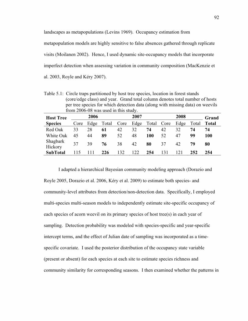
92

landscapes as metapopulations (Levins 1969). Occupancy estimation from

metapopulation models are highly sensitive to false absences gathered through replicate

visits (Moilanen 2002). Hence, I used dynamic site-occupancy models that incorporate

imperfect detection when assessing variation in community composition (MacKenzie et

al. 2003, Royle and Kéry 2007).

Table 5.1: Circle traps partitioned by host tree species, location in forest stands

(core/edge class) and year. Grand total column denotes total number of hosts per tree species for which detection data (along with missing data) on weevils from 2006-08 was used in this study.

Host Tree Species

2006 2007 2008 Grand Total Core Edge Total Core Edge Total Core Edge Total

Red Oak 33 28 61 42 32 74 42 32 74 74 White Oak 45 44 89 52 48 100 52 47 99 100 Shagbark Hickory

37 39 76 38 42 80 37 42 79 80

SubTotal 115 111 226 132 122 254 131 121 252 254

I adapted a hierarchical Bayesian community modeling approach (Dorazio and

Royle 2005, Dorazio et al. 2006, Kéry et al. 2009) to estimate both species- and

community-level attributes from detection/non-detection data. Specifically, I employed

multi-species multi-season models to independently estimate site-specific occupancy of

each species of acorn weevil on its primary species of host tree(s) in each year of

sampling. Detection probability was modeled with species-specific and year-specific

intercept terms, and the effect of Julian date of sampling was incorporated as a time-

specific covariate. I used the posterior distribution of the occupancy state variable

(present or absent) for each species at each site to estimate species richness and

community similarity for corresponding seasons. I then examined whether the patterns in

93

community parameters corresponded with variation in mast production of host trees

across the 3 years.

Hierarchical multi-species multi-season models [MSMS] are extensions of the

single-species multi-season dynamic occupancy models (Dorazio and Royle 2005,

Dorazio et al. 2006). The basic sampling design remains the same as in the case of single

species occupancy models, but detection is recorded for multiple species (n = 9 in this

study) from each site k (k = 74 for red oak, 81 for shagbark hickory, 100 for white oak,

and 255 for all host trees combined) on each visit m (secondary visits within a year,

minimum of 5 and maximum of 8) during primary period t. Population demographic

closure is assumed for each species i during each primary sampling season t, but not

between seasons.

I denote Y(i,k,m,t) as the observed data array on detection (or non-detection) for

species i at site k during sampling occasion m in primary period t. Hence Y(i,k,m,t) is a

binary variable with Y(i,k,m,t) = 1 if target species i is detected on occasion m at site k

during t, and Y(i,k,m,t) = 0 if it is not detected at site k during m in t. Non-detection

[Y(i,k,m,t) = 0] can be due either to true absence of species i at the site or due to detection

failure to detect the species even though it occurred at the site. Failure to account for

imperfect detection can confound the relation between occupancy and covariates (Gu and

Swihart 2004). Multiple visits to a site k during sampling season t can provide unbiased

information on the true site-specific occupancy state of species i with an associated

probability of detection p(i,k,m,t). Specifically, the true occupancy state of species i at

site k during primary period t is defined as another binary variable, represented by the

array z(i,k,t), with z = 1 and z = 0 indicating presence (occupancy) and absence,

94

respectively. Hierarchical modeling thus enables the true absence of a species to be

uncoupled from non-detection by allowing separate inference on the sampling (detection)

process embodied in the observation array Y and the underlying ecological process

characterized by the partially observed occupancy state z (MacKenzie et al. 2002).

A parameter of special interest in the multi-species multi-season model is

occupancy probability Ψi,k,t , i.e., the probability that species i occupies site k during

primary period t. Provided that at least a few sites are occupied by species i in the first

primary period (t=1), initial occupancy z(i,k,1) for each species i and site k is modeled as

the outcome of a Bernoulli trial,

z(i,k,1)| Ψi,k,1 Bernoulli(Ψi,k,1) .

The observed data Y(i,k,m,t) is conditional on the latent state z(i,k,t). Specifically, when

site k is occupied by species i at primary period t =1, i.e. z(i,k,1) = 1, then species i will

be observed [Y(i,k,m,1) = 1] with detection probability p(i,k,m,1). Otherwise, the

observed datum is either a fixed or sampling zero. Y(i,k,m,1) is a fixed zero if site k is

unoccupied by species i during t =1 (i.e. true absence, z(i,k,1) =0)]. Y(i,k,m,1) is a

sampling zero if species i is present but not detected (which occurs with probability 1 –

p(i,k,m,1)). Occupancy of species i in all subsequent primary periods (t >1) also is a

Bernoulli random variable that in turn depends on the occupancy state of the site k during

each previous (t – 1) primary period and the period-specific probabilities of survival

( , , ) and colonization ( , , ) (Royle and Dorazio 2008):

, , | , , 1 Bernoulli , , 1 , , 1 , ,

1 , , for t = 2, 3, …, T.

95

Following this, the observation model can be specified as a Bernoulli process conditional

on the latent state z(i,k,t):

Y(i,k,m,t) | (p(i,k,m,t), z(i,k,t)) ~ Bernoulli (z(i,k,t) p(i,k,m,t)) .

I also accounted for species-, site- and survey-specific heterogeneity in detection

(p(i,k,m,t)) and occupancy (Ψi,k,t) probability. In each primary season, I modeled

detection and occupancy as functions of appropriate covariates. For each species i,

detection probability at site k in year t was allowed to vary by survey date corresponding

to visit m (linear and squared terms for Julian date) to account for the phenological shifts

in Curculio emergence from soil after breaking diapause, and also by year t of the survey

to account for inter-annual differences in occupancy owing to variation in masting of host

trees. Covariates were incorporated using a logit link function:

, , , , , , , , , ,

where is a species-specific effect, is the interaction effect of year t and survey date

(JD) on detection of species i at site k in replicate visit m, is the square of the Julian

day centered on its mean, and is the year-specific effect on detection probability at

site k in visit m. The inverse logit of thus represents the baseline detection probability

for each species. Occupancy probability (Ψi,k,t) for species i at site k in year t was also

modeled using a logit link function:

Ψ , , ,

where is baseline occupancy probability for species i and denotes the effect of

acorn production at site k (each host tree) in primary period t on occupancy of species i.

96

All continuous covariates were standardized to have a mean of zero and standard

deviation of one before use in analysis. For each species in the community, the MSMS

model estimated five parameters; three parameters for detection probability and two for

occupancy probability. Logit transformation on detection probability also had an

additional year-specific intercept term, estimated across species.

Communities typically are comprised of both abundant and rare species.

Abundant species in a community usually are easier to detect, making estimation of their

parameters fairly straightforward. However, data for rare species are often over-

represented by non-detections, often making parameter estimation either unreliable or

impossible using conventional single-species models. In a multi-species model, this

problem is overcome by incorporating a hierarchical component into parameter

estimation and assuming a correlation between occupancy and detection probability.

Specifically, the single-species model is modified such that occurrence, detection and

covariate effects for each species are assumed to be related to other closely related

species in the community through an underlying common distribution. Thus, for each of

the five species-specific random effect parameters and one year-specific parameter in the

model, two hyper-parameters (mean and variance) were specified. Hyper-parameters

represented the community-level (for species-specific effects) or study-level (for the

year-specific effect) response for any given parameter. For instance, species-specific

random effects for probability of detection and occurrence - and respectively, were

specified as bivariate normal random variables such that ~N μ , ),

and ~N μ , ). When all other parameters are held constant in the model, the

hyper-parameters μ and μ denote the logit scale mean probability of detection and

97

occurrence for all observed species in the community including rare ones and and

are the corresponding terms for the associated variance at community level (Royle

and Dorazio 2008: 382). Additionally, correlation between species-specific detection and

occupancy probability was assumed to account for observed variation in the detectability

of rare and abundant species across sites (Dorazio and Royle 2005, Kéry et al. 2009).

Correlation in detection and occupancy probability was accounted by specifying ρ

⁄ , where denotes the covariance term that enables the joint estimation of

and in the model. Joint estimation permits estimates of each species to inform the

estimates of all other species. Further, the flow of information is asymmetric inasmuch

as data on more commonly observed species inform estimates for rarer species, thus

enabling estimation of all parameters with increased precision. Although data augmented

site-occupancy models are also capable of providing inferences on unobserved species in

a community (Dorazio et al. 2006, Zipkin et al. 2009, Dorazio et al. 2010, Kéry 2010), I

restricted modeling efforts to observed species in the weevil community.

Non-informative priors were chosen for the each of the parameters and hyper-

parameters in the model (Appendix F) to ensure that model inference was driven by the

data collected during fieldwork. A series of models was fitted for the following subset of

host trees: all host trees; each tree species separately; and red and white oak combined.

For each subset, I fitted a series of models with covariates for detection but no covariates

for initial occupancy. The “best” model was selected from this series by adding detection

covariates sequentially to the model and retaining only those covariates with informative

coefficients, based on 95% credible intervals (i.e., where the value of 0 was not contained

within the interval). Next, I fitted models containing the selected detection covariates

98

and a covariate for mast corresponding to host tree(s) on occupancy probability. Models

were fitted to test my a priori hypotheses regarding the possible effects of annual

variation in acorn production of host trees on occupancy dynamics of weevils and

associated community-level parameters. Following Zipkin et al. (2009), I also

estimated Bayesian p-values to assess the adequacy of the fitted model (Gelman et al.

1996). Extreme deviations (less than 0.05 or greater than 0.95) from the value expected

under ideal conditions (0.5) indicate that the model is inadequate.

Data were organized in the free software package R version 2.9.1 (R Core

Development Team 2009), and models were fitted by calling WinBUGS 1.4 (Lunn et al.

2000) directly from R using the R add-on library R2WinBUGS. WinBUGS uses Markov

chain Monte Carlo (MCMC) techniques to derive posterior distributions for model

parameters. For each run, I used three parallel chains of length 25,000 and allowed a

burn-in period of 5,000 to discard the effect of initial random values on the posterior

distribution of parameters (Kéry 2010). A thinning rate of 20 was applied to reduce the

likelihood of dependent samples (Ntzoufras 2009). I assessed convergence of posterior

distributions using the Gelman-Rubin convergence criterion, R-hat (Brooks and Gelman

1998). An R-hat value close to 1 indicates likely convergence, and 1.1 is considered an

acceptable threshold (Gelman and Hill 2007). R-hat values for all parameters in the

resulting models were ≤ 1.1. I used credible interval coverage of zero to assess the

impact of a parameter on the model. In instances where a credible interval contained zero,

I report the fraction, f, of the posterior distribution with a value more extreme than zero.

WinBUGS code detailing model specification and assessment of model fit using a

Bayesian p-value approach (Zipkin et al. 2009) is provided as a supplement (Appendix F).

99

Estimates of community-level attributes were derived from the posterior

distributions on state variable z(i,k,t). Species richness at a particular site k in primary

season t was estimated as the sum of occurrences of each individual species in the sample,

∑ . Year-specific estimates of species richness were derived by averaging

the richness across all K sites for the particular year; i.e., ∑ ∑ / K. To

compare the beta diversity between trees (sites) among all species, I estimated Jaccard’s

coefficient (Legendre and Legendre 1998:256) based on a single chain of the posterior

distributions on state variable z(i,k,t) with 1000 iterations. Jaccard’s coefficient evaluates

similarity in species composition between two sites a and b:

J ∩

∩

where ∩ corresponds to the number of Curculio species shared by two sites a and b,

and Sa and Sb are the number of species unique to site a and b, respectively. If no species

are shared between two sites, Jab = 0 and if all species are shared between sites, Jab = 1. I

also quantified changes in community similarity through time for different species of host

trees. For each year, I compared the similarity in weevil communities across all host

trees of a particular host species. I also compared the richness and similarity in Curculio

assemblages between red and white oaks. Since the number of red and white oaks

sampled was not equal in any given year, I randomly selected roughly half (38) of the

trees from each species to assess the community similarity in all primary seasons.

Credible intervals (95%) estimated around the mean of the frequency of Jaccard’s

coefficient values were used to determine whether communities on the same or different

host tree species differed within and between years.

100

5.4 Results

5.4.1 Host Selection

I sampled 3393 individuals representing 9 species of Curculio in the circle traps

during 2006-08 (Table 5.2). C. pardalis (30.7%), C. proboscideus (24.5%), and C.

sulcatulus (18.7%) were the most frequently captured, C. confusor (12.0%), C. caryae

(7.9%), C. orthorhynchus (2.9%), and C. nasicus (2.8%) registered intermediate to low

relative capture frequencies, and C. strictus (0.5%) and C. iowensis (0.06%) were rarely

sampled. Capture data indicated that all weevil species were sampled on all three tree

species, except for C. iowensis. Disproportionate affinities for host trees were clearly

evident among different Curculio species (Table 5.2). C. pardalis (69% and 18%) and C.

confusor (63% and 19%) were sampled substantially more often on white oak than red

oak, respectively, C. sulcatulus (54% and 33%), C. proboscideus (62% and 29%), C.

nasicus (58% and 29%) and C. orthorhynchus (60% and 30%) were captured roughly

twice as often on red oak than on white oak, respectively, whereas C. caryae was

captured more frequently on shagbark hickory (66%) than either white (23%) or red

(11%) oak.

A synchronous high-mast year was evident for all three tree species in 2007

(Table 5.3). Red oak and shagbark hickory experienced good mast years in 2006 and

2007, but poor mast production in 2008 (Table 5.3). White oak mast production was

greatest in 2007 but did not fail in any year.

101

101

Table 5.2: Captures of different Curculio weevil species partitioned by year, host tree species and location (core/edge class) in forest stands. NRO = northern red oak, SBH = shagbark hickory; WO = white oak.

Year Host Sps. Location

C. caryae

C. confusor

C. iowensis

C. nasicus

C.orthorhynchus

C. pardalis

C.probo scideus

C. strictus

C.sulcatulus

Grand Total

2006

Core 0 0 0 13 9 6 137 3 76 244 NRO Edge 0 1 0 16 3 3 45 0 41 109

Sub Total 0 1 0 29 12 9 182 3 117 353 Core 0 1 0 4 1 1 13 0 20 40

SBH Edge 0 0 0 2 0 1 7 0 3 13 Sub Total 0 1 0 6 1 2 20 0 23 53 Core 0 3 1 10 3 7 38 0 37 99

WO Edge 0 0 0 6 4 6 23 0 40 79 Sub Total 0 3 1 16 7 13 61 0 77 178

Total 0 5 1 51 20 24 263 3 217 584

2007

Core 4 45 0 18 24 122 86 1 110 410 NRO Edge 1 12 0 2 5 43 39 0 34 136

Sub Total 5 57 0 20 29 165 125 1 144 546 Core 5 26 0 1 7 72 26 1 19 157


WO Edge 5 104 0 4 8 364 20 1 19 525 Sub Total 6 163 1 6 14 626 81 1 57 955

Total 21 259 1 30 51 906 238 3 232 1741

102

102

Table 5.2, Continued

2008

Core 12 7 0 6 15 3 147 0 52 242 NRO Edge 12 14 0 0 2 7 60 0 33 128

Sub Total 24 21 0 6 17 10 207 0 85 370 Core 92 8 0 0 1 7 13 0 11 132


WO Edge 29 67 0 5 0 41 45 5 32 224 Sub Total 56 93 0 6 8 77 99 8 76 423

Total 247 144 0 14 26 110 330 11 186 1068 Grand Total 268 408 2 95 97 1040 831 17 635 3393

Table 5.3: Annual estimates of average (and standard deviation) nut production per 0.25 m2 by 3 species of trees sampled for

acorn weevils in west-central Indiana. Host Tree Species 2006 2007 2008 Red Oak 17.86 (18.19) 13.01(12.85) 0.38 (0.90)Shagbark Hickory 12.87 (12.39) 11.30 (10.62) 1.20 (2.17)White Oak 4.55 (9.99) 10.14 (8.96) 5.33 (4.74)

103

5.4.2 Community Level Response

Bayesian p values for models were in the range of 0.54-0.65, indicating that models

provided a reasonably good fit. At the community level, peak detection probability was 0.31

(95% credible interval: 0.01-0.97), far lower than perfect detectability (P = 1), signifying the

relevance of incorporating detection probability in occupancy estimation. Detection probability

tended to be low at the beginning (early August) and end (early November) of each primary

season, peaking between September and October (Figure 5.1). Similar trends were evident in

models fitted for weevil assemblages using only detection data on red oak host trees (P = 0.29;

CI : 0.00-0.97), but models fitted only to white oak data yielded lower peaks for detectability (P

= 0.22; CI : 0.01-0.94) (Figure 5.1).

Figure 5.1: Community-level detection probability for the Curculio weevils sampled on all three host tree species, Red oak only and White oak only in west-central Indiana.

Mast production of all host trees had a strong positive effect on the community-level

occupancy and survival of Curculio weevils (Table 5.4). The same results were evident when

104

104

Table 5.4: Community-level summaries of the hyper-parameters from multi-species multi-season models of acorn weevil occupancy dynamics. A * indicates a hyper-parameter for which the 95% credible interval does not contain zero.

Community level hyper-parameter

Mean and 95% posterior credible intervals All Host trees Red oak White Oak Shagbark Hickory

Mean detection -0.45 (-2.69 – 1.69) -0.41 (-2.54 – 1.72) -0.78 (-2.78 – 1.34) -0.71(-3.05 – 1.63) JD -2.35 (-2.92 – -1.78)* -2.39 (-2.99 – -1.78)* -2.08 (-2.69 – -1.52)* -1.89 (-2.56 – -1.18)* JD2 -1.46 (-1.73 – -1.15)* -1.76 (-2.28 – -1.27)* -1.38 (-1.73 – -1.00)* -1.49 (-1.95 – -1.07)* Year -1.27 (-3.73 – 1.160) -1.31 (-3.83 – 1.21) -1.31 (-3.52 – 0.91) -1.51(-3.98 – 0.96) Mean occupancy -1.57 (-2.79 – -0.2)* -0.75 (-2.24 – 0.82) -0.89 (-2.27 – 0.72) -1.67 (-3.16 – 0.01) Mast (occupancy) 0.37 (0.04 – 0.63)* 0.87 (0.15 – 1.61)* 0.65 (-0.06 – 1.47)a -0.13 (-0.87 – 0.62) Mean survival 1.04 (-0.10 – 2.04) 1.39 (-0.31 – 2.90) 1.61 (0.40 – 2.64) 0.32 (-1.16 – 0.87) Mast (survival) 1.27 (-0.06 – 2.59)b 1.49 (0.00 – 3.02)c 2.07 (0.01 – 4.10)* -0.06 (-1.41 – 1.59) Mean Colonization -1.34 (-2.46 – -0.29)* -0.86 (-2.42 – 0.69) -0.47 (-1.66 – 0.66) -1.32 (-2.88 – 0.33) Mast (colonization) -0.05 (-0.75 – 0.35) 0.88 (-0.35 – 2.53)d 0.03 (-0.88 – 0.92) -0.47 (-1.35 – 0.35)

afraction, f, of posterior distribution more extreme than zero = 0.04. bf = 0.03. cf = 0.03. df = 0.08.

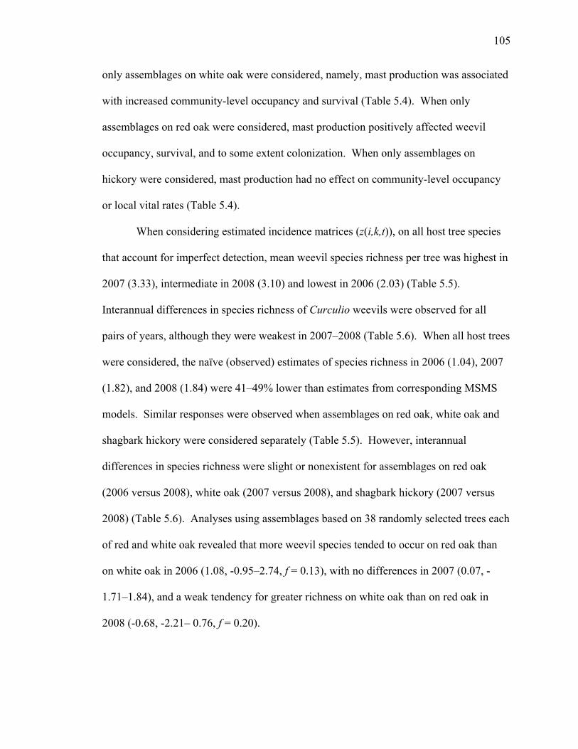
105

only assemblages on white oak were considered, namely, mast production was associated

with increased community-level occupancy and survival (Table 5.4). When only

assemblages on red oak were considered, mast production positively affected weevil

occupancy, survival, and to some extent colonization. When only assemblages on

hickory were considered, mast production had no effect on community-level occupancy

or local vital rates (Table 5.4).

When considering estimated incidence matrices (z(i,k,t)), on all host tree species

that account for imperfect detection, mean weevil species richness per tree was highest in

2007 (3.33), intermediate in 2008 (3.10) and lowest in 2006 (2.03) (Table 5.5).

Interannual differences in species richness of Curculio weevils were observed for all

pairs of years, although they were weakest in 2007–2008 (Table 5.6). When all host trees

were considered, the naïve (observed) estimates of species richness in 2006 (1.04), 2007

(1.82), and 2008 (1.84) were 41–49% lower than estimates from corresponding MSMS

models. Similar responses were observed when assemblages on red oak, white oak and

shagbark hickory were considered separately (Table 5.5). However, interannual

differences in species richness were slight or nonexistent for assemblages on red oak

(2006 versus 2008), white oak (2007 versus 2008), and shagbark hickory (2007 versus

2008) (Table 5.6). Analyses using assemblages based on 38 randomly selected trees each

of red and white oak revealed that more weevil species tended to occur on red oak than

on white oak in 2006 (1.08, -0.95–2.74, f = 0.13), with no differences in 2007 (0.07, -

1.71–1.84), and a weak tendency for greater richness on white oak than on red oak in

2008 (-0.68, -2.21– 0.76, f = 0.20).

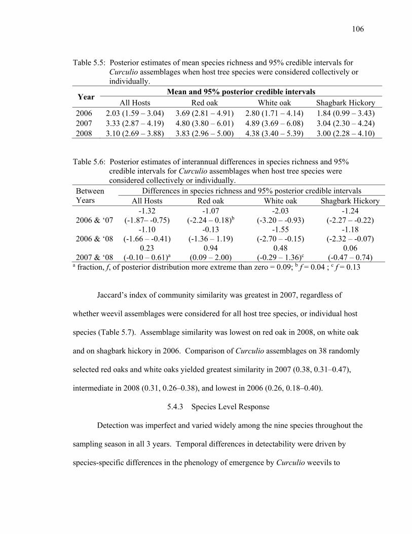
106

Table 5.5: Posterior estimates of mean species richness and 95% credible intervals for

Curculio assemblages when host tree species were considered collectively or individually.

Year Mean and 95% posterior credible intervals All Hosts Red oak White oak Shagbark Hickory

2006 2.03 (1.59 – 3.04) 3.69 (2.81 – 4.91) 2.80 (1.71 – 4.14) 1.84 (0.99 – 3.43) 2007 3.33 (2.87 – 4.19) 4.80 (3.80 – 6.01) 4.89 (3.69 – 6.08) 3.04 (2.30 – 4.24) 2008 3.10 (2.69 – 3.88) 3.83 (2.96 – 5.00) 4.38 (3.40 – 5.39) 3.00 (2.28 – 4.10)

Table 5.6: Posterior estimates of interannual differences in species richness and 95% credible intervals for Curculio assemblages when host tree species were considered collectively or individually.

Between Years

Differences in species richness and 95% posterior credible intervals All Hosts Red oak White oak Shagbark Hickory

2006 & ‘07 -1.32

(-1.87– -0.75) -1.07

(-2.24 – 0.18)b -2.03

(-3.20 – -0.93) -1.24

(-2.27 – -0.22)

2006 & ‘08 -1.10

(-1.66 – -0.41) -0.13

(-1.36 – 1.19) -1.55

(-2.70 – -0.15) -1.18

(-2.32 – -0.07)

2007 & ‘08 0.23

(-0.10 – 0.61)a 0.94

(0.09 – 2.00) 0.48

(-0.29 – 1.36)c 0.06

(-0.47 – 0.74) a fraction, f, of posterior distribution more extreme than zero = 0.09; b f = 0.04 ; c f = 0.13

Jaccard’s index of community similarity was greatest in 2007, regardless of

whether weevil assemblages were considered for all host tree species, or individual host

species (Table 5.7). Assemblage similarity was lowest on red oak in 2008, on white oak

and on shagbark hickory in 2006. Comparison of Curculio assemblages on 38 randomly

selected red oaks and white oaks yielded greatest similarity in 2007 (0.38, 0.31–0.47),

intermediate in 2008 (0.31, 0.26–0.38), and lowest in 2006 (0.26, 0.18–0.40).

5.4.3 Species Level Response

Detection was imperfect and varied widely among the nine species throughout the

sampling season in all 3 years. Temporal differences in detectability were driven by

species-specific differences in the phenology of emergence by Curculio weevils to

107

coincide with seed maturation in their primary host trees. For all species, detection

probability was lowest in early and late season, but peaked during mid season in any year

(Figure 5.2). Similar trends in detection probability were observed for all species in

models comprising only a single tree species.

Table 5.7: Posterior estimates of mean Jaccard similarity and 95% credible intervals for

Curculio assemblages when host tree species were considered collectively or individually.

Year Mean and 95% posterior credible intervals All Hosts Red oak White oak Shagbark Hickory

2006 0.21 (0.16 – 0.38) 0.44 (0.33 – 0.59) 0.30 (0.14 – 0.54) 0.24 (0.11 – 0.49) 2007 0.29 (0.25 – 0.35) 0.45 (0.36 – 0.56) 0.43 (0.33 – 0.56) 0.33 (0.22 – 0.48) 2008 0.27 (0.24 – 0.32) 0.36 (0.29 – 0.47) 0.36 (0.28 – 0.48) 0.34 (0.28 – 0.44)

Mean correlations between occupancy and detection probability were positive

with credible interval coverage of zero. Estimates of detection probability were

improved further by species-specific responses to the covariates Julian date and year.

Using the MSMS model framework with all host trees resulted in more precise estimates

of occupancy (mean reduction in 95% credible interval width of 17.79%), survival rates

(mean reduction of 12.38%), colonization rates (mean reduction of 27.83%), and

covariate effects associated with occupancy, survival and colonization (mean reduction of

41.02%, 4.25% and 45.65% respectively) compared with estimates computed using

single-species models (Figures.5.3 and 5.4, Appendix G, H and J). When all host trees

were considered, mast availability had a positive effect on first-year site occupancy of all

Curculio species, especially so for red-oak specialists (C. nasicus, C. orthorhynchus) and

generalists on red and white oak (C. proboscideus and C.sulcatulus) (Figure 5.3).

109

Figure 5.2: Season and survey-specific estimates of detection probability for acorn

weevils sampled on all three host tree species in west-central Indiana from 2006 (solid line), 2007 (dashed line), and 2008 (dashed dotted line).

Variation in mast production had a greater effect on survival rate than on colonization

rate for all species of weevils (Figure 5.4, Appendix I). For models including data only

from a single host tree species, increased mast production by primary hosts generally

resulted in greater occurrence rates (Appendix J). The effect of mast production on

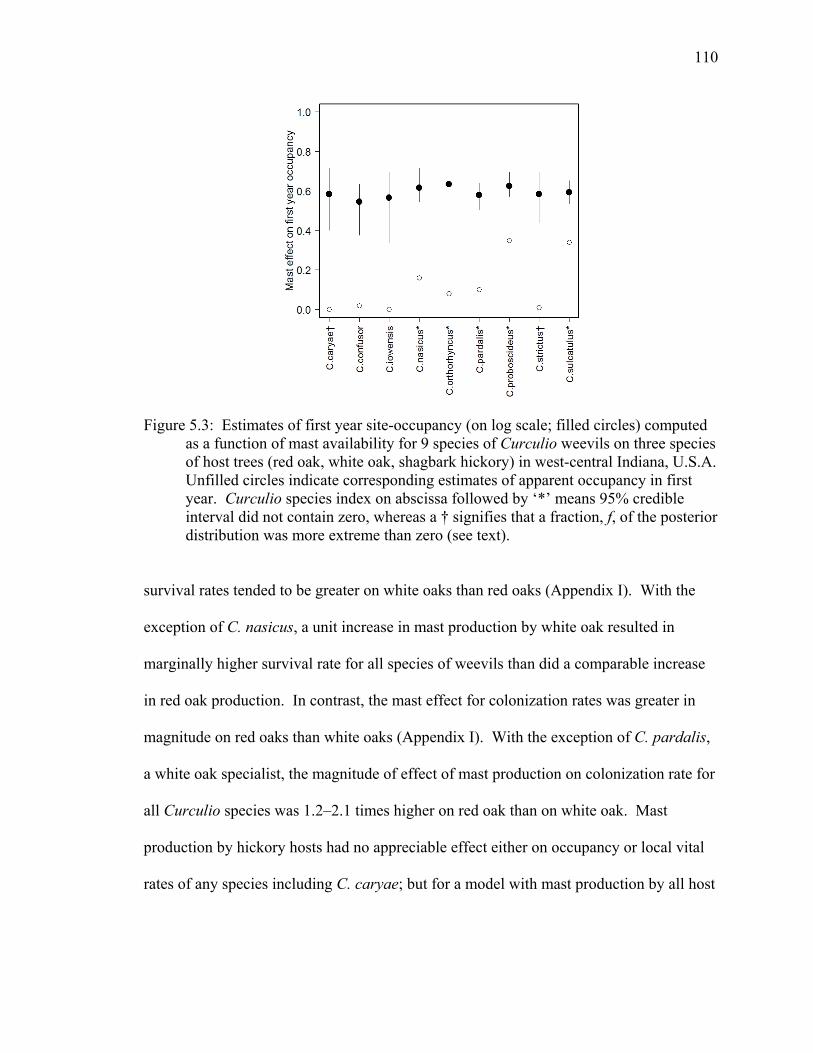
110

Figure 5.3: Estimates of first year site-occupancy (on log scale; filled circles) computed as a function of mast availability for 9 species of Curculio weevils on three species of host trees (red oak, white oak, shagbark hickory) in west-central Indiana, U.S.A. Unfilled circles indicate corresponding estimates of apparent occupancy in first year. Curculio species index on abscissa followed by ‘*’ means 95% credible interval did not contain zero, whereas a † signifies that a fraction, f, of the posterior distribution was more extreme than zero (see text).

survival rates tended to be greater on white oaks than red oaks (Appendix I). With the

exception of C. nasicus, a unit increase in mast production by white oak resulted in

marginally higher survival rate for all species of weevils than did a comparable increase

in red oak production. In contrast, the mast effect for colonization rates was greater in

magnitude on red oaks than white oaks (Appendix I). With the exception of C. pardalis,

a white oak specialist, the magnitude of effect of mast production on colonization rate for

all Curculio species was 1.2–2.1 times higher on red oak than on white oak. Mast

production by hickory hosts had no appreciable effect either on occupancy or local vital

rates of any species including C. caryae; but for a model with mast production by all host

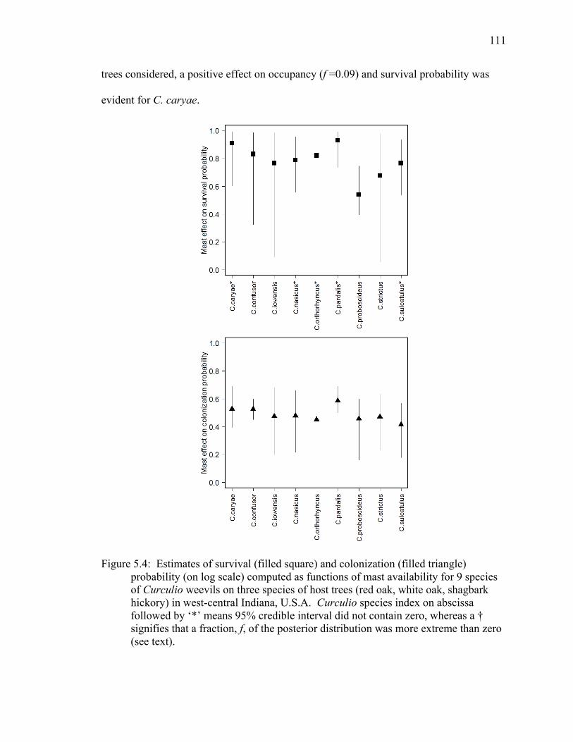
111

trees considered, a positive effect on occupancy (f =0.09) and survival probability was

evident for C. caryae.

Figure 5.4: Estimates of survival (filled square) and colonization (filled triangle) probability (on log scale) computed as functions of mast availability for 9 species of Curculio weevils on three species of host trees (red oak, white oak, shagbark hickory) in west-central Indiana, U.S.A. Curculio species index on abscissa followed by ‘*’ means 95% credible interval did not contain zero, whereas a † signifies that a fraction, f, of the posterior distribution was more extreme than zero (see text).

112

5.5 Discussion

My results provide evidence that weevil assemblages on individual trees are

structured by and responsive to variation in mast production. My predictions related to

the impact of mast production on community-level occupancy dynamics generally were

supported. Mast production was an important predictor of community-level occupancy

and survival rate of acorn weevils (Table 5.4). The community level colonization rate

was also predicted by mast production on red oak. As predicted, the community level

species richness and similarity was highest in 2007, suggesting that coexistence of

species peaked when all of the host tree species experienced mast and the temporal and

spatial availability of resources for consumers were maximized. Weevil species co-

occurred on host trees throughout the study. Spatio-temporal variation in seed production

by oaks and hickories likely facilitated coexistence of weevil species by reducing density-

dependent competition between species. Coexistence was facilitated further by

prolonged diapause (Menu 1993b, Menu and Debouzie 1993), which created a temporal

storage effect, and by differential suitability of hosts as resources for weevil species,

which created a spatial storage effect. Temporal and spatial storage effects associated

with seed banks have been linked to coexistence of desert annual plants competing for

pulsed water availability (Chesson and Warner 1981, Pake and Venable 1995, Chesson

2000, Chesson et al. 2004). Dynamics of acorn weevils likely satisfy the following three

prerequisites for a storage effect to operate and enable coexistence: species (i) experience

buffered population growth due to persistent life history traits (i.e., prolonged diapause),

(ii) differ in their response to the environmental fluctuations in resource availability (see

113

explanation below), and (iii) experience intensified intraspecific competition in a favored

year or patch.

With regard to criterion (i), Curculio are known to exhibit short (3 months) and

prolonged (1 or more years) diapause behavior (Soula and Menu 2005, Mynhardt et al.

2007). For instance, 95% of adults from the same cohort of C. elephas, a European

species, tend to emerge after 1–2 years of diapause (Soula and Menu 2005). In a

community context, prolonged larval diapause ensures that a few adults of almost all

species emerge from soil even under suboptimal conditions and avoid local extinctions in

bad years or at patches of lower resource suitability.

With regard to criterion (ii), species in my Curculio community showed distinct

patterns of host selection and exhibited marked temporal and spatial partitioning of

resource use between and within years. Specifically, occupancy, colonization and

survival probability of C. pardalis, and survival of C. confusor, were positively driven by

mast dynamics on their primary host, white oak. Similarly, occupancy and survival of

red oak specialists, C. nasicus and C. orthorhynchus, were positively influenced by mast

production on their primary host. Mast production of both oak species positively affected

occupancy and/or survival of more generalist species, C. proboscideus and C. sulcatulus.

C. strictus and C. iowensis were too rarely sampled in the study to detect distinct host

selection response; however, marked variation in their detection probabilities likely

reflected seasonal niche partitioning (Figure 5.2). Of the nine species, only C. caryae

failed to show a population response to resource abundance, and I believe this was likely

an artifact due to delayed sampling during 2006 and 2007 that resulted in undersampling

of the species during the period of hickory maturation.

114

With regard to criterion (iii), if a storage effect is operative, an abundant species

in a preferred patch will experience greater intraspecific competition when a host tree

produces a bumper mast crop. In contrast, a rare species with a different preference will

experience less intraspecific competition during a mast year. The predicted result is a

weaker relationship between competition intensity and resource fluctuations for the rarer

species, leading to greater fluctuations in recruitment relative to more abundant species.

In my system, species that were on average rarer also tended to be those with greater

levels of specialization for particular host tree species. I do not have data on recruitment

and hence can only base comparisons on changes in occupancy (and presumably relative

abundance). Consistent with predictions, coefficients of variation in weevil occupancy

across years tended to be higher for the more abundant specialists than for generalists (C.

pardalis [0.91] > C. caryae [0.76] > C. confusor [0.71] > C. nasicus [0.52] > C.

proboscideus [0.11] > C. orthorhynchus [0.10] > C. strictus and C.iowensis [0.08] > C.

sulcatulus [0.04]). The stronger fluctuation in occupancy of the more abundant

specialists is analogous to the storage effect observed for rare versus common tropical

deciduous tree species in Mexico (Kelly and Bowler 2002) and demonstrated

experimentally in arid annual plants with persistent seed banks subjected to varying

availability of water and temperature (Facelli et al. 2005). Because patch suitability need

not be correlated with occupancy or abundance (Van Horne 1983), it may be more

instructive to consider suitability in terms of average fitness based on changes in

occupancy. The per-patch change in occupancy was positive (Ψt -Ψt-1 / Ψt-1 > 0;

Appendix J) and consistent with a storage effect for all but C. nasicus during 2006–07

and 2007–08 and C. pardalis in 2007–08.

115

The generalists C. proboscideus and C. sulcatulus exhibited consistent patterns in

detectability across years, which suggest consistency in temporal dynamics (Figure 5.2).

They also had higher and nearly constant levels of occupancy (Appendix J) even in the

year of red oak mast failure (2008). However, 95% credible intervals indicated that both

species had much higher occupancy (1.03-2.00 times) on red oak relative to white oak in

2006 and 2007 (for C. sulcatulus, 90% credible intervals tended to not overlap in 2007),

suggesting that red oak and white oak hosts may be sources and sinks, respectively, for

these species (Govindan et al. 2012). In the year of red oak mast failure (2008),

colonization rates (2007–08) of C. sulcatulus and C. proboscideus were higher on white

oak than on red oak. Both generalist species thus compensated for their lower survival

rate on white oak than on red oak with higher colonization rates on white during the year

of red oak mast failure. My findings extend earlier work (Govindan et al. 2012), which

showed that survival and colonization of generalists is affected by mast production.

Moreover, increased colonization on a secondary host (white oak) in response to mast

failure on the primary host (red oak) is consistent with source-sink dynamics between red

(source) and white oak (sink) populations of C. sulcatulus and C. proboscideus.

A spatial storage effect was demonstrated for a pair of desert annual plants, with

the competitively inferior Phacelia popeii able to coexist with Erodium cicutarium as a

result of differences in environmental preferences (Sears and Chesson 2007). In my

study, gains made by C. sulcatulus or C. proboscideus in a preferred patch (red oak)

during a favorable mast year were stored temporally and made available in the

subsequent year(s) to local populations occupying a less preferred patch (white oak) in

space. In this context, occupancy dynamics of generalists appear consistent with a spatial

116

and a temporal storage effect operating simultaneously to enable the coexistence of

species in this community. Based on results from single-species occupancy models,

Govindan et al. (2012) predicted that continued loss of white oak (Abrams 2003) likely

poses a greater risk to the most specialized (C. pardalis) of the three species they

considered. My results based on MSMS models concur and extend likely adverse

impacts of white oak loss to all major species of acorn weevils in the guild, but especially

those species that specialize on white oak.

The current study is the first of its kind to assess mechanisms structuring a

community of Curculio weevils in fragmented forest habitats. Previous field surveys of

insect communities (Jeffries et al. 2006), including the one that assessed mechanisms

structuring a Curculio community on two isolated oak trees (Venner et al. 2011), failed to

account for imperfect detection and assumed non-detection as true absence of species

from the site (but see Dorazio et al. 2010, Gotelli et al. 2010). Models ignoring detection

probability lead to biased and less accurate parameter estimates (Gu and Swihart 2004).

Methodologically, I explicitly accounted for imperfect detection to estimate occupancy

for both abundant and rare species using spatially and temporally replicated multi-year

site-occupancy surveys. Naïve occupancy estimates that ignore detection probability

were highly negatively biased for all species and much lower for rare species compared

to estimated occupancies from MSMS models. Estimates of species richness and

similarity indexes from naïve models were also severely underestimated for the most part.

Naïve estimates are especially problematic because rare species dominate local

communities (Gaston 1994), are increasingly vulnerable to anthropogenic disturbances

(Pimm et al. 1998) and are overlooked easily during field sampling, even in highly

117

standardized surveys (Gu and Swihart 2004, Kéry et al. 2009). Importantly, multi-

species modeling integrated data across numerous species and yielded greater precision

and accuracy for parameter estimates associated with rare (as well as common) species

relative to naïve or more conventional single-species approaches. Henceforth, I urge

conservation biologists to use MSMS model as an efficient tool to provide sound

inferences for species conservation and biodiversity protection.

118

CHAPTER 6. CONCLUSION

For the last two decades, ecological research to appreciate the dynamics of

species living in fragmented landscape and the forces that promote coexistence at

community level has focused on the concept of metapopulation dynamics (Hanski 1991,

Hanski and Gilpin 1997, Kun et al. 2009) and its community level (Holt 1997,

Amarasekare 2008) extensions. Here, I briefly present the key results from laboratory

experiments with beetles and field observations on acorn weevils (chapter 2 – 5)

conducted to test theoretical developments in the field of metapopulation ecology. I

discuss the broader implications of the results for species conservation and pest

management, along with potential future directions for theoretical and empirical research.

Chapter 2 and 3 of my dissertation explored the consequences of spatial (Hill and

Caswell 1999, With and King 1999) and temporal (Keymer et al. 2000) dynamics in

availability and suitability of resources for metapopulation dynamics of a well-studied

model organism - the red flour beetle (Tribolium castaneum), in different landscape

settings provisioned in the lab. Specifically, in chapter 2, I investigated the main and

interactive effects of resource availability (constant vs. diminishing), patch connectivity

(low vs. high), and dynamics of patch configuration (static vs. dynamic) on colonization

rate, extinction rate and beetle abundance and metapopulation stability. Most strikingly,

effects of patch connectivity and configuration on dynamics of beetle metapopulations

119

were unexpected, and these effects interacted to influence abundance and stability. High

connectivity increased the colonization rate of beetles into patches and dispersal mortality

of beetles in the matrix, but this effect was less pronounced in dynamic relative to static

landscapes. At constant resource levels, frequency of colonization exceeded extinction in

landscapes with dynamic patches when connectivity was low, and promoted greater patch

occupancy. Constant resources, low connectivity and dynamic patches resulted in

asynchrony in local dynamics, refugia for pupae from cannibalism, and greater adult

abundance. Landscapes with low connectivity and constant resources exhibited strong

negative density dependence of pupae on adults and greatest metapopulation stability.

Metapopulations in control landscapes with no patch connectivity went extinct quickly

and thus had lower persistence than comparable landscapes with low connectivity. The

results suggested the role of intermediate connectivity and patch dynamics for persistence

of species in landscapes not limited by resource availability. The results must be

interpreted with caution, as temporal patch dynamics in four-patch landscapes coincided

with the larval development period and thus reduced the negative consequences for beetle

larvae in habitats.

In chapter 3, I tested the predictions of a spatially and temporally realistic

metapopulation model of DeWoody et al. (2005) using the red flour beetles in

experimental landscapes with the same background destruction rate, but differentiated by

resource structure (homogeneous vs. heterogeneous), patch connectivity (high vs. low)

and patch dynamics (fast vs. slow). Specifically, the effects of the above three factors on

colonization rate, extinction rate, metapopulation capacity and persistence in different

treatment landscapes were assessed and compared. High connectivity increased the

120

colonization rate of beetles, but this effect was less pronounced in heterogeneous relative

to homogeneous landscapes. Higher connectivity and faster patch dynamics increased

extinction rates in landscapes. Lower connectivity promoted density-dependent

emigration. Landscape-level occupancy probability was enhanced in heterogeneous

landscapes with patches of different carrying capacity. Highest metapopulation capacity

and persistence were observed in landscapes with heterogeneous patches, low

connectivity and slow patch dynamics. Metapopulations in control landscapes with no

patch dynamics exhibited rapid declines in abundance and approached extinction due to

higher pupal cannibalism by adults, increased adult mortality in the matrix, and extremely

low dispersal between remaining habitable patches. These results highlighted the role of

intermediate patch dynamics, intermediate connectivity and density dependent emigration

for persistence of species in heterogeneous landscapes.

In Chapter 4, I explored variation in patch (tree-level) occupancy dynamics of

three species of acorn weevils (Curculio) that vary in their specialization, i.e. their

relative selection of red and white oak as hosts: C. pardalis (white oak specialist), C.

sulcatulus (generalist) and C. proboscideus (generalist). Occupancy and vital rates of

weevils on a host tree increased with acorn production and were significantly influenced

by neighborhood forest density. Contrary to prediction, the specialist exhibited greater

occupancy probability in patches than generalists. Closer inspection revealed that red

oak trees occupied by the white oak specialist appeared to function as sink populations

with frequent colonization following local extinction. The specialist weevil species also

exhibited greater relative variation in occupancy and relative abundance on its host trees

among years. As expected, generalists exhibited lower local extinction and colonization

121

rates than the specialist. Across much of their range in the eastern United States acorn

weevils exist in fragmented, temporally dynamic landscapes. My results indicate that

generalists occur on a lower proportion of usable trees but are buffered by access to more

suitable patches and greater patch-specific survival. More generally, my results

demonstrate that estimates of specialization derived from occupancy data may be

misleading in the absence of patch-specific information on vital rates.

Chapter 5 of the dissertation tested whether community structure in acorn weevils

is influenced by spatio-temporal variation in mast availability on host tree species.

Consistent with predictions, mast production had a strong positive effect on community-

level occupancy and patch survival of Curculio weevils. Mean weevil species richness

per tree and community similarity were highest when mast production on all host tree

species was in phase, and lowest when one or most host tree species exhibited mast

failure. Results suggest that coupling of a spatial storage effect with a temporal storage

effect promotes the coexistence of different species of Curculio weevils in fragmented,

temporally dynamic forested landscapes. A spatial storage effect is facilitated by

differential suitability of hosts as resources for weevil species, and a temporal storage

effect is induced by prolonged diapause in Curculio. Both storage effects were more

pronounced for generalist species that evinced source (red oak)–sink (white oak)

dynamics. Coexistence peaked when all of the host tree species produced mast,

maximizing the spatio-temporal availability of resources for consumers.

122

6.1 Broader Implications and Future Directions

Asynchrony in local population dynamics mediated by dispersal between local

populations (Hanski 1999b, Elmhagen and Angerbjorn 2001, Dey and Joshi 2006)

promoted persistence of beetle species in experimental landscapes (Chapter 2) with

temporal patch dynamics and low patch connectivity. Similarly, the dynamics of coupled

subpopulations of beetles in the 12-patch landscapes was influenced by the spatial

arrangement of heterogeneous resource patches. Spatial and temporal heterogeneity in

resource availability facilitated spatial and temporal subsidies and refugia to promote

increased persistence of beetle species (Chapter 3). In a broad sense, temporal patch

dynamics in both experiments mimicked the rotational cropping systems in agro-

ecosystems (Carriere et al. 2012b), where the focus often is on achieving control of

mobile pest species rather than enhancing their persistence. Consistent with my findings,

Carriere and coworkers recently (2012b) investigated the metapopulation dynamics of a

generalist pest species Lygus hesperus (Hemiptera: Miridae) on cotton (Gossypium sps.)

in the San Joaquin Valley in California and showed that spatial patterns in pest density on

cotton can be predicted from variation in surrounding landscape characteristics that

exhibit source – sink characteristics over time. Specifically, groups of cotton fields at a

distance of < 500 m from uncultivated habitats and > 3km from seed alfalfa (Medicago

sativa L.) reduced L. hesperus densities on cotton (Carriere et al. 2012b). Similarly

cotton refugia < 3 km from sampled sites were effective in delaying the evolution of

resistance to the insecticide pyriproxyfen in Bemisia tabaci on cotton (Carriere et al.

2012a). Their findings suggest that a spatially explicit approach accounting for source –

sink characteristics of landscapes coupled with demography and dispersal dynamics of

123

pests can provide strong insights for landscape-level integrated pest management

strategies for such polyphagous pests.

Experiments in landscapes with 12 patches (Chapter 3) with low patch

connectivity evinced density-dependent emigration of beetles, which along with

intermediate patch dynamics resulted in intermediate dispersal rates, lower demographic

stochasticity, and higher species persistence. Density-dependent emigration implies a

direct effect of local population dynamics on the regional (extinction – colonization)

process (Hauzy et al. 2010). Not surprisingly, the results demonstrated the importance of

incorporating local dynamics into estimation of metapopulation capacity (Akcakaya et al.

2004). The results also warrant detailed theoretical and empirical investigation on the

role of dispersal on metapopulation dynamics to appreciate its implications for pest

management in agro-ecosystems (Holt 1997, Carriere et al. 2012b) and species

conservation in fragmented landscapes (Hodgson et al. 2009, Kun et al. 2009).

Accurate estimation of dispersal rates between subpopulations is important to

better understand metapopulation dynamics. Estimation of dispersal rates for beetles in

12-patch landscapes was based on local variance-covariance structure in coupled

subpopulations and relied on the assumption of temporally non varying connectivity

between patches. However, 12-patch landscapes experienced temporal dynamics of

patch creation and destruction, and thus violated this assumption. Further work is needed

to improve estimation of dispersal rate by accounting for a temporally varying

connectivity matrix or by selection of a connectivity matrix that suits the data most using

a maximum likelihood approach (Schneeberger and Jansen 2006). Additionally, I altered

patch connectivity by manipulating the difficulty with which emigration occurred.

124

Recent work by Romero et al. (2010) showed that search behavior in red flour beetles

determines its ability to find patches and follows a simple distance-decay function. Only

63% and 43% of their adult beetles occupied destination patches (with and without flour

combined), when released at distances of 2 - 4 cm and 8 cm respectively; the proportions

declined to 45% (with flour) and 27% (without flour), respectively, at a destination

distance of 16 cm from the source patch. Of the 66 combinations of inter-patch distances

in our12-patch landscape, 38% were > 8cm and 58% were > 16cm, likely explaining the

high dispersal mortality experienced in the matrix in my landscape. Recent

investigations on the behavioral differences in dispersers and patch residents have

characterized them based on a suite of distinct personality-dependent phenotypic traits

and demand theoretical investigations into the consequences of these traits for re-

introduction strategies (Cote et al. 2010). Dispersers can also have different phenotypic

traits that distinguish them based on their ability to colonize extinct patches and rescue

already extant patches in a metapopulation (Cote et al. 2010).

Investigations on the metapopulation and metacommunity dynamics of Curculio

weevils involved estimation of the occupancy, extinction and colonization rates on their

host trees as well as community levels attributes like species richness and similarity.

Despite repeated surveys, the observed ‘absences’ of species in their patches may often

be overlooked ‘presences’ (Gu and Swihart 2004), and so I explicitly accounted for

detection probability to reduce bias in parameter estimation. However, like seed banks in

plants (Freckleton and Watkinson 2002), Curculio weevils exhibit prolonged larval

diapause behavior (Menu and Debouzie 1993). Mature larvae leave the infested acorns

and overwinter in the soil underneath the host tree. In European chestnut weevil,

125

Curculio elephas, larvae burrow into soil to an average depth of 8.4 0.2 ( SE) cm

(Menu and Desouhant 2002); diapause begins in October and terminates in December but

with slow developmental rates and later morphogenesis proceeds rapidly from March

until adult emergence (Menu 1993b, Menu and Debouzie 1993). Evidence from field

experiments with C. elephas suggests average adult emergence rate of 14% ( 5) over 3

years (Menu and Desouhant 2002). Of the emerged adults, 59% ( 3), 37% ( 3) and 4%

( 1) emerged after 1, 2 and 3 years of overwintering. Similar information is lacking on

acorn weevils of North America and warrants detailed studies on the prolonged diapause

behavior and mechanisms that regulate diapause (Higaki 2005, Soula and Menu 2005,

Higaki and Toyama 2011) to appreciate the biology and dynamics of these species and

factors structuring these communities.

Prolonged larval diapause in acorn weevils makes it difficult to detect the cryptic

life stages, which may remain undetected in their local patches for one or more years

even after making regular repeated visits within each year. Non-detection of adults in

several repeated visits made across multiple years, and an inability to observe a cryptic

life stage can lead to false extinctions at the local host tree level. Patch occupancy

models based on these detection – non detection data would estimate the extinction rates

at the local host tree level with high certainty and skew the estimation of extinction and

colonization rates upward, detection probability downward and estimated occupancy

probability would be highly variable (Lamy et al. 2013). A recent multistate occupancy

model for a tropical freshwater snail Drepanotrema depressissimum, with cryptic life

stages handled this bias in estimation of colonization and extinction rates for the patches

by conditioning it on a specific, unambiguously observable state of the patch, which was

126

associated with the cryptic life stage (Lamy et al. 2013). For instance, the occupancy

dynamics of the snail was modeled by assuming that resistant (cryptic) and normal forms

are associated with two different habitats with specific environmental characteristics,

namely dry and wet sites, respectively. Identification of comparable habitat or

environmental characteristics to unambiguously model the presence of larvae in

prolonged diapause is needed to estimate more reliable turnover rates for acorn weevils

on their host trees. The estimation of transition probabilities among three occupancy

states (say, unoccupied, occupied by Curculio larvae in prolonged diapause, and occupied

by adult Curculio weevils) can be implemented using dynamic multistate occupancy

modeling (Mackenzie et al. 2009).

Occupancy modeling on acorn weevils also assumed that the population is closed

between surveys within a year (season), and that extinctions and recolonizations in

patches are possible only between years. However, my findings suggest that acorn

weevils exhibit source (red oak)–sink (white oak) dynamics on their habitat patches, and

a spatial and temporal storage effect is potentially acting together to favor coexistence of

species in this community (Chesson et al. 2004). What this suggests is that even the true

extinction events in patches can be easily overlooked in surveys when re-colonization

occurs from neighboring patches between the surveys (Lamy et al. 2012). Such a

violation of assumptions might lead to estimates of increased detection probability,

increased occupancy, and decreased extinction rate for species in their patches. The bias

in estimated rates of occupancy and vital rates can be independently validated with

genetic data to distinguish true extinctions from apparent extinction (Lamy et al. 2012).

Temporal genetic analysis that explore changes in allelic frequencies should enable

127

differentiation of the different genetic signatures left in the population recolonized by

immigrants from neighboring patches and in the population reconstituted from

individuals in the local patch after an apparent extinction. I agree with Lamy et al. (2012)

that future metapopulation studies should integrate demographic and ecological

observations with genetic studies and vice-versa to gain better insight into

metapopulation dynamics.

The metapopulation concept is well suited to address the dynamics of single-

species, but it ignores species interactions. Not surprisingly, the seminal paper on

metapopulation dynamics (Levins 1969) ignored the presence of natural enemies in agro-

ecosystems and concluded that synchrony in control measures would greatly reduce the

metapopulation densities of pests. However, deterministic metapopulation models by

Ives and Settle (1997) demonstrated that the outcome of synchronous versus

asynchronous planting of crops for pest control depends on the presence / absence of

natural enemies, as their survival is at stake if the prey density declines beyond a

threshold value. Specifically, they showed that pest densities are reduced with

synchronous planting in the absence of predators, and may decrease with asynchronous

planting in the presence of predators depending on the population dynamics and dispersal

abilities of both prey and predators. Insect pests with relatively high dispersal ability and

predators with alternate prey species may be able to out-compete each other and alter the

outcome in favor of or against the pest species, respectively.

My investigations on the effect of mast on acorn weevil assemblages dealt with a

metacommunity (i.e., a multispecies metapopulation) of nine species of weevils but also

ignored interactions between species. Indeed, the effect of landscape fragmentation on

128

biodiversity is dependent on the degree of interactions among species within the

communities (metacommunities), how these interactions are modified by the spatial

dynamics of individual metapopulations and vice versa (Hanski and Gilpin 1997, Holt

1997, Holyoak et al. 2005), and how such pairwise interactions are embedded in more

complex multispecies communities to form the food webs (Amarasekare 2008). Future

studies should consider exploring the dynamics of a Curculio weevil community (or flour

beetle communities in experimental landscapes) that explicitly consider interactions in an

environment with temporally and spatially fluctuating resources or containing more

complex food web interactions, the factors influencing the strength of trophic interactions,

and their stability (Amarasekare 2008).

As in the case of metapopulations, effects of habitat fragmentation on long-term

persistence and stability of interacting metapopulations (i.e., a metacommunity) have also

received special attention (Holyoak and Lawler 1996a, b, Janssen et al. 1997, Swihart et

al. 2001). Recent modeling efforts on predator – prey metacommunity dynamics have

shown the importance of density-dependent dispersal and relative dispersal ability of

species in understanding the response of ecosystems to fragmentation (Hauzy et al. 2010).

Intraspecific density-dependent dispersal may synchronize or desynchronize the local

dynamics depending on dispersal rates of prey and predator. In contrast, interspecific

density-dependent dispersal always leads to asynchrony in local dynamics. Both types of

dispersal also have been shown to enhance the top-down control of the prey by the

predator, resulting in increased regional stability of the metacommunity at intermediate

dispersal rates. Additional modeling efforts with more patches of different carrying

capacity (spatial heterogeneity; Garvie and Golinski 2010), varied levels of patch

129

connectivity (Hodgson et al. 2009) or migratory corridor effects (Garvie and Golinski

2010) and stochastic patch creation and destruction rates are needed to better appreciate

the ramifications of spatio-temporal resource availability (Ives and Settle 1997,

Amarasekare 2008) for relative dispersal ability of predators and prey (Hauzy et al. 2010)

and for their metacommunity dynamics. Amarasekare (2008) also emphasizes the need

for comparative analysis of different types of spatial mechanisms (spatial coupling, and

metacommunity dynamics [extinction-colonization, and emigration-immigration]), across

a given food web module (intraguild predation/omnivory, predation) with or without

local niche partitioning (apparent competition, exploitative competition), as well as of a

given spatial mechanism across different types of food web modules. Empirical support

for theoretical predictions on predator-prey or host-parasitoid (but see Holyoak and

Lawler 1996b, Bonsall and Hassell 1998, Bull et al. 2006) metapopulation dynamics

(Garvie and Golinski 2010), and food web dynamics (Amarasekare 2008) are scarce and

clearly warrant more field and laboratory experiments to increase our ability to predict

the effects of habitat fragmentation on the stability of ecosystems (Hauzy et al. 2010).

130

LITERATURE CITED

130

LITERATURE CITED

Abrams, M. D. 1992. Fire and the development of oak forests - in eastern North-America, oak distribution reflects a variety of ecological paths and disturbance conditions. Bioscience 42:346-353.

Abrams, M. D. 1998. The red maple paradox. Bioscience 48:355-364.

Abrams, M. D. 2003. Where has all the white oak gone? Bioscience 53:927-939.

Akcakaya, H. R., V. C. Radeloff, D. J. Mlandenoff, and H. S. He. 2004. Integrating landscape and metapopulation modeling approaches: Viability of the sharp-tailed grouse in a dynamic landscape. Conservation Biology 18:526-537.

Aldrich, P. R., G. R. Parker, J. S. Ward, and C. H. Michler. 2003. Spatial dispersion of trees in an old-growth temperate hardwood forest over 60 years of succession. Forest Ecology and Management 180:475-491.

Amarasekare, P. 2008. Spatial Dynamics of Foodwebs. Annual Review of Ecology Evolution and Systematics 39:479-500.

Bancroft, J. S. 2001. Intraspecific interaction and mechanisms of population regulation in experimentally limited habitat. Environmental Entomology 30:1061-1072.

Bancroft, J. S. and P. Turchin. 2003. An experimental test of fragmentation and loss of habitat with Oryzaephilus surinamensis. Ecology 84:1756-1767.

Bartoń, K. 2013. MuMIn: Multi-model inference (R package version 1.9.5).

Bascompte, J. 2001. Aggregate statistical measures and metapopulation dynamics. Journal of Theoretical Biology 209:373-379.

131

Bascompte, J. and R. V. Sole1996 .׳. Habitat fragmentation and extinction thresholds in spatially explicit models. Journal of Animal Ecology 65:465-473.

Bengtsson, J. 1989. Interspecific competition increases local extinction rate in a metapopulation system. Nature 340:713-715.

Bengtsson, J. and G. Milbrink. 1995. Predicting extinctions : interspecific competition, predation and population variability in experimental Daphnia populations. Oecologia 101:397-406.

Benoit, H. P., E. McCauley, and J. R. Post. 1998. Testing the demographic consequences of cannibalism in Tribolium confusum. Ecology 79:2839-2851.

Bergman, K. O. and O. Kindvall. 2004. Population viability analysis of the butterfly Lopinga achine in a changing landscape in Sweden. Ecography 27:49-58.

Biedermann, R. 2004. Modelling the spatial dynamics and persistence of the leaf beetle Gonioctena olivacea in dynamic habitats. Oikos 107:645-653.

Bonsall, M. B. and M. P. Hassell. 1998. Population dynamics of apparent competition in a host-parasitoid assemblage. Journal of Animal Ecology 67:918-929.

Boudjemadi, K., J. Lecomte, and J. Clobert. 1999. Influence of connectivity on demography and dispersal in two contrasting habitats: an experimental approach. Journal of Animal Ecology 68:1207-1224.

Bretz, F., T. Hothorn, and P. Westfall. 2010. Multiple Comparisons Using R. CRC Press, Boca Raton.

Brooks, S. P. and A. Gelman. 1998. General methods for monitoring convergence of iterative simulations. Journal of Computational and Graphical Statistics 7:434-455.

Bull, J. C., N. J. Pickup, M. P. Hassell, and M. B. Bonsall. 2006. Habitat shape, metapopulation processes and the dynamics of multispecies predator-prey interactions. Journal of Animal Ecology 75:899-907.

132

Bullock, J. M., I. L. Moy, R. F. Pywell, S. J. Coulson, A. M. Nolan, and H. Caswell. 2002. Plant dispersal and colonization processes at local and landscape scales. Pages 279-302 in J. M. Bullock, R. Kenward, and R. Hails, editors. Dispersal Ecology. Blackwell Science, Oxford.

Burnham, K. P. and D. A. Anderson. 2002. Model selection and multimodel inference: a practical information-theoretic approach. 2nd edition. Springer-Verlag, New York, USA.

Campbell, J. F. and C. Runnion. 2003. Patch exploitation by female red flour beetles, Tribolium castaneum. Journal of Insect Science 3:20.

Carriere, Y., C. Ellers-Kirk, K. Hartfield, G. Larocque, B. Degain, P. Dutilleul, T. J. Dennehy, S. E. Marsh, D. W. Crowder, X. C. Li, P. C. Ellsworth, S. E. Naranjo, J. C. Palumbo, A. Fournier, L. Antilla, and B. E. Tabashnik. 2012a. Large-scale, spatially-explicit test of the refuge strategy for delaying insecticide resistance. Proceedings of the National Academy of Sciences of the United States of America 109:775-780.

Carriere, Y., P. B. Goodell, C. Ellers-Kirk, G. Larocque, P. Dutilleul, S. E. Naranjo, and P. C. Ellsworth. 2012b. Effects of Local and Landscape Factors on Population Dynamics of a Cotton Pest. Plos One 7.

Chesson, P. 2000. Mechanisms of maintenance of species diversity. Annual Review of Ecology and Systematics 31:343-366.

Chesson, P., R. L. E. Gebauer, S. Schwinning, N. Huntly, K. Wiegand, M. S. K. Ernest, A. Sher, A. Novoplansky, and J. F. Weltzin. 2004. Resource pulses, species interactions, and diversity maintenance in arid and semi-arid environments. Oecologia 141:236-253.

Chesson, P. L. and R. R. Warner. 1981. Environmental variability promotes coexistence in lottery competitive-systems. American Naturalist 117:923-943.

Cook, W. M. and R. D. Holt. 2006. Influence of multiple factors on insect colonization of heterogeneous landscapes: A review and case study with periodical cicadas (Homoptera : Cicadidae). Annals of the Entomological Society of America 99:809-820.

133

Cote, J., J. Clobert, T. Brodin, S. Fogarty, and A. Sih. 2010. Personality-dependent dispersal: characterization, ontogeny and consequences for spatially structured populations. Philosophical Transactions of the Royal Society B-Biological Sciences 365:4065-4076.

Cottrell, T. E. and B. W. Wood. 2008. Movement of adult pecan weevils Curculio caryae within pecan orchards. Agricultural and Forest Entomology 10:363-373.

Crawley, M. J. and C. R. Long. 1995. Alternate bearing, predator satiation and seedling recruitment in Querrcus robur L. Journal of Ecology 83:683-696.

Debinski, D. M. and R. D. Holt. 2000. A survey and overview of habitat fragmentation experiments. Conservation Biology 14:342-355.

Desharnais, R. A. and L. Liu. 1987. Stable demographic limit cycles in laboratory populations of Tribolium castaneum. Journal of Animal Ecology 56:885-906.

Devictor, V., J. Clavel, R. Julliard, S. Lavergne, D. Mouillot, W. Thuiller, P. Venail, S. Villeger, and N. Mouquet. 2010. Defining and measuring ecological specialization. Journal of Applied Ecology 47:15-25.

Devictor, V., R. Julliard, J. Clavel, F. Jiguet, A. Lee, and D. Couvet. 2008a. Functional biotic homogenization of bird communities in disturbed landscapes. Global Ecology and Biogeography 17:252-261.

Devictor, V., R. Julliard, and F. Jiguet. 2008b. Distribution of specialist and generalist species along spatial gradients of habitat disturbance and fragmentation. Oikos 117:507-514.

DeWoody, Y. D., Z. L. Feng, and R. K. Swihart. 2005. Merging spatial and temporal structure within a metapopulation model. American Naturalist 166:42-55.

Dey, S. and A. Joshi. 2006. Stability via asynchrony in Drosophila metapopulations with low migration rates. Science 312:434-436.

Dixon, M. D., W. C. Johnson, and C. S. Adkisson. 1997. Effects of weevil larvae on acorn use by blue jays. Oecologia 111:201-208.

134

Dorazio, R. M., M. Kery, J. A. Royle, and M. Plattner. 2010. Models for inference in dynamic metacommunity systems. Ecology 91:2466-2475.

Dorazio, R. M. and J. A. Royle. 2005. Estimating size and composition of biological communities by modeling the occurrence of species. Journal of the American Statistical Association 100:389-398.

Dorazio, R. M., J. A. Royle, B. Soderstrom, and A. Glimskar. 2006. Estimating species richness and accumulation by modeling species occurrence and detectability. Ecology 87:842-854.

Downie, N. M. and J. Arnett, R. H. 1996. The beetles of northeastern North America. Volumes I & II. The Sandhill Crane Press, Gainesville.

Drechsler, M. and C. Wissel. 1998. Trade-offs between local and regional scale management of metapopulations. Biological Conservation 83:31-41.

Eichel, S. and T. Fartmann. 2008. Management of calcareous grasslands for Nickerl's fritillary (Melitaea aurelia) has to consider habitat requirements of the immature stages, isolation, and patch area. Journal of Insect Conservation 12:677-688.

Ellison, A. M., M. S. Bank, B. D. Clinton, E. A. Colburn, K. Elliott, C. R. Ford, D. R. Foster, B. D. Kloeppel, J. D. Knoepp, G. M. Lovett, J. Mohan, D. A. Orwig, N. L. Rodenhouse, W. V. Sobczak, K. A. Stinson, J. K. Stone, C. M. Swan, J. Thompson, B. Von Holle, and J. R. Webster. 2005. Loss of foundation species: consequences for the structure and dynamics of forested ecosystems. Frontiers in Ecology and the Environment 3:479-486.

Elmhagen, B. and A. Angerbjorn. 2001. The applicability of metapopulation theory to large mammals. Oikos 94:89-100.

Espelta, J. M., R. Bonal, and B. Sanchez-Humanes. 2009. Pre-dispersal acorn predation in mixed oak forests: interspecific differences are driven by the interplay among seed phenology, seed size and predator size. Journal of Ecology 97:1416-1423.

ESRI. 2006. ArcGIS 9.2. ESRI (Environmental Systems Research Institute), Redlands, California, USA.

135

Facelli, J. M., P. Chesson, and N. Barnes. 2005. Differences in seed biology of annual plants in arid lands: A key ingredient of the storage effect. Ecology 86:2998-3006.

Fahrig, L. 2002. Effect of habitat fragmentation on the extinction threshold: A synthesis. Ecological Applications 12:346-353.

Forney, K. A. and M. E. Gilpin. 1989. Spatial structure and population extinction - a study with Drosophila flies. Conservation Biology 3:45-51.

Frank, K. and C. Wissel. 1998. Spatial aspects of metapopulation survival - from model results to rules of thumb for landscape management. Landscape Ecology 13:363-379.

Franklin, A. B., B. R. Noon, and T. L. George. 2002. What is habitat fragmentation? Effects of Habitat Fragmentation on Birds in Western Landscapes: Contrasts with Paradigms from the Eastern United States:20-29.

Freckleton, R. P. and A. R. Watkinson. 2002. Large-scale spatial dynamics of plants: metapopulations, regional ensembles and patchy populations. Journal of Ecology 90:419-434.

Fronhofer, E. A., A. Kubisch, F. M. Hilker, T. Hovestadt, and H. J. Poethke. 2012. Why are metapopulations so rare? Ecology 93:1967-1978.

Galford, J. R., J. W. Peacock, and S. L. Wright. 1998. Insects and other pests affecting oak regeneration. Pages 219-225 in H. C. Smith, A. W. Perkey, and W. E. Jr. Kidd, editors. Guidelines for regenerating Appalachian hardwood stands: workshop proceedings. 1998 May 24-26. Morgantown, WV. SAF Publ. 88-03. Morgantown, WV: West Virginia University Books.

Garvie, M. R. and M. Golinski. 2010. Metapopulation dynamics for spatially extended predator-prey interactions. Ecological Complexity 7:55-59.

Gaston, K. J. 1994. Rarity. Chapman & Hall, London.

Gelman, A. and J. Hill. 2007. Data analysis using regression and multilevel/hierarchical models. Cambridge University Press, Cambridge, UK.

136

Gelman, A., X. L. Meng, and H. Stern. 1996. Posterior predictive assessment of model fitness via realized discrepancies. Statistica Sinica 6:733-760.

Gibson, L. P. 1964. Biology and life history of acorn-infesting weevils of the genus Conotrachelus (Coleoptera: Curculionidae). Annals of the Entomological Society of America 57:521-526.

Gibson, L. P. 1969. Monograph of the genus Curculio in the New World (Coleoptera: Curculionidae) USA and Canada. Miscellaneous Publications of the Entomological Society of America 6:241-285.

Gibson, L. P. 1972. Insects that damage white oak acorns. U S Forest Service Research Paper NE:1-7.

Gilpin, M. and I. Hanski. 1991. Metapopulation Dynamics: Empirical and Theoretical Investigations. Academic Press, London.

Godoy, W. A. C. and M. I. S. Costa. 2005. Dynamics of extinction in coupled populations of the flour beetle Tribolium castaneum. Brazilian Journal of Biology 65:271-280.

Gotelli, N. J., R. M. Dorazio, A. M. Ellison, and G. D. Grossman. 2010. Detecting temporal trends in species assemblages with bootstrapping procedures and hierarchical models Philosophical Transactions of the Royal Society. Biological Sciences 365:3621-3631.

Govindan, B. N., M. Kéry, and R. K. Swihart. 2012. Host selection and responses to forest fragmentation in acorn weevils: Inferences from hierarchical dynamic occupancy models. Oikos 121:623 – 633.

Govindan, B. N. and R. K. Swihart. 2012. Experimental Beetle Metapopulations Respond Positively to Dynamic Landscapes and Reduced Connectivity. Plos One 7(4):e34518.

Gribko, L. S. 1995. The effect of acorn insects on the establishment and vigor of northern red oak seedlings in north-central West Virginia. U. S. Department of Agriculture, Forest Service, General Technical Report NE-197, Morgantown, WV.

137

Gu, W. D. and R. K. Swihart. 2004. Absent or undetected? Effects of non-detection of species occurrence on wildlife-habitat models. Biological Conservation 116:195-203.

Gyllenberg, M. and I. Hanski. 1997. Habitat deterioration, habitat destruction, and metapopulation persistence in a heterogenous landscape. Theoretical Population Biology 52:198-215.

Haas, J. P. and E. J. Heske. 2005. Experimental study of the effects of mammalian acorn predators on red oak acorn survival and germination. Journal of Mammalogy 86:1015-1021.

Hanski, I. 1989. Metapopulation Dynamics - Does It Help to Have More of the Same. Trends in Ecology & Evolution 4:113-114.

Hanski, I. 1991. Single-species metapopulation dynamics - concepts, models and observations. Biological Journal of the Linnean Society 42:17-38.

Hanski, I. 1994. A practical model of metapopulation dynamics. Journal of Animal Ecology 63:151-162.

Hanski, I. 1996. Metapopulation ecology. Population dynamics in ecological space and time:13-43.

Hanski, I. 1998. Metapopulation dynamics. Nature 396:41-49.

Hanski, I. 1999a. Habitat connectivity, habitat continuity, and metapopulations in dynamic landscapes. Oikos 87:209-219.

Hanski, I. 1999b. Metapopulation ecology. Oxford University Press, Oxford, UK.

Hanski, I. and M. Gilpin, E. 1997. Metapopulation biology: ecology, genetics, and evolution. Academic Press, San Diego.

Hanski, I. and M. Gyllenberg. 1993. Two general metapopulation models and the core-satellite species hypothesis. American Naturalist 142:17-41.

138

Hanski, I. and O. Ovaskainen. 2000. The metapopulation capacity of a fragmented landscape. Nature 404:755-758.

Hanski, I., T. Pakkala, M. Kuussaari, and G. C. Lei. 1995. Metapopulation Persistence of an Endangered Butterfly in a Fragmented Landscape. Oikos 72:21-28.

Harding, K. and J. M. McNamara. 2002. A unifying framework for metapopulation dynamics. American Naturalist 161:168-168.

Harrison, S. and E. Bruna. 1999. Habitat fragmentation and large-scale conservation: what do we know for sure? Ecography 22:225-232.

Hastings, A. and S. Harrison. 1994. Metapopulation dynamics and genetics. Annual Review of Ecology and Systematics 25:167-188.

Hauzy, C., M. Gauduchon, F. D. Hulot, and M. Loreau. 2010. Density-dependent dispersal and relative dispersal affect the stability of predator-prey metacommunities. Journal of Theoretical Biology 266:458-469.

Hess, G. R. 1996. Linking extinction to connectivity and habitat destruction in metapopulation models. American Naturalist 148:226-236.

Higaki, M. 2005. Effect of temperature on, the termination of prolonged larval diapause in the chestnut weevil Curculio sikkimensis (Coleoptera : Curculionidae). Journal of Insect Physiology 51:1352-1358.

Higaki, M. and M. Toyama. 2011. Evidence for reversible change in intensity of prolonged diapause in the chestnut weevil Curculio sikkimensis. Journal of Insect Physiology.

Hill, M. F. and H. Caswell. 1999. Habitat fragmentation and extinction thresholds on fractal landscapes. Ecology Letters 2:121-127.

Hodgson, J. A., A. Moilanen, and C. D. Thomas. 2009. Metapopulation responses to patch connectivity and quality are masked by successional habitat dynamics. Ecology 90:1608-1619.

139

Holt, R. D. 1997. From metapopulation dynamics to community structure: some consequences of spatial heterogeneity. Pages 149–164 in I. Hanski and M. E. Gilpin, editors. Metapopulation Dynamics: Ecology, Genetics and Evolution. Academic, New York.

Holyoak, M. and S. P. Lawler. 1996a. Persistence of an extinction-prone predator-prey interaction through metapopulation dynamics. Ecology 77:1867-1879.

Holyoak, M. and S. P. Lawler. 1996b. The role of dispersal in predator-prey metapopulation dynamics. Journal of Animal Ecology 65:640-652.

Holyoak, M., A. Leibold M, and R. D. Holt, editors. 2005. Metacommunities: Spatial Dynamics and Ecological Communities. University of Chicago Press, Chicago.

Hovestadt, T. and H. J. Poethke. 2006. The control of emigration and its consequences for the survival of populations. Ecological Modelling 190:443-453.

Ives, A. R. and W. H. Settle. 1997. Metapopulation dynamics and pest control in agricultural systems. American Naturalist 149:220-246.

Janssen, A., E. vanGool, R. Lingeman, J. Jacas, and G. vandeKlashorst. 1997. Metapopulation dynamics of a persisting predator-prey system in the laboratory: time series analysis. Experimental & Applied Acarology 21:415-430.

Jeffries, J. M., R. J. Marquis, and R. E. Forkner. 2006. Forest age influences oak insect herbivore community structure, richness, and density. Ecological Applications 16:901-912.

Johnson, W. C., C. S. Adkisson, T. R. Crow, and M. D. Dixon. 1997. Nut caching by blue jays (Cyanocitta cristata L.): Implications for tree demography. American Midland Naturalist 138:357-370.

Jones, C. G., R. S. Ostfeld, M. P. Richard, E. M. Schauber, and J. O. Wolff. 1998. Chain reactions linking acorns to gypsy moth outbreaks and Lyme disease risk. Science 279:1023-1026.

Julliard, R., J. Clavel, V. Devictor, F. Jiguet, and D. Couvet. 2006. Spatial segregation of specialists and generalists in bird communities. Ecology Letters 9:1237-1244.

140

Kellner, K. F., J. K. Riegel, N. I. Lichti, and R. K. Swihart. 2012. Oak mast production and animal impacts on acorn survival in the Central Hardwoods.

Kellner, K. F., J. K. Riegel, N. I. Lichti, and R. K. Swihart. In Press. Oak mast production and animal impacts on acorn survival in the Central Hardwoods.in R. K. Swihart, M. R. Saunders, R. A. Kalb, S. Haulton, and C. H. Michler, editors. U. S. Department of Agriculture, Forest Service, General Technical Report NE-xxx.

Kelly, C. K. and M. G. Bowler. 2002. Coexistence and relative abundance in forest trees. Nature 417:437-440.

Kelly, D. 1994. The evolutionary ecology of mast seeding. Trends in Ecology & Evolution 9:465-470.

Kelly, D. and V. L. Sork. 2002. Mast seeding in perennial plants: Why, how, where? Annual Review of Ecology and Systematics 33:427-447.

Kéry, M. 2010. Introduction to WinBUGS for Ecologists: A Bayesian approach to regression, ANOVA, mixed models and related analyses. Academic Press, Burlington, MA, USA.

Kéry, M., J. A. Royle, M. Plattner, and R. M. Dorazio. 2009. Species richness and occupancy estimation in communities subject to temporary emigration. Ecology 90:1279-1290.

Kéry, M. and M. Schaub. 2011. Bayesian Population Analysis Using WinBUGS – A Hierarchical Perspective. Academic Press, Waltham, Massachussets, USA.

Keymer, J. E., P. A. Marquet, J. X. Velasco-Hernandez, and S. A. Levin. 2000. Extinction thresholds and metapopulation persistence in dynamic landscapes. American Naturalist 156:478-494.

Kindvall, O. 1999. Dispersal in a metapopulation of the bush cricket, Metrioptera bicolor (Orthoptera : Tettigoniidae). Journal of Animal Ecology 68:172-185.

141

Kirkpatrick, R. L. and P. J. Pekins. 2002. Nutritional value of acorns for wildlife. Pages 173-181 in W. J. McShea and W. M. Healy, editors. Oak forest ecosystems: ecology and management for wildlife. The Johns Hopkins University Press, Baltimore, MD.

Koelle, K. and J. Vandermeer. 2005. Dispersal-induced desynchronization: from metapopulations to metacommunities. Ecology Letters 8:167-175.

Koenig, W. D. and J. M. H. Knops. 2002. The behavioral ecology of masting in oaks. Pages 129-148 in W. J. McShea and W. M. Healy, editors. Oak forest ecosystems. The Johns Hopkins University Press, Baltimore,MD.

Kun, A., B. Oborny, and U. Dieckmann. 2009. Intermediate landscape disturbance maximizes metapopulation density. Landscape Ecology 24:1341-1350.

Lamy, T., O. Gimenez, J. P. Pointier, P. Jarne, and P. David. 2013. Metapopulation Dynamics of Species with Cryptic Life Stages. American Naturalist 181:479-491.

Lamy, T., J. P. Pointier, P. Jarne, and P. David. 2012. Testing metapopulation dynamics using genetic, demographic and ecological data. Molecular Ecology 21:1394-1410.

Lavie, B. and U. Ritte. 1978. Relation between dispersal behavior and reproductive fitness in the flour beetle Tribolium Castaneum. Canadian Journal of Genetics and Cytology 20:589-595.

Leelaja, B. C., Y. Rajashekar, and S. Rajendran. 2007. Detection of eggs of stored-product insects in flour with staining techniques. Journal of Stored Products Research 43:206-210.

Legendre, P. and L. Legendre. 1998. Numerical ecology. Second edition. Elsevier, Amsterdam, The Netherlands.

Levin, S. A. and R. Durrett. 1996. From individuals to epidemics. Philosophical Transactions of the Royal Society of London Series B-Biological Sciences 351:1615-1621.

142

Levins, R. 1969. Some demographic and genetic consequences of environmental heterogeneity for biological control. Bulletin of the Entomological Society of America 15:237-240.

Levins, R. 1970. Extinction. Pages 77-107 in M. Desternhaber, editor. Some Mathematical Problems in Biology. American Mathematical Society, Providence, Rhode Island.

Loveland, T. R. and D. M. Shaw. 1996. Multiresolution land characterization: building collaborative partnerships.in J. M. Scott, T. Tear, and F. Davis, editors. Gap analysis: A landscape approach to biodiversity planning. Proceedings of the ASPRS/GAP Symposium, Charlotte, NC, National Biological Survey, Moscow, Idaho, Bethesda, Maryland.

Lunn, D. J., A. Thomas, N. Best, and D. Spiegelhalter. 2000. WinBUGS - A Bayesian modelling framework: Concepts, structure, and extensibility. Statistics and Computing 10:325-337.

Lusk, J. J., R. K. Swihart, and J. R. Goheen. 2007. Correlates of interspecific synchrony and interannual variation in seed production by deciduous trees. Forest Ecology and Management 242:656-670.

MacKenzie, D. I., J. D. Nichols, J. E. Hines, M. G. Knutson, and A. B. Franklin. 2003. Estimating site occupancy, colonization, and local extinction when a species is detected imperfectly. Ecology 84:2200-2207.

MacKenzie, D. I., J. D. Nichols, G. B. Lachman, S. Droege, J. A. Royle, and C. A. Langtimm. 2002. Estimating site occupancy rates when detection probabilities are less than one. Ecology 83:2248-2255.

Mackenzie, D. I., J. D. Nichols, M. E. Seamans, and R. J. Gutierrez. 2009. Modeling species occurrence dynamics with multiple states and imperfect detection. Ecology 90:823-835.

Maeto, K. and K. Ozaki. 2003. Prolonged diapause of specialist seed-feeders makes predator satiation unstable in masting of Quercus crispula. Oecologia 137:392-398.

143

Marquis, D. A., P. L. Eckert, and P. A. Roach. 1976. Acorn weevils, rodents, and deer all contribute to oak regeneration difficulties in Pennsylvania. U.S. Forest Service Research Paper NE-356.

McArdle, B. H., J. Gaston K, and J. H. Lawton. 1990. Variation in the size of animal populations - patterns, problems and artifacts. Journal of Animal Ecology 59:439-454.

McShea, W. J. 2000. The influence of acorn crops on annual variation in rodent and bird populations. Ecology 81:228-238.

McShea, W. J. and W. M. Healy. 2002. Oaks and acorns as the basis for ecosystem management. Pages 1-12 in W. J. McShea and W. M. Healy, editors. Oak Forest Ecosystems: Ecology and Management for Wildlife. The Johns Hopkins University Press, Baltimore, MD.

McShea, W. J., W. M. Healy, P. Devers, T. Fearer, F. H. Koch, D. Stauffer, and J. Waldon. 2007. Forestry matters: Decline of oaks will impact wildlife in hardwood forests. Journal of Wildlife Management 71:1717-1728.

Menu, F. 1993a. Diapause development in the chestnut weevil Curculio elephas. Entomologia Experimentalis Et Applicata 69:91-96.

Menu, F. 1993b. Strategies of emergence in the chestnut weevil Curculio elephas (Coleoptera, Curculionidae). Oecologia 96:383-390.

Menu, F. and D. Debouzie. 1993. Coin-flipping plasticity and prolonged diapause in insects: example of the chestnut weevil Curculio elephas (Coleoptera: Curculionidae). Oecologia 93:367-373.

Menu, F. and E. Desouhant. 2002. Bet-hedging for variability in life cycle duration: bigger and later-emerging chestnut weevils have increased probability of a prolonged diapause. Oecologia 132:167-174.

Merritt, C. 1979. An overview of oak regeneration problems. Pages 1-10 in H. A. Holt and B. C. Fischer, editors. Regenerating Oaks in Upland Hardwood Forests. John S. Wright Forestry Conference, Purdue University, West Lafayette, Indiana.

144

Millar, R. B. 2009. Comparison of Hierarchical Bayesian Models for Overdispersed Count Data using DIC and Bayes' Factors. Biometrics 65:962-969.

Miller, B. K. 1993. Wildlife trends in Indiana. Hoosier Farmland Wildlife Notes 1:2.

Moilanen, A. 2002. Implications of empirical data quality to metapopulation model parameter estimation and application. Oikos 96:516-530.

Moilanen, A. and I. Hanski. 1995. Habitat Destruction and Coexistence of Competitors in a Spatially Realistic Metapopulation Model. Journal of Animal Ecology 64:141-144.

Moilanen, A. and I. Hanski. 1998. Metapopulation dynamics: Effects of habitat quality and landscape structure. Ecology 79:2503-2515.

Molofsky, J. and J. B. Ferdy. 2005. Extinction dynamics in experimental metapopulations. Proceedings of the National Academy of Sciences of the United States of America 102:3726-3731.

Moore, J. E. and R. K. Swihart. 2005. Modeling patch occupancy by forest rodents: incorporating detectability and spatial autocorrelation with hierarchichally structured data. Journal of Wildlife Management 69:933-949.

Moore, J. E. and R. K. Swihart. 2007. Importance of fragmentation-tolerant species as seed dispersers in disturbed landscapes. Oecologia 151:663-674.

Moser, W. K., M. Hansen, W. McWilliams, and R. Sheffield. 2006. Oak composition and structure in the eastern United States. Pages 49-61 in M. B. Dickinson, editor. Fire in eastern oak forests: delivering science to land managers. Proceedings of a conference. U. S. Forest Service General Technical Report NRS-P-1, Newtown Square, PA.

Mulder, P. J., B. D. McGraw, W. Reid, and R. A. Grantham. 2000. Monitoring adult weevil populations in pecan and fruit trees in Oklahoma. Oklahoma State University Extension Facts, EPP-7190:7pp.

145

Mynhardt, G., M. K. Harris, and A. I. Cognato. 2007. Population genetics of the pecan weevil (Coleoptera : Curculionidae) inferred from mitochondrial nucleotide data. Annals of the Entomological Society of America 100:582-590.

Ntzoufras, I. 2009. Bayesian modeling using WinBUGS. Wiley, Hoboken, NJ.

Oak, S. W. 2002. Native diseases and insects that impact oaks. Pages 80-99 in W. J. McShea and W. M. Healy, editors. Oak Forest Ecosystems: Ecology and Management for Wildlife. John Hopkins University Press, Baltimore, Maryland.

Ostfeld, R. S., C. G. Jones, and J. O. Wolff. 1996. Of mice and mast: ecological connections in eastern deciduous forests. Bioscience 46:323-330.

Ovaskainen, O. and I. Hanski. 2001. Spatially structured metapopulation models: Global and local assessment of metapopulation capacity. Theoretical Population Biology 60:281-302.

Pake, C. E. and D. L. Venable. 1995. Is coexistence of Sonoran desert annuals mediated by temporal variability in reproductive success. Ecology 76:246-261.

Park, T. 1948. Experimental studies of interspecies competition .1. Competition between populations of the flour beetles, Tribolium confusum Duval and Tribolium castaneum Herbst. Ecological Monographs 18:265-307.

Park, T. and M. B. Frank. 1948. The fecundity and development of the flour beetles, Tribolium confusum and Tribolium castaneum, at 3 constant temperatures. Ecology 29:368-374.

Pellet, J. 2008. Seasonal variation in detectability of butterflies surveyed with Pollard walks. Journal of Insect Conservation 12:155-162.

Pimm, S. L., H. L. Jones, and J. Diamond. 1998. On the risk of extinction. American Naturalist 132:757-785.

Prugh, L. R. 2009. An evaluation of patch connectivity measures. Ecological Applications 19:1300-1310.

146

Pulliam, H. R. 1988. Sources, Sinks, and Population Regulation. American Naturalist 132:652-661.

R Core Development Team. 2009. R: A language and environment for statistical computing. Vienna, Austria. ISBN 3-900051-07-0, Available at: http://www.R-project.org, (accessed 12.2009).

R Core Development Team. 2011. R: A language and environment for statistical computing. Vienna, Austria. ISBN 3-900051-07-0, Available at: http://www.R-project.org, (accessed 05.2013).

Raney, H. G. and R. D. Eikenbary. 1968. Investigations on flight habits of the pecan weevil, Curculio Caryae (Coleoptera: Curculionidae). Canadian Entomologist 100:1091-&.

Riitters, K. H., J. D. Wickham, J. E. Vogelmann, and K. B. Jones. 2000. National land-cover pattern data. Ecology 81:604.

Rizkalla, C. E., J. E. Moore, and R. K. Swihart. 2009. Modeling patch occupancy: Relative performance of ecologically scaled landscape indices. Landscape Ecology 24:77-88.

Robertson, K. R., R. C. Anderson, and M. W. Schwartz. 1997. The tallgrass prairie mosaic. Pages 55-87 in M. W. Schwartz, editor. Conservation in highly fragmented landscapes. Chapman and Hall, New York, USA.

Romero, S. A., J. F. Campbell, J. R. Nechols, and K. A. With. 2010. Movement Behavior of Red Flour Beetle: Response to Habitat Cues and Patch Boundaries. Environmental Entomology 39:919-929.

Royama, T., W. E. MacKinnon, E. G. Kettela, N. E. Carter, and L. K. Hartling. 2005. Analysis of spruce budworm outbreak cycles in New Brunswick, Canada, since 1952. Ecology 86:1212-1224.

Royle, J. A. and R. M. Dorazio. 2008. Hierarchical modeling and inference in ecology: The analysis of data from populations, metapopulations, and communities. Academic Press, San Diego, CA.

147

Royle, J. A. and M. Kéry. 2007. A Bayesian state-space formulation of dynamic occupancy models. Ecology 88:1813-1823.

Ruiz-Gutierrez, V., E. F. Zipkin, and A. A. Dhondt. 2010. Occupancy dynamics in a tropical bird community: unexpectedly high forest use by birds classified as non-forest species. Journal of Applied Ecology 47:621-630.

Schneeberger, A. and V. A. A. Jansen. 2006. The estimation of dispersal rates using the covariance of local populations. Ecological Modelling 196:434-446.

Schnell, J. K., G. M. Harris, S. L. Pimm, and G. J. Russell. 2013. Quantitative Analysis of Forest Fragmentation in the Atlantic Forest Reveals More Threatened Bird Species than the Current Red List. Plos One 8.

Schops, K. 2002. Local and regional dynamics of a specialist herbivore: overexploitation of a patchily distributed host plant. Oecologia 132:256-263.

Sears, A. L. W. and P. Chesson. 2007. New methods for quantifying the spatial storage effect: An illustration with desert annuals. Ecology 88:2240-2247.

Sileshi, G. 2007. A method for estimating insect abundance and patch occupancy with potential applications in large-scale monitoring programmes. African Entomology 15:89-101.

Smith, W. B., J. L. Faulkner, and D. S. Powell. 1994. Forest statistics of the United States, 1992. Metric units. St. Paul, Minnesota, USA.

Sonleitner, F. J. 1961. Factors affecting egg cannibalism and fecundity in populations of adult Tribolium castaneum Herbst. Physiological Zoology 34:233-255.

Sonleitner, F. J. and P. J. Guthrie. 1991. Factors affecting oviposition rate in the flour beetle Tribolium castaneum and the origin of the population regulation mechanism. Researches on Population Ecology 33:1-11.

Sork, V. L. 1993. Evolutionary ecology of mast-seeding in temperate and tropical oaks (Quercus Spp). Vegetatio 108:133-147.

148

Sork, V. L., J. Bramble, and O. Sexton. 1993. Ecology of mast-fruiting in 3 species of North American deciduous oaks. Ecology 74:528-541.

Soula, B. and F. Menu. 2005. Extended life cycle in the chestnut weevil: prolonged or repeated diapause? Entomologia Experimentalis Et Applicata 115:333-340.

Southgate, R. and H. Possingham. 1995. Modeling the Reintroduction of the Greater Bilby Macrotis Lagotis Using the Metapopulation Model Analysis of the Likelihood of Extinction (Alex). Biological Conservation 73:151-160.

Spiegelhalter, D. J., N. G. Best, B. R. Carlin, and A. van der Linde. 2002. Bayesian measures of model complexity and fit. Journal of the Royal Statistical Society Series B-Statistical Methodology 64:583-616.

Stamps, J. A., M. Buechner, and V. V. Krishnan. 1987. The effects of edge permeability and habitat geometry on emigration from patches of habitat. American Naturalist 129:533-552.

Steele, M. A., L. Z. HadjChikh, and J. Hazeltine. 1996. Caching and feeding decisions by Sciurus carolinensis: Responses to weevil-infested acorns. Journal of Mammalogy 77:305-314.

Steele, M. A. and P. D. Smallwood. 2002. Acorn dispersal by birds and mammals. Pages 182-195 in W. J. McShea and W. M. Healy, editors. Oak Forest Ecosystems: Ecology and Management for Wildlife. The Johns Hopkins University Press, Baltimore, MD.

Stevens, V. M., E. Leboulenge, R. A. Wesselingh, and M. Baguette. 2006. Quantifying functional connectivity: experimental assessment of boundary permeability for the natterjack toad (Bufo calamita). Oecologia 150:161-171.

Stier, A. C. and C. W. Osenberg. 2010. Propagule redirection: Habitat availability reduces colonization and increases recruitment in reef fishes. Ecology 91:2826-2832.

Swihart, R. K., Z. L. Feng, N. A. Slade, D. M. Mason, and T. M. Gehring. 2001. Effects of habitat destruction and resource supplementation in a predator-prey metapopulation model. Journal of Theoretical Biology 210:287-303.

149

Swihart, R. K., T. M. Gehring, M. B. Kolozsvary, and T. E. Nupp. 2003. Responses of 'resistant' vertebrates to habitat loss and fragmentation: the importance of niche breadth and range boundaries. Diversity and Distributions 9:1-18.

Swihart, R. K., J. J. Lusk, J. E. Duchamp, C. E. Rizkalla, and J. E. Moore. 2006. The roles of landscape context, niche breadth, and range boundaries in predicting species responses to habitat alteration. Diversity and Distributions 12:277-287.

Swihart, R. K. and T. E. Nupp. 1998. Modeling population responses of North American tree squirrels to agriculturally induced forest fragmentation. Virginia Museum of Natural History Special Publication Number 6. Pages 1-19 in M. A. Steele, D. A. Zegers, and J. F. Merritt, editors. Ecology and evolutionary biology of tree squirrels. Virginia Museum of Natural History.

Taylor, L. R. and I. P. Woiwod. 1980. Temporal stability as a density-dependent species characteristic. Journal of Animal Ecology 49:209-224.

Thomas, J. A., N. A. D. Bourn, R. T. Clarke, K. E. Stewart, D. J. Simcox, G. S. Pearman, R. Curtis, and B. Goodger. 2001. The quality and isolation of habitat patches both determine where butterflies persist in fragmented landscapes. Proceedings of the Royal Society B-Biological Sciences 268:1791-1796.

Tilman, D., R. M. May, C. L. Lehman, and M. A. Nowak. 1994. Habitat Destruction and the Extinction Debt. Nature 371:65-66.

Toews, M. D., F. H. Arthur, and J. F. Campbell. 2009. Monitoring Tribolium castaneum (Herbst) in pilot-scale warehouses treated with beta-cyfluthrin: are residual insecticides and trapping compatible? Bulletin of Entomological Research 99:121-129.

Van Horne, B. 1983. Density as a Misleading Indicator of Habitat Quality. Journal of Wildlife Management 47:893-901.

Vandermeer, J. and R. Carvajal. 2001. Metapopulation dynamics and the quality of the matrix. American Naturalist 158:211-220.

Venner, S., P. F. Pelisson, M. C. Bel-Venner, F. Debias, E. Rajon, and F. Menu. 2011. Coexistence of Insect Species Competing for a Pulsed Resource: Toward a Unified Theory of Biodiversity in Fluctuating Environments. Plos One 6.

150

Vuilleumier, S., C. Wilcox, B. J. Cairns, and H. P. Possingham. 2007. How patch configuration affects the impact of disturbances on metapopulation persistence. Theoretical Population Biology 72:77-85.

Wahlberg, N., T. Klemetti, and I. Hanski. 2002. Dynamic populations in a dynamic landscape: the metapopulation structure of the marsh fritillary butterfly. Ecography 25:224-232.

Wilcox, B. A. and D. D. Murphy. 1985. Conservation Strategy - the Effects of Fragmentation on Extinction. American Naturalist 125:879-887.

With, K. A. and A. W. King. 1999. Extinction thresholds for species in fractal landscapes. Conservation Biology 13:314-326.

Wolfram Research Inc. 2010. Mathematica, Version 8.0. Champaign, IL.

Xu, D. S., Z. L. Feng, L. J. S. Allen, and R. K. Swihart. 2006. A spatially structured metapopulation model with patch dynamics. Journal of Theoretical Biology 239:469-481.

Zipkin, E. F., A. Dewan, and J. A. Royle. 2009. Impacts of forest fragmentation on species richness: a hierarchical approach to community modelling. Journal of Applied Ecology 46:815-822.

Zipkin, E. F., J. A. Royle, D. K. Dawson, and S. Bates. 2010. Multi-species occurrence models to evaluate the effects of conservation and management actions. Biological Conservation 143:479-484.

151

APPENDICES

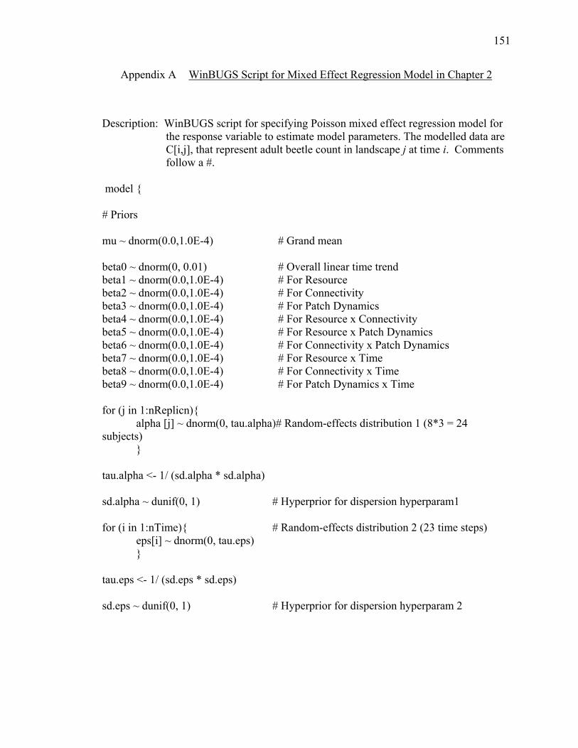
151

Appendix A WinBUGS Script for Mixed Effect Regression Model in Chapter 2

Description: WinBUGS script for specifying Poisson mixed effect regression model for the response variable to estimate model parameters. The modelled data are C[i,j], that represent adult beetle count in landscape j at time i. Comments follow a #.

model { # Priors mu ~ dnorm(0.0,1.0E-4) # Grand mean beta0 ~ dnorm(0, 0.01) # Overall linear time trend beta1 ~ dnorm(0.0,1.0E-4) # For Resource beta2 ~ dnorm(0.0,1.0E-4) # For Connectivity beta3 ~ dnorm(0.0,1.0E-4) # For Patch Dynamics beta4 ~ dnorm(0.0,1.0E-4) # For Resource x Connectivity beta5 ~ dnorm(0.0,1.0E-4) # For Resource x Patch Dynamics beta6 ~ dnorm(0.0,1.0E-4) # For Connectivity x Patch Dynamics beta7 ~ dnorm(0.0,1.0E-4) # For Resource x Time beta8 ~ dnorm(0.0,1.0E-4) # For Connectivity x Time beta9 ~ dnorm(0.0,1.0E-4) # For Patch Dynamics x Time for (j in 1:nReplicn){ alpha [j] ~ dnorm(0, tau.alpha)# Random-effects distribution 1 (8*3 = 24 subjects) } tau.alpha <- 1/ (sd.alpha * sd.alpha) sd.alpha ~ dunif(0, 1) # Hyperprior for dispersion hyperparam1 for (i in 1:nTime){ # Random-effects distribution 2 (23 time steps) eps[i] ~ dnorm(0, tau.eps) } tau.eps <- 1/ (sd.eps * sd.eps) sd.eps ~ dunif(0, 1) # Hyperprior for dispersion hyperparam 2

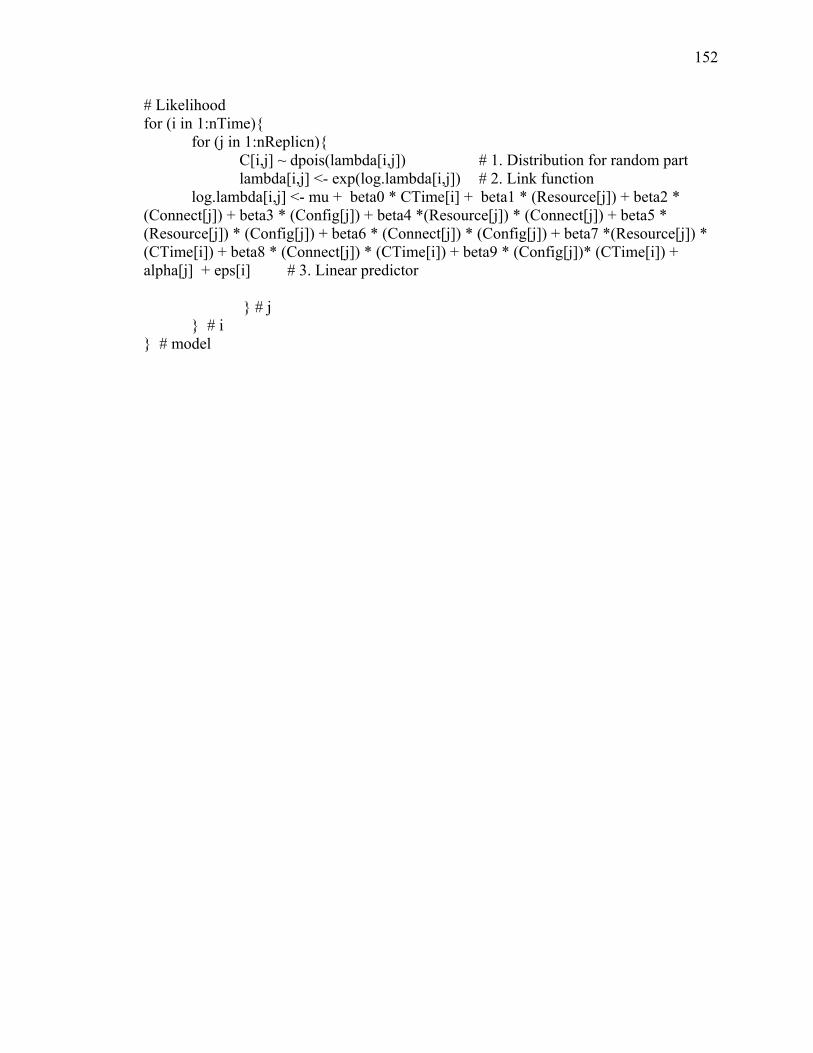
152

# Likelihood for (i in 1:nTime){ for (j in 1:nReplicn){ C[i,j] ~ dpois(lambda[i,j]) # 1. Distribution for random part lambda[i,j] <- exp(log.lambda[i,j]) # 2. Link function log.lambda[i,j] <- mu + beta0 * CTime[i] + beta1 * (Resource[j]) + beta2 * (Connect[j]) + beta3 * (Config[j]) + beta4 *(Resource[j]) * (Connect[j]) + beta5 * (Resource[j]) * (Config[j]) + beta6 * (Connect[j]) * (Config[j]) + beta7 *(Resource[j]) * (CTime[i]) + beta8 * (Connect[j]) * (CTime[i]) + beta9 * (Config[j])* (CTime[i]) + alpha[j] + eps[i] # 3. Linear predictor } # j } # i } # model

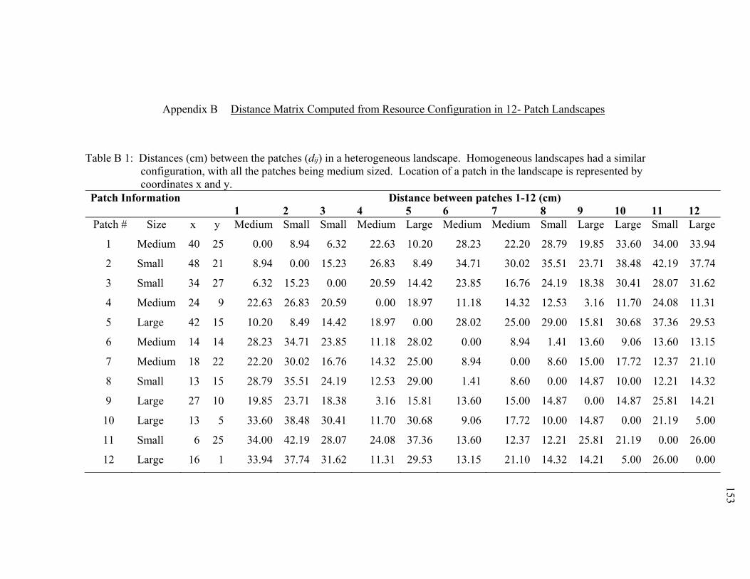
153

153

Appendix B Distance Matrix Computed from Resource Configuration in 12- Patch Landscapes

Table B 1: Distances (cm) between the patches (dij) in a heterogeneous landscape. Homogeneous landscapes had a similar configuration, with all the patches being medium sized. Location of a patch in the landscape is represented by coordinates x and y.

Patch Information Distance between patches 1-12 (cm) 1 2 3 4 5 6 7 8 9 10 11 12

Patch # Size x y Medium Small Small Medium Large Medium Medium Small Large Large Small Large

1 Medium 40 25 0.00 8.94 6.32 22.63 10.20 28.23 22.20 28.79 19.85 33.60 34.00 33.94

2 Small 48 21 8.94 0.00 15.23 26.83 8.49 34.71 30.02 35.51 23.71 38.48 42.19 37.74

3 Small 34 27 6.32 15.23 0.00 20.59 14.42 23.85 16.76 24.19 18.38 30.41 28.07 31.62

4 Medium 24 9 22.63 26.83 20.59 0.00 18.97 11.18 14.32 12.53 3.16 11.70 24.08 11.31

5 Large 42 15 10.20 8.49 14.42 18.97 0.00 28.02 25.00 29.00 15.81 30.68 37.36 29.53

6 Medium 14 14 28.23 34.71 23.85 11.18 28.02 0.00 8.94 1.41 13.60 9.06 13.60 13.15

7 Medium 18 22 22.20 30.02 16.76 14.32 25.00 8.94 0.00 8.60 15.00 17.72 12.37 21.10

8 Small 13 15 28.79 35.51 24.19 12.53 29.00 1.41 8.60 0.00 14.87 10.00 12.21 14.32

9 Large 27 10 19.85 23.71 18.38 3.16 15.81 13.60 15.00 14.87 0.00 14.87 25.81 14.21

10 Large 13 5 33.60 38.48 30.41 11.70 30.68 9.06 17.72 10.00 14.87 0.00 21.19 5.00

11 Small 6 25 34.00 42.19 28.07 24.08 37.36 13.60 12.37 12.21 25.81 21.19 0.00 26.00

12 Large 16 1 33.94 37.74 31.62 11.31 29.53 13.15 21.10 14.32 14.21 5.00 26.00 0.00

154

Appendix C Density Dependence in Emigration and Estimation of Dispersal Rate

Description: Method for estimation of density dependence of emigration rate, and for estimation of dispersal range from covariance structure in abundance, and results are presented below.

C.1 Density Dependence of Emigration Rate. I fitted a Poisson GLMM to assess the

nature of density dependence on emigration at time t in low- and high-connectivity

landscapes. Abundance of adults in the matrix at time t was regressed against the fixed

effect, the abundance of live adult beetles in patches at time t, along with random

landscape and time effects. The GLMM was implemented within a Bayesian framework.

Models were fitted in R using add-on library R2WinBUGS with 3 parallel chains.

Specification for prior and hyper prior, iterations, burn-in, thinning rate and convergence

checking were as in Govindan and Swihart (2012).

Emigration was density dependent in low connectivity landscapes (Estimate ±

SD: 0.02 ± 0.002). On the contrary, emigration was density independent in high

connectivity landscapes (0.002 ± 0.001).

C.2. Estimation of Mean Dispersal Range. Accounting for the geometry of

subpopulations, I followed the approach of Schneeberger and Jansen (2006) to estimate

the dispersal rate, the fraction of total population that disperses from one patch to another

in coupled populations experiencing equilibrium, and the per capita growth rate from the

time series data on abundance. Specifically I assumed that connectivity of patch i in a

homogenous landscape followed a negative exponential dispersal kernel such that each

off diagonal element in the connectivity matrix, exp for i j, where is

155

the dispersal range of species, a parameter that defines the distribution of dispersal

distance of focal species and are the inter-patch distances. Additionally, for each row

of the connectivity matrix, the diagonal element (i.e. i = j) was set as– ∑ ).

Accordingly, denotes the proportion of dispersers moving from patch i to patch j and

denotes the proportion reflected on the boundaries and remain in the focal patch i. For

heterogeneous landscapes, I modified exp , for all i and j, to explicitly

account for the differences in contribution of individuals from neighboring patches with

markedly different carrying capacity (area). Random values of constrained to

approximate the mean dispersal distance for beetles between 0 and 42 cm (maximum

in constructed landscape) were used in the stochastic first order auto regressive model of

the variances and covariances of the transformed abundances of time series fitted against

the eigenvalues generated from the connectivity matrix, to arrive at the best fit estimate

of dispersal range. For homogeneous landscapes, estimates of dispersal rate and related

parameters were based on time series of abundance for the first 15 time steps to better

approximate the assumption of equilibrium in metapopulations (data for t = 1 to 24 time

steps were used for heterogeneous landscapes). Confidence intervals for the dispersal

rate were estimated following the bootstrap approach (1000 runs) of Schneeberger and

Jansen (2006) . Reliable estimation of dispersal range of beetles in a landscape required

an estimate of dispersal rate to be significant (confidence interval excluded zero).

Estimated dispersal range for each replicate treatment landscape (for only those estimates

that were significant) was used in the computation of and other derived parameters for

the appropriate replicate.

156

C.3 Dispersal Range, Dispersal Rate and Per Capita Growth Rate. Estimates of per

capita growth rate (Table C.1), were influenced by the interaction effect of resource

structure and patch dynamics (Table C.2; P = 0.04). Growth rate in landscapes with fast

(vs. slow) dynamic patches was 2 times lower for homogeneous than heterogeneous

resources. Growth rate was also negatively affected by connectivity (Table C.2; P =

0.04); it was 30% higher in low (0.52 ± 0.04) versus high (0.40 ± 0. 03) connectivity

landscapes (Table C.1). For a given resource structure, landscapes with low connectivity

and slow dynamics had the highest growth rates, with beetle populations in

heterogeneous landscapes growing slightly faster (P < 0.10). The low connectivity and

slow dynamic landscapes exhibited greater growth rates (P < 0.05) than any other

treatment containing homogeneous resources (Table C.1).

The estimate of species’ dispersal rate was significant (95% confidence interval

excluded zero) for all replicate homogeneous landscapes. In contrast, except for the high

connectivity slow dynamic counterpart, only two of three replicates for each of the

heterogeneous landscape treatments were different from zero. For the corresponding

heterogeneous treatments, nonsignificant replicates were ignored while computing

metapopulation capacity and derived parameters. Resource structure had a negative

effect (P << 0.001) and connectivity a positive effect (P = 0.04) on patch-specific

dispersal rate (Table C.2). Dispersal rate of beetles was significantly lower in

heterogeneous (0.04 ± 0.01) than homogeneous (0.11 ± 0.01) landscapes and in low (0.05

± 0.01) than high connectivity (0.09 ± 0.01) landscapes (Table C.1). Consistent with

these results and differences in growth rates evinced in these landscapes, connectivity had

a significant effect on adult beetle mortality in the matrix (P << 0.001) as well as inside

157

the patches (P << 0.001; Table C.1). While mortality in the matrix was 46% higher in

high (vs. low) connectivity landscapes, mortality inside the patches was only 20% higher

in landscapes with low (vs. high) connectivity.

Dispersal range of beetles in the landscape tended to be affected by an interaction

of resource structure and patch connectivity (P = 0.05) and also by resource structure and

patch dynamics (P = 0.09) (Table C.2). Lower connectivity as well as slower dynamics

dampened the dispersal range in heterogeneous resource landscapes as opposed to their

homogeneous counterparts. in heterogeneous versus homogeneous resource

landscapes was 2.2 times less with low than high patch connectivity. Similarly, in

landscape with heterogeneous versus homogeneous resource was 2.4 times less with low

than high connectivity.

Landscapes with heterogeneous resources, low connectivity and slow patch

dynamics exhibited the highest per patch growth rate, an intermediate and less variable

and lowest dispersal rate (Table C.1). in this landscape was distinctly lower than that

in other heterogeneous landscapes (P < 0.01) except for the analogous fast dynamic

landscape (P = 0.43; Table C.1). In contrast, it was not different from homogeneous

landscapes except for the low connectivity slow dynamic counterpart, that exhibited the

highest dispersal range, highest growth rate and lowest dispersal rate (P = 0.01; Table C.1)

among homogeneous ones.

158

Table C 1: Estimate (mean) of species specific attributes for the eight treatment landscapes. Standard deviation of estimate is presented in parenthesis. For each parameter, treatment means with same superscript are not different from each other (Tukey sandwich HSD, P < 0.05). Abundance data from time steps t = 0 to 15 and t = 0 to 23 were used in the estimation of species specific attributes for homogeneous and heterogeneous landscapes, respectively.

Treat- ment #

Resource Structure

Patch Connectivity

Patch Dynamics

Growth Rate

Dispersal Range

Dispersal Rate

1 Homogeneous High Fast 0.30cd (0.07)

0.04ab (0.02)

0.14c (0.04)

2 Homogeneous High Slow 0.37cb (0.03)

0.05ab (0.02)

0.10c (0.02)

3 * Homogeneous Low Fast 0.26d (0.06)

0.03a (0.00)

0.13c (0.04)

4 Homogeneous Low Slow 0.50ab (0.08)

0.06b (0.01)

0.09bc (0.04)

5 ** Heterogeneous High Fast 0.46b (0.08)

0.17c (0.02)

0.04ab (0.03)

6 Heterogeneous High Slow 0.49ab (0.08)

0.19c (0.07)

0.06abc (0.04)

7 ** Heterogeneous Low Fast 0.62a (0.04)

0.17abc (0.13)

0.02ab (0.04)

8 ** Heterogeneous Low Slow 0.63a (0.01)

0.04a (0.01)

0.01a (0.02)

* or ** Mean ± SD is based on two replicates [* One replicate for this treatment (#3) suffered fungal infestation, and ** 95% credible interval for the dispersal rate estimated for one replicate each for these treatments (#5, #7 and #8) contained zero; data from corresponding replicates were not included in analysis].

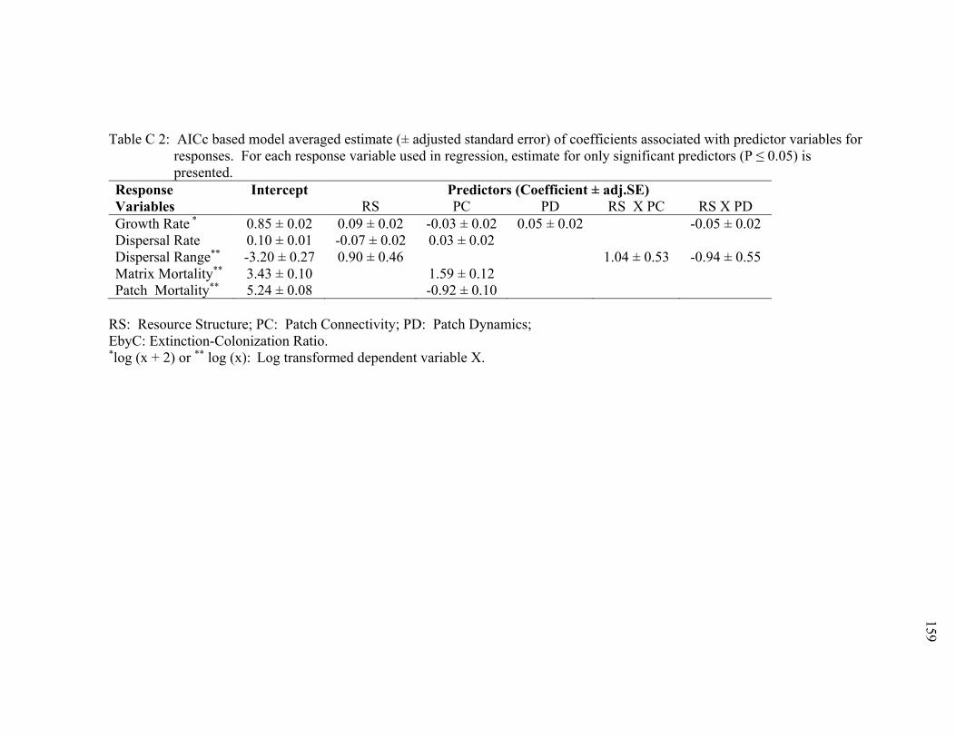
159

159

Table C 2: AICc based model averaged estimate (± adjusted standard error) of coefficients associated with predictor variables for responses. For each response variable used in regression, estimate for only significant predictors (P ≤ 0.05) is presented.

Response Variables

Intercept Predictors (Coefficient ± adj.SE) RS PC PD RS X PC RS X PD

Growth Rate * 0.85 ± 0.02 0.09 ± 0.02 -0.03 ± 0.02 0.05 ± 0.02 -0.05 ± 0.02 Dispersal Rate 0.10 ± 0.01 -0.07 ± 0.02 0.03 ± 0.02 Dispersal Range** -3.20 ± 0.27 0.90 ± 0.46 1.04 ± 0.53 -0.94 ± 0.55 Matrix Mortality** 3.43 ± 0.10 1.59 ± 0.12 Patch Mortality** 5.24 ± 0.08 -0.92 ± 0.10

RS: Resource Structure; PC: Patch Connectivity; PD: Patch Dynamics; EbyC: Extinction-Colonization Ratio. *log (x + 2) or ** log (x): Log transformed dependent variable X.

160

160

Appendix D Distribution of Circle Traps and Curculio Species Abundance on Host Trees in 2005-2008

Table D 1: Circle traps partitioned by host tree species, location in forest stands (core/edge class) and year. Grand total column denotes total number of hosts per tree species for which detection data (along with missing data) on weevils from 2005-08 was used in this study.

Host Tree Species

2005 2006 2007 2008 Grand Total Core Edge Total Core Edge Total Core Edge Total Core Edge Total

Red Oak 15 13 28 33 28 61 42 32 74 42 32 74 74 White Oak 22 18 40 45 44 89 52 48 100 52 47 99 100

SubTotal 37 31 68 78 72 150 94 80 174 94 79 173 174

Table D 2: Captures of different Curculio weevil species partitioned by year, host tree species and location (core/edge class) in

forest stands.

Weevil Species

Host Tree Species

2005 2006 2007 2008 Grand Total Core Edge Total Core Edge Total Core Edge Total Core Edge Total

C.pardalis Red oak 19 7 26 6 3 9 122 43 165 3 7 10 210 White oak 76 53 129 7 6 13 262 364 626 36 41 77 845

SubTotal 95 60 155 13 9 22 384 407 791 39 48 87 1055

C.sulcatulus Red oak 7 1 8 76 41 117 110 34 144 52 33 85 354 White oak 20 11 31 37 40 77 38 19 57 44 32 76 241 SubTotal 27 12 39 113 81 194 148 53 201 96 65 161 595

161

161

Table D.2, Continued

C.proboscideus Redoak 23 3 26 137 45 182 86 39 125 147 60 207 540 White oak 19 17 36 38 23 61 61 20 81 54 45 99 277 SubTotal 42 20 62 175 68 243 147 59 206 201 105 306 817

Total 164 92 256 301 158 459 679 519 1198 336 218 554 2467

162

Appendix E WinBUGS Script for Single-Species Multi-Season Occupancy Model

Description: WinBUGS script for specifying occupancy dynamics model incorporating season and survey specific covariates for detection probability and season and site specific covariates for occupancy and local vital rates to estimate model and derived parameters. The modelled data are x[j,i,k], which contain the detection/non-detection (1/0) observations of a species in year j, site i and replicate survey k. The first 100 sites denote white oaks followed by 74 red oaks. Comments follow a #.

model { # Specify prior distributions for model parameters beta0~dunif(-8,8) # Intercept of covariate effect on 1st-year occupancy beta2~dunif(-10,10) # Slope of covariate (mast)effect on 1st-year occupancy beta5~dunif(-8,8) # Slope of covariate (FD100)effect on 1st-year occupancy beta6~dunif(-8,8) # Slope of covariate (WO)effect on 1st-year occupancy beta9~dunif(-12,12) # Slope of covariate (WO*mast)effect on 1st-year

occupancy lphi0~dunif(-12,12) # Intercept of covariate effect on survival lgamma0~dunif(-12,12) # Intercept of covariate effect on colonization lphi2~dunif(-12,12) # Slope of covariate (mast) effect on survival lgamma2~dunif(-12,12) # Slope of covariate (mast)effect on colonization lphi5~dunif(-13,13) # Slope of covariate (FD100) effect on survival lgamma5~dunif(-13,13) # Slope of covariate (FD100)effect on colonization lphi6~dunif(-12,12) # Slope of covariate (WO)effect on survival lgamma6~dunif(-12,12) # Slope of covariate(WO)effect on colonization lphi9~dunif(-12,12) # Slope of covariate (WO*mast)effect on survival lgamma9~dunif(-12,12) # Slope of covariate(WO*mast)effect on colonization for(i in 1:nyear){ alpha0[i]~ dunif(-12,12) # Intercept of date effect on p alpha1[i]~ dunif(-12,12) # Linear effect of date on p alpha2[i]~ dunif(-12,12) # Quadratic effect of date on p } # (Part of) Observation submodel: Define structure for p for(i in 1:nsite){ for(j in 1:nyear){ for(k in 1:REPS[i,j]){ logit(pmat[j,i,k])<- alpha0[j] + alpha1[j] * date[j,i,k] + alpha2[j] * pow(date[j,i,k], 2) } } }

163

# State submodel # initial state and likelihood for year = 1 for(i in 1:nsite){ z[i,1]~dbern(psi[i,1]) # Logit-linear covariate effect on first-year occupancy logit(psi[i,1]) <- beta0 + beta6 * whiteoak[i] + beta2 * mast[i,1] + beta5 * FD100[i] + beta9 * whiteoak[i]* mast[i,1] for(k in 1:REPS[i,1]){ mu2[1,i,k]<-z[i,1]*pmat[1,i,k] x[1,i,k] ~ dbern(mu2[1,i,k]) } } # for years 2 through nyear for(i in 1:nsite){ for(j in 2:nyear){ # Logit-linear covariate effects on occupancy dynamics logit(phi[i,j-1]) <- lphi0 + lphi6 * whiteoak[i] + lphi2 * mast[i,j] + lphi5 * FD100[i] + lphi9 * whiteoak[i]* mast[i,j] # Survival logit(gamma[i,j-1]) <- lgamma0 + lgamma6 * whiteoak[i] + lgamma2 * mast[i,j] + lgamma5 * FD100[i] + lgamma9 * whiteoak[i]* mast[i,j] # Colonization mu[i,j]<-z[i,j-1]*phi[i,j-1]+ (1-z[i,j-1])*gamma[i,j-1] z[i,j]~dbern(mu[i,j]) # Observation model: likelihood for the observed data for(k in 1:REPS[i,j]){ mu2[j,i,k]<-z[i,j]*pmat[j,i,k] x[j,i,k]~dbern(mu2[j,i,k]) } } } #Psi at host tree level to derive white oak and red oak specific parameters for(i in 1:nsite){ for(j in 2:nyear){ psi[i,j] <- psi[i,j-1]*phi[i,j-1]+ (1-psi[i,j-1])*gamma[i,j-1] } } # Derived parameters: Compute annual occupancy and growthrates psivec[1]<- mean(psi[1:174,1])

164

psi.fs[1]<-sum(z[1:nsite,1])/nsite for(q in 1:nyear){ psiWR[q]<- mean(psi[1:174,q]) psiwhite[q]<- mean(psi[1:100,q]) psired[q]<- mean(psi[101:174,q]) } for(q in 1:(nyear-1)){ phiyr[q]<-mean(phi[1:174,q]) gammayr[q]<-mean(gamma[1:174,q]) phiWR[q]<- mean(phi[1:174,q]) phiwhite[q]<- mean(phi[1:100,q]) phired[q]<- mean(phi[101:174,q]) gammaWR[q]<- mean(gamma[1:174,q]) gammawhite[q]<- mean(gamma[1:100,q]) gammared[q]<- mean(gamma[101:174,q]) } for(j in 2:nyear){ psivec[j] <- psivec[j-1]*phiyr[j-1]+ (1-psivec[j-1])*gammayr[j-1] growthr[j]<- psivec[j]/psivec[j-1] psi.fs[j]<-sum(z[1:nsite,j])/nsite turnover[j-1]<- ((1 - psivec[j-1]) * gammayr[j-1])/( (1 - psivec[j-1]) * gammayr[j-1] + phiyr[j-1]*psivec[j-1]) eop[j-1]<- (gammayr[j-1])/( (gammayr[j-1])+ (1-phiyr[j-1])) } } # end of model.

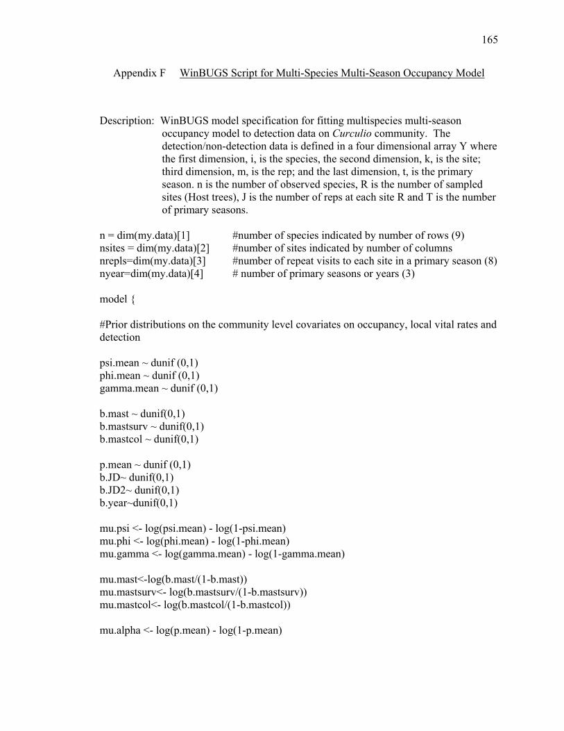
165

Appendix F WinBUGS Script for Multi-Species Multi-Season Occupancy Model

Description: WinBUGS model specification for fitting multispecies multi-season occupancy model to detection data on Curculio community. The detection/non-detection data is defined in a four dimensional array Y where the first dimension, i, is the species, the second dimension, k, is the site; third dimension, m, is the rep; and the last dimension, t, is the primary season. n is the number of observed species, R is the number of sampled sites (Host trees), J is the number of reps at each site R and T is the number of primary seasons.

n = dim(my.data)[1] #number of species indicated by number of rows (9) nsites = dim(my.data)[2] #number of sites indicated by number of columns nrepls=dim(my.data)[3] #number of repeat visits to each site in a primary season (8) nyear=dim(my.data)[4] # number of primary seasons or years (3) model { #Prior distributions on the community level covariates on occupancy, local vital rates and detection psi.mean ~ dunif (0,1) phi.mean ~ dunif (0,1) gamma.mean ~ dunif (0,1) b.mast ~ dunif(0,1) b.mastsurv ~ dunif(0,1) b.mastcol ~ dunif(0,1) p.mean ~ dunif (0,1) b.JD~ dunif(0,1) b.JD2~ dunif(0,1) b.year~dunif(0,1) mu.psi <- log(psi.mean) - log(1-psi.mean) mu.phi <- log(phi.mean) - log(1-phi.mean) mu.gamma <- log(gamma.mean) - log(1-gamma.mean) mu.mast<-log(b.mast/(1-b.mast)) mu.mastsurv<- log(b.mastsurv/(1-b.mastsurv)) mu.mastcol<- log(b.mastcol/(1-b.mastcol)) mu.alpha <- log(p.mean) - log(1-p.mean)

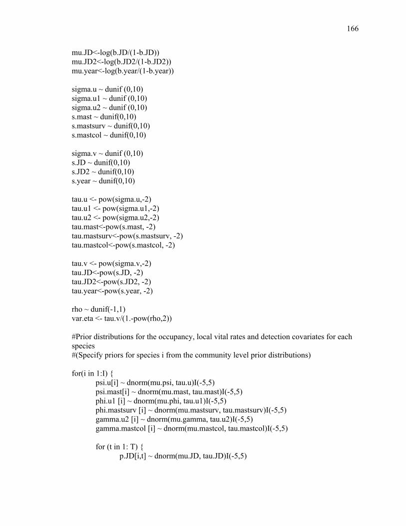
166

mu.JD<-log(b.JD/(1-b.JD)) mu.JD2<-log(b.JD2/(1-b.JD2)) mu.year<-log(b.year/(1-b.year)) sigma.u ~ dunif (0,10) sigma.u1 ~ dunif (0,10) sigma.u2 ~ dunif (0,10) s.mast ~ dunif(0,10) s.mastsurv ~ dunif(0,10) s.mastcol ~ dunif(0,10) sigma.v ~ dunif (0,10) s.JD ~ dunif(0,10) s.JD2 ~ dunif(0,10) s.year ~ dunif(0,10) tau.u <- pow(sigma.u,-2) tau.u1 <- pow(sigma.u1,-2) tau.u2 <- pow(sigma.u2,-2) tau.mast<-pow(s.mast, -2) tau.mastsurv<-pow(s.mastsurv, -2) tau.mastcol<-pow(s.mastcol, -2) tau.v <- pow(sigma.v,-2) tau.JD<-pow(s.JD, -2) tau.JD2<-pow(s.JD2, -2) tau.year<-pow(s.year, -2) rho ~ dunif(-1,1) var.eta <- tau.v/(1.-pow(rho,2)) #Prior distributions for the occupancy, local vital rates and detection covariates for each species #(Specify priors for species i from the community level prior distributions) for(i in 1:I) { psi.u[i] ~ dnorm(mu.psi, tau.u)I(-5,5) psi.mast[i] ~ dnorm(mu.mast, tau.mast)I(-5,5) phi.u1 [i] ~ dnorm(mu.phi, tau.u1)I(-5,5) phi.mastsurv [i] ~ dnorm(mu.mastsurv, tau.mastsurv)I(-5,5) gamma.u2 [i] ~ dnorm(mu.gamma, tau.u2)I(-5,5) gamma.mastcol [i] ~ dnorm(mu.mastcol, tau.mastcol)I(-5,5) for (t in 1: T) { p.JD[i,t] ~ dnorm(mu.JD, tau.JD)I(-5,5)

167

p.JD2[i,t] ~ dnorm(mu.JD2, tau.JD2)I(-5,5) } } for (t in 1:T){ p.year[t]~dnorm(mu.year, tau.year)I(-5,5) } for(i in 1:I){ mu.eta[i] <- mu.alpha + (rho*sigma.v/sigma.u)*(psi.u[i] - mu.psi) eta[i] ~ dnorm(mu.eta[i], var.eta)I(-5,5) } # at logit(psi),add occupancy covariates and for logit(p),add detection covariates for (i in 1:I){ #for I species for (k in 1:K) { # for K sites for (t in 1:T){ # for T primary seasons for (m in 1:M){ # for M replicate visits #Part of observation submodel : Define structure for p #(Estimate the species specific detection probability 'p' for every replicate visit at each site, where the species occurs (Z=1)) logit(p[i,k,m,t]) <- eta[i] + p.JD[i,t]*c.JD[k,m,t]+ p.JD2[i,t]*c.JD2[k,m,t]+ p.year[t] } } } } #State Submodel (#Estimate of the first year occupancy probability (latent Z matrix) for each species at each site) # initial state and likelihood for year = 1 for (i in 1:I){ #for I species for (k in 1:K) { # for K sites # for (t in 1:1){ # for first primary season logit(psi[i,k]) <- psi.u[i]+ psi.mast[i]* c.mast[k,1] Z[i,k,1] ~ dbern(psi[i,k]) for (m in 1:M){# for M replicate visits mu.p[i,k,m,1] <- p[i,k,m,1]*Z[i,k,1] Y[i,k,m,1] ~ dbern(mu.p[i,k,m,1]) Ynew[i,k,m,1] ~ dbern(mu.p[i,k,m,1]) } #} } } # for year 2 to 3 for (i in 1:I){ #for I species

168

for (k in 1:K) { # for K sites for (t in 2:T){ # for 2nd to 3rd primary season # Logit-linear covariate effects on occupancy dynamics logit(phisurv[i,k,t-1]) <- phi.u1[i] + phi.mastsurv [i] * c.mast[k,t] logit(gamma[i,k,t-1]) <- gamma.u2[i] + gamma.mastcol[i] * c.mast[k,t] mu[i,k,t]<-Z[i,k,t-1]*phisurv[i,k,t-1]+ (1-Z[i,k,t-1])*gamma[i,k,t-1] Z[i,k,t]~dbern(mu[i,k,t]) # Observation model: likelihood for the observed data for(m in 1: M){ # for M replicate visits mu.p[i,k,m,t]<-p[i,k,m,t]*Z[i,k,t] Y[i,k,m,t]~dbern(mu.p[i,k,m,t]) Ynew[i,k,m,t]~dbern(mu.p[i,k,m,t]) } } } } for (i in 1:I){ #for I species for (k in 1:K) { # for K sites for (t in 1:T){ # for T primary seasons for(m in 1: M) { # for M replicate visits #Create simulated dataset to calculate the Bayesian p-value d[i,k,m,t]<- abs(Y[i,k,m,t] - mu.p[i,k,m,t]) dnew[i,k,m,t]<- abs(Ynew[i,k,m,t] - mu.p[i,k,m,t]) d2[i,k,m,t]<- pow(d[i,k,m,t],2) dnew2[i,k,m,t]<- pow(dnew[i,k,m,t],2) } dsum[i,k,t]<- sum(d2[i,k,1:M,t]) dnewsum[i,k,t]<- sum(dnew2[i,k,1:M,t]) } } } #Calculate the discrepancy measure, which is then defined as the mean(p.fit > p.fitnew) p.fit<-sum(dsum[1:I,1:K,1:T]) p.fitnew<-sum(dnewsum[1:I,1:K,1:T]) # Derived parameters: Compute annual occupancy, growthrates, turnover and eop for(i in 1:I){ psivec[i,1]<- mean(psi[i,1:K]) for(t in 1:2) { phiyr[i,t]<-mean(phisurv[i,1:K,t]) gammayr[i,t]<-mean(gamma[i,1:K,t])

169

} } for(i in 1:I){ for(t in 2:T){ psivec[i,t] <- psivec[i,t-1]*phiyr[i,t-1]+ (1-psivec[i,t-1])*gammayr[i,t-1] growthr[i,t]<- psivec[i,t]/psivec[i,t-1] turnover[i,t-1]<- ((1 - psivec[i,t-1]) * gammayr[i,t-1])/( (1 - psivec[i,t-1]) * gammayr[i,t-1] + phiyr[i,t-1]*psivec[i,t-1]) eop[i,t-1]<- (gammayr[i,t-1])/( (gammayr[i,t-1])+ (1-phiyr[i,t-1])) } } #Species-richness N as a derived parameter for (t in 1:T){ YearSR[t] <-sum(Z[,,t])/K for (k in 1:K){ SiteSR[k,t] <-sum(Z[,k,t]) } } }

170

170

Appendix G Patch Occupancy and Vital Rates for Nine Curculio spp. from Single-Species Multi-Season Occupancy Models

Table G 1: Annual site occupancy for the nine species of Curculio weevils with all host tree species considered (red oak, white oak and shagbark hickory) and corresponding 95% credible intervals, estimated from single-species occupancy models. Year is indexed in brackets as1-3 and corresponds to 2006-2008, respectively. Survival and colonization rates for each Curculio species correspond to 2006-07 and 2007-08.

Species All Hosts (Single-Species Multi-Season Model)

Year Apparent Occupancy

Estimated Occupancy

Survival Probability

Colonization Probability

C. caryae 1 0.00 0.63 (0.10 – 0.91) 0.81 (0.48 – 0.92) 0.40 (0.05 – 0.92) C. caryae 2 0.07 0.70 (0.52 – 0.86) 0.61 (0.34 – 0.78) 0.32 (0.04 – 0.88) C. caryae 3 0.40 0.51 (0.43 – 0.60) C. confusor 1 0.02 0.61 (0.13 – 0.92) 0.39 (0.15 – 0.84) 0.46 (0.19 – 0.71) C. confusor 2 0.25 0.38 (0.28 – 0.49) 0.44 (0.28 – 0.67) 0.30 (0.17 – 0.43) C. confusor 3 0.25 0.35 (0.28 – 0.44) C. iowensis 1 0.004 0.48 (0.15 – 0.84) 0.46 (0.13 – 0.85) 0.45 (0.13 – 0.86) C. iowensis 2 0.003 0.45 (0.16 – 0.79) 0.50 (0.10 – 0.90) 0.47 (0.09 – 0.90) C. iowensis 3 0.00 0.48 (0.15 – 0.81) C. nasicus 1 0.16 0.40 (0.21 – 0.71) 0.63 (0.26 – 0.99) 0.11 (0.01 – 0.42) C. nasicus 2 0.09 0.31 (0.14 – 0.60) 0.47 (0.11 – 0.98) 0.12 (0.01 – 0.34) C. nasicus 3 0.04 0.25 (0.07 – 0.61) C. orthorhynchus 1 0.08 0.31 (0.20 – 0.48) 0.65 (0.37 – 0.92) 0.08 (0.05 – 0.15) C. orthorhynchus 2 0.12 0.26 (0.16 – 0.39) 0.49 (0.23 – 0.87) 0.15 (0.07 – 0.28) C. orthorhynchus 3 0.08 0.24 (0.13 – 0.42)

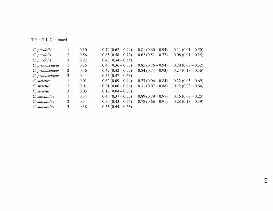
171

171

Table G.1, Continued

C. pardalis 1 0.10 0.79 (0.62 – 0.99) 0.81 (0.60 – 0.94) 0.11 (0.01 – 0.50) C. pardalis 2 0.56 0.65 (0.58 – 0.72) 0.62 (0.51 – 0.77) 0.08 (0.01 – 0.25) C. pardalis 3 0.22 0.43 (0.34 – 0.55) C. proboscideus 1 0.35 0.45 (0.36 – 0.55) 0.85 (0.76 – 0.94) 0.20 (0.08 – 0.32) C. proboscideus 2 0.36 0.49 (0.42 – 0.57) 0.84 (0.74 – 0.93) 0.27 (0.18 – 0.36) C. proboscideus 3 0.44 0.55 (0.47 – 0.63) C. strictus 1 0.01 0.62 (0.09 – 0.94) 0.23 (0.06 – 0.84) 0.22 (0.05 – 0.69) C. strictus 2 0.01 0.21 (0.06 – 0.66) 0.31 (0.07 – 0.88) 0.12 (0.03 – 0.64) C. strictus 3 0.03 0.16 (0.04 – 0.60) C. sulcatulus 1 0.34 0.46 (0.37 – 0.55) 0.89 (0.79 – 0.97) 0.16 (0.08 – 0.25) C. sulcatulus 2 0.34 0.50 (0.43 – 0.56) 0.78 (0.66 – 0.91) 0.28 (0.18 – 0.39) C. sulcatulus 3 0.38 0.53 (0.44 – 0.63)

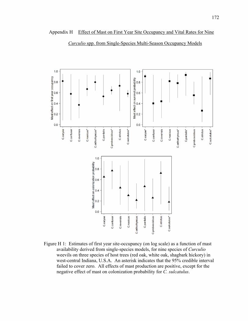
172

Appendix H Effect of Mast on First Year Site Occupancy and Vital Rates for Nine

Curculio spp. from Single-Species Multi-Season Occupancy Models

Figure H 1: Estimates of first year site-occupancy (on log scale) as a function of mast availability derived from single-species models, for nine species of Curculio weevils on three species of host trees (red oak, white oak, shagbark hickory) in west-central Indiana, U.S.A. An asterisk indicates that the 95% credible interval failed to cover zero. All effects of mast production are positive, except for the negative effect of mast on colonization probability for C. sulcatulus.

173

Appendix I Effect of Mast on Vital Rates for Nine Curculio spp. from Multi-Species

Multi-Season Occupancy Models

Figure I 1: Estimates of survival (filled square) and colonization (filled triangle) probability (on log scale) as a function of mast availability derived from multi-species occupancy model for 9 species of Curculio weevils on white and red oak species of host trees in west-central Indiana, U.S.A. Curculio species index on abscissa followed by ‘*’ means 95% credible interval did not contain zero, whereas a † signifies that a fraction, f, of the posterior distribution was more extreme than zero (see text).

174

Appendix J Annual Site Occupancy for the Nine Species of Curculio spp. Multi-

Species Multi-Season Occupancy Models

Table J 1: Annual site occupancy for the nine species of Curculio weevils on host tree species and corresponding 95% posterior credible intervals from multi-species occupancy models. Year index 1-3 corresponds to 2006-2008 respectively. ‘All hosts’ model is based on detection data for weevils on 3 host tree species: red oak, white oak and shagbark hickory.

Curculio Occupancy (Multi-Species Multi-Season Model)

Year All Hosts White Oak Red Oak C. caryae 1 0.04 (0.01 – 0.13) 0.10 (0.01 – 0.35) 0.14 (0.01 – 0.54)C. caryae 2 0.48 (0.35 – 0.69) 0.40 (0.22 – 0.74) 0.45 (0.19 – 0.85)C. caryae 3 0.50 (0.42 – 0.60) 0.48 (0.32 – 0.70) 0.45 (0.23 – 0.79)C. confusor 1 0.05 (0.02 – 0.10) 0.09 (0.02 – 0.22) 0.10 (0.01 – 0.31)C. confusor 2 0.37 (0.30 – 0.46) 0.57 (0.42 – 0.83) 0.47 (0.24 – 0.89)C. confusor 3 0.42 (0.33 – 0.53) 0.49 (0.37 – 0.64) 0.46 (0.21 – 0.83)C. iowensis 1 0.17 (0.01 – 0.86) 0.43 (0.03 – 0.97) 0.22 (0.01 – 0.92)C. iowensis 2 0.20 (0.02 – 0.70) 0.52 (0.07 – 0.89) 0.33 (0.03 – 0.88)C. iowensis 3 0.19 (0.02 – 0.64) 0.44 (0.06 – 0.81) 0.26 (0.02 – 0.82)C. nasicus 1 0.39 (0.25 – 0.60) 0.55 (0.22 – 0.97) 0.66 (0.40 – 0.96)C. nasicus 2 0.24 (0.14 – 0.39) 0.50 (0.16 – 0.87) 0.43 (0.23 – 0.71)C. nasicus 3 0.13 (0.07 – 0.25) 0.37 (0.09 – 0.74) 0.20 (0.07 – 0.45)C. orthorhynchus 1 0.21 (0.10 – 0.38) 0.45 (0.14 – 0.94) 0.34 (0.14 – 0.55)C. orthorhynchus 2 0.26 (0.17 – 0.38) 0.62 (0.32 – 0.92) 0.42 (0.27 – 0.58)C. orthorhynchus 3 0.26 (0.15 – 0.41) 0.55 (0.28 – 0.86) 0.35 (0.18 – 0.54)C. pardalis 1 0.13 (0.09 – 0.19) 0.17 (0.09 – 0.28) 0.25 (0.11 – 0.45)C. pardalis 2 0.59 (0.51 – 0.68) 0.75 (0.64 – 0.88) 0.79 (0.58 – 0.94)C. pardalis 3 0.48 (0.41 – 0.55) 0.51 (0.41 – 0.61) 0.49 (0.27 – 0.83)C. proboscideus 1 0.43 (0.36 – 0.51) 0.36 (0.24 – 0.51) 0.72 (0.60 – 0.83)C. proboscideus 2 0.49 (0.43 – 0.56) 0.54 (0.42 – 0.66) 0.78 (0.68 – 0.87)C. proboscideus 3 0.53 (0.46 – 0.62) 0.57 (0.44 – 0.71) 0.75 (0.63 – 0.86)C. strictus 1 0.15 (0.02 – 0.65) 0.22 (0.01 – 0.89) 0.50 (0.10 – 0.97)C. strictus 2 0.17 (0.04 – 0.63) 0.42 (0.07 – 0.89) 0.42 (0.06 – 0.90)C. strictus 3 0.17 (0.04 – 0.60) 0.41 (0.09 – 0.81) 0.31 (0.02 – 0.86)C. sulcatulus 1 0.45 (0.38 – 0.54) 0.42 (0.30 – 0.56) 0.76 (0.64 – 0.87)C. sulcatulus 2 0.50 (0.43 – 0.56) 0.57 (0.45 – 0.69) 0.74 (0.64 – 0.84)C. sulcatulus 3 0.49 (0.41 – 0.57) 0.59 (0.45 – 0.74) 0.61 (0.46 – 0.75)

175

Table J 2: Site-specific vital rates for the nine Curculio species and the 95% credible intervals from multi-species models.

Curculio Sps. Survival (Multi-Species Multi-Season Model) Year All Hosts White Oak Red Oak

C. caryae 2006-07 0.80 (0.65 – 0.92) 0.84 (0.53 – 0.97) 0.82 (0.38 – 0.99)C. caryae 2007-08 0.58 (0.40 – 0.81) 0.68 (0.37 – 0.96) 0.69 (0.21 – 0.98)C. confusor 2006-07 0.72 (0.36 – 0.90) 0.82 (0.61 – 0.91) 0.79 (0.36 – 0.98)C. confusor 2007-08 0.56 (0.38 – 0.77) 0.52 (0.34 – 0.71) 0.65 (0.21 – 0.98)C. iowensis 2006-07 0.64 (0.12 – 0.96) 0.78 (0.34 – 0.96) 0.65 (0.08 – 0.98)C. iowensis 2007-08 0.51 (0.05 – 0.95) 0.60 (0.13 – 0.95) 0.50 (0.01 – 0.98)C. nasicus 2006-07 0.49 (0.26 – 0.78) 0.76 (0.23 – 0.94) 0.50 (0.24 – 0.81)C. nasicus 2007-08 0.30 (0.11 – 0.59) 0.58 (0.22 – 0.89) 0.20 (0.03 – 0.58)C. orthorhynchus 2006-07 0.78 (0.56 – 0.96) 0.83 (0.52 – 0.97) 0.88 (0.68 – 0.99)C. orthorhynchus 2007-08 0.63 (0.33 – 0.93) 0.62 (0.18 – 0.94) 0.75 (0.39 – 0.98)C. pardalis 2006-07 0.74 (0.60 – 0.84) 0.84 (0.75 – 0.90) 0.74 (0.48 – 0.95)C. pardalis 2007-08 0.46 (0.37 – 0.57) 0.49 (0.38 – 0.62) 0.46 (0.18 – 0.90)C. proboscideus 2006-07 0.84 (0.75 – 0.92) 0.85 (0.66 – 0.96) 0.96 (0.90 – 0.99)C. proboscideus 2007-08 0.82 (0.73 – 0.91) 0.74 (0.54 – 0.92) 0.92 (0.82 – 0.98)C. strictus 2006-07 0.64 (0.16 – 0.95) 0.82 (0.49 – 0.97) 0.58 (0.06 – 0.98)C. strictus 2007-08 0.56 (0.12 – 0.94) 0.63 (0.25 – 0.96) 0.44 (0.01 – 0.97)C. sulcatulus 2006-07 0.85 (0.76 – 0.93) 0.87 (0.74 – 0.95) 0.90 (0.81 – 0.96)C. sulcatulus 2007-08 0.75 (0.64 – 0.86) 0.68 (0.50 – 0.89) 0.79 (0.64 – 0.92)

Colonization (Multi-Species Multi-Season Model) C. caryae 2006-07 0.47 (0.32 – 0.69) 0.35 (0.15 – 0.73) 0.39 (0.10 – 0.87)C. caryae 2007-08 0.45 (0.31 – 0.67) 0.37 (0.18 – 0.69) 0.29 (0.05 – 0.83)C. confusor 2006-07 0.35 (0.28 – 0.44) 0.55 (0.39 – 0.84) 0.44 (0.19 – 0.92)C. confusor 2007-08 0.33 (0.26 – 0.43) 0.48 (0.31 – 0.78) 0.32 (0.11 – 0.87)C. iowensis 2006-07 0.12 (0.01 – 0.55) 0.35 (0.01 – 0.87) 0.27 (0.01 – 0.89)C. iowensis 2007-08 0.13 (0.01 – 0.55) 0.35 (0.01 – 0.89) 0.18 (0.00 – 0.86)C. nasicus 2006-07 0.07 (0.02 – 0.17) 0.22 (0.01 – 0.68) 0.29 (0.04 – 0.70)C. nasicus 2007-08 0.07 (0.02 – 0.16) 0.20 (0.01 – 0.68) 0.18 (0.02 – 0.51)C. orthorhynchus 2006-07 0.11 (0.03 – 0.23) 0.45 (0.08 – 0.94) 0.17 (0.01 – 0.44)C. orthorhynchus 2007-08 0.12 (0.03 – 0.24) 0.49 (0.08 – 0.95) 0.06 (0.00 – 0.19)C. pardalis 2006-07 0.57 (0.48 – 0.67) 0.73 (0.60 – 0.90) 0.81 (0.52 – 0.99)C. pardalis 2007-08 0.50 (0.40 – 0.63) 0.57 (0.36 – 0.86) 0.70 (0.29 – 0.98)C. proboscideus 2006-07 0.24 (0.14 – 0.32) 0.36 (0.19 – 0.52) 0.32 (0.09 – 0.57)C. proboscideus 2007-08 0.25 (0.18 – 0.33) 0.38 (0.24 – 0.55) 0.14 (0.02 – 0.31)C. strictus 2006-07 0.10 (0.01 – 0.41) 0.33 (0.03 – 0.88) 0.28 (0.01 – 0.90)C. strictus 2007-08 0.10 (0.01 – 0.43) 0.32 (0.03 – 0.89) 0.20 (0.01 – 0.89)C. sulcatulus 2006-07 0.20 (0.12 – 0.28) 0.35 (0.21 – 0.52) 0.21 (0.02 – 0.49)C. sulcatulus 2007-08 0.23 (0.15 – 0.32) 0.46 (0.29 – 0.68) 0.09 (0.01 – 0.25)

176

VITA

176

VITA

Byju Nambidiyattil Govindan Department of Forestry and Natural Resources, Purdue University

715 W. State Street, West Lafayette, Indiana, 47907 Education Ph.D, Ecology, 2013, Forestry & Natural Resources (FNR), Purdue University, IN MS, Technology, 2013, Computer & Information Technology, Purdue University, IN M. Sc., Agricultural Entomology, 2003, University of Agricultural Sciences(B), India B.Sc., Agriculture, 2000, Kerala Agricultural University, India M. Sc Thesis (2003): Studies on diversity of arthropods associated with Finger millet (Eleusine coracana (L.) Gaertn) and Pigeon pea (Cajanus cajan (L.) Millsp. University of Agricultural Sciences(Bangalore), Karnataka, India Research Experience 2004 – Present: Research Assistant, FNR, Purdue University, IN

1. Examined the interaction effects of connectivity, habitat loss and fragmentation on the dynamics and persistence of Tribolium castaneum metapopulations

2. Examined the effects of connectivity and habitat destruction on persistence thresholds for T. castaneum metapopulations in homogeneous versus heterogeneous landscapes.

3. Examined the population and community level impact of host, patch and landscape attributes on the occupancy dynamics of acorn weevils in fragmented forests of west central Indiana.

2000 – 2003: Junior Research Fellow, M.Sc. (Agricultural Entomology), University of Agricultural Sciences (B), Karnataka, India.

1. Investigated above ground arthropod diversity at select phenophases on finger millet and pigeonpea.

2. Investigated the impact of insecticide treatments on the insect community on pigeonpea.

177

Teaching Experience Fall’10 – Present: Teaching Assistant, CIT, Purdue University. Introduction to Visual Programming C Programming Fall ’06 & Fall ’07: Teaching Assistant, FNR, Purdue University Vertebrate population dynamics Training Assistant May-Oct 2000: Training Assistant, Agrl. Technology Information Centre, Kerala, India 1. Prepared training modules, and conducted classes for 78 rural youth (90% women)

for Agro Bio Agency for Rural Employment Development (ABARD) program. 2. Provided location specific farm advisory services to the agricultural farmers in

Kerala, India Academic Awards 2008 - Bilsland Dissertation Fellowship, Purdue University ($ 10,000) 2008 - Frederick N. Andrews Environmental Travel Grant, Purdue University ($ 1500) 2004 - Agricultural Officer (Grade II) Selection, Department of Agriculture, Kerala, India 2003 - Qualified National Eligibility Test for lectureship in India. 2000 - Junior Research Fellowship ($2500) for MS (Agrl. Entomology) Publications and Presentations

Journal Publications:

Govindan, B. N. and R. K. Swihart. 2012. Experimental Beetle Metapopulations Respond Positively to Dynamic Landscapes and Reduced Connectivity. PLoS ONE 7(4):e34518. Doi:10.1371/journal.pone.0034518.

Govindan, B. N., R. K. Swihart, and M. Kéry. 2011. Host selection and responses to forest fragmentation in acorn weevils: Inferences from hierarchical dynamic occupancy models. Oikos 121:623 – 633.

Revanna, R., N. S. Bhatt, and B. N. Govindan. 2004. Preferential feeding by Cantheconidea furcellata (Wolff.) (Pentatomidae: Hemiptera) on different larval instars of Thysanoplusia orichalcea Fab. (Noctuidae: Lepidoptera). Environment and Ecology 22:85-89.

Revanna, R., N. S. Bhatt, and B. N. Govindan. 2004. Comparative biology of Cantheconidea furcellata (Wolff.) (Pentatomidae: Hemiptera) on different lepidopteran caterpillar pests. Environment and Ecology 22:47-49.

178

Revanna, R., N. S. Bhatt, and B. N. Govindan. 2003. Natural enemies of the semilooper, Thysanoplusia orichalcea Fab. (Noctuidae: Lepidoptera) in sunflower Ecosystem. Insect Environment 9:12-13.

Revanna, R., N. S. Bhatt, and B. N. Govindan. 2003. Feeding potential of Cantheconidia furcellata (Wolff.) on preferred larval instar of three lepidopteran hosts. Pest Management and Economic Zoology 11:75-78.

Revanna, R., N. S. Bhatt, and B. N. Govindan. 2003. Behaviour of Cantheconidea furcellata Wolff. - A pentatomid predator on sunflower semilooper, Thysanoplusia orichalcea Fab. (Noctuidae: Lepidoptera). Insect Environment 9:75-76.

Deepu, M. K., C. Sivakumar, and B. N. Govindan. 2002. Report of Polytela gloriosae Fab. on thunder lilly [Lilium porrum (L.)] in Idukki district of Kerala. Insect Environment 8:15-16.

Book Chapter:

Krishna, V. V., B. N. Govindan, and S. Tamizheniyan. 2003. Integrated pest management in Indian agriculture- A developing economy perspective.in E. B. Radcliffe and W. D. Hutchison, editors. Radcliffe's IPM World Textbook. University of Minnesota, St. Paul, MN. Retrievable from http://ipmworld.umn.edu

Presentations and Posters: Govindan, B. N., B. D. Price, and R. K. Swihart. 2009. Effects of habitat fragmentation,

patch connectivity and spatial configuration on metapopulation persistence and stability. 64th Annual Meeting of Entomological Society, America–North Central Branch, Saint Louis, Missouri.

Govindan, B. N., B. D. Price, and R. K. Swihart. 2009. Metapopulation persistence and

stability in red flour beetle: Roles of habitat fragmentation, connectivity and spatial configuration. 94th Annual Meeting, Ecological Society of America, Albuquerque, New Mexico.

Jacques, J. M., J. A. Fike., B. N. Govindan, R. K. Swihart, and O. E. Rhodes Jr. 2008. Assessing the Impact of Spatial Heterogeneity and Temporal Dynamics on Acorn Weevils: Microsatellite Marker Development. Ecological Genetics Symposium, John S. Wright Forestry Center, Indiana.

Jacques, J. M., J. A. Fike, B. N. Govindan, R. K. Swihart, and O. E. Rhodes Jr. 2008. Microsatellite Marker Development for Curculio sulcatulus in a Nutshell. Annual Research Symposium, Forestry and Natural Resources, Purdue University West Lafayette, Indiana.

179

Govindan, B. N., B. D. Price, D. Yssa, and R. K. Swihart. 2007. Interactive effects of spatio-temporal resource heterogeneity and patch connectivity on metapopulation persistence of Tribolium castaneum (Herbst) [Coleoptera: Tenebrionidae]. 55th Annual Meeting, Entomological Society of America, San Diego, California.

Chandrashekara, K., B. N. Govindan, and A. R. V. Kumar. 2007. Arthropod community

structure in a monocot versus dicot crop from GKVK, Bangalore, India. 55th Annual Meeting, Entomological Society of America, San Diego, California.

Govindan, B. N., K. Chandrashekara, and A. R. V. Kumar. 2006. Arthropod community diversity at trophic levels in finger millet (Eleusine coracana l.) from Karnataka, South India. 17th Biennial International Plant Resistance to Insects (IPRI) Workshop, Purdue University, Indiana.

Govindan, B. N., B. D. Price., N. I. Lichti, and R. K. Swihart. 2006. Acorn weevils in west-central Indiana: preliminary findings on distribution, phenology and implications for diapause. 17th Biennial IPRI Workshop, Purdue University, Indiana.

Govindan, B. N., A. R. V. Kumar, and K. Chandrashekara. 2003. Structure of the arthropod community associated with Pigeon pea (Cajanus cajan. Millsp). National Symposium on Sustainable Insect Pest Management, Chennai, India.

the role of resource predictability in the metapopulation

Documents