the role of sea ice dynamics in global climate change · the role of sea ice dynamics in global...

107

N94. 30620

r-"! -

The Role of Sea Ice Dynamics

in Global Climate Change

W. D. Hibler, III

Introduction

The response of the polar regions to climatic change is slgnifl-

cantly affected by the presence of sea ice. This sea ice cover is verydynamic and hence contains a variety of thicknesses, ranging fromopen water to pressure ridges tens of meters thick. In addition to

undergoing deformation, the ice pack is typically transported from

one region to another, with melting and freezing occurring at differ-ent locations. This transport tends to create net imbalances in salt

fluxes into the ocean. On the large scale, an important factor here is

the amount of ice drifting out of the Arctic Basin through the FramStrait. Information on the variability of this export can be estimated

from satellite data on ice drift. However, estimates of the thickness

distribution of the ice are difficult to obtain. Moreover the spatialand temporal variability of the transport is substantial. There is alsothe Issue that the mechanical characteristics of the ice cover, which

dictate the amount of ice flowing out of the Arctic Basin, may varyin response to climate change, and hence may cause feedbackeffects that could affect the response of the system.

As a consequence it seems clear that while statistical models and

observations of present-day ice extent are important for validating

physically based models of sea ice growth, drift, and decay, relying

solely on such observations to ascertain the sensitivity of the highlatitudes to climatic variaUons may result in leaving out important

feedbacks that could affect the response. Instead, it appears impor-

tant to develop physically based models to successfully explainobserved features of sea ice growth drift and decay and then to

l_a BLANK riOT FiLlliEID _ _0 _ ,

https://ntrs.nasa.gov/search.jsp?R=19940026115 2018-07-27T12:51:58+00:00Z

108 Modeling the Earth System

i

±

i

: ±

make use of some version of these models in numerically based cli-

mate studies.In this regard it is Important to develop models that Include Ice

drift and dynamics In climate studies and begin to examine the

response of such models to simulated rather than observed atmos-

pheric forcing. These comments need to be viewed In light of the fact

that present climatic studies usually only include thermodynamic

sea ice models which do not even come close to including the major

sea ice processes relevant to climatic change. As a consequence,inclusion of any level of data-verified ice dynamics would appear to

be an Improvement provided the forcing wind fields of the atmos-

pheric circulation models have an acceptable level of correctness.Some simple, robust sea Ice dynamic models developed by the

author and co-workers are discussed below.

Overall, it appears that there are three broad areas where determin-

ing the physical mechanisms is important for developing a physicallybased understanding of the response of the high latitudes to climate

change. They are, broadly, sea ice dynamics and thermodynamics,the thickness distribution of sea ice and its evolution, and the cou-

pling of sea ice with the ocean. Aspects of these features relevant toclimatic change are discussed below. A more detailed pedagogical

discussion of this material is given in Hibler and Flato (in press).

Sea Ice Dynamics

General Characteristics of Sea Ice Drift

The overall characteristic of ice drift is that on short time scales,

it tends to follow the wind, with the drift approximately following the

geostrophic wind with about one-fiftieth of the magnitude. This gen-eral feature of ice drift has been known for many years, beginning

with Fridtjof Nansen's expeditions to the Arctic at the end of the

19th century. Since wind variations are larger than those of cur-

rents on a short time scale, this also means that, except for shallow

regions, fluctuations in ice drift will be dominated more by wind

than by currents. However, on a long time scale, the more steady

currents can play a significant role.

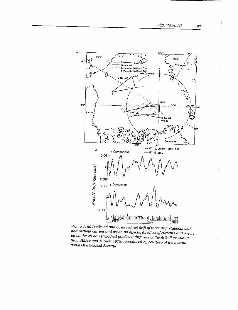
These characteristics are illustrated in Figure 1, which shows

short-term and long-term drift rates using a linear ice drift model.

As can be seen, including current effects has only a minor effect on

short-term variations. In examining cumulative drift over several

years, however, significant differences occur if currents and oceantilt are neglected. Basically, while smaller, current effects are

steady. On the other hand, wind effects, while large, tend to fluctu-

ate out over a long time period, leaving a smaller constant value.

W.D._i_bler,IIl 109

t20" 90"

,8o- _ _-_-- oh,,,-, c_,_)' L,.. us.sR /r.., _

; " "_ i/ - - - S;m.lot,dW.hout"n. .:,.., / ,,-- _ - "......... $imuloled Without Tilt %__._ /

J t t ./" _ "'"_. /t_lO I I

,50. , _ .-" ...--_ " _ _oo ,_o_..!3o"

'T3 ,_

90" 60"

b _ Wind, current ond tilt

r x Component --- Wind only

o£

£_ -006 _

0 06 y Component c

0 - I ,.,

i

-0 06-

Figure 1. (a) Predicted and observed net drift of three drift stations, with

and without current and ocean tilt effects; (b) effect of currents and ocean

tilt on the 25-day smoothed predicted drift rate of the Arlis II ice island

(from Hibler and Tucker, 1979; reproduced by courtesy of the Interna-tional GlaciologicaI Society).

; 110 Modeling the Earth System

=_

:5

Sea Ice Rheology

Sea ice motion results from a balance of forces that include wind

and water drag, sea surface tilt, and Ice interaction. The latter Is a

consequence of the large-scale mechanical properties of sea lcewhich include shear and compressive strengths but little tensile

resistance.In many cases the net effect of the ice interaction is to cause a

force opposing the wind stress roughly in the manner shown in Fig-

ure 2. As a consequence, to achieve the same ice velocity under

these circumstances, a larger wind stress more nearly parallel to the

ice velocity is required. This feature Is consistent with observations

by Thorndike and Colony (1982), which show ice motion to be very

highly correlated with geostrophlc winds, with the Ice drift rate

decreasing somewhat in winter for the same geostrophic wind. How-

ever, examination of drift statistics shows higher winds producing

an almost discontinuous shear near the coast. Moreover, observa-

tions show that while ice drift against the shore increases the ice

thickness, the buildup is not unlimited.

As noted by Hibler (1979), both of these characteristics of discon-

tinuous ice drift and a limit on near-shore ice buildup may be

explained by nonlinear plastic ice rheologies. These rheologies have

yield stresses that are relatively independent of strain rate. Hencefar from shore, even though the ice is interacting strongly, there

may be very low stress gradients since the stresses are relatively

Coriolis

_ Ice Velocity Water Drag

0.10 m s-1, Internal Ice Force

0.05 N rn-2I I

Fk3ure 2. An estimate of the force balance on sea lce for winter condi-tions based on wind and water stress measurements {from Hunkins,

1975). In this balance the force due to _nternal ice stress ts deter-

mined as a res_ual and the dashed line shows the lce veloci_.

W.D. 9_bler, HI 11 i

constant. Also this fixed yield stress will cause a discontinuous slip-

page at coastal points and prevent the Ice from building up without

bound. Without such a nonlinear rheology it is very difficult toobtain these features.

For climatic purposes probably the most important feature of the

ice Interaction is some type of resistance to Ice buildup that does

not drastically affect the ice drift. While this can be accomplished by

a nonlinear plastic rheology including a shear strength, reasonable

results may also be obtained by considering the ice to have only

resistance to compression and no resistance to dilation or shearing.

This "cavitating fluid" model has been compared by Flato and Hibler

(1990) to a more complete plastic rheology with good success. The

ice Interaction term for the cavitating fluid model ls characterized bythe following stress tensor:

alj = -P 8Ij (1}

where (_ij represents the i and j components of the two-dimensional

Cartesian stress tensor, P is Ice pressure, and 8ij is the Kroneckerdelta vehicle ls equal to 1 if i = j and 0 otherwise.

This rheology can be simulated using the viscous-plastic scheme

of Hibler (1979) or an iterattve method, in which the free drift veloc-

ity field ls calculated (I.e., by a simple analytic solution of the

momentum equation neglecting the Ice interaction term) and then

this estimated field is corrected in an lterative manner to account

for the compressive strength of ice. This correction can be accom-

plished by adding a small outward velocity component to each com-

putational grid cell such that after correction all convergence Is

removed. After a number of interactions all convergence will he

removed from the velocity field, simulating an Incompressible ice

cover. This correction procedure can also be formulated in terms of

an internal Ice pressure field, allowing specification of a failure

strength beyond which plastic flow ensues. A particularly simple

approximate solution to the cavitating fluid applicable to climate

modeling was presented earlier by Flato and Hibler (1990).

The appropriate yield stress depends on how one is characterizingthe Ice thickness distribution as discussed below. However, if one ls

using a simple two-level sea Ice model where H is the mean thick-

ness and A is the compactness (i.e., fraction of area covered by ice),

a reasonable yield stress P is given by

P = P*He-K(1-A) (2)

where K is 20, P* is a fixed strength constant (say 2.75 x 104 N/m2),

and e Is the exponential function. This strength formulation was

originally proposed by Hibler (1979) and has been utilized by Flato


-- 9 "/'

_Z_ ...... l/Ill'" _t.'/I l'" "_t. . .liitiv_.._ti/ . ; -

ti ",'/¢ilZl_''''' I. " •

• ,,,;_::' ...........

±:

j_

' ,r/l,,

- 1% .... _/1/it/i _...."

.5]_ .... iiiii ...... _ ,," _.i".i ' , -'_l/ltii_" "''I_..I'.'.*. " - " -

_' ,, ,, 2:

,% .,,,p/ ,¢r_ _ _ ; : :

, -.-

d _) ) "i

. .111: .:,. . <---.%: t <,.__,_)..,-'d"_"_r,, ,,1_.. ;':-

i ;,qm_t_¢ "t .':.

Figure 3. Average ice velocity fields calculated using forcing from March 1983: (a) free drift,

(b) incompressible cavitating fluid, (c) cavttattng fluid model with realistic compressive strength,

(d) viscous-plastic, elliptical yield curve model with shear and compressive strength.

==

:=

_=

and Hibler (1990, in press). This procedure is easily extended to

spherical coordinates as discussed by Flato and Hibler (in press).

An example of the use of the cavitating fluid model is shown in

Figure 3, where we have applied the cavitating fluid correction to thefree drift velocity field shown in Figure 3a. Two types of corrections

are applied: In Figure 3b a totally incompressible sea ice drift field isshown, while in 3c we have assumed a constant 3-m-thick ice every-where with a 2% fraction of open water. This, together with a yield

strength constant P* of 2.75 x 104 N/m 2, gives a maximum allow-able two-dimensional pressure of 5.53 × 10 4 N/m. As can be seen,

W.D. Hibler, III 11

-including a maximum yield pressure modifies the velocity field

somewhat Inasmuch as some convergence is allowed. The main

characteristic of both fields, however, is that the cavitating fluid

approximation does not damp out the Ice velocity field but rathersimply modifies it to prevent convergence.

A more complete sea ice rheology, the viscous-plastic elliptical

yield curve rheology, was presented by Hibler (1979). In this scheme

plastic failure and rate-Independent flow are assumed when the

stresses reach the yield curve values represented by an ellipse in

principal stress space. Here the compressive strength is given by the

length of the ellipse while the shear strength is given by its width.

Stress states inside the yield curve correspond to slow viscous creep

deformation. This model has been widely used and produces realis-

tic thickness and velocity patterns; however, its relative complexityand the dramatic slowdown in ice drift it produces when the wind

fields are temporally smoothed (Flato and Hibler, 1990) make it

somewhat less desirable for long-term climate studies. As a compar-ison, the velocity field calculated using this model with a constant

ice strength of 5.53 x 104 N/m Is shown in Figure 3d. Readilyapparent here is the less robust velocity field that results from the

increased resistance afforded by the shear strength. For a more

complete comparison of a variety of plastic rheologies for the Arctic

Basin, the interested reader is referred to Ipp et al. (in press), where

a variety of nonlinear rheologies are compared, including a more

exact solution to the cavitating fluid than presented above. It should

be noted that the approximate solution discussed here compares

very closely with exact, but less computattonally efficient, solution

methods (see, e.g., Flato and Hibler, In press).

It should be emphasized that the main reason for using some

model such as the cavitating fluid in Ice drift is to ensure that real-

istic ice transport occurs. When ice forms, heat is transferred to the

atmosphere (i.e., by the latent heat of fusion). When the ice melts

later at a different location, it absorbs this latent heat. Conse-

quently, In some sense, the net effect of ice transport is to transfer

heat from one location in the atmosphere to a different location. Ice

transport effects are even more pronounced for the oceanic circula-

tion in that where the Ice freezes, most of the salt is expelled into

the ocean. The Ice is then transported to a different location, where

it melts and produces a surface fresh water flux. These flux imbal-

ances play a critical role in the salt budget and circulation of the

Arctic Basin and may affect the global-scale ocean circulation by

producing fluctuations in effective surface precipitation in the North

Atlantic. Because of such considerations, climate studies must

include ice motion as well as ice thermodynamics.

L


=

Ice Thickness Distribution

A key coupling between sea Ice thermodynamics and ice dynam-

ics is the ice thickness distribution. Ice thickness ls an Important

factor in controlling deformation, which causes pressure ridging and

creates open water. When combined with ice transport, these factors

change the spatial and temporal growth patterns of the sea Ice and,

when coupled with mechanical properties of ice, can modify its

response to climatic change.Many features of the thickness distribution may be approximated

by a two-level sea Ice model (Hibler, 1979) where the ice thicknessdistribution is approximated by two categories: thick and thin. In

this two-level approach the ice cover is broken down into an area A

(often called the compactness), which is covered by ice with mean

thickness H, and a remaining area 1 - A, which is covered by thin

Ice, which, for computational convenience, is always taken to be of

zero thickness (i.e., open water).

For the mean thickness H and compactness A the following conti-

nuity equations are used:

3H/3t = -3(uH)/3x - 3(vH)/3y + Sh (3)

3A/3t : -3( uA )/3x - 3( vA )/Oy + S A (4)

where A < 1, u ls the x component of the ice velocity vector, v the y

component of the Ice velocity vector, and Sh and SA are thermody-

namic terms and are described in Hibler (1979).

The thermodynamic terms in Equations (3) and (4) represent the

total ice growth (Sh) and the rate at which lee-covered area is cre-

ated by melting or freezing (SA). The parameterization of the S A term

Is particularly difficult to do precisely within the two-level model and

generally represents one of the weaknesses of the model.To allow this model to be integrated over a seasonal cycle, it is

necessary to include some type of oceanic boundary layer or ocean

model. The simplest approach (used for example by Hibler and

Walsh, 1982) is to include a motionless fixed depth mixed layer

(usually 30 m In depth). With this model, any heat remaining after

all the ice ls melted ls used to warm the mixed layer above freezing.

Under ice growth conditions, on the other hand, the mixed layer is

cooled to freezing before the Ice forms. Another approach that treats

vertical penetrative convection processes much better Is to include

some type of one-dimensional mixed layer. Such an approach, usinga Kraus-Turner-like mixed layer, was carried out by Lemke et. al

(1990) for the Weddell Sea. Another approach Is to utilize a complete

oceanic circulation model which also allows lateral heat transport in

the ocean. The latter approach was used by Hibler and Bryan (1987)

W.D. J_bler, III 115

in a numerical investigation of the circulation of an ice-covered Arc-

tic Ocean. In this study, a two-level dynamic-thermodynamic sea ice

model was coupled to a fixed-level baroclinic ocean circulation

model. In this ice-ocean model the upper level was taken to be 30 m

thick and, as in the motionless case, was not allowed to drop below

freezing if ice was present. Inclusion of some type of penetrative con-

vection in a similar ice-ocean circulation model is an item of highpriority for future research and is presently being pursued.

A more precise theory of ice thickness distribution may be formu-

lated by postulating an areal ice thickness distribution function and

developing equations for the dynamic and thermodynamic evolution of

this distribution. In this case, a probability density g(H)dH is defined

to be the fraction of area (in a region centered at position x at time t)

covered by ice with thickness between H and H + dH. This distribu-

tion evolves In response to deformation, advection, growth, and decay.

Neglecting lateral melting effects, Thorndike et al. (1975) derived the

following governing equation for the thickness distribution:

_g{H} + V • [u_g(H}] +_t

_[fgg(H)]

_H = _ (5)

where u is the vector ice velocity with x and y components u and v,

V is the gradient operator, fg is the vertical growth (or decay) rate of

ice of thickness H, and _ is a redistribution function (depending on

H and g) that describes the creation of open water and the transfer

of ice from one thickness to another by rafting and ridging. Except

for the last term on the left-hand side and _ on the right-hand side,

Equation (5) is a normal continuity equation for g(H). The last term

on the left-hand side can also be considered a continuity require-ment in thickness space since it represents a transfer of ice from

one thickness category to another by the growth rates. An important

feature of this theory is that it presents an "Eulerlan" description in

thickness space. In particular, growth occurs by rearranging the rel-

ative areal magnitudes of different thickness categories.

This multilevel ice thickness distribution theory represents a very

precise way of handling the thermodynamic evolution of a contin-

uum composed of a number of ice thicknesses. However, the price

paid for this precision is the introduction of a complex mechanical

redistributor. In particular, to describe the redistribution one must

specify what portion of the ice distribution is removed by ridging,how the ridged ice is redistributed over the thick end of the thick-

ness distribution, and how much ridging and open water creation

occur for an arbitrary two-dimensional strain field, including shear-

ing as well as convergence or divergence. In selecting a redistributor

F

!


|

I_

Z

i]Z

Z-

=

7

±

= =

one can be guided by the conservation conditions that V renormal-

Izes the g distribution to unity due to changes In area and that

does not create or destroy ice but merely changes its distribution.

An additional consistency condition can be imposed if one asserts

that all the energy lost in deformation goes Into pressure ridging

and that the energy dissipated In pressure ridges is proportional to

the gravitational energy.A redistribution function that satisfies these constraints may be

constructed (for an explicit form see Hibler, 1980) by allowing open

water to be created under divergence and ridging to occur under

convergence. Within this formalism ridging occurs by the transfer of

thin ice to thicker categories, assuming a certain amount of ridging

and hence open water created under pure shear or more generally

under an arbitrary deformation state. This "energetic consistency"

condition will affect the thermodynamic growth via open water frac-

tions and hence the total Ice created.

The main relevance of the variable thickness distribution to cli-

mate modeling is its more precise treatment of the growth of ice. A

comparison of the two-level and multilevel approaches to modeling

the dynamic-thermodynamic evolution of an Ice cover will be pre-

sented below. However, here we note that the Ice thickness is con-

siderably greater with the multilevel model due to its more realistic

treatment of the thickness distribution.

Sea Ice Thermodynamic Models

Sea Ice grows and decays in response to long- and shortwave

radiation forcing, to air temperature and humidity via turbulent

sensible and latent heat exchanges, and to heat conduction through

the Ice. The heat conduction is significantly affected by the amount

of snow cover on the ice and by the brine remaining in the ice after

it has frozen. These internal brine pockets cause the thermody-

namic characteristics of sea ice to be very much different than those

of fresh water ice of the same thickness.

Many features of the thermal processes responsible for sea ice

growth and decay can be identified from semiemplrical studies of ice

breakup and formation of relatively motionless lake Ice and sea ice

(e.g., Langleben, 1971, 1972; Zubov, 1943). Overall, the two domi-

nant components of the surface heat budget relevant to sea ice

growth and freezing are the shortwave radiation during melting con-ditions and sensible and radiative heat losses during freezing.

Observations of fast Ice (relatively motionless Ice attached to land) at

the border of the Arctic Ocean Indicate that once the Initial stages of

breakup (snow cover melt and formation of melt ponds) have

W.D. Hibler, III 117

passed, the remaining decay of a stationary ice cover is almost

entirely due to the shortwave radiation incident on the ice surface

(Langleben, 1972). However, at the initial stages of breakup and

decay, the sensible heat flux plays an important role (when the air

temperature rises to ~ 0°C) in causing rapid melting of the surface

snow cover. This melting forms melt ponds (Langleben, 1971), which

reduce the albedo and greatly enhance the rate of ice melt. After

only a few weeks, drainage canals and vertical melt holes develop,

and the characteristic appearance of a summer ice cover evolves,

with melt ponds and surrounding smooth hummocks. Once these

melt ponds have formed, the remaining decay is dominated by theradiation absorbed by open water.

As is clear from this discussion, the decay of sea Ice in nature is

rather critically affected by the amount of open water, which,

because of its low albedo, can absorb much more radiation than the

Ice. On motionless ice sheets, the open water is present only

through melt ponds or holes. However, In an actual dynamic vari-

able-thickness ice cover, as occurs almost everywhere in the polar

regions, the growth and decay of sea ice can be substantiallyaffected by spatial thickness variations. Perhaps the most obvious

example is the effect of open water on the adjacent pack ice. Duringmelting conditions the radiation absorbed by leads can contribute to

lateral melting by ablation at the edges of ice floes.

A number of sea Ice thermodynamic models have been used in

the past, ranging from the simple empirical models of Zubov (1943)

and Anderson (1961) to complex numerical models that compute

the surface heat budget (Parkinson and Washington, 1979) and the

conduction through an inhomogeneous Ice sheet (Maykut andUntersteiner, 1971).

Equilibrium Thermodynamic Models

While it is possible to construct simpler thermodynamic models

that capture the essence of sea ice growth and decay (see

Thorndike, this volume), what is usually done in climate modeling is

to make use of an equilibrium ice/snow system in conjunction with

a complete surface heat budget. One can solve this system itera-

tively and come up with an ice growth rate. The basic idea is illus-

trated in Figure 4, In which the steady state temperature profile is

shown. Assuming no melting at the snow Ice interface, the amount

of heat going through this interface must be the same In the snowand the Ice so that

(6)

E

Z


E

5

z

5_

H s

TSnow

'y(TB-T o) Ti

ice

I FW

Figure 4. Sketch of combined snow and ice system used in equl-librium thermodynamic sea ice model. F w is oceanic heat flux;

other terms are defined in the text.

where Ti is the temperature of the ice at the snow-ice interface, T o is

the surface temperature of the snow, T B Is the water temperature, Kl

and Ks are the thermal conductivities of Ice and snow, and H i and H s

are the thicknesses of the Ice and snow.

This equation allows us to solve for T l in terms of T B and T 0. Sub-

stituting the resulting expression into the conductive flux through

the ice, we obtain

(Ti - TO)_s = T(TB - TO){71

=_

_CiKs is the effective conductivity.where y - [KsH i + KiHs ]

The complete surface heat budget equation, with a sign convec-

tion such that fluxes into the surface are considered positive, then

becomes

(1-ct)F s + FI + DlVg (Ta - TO)+ D2Vg[qa (Ta)- qs (T0)]- (81

D3T0 4 + (T)(TB - TO) = 0

where a is the surface albedo, Ta is the air temperature, T is the

effective conductivity, Vg is the wind speed, qa Is the specific humid-

ity of the air, qs is the specific humidity of the ice surface, and F s

W.D. Hibler, Ill 119

and F 1 are the incoming shortwave and longwave radiation terms.

The constants D 1 and D 2 are bulk sensible and latent heat transfer

coefficients, and D a is the Stefan-Boltzmann constant times the sur-

face emissivity. The equation is usually solved iteratively (see, e.g.,

Appendix B of Hibler, 1980, for details and numerical values of vari-

ous constants) for the ice surface temperature. The conduction of

heat through the Ice is used to estimate ice growth using

Y(Tb - T0)+F w =pl HdH1at (9)

where F w is the oceanic heat flux, Pi ls the Ice density, H l ls the Ice

thickness, and dHl/dt is the rate of change of ice thickness. When

the calculated surface temperature of the ice is above melting, it is

then set equal to melting, and the imbalance of surface flux is usedto melt ice.

Effect of Internal Brine Pockets and Snow Cover

Apart from the absence of dynamics, the global thermodynamic

models mentioned above are still somewhat simplified in nature, the

main simplification being that no internal melting due to brine

pockets in the Ice has been considered. In particular, in sea ice the

density, specific heat, and thermal conductivity are all functions of

salinity and temperature (the dependence on temperature is indi-

rectly also due to the salinity}. These dependencies are caused by

salt trapped in brine pockets that are in phase equilibrium with the

surrounding ice. The equilibrium is maintained by volume changesin the brine pockets. A rise in temperature causes the ice surround-

Ing the pocket to melt, diluting the brine and raising its freezingpoint to the new temperature. Because of the latent heat involved in

this Internal melting, the brine pockets act as a thermal reservoir,

retarding the heating and cooling of the ice. Since the brine has a

smaller conductivity and a greater specific heat than the lce, these

parameters change with temperature.

Maykut and Untersteiner {1971} developed a time-dependent

thermodynamic model for level multlyear sea ice and carried out a

variety of calculations that yielded considerable insight into the

growth and decay of sea ice. A simplified model that reproduced

most of the Maykut-Untersteiner results was proposed by Semtner

(1976}. The Semtner model assumed that sea ice could be repre-

sented as a matrix of brine pockets surrounded by ice where melting

can be accomplished internally by enlarging the brine pockets

rather than externally by decreasing the thickness. As a conse-

quence, for the same forcing sea ice can have a substantially greaterequilibrium thickness than fresh water ice.

!=


!

|

Based on this "brine damping" concept, Semtner (1976) proposed

a simple model in which the snow and ice conductivities were fixed.

In this model the salinity profile does not have to be specified. To

account for internal melting, an amount of penetrating radiation

was stored in a heat reservoir without causing ablation. Energy from

this reservoir was used to keep the temperature near the top of the

"ice from dropping below freezing in the fall. Using this simplified

model, Semtner was able to reproduce many aspects of Maykut and

Untersteiner's model results within a few percent.

For an even simpler diagnostic model, Semtner proposed that a

portion of the penetrating radiation I o be reflected away. The

remainder of I o was applied as a surface energy flux. In addition, to

compensate for the lack of internal melting, the conductivity wasincreased to allow greater winter freezing. In the simplest model, lin-

ear equilibrium temperature gradients are assumed in both the

snow and ice. Since no heat is lost at the snow-ice interface, the

heat flux is uniform in both snow and ice.

The results of Semtner's prognostic and diagnostic models are

compared to Maykut and Untersteiner's results in Figure 5. This fig-

ure also shows the importance of the assumed penetration of radia-

tion which causes internal melting. By allowing no radiation to pen-

etrate, the internal melting is mitigated and the radiation instead is

used to melt the ice, causing a reduced thickness. Note that while

the 0-1ayer diagnostic model reproduces the mean thickness well,

the amplitude and phase of the seasonal variation of thickness are

somewhat different from those of the 3-1ayer prognostic model. This

simplest diagnostic model has taken on special significance for

numerical simulations of sea ice because almost continual ridging

and deformation make it difficult to record the thermal history of a

fixed ice thickness. Selected thermodynamic-only simulations using

this model will be discussed in the next section.

Finally, because of the problems with an excessive seasonal cycle

in the simplest Semtner model, it may be useful to employ some

type of brine damping in sea ice models that are used in climatestudies. However, the difficulty here is that when a full dynamic

model is used, the advection of ice makes it difficult to record the

internal temperature characteristics of the ice. An approach that

improves the summer thermodynamic response of the ice cover is to

include a brine pocket heat storage term in an equilibrium one-level

model. Such an approach was carried out by Flato (1991) in a

numerical investigation of a variable-thickness sea ice model. While

his approach does not take into account the heat capacity of the ice,

it does create a much more realistic summer cycle in that it retards

spring melting and fall freezing.


3.50

3.00

2.50

2.00I I I I I I I I I I I I

J F M A M d J A S O N DMonth

Figure 5. Annual thickness cycles of three thermodynamic sea ice models forthe cases of O and 17% penetrating radiation. Solid line, Maykut-Untersteiner

model; dashed line, Semtner 3-1ayer model; dotted line, Seminer O-layer model.

The role of snow cover In modifying the thermodynamic growth of

sea Ice was also investigated by Maykut and Untersteiner (1971)and Semtner (1976). The thermal conductivity of snow is consider-

ably less than that of ice; however, the albedo of snow Is much

higher than that of ice. Lower conductivity Implies less ice growth,

whereas higher albedo Implies less summer melt. These conflictingprocesses combine to produce little change in mean annual Ice

thickness for snowfall rates less than about 80 cm/yr. Since this ls

much higher than the snowfall rate for most of the Arctic, snow

cover can be expected to have little effect on the amount and distrib-

ution of sea Ice. This notion Is confirmed by recent dynamic-thermo-

dynamic simulations with a multilevel sea ice model that included

the effect of snowfall (Flato, 1991).

Model Simulations of Arctic Sea Ice

Sea ice in climate models has generally been included simply as a !

motionless sheet, in some cases using a thermodynamic growthmodel to calculate the surface temperature and ice thickness. As


=

]

£

%

Z

]

discussed above, neglecting ice dynamics not only removes the lat-

eral heat and salt transport capabilities of the ice pack, it also leads

to unrealistic spatial patterns of thickness buildup and air-sea heatfluxes. In this section we will discuss some numerical model results

to illustrate a few of these effects. In particular we will compare free

drift (no ice interaction), the cavitating fluid rheology, and the ellipti-

cal yield curve, viscous-plastic rheology in simulations employingclimatological wind and thermodynamic forcing (Flato and Hibler,

1990). For comparison we will also show the result of a thermody-

namics-only simulation in which the ice cover is assumed to be a

motionless, unbroken sheet.

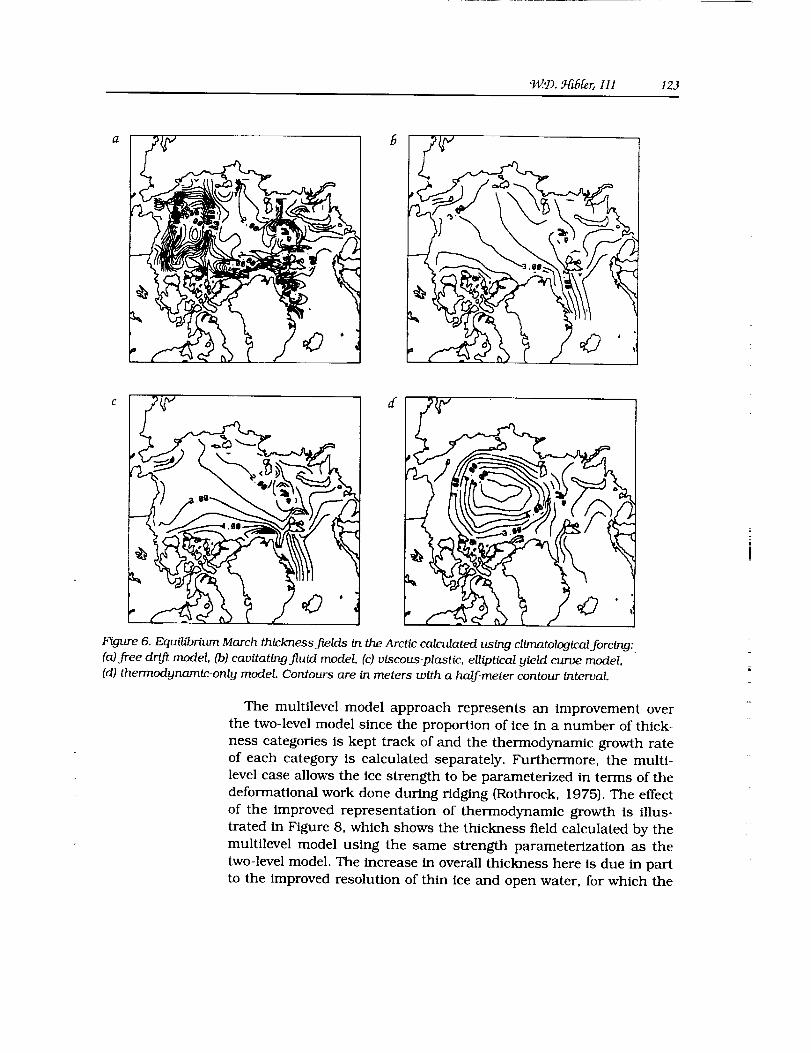
Perhaps the most illustrative comparison of these simulations is

provided by the seasonal equilibrium thickness contours (Figure 6)shown here for the end of March. The lack of ice interaction in the

free drift case leads to unreasonable thickness buildup near the

coasts after only a couple of months and is thus clearly undesirable

for climate studies. Both the cavitating fluid and viscous-plastic

models produce thickness buildup patterns which are roughly simi-lar to observations (e.g., Bourke and Garrett, 1987), with the thick-

est ice (4-6 m) off the Canadian Archipelago and North Greenland

coast. The similarity here reinforces the notion that, to lowest order,

the role of ice interaction is to prevent excessive convergence when

ice is driven against a coast. Shear strength in the viscous-plastic

case acts primarily to slow the ice drift and impede outflow through

the Fram Strait (Flato and Hibler, 1990), although it does modify the

thickness buildup pattern somewhat. We might note, however, that

including shear strength in the ice cover modifies the curl of the

wind stress applied to the ocean and thus influences the barotropicocean circulation, a modification which may be important in long-

term ice-ocean simulations. It is also interesting that the net ice

growth patterns (contours of net ice growth at a point over a year)are almost unaffected by shear strength in the ice cover (Figure 7),

and, since net growth corresponds to a net source of salt at the

ocean surface, the baroclinic ocean circulation should be impacted

little. In addition to the unrealistic thickness patterns, it is this lastissue which makes the thermodynamics-only model unsuitable for

long-term climate studies with a coupled ice-ocean model. The prob-lem here is that in a thermodynamics-only model the ice grows and

melts in place, and hence, over an annual cycle, there is no net saltflux to the ocean. Atmospheric general circulation models can toler-

ate coupling to a thermodynamics-only sea ice model since the prin-

cipal bottom boundary condition is temperature; however; some

parameterization of leads is necessary if the fluxes of heat and water

vapor are to be at least crudely included.

'_.D. _YU_[er_III 123

f b!!

d

Figure 6. Equilibrium March thickness fields in the Arctic calculated using climatological forcing:(a) free drift model, (b) cavitating fluid model, (c) viscous-plastic, elliptical yield curve model,

(d) thermodynamic-only model. Contours are in meters with a half-meter contour interval.

The multilevel model approach represents an improvement over

the two-level model since the proportion of ice In a number of thick-

ness categories is kept track of and the thermodynamic growth rate

of each category Is calculated separately. Furthermore, the multi-

level case allows the ice strength to be parameterized in terms of the

deformational work done during ridging (Rothrock, 1975). The effect

of the improved representation of thermodynamic growth Is illus-

trated in Figure 8, which shows the thickness field calculated by the

multilevel model using the same strength parameterization as the

two-level model. The increase in overall thickness here ls due in part

to the improved resolution of thin ice and open water, for which the


©

Figure 7. Net annual ice growth flelds (in meters of ice per year)

calculated using climatological forclng: (a} vlscous-plastic, ellip-

tical yield curve model, (b) cavitating fluid model. The contour

interval is 0.25 m of ice per year.


ll

j

, , _iii ,e , _' t'(

! " EEA,,\ "X",-J

Figure 8. Equilibrium March thickness fields calculated using (a) climatological forcing.

together with (b) a multilevel sea ice model with two-level model strength parameterization.Contours are in meters with a half-meter contour interval.

growth rate Is very high, and redistribution from thin to thick Ice

representing the formation of ridges during deformation. It is likelythat the complexity and computational demands of the multilevel

model are unjustified for climate studies at this point, although a

simpler three- or four-level model (currently under development)

would be a significant improvement over the two-level scheme.

Sensitivity of Sea Ice Models to Climate Change

In this section we will demonstrate the sensitivity of the modeled

sea ice cover to changes in atmospheric forcing which might accom-pany changes In global climate. Aside from dramatic alterations in

atmospheric circulation patterns, the most significant impact on the

ice cover will likely be due to changes in air temperature and cloud

cover. An increase in air temperature results in greater sensible and

latent heat fluxes and incident longwave radiation, all of which

inhibit ice growth. An increase in the cloud cover, on the other

hand, reduces the incoming shortwave radiation while increasing

the longwave flux. These effects will be investigated here by examin-

ing several simulations of the Arctic ice cover using the two-level

dynamic-thermodynamic sea ice model with forcing fields coveringthe period 1981-83.

The four simulations we will discuss here are the standard or

unperturbed run, runs in which the cloud cover was increased or

decreased by 20%, and a run In which the air temperature was

increased by 1°C. Time series of total ice volume and ice extent (the


=

=

32000.0

28000.0

24000.0

"-", 20000.0

16000.0

12000.0

8000.0

4000.0

\ ,7/

_X\" -' II ,'-,%I_,'

l i

,/,'/_...,///I/i

i

/o

t ..: /

_L% / ,'

_I /

'_ i

0.0 I l I t t I 1 I n l I 1 I t I t I

0 6 12 18 24 30 36

Month

Figure 9. Total ice volume and ice extent (area enclosed by 15% compactness

contour) time series calculated using two-level viscous-plastic model and forcing

fields from 1981-83. Results are shown for (solid line) a standard simulation,

(dotted line) a case with cloud cover increased by 20%, (dashed line) a case

with cloud cover decreased by 2096, and (dot-dashed line) a case with a I°C

increase in air temperature.

area enclosed by the 15% compactness contour) are plotted in Fig-ure 9 and show the sensitivity to each of these changes. The

increase in total ice volume and summer ice extent in the increased

cloud cover case points out that the dominant role of clouds is to

control the incoming shortwave radiation--their contribution to

longwave radiation being secondary. It is also apparent from the

asymmetry of the response to increasing and decreasing the cloudcover that this effect is rather nonlinear. A significant decrease in

both ice volume and summer ice extent is seen to accompany a 1°C

rise in air temperature; in fact, the summer ice volume is reduced

by almost a third. An increase in air temperature of about 4°C (avalue obtained by Manabe and Stouffer, 1980, for a doubling of

CO2) is sufficient to almost eliminate the summer ice cover. What is

missing here, of course, is the feedback between the increase in

open water area and the amount of cloud cover. The increase in

open water area, not only in the peripheral seas but also in the

central pack, is illustrated by the August 1983 compactness fieldsfor the four simulations (Figure 10). A general increase in cloud


!d

Figure 10. Compactness fields calculated by the two-level model for August 1983: (a) standardsimulation, (b) 20% increase in cloud cover, (c) 20% decrease in cloud cover, (d) I°C increase in air

temperature.

cover would be expected in the warming case due to the increased

availability of water vapour from leads, and this, based on the

cloud sensitivity results, may counteract the effect of increased air

temperature.

We might note here that the ice edge location, particularly in the

eastern Arctic, is somewhat too far north in these simulations--a

shortcoming of the two-level model. The ice edge position is some-

what better in the multilevel model case; however, the sensitivity to

clouds and warming is about the same. We should also point out

here that the shape and interannual variability of the ice edge in the


Barents and Greenland seas is controlled primarily by upwelling of

heat from the ocean. To properly simulate the ice cover in this cli-

matically important region requires a coupled ice-ocean model

which not only provides realistic ocean currents (to properly repre-

sent the lateral transport of heat) but also includes a sufficiently

detailed parameterization of the vertical processes to bring the heat

from the deeper ocean to the surface at the correct location.

Concluding Remarks

Because of almost constant motion and deformation, the dynam-

Ics and thermodynamics of sea ice are intrinsically coupled. In addi-

tion, the Ice and ocean circulation are tied together by the freezing

and melting of ice, which causes salt and fresh water fluxes into the

ocean, and ice transport, which yields unbalanced fluxes. As a con-

sequence, understanding the response of the high latitudes to cli-

matic change requires considering the coupled ice-ocean system

(including ice interaction) in the polar regions. Results and theory

reviewed here have indicated the complexity of different thermody-

namic and dynamic effects and the role they can play in air-sea

interaction. This complexity makes it difficult to guess the correct

ad hoc treatment of sea ice to use in climate models. Instead, the

results emphasize the importance of including a more realistic treat-

ment of sea ice vis-_i-vis a fully coupled, ice interaction-based,

dynamic-thermodynamic sea ice model. These models at least con-

tain the main first-order aspects of the sea ice system, whereas simple

thermodynamics-only models clearly do not.

By coupling such models with treatments of the ocean, we may

obtain quantitative insights. It also appears that due to the variety

of complex dynamic processes, specifying ice fluxes and transport

for use in ocean circulation modeling will leave out many major

feedbacks that affect climatic change.

References

Anderson, D.L. 1961. Growth rate of sea ice. Journal of Glaciology 3,

1170-1172.

Bourke, R.H., and R.P. Garrett. 1987. Sea ice thickness distribution in the

Arctic Ocean. Cold Region Science and Technology 13, 259-280.

Flato, G.M. 1991. Numerical Investigation of the Dynamics of a Variable

Thickness Arctic Ice Cover. Ph.D. thesis, Thayer School of Engineer-

ing, Dartmouth College, Hanover, New Hampshire.

Flato, G.M., and W.D. Hibler, III. 1990. On a simple sea ice dynamics model

for climate studies. Annals of Glaciology 14, 72-77.

W.D. H_bler, Ill 129

Flato, G.M., and W.D. Hibler, Ill. On modeling pack ice as a cavitating fluid.

Journal of Physical Oceanography, in press.

Hibler, W.D., III. 1979. A dynamic thermodynamic sea ice model. Journal of

Physical Oceanography 9, 815-846.

Hibler, W.D., Ill. 1980. Modeling a variable thickness sea ice cover. Monthly

Weather Review 108, 1942-1973.

Hibler, W.D., Ill, and K. Bryan. 1987. Ocean circulation: Its effect on sea-

sonal sea ice simulations. Science 224, 489--492.

Hibler, W.D., III, and G.M. Flato. Sea ice models. In Climate Systems Model-

ing (K. Trenberth, ed.), Cambridge University Press, Cambridge,

England, in press.

Hibler, W.D., III, and W.B. Tucker. 1979. Some results from a linear viscous

model of the Arctic ice cover. Journal of Glaciology 4, 110.

Hibler, W.D., Ill, and J.E. Walsh. 1982. On modeling seasonal and interan-

nual fluctuations of arctic sea ice. Journal of Physical Oceanography

12, 1514-1523.

Hunkins, K. 1975. The oceanic boundary layer and stress beneath a drifting

ice floe. Journal of Geophysical Research 80, 3425--3433.

Ip, C.F., W.D. Hibler, Ill, and G.M. Flato. On the effect of rheology on sea-

sonal sea ice simulations. Annals of Glaciology, in press.

Langleben, M.P. 1971. Albedo of melting sea ice bottomside features in the

Denmark Strait. Journal of Geophysical Research 79, 4505-4511.

Langleben, M.P. 1972. Decay of an annual cover of sea ice. Journal of

Glaciology 11,337-344.

Lemke, P., W.B. Owens, and W.D. Hibler, III. 1990. A coupled sea Ice-mixed

layer-pycnocline model for the Weddell Sea. Journal of Geophysical

Research 95, 9513-9526.

Manabe, S., and R. Stouffer. 1980. Sensitivity of a global climate model to

an increase of CO 2 concentration in the atmosphere. Journal of

Geophysical Research 85, 5529-5554.

Maykut, G.A., and N. Untersteiner. 1971. Some results from a time depen-

dent, thermodynamic model of sea ice. Journal of Geophysical

Research 76, 1550-1575.

Parkinson, C.L., and W.M. Washington. 1979. A large-scale numerical

model of sea ice. Journal of Geophysical Research 84, 311-337.

Rothrock, D.A. 1975. The energetics of the plastic deformation of pack ice

by ridging. Journal of Geophysical Research 80, 4514--4519.

Semtner, A.J., Jr. 1976. A model for the thermodynamic growth of sea ice in

numerical investigations of climate. Journal of Physical Oceanogra-

phy 6, 379-389.


Thorndike, A.S., and R. Colony. 1982. Sea ice motion in response to

geostrophic winds. Journal of Geophysical Research 87, 5845-5852.

Thorndike, A.S., D.A. Rothrock, G.A. Maykut, and R. Colony. 1975. The

thickness distribution of sea ice. Journal of Geophysical Research

80, 4501--4513.

Zubov, N.N. 1943. Arctic Ice. Translation, National Technical Information

Service (AD426972), Washington, D.C., 491 pp.

mE

7

the role of sea ice dynamics in global climate change · the role of sea ice dynamics in global...

Documents