the role of the exchange rate in the economic growth
TRANSCRIPT
NBB WORKING PAPER No.9 - MAY 2000
THE ROLE OF THE EXCHANGE RATE IN ECONOMIC GROWTH:A EURO-ZONE PERSPECTIVE_______________________________
Ronald MacDonald(*)
(*) Department of Economics, University of Strathclyde, 100 Cathedral St, Glasgow, G4 OLN.
Conference1 5 0 t h a n n i v e r s a r y
NATIONAL BANK OF BELGIUM
WORKING PAPERS - RESEARCH SERIES
WORKING PAPER No.9 - MAY 2000
Editorial Director
Jan Smets, Member of the Board of Directors of the National Bank of Belgium
Statement of purpose:
The purpose of these working papers is to promote the circulation of research results (Research Series) and analyticalstudies (Documents Series) made within the National Bank of Belgium or presented by outside economists in seminars,conferences and colloquia organised by the Bank. The aim is thereby to provide a platform for discussion. The opinions arestrictly those of the authors and do not necessarily reflect the views of the National Bank of Belgium.
The Working Papers are available on the website of the Bank:http://www.nbb.be
Individual copies are also available on request to:NATIONAL BANK OF BELGIUMDocumentation Serviceboulevard de Berlaimont 14B - 1000 Brussels
Imprint: Responsibility according to the Belgian law: Jean Hilgers, Member of the Board of Directors, National Bank of Belgium.Copyright © National Bank of BelgiumReproduction for educational and non-commercial purposes is permitted provided that the source is acknowledged.ISSN: 1375-680X
NBB WORKING PAPER No.9 - MAY 2000
Abstract
In this paper we consider a range of topics which connect exchange rates to
the economic growth process. In particular, we first of all outline the basic properties of
exchange rates when they are flexible. One key feature of flexible exchange rates is that
they are highly volatile and such volatility may affect growth through the channels of trade
and investment. These channels are considered in some detail in this paper. We also
consider the links between sectoral and aggregate growth and the exchange rate, using
the Balassa-Samuelson and Houthakker-Magee-Krugman hypotheses. The main
conclusion of the paper is that the current exchange rate arrangements for the euro-zone
area, both internal and external, are likely to stimulate economic growth.
Editorial
On May 11-12, 2000 the National Bank of Belgium hosted a Conference on "How topromote economic growth in the euro area?". A number of papers presented at theconference is made available to a broader audience in the Working Papers series ofthe Bank. This volume contains the fifth of these papers. The other five papers wereissued as Working Paper 5-8 and 10.

WORKING PAPER No.9 - MAY 2000
NBB WORKING PAPER No.9 - MAY 2000
TABLE OF CONTENTS:
1. INTRODUCTION.........................................................................................................................1
2. SOME STYLISED FACTS ABOUT REAL AND NOMINAL EXCHANGE RATE
BEHAVIOUR...............................................................................................................................5
3. ESTIMATION METHODS - A DIVERSION ..............................................................................11
4. EXCHANGE RATE MODELS AND ECONOMIC GROWTH ...................................................12
5. EXCHANGE RATE REGIMES AND ECONOMIC GROWTH ..................................................16
6. THE GROWTH - EXCHANGE RATE LINK..............................................................................18
6.1 Decomposing the real exchange rate: Violations of the LOOP and the
Balassa-Samuelson hypothesis.....................................................................................19
6.2 The Houthakker-Magee-Krugman 45° Rule...................................................................26
7. THE EXCHANGE RATE - GROWTH LINK..............................................................................33
7.1 Exchange rates and international trade ........................................................................33
7.1.1 Theory ..................................................................................................................33
7.1.2 Evidence ..............................................................................................................39
7.2 Exchange Rates and Investment ...................................................................................44
8. CONCLUSIONS........................................................................................................................49
9. REFERENCES..........................................................................................................................52

WORKING PAPER No.9 - MAY 2000
WORKING PAPER No.9 - MAY 2000 1
1. INTRODUCTION
The role of the exchange rate in the economic growth process is not immediately apparent
from a cursory glance at the growth literature. Indeed, the idea that a financial price can
have real effects would at first blush perhaps seem to be a rather odd idea. However,
some clues to the likely effects of exchange rates on growth may be gleaned from the
behaviour of exchange rates when they are flexible. First, in a flexible exchange rate
regime there is a very close correlation between real and nominal exchange rates and it is
widely accepted, although not uncontroversial, that in the presence of sticky prices it is the
nominal exchange rate which drives the real exchange rate. Furthermore, once a real
exchange rate change occurs that change tends to be highly persistent or, indeed,
permanent. Another feature of exchange rates when they are flexible is that they tend to
be extremely volatile and such volatility has been argued to be excessive, in the sense that
there appears to be no corresponding volatility in the kinds of variables driving exchange
rates, such as relative money supplies and prices. What is the relationship between such
exchange rate behaviour and economic growth?
In my lecture today I am going to take the body of economic growth theory as given and
simply think of economic growth as driven by changes in the factor proportions, along the
lines of a standard growth accounting relationship. What effect does the exchange rate
have on these proportions? For the purposes of this lecture, it shall prove useful to
decompose growth into permanent, cyclical and transitory components as:
,yyy tCt
Ptt ε++=∆ (1)
where ty denotes the natural logarithm of national income, ? is the first difference
operator, and therefore ? ty represents the growth rate, pty and c
ty are the permanent and
cyclical components of national income and tε is a transitory term. The permanent
component may be thought of as related to long-run, or steady state, growth and the
cyclical element is the business cycle-related component. How can the exchange rate
influence pty and c
ty ? In this paper we distinguish between two potential exchange rate
effects: a level and a volatility effect. The level effect might occur when a country
experiences, say, a sustained appreciation of its nominal and real exchange rates, due to
a tight monetary policy. This could make part, or all, of the country's traded sector
WORKING PAPER No.9 - MAY 20002
unprofitable. The initial response of this exchange rate change may well be for firms
exposed to trade to reduce their labour inputs to the existing capital stock and this could
have a cyclical effect on growth. If the exchange rate misalignment was sufficiently
prolonged then parts of the tradable sector could simply disappear, as occurred in the UK
in the late 1970s and early 1980s. One could also imagine such a levels effect influencing
the decision to invest in new capital for the country experiencing the misalignment.
However, perhaps the main channel by which the exchange rate is thought to influence
economic growth is through the effect of exchange rate volatility on the profitability of
international trade and investment. Indeed, the unattractive implications of exchange rate
volatility for trade and investment has been argued to be one of the major weaknesses of
floating exchange rate regimes (see for example Group of Twenty Four (1985) and the
Group of Ten (1985)) and this certainly has been one of the driving forces for greater fixity
of exchange rates within Europe, and also is behind calls for greater fixity of the tripolar
three exchange rates - the euro, dollar and yen. Although it is sometimes argued that the
existence of capital markets, and in particular a well developed forward market, should
internalise the unpleasant consequences of exchange rate volatility, hedging is costly, and
sometimes prohibitively so. Furthermore, such markets are often incomplete, particularly
at horizons of greater than one year. We return to the issue of hedging below.
How important are the exchange rate effects discussed above likely to be for the
euro-zone area? This is one of the aspects of the growth - exchange rate relationship I
want to address in my lecture today. If we are prepared to think in terms of a causality
relationship, then this effect may be thought of as exchange rate movements causing
growth (positive or negative). There are two dimensions to this. First, there is the internal
dimension - to what extent have locking exchange rates within Europe squeezed out the
unpleasant consequences of exchange rate behaviour for intra-European trade and
investment? Some insight into this question may be gleaned from an examination of the
linkages that existed prior to the formation of the euro. Second, how important is this
effect likely to be for the euro-zone area vis-à-vis its external trading partners? Given that
the euro-zone as an entity is a relatively closed area in terms of international trade, it may
be thought that this external effect is likely to be relatively small.
There is, however, another causality link between growth and the exchange rate, which is
essentially the reverse of the above. Although there are various rationalisations for this
effect, one that I shall discuss in this paper is related to the time series properties of real
WORKING PAPER No.9 - MAY 2000 3
exchange rates. For example, and as I shall demonstrate below there is considerable
long-run, or secular, persistence in real exchange rates. What explains this persistence
and is the degree of persistence similar within and across monetary unions? Although
there are a number of potential candidates to explain the persistence of real exchange
rates there are two which are particularly pertinent to the topic of this lecture. One is the
socalled Balassa-Samuelson effect which posits that a country which has relatively high
productivity in its traded goods sector, compared to its non-traded goods sector, will have
an overvalued currency relative to its trading partner(s). Furthermore, if the productivity
growth in the home country's tradable sector is more favourable relative to its trading
partners over time, this will impart a secular appreciation into its real exchange rate.
Clearly, if this effect is significant it could have important policy implications for the internal
workings of a newly formed monetary union since it implies that with a fixed nominal
exchange rate the repercussions must be reflected in relative prices or inflation
differentials. Are such differentials likely to be sustainable? To what extent, then, is the
Balassa-Samuelson, effect important for the kinds of countries participating in EMU? An
alternative perspective on the persistent nature of real exchange rates may be found in
what I will refer to as the Houthakker-Magee-Krugman (HMK) hypothesis. This hypothesis
suggests that countries with different long term growth rates, relative to their trading
partners, or countries which face different elasticities of import and export demand, may
suffer secular changes in their real exchange rate. Again, the extent to which this
relationship does, or does not hold, for euro-zone countries may have important policy
implications.
A final spin on the growth-exchange rate link, which has been brought into sharp relief
recently by the sharp depreciation of the euro, is the effect of relative business cycle
growth on an exchange rate. A number of commentators have argued that the euro is
weak because aggregate growth in the euro-zone area is relatively slow; once growth in
the euro-zone catches up with US growth, the euro will start to appreciate. We briefly
discuss this linkage in section 4.
I am going to give my discussion of the growth - exchange rate topic an explicitly European
perspective by generating some new empirical results for key EU countries. For the
euro-zone area we may think of essentially two exchange rates: the internal and the
external. Prior to monetary union there was some flexibility in the nominal and real
exchange between European countries and there was much more flexibility in the external
nominal and real exchange rates vis-à-vis non-European countries, such as the US. The
WORKING PAPER No.9 - MAY 20004
advent of monetary union, of course, means that internal nominal rates are now rigidly
fixed within Europe, although internal real rates can vary, while the external value of both
the real and nominal euro have been flexible. Given that the euro-zone area is relatively
closed - trade and investment is predominantly amongst EU countries - it has been
suggested that the external flexibility of the euro is unlikely to have particularly large
implications for the euro-zone area. I attempt to get a feel for the likely effects of exchange
rate movements on euro-zone growth by constructing panel data sets consisting of the
currencies of countries which are currently full participants of EMU. These panel data sets
try to capture the effects of both internal and external exchange rate movements.
In sum, our approach to thinking about the growth - exchange rate relationship for the
euro-zone area essentially involves presenting a smorgasbord of topics which seem
relevant to this issue. In the next section we set the scene by presenting some stylised
facts about the behaviour of real and nominal exchange rates in a flexible rate regime.
Section 3 details the estimation methods used for our empirical results. We then go on in
Section 4 to look at what a selection of open economy macro-economic exchange rate
models have to say about exchange rate - growth linkages. In section 5 a brief of overview
of the effects of the exchange rate regime on economic growth from an historical
perspective is presented. In section 6 the relationship between growth and the exchange
rate is considered by examining the Balassa-Samuleson and Houthakker-MageeKrugman
hypotheses; some new empirical results are also presented in this section. In section 7 we
focus on the potential role of the exchange rate in creating economic growth through the
channels of investment and international trade. A concluding section gathers together the
various points made throughout the paper.
WORKING PAPER No.9 - MAY 2000 5
2. SOME STYLISED FACTS ABOUT REAL AND NOMINAL EXCHANGE RATE
BEHAVIOUR
Some insight into the topic of this lecture may be gleaned by asking the question: how do
exchange rates behave when they are flexible? There are a number of so-called sylised
facts relating to this question. First, when exchange rates are flexible they tend to be
highly volatile. This volatility is usually gauged in a number of ways: on an historical basis
when comparing the recent flexible rate experience with fixed, but adjustable, exchange
rate regimes, such as the Bretton Woods regime; exchange rates are volatile relative to
some measure of the expected exchange rate, such as the forward exchange rate or the
expectation implied by survey data. exchange rates are volatile relative to certain
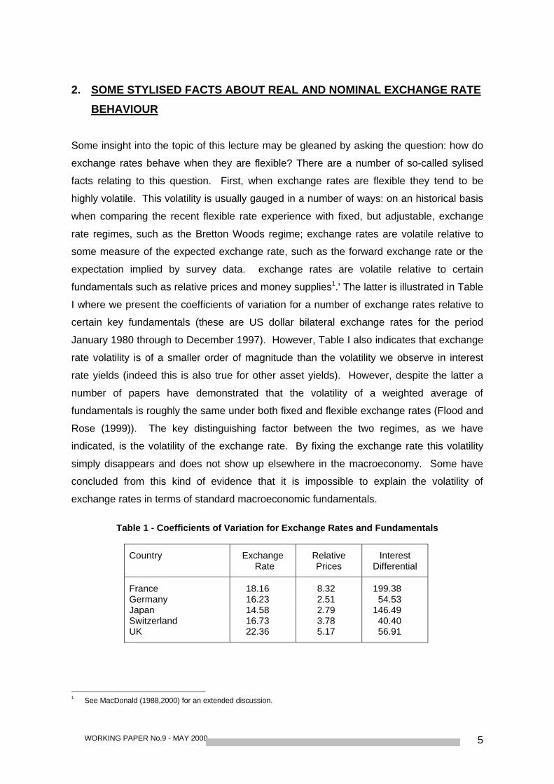
fundamentals such as relative prices and money supplies1.' The latter is illustrated in Table
I where we present the coefficients of variation for a number of exchange rates relative to
certain key fundamentals (these are US dollar bilateral exchange rates for the period
January 1980 through to December 1997). However, Table I also indicates that exchange
rate volatility is of a smaller order of magnitude than the volatility we observe in interest
rate yields (indeed this is also true for other asset yields). However, despite the latter a
number of papers have demonstrated that the volatility of a weighted average of
fundamentals is roughly the same under both fixed and flexible exchange rates (Flood and
Rose (1999)). The key distinguishing factor between the two regimes, as we have
indicated, is the volatility of the exchange rate. By fixing the exchange rate this volatility
simply disappears and does not show up elsewhere in the macroeconomy. Some have
concluded from this kind of evidence that it is impossible to explain the volatility of
exchange rates in terms of standard macroeconomic fundamentals.
Table 1 - Coefficients of Variation for Exchange Rates and Fundamentals
Country ExchangeRate
RelativePrices
InterestDifferential
France 18.16 8.32 199.38Germany 16.23 2.51 54.53Japan 14.58 2.79 146.49Switzerland 16.73 3.78 40.40UK 22.36 5.17 56.91
1 See MacDonald (1988,2000) for an extended discussion.
WORKING PAPER No.9 - MAY 20006
In order to get a feel for the relative volatility of currencies, as opposed to their volatility
relative to fundamentals, we present in Table 2 coefficients of variation for a group of
European currencies, including those who have irrevocably locked their exchange rates
within Europe. The rates are defined with respect to three numeraire currencies - the DNI,
the Yen and the US Dollar. These show that the volatility of the US and dollar rates are
about the same order of magnitude, but that the ERM effect has attenuated the volatility of
the DM-based currencies to around one-half of that observed in the other rates.
Furthermore, the volatility of all three rates is sample-specific, with the period of the 80's, a
period when the convergence process was perhaps at its greatest in Europe, exhibiting the
smallest volatility.
A second stylised fact about exchange rates is that there is a very close correspondence
between real and nominal exchange rates. Although the interpretation of what causes this
volatility is controversial, we would argue that it is the nominal exchange rate which drives
the real exchange rate. Clearly such real changes could impact on the profitability of the
tradable sector and this could affect growth in the medium run and also, perhaps, in the
longer run. The close correlation between real and nominal exchange rates is illustrated in
Figure 12 and also in Table 2 where we note that the relative nominal volatility of
currencies discussed above seems to get transferred into roughly equivalent real volatility.
A third stylised fact about the behaviour of real exchange rates is that they are highly
persistent. Evidence of such persistence may be obtained from the recent literature on
Purchasing Power Parity (PPP)3.' For example, single currency univariate unit root tests
suggest that real exchange rates are effectively non-stationary, or to the extent that they
do exhibit any mean reversion it is incredibly slow. In Table 3 we present some univariate
unit root statistics to illustrate this persistence for the currencies examined in this paper.
Three sample periods are considered: a full sample, 1980, quarter 1, to 1998, quarter 4
and two sub-samples within the full sample (1980,1 to 1989,2 and 1989,3 to 1998,4).
These results indicate an inability to reject the null for any sample period for the DM and
US dollar based currencies, although we note that 5 rejections for the yen based
currencies occur in the full sample. These kind of results can usually be overturned by
increasing the span of the data. Here we accomplish this by stacking the three sets of real
exchange rates into panels and constructing Levin and Lin (1994) panel unit root t-tests
and adjusted t-tests (adjt), along with the implied degree of quarterly adjustment ( )δ .
2 The correlation between real and nominal exchange rates is approximately 0.9.3 See, for example, MacDonald (1995,2000).
WORKING PAPER No.9 - MAY 2000 7
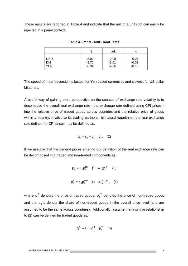
These results are reported in Table 4 and indicate that the null of a unit root can easily be
rejected in a panel context.
Table 4 - Panel - Unit - Root Tests
t adjt d
USD -5.02 -2.28 -0.05DM -5.70 -2.01 -0.08YEN -8.34 -4.76 -0.13
The speed of mean reversion is fastest for Yen based currencies and slowest for US dollar
bilaterals.
A useful way of gaining extra perspective on the sources of exchange rate volatility is to
decompose the overall real exchange rate - the exchange rate defined using CPI prices -
into the relative price of traded goods across countries and the relative price of goods
within a country, relative to its trading partners. In natural logarithms, the real exchange
rate defined for CPI prices may be defined as:
.ppsq *tttt +−≡ (2)
If we assume that the general prices entering our definition of the real exchange rate can
be decomposed into traded and non-traded components as:
,p)1(pp Ttt
NTttt α−+α= (3)
,p)1(pp *Ttt
*NTtt
*t α−+α= (4)
where Ttp denotes the price of traded goods, NT
tp denotes the price of non-traded goods
and the tα 's denote the share of non-traded goods in the overall price level (and are
assumed to be the same across countries). Additionally, assume that a similar relationship
to (2) can be defined for traded goods as:
*Tt
Ttt
Tt ppsq +−= (5)
WORKING PAPER No.9 - MAY 20008
By substituting (3), (4) and (5) in (2) the following expression may be obtained:
[ ],)p(p)p(pqq Tt
NTt
*Tt
*NTt
Ttt −α−−α+= (6)
,qqq NT,Tt
Ttt += (7)
( ) ( )[ ]Tt
NTt
*Tt
*NTt
T,NTt ppppq −−−α= (8)
The first term in (6), Ttq , represents the law of one price (LOOP), or violations of the
LOOP, while the second term, T,NTtq represents the so relative price ratio and is usually
associated with the Balassa-Samuelson effect, considered in some detail in section 6,
although it can also be driven by demand side influences, such as the effect of government
expenditure or preference shifts. On the assumption that the LOOP holds, expression (6)
predicts that if the home country has a relatively high internal price ratio it will have an
appreciated real exchange rate defined using overall prices. This expression is useful
because it allows us to think of the volatility, or trend, in the overall real exchange rate as
being driven by the volatility or trend in either Ttq , T,NT
tq or both.
How important is the relative price of traded goods, Ttq , compared to the internal price
ratio, T,NTtq explaining the volatility and persistence in the overall real exchange rate tq ?
Engel (1993) compares the conditional variances of relative prices within and across the
G7 countries using disaggregated indices of CP1s, over the period April 1973 to Sept
1990. Out of a potential 2400 variance comparisons, Engel finds that in 2250 instances
the variance of the relative price within the country is smaller than the variance of the
relative price across countries; that is, V( Ttq ) > V ( )T,NT
tq and that this difference is
statistically significant. Rogers and Jenkins (1995) essentially confirm Engel's analysis
using finer disaggregations of the prices entering the CP1s of 11 OECD countries.
Additionally, however, they also examine the relative importance of trends in Ttq and
T,NTtq , in explaining the systematic element of T
tq . They find little evidence that Ttq is an
I(0) process even when a fine level of dissagregation is used. Furthermore, they produce
very little evidence that Ttq and T,NT
tq are cointegrated. Taken together, the empirical
WORKING PAPER No.9 - MAY 2000 9
evidence on the relative importance of the two right hand side elements in would seem to
favour sticky price models, such as those of Dornbusch (1976) and Giovannini (1988).
One alternative interpretation is to attribute it to the pricing to market policies of
companies. However, both Rogers and Jenkins (1995) and Wei and Parsley (1995) show
that adjustment speeds for disaggregate relative prices are similar to the adjustment
speeds estimated for aggregate CPI real exchange rates, which seems inconsistent with
the pricing to market hypothesis.
What are the implications of the stylised facts noted here for growth in the euro-zone area?
This is the question we attempt to address in some detail in the remainder of this paper.
For now, though, we present a summary of the likely answers. First, the removal of
nominal volatility by locking currencies within Europe may have important implications for
euro-zone trade, investment and growth. To the extent that the persistence in real
exchange rates is driven by the persistence in nominal exchange rates this may also be
beneficial since, in the absence of such volatility, internal euro-zone real exchange rates
may be better able to reflect relative prices within Europe, rather than the capricious
movements of the nominal rate and the misaligned real rates they can imply. Clear
relative price signals are likely to improve resource allocation within Europe. The fact that
the external value of the euro is mean-reverting means that it can adjust over time and this
may have important implications for current account imbalances and growth. Additionally,
how is volatility in the external value of the euro likely to affect growth within the euro-zone
area? The above effects all relate to the exchange rate influencing economic growth. But
our discussion in this section also suggests a way in which the growth process itself is
likely to have an important influence on real exchange rates within the euro-zone area.
Hence removing a major source of volatility in real exchange rates, by locking nominal
rates, could mean that the so-called internal price ratio, T,NTtq , is now the dominant driving
force of the overall real exchange rate. As we shall see, one of the main potential driving
forces of T,NTtq is productivity differentials in the traded goods sector relative to the
non-traded sector. Does this growth effect have unpleasant consequences for internal
euro-zone exchange rates?
Before closing this section we present a first pass at the exchange rate - economic growth
linkage by presenting scatter plots of the relative growth rates of 8 key participants in the
euro-zone project (Austria, Belgium, France, Germany, Ireland, Italy, the Netherlands, and
Spain) against the corresponding real exchange rate changes, using three different

WORKING PAPER No.9 - MAY 200010
numeraire: the German mark, the US dollar and the Japanese yen. These are presented
in Figure 2 and indicate no clear-cut relationship between economic growth and real
exchange rates. However, these kind of figures may in fact conceal more than they reveal.
The rest of the paper may be seen as an attempt to gauge how robust the results in Figure
actually are.
WORKING PAPER No.9 - MAY 2000 11
3. ESTIMATION METHODS - A DIVERSION
In some of the succeeding sections we present some new estimates of various
propositions relating to the exchange rate - growth proposition. These estimates are
designed to capture both the internal euro effects - that is, for the internal real exchange
rate relationships within the euro area - and also for the external value of the euro - against
the dollar and yen. Since most of the variables considered here are non-stationary we use
single equation cointegration estimators to generate our results. In contrast, however, to
the standard two-step Engle-Granger cointegration estimators, our estimators recognise
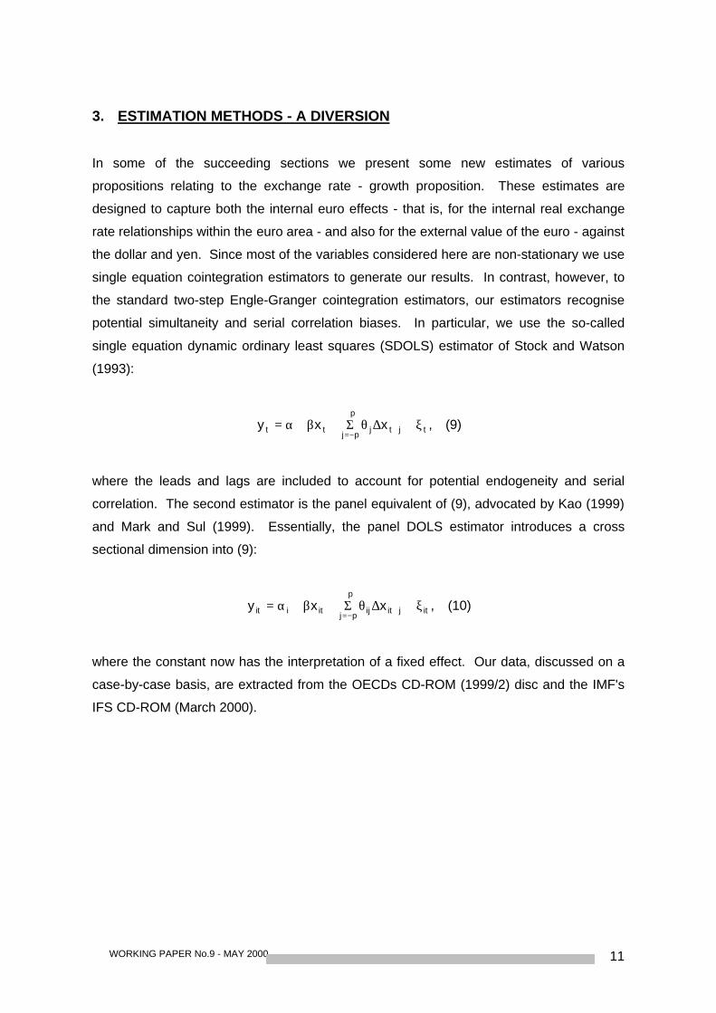
potential simultaneity and serial correlation biases. In particular, we use the so-called
single equation dynamic ordinary least squares (SDOLS) estimator of Stock and Watson
(1993):
,xxy tjtj
p
pjtt ξ+∆θΣ+β+α= +
+
−= (9)
where the leads and lags are included to account for potential endogeneity and serial
correlation. The second estimator is the panel equivalent of (9), advocated by Kao (1999)
and Mark and Sul (1999). Essentially, the panel DOLS estimator introduces a cross
sectional dimension into (9):
,xxy itjitij
p
pjitiit ξ+∆θΣ+β+α= +
+
−= (10)
where the constant now has the interpretation of a fixed effect. Our data, discussed on a
case-by-case basis, are extracted from the OECDs CD-ROM (1999/2) disc and the IMF's
IFS CD-ROM (March 2000).
WORKING PAPER No.9 - MAY 200012
4. EXCHANGE RATE MODELS AND ECONOMIC GROWTH
What is the relationship between income, growth and the exchange rate in macroeconomic
exchange rate models? The flexible price monetary model has become something of a
workhorse in open economy macroeconomics, being the long-run solution to the
celebrated Dornsbusch (1976) overshooting model and a model in its own right (see, for
example, Frenkel (1976) and Mussa (1979)). Although the monetary model is usually
motivated as an asset market model, it is in fact a simple extension of PPP which fleshes
out the determination of prices in each country by imposing continuous money market
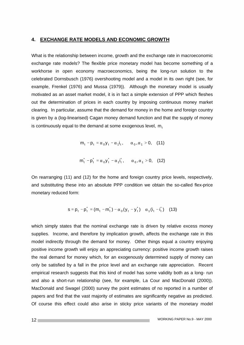
clearing. In particular, assume that the demand for money in the home and foreign country
is given by a (log-linearised) Cagan money demand function and that the supply of money
is continuously equal to the demand at some exogenous level, tm
,0,,iypm 10t1t0tt >ααα−α=− (11)
,0,,iypm 10*t1
*t0
*t
*t >ααα−α=− (12)
On rearranging (11) and (12) for the home and foreign country price levels, respectively,
and substituting these into an absolute PPP condition we obtain the so-called flex-price
monetary reduced form:
)ii()yy()mm(pps *tt1
*tt0
*tt
*tt −α+−α−−=−= (13)
which simply states that the nominal exchange rate is driven by relative excess money
supplies. Income, and therefore by implication growth, affects the exchange rate in this
model indirectly through the demand for money. Other things equal a country enjoying
positive income growth will enjoy an appreciating currency: positive income growth raises
the real demand for money which, for an exogenously determined supply of money can
only be satisfied by a fall in the price level and an exchange rate appreciation. Recent
empirical research suggests that this kind of model has some validity both as a long- run
and also a short-run relationship (see, for example, La Cour and MacDonald (2000)).
MacDonald and Swagel (2000) survey the point estimates of no reported in a number of
papers and find that the vast majority of estimates are significantly negative as predicted.
Of course this effect could also arise in sticky price variants of the monetary model
WORKING PAPER No.9 - MAY 2000 13
(Dornbusch (1976) and Rankel (1979)), and in such models a rise in income can have a
reinforced effect on income to the extent that it pulls up nominal and real interest rates in
the process. The pattern of a strong exchange rate and strong economic growth (weak
exchange rate and weak economic growth) is usually thought of as the business cycle
growth - exchange rate relationship and is usually driven by interest rates. Indeed, to the
extent that interest rates contain information about future growth, the exchange rate can
appreciate in anticipation of strong economic growth.
The above growth - exchange rate relationship may have implications for intra-euro-zone
inflation differentials which are the opposite of those implied by the Balassa-Samuelson
effect, discussed in section 6. For example, with a common euro-zone wide monetary
policy determined in effect by the average income and inflation growth acros the
euro-zone, a country with above (below) average growth will, ceteris paribus, have
negative (positive) inflation. How important is this effect likely to be? The 0α coefficient is
normally estimated at between -0.5 and -1. If we take an average number of -0.75 then
this suggests that a country which has an annualised growth of 1 % above the average of
its euro-zone partners will find its inflation rate falling by 0.75 per cent per annum. Relative
to the inflation numbers mentioned below this effect is rather small but could, nevertheless,
help to offset the implications of increased productivity growth in tradable sectors for
inflation.
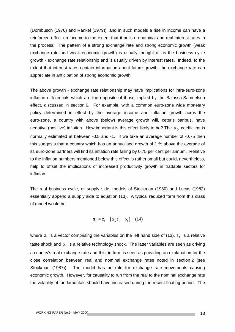
The real business cycle, or supply side, models of Stockman (1980) and Lucas (1982)
essentially append a supply side to equation (13). A typical reduced form from this class
of model would be:
tt0tt t[zs ρ+α+= ], (14)
where tz is a vector comprising the variables on the left hand side of (13), tt is a relative
taste shock and tρ is a relative technology shock. The latter variables are seen as driving
a country's real exchange rate and this, in turn, is seen as providing an explanation for the
close correlation between real and nominal exchange rates noted in section 2 (see
Stockman (1987)). The model has no role for exchange rate movements causing
economic growth. However, for causality to run from the real to the nominal exchange rate
the volatility of fundamentals should have increased during the recent floating period. The
WORKING PAPER No.9 - MAY 200014
fact that they have not is perhaps the most convincing piece of evidence against this class
of model.
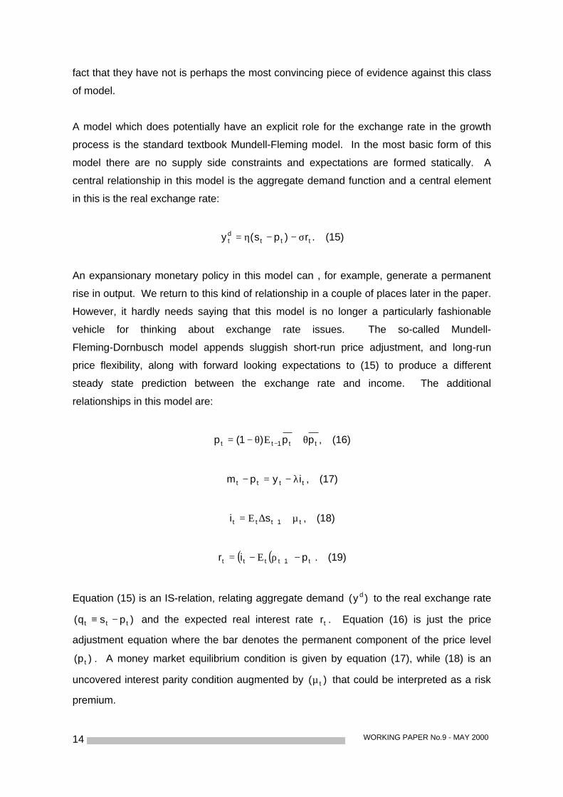
A model which does potentially have an explicit role for the exchange rate in the growth
process is the standard textbook Mundell-Fleming model. In the most basic form of this
model there are no supply side constraints and expectations are formed statically. A
central relationship in this model is the aggregate demand function and a central element
in this is the real exchange rate:
.r)ps(y tttdt σ−−η= (15)
An expansionary monetary policy in this model can , for example, generate a permanent
rise in output. We return to this kind of relationship in a couple of places later in the paper.
However, it hardly needs saying that this model is no longer a particularly fashionable
vehicle for thinking about exchange rate issues. The so-called Mundell-
Fleming-Dornbusch model appends sluggish short-run price adjustment, and long-run
price flexibility, along with forward looking expectations to (15) to produce a different
steady state prediction between the exchange rate and income. The additional
relationships in this model are:
,pp)1(p tt1tt θ+Εθ−= − (16)
,iypm tttt λ−=− (17)
,si t1ttt µ+∆Ε= + (18)
( )( ).pir t1tttt −ρΕ−= + (19)
Equation (15) is an IS-relation, relating aggregate demand )y( d to the real exchange rate
)psq( ttt −≡ and the expected real interest rate tr . Equation (16) is just the price
adjustment equation where the bar denotes the permanent component of the price level
)p( t . A money market equilibrium condition is given by equation (17), while (18) is an
uncovered interest parity condition augmented by )( tµ that could be interpreted as a risk
premium.
WORKING PAPER No.9 - MAY 2000 15
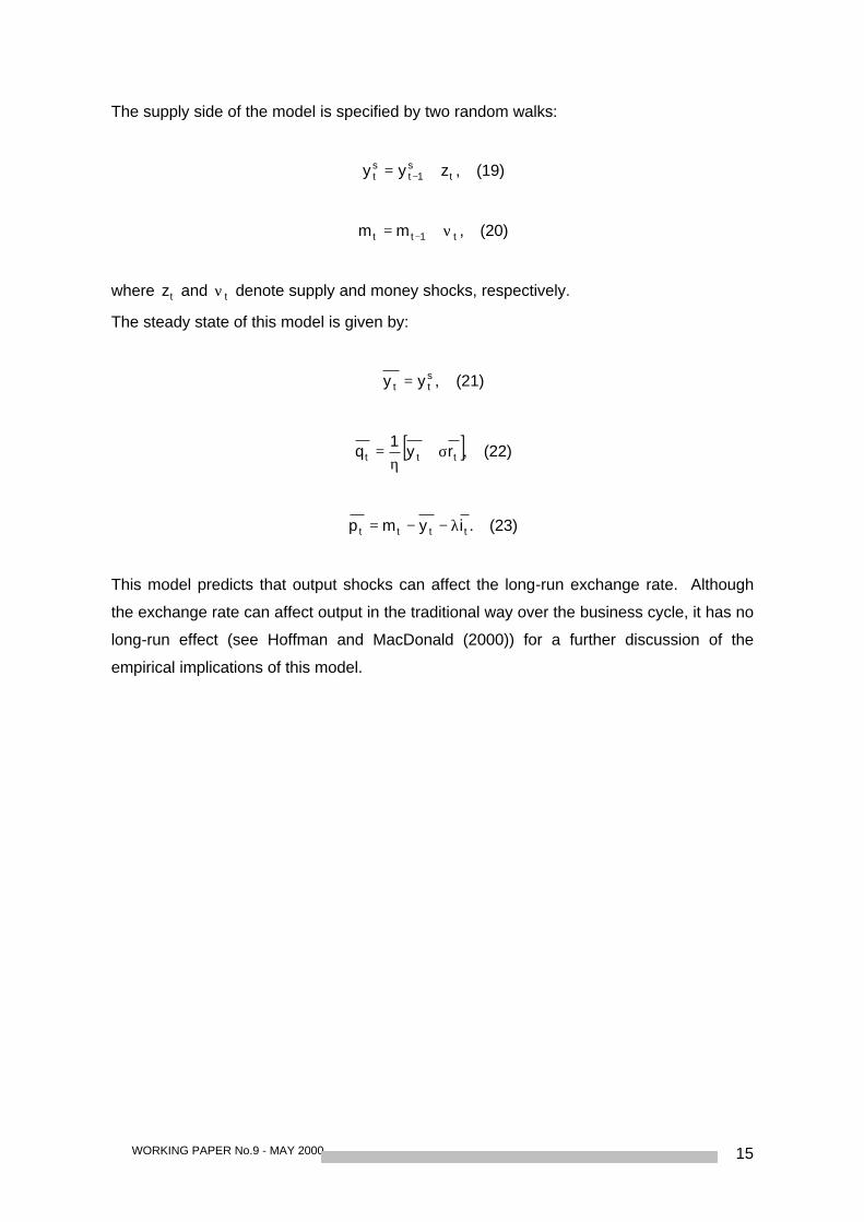
The supply side of the model is specified by two random walks:
,zyy ts
1tst += − (19)
,mm t1tt ν+= − (20)
where tz and tν denote supply and money shocks, respectively.
The steady state of this model is given by:
,yy stt = (21)
[ ],ry1
q ttt σ+η
= (22)
.iymp tttt λ−−= (23)
This model predicts that output shocks can affect the long-run exchange rate. Although
the exchange rate can affect output in the traditional way over the business cycle, it has no
long-run effect (see Hoffman and MacDonald (2000)) for a further discussion of the
empirical implications of this model.
WORKING PAPER No.9 - MAY 200016
5. EXCHANGE RATE REGIMES AND ECONOMIC GROWTH
This brings us into the issue of what has been the exchange rate regime most closely
associated with economic growth. A number of papers have sought to address this issue.
For example, Bordo and Schwartz (1998) provide a comprehensive comparison of the
growth of real per capital income over a number of key regimes of the international
monetary system, spanning the period 1881-1995. The regimes covered are: the classical
gold standard, 1881-1913, the inter-war period 'mixed regime', 1919-1939, the Bretton
Woods period, 1946-1970 and the recent floating rate period, 1973 to present. The
Bretton Woods period is further subdivided into the preconvertible phase, 1946-1958, and
the convertible phase 1959-1970. Also the recent floating period is subdivided into an
inflation period, 1973-1982, and a disinflation period, 1983-1995. In summary, Bordo and
Schwartz find the following: the Bretton Woods period, and particularly the convertible
period, exhibited the most rapid average output growth of any monetary regime and the
inter-war 'mixed regime' period produced the lowest. However, interestingly, taking the
entirety of the Bretton Woods period, their is a higher variability of growth than in the
recent floating rate period.
In contrast, however, Ghosh et al (1996) find that there is little correlation between an
adherence to fixed exchange rates and economic growth, once account is taken of the
1960s period. Indeed, Bordo and Schwartz concede that the link between the kind of fixed
exchange rates provided by Bretton Woods and high economic growth seems less
compelling than for other aspects of economic performance, such as inflation, and they
attribute this to a number of factors. First, they argue that there is an apparent absence of
a link between exchange rate volatility and either investment or trade flows and economic
growth. Thus, although Ghosh et al (1996) find evidence linking real growth to the growth
of investment and trade for pegged countries, they also find total factor productivity growth
to be an important channel of growth for floaters. Furthermore, institutions outwith the
Bretton Woods regime may have been important for growth, such as OEEC, EPU,
European Coal and Steel Community (ECSC). Third, Bordo and Schwartz argue that the
Bretton Woods system may have contributed to growth by providing an overall framework
of rules which allowed Western European nations to solve a hierarchy of co-ordination
problems, which allowed them to encourage investment in growth-generating export
sectors. Fourth, the Bretton Woods regime may have contributed to post-war growth by
being part of an overall package generating political and economic stability - the so-called

WORKING PAPER No.9 - MAY 2000 17
Pax Americana. In their view, therefore, Bordo and Schwartz argue that it is difficult to
disentangle the effects of the exchange rate regime per se from the institutional factors
associated with that regime.
WORKING PAPER No.9 - MAY 200018
6. THE GROWTH - EXCHANGE RATE LINK
We now turn to two potential avenues through which growth can affect the real exchange
rate and, in particular, generate the evident persistence in real exchange rates. The first of
these, the Balassa-Samuelson effect, focuses on the internal price ratio in (6), and argues
that unbalanced growth in a country's traded sector relative to its non-traded sector, can
impart a secular trend into the real exchange rate. This story can have potentially
important implications for the internal relative inflation rates of the euro-zone countries and,
also, for real interest differentials within Europe. Although these relative effects are often
seen in the context of a catch-up hypothesis, and therefore deemed to be only transitory, it
is possible that there may be more permanent implications of these kinds of effects. The
BS hypothesis is also likely to have implications for the external value of the euro. In
particular, what are the implications for the stance of euro-zone monetary policy and,
relatedly, the implications for the kind of exchange rate regime the euro should participate
in? The BS effect is also likely to have important implications for countries, such as the
central european countries, seeking to enter the euro-zone, since sectorally unbalanced
growth can produce exchange rate and inflation combinations which are inconsistent with
the convergence criteria. The Balassa-Samuelson hypothesis is a supply side effect
relating to the longer run trend in the real exchange rate. The second strand in the
growth-exchange rate link considered in this section is more closely associated with the
relative price of traded goods across countries and is related more to the medium run trend
in the real exchange rate. We label this effect the Houthakker-Magee-Krugman
hypothesis, as it was first noted by Houtakker and Magee (1969) and formalised by
Krugman (1989) into the so-called 45° rule. This hypothesis represents a partial
equilibrium approach to interpreting secular trends in real exchange rates. In particular,
the hypothesis suggests that if a particular lock does not hold between a country's relative
growth rate and its relative export and import income elasticities, this could have important
consequences for the secular drift in its exchange rate.
WORKING PAPER No.9 - MAY 2000 19
6.1 Decomposing the real exchange rate: Violations of the LOOP and theBalassa-Samuelson hypothesis
Perhaps the best known explanation for secular trends in the real exchange rate is the
Balassa-Samuelson (BS) biased productivity growth hypothesis. The BS hypothesis
focuses on the role that the so-called internal price ratio - the ratio of non-traded to traded
goods prices - can play in introducing systematic trends into real exchange rates. In
particular, the proposition is that a country with relatively high productivity in its traded
goods sector will have an appreciated real exchange rate, defined using overall price
levels. Furthermore, if that country exhibits relatively high productivity growth in its
tradables sector over time it will have a secular appreciation of its real exchange rate. The
BS hypothesis focuses on the implications of trends in productivity for long-run real
exchange rates, ignoring short-run adjustments. The long-run nature of the model means
that relative prices are driven by supply side factors, with demand side factors being
ignored. The BS hypothesis may be explained in the following way.
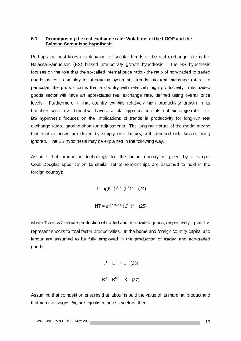
Assume that production technology for the home country is given by a simple
Cobb-Douglas specification (a similar set of relationships are assumed to hold in the
foreign country):
λλ−η= )L()K(T T)1(T (24)
δδ−υ= )L(KNT NT)1(NT (25)
where T and NT denote production of traded and non-traded goods, respectively, η and ν
represent shocks to total factor productivities. In the home and foreign country capital and
labour are assumed to be fully employed in the production of traded and non-traded
goods:
LLL NTT =+ (26)
KKK NTT =+ (27)
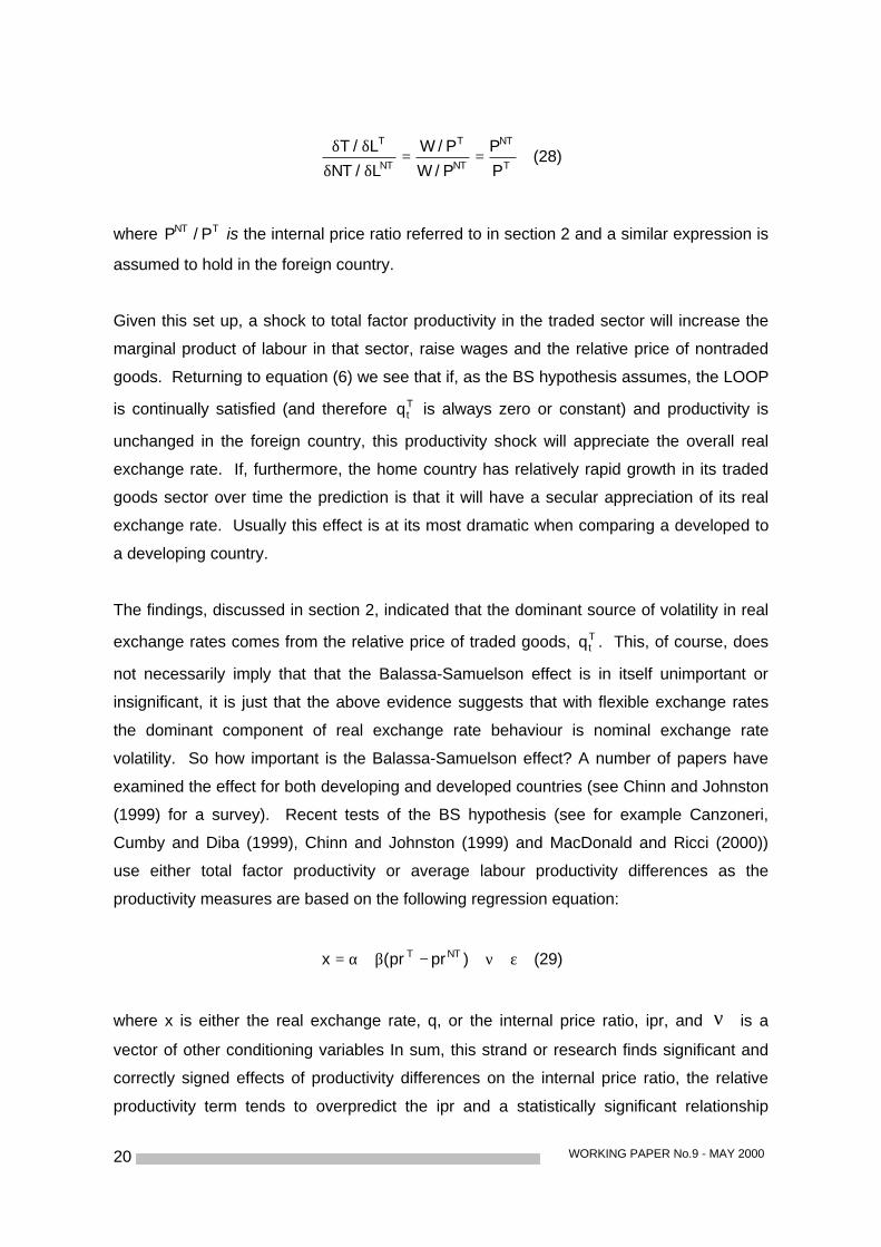
Assuming that competition ensures that labour is paid the value of its marginal product and
that nominal wages, W, are equalised across sectors, then:
WORKING PAPER No.9 - MAY 200020
T
NT
NT
T
NT
T
P
P
P/W
P/W
L/NT
L/T==
δδδδ
(28)
where TNT P/P is the internal price ratio referred to in section 2 and a similar expression is
assumed to hold in the foreign country.
Given this set up, a shock to total factor productivity in the traded sector will increase the
marginal product of labour in that sector, raise wages and the relative price of nontraded
goods. Returning to equation (6) we see that if, as the BS hypothesis assumes, the LOOP
is continually satisfied (and therefore Ttq is always zero or constant) and productivity is
unchanged in the foreign country, this productivity shock will appreciate the overall real
exchange rate. If, furthermore, the home country has relatively rapid growth in its traded
goods sector over time the prediction is that it will have a secular appreciation of its real
exchange rate. Usually this effect is at its most dramatic when comparing a developed to
a developing country.
The findings, discussed in section 2, indicated that the dominant source of volatility in real
exchange rates comes from the relative price of traded goods, Ttq . This, of course, does
not necessarily imply that that the Balassa-Samuelson effect is in itself unimportant or
insignificant, it is just that the above evidence suggests that with flexible exchange rates
the dominant component of real exchange rate behaviour is nominal exchange rate
volatility. So how important is the Balassa-Samuelson effect? A number of papers have
examined the effect for both developing and developed countries (see Chinn and Johnston
(1999) for a survey). Recent tests of the BS hypothesis (see for example Canzoneri,
Cumby and Diba (1999), Chinn and Johnston (1999) and MacDonald and Ricci (2000))
use either total factor productivity or average labour productivity differences as the
productivity measures are based on the following regression equation:
ε+ν+−β+α= )prpr(x NTT (29)
where x is either the real exchange rate, q, or the internal price ratio, ipr, and ν is a
vector of other conditioning variables In sum, this strand or research finds significant and
correctly signed effects of productivity differences on the internal price ratio, the relative
productivity term tends to overpredict the ipr and a statistically significant relationship
WORKING PAPER No.9 - MAY 2000 21
between relative productivity differences and the overall real exchange rate is found,
especially if a panel estimator is used (and the relative productivity term tends to
underpredict the real exchange rate) .
Canzoneri, Diba and Eudey (1996) test the BS hypothesis for a group of eleven European
countries (Austria, Belgium, Denmark, Finland, France, Germany, Italy, Portugal, Spain
and Sweden) using annual data on average labour productivity in the traded and
non-traded sectors for the period 1970 to 1990. Using some simple statistical tests and
single equation cointegration tests Canzoneri et al show compelling evidence to suggest
that trends in the productivity ratio are good predictors of long-run trends in overall real
exchange rates. Kohler (1999) uses an unbalanced panel data set of 28 countries for the
period 1960-1997 to examine how important sectoral productivity is in explaining past price
movements. Using a standard fixed effects panel estimator she finds slope coefficients
which are significantly above zero but also significantly below unity (a range of
approximately 0.5 and 0.7) and interprets this as a reflection of a failure of wage
equalisation across countries (some support for this is to be found in Aleberola and
Tyrvainen (1998) who show that conditioning on this differential produces a coefficient on
the relative productivity term of unity). Additionally, using the panel cointegration estimator
of Pedroni, which allows for the estimation of the individual BS coefficients for each
country, Kohler finds a fairly wide dispersion of point estimates ranging from -I for Italy,
Belgium and Finland to -0.6 for Germany.
We interpret the above evidence as suggesting that the Balassa-Samuelson hypothesis is
in the data for euro-zone countries. What, if any, are the likely consequences for this for
the future of EMU? In particular, what are the implications for the behaviour of real
exchange rates and inflation within the euro-zone and also for the euro-zone relative to its
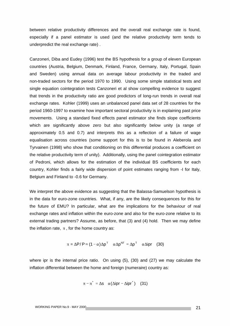
external trading partners? Assume, as before, that (3) and (4) hold. Then we may define
the inflation rate, π , for the home country as:
iprppp)1(P/P TNTT ∆α+∆=∆α+∆α−≈∆≡π (30)
where ipr is the internal price ratio. On using (5), (30) and (27) we may calculate the
inflation differential between the home and foreign (numeraire) country as:
)ipripr(s ** ∆−∆α+∆=π−π (31)
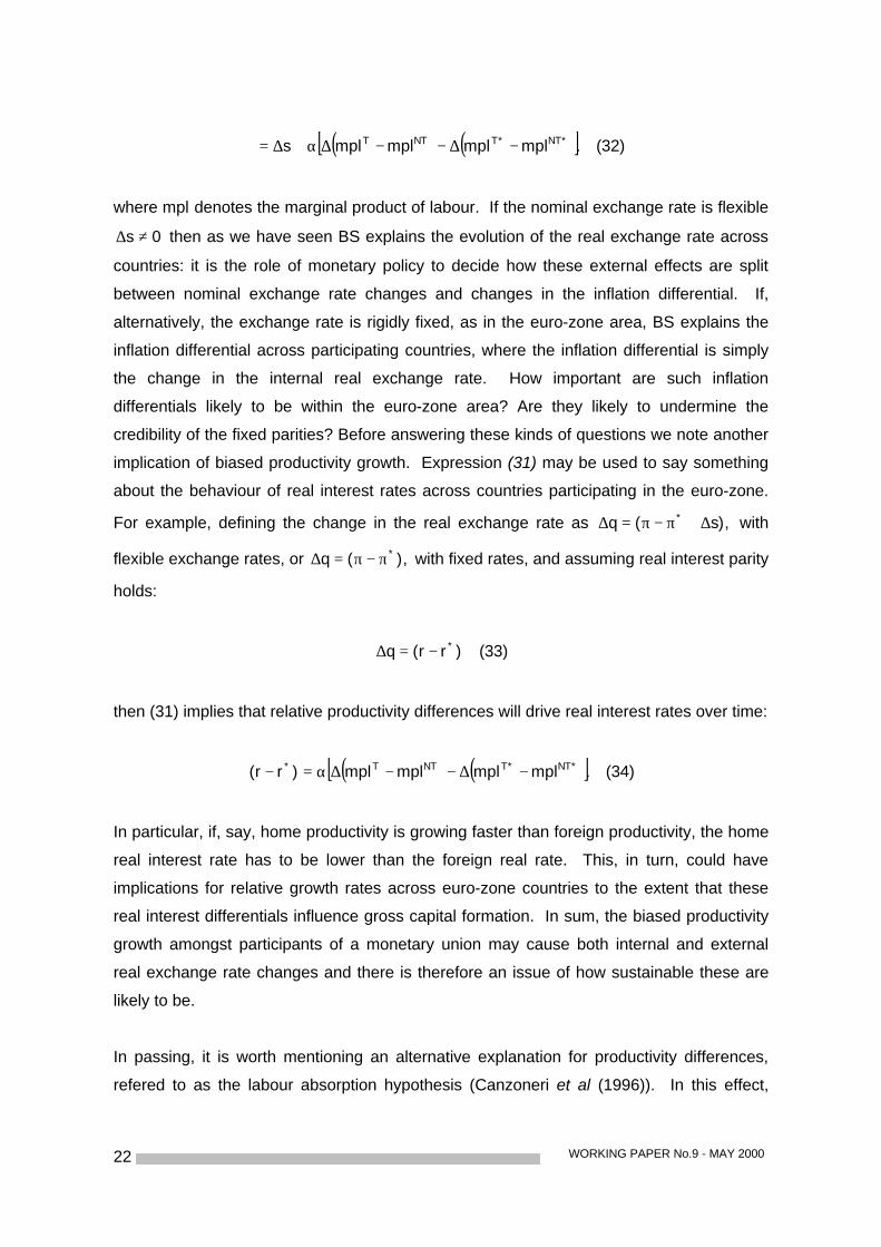
WORKING PAPER No.9 - MAY 200022
( ) ( )[ ].mplmplmplmpls *NT*TNTT −∆−−∆α+∆= (32)
where mpl denotes the marginal product of labour. If the nominal exchange rate is flexible
0s ≠∆ then as we have seen BS explains the evolution of the real exchange rate across
countries: it is the role of monetary policy to decide how these external effects are split
between nominal exchange rate changes and changes in the inflation differential. If,
alternatively, the exchange rate is rigidly fixed, as in the euro-zone area, BS explains the
inflation differential across participating countries, where the inflation differential is simply
the change in the internal real exchange rate. How important are such inflation
differentials likely to be within the euro-zone area? Are they likely to undermine the
credibility of the fixed parities? Before answering these kinds of questions we note another
implication of biased productivity growth. Expression (31) may be used to say something
about the behaviour of real interest rates across countries participating in the euro-zone.
For example, defining the change in the real exchange rate as ),s(q * ∆+π−π=∆ with
flexible exchange rates, or ),(q *π−π=∆ with fixed rates, and assuming real interest parity
holds:
)rr(q *−=∆ (33)
then (31) implies that relative productivity differences will drive real interest rates over time:
( ) ( )[ ].mplmplmplmpl)rr( *NT*TNTT* −∆−−∆α=− (34)
In particular, if, say, home productivity is growing faster than foreign productivity, the home
real interest rate has to be lower than the foreign real rate. This, in turn, could have
implications for relative growth rates across euro-zone countries to the extent that these
real interest differentials influence gross capital formation. In sum, the biased productivity
growth amongst participants of a monetary union may cause both internal and external
real exchange rate changes and there is therefore an issue of how sustainable these are
likely to be.
In passing, it is worth mentioning an alternative explanation for productivity differences,
refered to as the labour absorption hypothesis (Canzoneri et al (1996)). In this effect,
WORKING PAPER No.9 - MAY 2000 23
increased integration in Europe has forced the traded goods sector to become more
competitive and should shed excess labour. This surplus labour has been absorbed by
government employment, thereby reducing average productivity of the nontraded sector
and, since this sector is sheltered from competition, increasing the price. However,
Canzoneri et al argue that for this effect to be a valid explanation of real exchange rate
movements within Europe would require the real exchange rates to overpredict productivity
trends (which are proxies for marginal costs); however, in their work the opposite appears
to be the case.
How important is the BS effect likely to be for the euro-zone? A number of studies have
examined the kind of relative price movements which seem to be consistent with the
operation of existing monetary unions. For example, De Grauwe (1992) examines the
relative price behaviour of five German Lander and finds inflation differentials between 0.2
and 1.2 per cent. Poloz (1990), Bayoumi and Thomas (1995) and Buti and Sapir (1998)
examine inflation differentials within Canada and the United States, respectively, and find
inflation differentials of between 0.5 and 2 per cent. Canzoneri et al (1996) use their
estimated productivity equations discussed above to calculate the inflation differentials of
their group of European countries relative to Germany implied by the trends in relative
labour productivity. The countries can be divided into three groups: Belgium, Italy and
Spain form a group in which productivity trends imply that they should have inflation rates
which are about 2 % higher than German rates, while the relative productivity growths of
Portugal, Denmark, Austria, France, UK and Sweden imply they should have inflation rates
on average 1 % higher than German rates and Finland should have an inflation rate about
the same as the German average. These kind of inflation differentials are not inconsistent
with the Maastricht criterion, nor do they seem to be inconsistent with the size of
differentials found within existing monetary unions, referred to above. Based on her
estimates of productivity differentials, discussed above, Kholer (1999) estimates implied
inflation (CP1) differentials for EMU countries. She finds that the upper band for this is in
the range 1-3% with the higher figure representing the growth experience over the last 30
years, and the smaller number being derived from the growth experience over the last 15
years.
Although the inflation differentials implied by relative productivity growth rates do not seem
inconsistent with inflation differentials in existing monetary unions, Canzoneri et al use the
data set of Bayoumi and Eichengreen (1993) to demonstrate that there is much less
regional variation in productivity within the US and indeed that the implied differentials in
WORKING PAPER No.9 - MAY 200024
regional inflation are only about one fifth the size of Europe. Do countries with differing
productivity trends belong in the same monetary union? Will full economic integration
cause productivity trends to converge in Europe? We would argue that indeed this is what
has caused the homogeneity in existing monetary unions.
We present some new empirical evidence on the importance of the Balassa-Samuelson
hypothesis for the euro~zone area by running the following regression using a single
equation DOLS estimator:
.qq tT,NT
tt ε+β+α= (35)
In order for this equation to represent a test of the BS hypothesis we must assume that the
LOOP holds up to a constant and that the internal price ratio is picking up productivity
differences and not other demand side factors. However, even if it is not a pure test of BS
it may nevertheless be instructive in indicating the importance of the internal price ratio in
driving internal and external real exchange rates for the euro-zone. If the BS is valid, the
β coefficient is expected to be significantly negative. As is standard in the exchange rate
literature, we proxy the price of traded goods with the producer price index and the
consumer price index is our proxy for non-traded goods. These data were extracted from
the International Monetary Fund's International Financial Statistics CD-ROM (March 2000).
We present sets of estimates for three sample periods. The full sample period,
1980q1-1998q4, and two sub-periods, 1980q1-1989q4, and 1990q1-1998q4. Estimating
this relationship for the two sub-samples should give some indication of the stability of the
relationship and, in particular, if the convergence process has affected it. The countries
chosen for these tests are listed in Table 4 and most are members of the euro-zone area.
Three numeraire currencies have been chosen for these tests: the US dollar, the Japanese
yen and the German mark. The former two rates pick up the external euro real exchange
rate, while the latter picks up the behaviour of internal real exchange rates.
For the US dollar and yen based systems we note that for the full sample period, and the
two sub-samples, the majority of coefficients are correctly signed and statistically
significant. We note also that in the majority of cases the coefficient for these two external
systems suggests that a one per cent increase in the internal price ratio has a more than
proportionate effect on the real exchange rate and this effect seems to be stable across
the sub-samples. For the system based on the mark, we note that the majority of
coefficients are correctly signed and significant but that for the full sample the absolute
WORKING PAPER No.9 - MAY 2000 25
magnitude of the coefficients is less than unity indicating that a one percent rise in T,NTtq
has a less than proportionate effect on the overall real exchange rate. The results for the
first sub-sample are similar to the full sample but in the second sample we note a number
of coefficients are above unity and these tend to be for countries most likely to be involved
in a catch-up process -Spain Italy and Ireland.
Panel DOLS estimates are constructed solely for the participants of the euro-zone area
(that is excluding both Denmark and the UK) and are reported in Table 5. These results
generally confirm the points made regarding the single equation estimates.
In sum, the results based on equation (35) suggest that the there is a significant and
correctly signed Balassa-Samuelson effect for the internal real exchange rates of
euro-zone countries and that the magnitude of this effect does not appear to be
inconsistent with these countries participation in a monetary union. Furthermore, there
also seems to be a correctly signed and significant Balassa-Samuleson effect for
euro-zone countries relative to the two key external currencies. The larger magnitude of
the external effect would perhaps suggest that the external nominal value of the euro
should be flexible.
We conclude this section by arguing that the existence of productivity differentials within
Europe is unlikely to generate movements of internal real exchange rates which would put
a strain on EMU. There will, however, inevitably be important and, perhaps significant,
differences in the short-run as countries catch-up with their monetary union partners (and
Ireland is a classic example of this at the moment), but once such countries have caught
up the differentials would not be expected to be any larger than those observed for existing
monetary unions. If agents do indeed recognise that these inflation differentials are
transitory it would seem unlikely that the implied real interest differentials will have
significant implications for differential capital formation. To they extent that they do, this
could actually moderate the internal real exchange rate movements to the extent that they
increase productivity in the service sectors. At the end of the day the importance of the
Balassa-Samuelson effect in the euro-zone context boils down to whether it is seen as a
good or a bad in the European context. It would seem that one of the key rationales for
EMU is to allow countries which were originally relatively poor to catch up. Fundamentally,
what EMU does is to allow countries to trade-off real exchange rate variation due to
nominal variability from Tq for variability due to .q T,NT As we shall argue subsequently,
WORKING PAPER No.9 - MAY 200026
the former is unambiguously bad, whereas the latter is a natural consequence of the
catch-up process and is likely to be a transitory phenomenon.
6.2 The Houthakker-Magee-Krugman 45° Rule
Perhaps the relationship that many economists would reach for first when trying to think
about the implications of growth differences across countries for real exchange rates is the
standard partial equilibrium analysis of trade flows. Ceteris paribus, a relatively fast
growing country should have a depreciating exchange rate for the maintenance of current
account balance, while a relatively slow growing country should have an appreciating
exchange rate. However, Houthaker and Magee (1969) first noted that this need not be
the case if the slow growing country has a sufficiently favourable income elasticity of
demand for its exports relative to its income elasticity of demand for imports. Krugman
(1989) formalised this relationship into the so-called 45° rule: unless the relative growth
rate between the home country and the rest of the world is equal to the ratio of relative
income elasticities of demand, the country's real exchange rate will exhibit a long-run
trend. We label this hypothesis the Houthakker-Magee-Krugman (HMK) relationship. In
contrast to the Balassa-Samuelson hypothesis, which focuses exclusively on supply side
effects in trying to understand secular movements of real exchange rates, the HMK
approach focusses exclusively on demand side effects. It is also distinct from the
Balsassa-Samuelson hypothesis in shifting the emphasis for secular movements in the
real exchange rate from the internal price ratio to the external price ratio: traded goods are
no longer perfect substitutes across countries and so systematic movements in their
relative price can explain systematic elements in the real exchange rate.
To illustrate the HMK hypothesis, we use a standard partial equilibrium analysis of trade
flows. Define the real exchange rate in natural units (instead of logarithms) as: q = sp*/p,
where p now relates to the price of output. A standard trade balance model may be written
as follows, where export volume is assumed to depend of foreign output and the relative
price of domestic goods:
*),y,q(xx = (36)
and import volume is assumed to depend on domestic income and the relative price term:
WORKING PAPER No.9 - MAY 2000 27
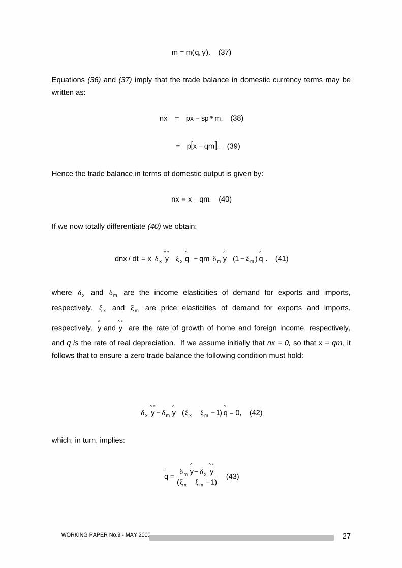
).y,q(mm = (37)
Equations (36) and (37) imply that the trade balance in domestic currency terms may be
written as:
,msppxnx ∗−= (38)
[ ].qmxp −= . (39)
Hence the trade balance in terms of domestic output is given by:
.qmxnx −= (40)
If we now totally differentiate (40) we obtain:
.q)1(yqmqyxdt/dnx^
m
^
m
^
x
^*
x
ξ−+δ−
ξ+δ= (41)
where xδ and mδ are the income elasticities of demand for exports and imports,
respectively, xξ and mξ are price elasticities of demand for exports and imports,
respectively, ^*^yandy are the rate of growth of home and foreign income, respectively,
and q is the rate of real depreciation. If we assume initially that nx = 0, so that x = qm, it
follows that to ensure a zero trade balance the following condition must hold:
,0q)1(yy^
mx
^
m
^*
x =−ξ+ξ+δ−δ (42)
which, in turn, implies:
)1(yy
qmx
^*
x
^
m^
−ξ+ξδ−δ
= (43)
WORKING PAPER No.9 - MAY 200028
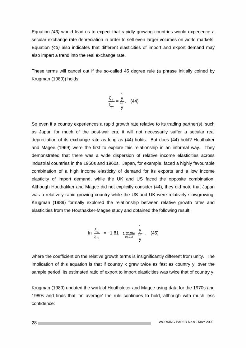
Equation (43) would lead us to expect that rapidly growing countries would experience a
secular exchange rate depreciation in order to sell even larger volumes on world markets.
Equation (43) also indicates that different elasticities of import and export demand may
also impart a trend into the real exchange rate.
These terms will cancel out if the so-called 45 degree rule (a phrase initially coined by
Krugman (1989)) holds:
.y
y^*
^
m
x =ξξ
(44)
So even if a country experiences a rapid growth rate relative to its trading partner(s), such
as Japan for much of the post-war era, it will not necessarily suffer a secular real
depreciation of its exchange rate as long as (44) holds. But does (44) hold? Houthaker
and Magee (1969) were the first to explore this relationship in an informal way. They
demonstrated that there was a wide dispersion of relative income elasticities across
industrial countries in the 1950s and 1960s. Japan, for example, faced a highly favourable
combination of a high income elasticity of demand for its exports and a low income
elasticity of import demand, while the UK and US faced the opposite combination.
Although Houthakker and Magee did not explicitly consider (44), they did note that Japan
was a relatively rapid growing country while the US and UK were relatively slowgrowing.
Krugman (1989) formally explored the relationship between relative growth rates and
elasticities from the Houthakker-Magee study and obtained the following result:
,y
y81.1ln
^*
^
)21.0(m
x ln210.1
+−=
ξξ
(45)
where the coefficient on the relative growth terms is insignificantly different from unity. The
implication of this equation is that if country x grew twice as fast as country y, over the
sample period, its estimated ratio of export to import elasticities was twice that of country y.
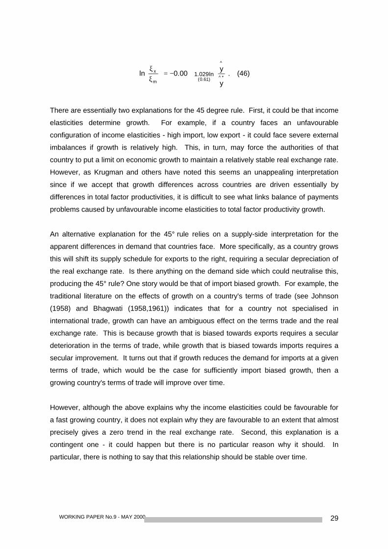
Krugman (1989) updated the work of Houthakker and Magee using data for the 1970s and
1980s and finds that 'on average' the rule continues to hold, although with much less
confidence:
WORKING PAPER No.9 - MAY 2000 29
.y
y00.0ln
^*
^
)61.0(m
x ln029.1
+−=
ξξ
(46)
There are essentially two explanations for the 45 degree rule. First, it could be that income
elasticities determine growth. For example, if a country faces an unfavourable
configuration of income elasticities - high import, low export - it could face severe external
imbalances if growth is relatively high. This, in turn, may force the authorities of that
country to put a limit on economic growth to maintain a relatively stable real exchange rate.
However, as Krugman and others have noted this seems an unappealing interpretation
since if we accept that growth differences across countries are driven essentially by
differences in total factor productivities, it is difficult to see what links balance of payments
problems caused by unfavourable income elasticities to total factor productivity growth.
An alternative explanation for the 45° rule relies on a supply-side interpretation for the
apparent differences in demand that countries face. More specifically, as a country grows
this will shift its supply schedule for exports to the right, requiring a secular depreciation of
the real exchange rate. Is there anything on the demand side which could neutralise this,
producing the 45° rule? One story would be that of import biased growth. For example, the
traditional literature on the effects of growth on a country's terms of trade (see Johnson
(1958) and Bhagwati (1958,1961)) indicates that for a country not specialised in
international trade, growth can have an ambiguous effect on the terms trade and the real
exchange rate. This is because growth that is biased towards exports requires a secular
deterioration in the terms of trade, while growth that is biased towards imports requires a
secular improvement. It turns out that if growth reduces the demand for imports at a given
terms of trade, which would be the case for sufficiently import biased growth, then a
growing country's terms of trade will improve over time.
However, although the above explains why the income elasticities could be favourable for
a fast growing country, it does not explain why they are favourable to an extent that almost
precisely gives a zero trend in the real exchange rate. Second, this explanation is a
contingent one - it could happen but there is no particular reason why it should. In
particular, there is nothing to say that this relationship should be stable over time.
WORKING PAPER No.9 - MAY 200030
The new trade theory of Krugman (1980) and others offers an alternative supply-side
explanation for the 450 rule. In particular, Krugman argues that the specialisation among
industrial countries is primarily due to increasing returns (i.e. the inherent advantages of
specialisation itself) rather than the traditional concept of comparative advantage.
Relatively fast growing economies expand their share of world markets by expanding the
range of goods their country produces rather than reducing the relative price of their
goods. In this view 'imports' and 'exports are seen as aggregates whose composition
changes over time as more goods are added to the list. So, for example, the euro-zone's
exports face a downward sloping demand curve at any point in time, but as the euro-zone
economy grows over time the definition of the aggregate changes in such a way as to
make the apparent demand curve shift outwards (as the supply shifts down) and therefore
there is no need for a secular depreciation of the real exchange rate4.
To what extent is the 45° relationship in the data for our euro-zone countries? In order to
make our estimates comparable with those of Houthakker, Magee and Krugman we have
used compatable specifications of export and import functions. In particular, the volume of
imports is assumed to be a function of home CDP, in constant prices, and the relative price
of manufactures imports, calculated as the ratio of manufacturers import unit value to the
GDP deflator. The volume of exports is assumed to be a function of 'foreign' real CDP and
the OECD index of the relative export price of manufactures. We used four alternative
measures of foreign GDP: the eu15 geometric average of real GDP, German real G13P,
OECD total real GDP and US real GDR The first two measures are designed to capture
the CDP of the internal euro-zone trading partners, whereas the latter two are intended to
capture the CDP of the external trading partners - the idea being that there may be a
different internal and external effects for the currencies. The sample period is 1980,
quarter 1 through to 1998 quarter 4 and all data have been extracted from the OECD
database. It turns out that for the external income measures, there was practically no
difference between the point estimates obtained using the OECD and US GDPs, and
therefore we only report the numbers for the US, The estimated import and export
functions are not reported here, but all of them had correctly signed and significant income
elasticities and most had correctly signed relative price effects, although the significance
levels of these were rather mixed.
4 Krugman (1988) uses a Dicit-Stiglitz model in which two economies trade with each other but grow at different rates. In
such a model the relative prices of the representative goods produced in each country will remain unchanged and so anydifferences in export and import growth are attributable to income elasticity differences.
WORKING PAPER No.9 - MAY 2000 31
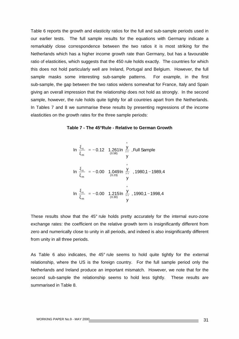
Table 6 reports the growth and elasticity ratios for the full and sub-sample periods used in
our earlier tests. The full sample results for the equations with Germany indicate a
remarkably close correspondence between the two ratios it is most striking for the
Netherlands which has a higher income growth rate than Germany, but has a favourable
ratio of elasticities, which suggests that the 450 rule holds exactly. The countries for which
this does not hold particularly well are Ireland, Portugal and Belgium. However, the full
sample masks some interesting sub-sample patterns. For example, in the first
sub-sample, the gap between the two ratios widens somewhat for France, Italy and Spain
giving an overall impression that the relationship does not hold as strongly. In the second
sample, however, the rule holds quite tightly for all countries apart from the Netherlands.
In Tables 7 and 8 we summarise these results by presenting regressions of the income
elasticities on the growth rates for the three sample periods:
Table 7 - The 45°Rule - Relative to German Growth
=
ξξ
m
xln SampleFull,y
yln261.112.0
^*
^
)58.0(
+−
=
ξξ
m
xln 4,19891,1980,y
yln049.100.0
^*
^
)23.0(−
+−
=
ξξ
m
xln 4,19981,1990,y
yln215.100.0
^*
^
)30.0(−
+−
These results show that the 45° rule holds pretty accurately for the internal euro-zone
exchange rates: the coefficient on the relative growth term is insignificantly different from
zero and numerically close to unity in all periods, and indeed is also insignificantly different
from unity in all three periods.
As Table 6 also indicates, the 45° rule seems to hold quite tightly for the external
relationship, where the US is the foreign country. For the full sample period only the
Netherlands and Ireland produce an important mismatch. However, we note that for the
second sub-sample the relationship seems to hold less tightly. These results are
summarised in Table 8.
WORKING PAPER No.9 - MAY 200032
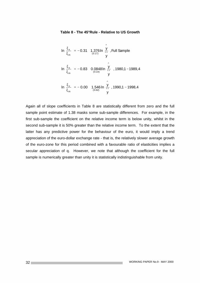
Table 8 - The 45°Rule - Relative to US Growth
=
ξξ
m
xln SampleFull,y
yln376.131.0
^*
^
)17.0(
+−
=
ξξ
m
xln 4,19891,1980,y
yln0848.083.0
^*
^
)14.0(−
+−
=
ξξ
m
xln 4,19981,1990,y
yln546.100.0 ^*
^
)62.0(−
+−
Again all of slope coefficients in Table 8 are statistically different from zero and the full
sample point estimate of 1.38 masks some sub-sample differences. For example, in the
first sub-sample the coefficient on the relative income term is below unity, whilst in the
second sub-sample it is 50% greater than the relative income term. To the extent that the
latter has any predictive power for the behaviour of the euro, it would imply a trend
appreciation of the euro-dollar exchange rate - that is, the relatively slower average growth
of the euro-zone for this period combined with a favourable ratio of elasticities implies a
secular appreciation of q. However, we note that although the coefficient for the full
sample is numerically greater than unity it is statistically indistinguishable from unity.
WORKING PAPER No.9 - MAY 2000 33
7. THE EXCHANGE RATE - GROWTH LINK
In this section we examine the causality link running from the exchange rate to growth.
There are two main components here: the effect of exchange rates on economic growth,
through their influence on international trade, and the effects of exchange rate movements
on investment. As we shall see there are a number of important overlaps between these
topics.
7.1 Exchange rates and international trade
7.1.1 Theory
In the introduction we noted that the effects of exchange rate movements on international
trade may be one way in which the exchange rate can affect economic growth. The
beneficial effects of international trade on a country's welfare have been discussed
extensively in the economics literature at least since Adam Smith's famous example of
specialisation due to comparative advantage. Such specialisation can affect growth by
changing the allocation of resources across industrial sectors; i.e. if sectors have different
equilibrium growth rates then specialisation due to comparative advantage could affect the
economy's overall growth rate. The trade literature also suggests a number of additional
channels, which have their effect at the sectoral level, such as: the ability of a country to
exploit increasing returns due to the exposure to larger markets; the transferance of
technology across countries, through exposure to new goods and also investment; trade
may cause a spillover of ideas across countries, thereby raising the productivity of
research; and by increasing the size of the market may increase the incentive of
researchers to undertake research5. Furthermore, the role of export-led growth and import
substitution are sometimes discussed in policy circles as important driving forces for
economic growth. But how does the exchange rate affect international trade and therefore
growth?
5 Proudman and Redding (1996) asess the consequences of these different effects for growth in the UK in the 1970s and
conclude that comparative advantage itself is unlikely to explain the relatively fast growth of manufacturing output in the1970s. This study is discussed in more detail below.
WORKING PAPER No.9 - MAY 200034
The main way in which exchange rate movements affect trade is through their impact on
the profitability of companies engaged in international trade, or those considering engaging
in international trade. Here we distinguish a level and a volatility effect. The levels effect,
which is essentially the effect contained in traditional open economy macroeconomic
models, suggests that there is a positive relationship between the level of the real
exchange rate and growth. For example, starting from a position where PPP, or some
other measure of the equilibrium exchange rate, holds, a depreciation of the nominal
exchange rate will likely produce a change in the real exchange rate which is persistent.
The depreciation of the nominal and real exchange rates could, in turn, imply strong
relative price changes for exports and import competing goods. For example, an
exchange rate depreciation, by increasing the profitability of domestic producers, could
lead them to work the existing capital stock more intensively in the short term and, to the
extent that such effects persist, increase investment in the medium term. An appreciation
of the domestic currency could have the opposite effects, initially reducing the utilisation of
the existing capital stock, reducing investment and eventually perhaps leading to the
closure of the existing capital stock. Perhaps the best known example of the latter is the
consequences of the tight monetary policy pursued in the late 1970s/ early 1980s by the
Thatcher government in the UK. It is now widely accepted that the real an nominal
exchange rate overshoots as a consequence of this policy led to around twenty per cent of
the UKs traded sector being shut down.
However, the above discussion of the effects of the level of an exchange rate on a
country's trade and growth ignores a number of broader factors. First, it ignores the
implications of exchange rate changes for the cost of imported intermediate inputs into
production. The inclusion of the latter into the calculation of the effects of exchange rate
changes can produce offsets to the effects on price and quantity. Of course these kinds of
effects are specific to the firm or, more generally, to the tradable sector. There will be
wider macroeconomic consequences of the initial exchange rate movement which could
offset or perhaps even reverse the initial effects. For example, the reduction of real
income associated with a depreciation may at least, in part, offset the expansionary effects
coming from the traded sector. So the results of what we are calling the level effect on
trade and growth may well be ambiguous for a particular country. Furthermore, the net
effects on international trade of the levels effect are also likely to be ambiguous since a
depreciation in one country will have a counter part in a foreign country. Perhaps it is
because of the ambiguous nature of the levels effect that has led most commentators to
WORKING PAPER No.9 - MAY 2000 35
focus on the effect of exchange rate volatility on international trade and growth. At first
blush the effects of volatility on international trade seems unambiguous.
The early literature on the relationship between exchange rate volatility and trade
suggested a negative relationship; that is, the volatility that is so evident when exchange
rates are flexible has a deleterious effect on international trade. This negative association
is usually refered to as the traditional relationship. For example, the early theoretical
literature on the implications of volatility for trade focussed on the combination of a risk
averse trading company and the uncertainty of exchange rate movements reducing both
trade and output (see, for example, Ethier (1973), Artus (1983) and Brodsky (1984)). The
basic idea in these papers may be summarised in the following way. Exchange rate risk is
assumed to be the main source of profit risk for a risk averse firm. So as exchange rate
volatility increases, profit risk will also increase and for a risk averse firm this reduces the
benefits of international trade and therefore ultimately the volume of international trade.
Demers (1991) showed how even in the presence of risk neutral agents a negative
association between volatility and trade can be generated. For example, a risk neutral firm
which is uncertain about the state of demand due to exchange rate driven price uncertainty
will cut back its production and trade volumes if it has undertaken an irreversible
investment in physical capital.
However, a number of papers have demonstrated that the effect of exchange rate volatility
on trade is not as clear-cut as the above discussion might suggest. For example, De
Grauwe (1988) considers a variant of the Newbery-Stiglitz model of production and
consumption with a risk averse exporter. He shows that although an increase in risk
unambiguously decreases welfare in this kind of model it can also lead the exporter to
increase exports depending on how risk averse he or she is. Essentially this result comes
about because of the interaction between an income and substitution effect. The former is
the effect which usually comes to mind when one thinks about the effects of risk on trade -
an increase in risk lowers the attractiveness of these activities and leads firms to reduce
them. The income effect leads to the opposite outcome - when risk increases the
expected total utility of export revenues declines. However, this fall can be offest by
increasing resources in the export sector and, if the income effect dominates the
substitution effect, higher exchange risk can generate increased export activity.
An alternative way of generating a positive association between exchange rate volatility
and trade is to appeal to the 'new' theory of investment. For example, Franke (1991),
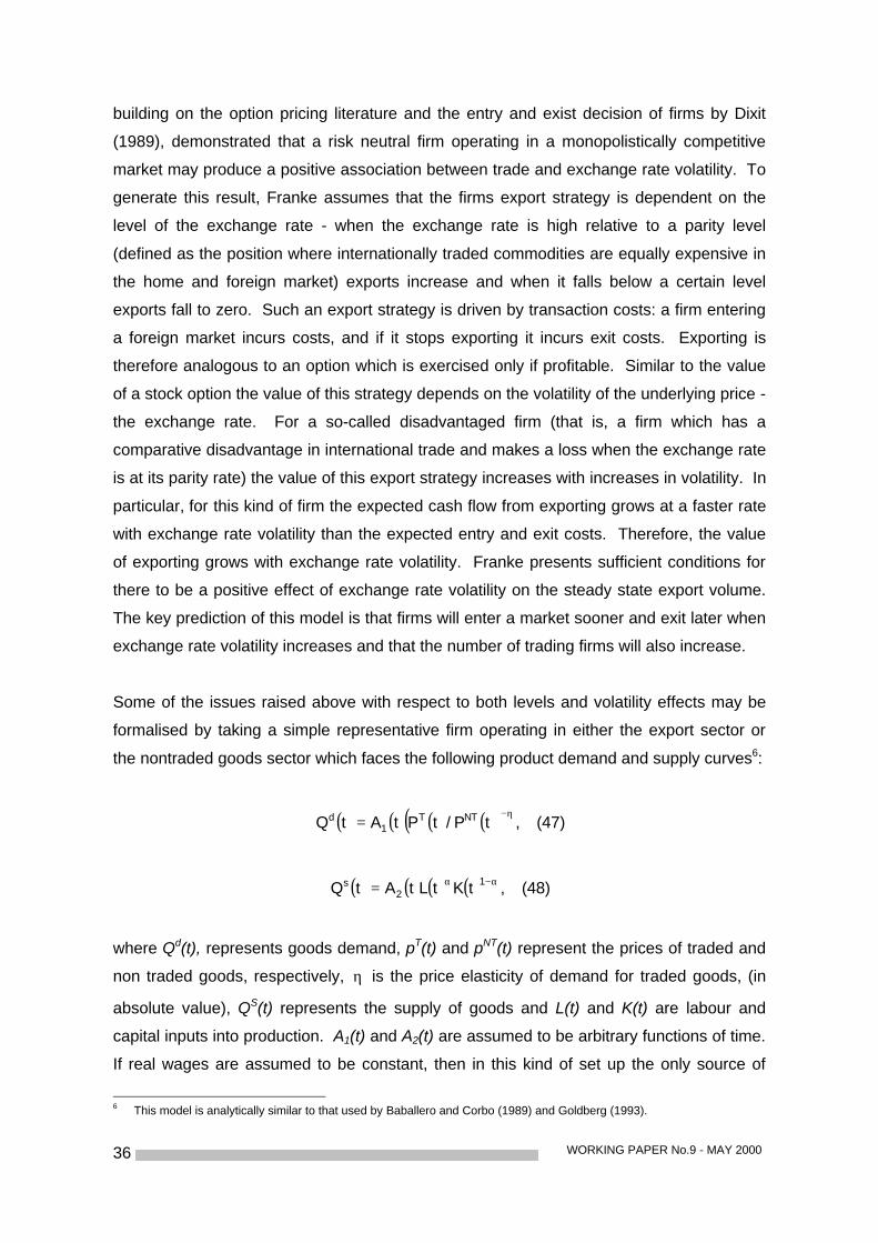
WORKING PAPER No.9 - MAY 200036
building on the option pricing literature and the entry and exist decision of firms by Dixit
(1989), demonstrated that a risk neutral firm operating in a monopolistically competitive
market may produce a positive association between trade and exchange rate volatility. To
generate this result, Franke assumes that the firms export strategy is dependent on the
level of the exchange rate - when the exchange rate is high relative to a parity level
(defined as the position where internationally traded commodities are equally expensive in
the home and foreign market) exports increase and when it falls below a certain level
exports fall to zero. Such an export strategy is driven by transaction costs: a firm entering
a foreign market incurs costs, and if it stops exporting it incurs exit costs. Exporting is
therefore analogous to an option which is exercised only if profitable. Similar to the value
of a stock option the value of this strategy depends on the volatility of the underlying price -
the exchange rate. For a so-called disadvantaged firm (that is, a firm which has a
comparative disadvantage in international trade and makes a loss when the exchange rate
is at its parity rate) the value of this export strategy increases with increases in volatility. In
particular, for this kind of firm the expected cash flow from exporting grows at a faster rate
with exchange rate volatility than the expected entry and exit costs. Therefore, the value
of exporting grows with exchange rate volatility. Franke presents sufficient conditions for
there to be a positive effect of exchange rate volatility on the steady state export volume.
The key prediction of this model is that firms will enter a market sooner and exit later when
exchange rate volatility increases and that the number of trading firms will also increase.
Some of the issues raised above with respect to both levels and volatility effects may be
formalised by taking a simple representative firm operating in either the export sector or
the nontraded goods sector which faces the following product demand and supply curves6:
( ) ( ) ( ) ( )( ) ,tP/tPtAtQ NTT1
d η−= (47)
( ) ( ) ( ) ( ) ,tKtLtAtQ 12
s α−α= (48)
where Qd(t), represents goods demand, pT(t) and pNT(t) represent the prices of traded and
non traded goods, respectively, η is the price elasticity of demand for traded goods, (in
absolute value), QS(t) represents the supply of goods and L(t) and K(t) are labour and
capital inputs into production. A1(t) and A2(t) are assumed to be arbitrary functions of time.
If real wages are assumed to be constant, then in this kind of set up the only source of
6 This model is analytically similar to that used by Baballero and Corbo (1989) and Goldberg (1993).
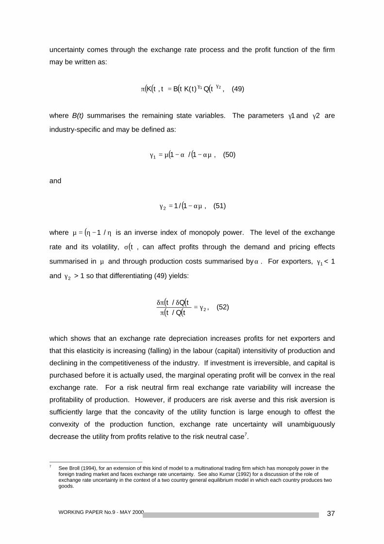
WORKING PAPER No.9 - MAY 2000 37
uncertainty comes through the exchange rate process and the profit function of the firm
may be written as:
( )( ) ( ) ( ) ,tQ)t(KtBt,tK 21 γγ=π (49)
where B(t) summarises the remaining state variables. The parameters 1γ and 2γ are
industry-specific and may be defined as:
( ) ( ),1/11 αµ−α−µ=γ (50)
and
( ),1/12 αµ−=γ (51)
where ( ) η−η=µ /1 is an inverse index of monopoly power. The level of the exchange
rate and its volatility, ( )tσ , can affect profits through the demand and pricing effects
summarised in µ and through production costs summarised byα . For exporters, 1γ < 1
and 2γ > 1 so that differentiating (49) yields:
( ) ( )( ) ( ) ,
tQ/ttQ/t
2γ=π
δδπ (52)
which shows that an exchange rate depreciation increases profits for net exporters and
that this elasticity is increasing (falling) in the labour (capital) intensitivity of production and
declining in the competitiveness of the industry. If investment is irreversible, and capital is
purchased before it is actually used, the marginal operating profit will be convex in the real
exchange rate. For a risk neutral firm real exchange rate variability will increase the
profitability of production. However, if producers are risk averse and this risk aversion is
sufficiently large that the concavity of the utility function is large enough to offest the
convexity of the production function, exchange rate uncertainty will unambiguously
decrease the utility from profits relative to the risk neutral case7.
7 See Broll (1994), for an extension of this kind of model to a multinational trading firm which has monopoly power in the
foreign trading market and faces exchange rate uncertainty. See also Kumar (1992) for a discussion of the role ofexchange rate uncertainty in the context of a two country general equilibrium model in which each country produces twogoods.
WORKING PAPER No.9 - MAY 200038
So exchange rate volatility is likely to have an ambiguous effect on international trade.
One way of recovering the traditional story of volatility on trade is to take a longer term
perspective of volatility, what De Grauwe (1988) labels the 'political economy of exchange
rate variability'. In particular, if exchange rate volatility persists over periods of months or
quarters then it is likely to lead to exchange rate misalignments which may have the kind of
consequences for output and employment referred to earlier. Of course these can be two
sided for the depreciated country their will be a stimulus to growth while in the appreciated
country growth worsens. The political economy idea is that in such a country individuals
organise themselves to pass different forms of protectionist legislation so that international
trade is negatively affected. The problem with this story is that volatility is a relatively high
frequency concept whereas the kind of effect that is being referred to here is more the
long-run / hysteresis effect on the real exchange rate and so it becomes difficult to
distinguish the volatility effect from the misalignment/ levels effect.
It is often thought that the existence of capital markets, and in particular forward markets,
should short-circuit the effects of exchange rate volatility on international trade. However,
hedging is costly, especially in periods when exchange rate volatility is high and, more
fundamentally, forward markets are notoriously incomplete - they may be relatively deep
for periods of up to a year but thereafter there are often important missing markets.
Indeed, a number of papers have demonstrated that the basic effects of exchange rate
volatility on trade are unchanged in the presence of capital markets (see, for example,
Demers (1991) and Viane and de Fries (1992)).
So in terms of the volatility effect the benefits of a country, or group of countries, moving
from flexible to fixed exchange rate are unclear, even although this move should reduce
such volatility to zero. However, it is worth emphasising that moving to a rigidly fixed set of
exchange rates, as in a monetary union, may in itself be trade enhancing. For example,
Mundell (1961) argued that the removal of a number of separate currencies and their
replacement with a single currency should facilitate and stimulate trade. Furthermore, the
adoption of a common currency by a nation state represents a very real commitment to
longterm integration and this could induce the private sector to engage in more trade
(Rose (2000)). Perhaps, also, the existence of a common currency in the eurozone area
will induce greater financial integration which, in turn, will produce more trade in goods and
services.
WORKING PAPER No.9 - MAY 2000 39
7.1.2 Evidence
From a theoretical perspective, the sign on the effect of exchange rate movements on
trade is ambiguous. Does the empirical literature shed any light on this issue? A number
of empirical studies have examined the influence of some measure of exchange rate
uncertainty - both real and nominal - on aggregate import and export volumes (see, inter
alia, Hooper and Kohlhagen (1978), Bailey, TavIas and Ulan (1986), Kenen and Rodrick
(1986), Caballero and Corbo (1989) and Chowdhury (1993)). These results are based on
standard trade equations, of the type introduced in our discussion of the H-M-K effect, with
the addition of some measure of exchange rate uncertainty (a variety of measures are
used in the literature ranging from the absolute percentage change of the exchange rate,
moving averages of the standard deviation to ARCH-based estimates)8. Usually an OLS
estimator, or variant of this estimator, is used in these papers and they do tend to confirm
the standard levels effect of the exchange rate on trade - a depreciation of the real
exchange rate increases trade volumes. However, there is no clear sign pattern on the
coefficient on the exchange rate uncertainty term: it is equally likely to be positive or
negative (furthermore few of the coefficients are significant). By its nature, however,
aggregate data may not be best-suited for testing the impact of exchange rate volatility on
trade because it implicitly assumes that the impact of exchange rate volatility is uniform
between countries and commodities in terms of direction and magnitude.
Indeed, it turns out that studies which have used disaggregate data have been much more
successful in achieving significant effects from the exchange rate uncertainy term. For
example, Cushman (1983) uses bilateral sectoral data spanning the period 1965-1977 for
a group of developed countries and finds statistically negative effects of his measure of
uncertainty on trade flows. In follow-up papers, Cushman (1986,1988) repeats this
exercise using data for the recent floating experience and does obtain clear evidence of a
statistically significant negative effect of volatility on trade flows. Cushman also reports a
small number of statistically positive coefficients. DeGrauwe (1987) uses bilateral
intra-EMS trade volume data and a period which encompasses both a pre-EMS period
(1973-78) and an EMS period. He demonstrated that for the EMS period exchange rates
were substantially less variable than non-participating countries and the more stable
exchange rate environment was more conducive to higher growth rates in international
trade.
8 See McKenzie (1999) for a survey of this literature.
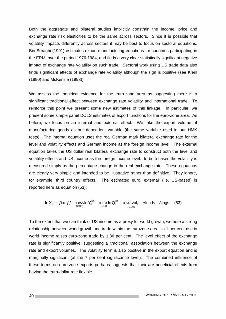
WORKING PAPER No.9 - MAY 200040
Both the aggregate and bilateral studies implicitly constrain the income, price and
exchange rate risk elasticities to be the same across sectors. Since it is possible that
volatility impacts differently across sectors it may be best to focus on sectoral equations.
Bin-Srnaghi (1991) estimates export manufactuting equations for countries participating in
the ERM, over the period 1976-1984, and finds a very clear statistically significant negative
impact of exchange rate volatility on such trade. Sectoral work using US trade data also
finds significant effects of exchange rate volatility although the sign is positive (see Klein
(1990) and McKenzie (1998)).
We assess the empirical evidence for the euro-zone area as suggesting there is a
significant traditional effect between exchange rate volatility and international trade. To
reinforce this point we present some new estimates of this linkage. In particular, we
present some simple panel DOLS estimates of export functions for the euro-zone area. As
before, we focus on an internal and external effect. We take the export volume of
manufacturing goods as our dependent variable (the same variable used in our HMK
tests). The internal equation uses the real German mark bilateral exchange rate for the
level and volatility effects and German income as the foreign income level. The external
equation takes the US dollar real bilateral exchange rate to construct both the level and
volatility effects and US income as the foreign income level. In both cases the volatility is
measured simply as the percentage change in the real exchange rate. These equations
are clearly very simple and intended to be illustrative rather than definitive. They ignore,
for example, third country effects. The estimated euro, external' (i.e. US-based) is
reported here as equation (53):
.lagsleadsvolQlnYlnƒƒixeƒXln)29.0(
itUSit
)04.0(
USit
)05.0(it 546.0184.0855.1 ∆+∆++++= (53)
To the extent that we can think of US income as a proxy for world growth, we note a strong
relationship between world growth and trade within the eurozone area - a 1 per cent rise in
world income raises euro-zone trade by 1.86 per cent. The level effect of the exchange
rate is significantly positive, suggesting a 'traditional' association between the exchange
rate and export volumes. The volatility term is also positive in the export equation and is
marginally significant (at the 7 per cent significance level). The combined influence of
these terms on euro-zone exports perhaps suggests that their are beneficial effects from
having the euro-dollar rate flexible.
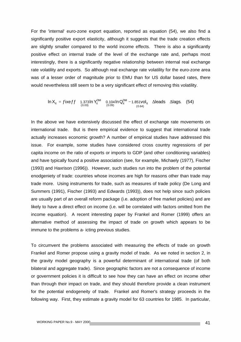
WORKING PAPER No.9 - MAY 2000 41
For the 'internal' euro-zone export equation, reported as equation (54), we also find a
significantly positive export elasticity, although it suggests that the trade creation effects
are slightly smaller compared to the world income effects. There is also a significantly
positive effect on internal trade of the level of the exchange rate and, perhaps most
interestingly, there is a significantly negative relationship between internal real exchange
rate volatility and exports. So although real exchange rate volatility for the euro-zone area
was of a lesser order of magnitude prior to EMU than for US dollar based rates, there
would nevertheless still seem to be a very significant effect of removing this volatility.
.lagsleadsvolQlnYlnƒƒixeƒXln)64.0(
itDMit
)09.0(
DMit
)03.0(it 851.1104.0373.1 ∆+∆+−++= (54)
In the above we have extensively discussed the effect of exchange rate movements on
international trade. But is there empirical evidence to suggest that international trade
actually increases economic growth? A number of empirical studies have addressed this
issue. For example, some studies have considered cross country regressions of per
capita income on the ratio of exports or imports to GDP (and other conditioning variables)
and have typically found a positive association (see, for example, Michaely (1977), Fischer
(1993) and Haxrison (1996)). However, such studies run into the problem of the potential
enodgeniety of trade: countries whose incomes are high for reasons other than trade may
trade more. Using instruments for trade, such as measures of trade policy (De Long and
Summers (1991), Fischer (1993) and Edwards (1993)), does not help since such policies
are usually part of an overall reform package (i.e. adoption of free market policies) and are
likely to have a direct effect on income (i.e. will be correlated with factors omitted from the
income equation). A recent interesting paper by Frankel and Romer (1999) offers an
alternative method of assessing the impact of trade on growth which appears to be
immune to the problems a- icting previous studies.
To circumvent the problems associated with measuring the effects of trade on growth
Frankel and Romer propose using a gravity model of trade. As we noted in section 2, in
the gravity model geography is a powerful determinant of international trade (of both
bilateral and aggregate trade). Since geographic factors are not a consequence of income
or government policies it is difficult to see how they can have an effect on income other
than through their impact on trade, and they should therefore provide a clean instrument
for the potential endogeneity of trade. Frankel and Romer's strategy proceeds in the
following way. First, they estimate a gravity model for 63 countries for 1985. In particular,
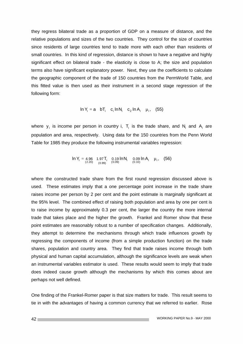
WORKING PAPER No.9 - MAY 200042
they regress bilateral trade as a proportion of GDP on a measure of distance, and the
relative populations and sizes of the two countries. They control for the size of countries
since residents of large countries tend to trade more with each other than residents of
small countries. In this kind of regression, distance is shown to have a negative and highly
significant effect on bilateral trade - the elasticity is close to A; the size and population
terms also have significant explanatory power. Next, they use the coefficients to calculate
the geographic component of the trade of 150 countries from the PermWorld Table, and
this fitted value is then used as their instrument in a second stage regression of the
following form:
,AlncNlncbTaYln ii2iiii µ++++= (55)
where iy is income per person in country i, iT is the trade share, and iN and iA are
population and area, respectively. Using data for the 150 countries from the Penn World
Table for 1985 they produce the following instrumental variables regression:
,AlnNlnTYln ii)10.0(
i)09.0()99.0(
i)20.2(
i 09.019.097.196.4 µ++++= (56)
where the constructed trade share from the first round regression discussed above is
used. These estimates imply that a one percentage point increase in the trade share
raises income per person by 2 per cent and the point estimate is marginally significant at
the 95% level. The combined effect of raising both population and area by one per cent is
to raise income by approximately 0.3 per cent, the larger the country the more internal
trade that takes place and the higher the growth. Frankel and Romer show that these
point estimates are reasonably robust to a number of specification changes. Additionally,
they attempt to determine the mechanisms through which trade influences growth by
regressing the components of income (from a simple production function) on the trade
shares, population and country area. They find that trade raises income through both
physical and human capital accumulation, although the significance levels are weak when
an instrumental variables estimator is used. These results would seem to imply that trade
does indeed cause growth although the mechanisms by which this comes about are
perhaps not well defined.
One finding of the Frankel-Romer paper is that size matters for trade. This result seems to
tie in with the advantages of having a common currency that we referred to earlier. Rose
WORKING PAPER No.9 - MAY 2000 43
(2000) also uses a version of the gravity model to try to unravel the relative effects that
exchange rate volatility and participation in a currency or monetary union can have on the
logarithm of bilateral trade. He uses a panel of 186 countries for five different years (1970,
1975, 1980, 1985 and 1990) and focuses on nominal measures of exchange rate volatility.
He finds that the coefficient on exchange rate volatility is around -0.017 and is statistically
significant at the 5% level. Reducing exchange rate volatility to zero from its sample mean
value of 5% would increase trade by approximately 8 per cent. However, the coefficient on
the currency union effect is 1.21 (and statistically significant), suggesting a much larger
effect on bilateral trade of 3.35 (i.e. 21.1e ); that is, countries with the same currency trade
over three times as much as with countries with different currencies. This result suggests
that the trade creating effects of participation in a currency union are likely to be very large.
For a number of reasons, however, the implications of this latter result for the euro-zone
area should be interpreted cautiously. For one thing, the panel constitutes a large number
of non-euro-zone participants and it is unclear, for example, if the categorisation of these
countries as participating in a monetary union is actually picking up this or, perhaps, the
effect of other institutional effects, such as common legal systems. Indeed, some of the
countries classed as members of a monetary union are not formally in a monetary union
but simply a fixed exchange rate arrangement. In fact only 1 per cent of the total number
of observations countries in the panel represent participants of a monetary union.
However, Rose's results are provocative and perhaps suggest an upper bound on what
the currency union point estimate is likely to be.
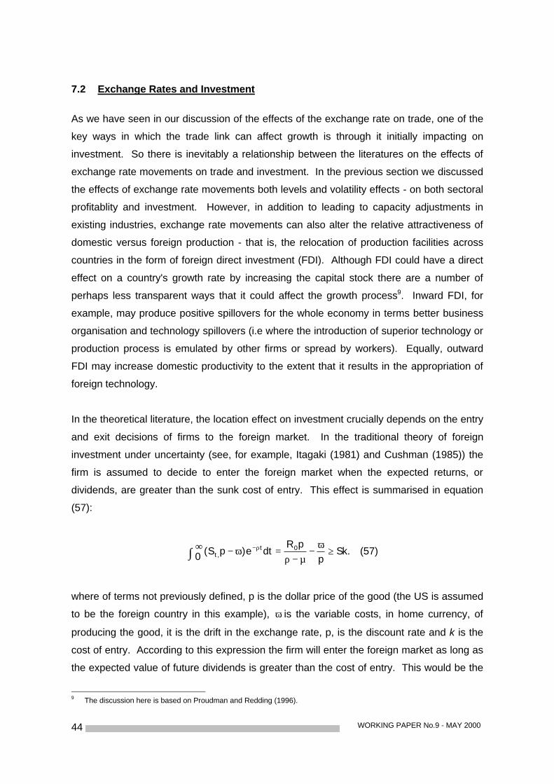
WORKING PAPER No.9 - MAY 200044
7.2 Exchange Rates and Investment
As we have seen in our discussion of the effects of the exchange rate on trade, one of the
key ways in which the trade link can affect growth is through it initially impacting on
investment. So there is inevitably a relationship between the literatures on the effects of
exchange rate movements on trade and investment. In the previous section we discussed
the effects of exchange rate movements both levels and volatility effects - on both sectoral
profitablity and investment. However, in addition to leading to capacity adjustments in
existing industries, exchange rate movements can also alter the relative attractiveness of
domestic versus foreign production - that is, the relocation of production facilities across
countries in the form of foreign direct investment (FDI). Although FDI could have a direct
effect on a country's growth rate by increasing the capital stock there are a number of
perhaps less transparent ways that it could affect the growth process9. Inward FDI, for
example, may produce positive spillovers for the whole economy in terms better business
organisation and technology spillovers (i.e where the introduction of superior technology or
production process is emulated by other firms or spread by workers). Equally, outward
FDI may increase domestic productivity to the extent that it results in the appropriation of
foreign technology.
In the theoretical literature, the location effect on investment crucially depends on the entry
and exit decisions of firms to the foreign market. In the traditional theory of foreign
investment under uncertainty (see, for example, Itagaki (1981) and Cushman (1985)) the
firm is assumed to decide to enter the foreign market when the expected returns, or
dividends, are greater than the sunk cost of entry. This effect is summarised in equation
(57):
.Skp
pRdte)pS(0
0t,t ≥
ω−
µ−ρ=ω−∞ ρ−∫ (57)
where of terms not previously defined, p is the dollar price of the good (the US is assumed
to be the foreign country in this example), ω is the variable costs, in home currency, of
producing the good, it is the drift in the exchange rate, p, is the discount rate and k is the
cost of entry. According to this expression the firm will enter the foreign market as long as
the expected value of future dividends is greater than the cost of entry. This would be the
9 The discussion here is based on Proudman and Redding (1996).
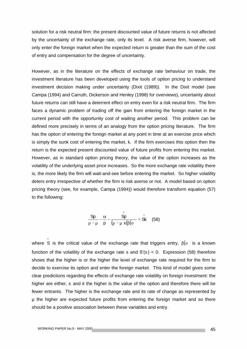
WORKING PAPER No.9 - MAY 2000 45
solution for a risk neutral firm: the present discounted value of future returns is not affected
by the uncertainty of the exchange rate, only its level. A risk averse firm, however, will
only enter the foreign market when the expected return is greater than the sum of the cost
of entry and compensation for the degree of uncertainty.
However, as in the literature on the effects of exchange rate behaviour on trade, the
investment literature has been developed using the tools of option pricing to understand
investment decision making under uncertainty (Dixit (1989)). In the Dixit model (see
Campa (1994) and Carruth, Dickerson and Henley (1998) for overviews), uncertainty about
future returns can still have a deterrent effect on entry even for a risk neutral firm. The firm
faces a dynamic problem of trading off the gain from entering the foreign market in the
current period with the opportunity cost of waiting another period. This problem can be
defined more precisely in terms of an analogy from the option pricing literature. The firm
has the option of entering the foreign market at any point in time at an exercise price which
is simply the sunk cost of entering the market, k. If the firm exercises this option then the
return is the expected present discounted value of future profits from entering this market.
However, as in standard option pricing theory, the value of the option increases as the
volatility of the underlying asset price increases. So the more exchange rate volatility there
is, the more likely the firm will wait-and-see before entering the market. So higher volatility
deters entry irrespective of whether the firm is risk averse or not. A model based on option
pricing theory (see, for example, Campa (1994)) would therefore transform equation (57)
to the following:
( ) ( )( )^
^
Skx
Spp
Sp=
σβµ−ρ−
ω−
µ−ρ (58)
where ^S is the critical value of the exchange rate that triggers entry, ( )σβ is a known
function of the volatility of the exchange rate s and ß'(s ) < 0. Expression (58) therefore
shows that the higher is or the higher the level of exchange rate required for the firm to
decide to exercise its option and enter the foreign market. This kind of model gives some
clear predictions regarding the effects of exchange rate volatility on foreign investment: the
higher are either, s and k the higher is the value of the option and therefore there will be
fewer entrants. The higher is the exchange rate and its rate of change as represented by
µ the higher are expected future profits from entering the foreign market and so there
should be a positive association between these variables and entry.
WORKING PAPER No.9 - MAY 200046
One final effect worth noting in the investment decision-making context is the affect of
portfolio or wealth effects (see Froot and Stein (1991) for an explicit model). For example,
a revaluation of the local currency makes home investors wealthier and this effect could
offset or reinforce the kind of investment effects referred to above. For example, changes
in the euro-dollar exhange rate will, through such revaluation effects, 'shift' portfolio wealth
between the US and the euro-zone area. Whether this leads to more home or foreign
investment will very much depend on the preferences of investors - in particular, if they
have a home or foreign bias. If investors have a foreign bias then an exchange rate
appreciation will lead to more investment in the foreign country.
Cushman (1985) uses a pooled cross sectional-time series analysis to examine the effects
of expectational and risk factors on FDI flows from the United States to Canada, Ranee,
Germany, Japan and the UK over the period 1963 to 1978 (annual observations). Various
expectations mechanisms - such as regressive and stabilising expectations - are used to
generate measures of the expected change in the real exchange rate. Real exchange rate
risk is defined as the standard deviation of the quarterly change in the real exchange rate.
In sum, Cushman finds that the level of the real exchange rate has a positive sign although
statistical significance is weak across specifications, the expected change in the real
exchange rate is significantly negative in all specifications and the risk term is positive
although the statistical significance is rather weak. The coefficient on the expected
exchange rate variable is largest, indicating that a 1 per cent change affects direct
investment flows in a given year by 19 to 28 per cent.
Froot and Stein (1991) examine the effects that the level of the exchange rate has on
aggregate and 13 disaggregate components of foreign direct investment (FDI) into the US
(sample period 1974-1987, annual). They find a statistically significant negative
relationship between all of the FDI components and the level of the real effective exchange
rate. They additionally regress Ms for Canada, Japan, the UK, West Germany, on the
level of the relevant real effective exchange rate and a constant. All of the coefficients on
the level of the exchange rates are negative, apart from Canada, although only the
coefficient in the West German equation is statistically significant. Froot and Stein use the
kind of wealth effect referred to above to argue that a weak dollar, with imperfect capital
markets, increases the relative wealth of foreign investors compared to home investors
(US) and will therefore increase the attractiveness of investments in the US.
WORKING PAPER No.9 - MAY 2000 47
Goldberg (1994) examines the effects of the volatility and level of the real exchange rate
(and other control variables) for aggregate and disaggregate US investment for the period
1970 quarter 1 through to 1989 quarter IV10. Although she finds very little evidence of
exchange rate effects on the aggregate measures of investment, there is some evidence
to suggest that it is important for disaggregate measures. For example, it is shown that in
the 1980s dollar depreciations (appreciations) reduced (stimulated) investment in
manufacturing nondurables sectors and had mixed effects in nonmanufacturing sectors.
Goldberg argues that this result could arise if the portfolio/ wealth effects of exchange
rates oil investment dominate the demand effect for traded goods and the production
effects. This result tends to conflict with the standard argument in favour of having a
depreciated exchange rate. Exchange rate volatility is shown to have resulted in a
contraction of investment in some sectors of US industry in the 1980s but these effects are
small. She argues that this is consistent with the model of risk averse investors,
irreversibilities of investment and profit convexities in the presence of imperfect
competition discussed in the previous section.
Using a panel data set based of 6I US wholesale trade industries for the period 198I to
1987, Campa (1994) examines the effects of exchange rate volatility and the level of the
exchange rate on entry of firms into the US market. The literature on foreign investment
has shown that the effect of the exchange rate on investment depends on where the good
is produced, the national source of the inputs used in production and the country where the
final good is sold. To avoid these complications, Campa focuses on entry in the wholesale
trade industries in the US by foreign manufacturing companies. The reduced form
estimated is based on (58):
.,k,,S,ƒn t
ωσµ=−−+−+
(59)
The dependent variable is the number of firms that entered an industry in a given year and
µ and σ are the average and standard deviation of the monthly change of the exchange
rate. Since µ and σ embody the firms expectations of the future levels of these variables
there will in general be no unique assumption about how firms form these expectations.
Campa makes two assumptions: static expectations, in which the firms take the exchange
rate behaviour in the two years previous to entry, and perfect foresight expectations in
10 It is worth that this kind of test could be picking up the combined effect of what we have called the trade induced effects
of exchange rate changes and also the locational effects.
WORKING PAPER No.9 - MAY 200048
which the expost value for the next two years is used. Sunk costs are estimated using two
variables: the ratio of fixed assets to net wealth of all US firms in an industry and the ratio
of media expenditures to company sales by all US firms in each area. The measure of the
variable costs abroad, ω , is taken as a weighted average of the annual cross country
index of unit labour costs, where US has a value of 1. Since the right hand side variable is
a limited dependent variable, a Tobit estimator is used. To summarise the findings:
exchange rate volatility has a significantly negative effect on the numbers of firms entering
the industry. Both sunk costs and the level of advertising costs are found to be deterrents
to entry. The level of the exchange rate has a significantly positive effect on the entry
level. This latter results conflicts with the findings of Froot and Stein (1991) and Goldberg
(1994), although it is not necessarily inconsistent since this study focuses on the number
of entrants rather than the level of foreign direct investment. The empirical estimates also
reveal that interaction between sunk costs and the exchange rate is significant.
In sum, the extant empirical evidence on the effects of exchange rate movements on FDI
suggests that exchange rate volatility has a significantly negative effect. The empirically
estimated levels effect is ambiguous, although the balance of evidence seems to suggest
an opposite effect to that found in the trade literature and this may perhaps be explained
by appealing to a wealth effect.
Proudman and Redding (1998), summarising a number of research papers produced by
the Bank of England, analyse the effect of openness on growth in the UK economy for the
period 1970-92. Their measures of openness encompass trade factors, discussed in the
last section, and also FDI. In summary, their main empirical findings are: at the industry
sector level, average rates of sectoral productivity are positively correlated with a number
of measures of openness. Using discriminant analysis to classify sectors as relatively
open or closed, they find that open sectors have higher average growth rates of total factor
productivity than closed sectors. Over the sample period their estimate of the average
long-run rate of productivity in UK manufactures, relative to the US, rose from 58% to 69%
and around one-half of this increase was estimated to be due to openness. The openness
measures that are most important in explaining this increase are due to flows of goods and
indeas, rather than the flow of capital. Furthermore, it would seem that it is technological
change that is the main driving force behind the result and not specialisation due to
comparative advantage.
WORKING PAPER No.9 - MAY 2000 49
8. CONCLUSIONS
Exchange rates when flexible are highly volatile, and nominal exchange rate movements
can impart a considerable degree of persistence into real exchange rates. These are two
of the so-called stylised facts we discussed in Section 2 of this paper. In terms of the
euro-zone area, we have tried to distinguish the implications of such behaviour for both
internal and external exchange rates. What are the advantages and disadvantages of
fixing the level of the internal nominal exchange rate? First, the unpleasant consequences
of an appreciation of the nominal rate generating an uncompetitive real rate of one
participating country vis-à-vis its euro-zone competitors is ruled out. This would seem to
be a particular problem at the moment for the UK economy relative to its EU trading
partners. To set against this, however, there is the advantage of having some flexibility in
the exchange rates if business cycles are nonsynchronised across trading partners.
Although there is some evidence to suggest that this may indeed be the case within
Europe, it is our contention that both exchange rate unification and the single market
project are likely to make this less of an issue in the future. Also, the danger in having
some exchange rate flexibility within a free trade area is that it will be abused by countries
pursuing competitive beggarthy-neighbour type policies, and these policies are, at best,
likely to amount to a zero sum game. The second advantage of fixing internal exchange
rates within Europe is that it squeezes out the unpleasant consequences of exchange rate
volatility for trade and investment. Although the theoretical evidence is actually ambiguous
regarding the effect that such volatility should have on trade and investment, our reading of
the empirical evidence suggests that it is significantly negative for the countries
participating in the euro-zone project and therefore there must be real welfare gains, both
static and dynamic, from locking these currencies.
In terms of the external euro exchange rate, some of the arguments used above to justify
locking internal exchange rates may be used in reverse to argue for some flexibility in the
euro. We have noted, for example, that euro-zone exchange rates, as an entity, exhibit
mean-reverting behaviour and this implies that the real value of the euro can potentially
move to adjust external imbalances and also to assist if business cycle movements are
non-synchronous between the euro block and her trading partners. Our empirical
estimates suggest that there is a significant levels effect of the real exchange rate on
euro-zone trade and some economic commentators have argued that around
three-quarters of euro-zone growth in the current year is likely to emanate from the
external consequences of the depreciated value of the euro. Since the euro-zone area is a
WORKING PAPER No.9 - MAY 200050
relatively closed economy it is unlikely that volatility in the external value of the euro will
have much effect on inward investment and external euro-zone trade and, indeed, our
empirical estimates seem to confirm this.
An additional theme in this paper has been the effects of growth, particularly productivity
growth, on real exchange rates. We have argued that there does seem to be evidence
which suggests that Balassa-Samuelson type effects are statistically important for
euro-zone members and this will necessarily have implications for the behaviour of internal
real exchange rates, or inflation differentials, and real interest differentials between
member states. However, although these inflation differentials are likely to be important in
the short to medium run, as countries which were relatively slow growing prior to EMU
'catch-up', it seems unlikely that these differentials are inconsistent with the operation of a
monetary union. They may, however, prove problematic for countries seeking to
participate in monetary union, such as countries currently in the accession stages of EMU.
We have also examined the implications of the differential overall growth rates (as
opposed to just productivity growth) for the intra euro-zone real exchange rates and also in
terms of the euro-zone against the dollar. A standard partial equilibrium analysis of the
current account suggests that a country growing fast relative to its trading partners may
have to incur a secular depreciation in its real exchange rate. However, it has been noted
by a number of researchers that this need not occur if the ratio of the country's income
elasticity of exports to its income elasticity of imports equals the ratio of its growth to
foreign growth. A number of researchers have in fact demonstrated that this kind of
relationship - the 45° rule - holds pretty well for a period from the 1950's through to the
1970's. We have presented updated estimates of the 45° rule for the 1980s and 1990's,
with a particular emphasis on the euro-zone countries. We find that the rule holds pretty
tightly, on average, both in terms of internal euro-zone real exchange rates and also for the
external value of the euro. Indeed, the latter estimates suggests that the euro dollar rate
should have appreciated since its inception, although, of course, the 45° rule ignores the
implications of the capital account of the balance of payments for exchange rate
movements.
In sum, the current exchange rate arrangements in the euro-zone area are we believe
beneficial for both business cycle related growth and also longer run, or permanent,
growth. As always, the empirical estimates presented in this paper could be refined and
checked for robustness. It seems unlikely, however, that such extensions will change the

WORKING PAPER No.9 - MAY 2000 51
main conclusion of this paper: irrevocably fixing internal exchange rates, and having some
flexibility in the external value of the euro, will enhance the growth prospects of the
euro-zone area.
WORKING PAPER No.9 - MAY 200052
9. REFERENCES
Alberola, E. and Tyrvainen (1998), "Is there scope for inflation differentials in EMU? An
empirical evaluation of the Balassa-Samuelson model in EMU countries", Bank of Finland
Discussion Papers 15198, Bank of Finland.
Artus, JR. (1983), "Toward a more orderly exchange rate system, Finance and
Development, 20, 10-13.
Bailey, M., TavIas, G.S., and Ulan, M. (1986), "Exchange rate variability and trade
performance: Evidence for the big seven industrial countries, Weltwirschaftliches Archiv,
122, 466-77.
Balassa, B. (1964), "The Purchasing Power Parity Doctrine: A Reappraisal, Journal of
Political Economy, 72, 584-596.
Bayourni, T. and R. MacDonald (1999), "Deviations of Exchange Rates from Purchasing
Power Parity: A Story Featuring Two Monetary Unions", IMF Staff Papers.
Beveridge, Steven, and Charles R. Nelson, (1981), "A New Approach to the
Decomposition of Economic Time Series Into Permanent and Transitory Components, with
Particular Attention to the Measurement of Business Cycles", Journal of Monetary
Economics, Vol. 7, pp. 151-74.
Bhagwati, J. (1958), " Immiserizing growth: A geometrical note", Review of Economic
Studies, 25, 201-205.
Bhagwati, J. (1969), "International trade and economic expansion". In Trade, Tariffs and
Growth, Cambridge: MIT Press.
Bini-Srnaghi, L. (1991), "Exchange rate variability and trade: why is it so difficult to find
any relationship?" Applied Economics, 23, 927-36.
WORKING PAPER No.9 - MAY 2000 53
Bordo, M. and A. Schwartz (1999), "Policy Regimes and Economic Performance: The
Historical Record", in J. Taylor and M. Woodford (eds), Handbook of Macroeconomics.
Amsterdam: North-Holland
Brodsky, D. A. (1984), "Fixed versus flexible exchange rates and the measurement of
exchange rate instability", Journal of International Economics, 16, 295-306.
Broll, U. (1994), "Foreign production and forward exchange markets", Australian
Economic Papers, 62, 1-6.
Caballero, R.J. and V. Corbo (1989), "The effect of real exchange rate uncertainty on
exports: empirical evidence", The World Bank Economic Review, 3, 263-278.
Campa, J.M. (1993), "Entry by foreign firms in the United States under exchange rate
uncertainty", Review of Economics and Statistics, LXXV, 614622..
Canzoneri, M.B., R.E. Cumby and B. Diba (1996), "Relative Productivity and the Real
Exchange Rate in the Long Run: Evidence for a Panel of OECD Countries", CEPR
Discussion Paper No. 1464.
Canzoneri, M.B., R.E. Cumby and Eudy (1996), "Trends in European productivity and real
exchange rates: implications for the Maastricht convergence criteria and for inflation
targets after emu, CEPR Discussion Paper, No 1417.
Carruth, A. A. Dickerson and A. Henley (1998), "What do we know about investment
under uncertainty?", University of Kent, Working paper No., 98/4.
Chinn, M. (1997), " Sectoral Productivity, Government Spending and Real Exchange
Rates: Empirical Evidence for OECD Countries", in R. MacDonald and J. Stein (eds),
Equilibrium Exchange Rates, Amsterdam: Kluwer.
Chinn, M. and L. Johnston (1996), "Real Exchange Rate Level, Productivity and demand
Shocks: Evidence from a Panel of 14 Countries", NBER Discussion paper No 5709.
Chowdhury, A.R. (1993), "Does exchange rate volatility depress tarde flows? evidence
from error correction models", Review of Economics and Statistics, 75, 700-6.
WORKING PAPER No.9 - MAY 200054
Clarida, R. and J. Cali (1995), "Sources of Real Exchange Rate Fluctuations: How
Important are Nominal Shocks?", Carnegie-Rochester Series on Public Policy, 41, 1-56
Clark, P.B. and R. MacDonald, (1998), "Exchange Rates and Economic Fundamentals: A
Methodological Comparison of BEERs and FEERs" in R. MacDonald and J. Stein (eds),
Equilibrium Exchange Rates, Amsterdam: Kluwer.
Cushman, D. (1983), " The effects of exchange rate risk on international trade", Journal of
International Economics, 15, 45-63.
Cushman, D. (1986), " Has exchange risk depressed international trade: the impact of
third country international trade", Journal of International Money and Finance, 5, 361-79.
Cushman, D. (1988), "US bilateral trade flows and exchange risk during the floating
period", Journal of International Economics, 24, 317-30.
De Grauwe, P. (1987) "International trade and economic growth in the european monetary
system", European Economic Review, 31, 389-98.
De Grauwe, P. (1988), "Exchange rate variability and the slowdown in the growth of
international trade", IMF Staff Papers, 35, 63-85.
De Long, B.J. and L. Summers (1991), "Equipment, Investment and Economic Growth",
Quarterly Journal of Economics, 106, 445-502.
Demers, M. (1991), "Investment under uncertainty, irreversibility and the arrival of
information over time, Review of Economic Studies, 58, 333-50.
Dixit, A.K. (1989), "Hysteresis, Import Penetration, and Exchange Rate Pass Through",
Quarterly Journal of Economics, 104, 205~228.
Dornbusch, Rudiger, (1976) "Expectations and Exchange Rate Dynamics", Journal of
Political Economy, Vol. 84, pp. 1161-76.
WORKING PAPER No.9 - MAY 2000 55
Engel, C. (1993) "Real Exchange Rates and Relative Prices: An Empirical Investigation",
Journal of Monetary Economics, 32, 35-50.
Engel, C. and J.11. Rogers (1996), "How Wide is the Border?", American Economic
Review, Vol. 86, 1112-1125
Ethier, W. (1973), "International trade and the foreign exchange market", American
Economic Review, 63, 494-503.
Fischer, S. (1993), "The role of macroeconomic factors in growth", Journal of Monetary
Economics, 32, 485-512.
Flood, R. and A. Rose, (1999) "Understanding exchange rate volatility without the
contrivance of macroeconomics", Economic Journal, 109, F660-F672.
Franke, G. (1991), "Exchange rate volatility and international trade strategy, Journal of
International Money and Finance, 10, 292-307.
Frankel, J. (1979), "On the Mark: A Theory of Floating Exchange Rates Based on Real
Interest Differentials", American Economic Review, 69, 610-22.
Frankel, J and A. Rose (1995) "A Panel Project on Purchasing Power Parity: Mean
Reversion Within and Between Countries", NBER Working Paper No. 5006 (Cambridge,
Massachusetts: National Bureau of Economic Research.
Frankel, J. and D. Romer (1999), "Does trade cause growthT' American Economic
Review, 379-399
Frenkel, J. and M. Mussa, (1986) "Asset Markets, Exchange Rates, and the Balance of
Payments", Chapter 14 in E. Grossman and K. Rogoff (eds) Handbook of International
Economics, Vol. 2 Amsterdam: North Holland.
Froot, K. and J Stein (199 1), "Exchange rates and foreign direct investment% Quarterly
Journal of Economics, 106, 1191-1218.
WORKING PAPER No.9 - MAY 200056
Ghosh, A.R., A. Gulde, 1D Ostrey and H Wolf (1995), "Does the nominal exchange rate
matter, IMF Working Paper, 121.
Goldberg, L. (1993), "Exchange rates and investment in United States industry", Review
of Economics and Statistics, LXXV, 575-588.
Group of Ten (1985), "The Functioning of the International Monetary System", Report by
the Deputies of the Group of Ten, Washington DC.
Group of Twenty Four (1985), "The Functioning and Imprivement of the Inetrnational
Monetary Sysyetm", Report by the Deputies of the Group of Twenty Four.Washington DC.
Harrison, A. (1996), "Openness and growth: a time series cross-country analysis for
developing countries", Journal of Development Economics, 48, 41947.
Hoffinarm M. and R. MacDonald (2000), "A real differential view of real exchange rates",
mimeo, University of Strathclyde.
Hooper, P. and S. Kohlhagen (1978), "The effect of exchange rate uncertainty on the
price and volume of international trade", Journal of International Economics 8, 483-511.
Houthakker, H. and S. Magee (1969), "Income and Price Elasticities in World Trade,
Review of Economics and Statistics, 51, 111-125.
Johnson, H. (1958), International Trade and Economic Growth: Studies in Pure Theory,
London: Allen and Unwin.
Juselius, K. (1995), 'Do purchasing power parity and uncovered interest rate parity hold in
the long run? An example of likelihood inference in a multivariate time-series model'
Journal of Econometrics, 69, 211-240.
Kao, C. (1999), "Spurious regression and residual-based tests for cointegration in panel
data", Journal of Econometrics, 90, 1-44.
Kenen, P. and D. Rodrick (1986), "Measuring and Analysisng the effects of short-term
volatility on real exchange rates, Review of Economics and Statistics, 71, 708-12.
WORKING PAPER No.9 - MAY 2000 57
Kohler, M. (1999), "The Balassa-Samuelson Effect and Monetary Tragets", mimeo, Bank
of England.
Krugman, P. (1989), "Differences in Income Elasticities and 'kends in Real Exchange
Rates, European Economic Review, 33, 1031-1054.
Kumar, V. (1992), "Real effects of exchange risk on international trade", working paper
92-5, Fegeral Reserve Bank of Australia.
La Cour, L. and R. MacDonald (2000), "Modelling the ECU-US Dollar Exchange Rate: A
Structural Monetary Interpretation", Journal of Business Economics and Statistics,
forthcoming.
Levin A. and C-F Lin (1994), "Unit root tests in panel data: Asymptotic and finite-sample
properties", mimeo, Federal Reserve Board.
Lucas, R. (1982), "Interest rates and currency prices in a two-country world" Journal of
Monetary Economics, 10, 335-60.
MacDonald, R. (1993) "Long-Run Purchasing Power Parity: Is It for Real7 Review of
Economics and Statistics, Vol. 75, pp. 690-5.
MacDonald, R. (1995) "Long-Run Exchange Rate Modeling: A Survey of the Recent
Evidence" Staff Papers, International Monetary Fund, Vol. 42, 3, 437-489.
MacDonald, R. (1999b), "Exchange Rates: Do Fundamentals Matter?", Economic Journal,
109, F673-17691
MacDonald, R.(2000), Exchange Rate Economics: Theories and Evidence, second edition,
London: Routledge Keegan Paul.
MacDonald, R. and LW. Marsh (1997), "On Casselian PPP, Cointegration and Exchange
Rate Forecasting" Review of Economics and Statistics, November,
WORKING PAPER No.9 - MAY 200058
MacDonald, R. and L Ricci (2000), 'Deviations from Purchasing Power Parity: Does the
Distribution Sector Make a Difference?", forthcoming IMF working paper.
MacDonald, R. and P. Swagel (1998), "Real Exchange Rates and the Business Cycle"
forthcoming as IMF Working Paper.
McKenzie, M.D. (1999), "The impact of exchange rate volatility on international trade
flows", Journal of Economic Surveys, 13, 71-106.
Mark, N. and D. Sul (1999), A computationally simple cointegration vector estimator for
panel data", mimeo, Ohio State University.
Michaely, M. (1977), "Exports and growth: An empirical investigation", Journal of
Development Economics, 4, 49-53.
Mundell, R. (1961), "A theory of optimum currency areas", American Economic Review,
Mussa, M. (1978), "Empirical regularities in the behaviour of exchange rates and theories
of the foreign exchange market", in Carnegie-Rochester Series on Publci Policy, Vol 11,
9-57
Officer, Lawrence H., (1976), "The Purchasing Power Parity Theory of Exchange Rates: A
Review Article", Staff Papers, International Monetary Fund, Vol. 23, pp. 1-60.
Proudman, J. and S. Redding (1998), "The relationship between openness and growth in
the United Kingdom: a summary of the Bank of England Openness and Growth ProjecC,
Bank of England Quarterly Bulletin, 390-405.
Rogers J.H. and M Jenkins (1995), "Haircuts or hysteresis" sources of movements in real
exchange rates", Journal of International Economics, 38, 339-360.
Rose, A. (2000) "One money, one market: the effect of common currencies on trade"
Economic Policy, 9-45
Samuelson, P. (1964), "Theoretical Problems on Trade Problems", Review of Economics
and Statistics, 46, 145-154.
WORKING PAPER No.9 - MAY 2000 59
Stock, J.H. and M Watson (1993), "A simple estimator of cointegrating vectors in higher
order integrated systems", Econometrica, 61: 783-820.
Stockman, A. (1987), "The Equilibrium Approach to Exchange Rates", Federal Reserve
Bank of Richmond Economic Review,
Stockman, A. (1988), "Real Exchange Rate Variability Under Pegged and Floating
Nominal Exchange Rate Systems: An Equilibrium Theory", Carnegie Rochester
Conference Series on Public Policy, 29: 259-294.
Stockman, A. (1995), "Sources of Real Exchange-Rate Fluctuations: A Comment,
Carnegie Rochester Conference Series on Public Policy, 41, 57-65.
Viaene, J.M. and C.G de Vries (1992), "International trade and exchaneg rate volatility%
European Economic Review, 36, 1311-21.
Weber, A. (1997), "Sources of Purchasing Power Disparities between the G3 Economies",
Journal of Japanese and International Economies, 11, 548-583.
Wei, S-J and D. Parsley (1995), "Purchasing Power Disparity during the Recent Floating
Rate Period: Exchange Rate Volatility, Trade Barriers and Other Culprits", Quarterly
Journal of Economics.
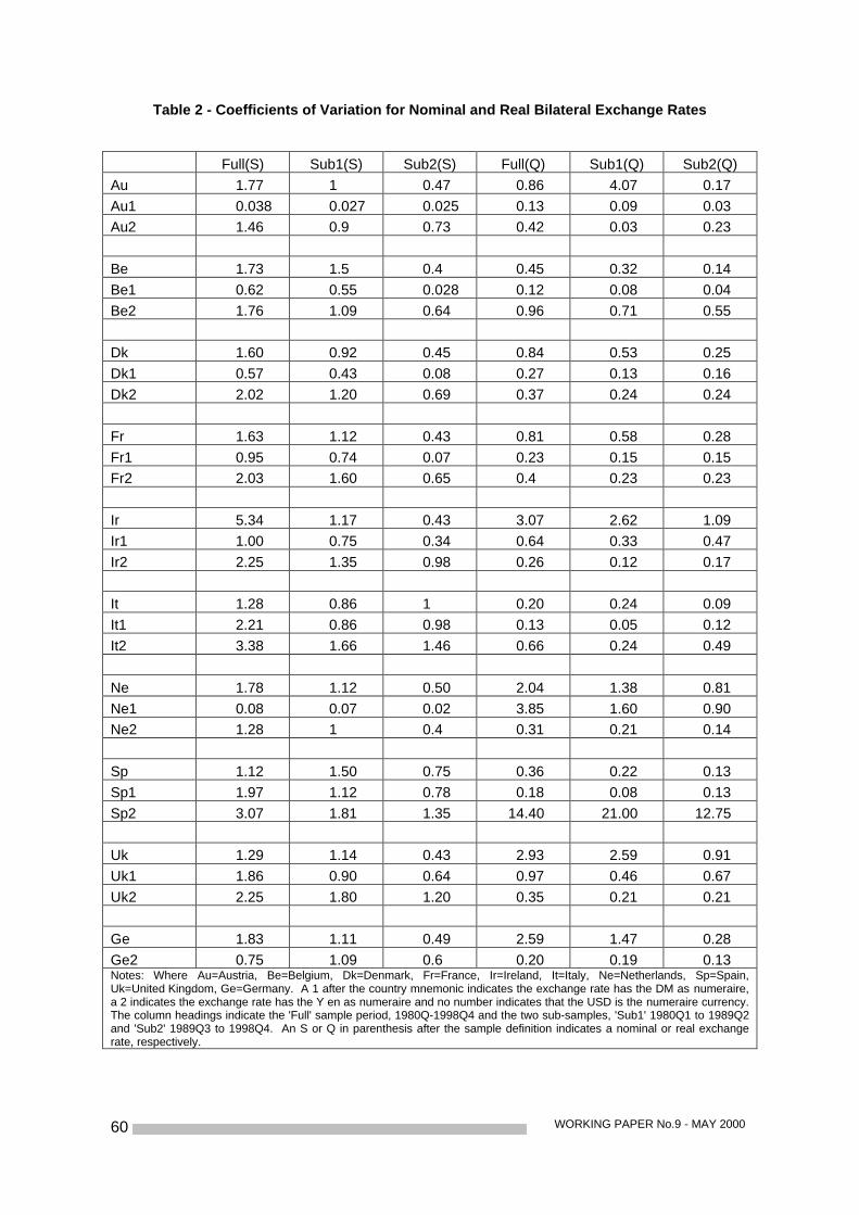
WORKING PAPER No.9 - MAY 200060
Table 2 - Coefficients of Variation for Nominal and Real Bilateral Exchange Rates
Full(S) Sub1(S) Sub2(S) Full(Q) Sub1(Q) Sub2(Q)Au 1.77 1 0.47 0.86 4.07 0.17Au1 0.038 0.027 0.025 0.13 0.09 0.03Au2 1.46 0.9 0.73 0.42 0.03 0.23
Be 1.73 1.5 0.4 0.45 0.32 0.14Be1 0.62 0.55 0.028 0.12 0.08 0.04Be2 1.76 1.09 0.64 0.96 0.71 0.55
Dk 1.60 0.92 0.45 0.84 0.53 0.25Dk1 0.57 0.43 0.08 0.27 0.13 0.16Dk2 2.02 1.20 0.69 0.37 0.24 0.24
Fr 1.63 1.12 0.43 0.81 0.58 0.28Fr1 0.95 0.74 0.07 0.23 0.15 0.15Fr2 2.03 1.60 0.65 0.4 0.23 0.23
Ir 5.34 1.17 0.43 3.07 2.62 1.09Ir1 1.00 0.75 0.34 0.64 0.33 0.47Ir2 2.25 1.35 0.98 0.26 0.12 0.17
It 1.28 0.86 1 0.20 0.24 0.09It1 2.21 0.86 0.98 0.13 0.05 0.12It2 3.38 1.66 1.46 0.66 0.24 0.49
Ne 1.78 1.12 0.50 2.04 1.38 0.81Ne1 0.08 0.07 0.02 3.85 1.60 0.90Ne2 1.28 1 0.4 0.31 0.21 0.14
Sp 1.12 1.50 0.75 0.36 0.22 0.13Sp1 1.97 1.12 0.78 0.18 0.08 0.13Sp2 3.07 1.81 1.35 14.40 21.00 12.75
Uk 1.29 1.14 0.43 2.93 2.59 0.91Uk1 1.86 0.90 0.64 0.97 0.46 0.67Uk2 2.25 1.80 1.20 0.35 0.21 0.21
Ge 1.83 1.11 0.49 2.59 1.47 0.28Ge2 0.75 1.09 0.6 0.20 0.19 0.13Notes: Where Au=Austria, Be=Belgium, Dk=Denmark, Fr=France, Ir=Ireland, It=Italy, Ne=Netherlands, Sp=Spain,Uk=United Kingdom, Ge=Germany. A 1 after the country mnemonic indicates the exchange rate has the DM as numeraire,a 2 indicates the exchange rate has the Y en as numeraire and no number indicates that the USD is the numeraire currency.The column headings indicate the 'Full' sample period, 1980Q-1998Q4 and the two sub-samples, 'Sub1' 1980Q1 to 1989Q2and 'Sub2' 1989Q3 to 1998Q4. An S or Q in parenthesis after the sample definition indicates a nominal or real exchangerate, respectively.
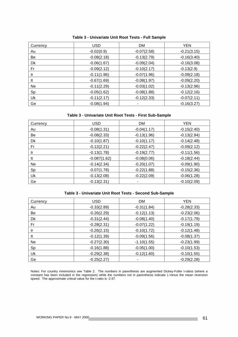
WORKING PAPER No.9 - MAY 2000 61
Table 3 - Univariate Unit Root Tests - Full Sample
Currency USD DM YENAu -0.02(0.9) -0.07(2.58) -0.21(3.15)Be -0.08(2.18) -0.13(2.79) -0.16(3.40)Dk -0.06(1.67) -0.09(2.04) -0.16(3.08)Fr -0.09(2.12) -0.10(2.17) -0.13(2.9)Ir -0.11(1.96) -0.07(1.96) -0.09(2.18)It -0.67(1.69) -0.08(1.97) -0.09(2.20)Ne -0.11(2.29) -0.03(1.02) -0.13(2.96)Sp -0.05(1.62) -0.08(1.88) -0.12(2.16)Uk -0.11(2.17) -0.12(2.33) -0.07(2.11)Ge -0.08(1.94) - -0.16(3.27)
Table 3 - Univariate Unit Root Tests - First Sub-Sample
Currency USD DM YENAu -0.08(1.31) -0.04(1.17) -0.15(2.40)Be -0.08(2.33) -0.13(1.96) -0.13(2.94)Dk -0.10(1.87) -0.10(1.17) -0.14(2.48)Fr -0.12(2.21) -0.22(2.47) -0.09(2.12)Ir -0.13(1.78) -0.19(2.77) -0.11(1.56)It -0.087(1.62) -0.08(0.06) -0.18(2.44)Ne -0.14(2.34) -0.20(1.07) -0.09(1.90)Sp -0.07(1.78) -0.22(1.88) -0.15(2.36)Uk -0.13(2.08) -0.22(2.09) -0.06(1.28)Ge -0.13(2.31) - -0.10(2.09)
Table 3 - Univariate Unit Root Tests - Second Sub-Sample
Currency USD DM YENAu -0.33(2.89) -0.31(1.84) -0.28(2.33)Be -0.26(2.29) -0.12(1.13) -0.23(2.06)Dk -0.31(2.44) -0.08(1.40) -0.17(1.79)Fr -0.28(2.31) -0.07(1.22) -0.19(1.19)Ir -0.26(2.15) -0.10(1.72) -0.12(1.48)It -0.12(1.39) -0.09(1.56) -0.08(1.37)Ne -0.27(2.30) -1.10(1.55) -0.23(1.99)Sp -0.16(1.88) -0.05(1.00) -0.10(1.53)Uk -0.29(2.38) -0.12(1.60) -0.10(1.55)Ge -0.25(2.27) - -0.29(2.28)
Notes: For country mnemonics see Table 2. The numbers in parenthesis are augmented Dickey-Fuller t-ratios (where aconstant has been included in the regression) while the numbers not in parenthesis indicate 1 minus the mean reversionspeed. The approximate critical value for the t-ratio is -2.97.
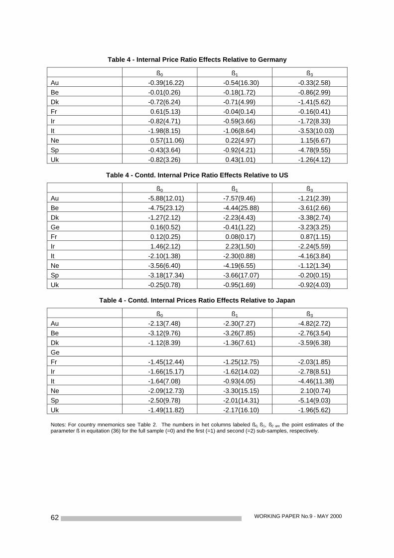
WORKING PAPER No.9 - MAY 200062
Table 4 - Internal Price Ratio Effects Relative to Germany
ß0 ß1 ß3
Au -0.39(16.22) -0.54(16.30) -0.33(2.58)Be -0.01(0.26) -0.18(1.72) -0.86(2.99)Dk -0.72(6.24) -0.71(4.99) -1.41(5.62)Fr 0.61(5.13) -0.04(0.14) -0.16(0.41)Ir -0.82(4.71) -0.59(3.66) -1.72(8.33)It -1.98(8.15) -1.06(8.64) -3.53(10.03)Ne 0.57(11.06) 0.22(4.97) 1.15(6.67)Sp -0.43(3.64) -0.92(4.21) -4.78(9.55)Uk -0.82(3.26) 0.43(1.01) -1.26(4.12)
Table 4 - Contd. Internal Price Ratio Effects Relative to US
ß0 ß1 ß3
Au -5.88(12.01) -7.57(9.46) -1.21(2.39)Be -4.75(23.12) -4.44(25.88) -3.61(2.66)Dk -1.27(2.12) -2.23(4.43) -3.38(2.74)Ge 0.16(0.52) -0.41(1.22) -3.23(3.25)Fr 0.12(0.25) 0.08(0.17) 0.87(1.15)Ir 1.46(2.12) 2.23(1.50) -2.24(5.59)It -2.10(1.38) -2.30(0.88) -4.16(3.84)Ne -3.56(6.40) -4.19(6.55) -1.12(1.34)Sp -3.18(17.34) -3.66(17.07) -0.20(0.15)Uk -0.25(0.78) -0.95(1.69) -0.92(4.03)
Table 4 - Contd. Internal Prices Ratio Effects Relative to Japan
ß0 ß1 ß3
Au -2.13(7.48) -2.30(7.27) -4.82(2.72)Be -3.12(9.76) -3.26(7.85) -2.76(3.54)Dk -1.12(8.39) -1.36(7.61) -3.59(6.38)GeFr -1.45(12.44) -1.25(12.75) -2.03(1.85)Ir -1.66(15.17) -1.62(14.02) -2.78(8.51)It -1.64(7.08) -0.93(4.05) -4.46(11.38)Ne -2.09(12.73) -3.30(15.15) 2.10(0.74)Sp -2.50(9.78) -2.01(14.31) -5.14(9.03)Uk -1.49(11.82) -2.17(16.10) -1.96(5.62)
Notes: For country mnemonics see Table 2. The numbers in het columns labeled ß0, ß1, ß2 are the point estimates of theparameter ß in equitation (36) for the full sample (=0) and the first (=1) and second (=2) sub-samples, respectively.
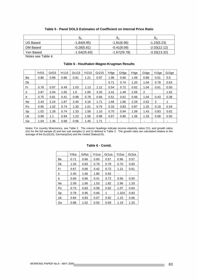
WORKING PAPER No.9 - MAY 2000 63
Table 5 - Panel DOLS Estimates of Coefficient on Internal Price Ratio
ß0 ß1 ß3
US Based -1.84(9.95) -1.81(6.96) -1.23(5.23)DM Based -0.28(5.81) -0.41(8.09) -2.03(12.12)Yen Based -1.54(25.63) -1.67(29.78) -3.33(13.32)Notes see Table 4.
Table 6 - Houthaker-Magee-Krugman Results
Yrf15 Grf15 Yr115 Gr115 Yr215 Gr215 Yrfge Grfge Yrlge Grlge Yr2ge Gr2ge
Be 0.86 0.89 0.86 0.81 1.21 0.97 1.96 0.66 1.09 0.88 0.51 0.5
Dk 0.71 0.74 1.20 1.04 0.78 0.63
Fr 0.78 0.97 0.49 1.03 1.13 1.12 0.54 0.72 0.62 1.04 0.61 0.50
Ir 2.87 2.04 1.65 1.6 1.00 3.25 2.41 1.49 2.56 2 1.62
It 0.75 0.81 0.41 0.98 0.78 0.66 0.51 0.61 0.66 1.04 0.43 0.38
Ne 2.43 2.24 1.87 2.40 4.16 1.71 1.66 1.66 2.29 2.62 2 1
Po 0.95 1.02 0.74 1.30 1.01 0.75 0.33 0.83 0.87 1.25 0.19 0.34
Sp 1.02 1.28 0.74 1.33 1.58 1.10 0.70 0.94 1.09 1.43 0.83 0.62
Uk 0.98 1.1 0.94 1.23 1.56 0.98 0.67 0.80 1.06 1.33 0.68 0.50
Ge 1.04 1.36 0.68 0.96 1.45 1.71 - - - - - -
Notes: For country Mnemonics, see Table 2. The column headings indicate income elasticity ratios (Yr), and growth ratios(Gr) for the full sample (f) and two sub samples (1 and 2) defined in Table 2. The growth rates are calculated relative to theaverage of the Eu15(15), Germany(Ge) and the United States(US).
Table 6 - Contd.
Yrfus Grfus Yr1us Gr1us Yr2us Gr2us
Be 0.71 0.66 0.60 0.57 0.96 0.57
Dk 1.03 0.83 0.79 0.78 0.70 0.83
Fr 0.67 0.66 0.42 0.72 1.21 0.61
Ir 2.40 1.66 1.80 0.92 - -
It 0.60 0.66 0.41 0.72 0.56 0.50
Ne 2.09 1.66 1.53 1.82 2.96 1.33
Po 0.73 0.83 0.58 0.92 1.07 0.64
Sp 0.78 0.95 0.66 1 1.324 0.83
Uk 0.84 0.83 0.67 0.92 1.15 0.66
Ge 0.88 1.02 0.50 0.69 1.19 1.33
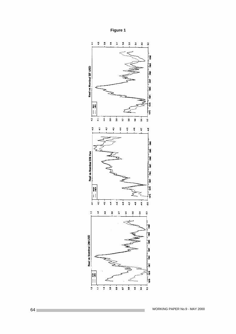
WORKING PAPER No.9 - MAY 200064
Figure 1
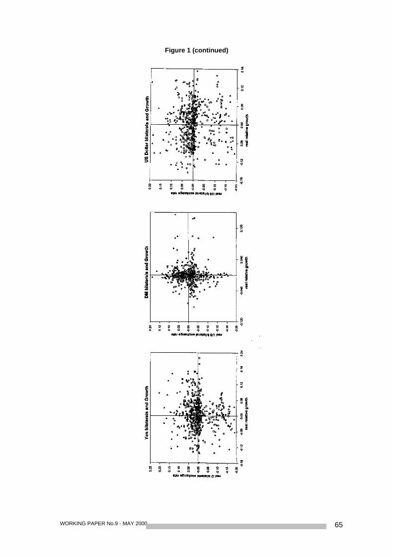
WORKING PAPER No.9 - MAY 2000 65
Figure 1 (continued)
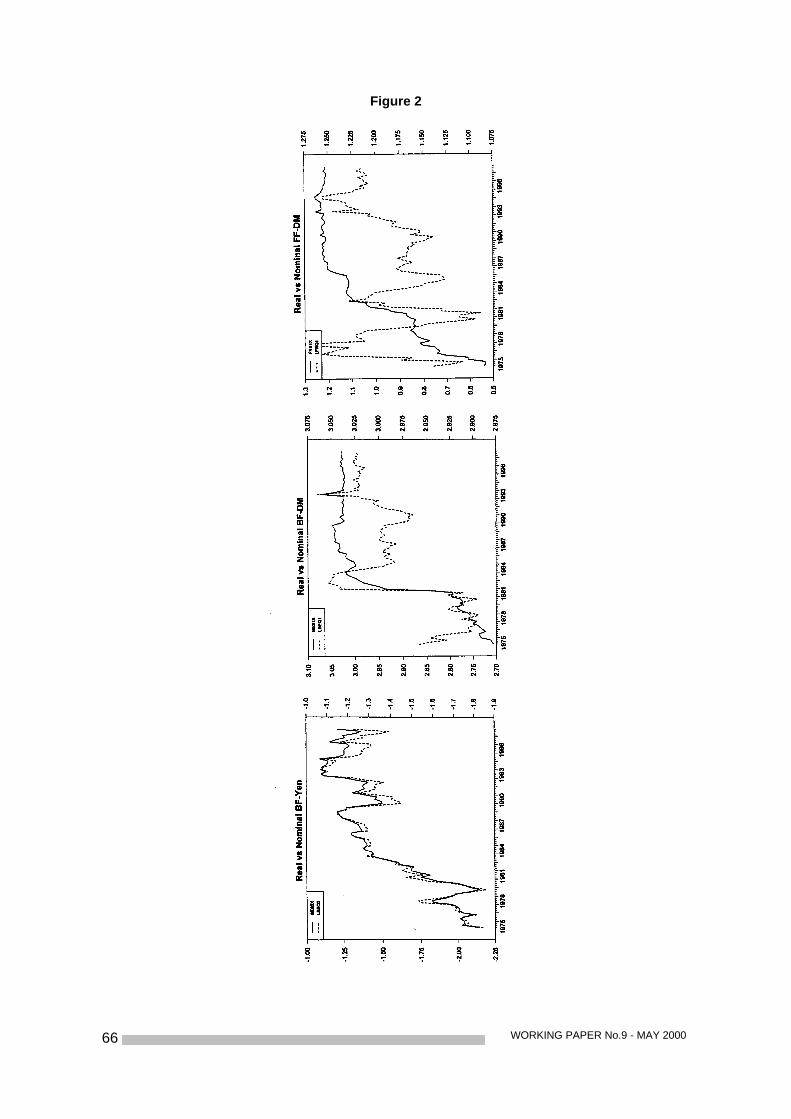
WORKING PAPER No.9 - MAY 200066
Figure 2
WORKING PAPER No.9 - MAY 2000 67
NATIONAL BANK OF BELGIUM - WORKING PAPERS SERIES
1. "Model-based inflation forecasts and monetary policy rules" by M. Dombrecht and R. Wouters,
Research Series, March 2000
2. "The use of robust estimators as measures of core inflation" by L. Aucremanne, Research
Series, March 2000
3. "Performances économiques des Etats-Unis dans les années nonante" by A. Nyssens, P.
Butzen, P. Bisciari, Document Series, March 2000.
4. "A model with explicit expectations for Belgium" by P. Jeanfils, Research Series, March 2000.
5. "Growth in an open economy: some recent developments" by S. Turnovsky, Research Series,
May 2000
6. "Knowledge, technology and economic growth: an OECD perspective" by I. Visco, Research
Series, May 2000
7. "Fiscal policy and growth in the context of European integration" by P. Masson, Research
Series, May 2000
8. "Economic growth and the labor markets: Europe's challenge" by C. Wyplosz, Research
Series, May 2000
9. "The role of the exchange rate in economic growth" by R. MacDonald, Research Series, May
2000
10. "Economic growth and monetary union" by J. Vickers, Research Series, May 2000