The Role of Training Programs for Youth Employment in Nepal: Impact

Evaluation Report on the Employment Fund1

October 2014

Ali Ahmed, Shubha Chakravarty2, Mattias Lundberg and Plamen Nikolov

Abstract

The youth unemployment rate is exceptionally high in the developing world. Because quality of education is

arguably one of the most important determinants of youth’s labor force participation, governments worldwide have

responded by creating job training and placement services programs. Despite the rapid expansion of skill-

enhancement employment programs across the world and the long history of training program evaluations, debates

about the causal impact of training based labor market policies on employment outcomes still persist.

Using a quasi-experimental approach, this report presents the short-term effects of skills training and employment

placement services in Nepal. Launched in 2009, the intervention provided skills training and employment placement

services for over 40,000 Nepalese youth over a three-year period, including a specialized adolescent girls’ initiative

that reached 4410 women aged 16 to 24. We find, approximately two years into the program, the EF intervention

positively improved employment outcomes. EF training program participation generated an increase in non-farm

employment of 16 to17 percentage points for an overall gain of 47 percent. The program also generated an average

monthly earnings gain by about 45 percent for the 2010 cohort. These impacts were driven by female participants,

and younger women aged 16 to 24 experienced the same improvements as older females. These employment

estimates are comparable, though higher, than other recent experimental interventions in developing countries.

1 Acknowledgments

Many individuals and organizations provided support for this ongoing research. Chiefly, the Employment Fund and its staff have

championed this study for several years, offering their time, resources, and data to the research team, the survey firm, and

administrators of other programs under the Bank’s Adolescent Girls Initiative. Mr. Siroco Messerli and Bal Ram Paudel, (Team

Leaders), in particular, have facilitated all aspects of the study, including liaising with the T&E providers. We would like to thank

the T&E providers for allowing unrestricted access and support to the survey team.

The Employment Fund is supported through the generous financial support of the Swiss Development Corporation (SDC), and

the UK’s Department for International Development (DFID). This research study has benefited from the financial support of the

World Bank’s Multi-donor Trust Fund for Adolescent Girls and DFID. The field surveys were led by New Era Limited, which

provided exceptional survey design and implementation, data management and analysis under the leadership of Mr. Madhup

Dhungana.

On behalf of the World Bank, the project implementation was led by Jasmine Rajbhandary, Venkatesh Sundararaman, and

Bhuvan Bhatnagar. Amita Kulkarni, Uttam Sharma and Jay Krishna Upadhaya coordinated survey activities in the field in 2010

and 2011, 2012 respectively. Marine Gassier and Jennifer Heintz of the World Bank provided excellent research assistance.

2 Correspondence should be sent to: schakravarty@worldbank.org

Table of Contents

I. Introduction ........................................................................................................................................... 1

II. The Adolescent Girls Initiative ............................................................................................................. 4

a. Programs worldwide ......................................................................................................................... 4

b. The Employment Fund and the Adolescent Girls Employment Initiative (AGEI) in Nepal ............ 5

III. Impact Evaluation Design ................................................................................................................. 8

IV. Methodology and Data .................................................................................................................... 10

a. Sample Description and Sampling Technique ................................................................................ 10

b. Estimating the EF Training Program Effects .................................................................................. 13

c. Intent-to-Treat (ITT) and Average Treatment Effect on the Treated (ATT) .................................. 16

d. Heterogeneous Effects .................................................................................................................... 17

V. Internal Validity .................................................................................................................................. 18

a. Pre-existing time-varying trends ..................................................................................................... 18

b. Survey response rates and attrition ................................................................................................. 19

c. Uptake of EF-sponsored training courses ....................................................................................... 20

VI. Short-Run Results of the EF Program ............................................................................................. 21

a. First-stage Estimation of Propensity Scores ................................................................................... 21

b. Impacts on Employment and Earnings for the Full Sample ........................................................... 22

c. Non-Employment Impacts for the Full Sample .............................................................................. 25

d. Trade-wise Program Impacts on the Full Sample ........................................................................... 27

e. Gender-disaggregated Impacts ........................................................................................................ 28

VII. Summary and Implications ............................................................................................................. 30

VIII. REFERENCES ............................................................................................................................... 33

Annex 1. Figures and Tables. ................................................................................................................... 37

Annex 2. Example Ranking Form ........................................................................................................... 53

Annex 3. Analysis of Average Treatment Effects on the Treated (ATT) Impacts .............................. 54

1

I. Introduction

Youth unemployment and underemployment across much of the developing world is extremely

high. Two facts highlight the importance of youth’s labor in the world economy: 17 percent of

the world’s population are youth (ages 16-24) and youth make up 40 percent of the world’s

unemployed.3

In developing countries, where labor frequently encompasses informal self-employment and

small scale agriculture, youth also struggle with high underemployment (they are not able to

work as much as they would like to) and low productivity. In 2010, 536 million of employed

youth in developing countries were underemployed, compared to 1.5 million in the 27 European

Union (EU) countries.4 Youth unemployment and underemployment not only slow down

economic growth but also negatively impact crime rates (Fella and Gallipoli, 2007), depression

rates (Frese and Mohr, 1987), substance abuse rates (Linn, Sandifer and Stein, 1985), and rates

of social exclusion (Goldsmith, Veum and Darity, 1997).

Nepal is similarly affected by youth unemployment and underemployment. With a per capita

income of US$700, Nepal is South Asia’s second poorest country (ahead of only Afghanistan).

Helped by remittances, the proportion of the population falling below the national poverty line

has declined in recent years from 31 percent in 2003-04 to 25 percent in 2011 (Central Bureau of

Statistics 2011). One underlying factor of poverty in Nepal is the lack of employment

opportunities, and a reliance on self-employment in the agriculture sector, which accounts for 61

percent of the total labor force (Nepal Living Standard Survey 2011). The unemployment rate for

those aged 15-29 is 19.2 percent, compared to just 2.7 percent for people older than 15 (ILO

2014). Faced with these prospects, young Nepalese are compelled to consider migrating overseas

in search of better opportunities.

Governments worldwide have responded by creating job training and placement services

programs. In 2013, European Union (EU) launched an eight billion initiative aiming to provide

every young European with a job, apprenticeship, or training within four months of becoming

3 See http://www.weforum.org/community/global-agenda-councils/youth-unemployment-visualization-2013 4 See http://www.weforum.org/community/global-agenda-councils/youth-unemployment-visualization-2013

2

unemployed.5 In Latin America, job training programs (referred to collectively as the “Jovenes”

programs) have been implemented since the early 2000s. To date, more than 700 youth

employment programs from around 100 countries have been implemented and more than 80

percent of these programs offer some sort of skills training.6

Despite the rapid expansion of skill-enhancement employment programs across the world and

the long history of training programs’ evaluations7, debates about the causal impact of training

based labor market policies on employment outcomes still persist. Based on US and European

evidence, Card et al. (2009) review impacts of various training programs. Their analysis suggests

that classroom and on-the-job training programs are not particularly effective in the short run,

but have larger positive impacts after two years. They also find that youth programs, on average,

tend to yield less positive impacts than untargeted programs. The evidence regarding impacts by

gender is mixed. Kluve (2006) reviewed a number of employment program evaluations in

Europe and found that the programs tended to have larger impacts for women than men.

However, Card (2009), found that programs tended to work equally well for men and women.

In general, program evaluations from developing countries show larger impacts than programs

conducted in other regions. Based on 289 youth employment interventions in 84 countries,

Betcherman et al. (2007) show higher impact in developing countries than in developed ones.8

Most of the rigorous evidence on training programs in developing countries is from Latin

America, where positive impacts are particularly pronounced (Gozalez et al., 2012; Attanasio et

al., 2008).9 Attanasio et al. (2008) evaluate the Jovenes en Acción job training program in

Colombia. Jovenes en Acción provided three months of classroom training followed by a three

month unpaid internship at a company. Attanasio et al. (2008) detect positive employment

effects for women (4 to 7 percentage points), no employment effects for men and positive

earnings effects for both men (8 percent) and women (18 percent). The study argues that the

5See http://www.economist.com/news/leaders/21582006-german-led-plans-tackling-youth-unemployment-europe-are-far-too-

timid-guaranteed-fail and http://www.dw.de/the-lost-generation-youth-unemployment-in-the-eu/a-16925070 6 See http://www.youth-employment-inventory.org/ 7 See Heckman (1999) and many others, including randomized controlled trials, like the Job Training Partnership Act in the US. 8 Betcherman et al. (2007) also found that only one-quarter of the 289 studies reviewed included an experimental or quasi-

experimental design. Among this particular subset of studies, 40 percent showed zero or negative impact on employment and

earnings outcomes. Betcherman et al. (2007) concludes that observational studies were almost 50 percent more likely to exhibit

positive impacts than programs with experimental or quasi-experimental designs. 9 Only Card et al. (2007) detects no statistically significant effect. Card et al. (2007) evaluate a job training program in the

Dominican Republic which included classroom training and a private sector internship. The impact evaluation shows no effect on

employment and a marginally significant earnings effect of about 10%.

3

increase in earnings is due to increased employment in formal sector jobs upon training

completion.10

In Nepal, a wide variety of public and private technical education and vocational training

(TEVT) programs are available to youth. Youth unemployment is frequently cited as a driver of

the ten-year conflict from which Nepal emerged in 2006 (Macours 2011, ILO 2014), and since

then international donors have invested heavily in the TEVT sector. Additionally, a combination

of age, low educational attainment, and norms around marriage and childbirth confers multiple

additional disadvantages to young women in the labor market. Their labor force participation rate

is 43.0 percent compared to 51.7 percent for young men (ILO 2014). Concerns about the social

exclusion of women, ethnic minorities, indigenous peoples, and other historically disadvantaged

groups have also spurred advocacy and investment in training opportunities for these groups. The

sector remains fragmented, however, with many public, private, and non-governmental training

providers of varying quality and weak links to the job market. To the best of our knowledge, no

rigorous evidence yet exists on the impacts of these programs on the labor market outcomes of

participants.

Using a quasi-experimental approach, this report presents the short-term effects of skills training

and employment placement services in Nepal. Founded in 2008, the Employment Fund (EF) is

operated by Helvetas, a Swiss NGO, in partnership with the Government of Nepal. It is currently

one of the largest youth training initiatives in the country, serving almost 15,000 youth annually.

In partnership with the Employment Fund’s donors,11

the Adolescent Girls Employment

Initiative (AGEI) was launched in 2009 to expand the program’s reach to an additional 4,410

Nepali women aged 16-24 over a three-year period.

Unique characteristics of this impact evaluation include:

A large study sample (3142 individuals in the 2010 and 2011 cohorts examined in this

report)

Particular focus on the outcomes of women aged 16-24 as well as the outcomes of a

broader category of youth (men and women aged 16-35)

10 Two previous evaluations of Jovenes-type programs in Argentina and Peru similarly found larger impacts for women than for

men, with employment impacts for women of 9 to 12 percentage points in Argentina (Aedo et. al. 2004) and 6 to 15 percentage

points in Peru (Ñopo et. al. 2007). 11 The Employment Fund is financed by the United Kingdom’s Department for International Development (DFID), the Swiss

Agency for Development and Cooperation (SDC) and the World Bank.

4

Socio-economic survey data of participants and a control group of non-participants as

well as administrative follow-up data of program participants

Exhaustive tracking of program participants over time that produced high response rates.

Examination of a large set of outcome domains, including employment and earnings,

empowerment and self-confidence, risky behaviors, and impacts on the household.

We find, approximately two years into the program, the EF program positively improved

employment outcomes. EF training program participation generated an increase in non-farm

employment of 16-17 percentage points for an overall gain of 47 percent. The program also

generated an average monthly earnings gain of 650-750 NRs monthly (8-9 USD). Given that

the average monthly income at baseline was 1428 NRs ( 19 USD), the EF program impact

generated an economically meaningful income gain of about 45 percent for the 2010 cohort.

These impacts were driven by the program’s female participants. For men enrolled in the EF

training program, we detect no statistically significant short-run impacts of the EF program on

employment or earnings. We detect no difference in impacts when comparing older (24-35) and

younger women (age 16-24), indicating that the program is equally effective for the younger

women targeted under the AGEI.

This report’s employment estimates are comparable, though slightly higher, than other recent

experimental interventions in developing countries. Estimates of employment increase by

Attanasio et al. (2008) and Alzua et al. (2013) show respectively a gain of 14 percentage points

10 percentage points. In terms of earnings, this intervention stands in stark contrast in that its

estimate is considerably higher than the increase in earnings of 18 percent gain estimates by

Attanasio et al. (2008).

The report is organized as follows: In Section II, we describe the global Adolescent Girls

Initiative and the Employment Fund program in Nepal. Section III describes the design of the

AGEI impact evaluation, Section IV describes our empirical approach, and Section V discusses

the potential threats to the study’s validity. Section VI presents results and Section VII

concludes.

II. The Adolescent Girls Initiative

a. Programs worldwide

5

Aiming to facilitate the transition to productive employment for young females, The World Bank

and its partners launched the Adolescent Girls Initiative (AGI) in 2009. Comprised of eight pilot

projects – in Afghanistan, Haiti, Jordan, Laos, Liberia, Nepal, Rwanda and South Sudan– the

initiative’s launch was motivated by two factors: (1) the particular challenges faced by young

women in developing countries during the school-to-work transition, including high burden of

domestic work, competing pressures to bear and raise children, negative social norms regarding

occupational choice and mobility, gender discrimination, and (2) the potential benefits -- to

household members, and to current and future children -- of empowering young women.

AGI interventions offered skills training and various ancillary services tailored to local

context, such as childcare, mentoring, job placement assistance, and links to microcredit, in order

to facilitate young women’s transition to productive employment. Six of the eight pilots included

an experimental component and two of the impact evaluations have reported results. Using a

randomized evaluation, the AGI project in Jordan provided short-term soft-skills training and

six-month employment vouchers to recent female graduates of technical universities. Although

the vouchers assisted young women to obtain short-terms internships, the evaluation detected no

effect on the recipients’ employment or earnings after the end of the voucher period (Groh,

2010). In contrast, the AGI pilot in Liberia found strong positive impacts on employment and

earnings. Based on a randomized “pipeline” design, individuals were randomly assigned to

receive training in two sequential batches. In addition to positive impacts on participants’ self-

confidence, savings, and household food security, the program had sizable impacts on

employment (47 percent) and weekly earnings (80 percent) for women aged 16-27 (Adoho

2014). Finally, a related project implemented by the international NGO BRAC in Uganda

implemented village-level girls’ clubs to provide life skills, reproductive health, and livelihood

skills to young women aged 14 to 20. A randomized impact evaluation found substantial

increases in employment (72 percent) and improved empowerment and reproductive health

outcomes (Bandiera 2012).

b. The Employment Fund and the Adolescent Girls Employment Initiative

(AGEI) in Nepal

Started in 2008, the Employment Fund (EF), now one of the largest skills training programs in

the country, provides vocational training and placement services under a unique governance

structure. Since 2011, the Employment Fund has operated under an agreement between the

Government of Nepal and Swiss Agency for Development and Cooperation (SDC). A Steering

6

Committee, chaired by the Joint Secretary of the Ministry of Education, governs the

Employment Fund. In addition to providing training and placement services, the Employment

Fund engages in support activities, capacity-building, and cooperative activities with the

Government’s Council for Technical Education and Vocational Training (CTEVT).

Each year, the Employment Fund authorizes training programs under a competitive bidding

system with various training providers. First, the Employment Fund issues a call for proposals to

Training and Employment (T&E) providers seeking to provide skills training and employment

services. The range of T&E provider types is enormous: from formal technical and vocational

training (TVET) institutions, public and private providers, to skilled artisans offering

apprenticeships. The second step, after the call for proposals, is for each T&E provider to

complete a Rapid Market Assessment (RMA) outlining viable and potential employment

opportunities.12

The third step in the process is for the EF to evaluate submitted proposals

according to preset criteria; the EF weighs the capacity and experience of each T&E provider,

the market demand for the proposed trades being offered, and the proposed costs. Finally, the EF

issues a contract to selected providers: the contract specifies the number of training courses

(hereafter called “events”) to be conducted and the number of individuals to be trained and

employed in each event. The T&E providers are then free to recruit and select their own trainees

for each of their training events, according to guidelines established by EF.

Table 1 provides the total number of T&E providers, number of training events, and number of

trainees. Table 1 shows an increase of total number of program beneficiaries between 2010 and

2011. Training courses in technical skills vary across a wide range of trades (e.g., incense stick

rolling, carpentry, tailoring, welding and masonry). All females receive 40 hours of life skills

training (beginning in 2011) and a sub-set of EF trainees receive a short course in basic business

skills. In addition, each trainee is encouraged to complete a skills certification test offered by the

National Skills Testing Board (NSTB).13

Upon completion of the classroom-based training, the EF places emphasis on job placement

services. EF verifies trainees’ employment status three months and six months after the

completion of the training.14

Upon verification, T&E providers receive an outcome-based

12 The RMA process is facilitated via EF-supported capacity building workshops. 13 In some cases, the Employment Fund has even cooperated with the NSTB to develop skills standards for tests in trades where

no test existed. 14 The employment status of a sample of graduates is verified by EF field monitors three to six months after the completion of the

training event.

7

payment from the EF that is higher for trainees who are employed. The outcome-based payment

system creates strong incentives for the T&E providers to provide placement assistance and

provides graduates with an opportunity to put their new skills to work immediately after the

training. The EF emphasizes the placement of trainees into “gainful” employment in which they

earn a minimum of 3,000 NRs (40 USD) per month.15

In 2010, the EF partnered with DFID and the World Bank’s Adolescent Girls Initiative to

improve the EF’s reach and impact for young women aged 16-24. Training under this

Adolescent Girls Employment Initiative (AGEI) proceeded in the same way as it did for other EF

trainees, except that certain events had been flagged in advance as likely to attract female

trainees. This was done in order to ensure that the EF reached adequate numbers of young

women.16

For the purpose of this evaluation, we designate all female participants aged 16-24 in

EF-sponsored training courses as “AGEI”.

The Employment Fund struggled in 2010 to recruit young women to training events and in 2011

launched an enhanced communication and outreach strategy to recruit more female trainees.17

. In

addition to the T&E advertisement, the EF sponsored radio and newspaper ads specifically

geared towards young women. Many of these ads specifically encouraged women to sign up for

non-traditional trades for women, such as mobile phone repair, electronics, or construction.18

The

Employment Fund also partnered with women’s and community-based organizations to attract

applications from women and marginalized groups – if a referred applicant gained entry to an

EF-sponsored training event, the partner organization was paid a small finder’s fee equivalent to

about 1.25 US dollar per person.

The Employment Fund uses a differential pricing mechanism that awards a higher incentive to

service providers who agree to train (and place) more disadvantaged groups, according to

established vulnerability criteria.19

The highest incentive is awarded for training and placing the

15 The definition of “gainful” employment was increased in 2012 to 4,600 NRs (60 USD). Throughout this report, we use the

prevailing exchange rate during 2010 and 2011 of 75 NRS to 1 USD. 16 The T&E providers running these training events are not given hard quotas for how many AGEI trainees to reach, but any

female trainees aged 16 to 24 that they do train are designated as “AGEI” trainees for accounting and monitoring purposes.

Employment Fund records indicate that 4410 young women were reached over the three year initiative, as shown in Table 1,

exceeding the target of 4375. 17 They reached only a bit more than half of their annual target of 1500. 18Anecdotal evidence also suggests that the introduction of life skills training, covering topics such as communication, leadership,

and reproductive health, was particularly popular among young women and may have contributed to the growing numbers of

AGEI trainees. 19 For more details on the differential pricing scheme for vulnerable groups and the outcome-based payment system, see

http://www-

8

most disadvantaged (highly vulnerable women including AGEI trainees, widows, ex-combatants,

disabled women, etc.), and incentives are gradually lowered for less prioritized groups. Training

providers that are able to cater to these higher priority target groups are therefore eligible to

receive a higher outcome price, but they also face a higher risk of failing to achieve the outcome

(gainful employment). The combination of a results-based system with a progressive incentive

scheme ensures that training providers with the capacity to work with vulnerable groups will

likely opt to do so.

III. Impact Evaluation Design

This evaluation estimates the impact of the EF training program by comparing the outcomes of

participants, who comprise the “treatment” group, to a control group of individuals who applied,

but were not selected for, an EF-sponsored training course. Isolating the causal effects of the EF

training program on employment and other outcomes is complicated by the fact that some T&E

providers have at least some degree of choice over who they choose to train or training

participants could seek EF training for reasons we cannot fully measure.20

In other words,

comparing post-program participation outcomes of EF program participants versus non-

participants may confound training program influences on outcomes with those of hard-to-

measure individual-level, family-level or T&E-level attributes that affect both training program

participation and the outcome of interest.

This estimation problem would be greatly reduced if we could compare the outcomes of

individuals from truly comparable backgrounds except for their EF training program status. The

primary concern in being able to detect the causal effects of the training program is that the two

sets of individuals (i.e., ones receiving training and ones who do not) may have had different

characteristics to begin with and it may be those characteristics rather than the EF training

program that explain the difference in outcomes between the two groups.21,22

The unobserved

differences in characteristics are particularly concerning.

wds.worldbank.org/external/default/WDSContentServer/WDSP/IB/2014/07/18/000470435_20140718142756/Rendered/PDF/894

760BRI0141100Box385283B00PUBLIC0.pdf 20 Systematic differences in unobservable characteristics that cannot be measured quantitatively, such as motivation, confidence,

and natural ability, will lead to biased estimates of program impact. 21 We perform a number of statistical tests (presented in section 5) to examine the similarities and differences between the two

groups in our evaluation sample. 22 The difference-in-differences method helps resolve this problem to the extent that many characteristics of units or individuals

can reasonably be assumed to be constant over time (or time-invariant). Think, for example, of observed characteristics, such as a

person’s year of birth, a region’s location close to the ocean, a town’s level of economic development, or a father’s level of

education. Most of these types of variables, although plausibly related to outcomes, will probably not change over the course of

9

T&E providers can select beneficiaries into their training programs, a process that drives the

difference between trainees and non-trainees. Each T&E provider advertises, collects

applications, shortlists and interviews applicants, and selects participants for each of training

events following Trainee Selection guidelines established by EF. These guidelines stipulate a

two week minimum period of advertisement, the eligibility criteria for training events, and the

procedures for shortlisting and interviewing. There are three eligibility criteria for all EF-

sponsored training programs: age (from 16 to 35), education (below SLC,23

or less than 10 years

of formal education), and self-reported economic status.24

Only applicants who meet all three

criteria are eligible to be shortlisted. T&E providers are advised to shortlist at least 50 percent

more candidates than the number of spaces in the training event. The guidelines also outline a

uniform process for interviewing shortlisted candidates, including a detailed scoring rubric,

instructions for ranking the shortlisted candidates by score, and selecting the top-scoring

candidates for participation.25

Figure 1 in Annex 2 shows a sample ranking form used by T&E

providers. This scoring and ranking procedure forms the basis of our sampling strategy for this

evaluation and is described in detail in the next section.

We use quasi-experimental methods to solve the above evaluation concerns and we attempt to

isolate the causal effects of EF training with:

(1) A difference-in-difference (DID) technique, and

(2) A difference-in-difference technique in combination with a propensity score matching

(PSM).

an evaluation. Using the same reasoning, we might conclude that many unobserved characteristics of individuals are also more or

less constant over time. 23 The School Leaving Certificate (SLC) is obtained after successfully passing examinations after the 10th grade. To be eligible,

EF applicants must have not taken, or not passed, their SLC exams. This criterion has been loosened for some trades starting in

2012. In practice, because the educational status reported on the application is not verified, this criterion was not perfectly

adhered to. 24An applicant is considered “economically poor” if they report a non-farm per capita household income of less than 3000 Nepali

rupees (NRs) per month or, in the case of farming families, less than 6 months of food sufficiency. Since these self-reports are

not verified, and applicants know in advance that they must be “poor” in order to be eligible for the program, it is unclear how

well this criterion is adhered to. 25 In addition, and as mentioned earlier, the guidelines also set out a progressive payment structure to incentivize T&E providers

to select trainees from particular socially disadvantage groups. The guidelines also allow for T&E providers to select up to 2

“alternates” per event, in case a selected trainee declines to join the program.

10

Conceptually, the difference-in-differences method (Campbell, 1969; Meyer, 1995) compares the

changes in outcomes over time between individuals enrolled in the training program (i.e., the

treatment group) and individuals who are not (i.e., the comparison group).

Our general evaluation strategy is to observe an individual before and after an EF training

program and to compute a simple difference in outcome for that individual. By doing so, we

cancel out the effect of all of the characteristics that are unique to that individual and that do not

change over time. We are canceling out (or controlling for) not only the effect of observed time-

invariant characteristics but also the effect of unobserved time-invariant characteristics.

To purge additional observable differences between trainees and non-trainees, we also employ a

combination of propensity score matching (PSM)26

and difference-in-difference estimation. The

basic idea of the propensity score matching method is to construct an artificial comparison group

(individuals who look identical to the EF trainees except that they do not receive EF training) by

identifying for every possible individual under treatment (i.e. EF program participant) a non-

treatment observation (or set of non-treatment observations) that has the most similar

characteristics possible. The process of identifying the most similar non-EF program participant

for every possible EF program participant is called “matching”. We describe the specific PSM

estimation and the matching method in the next section.

IV. Methodology and Data

a. Sample Description and Sampling Technique

Our primary source of data comes from a survey covering three consecutive cohorts of EF

trainees (although this report includes data from the 2010 and 2011 cohorts), with two rounds of

data collection for each cohort. 27

Figure 1 describes the impact evaluation timeline.

We sample at the training event and the applicant level. The main sampling frame for data used

in this study consisted of all EF training courses sponsored in a given year. The number of

training events comprising the sample frame ranges from 598 (in 2010) to 645 (in 2011). Table 1

reports the number of events and participants by year.

26 Based on Rosenbaum and Rubin (1983) 27 For the 2010 cohort, a second follow-up was conducted on half of the cohort. Future analysis will examine the longer-term

outcomes for this group.

11

Sampling into this study included a combination of stratified, random and convenience sampling.

First, we selected a subset of training events occurring between the months of January through

April. 28,29,30

Then, from the universe of training events offered during these four months, we

randomly selected up to 15 districts. Third, from that list of training events occurring in these

districts, we randomly selected 20 percent of the training events. Finally, a survey team visited

each sampled training event on the day when applicant selection took place. Each event’s

ranking sheet listed the shortlisted applicants from the top-scorer to the bottom and indicated the

threshold, or minimum score needed to gain admission to the course. From this ranking sheet, the

survey team selected applicants whose scores were within 20 percent of the threshold for

admission to training events. The sampled applicants above the threshold comprise this study’s

treatment group, while those below the threshold make up the control group. Immediately

following the sampling of applicants, a baseline survey was conducted on the treatment and

control groups, before the results of the selection process were announced.

Table 2 shows the resultant sample of events for 2010 and 2011. The 2010 event sample

comprised 64 events across 30 districts. The 2011 sample comprised 182 events, of which 113

events were dropped from the baseline survey, either because the survey team could not reach

the event or because the event was not “oversubscribed”.31

The remaining 69 events in 34

districts were included in the 2011 baseline sample.

This non-random (in 2010) and partially-random (in 2011) sampling of training events and

applicants introduces a bias in two potentially important ways. First, the training events in our

study may not be representative of all EF-sponsored trainings. In both 2010 and 2011, training

events that enter our sample are more likely to be based in district centers, are more likely to be

more sought after (and hence oversubscribed), and are more likely be run by high-capacity T&E

providers.32,33

Second, selected trainees could differ in characteristics, other than being offered

28 Because of the AGEI focus of this study, we prioritize AGEI training events (identified by the T&E as we described earlier).

Because the selection into the study population was based on an individuals’ proximity to the threshold score, it was not possible

to stratify on AGEI status. However, events that were likely to include more AGEI candidates were purposely oversampled in

2011 so as to increase the number of AGEI candidates in the study population. 29 80% of EF training events occurred during these four months. 30 In 2010, because a complete event listing was not available in advance, the events were chosen by convenience, based on

scheduling and accessibility. 31 The survey team was instructed to drop the event from the sample if there were not at least 3 rejected candidates that fell within

20% of the threshold score. In other words, if there were not at least 3 people who could be sampled for the control group, the

event was dropped from the sample. 32 The survey team deployed a fixed number of staff to each district center, with a schedule of all events in that district. Events

conducted by high-capacity T&E providers and in popular trades were more likely to keep to their scheduled start date. Because

the T&E providers were not required to wait more than 5 days between the interviews and the start of training, and the

12

training, from non-trainees, since T&E providers purposely interview and select the applicants

they think will perform best. We mitigate this bias by selecting our study participants within a

narrow range of each event’s threshold score, which we hypothesize will limit the differences

between the treatment and control groups. We examine this hypothesis further in section V.

The sampling procedures described above resulted in a study population of 1377 individuals in

2010 and 1419 individuals in 2011. For the 2010 cohort, the study population is about 63 percent

female and on average 24.8 years old. Sixty-two percent are married while 57 percent have at

least one child. Approximately 62 percent of the sample has engaged in any income-generating

activity in the month prior to the survey, a figure which may seem high, but includes those who

are working without pay on their own household farms. When we restrict to non-farm income-

generating activities, the employment rate falls to 37 percent. At baseline, the average earnings

of the 2010 cohort were 1428 Nepali Rupees per month (equivalent to about 19 USD). This

figure may seem low, since it represents the average earnings over the entire study population of

1377 individuals, including those with zero earnings. If we restrict the computation to the 666

people who report non-zero earnings, the average earnings were 2928 NRs per month. Only 22

percent of the 2010 cohort earned more than 3000 NRs per month, a level deemed to represent

“gainful” employment. Interestingly, about 18 percent of the sample was already engaged in the

same trade for which training they applied (denoted as “trade-specific IGA”), indicating that a

significant minority of applicants were looking to upgrade their existing skills. Though they are

not older than the men in the sample, women are more likely to be married and have a child, and

have lower employment and earnings at baseline.

As discussed in Section II, the EF provides financial incentives for T&E providers to recruit and

train people from Dalit and Janajati ethnic groups. For Janajatis, the T&E providers appear to

respond to these incentives, as 48 percent of the applicants are Janajatis, and they are equally

divided between treatment and control.34

The T&E providers appear to have less success with

attracting Dalit applicants: only 6 percent of the applicants in 2010 are Dalits (a bit less than the

population average), although that figure jumps to 10 percent in 2011. Once again, there is no

difference in Dalit representation in the treatment and control groups.

unpredictability of the interview dates, it was impossible for the survey team to reach all of the events with enough time to

conduct the baseline survey. 33 If these characteristics also determine the quality of the training, this non-random sampling of events may bias our estimates

upward and overstate the true impact of the program. One mitigating factor for the 2011 cohort is that sample does include at

least one event from 26 of the 32 T&E providers contracted by the EF in 2011. 34 For reference, the 2001 census indicated that Janajatis made up 37% and Dalits made up 13% of the total Nepali population.

13

The 2011 cohort is broadly similar to the 2010 cohort, though employment and earnings were

somewhat lower at baseline. In 2011 the AGEI sub-group makes up a higher proportion of the

sample (41 percent of the 2011 cohort, compared to 29 percent for 2010). A few additional

questions in the 2011 survey indicate that 18 percent of the sample participated in at least one

skills training course previously, 32 percent of employed people are self-employed, and 24

percent of households in the sample regularly receive remittances from an individual living

elsewhere in Nepal or abroad. These statistics are summarized in Tables 4 and 5, disaggregated

by treatment status.35

b. Estimating the EF Training Program Effects

To estimate causal effects of the EF training program on various outcomes, we employ a

“difference in difference” (DID) technique. The main equation we estimate is:

( ) (1)

This regression relates a given outcome to EF program training status. Yijt is the outcome of

interest for individual i from training event j at time t. Treati is an indicator which is equal to 1

for the treatment group and 0 for control. Postt is an indicator equal to 1 for follow-up

observations and 0 for baseline. Its coefficient captures aggregate factors that would cause

changes in Yijt even in the absence of a training program. The term represents an individual

fixed effect. This individual fixed effect is critical to our identification strategy, as it controls for

differences in time-invariant observable and unobservable characteristics at baseline, as

described in section III. The final term, , is an idiosyncratic error term that is clustered by

training event in all models, in order to account for the likely correlation of outcomes among

applicants to the same training course.

The coefficient of interest , defines the impact of the program on individuals. It is the

interaction between being trained in the EF program and the follow-up observation. If outcomes

of individuals assigned to EF training are similar to individuals not trained (that is, if the training

35

More details about the characteristics of the study population are found in a separate baseline report, available upon request

from the authors.

14

has no impact), then we should find = 0. If EF trained individuals have better labor market

outcomes than non-participants, we should find > 0.

To further purge remaining differences between observable characteristics among trainees and

non-trainees that could influence the difference in impacts between the two groups, we augment

the “difference-in-difference” technique with a propensity score matching approach. We employ

two matching methods for the propensity score matching (PSM). Both methods rely on first

estimating each individual’s likelihood of being offered training (i.e., propensity score), based on

individual baseline characteristics, such as age, education, and family background.

We implement the propensity score matching method by first employing the following probit

model:

(2)

In this equation, is equal to 0 (for non-trained individuals) or 1 (for trained individuals) for

individual i in event j, and Xi is a vector of individual and household level explanatory variables,

all measured at baseline. The error term, clustered by event, is given by . To predict likelihood

of being trained, we use age, sex, education, ethnicity, employment status, marital and parental

status, analytical ability (as measured by the commonly used Raven’s progressive matrices and

one financial literacy question), and an entrepreneurial orientation score based on a set of 11

questions. At the household level, we include household size, education level of the household

head, and the quintile of the household’s wealth based on an index of ten household assets. At

the district level, the model controls for the district in which each event is held, the T&E

provider, and the trade of the training (e.g., hospitality), all represented by the vector . The

predicted value of is the estimated propensity score, or likelihood of being in the treatment

group.

After estimating this propensity score, we derive the estimated treatment effect using two

methods. The first method is “propensity score weighting”, in which individuals are weighted

according to the inverse of their estimated propensity to participate in the program. The weighted

observations are then used in a DID regression, as given by equation 1. The second method is

“propensity score matching”, in which individuals in the treatment group are matched to

individuals in the control group who have similar propensity scores. The two groups are then

15

compared with the dependent variable being the change in observed outcome from baseline to

follow-up. We use a nearest-neighbor matching algorithm, in which each individual in the

treatment group is compared to a fixed number of control observations (in our case, four) with

the closest propensity scores.

In summary, we employ three regression specifications to estimate the impact of the EF training

program:

i. Ordinary Least Squares Difference-in-Difference in the area of common support (OLS)

The first model implements the DID estimator from (1) and includes only observations within

the area of common support.36

We include only common support observations so we can

benchmark results from our three models. In addition, we use the first-difference of outcomes as

the dependent variable. Again, we do so to preserve consistency across all three models.

The equation we estimate is:

(3)

where represents the range of common support for the propensity score, and all other

variables are defined as in Equation (1). is the parameter of interest, representing the impact of

the program. We cluster the standard errors by training event.

ii. Inverse Propensity Score Weighting (IPW)

We implement IPW following Hirano et al (2003). This particular matching method, as opposed

to other matching methods, has the nice property of including all the data (unless weights are set

to 0) and does not depend on random sampling, thus providing for replicability. We use a

weighted least squares regression model, with weights of 1/π for the treatment group and 1/(1-

π) for the control group, where π is the estimated propensity score from (2). We include all

observations in this model, including ones outside of the area of common support. Other than for

the use of weights and for the inclusion of all observations, the second-stage regression model is

36 The area of common support is the range of propensity scores for which the treatment and control groups overlap. This range is

defined from the lowest estimated propensity score of a treatment individual to the highest estimated propensity score of a control

individual. Figure 2 depicts the area of common support.

16

the same as equation (3), using the first-difference of the outcome as the dependent variable.

Standard errors are clustered by training event.

iii. Nearest-neighbor Matching (NN)

We estimate the nearest-neighbor matching estimator using an approach akin to Smith and Todd

(2005).37

We estimate the difference-in-difference matching estimator for the training program

effect as follows:

∑ [( ) ∑ ( ) ] (4)

is the number of treatment observations, the subscript denotes follow-up observations and

denotes baseline observations; is a matrix of weights. Weights for nearest-neighbor

matching are computed by:

( )

∑ ( )

(5)

Ax is a set of observations with the lowest values of | |. As in the two previous models

outlined in this section, the dependent variable is the first difference of a given outcome between

the baseline observation and the follow-up observation. The matching algorithm does not allow

for clustering of standard errors.

c. Intent-to-Treat (ITT) and Average Treatment Effect on the Treated (ATT)

Estimates of the EF program’s effects correspond to two different questions. The first is the

effect of the intervention on the average outcomes of those assigned to one of the EF training

events, regardless of whether they used the training services. In the experimental literature, this

is known as the intention to treat (ITT) effect. Angeluci and Orazio (2006) discuss the quasi-

experimental counterpart, which is the method we apply in this study.38

If one is interested in the effectiveness of a program among the entire class of youth who are

eligible for it, then the ITT estimates are the appropriate results to examine. Note that this ITT

37 We implement the psmatch2 package in Stata (Leuven 2003). 38 We retain the use of this term to be consistent with the same concept in the experimental design literature.

17

estimate is not biased by the fact that only some individuals choose to participate the EF program

because we derive the ITT by comparing the average outcomes of everyone assigned to one of

the EF training groups, whether they use the program or not, with the average outcomes of

everyone assigned to the control group (i.e., the non-trainees).

If instead one is interested in the effects among individuals who have actually completed the

program, then one should consult the average treatment effects on the treated (ATT) results,

which are based on actual program participation, rather than program assignment.

We present both intent-to-treat (ITT) and average treatment effects on the treated (ATT)

estimates of the impact of the Employment Fund’s training program. In our view, the ITT

estimates are more relevant from the policymaker’s perspective.39

If one were to invest in scaling

up the EF’s training programs to more Nepali youth using the same eligibility criteria, the ITT

estimates indicate the level of impact one could expect to achieve on those target youth. The ITT

estimates account for the foreseeable uptake and dropout rates that one would expect if the

program were expanded. The ATT estimates are relevant from a program implementer’s point of

view, as they indicate how well the program worked for the participants who completed the

course. They compare everyone who completed the training to everyone who did not, regardless

of why they did not complete the training (e.g., they were not offered a space, they were not

eligible, or they dropped out or declined to join).40

Because neither the direction nor the extent of

bias can be determined precisely, and to address both the policy and programmatic perspectives,

this report presents ITT results in Section VI and ATT estimates in Annex 3.

d. Heterogeneous Effects

In seeking to examine the effects of the Employment Fund’s training program, it is important to

keep in mind that different people within the intervention may respond differently to the same

policy intervention—a possibility that researchers refer to as “treatment heterogeneity.” We

might be concerned that people with particular social or demographic characteristics may fare

39 Conceptually, the ITT estimates are equal to or lower than the ATT estimates, since they include all the people to whom the

program was targeted but chose not to participate, or who did not complete the program in the treatment group. On the other

hand, ATT estimates may be overestimates of true program impact, since they represent the impact among a self-selected group

of people who chose to take part and complete the program. It may be that those who are more motivated and capable are more

likely to remain in the program, and the less capable drop out; on the other hand, it may be that the more capable decide that they

don’t really need what the program provides. 40 Data on training program completion were obtained from the Employment Fund’s administrative records, and cross-checked

with self-reported training program participation collected at follow-up.

18

differently than the average program participant.

Because treatment heterogeneity has important policy implications, we estimate heterogeneous

treatment effects by estimating the impact both for the full sample of participants as well as for

several sub-populations. For example, we may want to know how well the program works for

the average participant or how well the program works specifically for women, young women,

and different ethnic groups that are especially targeted by the EF. Different effects for various

demographic groups can assist us in informing the policy debate regarding whether specialized

investments are paying off or whether further strategies might be needed to ensure that various

groups participate and benefit equally from the program. The AGEI sub-group (i.e., young

women aged 16-24), in particular, merits special attention because of the Employment Fund’s

outreach activities towards this particular age group.

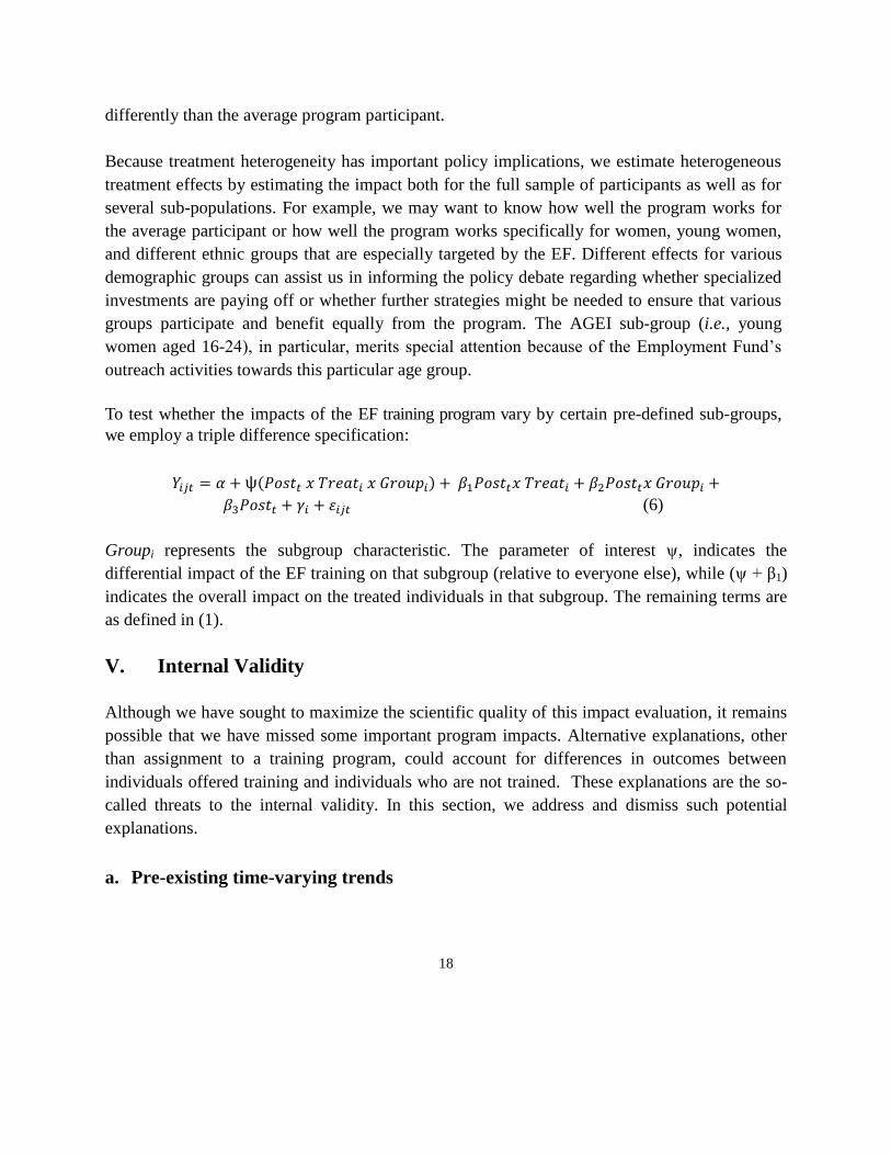
To test whether the impacts of the EF training program vary by certain pre-defined sub-groups,

we employ a triple difference specification:

( )

(6)

Groupi represents the subgroup characteristic. The parameter of interest ψ, indicates the

differential impact of the EF training on that subgroup (relative to everyone else), while (ψ + β1)

indicates the overall impact on the treated individuals in that subgroup. The remaining terms are

as defined in (1).

V. Internal Validity

Although we have sought to maximize the scientific quality of this impact evaluation, it remains

possible that we have missed some important program impacts. Alternative explanations, other

than assignment to a training program, could account for differences in outcomes between

individuals offered training and individuals who are not trained. These explanations are the so-

called threats to the internal validity. In this section, we address and dismiss such potential

explanations.

a. Pre-existing time-varying trends

19

We start by addressing concerns about pre-existing time-trends that could account for observed

training effects by comparing differences in characteristics between trainees and non-trainees.41

Towards that objective, we present “balancing tests” which capture the degree of similarity

between the two types of participants. Tables 4 and 5 present baseline participant characteristics

(i.e., balancing tests) for a set of 38 demographic indicators.42

These tests are based on “ITT”

comparisons of the treatment group (i.e., individuals whose scores qualify them for admission to

an EF training event) and the control group.

The baseline balance tests for 2010 (Table 4) and 2011 (Table 5) indicate that no significant

differences exist in the baseline observable characteristics of the treatment and control groups.43

This lends credibility to the evaluation methodology, which relies on the similarity between

treatment and control groups at baseline, although these results do not address concerns about

differences in unobservable characteristics or in time-varying characteristics. These baseline tests

have been repeated using an “ATT” comparison (in which the treatment group is defined based

on participation, rather than assignment to training). The ATT baseline tests also show no

significant differences in any of the variables. The baseline tests were also repeated after limiting

the sample to the area of common support and the results were extremely similar.

b. Survey response rates and attrition

One potential problem with any study such as ours is sample attrition. Approximately one year

after each baseline survey, we conducted a follow-up survey.44,45

The response rates were quite

high for both follow-up surveys (see Table 6). Overall, the survey firm was able to track and

successfully interview 89 percent of the baseline survey respondents.46

High response rates such

41 Characteristics of these two groups need not be the same for a difference-in-difference identification strategy to yield causal

effects; however, similar characteristics facilitate the empirical estimation. 42 Using a statistical tool called a student’s T test, we examine whether the difference in means between the two groups is

statistically significant. 43

The balance tests in Tables 4 and 5 use standard errors that are clustered by training event. We also ran the balance tests using

unclustered standard errors, and the results show significant differences in only 3 variables for 2010, and 4 variables in 2011. We

also conducted balance tests on a larger set of indicators, and again found very few differences. 44 Because the EF-sponsored training courses vary in length from 3 weeks to 3 months, the follow-up survey examines outcomes

9 to 11 months after the end of the training. 45 The EF itself conducts follow-up with a sample of participants up to 6 months after the training to verify employment and

earnings. Hence, the impact evaluation follow up survey occurs 3-5 months after the treatment group’s last contact with the

program. 46 The reasons given for loss to follow-up include: inability to track the household (11%), no one in the household during

multiple visits (15%), refusal (8%), respondent migrated for work within Nepal or abroad (8%), respondent migrated after

marriage (10%), or other (40%).

20

as these limit the degree to which any differences between respondents and non-respondents can

affect our estimates.

Particularly worrisome is the possibility of so-called “differential attrition”, a situation in which

we re-interview trainees and non-trainees at statistically different rates. Even with low attrition

rates for a panel survey, differential attrition may influence the scientific validity of results.

Suppose, hypothetically, that very motivated individuals in the control group (i.e., non-trainees)

are more likely, than trainees, to migrate to a district where they find employment. As a result of

this migration, these individuals will not show up in our analyses and this scenario could

compromise the scientific validity of this study’s estimates.

In Table 17, we explore this possibility and show no evidence to support it. Table 17 shows a

series of regressions on the correlates of survey attrition. For each cohort, we regress the panel

status of respondents on their treatment status, depending on how the treatment indicator is

defined. This specification provides information on whether treatment or control individuals are

more likely to be lost to follow-up. Next, we add a series of covariates, such as gender, age,

marital status, parental status, ethnicity, and employment, a set of district and T&E provider-

specific control dummy variables. The results indicate that differential attrition between

treatment and control groups is not an issue in this evaluation.

c. Uptake of EF-sponsored training courses

Another threat to our study is imperfect compliance, which occurs when those offered treatment

choose not to participate, or when people from the control group gain access to the program.

These deviations from treatment assignment may bias our estimates of program impact, because

the factors that determine one’s actual participation, such as motivation and tenacity, cannot be

observed and are likely correlated with the outcomes of interest.

Using administrative data from EF, we examine the rate of program take-up by the treatment and

control groups for the 2010 and 2011 cohorts in Table 7.47

The table shows a high degree of

uptake (65 to 74 percent) among the treatment group, but also a high rate of participation among

47 An individual is recorded in the EF monitoring database as a trainee only when the T&E provider submits the person’s name at

the end of the training. Since the EF only reimburses T&E providers at the conclusion of the training, they do not record nor do

we have any way to track how many people enrolled, but did not complete, the training.

21

the control group.48

Between 25 percent and 36 percent of the individuals in the control group

participated in the EF training course that they applied for, even though their scores did not

qualify them for admission. 49,50

In the presence of imperfect compliance, standard impact evaluation methods produce intent-to-

treat (ITT) estimates, as described in section IV. However, the relatively high degree of

noncompliance in our study leads to a likely downward bias in our ITT estimates, which

compare a treatment group in which not everyone received treatment to a control group in which

some people did receive treatment, hence diluting the impact of the program. We present an

alternative set of ATT estimates in Annex 3 in which we compare those who actually complete

training to those who do not, irrespective of treatment assignment.51

In our view, the ITT results

serve as a lower bound for the estimated program impact while the ATT results serve as an upper

bound.

VI. Short-Run Results of the EF Program

This section describes the impact of the Employment Fund’s training programs in 2010 and

2011. We measure outcomes approximately one year after the start of training.52

We start with a

description of our analysis on likelihood of being in the treatment group. We proceed with the

short-term impacts of the EF program on the full sample and on various demographic and socio-

economic sub-groups.

a. First-stage Estimation of Propensity Scores

48 The monitoring records indicate that the control group individuals who received training did so in the original training course

that they applied for. There is no evidence that they applied for and participated in a different EF training course sponsored by a

different T&E provider. 49 In practice, while we cannot be sure what happened in each case, the T&E providers probably dipped into the pool of lower-

scoring applicants in an attempt to fill up the training slots as people dropped out. 50 The stable unit treatment value assumption (i.e., SUTVA) based on Rubin (1980) assumes that (1) the treatment status of any

unit does not affect the potential outcomes of the other units (i.e., non-interference) and (2) the treatments for all units are

comparable (i.e., no variation in treatment). Note that take-up of training among control group units is not a violation of the

SUTVA, as take-up among non-beneficiaries was not directly a result of the take-up of training among the individuals selected

for training. 51 The ATT estimates suffer from an additional source of bias, since it is likely the “best” members of the control group who

gained access to the program and are reassigned to treatment in the ATT analysis, and the least motivated among those assigned

to treatment who fail to participate and are reassigned to control. See the discussion in Annex 3. 52 Because the EF-sponsored training courses vary in length from 3 weeks to 3 months, the follow-up survey examines outcomes

9 to 11 months after the end of the training.

22

At the heart of the propensity score matching method is pairing trainees with non-trainees who

are similar in terms of their observable characteristics. When the relevant differences between

any two units (i.e., trainees and non-trainees) are captured in the observable (pre-treatment)

covariates, the matching method can yield scientifically valid estimates of the impacts of

training. This pairing between a trainee and a comparable non-trainee is done via a propensity

score, as described in section IV.

Results from the propensity score estimation (shown in Table 8) exhibit only a few variables

correlated with an individual being offered training (i.e., treatment status). 53

This finding

reflects the high degree of similarity among short-listed candidates. The only characteristics

consistently correlated with an individual being assigned to a training program is being Muslim

or being a member of the Dalit ethnic group. Being married marginally lowers the likelihood of

gaining entry. No other variables are consistently correlated with training assignment, meaning

that within the pool of shortlisted candidates, there are few observable differences between those

selected for training and those who are not.

Based on a propensity score, we match each treated individual (i.e., a person assigned to a

training program) to one or more control observations (i.e., an individual or individuals who are

non-trainees) whose scores are equal or are near to the propensity score of the treatment

individual.54

We re-estimate the baseline balance tests and we drop individuals whose propensity scores lie

outside the area of common support.55,56

For each cohort and for each model, we find that the

variables showing statistically significant differences with the full sample remain statistically

significant. These results imply that the propensity score matching method does not substantially

improve the estimates obtained from the difference-in-difference method.

b. Impacts on Employment and Earnings for the Full Sample

53 We report the ITT results, for both the 2010 and 2011 cohorts. For the ITT first-stage probit, treatment is defined as having a

score that qualifies the respondent for admission to the EF training course to which s/he applied. 54 We remove any individuals whose scores are outside the range of common support. 55 It ensures that persons with the same X values have a positive probability of being both participants and non-participants

(Heckman, LaLonde, and Smith, 1999). Implementing the common support condition ensures that any combination of

characteristics observed in the treatment group can also be observed among the control group (Bryson, Dorsett, and Purdon,

2002) 56 The revised baseline balance tests, not shown, are almost identical to the original full-sample balance tests.

23

We estimate the program impact of the EF program using a combined propensity score matching

(PSM) and a difference-in-difference method. We use the three propensity score matching

(PSM) models: (1) Ordinary Least Squares (OLS), (2) Inverse Propensity Score Weighting (IPS),

and (3) Nearest-Neighbor matching (NN). The OLS and NN models use observations within the

area of common support only, while the IPS model uses the entire sample. In the OLS and IPS

models, we cluster the standard errors at the level of training courses.

Table 9 shows the ITT results on employment and earnings for the 2010 and 2011 cohorts.57

For

the 2010 cohort, we do not find (results in the first row of Table 9) evidence of consistent impact

on the employment rate.58

Only the IPS model indicates a positive and significant effect. This

finding is not surprising given the high employment rate (i.e., 60 percent) at baseline. However,

restricting the employment to non-farm activities, we find a significant increase for the 2010

cohort: the rate of participation in non-farm income-generating activities increases by 16 to 17

percentage points (from a base of 36.2 percent) for the ITT comparison. Translating the results in

percentage change terms, we find that the program increased non-farm employments by 44 to 47

percent. These impacts are not only statistically significant but also economically meaningful.

We also examine the trade-specific income generating activity (IGA) rate – the percent of

individuals who find employment in the same trade as the training that they applied for – and we

find impacts ranging from 19 to 20 percentage points. The trade-specific IGA impacts are larger

than the non-farm employment impacts, meaning that members of the control group, even when

able to find employment, were less able than the treatment group to find employment in the trade

in which they sought training.

Our results are considerably lower than estimates obtained by a simple before-and-after

comparison within the group of trainees. For the 2010 cohort, for example, the treatment group

had a non-farm employment rate of 37 percent at baseline and 68 percent at midline. A simple

difference in employment rates would have suggested that the program increased employment

rate by 31 percentage points (or 83 percent). However, comparison with the control group

reveals that non-farm employment improved over the same period for non-trainees also: the 2010

control group experiences non-farm employment increase by 15 percentage points. When we

examine the difference in differences59

, we detect program impact of 16 percentage points (or 45

percent).

57 We present results for the two cohorts separately due to differences in how events were sampled in 2010 and 2011. 58 We measure employment by whether the respondent reported any income-generating activities in the past month or not. 59 The change in the treatment group (31 percentage points) minus the change in the control group (15 percentage points)

24

The EF program also leads to persistent improvements in the underemployment rate (i.e., this

rate captures situations in which people are working fewer hours than they wish.) Table 9 shows

that EF-sponsored training courses increased hours worked in IGAs for the 2010 cohort by 21-28

hours per month (i.e., 26-38 percent). All three model specifications exhibit a statistically

significant and positive impact.

We detect strong program impacts on monthly earnings. We measure earnings as an individual’s

total earnings in the past month, including income from all IGAs, but not including unearned

income.60

We observe a statistically significant (at the 1 percent level) increase in monthly

earnings for the treatment group by 650 to 680 NRs (≈ 9 USD), from a baseline average of 1428

NRs (≈ 20 USD).61

In percentage terms, this earnings increase translates to a 45 percent for the

2010 cohort.

With alternative measurements of earnings, we detect even larger program impacts. To account

for the highly skewed nature of earnings distributions, we examine the impact on logged

earnings and we find impacts of over 100 percent. A third way to examine the impact on

earnings is to consider the proportion of participants who earned a “decent living.” The

Employment Fund considers 3000 NRs per month (≈ 40 USD) as “gainful employment” and

considers this amount as “being productively employed.” At baseline, only about 20 percent of

the sample was “gainfully employed”. The EF training program increased the “gainful

employment” rate increases by 12 to 14 percentage points, a result statistically significant across

all three models.

Program impacts for the 2011 cohort generally exhibit the same pattern (also in Table 9). Across

employment outcomes (first four rows of Table 9), the ITT results for the 2011 cohort are lower

than the ones for the 2010 cohort. The impact on non-farm employment ranges from 12 to 14

percentage points, compared to 15 to 17 percentage points for the 2010 cohort. The trade-specific

employment rate (i.e., the likelihood of obtaining employment in the same trade of one’s

training) ranges from 16 to 18 percentage points, compared to 19 to 20 percentage points for the

2010 cohort.

60 If an individual did not work in the past month, his/her earnings are recorded as zero. 61 This average is based on the entire study cohort, including those with zero earnings at baseline. The average earnings among

those with non-zero earnings were 2928 NRs, translating to a percentage increase in earnings of 22%.

25

Average program impacts on any measure of earnings for the 2011 cohort are uniformly higher

than for the 2010 cohort. For example, the training program impact on earnings increase for the

2010 cohort is 650 NRs (for the OLS results) as compared to the 764 NRs for the 2011 cohort, an

increase of 67 to 82 percent over the baseline average of 1130 NRs.62

The 2011 cohort data allows us to examine the impacts on rates of self-employment or work

outside of home. However, we find no evidence of persistent impact on either the rate of self-

employment or work outside of home.

c. Non-Employment Impacts for the Full Sample

Table 9’s last four rows present the estimated impacts on savings and borrowing behavior. We

find no systematic impacts of the EF training program on savings or loans for the 2010 cohort.

The final four rows of Table 9 also present the impacts on savings and borrowing for the 2011

cohort. The program had a significant and positive impact on individual savings – a year into the

program, savings increased by 926 to 1077 NRs (≈ 12 to 14 USD). No comparable treatment

effects on loan-taking for the 2011 cohort were detected.

Table 10 presents program impacts on a range of empowerment outcomes. Because

empowerment is a multi-dimensional concept, we examine various aspects of empowerment –

from psychological empowerment,63

entrepreneurial self-confidence,64

and financial literacy65

to

control over resources.66

The results show a very limited impact of the EF training program

across almost all of the empowerment measures for the 2010 and 2011 cohorts. The only

62 The baseline average earnings among those with non-zero earnings were 2723 NRs. 63 Psychological constructs related to self-confidence and self-regulation were measured using a series of questions to which the

respondent indicates their level of agreement (using variations of a Likert scale), which were then aggregated into a single score.

The self-regulation scale included questions on goal-setting and self-control. Preliminary reliability testing yielded a Cronbach’s

alpha of 0.77 for the self-regulation scale. 64 The entrepreneurial score is based on the respondent’s self- confidence to perform a series to tasks related to running a

business or searching for a job. The specific tasks asked were: Find information about job opportunities in your community,

Apply and interview for a job, Run your own business, Work in a team with 3-4 other people to accomplish a task, Identify

income generating activities to start up a new business, Obtain credit from a bank, microfinance institution, CBO or NGO,

Manage financial accounts, and Collect the money someone owes you. Respondents rated their ability to do these tasks on a scale

of 1 to 5, and their responses were summed to form a single numerical score. 65 Financial literacy is defined as responding correctly to at least one out of three questions indicating the respondent’s familiarity

with interest rates and ability to perform a mathematical computation (about one-third of respondents got the question right at

baseline) 66 Control over monetary resources is asked in a variety of ways in different sections of the survey questionnaire, including a

direct question on whether the respondent has any money of his own that he alone can decide how to use, whether he/she can

decide how to spend any earnings from employment or whether he/she needs permission, and whether he/she controls her own

savings, and the extent to which he/she participates in decisions regarding common household expenditures such as food and

medicine.

26

indicator that shows improvement is the self-regulation score for the 2011 cohort. The score

reflects the respondent’s self-reported ability to control impulses, delay gratification, stick to

difficult or detail-oriented tasks, and exert control over what happens in their life. The ITT

results for 2011 indicate a small but statistically significant increase of about 0.2 standard

deviations for the treatment group relative to control. There is no impact of a decline in

empowerment for any indicator.

A number of factors may explain the lack of impact observed in Table 10. Empowerment may

take longer to develop than just the one year between baseline and follow-up that this study

allows. Alternatively (or in addition), individuals’ sense of empowerment might increase but be

constrained by prevailing social and cultural norms. Or there may be changes in empowerment to

specific subgroups of respondents (e.g., women) but not the overall study population; this

possibility is explored in Section VIe. Finally, the indicators of empowerment employed in this

study might be not well-suited to the Nepali youth in this study. These factors, or a combination

of them, may explain the lack of impact on empowerment outcomes.

The final set of outcomes examined relate to reproductive health and household-level

outcomes.67

Table 11 shows that the EF program had no detectable effects on desired fertility for

either cohort. The program had mixed impacts on pregnancy, with a marginally significant

increase in 2010 and a marginally significant decline for the 2011 cohort. We find an increase in

marriage rates but that increase cannot account for the changes in pregnancies. A possible reason

difference in results could be partially due to the introduction of the life skills training for women

in 2011, which includes reproductive health topics, and is consistent with an increased use of

contraception among the treatment group in the 2011 cohort. However if the life skills training

were solely responsible for these changes in pregnancy and contraception use, the effects would

be expected to show up in the ATT results as well (see Annex 3). The EF training had no

detectable impact on HIV knowledge, on household food insecurity,68

or on protein

consumption.69

Although data for the 2011 cohort includes two additional indicators on

remittances, the program has no statistical effects on the receipt or amount of remittances

received.

67 The rationale for studying the effects of a job training program on reproductive health outcomes comes from the strong links

between employment and fertility decisions, particularly for female youth. When first entering the labor market, many youth are

making concurrent decisions about whether to pursue paid work outside the home, whether and when to start a family, and how

to balance the two. Previous impact evaluations have shown that empowerment in one realm (such as employment) can affect

decisions in other areas of life. 68 Measured using 4 questions adapted from the standard FANTA scale, with a higher score representing more insecurity. 69 Measured as whether the household consumes meat, fish, or eggs 5 or more times per week.

27

d. Trade-wise Program Impacts on the Full Sample

The Employment Fund sponsors about 600 training courses annually -- from short four-week

courses on incense-stick rolling to three-month technical courses. The breadth of course

offerings attracts individuals of varied training and career needs.70

Our evaluation sample

includes a bit more than 10 percent of the courses on offer each year (shown in Tables 1 and 2).

Panel 1 of Table 12 shows the breakdown of courses by trade.

We grouped training courses into seven categories.71

The most common categories of training in

our sample are Electrical/Electronics/Computer (e.g., electric wiring, computer hardware

technician, and mobile phone repair), Construction/Mechanical/Automobile (e.g., arc welding,

brick molding, furniture making, motor bike service), and Tailoring/Garment/Textile (e.g.,

galaicha weaving, garment fabrication, hand embroidery, tailoring and dressmaking). Because

we sample approximately the same number of applicants per event, the breakdown of applicants

by trade (Panel 2 of Table 12) is very similar to the event-wise breakdown.

Table 13 shows that the impacts of the skills training program differed markedly by type of trade

for both the 2010 and 2011 cohorts. Training in electronics, beautician, and tailoring consistently

show strong ITT impacts on employment—graduates of these training programs are more likely

to have employment in general and are also more likely to be working in the trade in which they

were trained. Beautician training shows large impacts on both employment and earnings. We

detect no consistent earnings impacts for other trades.

We detect no significant impacts on employment or earnings outcomes for the remaining four

trades. Results for food and hospitality (e.g., cooking and wait service) show no significant ITT

impacts; results for construction show no significant impacts except for an ITT impact on

earning more than 3000 NRs per month.72

For the remaining two trades (i.e., poultry technician

and handicrafts), we detect some ITT impacts but they are not consistent across models.

70 The Employment Fund mandates that all graduates sit for a skills certification test overseen by the National Skills Testing

Board (NSTB) for any trade in which such a test exists. Most of the EF training courses offer “Level 1” certification; in a few

trades the EF’s training providers also offer more advanced, or “Level 2” courses. 71 NSTB categories dictated groupings. 72 Construction is a unique case in which some labor demand comes from the Middle East and other foreign countries; the fact

that the construction trainings do not increase employment and earnings, regardless of location of employment, may help to

explain why no impacts on remittances were observed in Table 15.

28

The patterns for the 2011 cohort are very similar to the results for the 2010 cohort. Electronics,

beautician training, and tailoring continue to stand out as the highest performance categories of

training. We find that the training in food/hospitality and handicraft even led to some negative

ITT impacts, indicating that the control group had better outcomes than the treatment group,

though no negative impacts are found in the ATT analysis presented in Annex 3.

Overall, the results in Tables 13 reveal substantial heterogeneity in employment outcomes across

the various types of training. The positive and significant impacts discussed in Section VIb are

driven almost entirely by three categories of trades: electronics, beautician training, and tailoring

trades show positive and significant impacts on employment and earnings across both cohorts.

We find no impacts for the food/hospitality and handicraft training for either cohort, while

poultry technician training is not effective in 2010 (no training was offered for the 2011 sample).

Construction-related trainings showed positive and significant impacts, but the effects are not

consistent across outcomes or cohorts.73

e. Gender-disaggregated Impacts

An important objective of this report is to examine program impacts for men and women, and in

particular for the “AGEI” population (i.e., young women aged 16-24). To that end, Table 14

disaggregates the results for men, women, and the AGEI population, and the full sample.74

Table 14 shows striking differences for program impacts by gender. Generally, the impacts on

women are higher than the impacts on men. For the ITT effects for men, the results are not even

statistically significant, suggesting that women in the EF training program likely drive the overall

program impact. The higher impacts for women persist across outcomes, suggesting that the EF

training program is more effective at getting women into any employment, as well as into

employment specifically in their chosen trade, and better at increasing their earnings above the

3000 NRs/month mark than it is for men. Both the 2010 and 2011 cohorts exhibit these

differences for men and women.75

73 The difference in impacts may be driven by the types of training falling under this category (the 2010 sample includes more

brick-molding courses while 2011 includes more furniture making), the characteristics of the trainees (brick-molding is female-

dominated), or may reflect differences in the demand for construction labor in those two years. With the exception of poultry

training, all of the training categories were offered in several districts throughout the country, so it is unlikely that local market

differences are driving the observed differences in results. 74 For simplicity, we present only the Inverse Propensity Score (IPS) regression model results. 75 It is important to note that other than non-farm employment, the estimated difference between the impacts on men and women

is not statistically significant (this difference is not shown in table); this means that the results show clear evidence of a positive

and significant impact on women, but we find no significant impact for men.

29

The impacts on the employment outcomes for the AGEI sample resemble the ones for older

women. We detect no statistically significant differences between younger and older women,

meaning that the EF program appears to work equally well for the young women trained under

the AGEI.

Several factors – non-cognitive skills including motivation and perseverance, life-skills training,

baseline human capital differences and distance from the labor market, and type of training –

could account for the differential in program impacts between men and women. First, T&E

providers suggested that female students attend classes more and are more diligent than male

students. We lack data on the attendance or completion rates of EF trainees; however, the rate of

non-compliance with treatment assignment is equal for men and women, suggesting that this

mechanism is unlikely to exert much influence on outcomes. Second, the Employment Fund

introduced life skills training for women in 2011 in all of its training courses.76

Because all

women received life-skills training, we cannot disentangle the influence of this factor, from other

factors, on outcomes. A third explanation relates to men starting with a higher level of skills. In

our sample, men do have much higher rates of employment than women, at baseline and follow-

up. For women, the gains made by the treatment group exceed those of the control group by a

much larger margin, which lends some credence to this potential mechanism. A fourth possible

explanation relates to the difference between the types of trades that men and women apply for.

Although the Employment Fund specifically tries to encourage female participation in non-

traditionally female trades, most of the training courses tend to be heavily gender-segregated. For

example, men tend to dominate electronics and construction courses, while the tailoring and

beautician trainings are comprised almost exclusively of females. As shown earlier, the tailoring

and beautician trainings exhibit the largest employment impacts.77

Table 15 shows limited impacts on empowerment outcomes by gender. For the 2010 cohort, we

detect statistically significant positive impacts only for men, with regard to control over savings

and entrepreneurial orientation. The difference between men and women for these two outcomes

is also statistically significant (not shown in table). We also detect statistically significant (only

76 The forty-hour curriculum covered topics such as negotiation skills, workers’ rights, sexual and reproductive health, and

dealing with discrimination. Female students overwhelmingly responded positively to the life skills training, often claiming that it

was one of their favorite parts of the course. The skills learned and the positive experience in this life skills training may

contribute to the increased employment impact for women, which is line with the advice from experts in vocational training from

around the world, who increasingly advocate for the inclusion of life skills in technical training programs 77 It is entirely possible, in addition to the gender-related explanation, that occupations for which one obtains skills in the tailoring

and beautician courses are more profitable (relative to other occupations) in the Nepali labor market.

30

at 10 percent level) improvements in mobility for men. We detect no statistically significant

effects for the 2010 women’s and AGEI samples. Turning to the 2011 cohort, although the

impact on men for control over savings is significantly larger than the impact on women, women

report larger gains in control over earnings than men (and the difference is significant). These

positive effects apply to the younger AGEI sample as well, although there is also some evidence

of a decline in control over savings for the AGEI sample. Taken together, we interpret these

findings as providing no consistent impact on empowerment for men or women in 2010 or 2011.

There is limited evidence of an increase in empowerment among women in the ATT results in

Annex 3, suggesting that the estimated ITT impacts may be too diluted by dropouts to show any

significant improvements.

The final set of results, in Table 16, examines the impacts on reproductive health and family-

level outcomes by gender. Table 16 shows statistically significant impact only on pregnancy.

The increase in pregnancy in the 2010 cohort is reversed in the 2011 cohort, for which we see a

significant decline in pregnancy. Both impacts are driven by the AGEI subgroup. Overall, we do

not detect consistent impacts on pregnancy or on fertility. The increase in contraception reported

in Table 11 is shown here to be driven by the men in the sample, with no rise in contraceptive

use among the AGEI subgroup. We detect a statistically significant reduction in the number of

women who report “ever arguing with their spouse or partner in the past 12 months.” The ITT

effect is particularly strong for the AGEI subgroup and is statistically significant for the OLS

DID model as well (not shown in table). We detect no evidence of impacts on household level

outcomes on food security and remittances.

VII. Summary and Implications

In this section, we summarize the impacts of the Employment Fund’s training program. The EF

program aims to increase employment among Nepal’s disadvantaged youth through skills

training and job placement support. It is one of the largest providers of Technical Education and

Vocational Training (TEVT) in Nepal, and it works with local non-governmental training

providers to offer courses of up to three months in a variety of trades, followed by six months of

employment placement support.

To understand the effects of the EF program, we compared the experience of EF program

trainees with the experience of comparable non-trainees, approximately one year after the

program. Our sample included both male and female trainees, with a particular focus on the

AGEI population (i.e., females aged 16-24).

31

Approximately one year after each baseline survey, we conducted a follow-up survey. The

response rates were quite high for both follow-up surveys. Overall, the survey firm was able to

track and successfully interview 89 percent of the baseline survey respondents. We detect a high

degree of training uptake (82 to 86 percent) among the group offered training, but also a high

degree of participation among the control group. Between 25 percent and 36 percent of the

individuals in the control group participated in the EF training course that they applied for, even

though their scores did not qualify them for admission.

Using a combination of difference-in-difference and propensity score matching methods, we find

positive and statistically significant effects on labor market outcomes for EF trainees on the

following outcomes:

employment rates;

finding employment related to the skill they learned;

earnings; and

the proportion of people earnings more than 3000 NRs per month.

Individuals selected for EF training programs experience an increase in non-farm employment of

16-17 percentage points for an overall gain of 47 percent. We detect an increase in average

monthly earnings of approximately 45 percent. The gains for individuals who actually complete

the training (not just those who are selected for training) are even larger.

In contrast to the findings on employment outcomes, we find limited evidence of impacts on

empowerment, reproductive health, or household level outcomes.

Alongside the sizable general impacts on employment outcomes, we find that training courses in

electronics, beautician services, and tailoring underpin most of the EF program’s impacts. These

three categories of training are much more effective in consistently increasing employment and

earnings than construction, poultry rearing, handicrafts, and food preparation and hospitality.

We also find larger impacts for women than for men. Women selected for training in 2010 and

2011 experience non-farm and trade-specific employment gains of 20 to 22 percentage points,

while the impact for men is not statistically different from zero. Women’s earnings increase by

877 to 1142 NRs (equivalent to 12 to 15 USD) per month, while we cannot detect a statistically

significant increase in men’s earnings.

32

The impacts for young women aged 16 to 24 are not significantly different from those for older

women aged 25 to 35. This finding highlights the suitability of TEVT programs for younger

women, although it may require specialized outreach strategies to recruit them. The larger

impacts for women overall are consistent with the findings of rigorous evaluations of several

training programs in Latin America, though uncovering the reasons for these differences requires

further research. For women in the 2011 cohort, we also see positive and significant impacts on a

range of empowerment indicators, including control over earnings, self-regulation, and

entrepreneurial orientation.

The EF training program impacts are among the largest for training programs that have been

evaluated around the world. We posit two factors as possible explanations of these large impacts.

First, the EF had time to become established and to develop systems prior to the launch of the

impact evaluation in 2010. Most impact evaluations are conducted during the pilot stage of

project implementation, and consequently they do not always measure program impacts at their

best. In this evaluation, the program was already operating at scale, and the service delivery

processes already road-tested, which surely contribute to the large impacts. Second, the EF

program is designed around employment outcomes. For instance, training providers must

complete market assessments as part of their proposals to ensure future employability in the

trades in which they propose to train individuals. Training providers are rewarded with outcome-

based payments that are higher if they can demonstrate that their graduates have found work, a

policy which fosters an incentive to not just train young people, but to find jobs for them. The

fact that many training providers return year after year to work with the EF despite this unusual

contracting arrangement speaks to the feasibility of this approach.

These unique program features, along with the results shown in this evaluation, provide valuable

guidance and evidence for researchers, practitioners, and policy makers interested in improving

employment opportunities for young people in Nepal and around the world.

33

VIII. REFERENCES

Adoho, Franck, Shubha Chakravarty, Dala T. Korkoyah Jr., Mattias Lundberg, and Afia

Tasneem. 2013. "The Impact of an Adolescent Girls Program: The EPAG Project in Liberia" ,

Working Paper.

Aedo, Cristián and Sergio Nuñez. 2004. "The Impact of Training Policies in Latin America and

the Caribbean: The Case of Programa Joven" , Inter-American Development Bank Working

Paper #R-483.

Anderson, M. L. 2008. "Multiple Inference and Gender Differences in the Effects of Early

Intervention: A Reevaluation of the Abecedarian, Perry Preschool, and Early Training Projects"

Journal of the American Statistical Association, 103(484).

Angelucci, Manuela and Orazio P. Attanasio. 2006. "Estimating ATT Effects with Non-

Experimental Data and Low Compliance." , No. 2368. IZA Discussion Papers.

Attanasio, Orasio, Adriana Kugler, and Costas Meghir. 2008. "Training Disadvantaged

Youth in Latin America: Evidence from a Randomized Trial". NBER Working Paper 13931.

Bandiera, Oriana, Niklas Buehren, Robin Burgess, Markus Goldstein, Selim Gulesci,

Imran Rasul, and Munshi Sulaiman. 2012. “Empowering Adolescent Girls: Evidence from a

Randomized Control Trial in Uganda”. World Bank Working Paper No. 75566.

Betcherman, Gordon, Martin Godfrey, Olga Susana Puerto, Friederike Rother, and

Antoneta Stavreska. 2007. "Global Inventory of Interventions to Support Young Workers:

Synthesis Report" World Bank, Global Inventory of Interventions to Support Young Workers:

Synthesis Report.

Bryson, A., R. Dorsett, and S. Purdon. 2002. "The use of Propensity Score Matching in the

Evaluation of Labour Market Policies" , Working Paper No. 4, Department for Work and

Pensions.

Campbell, Donald T. 1969. "Reforms as Experiments" American Psychologist, 24: 407–429.

34

Card, D., J. Kluve, and A. Weber. 2009. "Active Labour Market Policy Evaluations: A

Metaanalysis" , Austrian Center for Labour Economics and the Analysis of the Welfare State

Working Paper, (0902).

Card, David, Pablo Ibarrarán, Ferdinando Regalia, David Rosas, and Yuri Soares. 2007.

"The Labor Market Impacts of Youth Training in the Dominican Republic: Evidence from a

Randomized Evaluation." , NBER Working paper 12883.

Fella, G. and G. Gallipoli. 2007. "Education and Crime Over the Life Cycle" , Rimini Center

15-07.

Frese, Michael and Gisela Mohr. 1987. "Prolonged Unemployment and Depression in Older

Workers: A Longitudinal Study of Intervening Variables" Social science & medicine, 25(2): 173-

178.

Gertler, Paul J., Sebastian Martinez, Patrick Premand, Laura B. Rawlings, and

Vermeersch. Christel M.J. 2011. Impact Evaluation in Practice: World Bank.

Goldsmith, Arthur H., Jonathan R. Veum, and William Darity. 1997. "The Impact of

Psychological and Human Capital on Wages" Economic inquiry, 35(4): 815-829.

Groh, Matthew, Nandini Krishnan, David McKenzie, and Tara Vishwanath. 2012. "Soft

Skills or Hard Cash? The Impact of Training and Wage Subsidy Programs on Female Youth

Employment in Jordan.". World Bank Policy Research Working Paper Series.

Heckman, J., R. LaLonde, and Smith J. 1999. "The Economics and Econometrics of Active

Labor Market Programs." In Handbook of Labor Economics , ed. O. Ashenfelter and David

Card, 1865-2097. Vol. III. Elsevier, Amsterdam.

Hopenhayn, Martin. 2002. "Youth and Employment in Latin America and the

Caribbean: Problems, Prospects and Options" , ECLAC Working Paper.

International Labor Organization (ILO). Youth Employment Statistics in Nepal. 2014.

http://apyouthnet.ilo.org/stats/youth-employment-statistics-in-nepal/at_download/file1 (accessed

September/1).

International Labor Organization (ILO). Labour market transitions of young women and men

in Nepal. Work 4 Youth Publication Series No. 12. May 2014.

Kling, Jeffrey R. and Jeffrey B. Liebman. 2004. Experimental Analysis of Neighborhood

Effects on Youth: John F. Kennedy School of Government, Harvard University.

35

Kluve, Jochen. 2006. "The Effectiveness of European Active Labor Market Policy" , IZA

Discussion Paper No. 2018; RWI Discussion Paper No. 37.

Leuven, E. and B. Sianesi. 2003. "PSMATCH2: Stata Module to Perform Full Mahalanobis and

Propensity Score Matching, Common Support Graphing and Covariate Imbalance Testing" ,

4.0.6 17may2012.(http://ideas.repec.org/c/boc/bocode/s432001.html).

Linn, M. W., R. Sandifer, and S. Stein. 1985. "Effects of Unemployment on Mental and

Physical Health" American Journal of Public Health, 75(5): 502-506.

Macours, Karen. 2011. “Increasing inequality and civil conflict in Nepal”. Oxford Economic

Papers, 63 (1).

Meyer, Bruce D. 1995. "Natural and Quasi-Experiments in Economics" Journal of Business and

Economic Statistics, 13(2): 151–161.

Ñopo, Hugo, Jaime Saavedra-Chanduví, and Miguel Robles. 2007. "Occupational Training to

Reduce Gender Segregation: The Impacts of ProJoven" , Inter-American Development Bank

Working Paper #623.

O'Brien, Peter C. 1984. "Procedures for Comparing Samples with Multiple Endpoints"

Biometrics: 1079-1087.

Robalino, D., Friederike Rother, David Newhouse, and Mattias Lundberg. 2013. "Youth

Unemployment: A Development Agenda for the Next Decade" , World Bank Social Protection

and Labor Discussion Paper no.1308.

Rosenbaum, P., and D. Rubin (1983): “The Central Role of the Propensity Score in Observational Studies

for Causal Effects,” Biometrika, 70, 41–50.

Rubin DB. 1980. "Randomization Analysis of Experimental Data in the Fisher Randomization

Test." Journal of the American Statistical Association, 75: 591–593.

Smith, Jeffrey and Petra E. Todd. 2005. "Does Matching Overcome Lalonde’s Critique of

Nonexperimental Estimators" Journal of Econometrics(125): 305–353.

Todd, Petra E. 2013. "How to Improve Women’s Employability and Quality of Work in

Developing and Transition Economies"

http://www.womeneconroadmap.org/sites/default/files/Todd_Improve%20Women%20Employabi

lity%20and%20Quality%20of%20Work.pdf.

The Employment Fund in Nepal

Impact Evaluation Report

ANNEXES

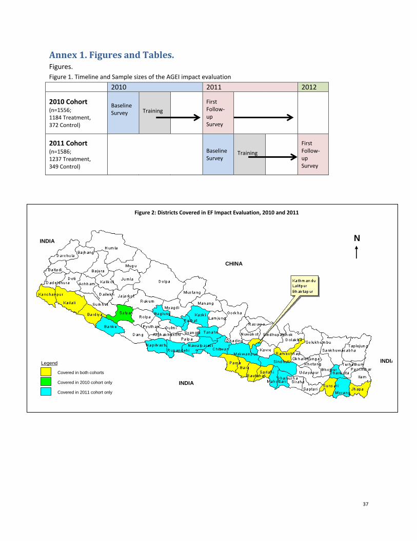
37

Annex 1. Figures and Tables. Figures.

Figure 1. Timeline and Sample sizes of the AGEI impact evaluation

2010 2011 2012

2010 Cohort (n=1556; 1184 Treatment, 372 Control)

Baseline Survey

Training

First Follow- up Survey

2011 Cohort (n=1586; 1237 Treatment, 349 Control)

Baseline Survey

Training

First Follow- up Survey

Figure 2: Districts Covered in EF Impact Evaluation, 2010 and 2011

N

INDIA Legend

Covered in 2011 cohort only

Covered in both cohorts

Covered in 2010 cohort only INDIA

CHINA

INDIA

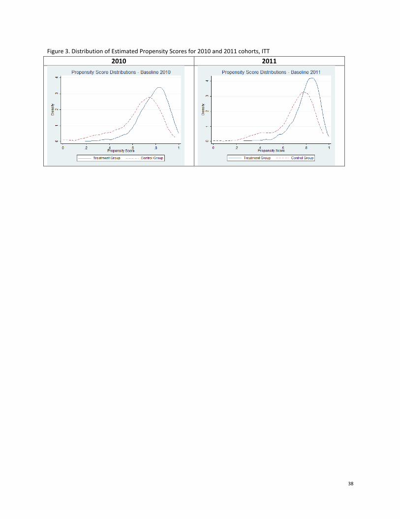
38

Figure 3. Distribution of Estimated Propensity Scores for 2010 and 2011 cohorts, ITT

2010 2011

39

Tables.

Table 1. Scale of Employment Fund Programs and AGEI Sub-group

All EF programs 2010 2011

Total T&E providers 21 32

Total Events 598 645

Total trained 11750 12869

AGEI only

T&E providers working with AGEI 11 13

Total Events 110 218

Total trained 808 1664

Table 2. Summary of Sample of Events for 2010 and 2011 Baseline Surveys

2010 2011

Total # events conducted by EF in Jan-Apr 110 142

# events randomly sampled N/A 182

# events included in baseline survey 65 69

# districts covered 30 34

# T&E providers covered 18 26 Note: more events were sampled than conducted in Jan-Apr 2011 because some events that were scheduled for Jan-Apr were delayed and did not start on time.

Table 3. Summary of Sample of Individuals for 2010 and 2011 Baseline Surveys

2010 2011 Pooled

Treatment group

Treatment- Male 478 447 925

Treatment- Female 706 790 1496

Treatment- all 1184 1237 2421

Control group

Control- Male 138 139 277

Control – Female 234 210 444

Control- all 372 349 721

Pooled (treatment and control)

Male 616 586 1202

Female 940 1000 1940

TOTAL 1556 1586 3142

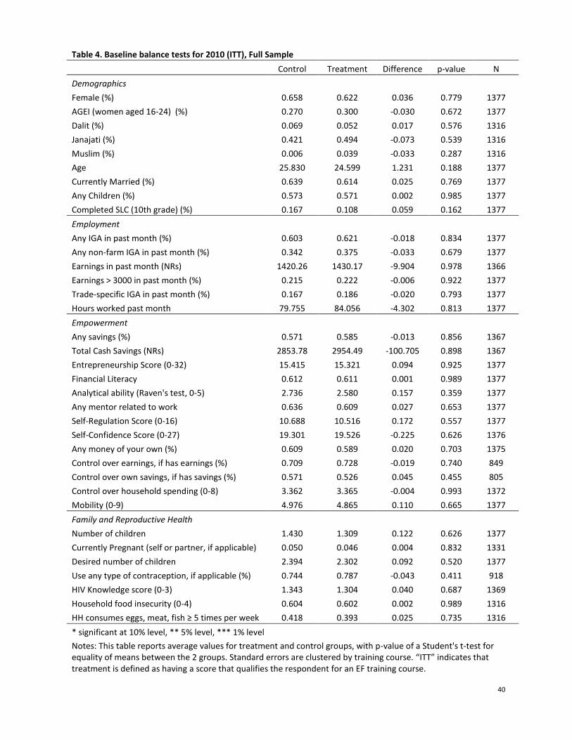
40

Table 4. Baseline balance tests for 2010 (ITT), Full Sample Control Treatment Difference p-value N

Demographics Female (%) 0.658 0.622 0.036 0.779 1377

AGEI (women aged 16-24) (%) 0.270 0.300 -0.030 0.672 1377

Dalit (%) 0.069 0.052 0.017 0.576 1316

Janajati (%) 0.421 0.494 -0.073 0.539 1316

Muslim (%) 0.006 0.039 -0.033 0.287 1316

Age 25.830 24.599 1.231 0.188 1377

Currently Married (%) 0.639 0.614 0.025 0.769 1377

Any Children (%) 0.573 0.571 0.002 0.985 1377

Completed SLC (10th grade) (%) 0.167 0.108 0.059 0.162 1377

Employment Any IGA in past month (%) 0.603 0.621 -0.018 0.834 1377

Any non-farm IGA in past month (%) 0.342 0.375 -0.033 0.679 1377

Earnings in past month (NRs) 1420.26 1430.17 -9.904 0.978 1366

Earnings > 3000 in past month (%) 0.215 0.222 -0.006 0.922 1377

Trade-specific IGA in past month (%) 0.167 0.186 -0.020 0.793 1377

Hours worked past month 79.755 84.056 -4.302 0.813 1377

Empowerment Any savings (%) 0.571 0.585 -0.013 0.856 1367

Total Cash Savings (NRs) 2853.78 2954.49 -100.705 0.898 1367

Entrepreneurship Score (0-32) 15.415 15.321 0.094 0.925 1377

Financial Literacy 0.612 0.611 0.001 0.989 1377

Analytical ability (Raven's test, 0-5) 2.736 2.580 0.157 0.359 1377

Any mentor related to work 0.636 0.609 0.027 0.653 1377

Self-Regulation Score (0-16) 10.688 10.516 0.172 0.557 1377

Self-Confidence Score (0-27) 19.301 19.526 -0.225 0.626 1376

Any money of your own (%) 0.609 0.589 0.020 0.703 1375

Control over earnings, if has earnings (%) 0.709 0.728 -0.019 0.740 849

Control over own savings, if has savings (%) 0.571 0.526 0.045 0.455 805

Control over household spending (0-8) 3.362 3.365 -0.004 0.993 1372

Mobility (0-9) 4.976 4.865 0.110 0.665 1377

Family and Reproductive Health Number of children 1.430 1.309 0.122 0.626 1377

Currently Pregnant (self or partner, if applicable) 0.050 0.046 0.004 0.832 1331

Desired number of children 2.394 2.302 0.092 0.520 1377

Use any type of contraception, if applicable (%) 0.744 0.787 -0.043 0.411 918

HIV Knowledge score (0-3) 1.343 1.304 0.040 0.687 1369

Household food insecurity (0-4) 0.604 0.602 0.002 0.989 1316

HH consumes eggs, meat, fish ≥ 5 times per week 0.418 0.393 0.025 0.735 1316

* significant at 10% level, ** 5% level, *** 1% level Notes: This table reports average values for treatment and control groups, with p-value of a Student's t-test for

equality of means between the 2 groups. Standard errors are clustered by training course. “ITT” indicates that treatment is defined as having a score that qualifies the respondent for an EF training course.

41

Table 5. Baseline balance tests for 2011 (ITT), Full Sample Control Treatment Difference p-value N

Demographics Female (%) 0.637 0.668 -0.031 0.806 1419

AGEI (women aged 16-24) (%) 0.399 0.408 -0.009 0.910 1419

Dalit (%) 0.101 0.111 -0.009 0.856 1419

Janajati (%) 0.359 0.429 -0.069 0.440 1419

Muslim (%) 0.023 0.030 -0.007 0.819 1419

Age 23.10 23.49 -0.392 0.517 1419

Currently Married (%) 0.526 0.545 -0.019 0.779 1419

Any Children (%) 0.425 0.473 -0.049 0.487 1419

Completed SLC (10th grade) (%) 0.134 0.103 0.031 0.478 1419

Any previous skills training (%) 0.212 0.167 0.045 0.380 1419

Employment Any IGA in past month (%) 0.552 0.597 -0.045 0.657 1419

Any non-farm IGA in past month (%) 0.222 0.289 -0.067 0.368 1419

Earnings in past month (NRs) 1004.27 1165.69 -161.419 0.602 1406

Earnings > 3000 in past month (%) 0.121 0.174 -0.053 0.302 1419

Trade-specific IGA in past month (%) 0.105 0.149 -0.045 0.511 1419

Hours worked past month 51.206 63.971 -12.765 0.368 1419

Self-employed (%) 0.330 0.317 0.013 0.862 1419

Empowerment Any savings (%) 0.561 0.631 -0.070 0.295 1401

Total Cash Savings (NRs) 2730.22 2807.23 -77.010 0.909 1401

Entrepreneurship Score (0-32) 14.572 14.579 -0.007 0.994 1419

Financial Literacy 0.598 0.581 0.017 0.782 1419

Analytical ability (Raven's test, 0-5) 3.036 3.051 -0.015 0.922 1419

Any mentor Related to work 0.572 0.581 -0.009 0.905 1417

Self-Regulation Score (0-16) 10.337 10.162 0.175 0.681 1419

Self-Confidence Score (0-27) 18.418 18.464 -0.045 0.913 1419

Any money of your own (%) 0.674 0.705 -0.031 0.523 1414

Control over earnings, if has earnings (%) 0.604 0.621 -0.018 0.818 834

Control over own savings, if has savings (%) 0.572 0.569 0.003 0.958 881

Control over household spending (0-8) 2.717 3.028 -0.311 0.489 1415

Mobility (0-9) 4.510 4.435 0.075 0.786 1419

Family and Reproductive Health Number of children 0.837 0.957 -0.120 0.509 1419

Currently Pregnant (self or partner, if applicable) 0.027 0.038 -0.011 0.449 1315

Desired number of children 2.098 2.120 -0.022 0.792 1419 Use any type of contraception, if applicable (%) 0.780 0.776 0.004 0.946 844 HIV Knowledge score (0-3) 1.152 1.104 0.048 0.651 1391

Household food insecurity (0-4) 0.551 0.540 0.011 0.910 1389 HH consumes eggs, meat, fish ≥ 5 times per week 0.328 0.369 -0.041 0.625 1262 Household receives remittances (%) 0.247 0.224 0.022 0.645 1389

* significant at 10% level, ** 5% level, *** 1% level

Notes: This table reports average values for treatment and control groups, with p-value of a Student's t-test for equality of means between the 2 groups. Standard errors are clustered by training course. “ITT” indicates that treatment is defined as having a score that qualifies the respondent for an EF training course.

42

Table 6. Survey response rates

Baseline Follow-up Follow-up

rate

2010 cohort

Treatment 1184 1047 88.43%

Control 372 330 88.71%

Total 1556 1377 88.50%

2011 cohort

Treatment 1237 1113 89.98%

Control 349 306 87.68%

Total 1586 1419 89.40%

Note: This table uses “ITT” treatment status- those whose scores qualify them for training.

Table 7. Uptake of EF-sponsored training in the year following baseline survey

Participated in an EF training course

Did not participate in an EF training course

Number Percent Number Percent

2010 Cohort (n=1372*)

Assigned to Treatment (n=1040) 671 64.52%

369 35.48%

Assigned to Control (n=332) 86 25.90%

246 74.10%

2011 Cohort (n=1415*)

Assigned to Treatment (n=1110) 826 74.41%

284 25.59%

Assigned to Control (n=305) 110 36.07% 195 63.93%

* note: there are 4 people from the 2011 cohort and 5 people from 2010 whose status in the EF database is unknown. For these individuals, we rely on the respondent’s self-report of whether they took an EF training in the past year for the ATT results.

Note: The table only includes those individuals who were surveyed for the first follow-up.

43

Table 8. First-stage Estimation of Propensity Scores

Dependent variable: Treat (ITT)

(1) (2)

Age of applicant 0.010 0.011

(0.017) (0.021)

Sex of applicant (1=Female) -0.313* 0.101

(0.164) (0.216)

Education level of applicant -0.023 0.004

(0.017) (0.019)

Education of hh head -0.028*** 0.013

(0.010) (0.013)

Household size -0.003 0.003

(0.012) (0.011)

Married (1=Yes) -0.318** -0.218*

(0.128) (0.118)

Has child (1=Yes) 0.445** 0.195

(0.189) (0.165)

Number of children -0.085 -0.056

(0.069) (0.080)

Any IGA (1= Yes) 0.123 0.153

(0.162) (0.141)

Zero earnings (1=Yes) 0.093 -0.180

(0.158) (0.129)

Janajati (1=Yes) -0.162 0.235

(0.563) (0.742)

Dalit (1=Yes) 4.868*** 5.110***

(0.540) (0.670)

Muslim (1=Yes) 4.839*** 4.426***

(0.455) (0.631)

Analytical Ability (0-5) -0.070** 0.008

(0.030) (0.042)

Entrepreneurial score (0-32) 0.013 0.002

(0.008) (0.008)

Financial literacy (1=Yes) 0.077 -0.166*

(0.109) (0.101)

Any previous skills training -0.216*

(0.112)

N 1378 1506

Cohort 2010 2011

Notes: * Significant at 10% level ** 5% *** 1% Standard errors (reported in brackets) clustered by training course. "Treat (ITT)" equals 1 if individual qualified for a training course. Other independent variables (not shown): district and T&E provider fixed effects, training-type categories, quintiles of hh wealth. All variables measured at baseline. Note that questions about previous skills trainings were not asked in 2010.

44

Table 9. Employment outcomes (ITT), 2010 + 2011 cohort 2010 Cohort 2011 Cohort

Baseline mean OLS IPS NN Baseline mean OLS IPS NN

[Std Dev] (1) (2) (3)

[Std Dev] (4) (5) (6)

Any IGA (1=Yes) 0.617 0.040 0.086* 0.037

0.588 0.062 0.103** 0.053

[0.486] (0.034) (0.044) (0.035)

[0.492] (0.042) (0.046) (0.037)

Any non-farm IGA (1=Yes) 0.367 0.157*** 0.167*** 0.158***

0.275 0.125*** 0.139*** 0.117***

[0.482] (0.045) (0.046) (0.038)

[0.447] (0.041) (0.046) (0.037)

Trade-specific IGA (1=Yes) 0.182 0.197*** 0.185*** 0.201***

0.140 0.162*** 0.180*** 0.163***

[0.386] (0.046) (0.052) (0.036)

[0.347] (0.043) (0.046) (0.035)

Hours worked in past month 83.025 21.254*** 28.007*** 21.201***

61.218 18.957*** 26.052*** 18.208***

[97.602] (6.393) (7.394) (7.446)

[82.633] (7.017) (8.023) (6.604)

Earnings 1427.796 649.371** 669.082** 681.026***

1130.906 763.930*** 930.448*** 774.953***

[2181.198] (269.218) (263.132) (213.852)

[2067.13] (207.048) (245.458) (200.504)

Logged earnings 3.715 1.008*** 0.927** 1.004***

3.111 1.026*** 1.594*** 0.965***

[3.87] (0.345) (0.349) (0.312)

[3.748] (0.339) (0.419) (0.309)

Earnings > 3000 NRs. (1=Yes) 0.220 0.124*** 0.144*** 0.125***

0.163 0.132*** 0.147*** 0.133***

[0.414] (0.039) (0.040) (0.037)

[0.369] (0.040) (0.043) (0.037)

Self-Employed (1=Yes), if any IGA

0.320 0.030 0.038 0.029

[0.467] (0.050) (0.051) (0.041)

Works outside of home (1=Yes)

0.627 0.041 0.044 0.038

[0.484] (0.054) (0.063) (0.056)

Any Savings (1=Yes) 0.582 0.022 0.022 0.025

0.616 0.026 0.039 0.031

[0.493] (0.038) (0.042) (0.037)

[0.487] (0.047) (0.051) (0.039)

Total Savings (NRs). 2930.252 357.287 745.915 288.980

2790.570 935.067** 926.316* 1076.830*

[6955.561] (645.068) (727.215) (636.021)

[6442.042] (404.779) (477.172) (566.943)

Logged Savings 4.386 0.206 0.320 0.221

4.546 0.467 0.503 0.486

[3.891] (0.278) (0.341) (0.287)

[3.781] (0.334) (0.383) (0.298)

Taken out loan (1=Yes) 0.373 0.005 0.017 0.011

0.312 -0.019 -0.003 -0.018

[0.484] (0.037) (0.045) (0.035)

[0.464] (0.037) (0.046) (0.033) Clustered Standard Errors Yes Yes No Yes Yes No

Notes: All columns report difference-in-difference estimates. "ITT" indicates that everyone whose score qualified them for a given training event is included in the "treatment" group. Standard errors (reported in brackets) clustered at the event level where possible. Self-employment and location of work were not asked in 2010. * Significant at 10% level ** 5% *** 1%

45

Table 10. Empowerment outcomes (ITT), 2010+2011 cohort 2010 Cohort 2011 Cohort

Baseline mean OLS IPS NN Baseline mean OLS IPS NN

[Std Dev] (1) (2) (3)

[Std Dev] (1) (2) (3)

Any money of your own (1=Yes)

0.594 -0.005 0.004 0.003

0.699 0.011 -0.009 0.007

[0.491] (0.037) (0.040) (0.038)

[0.459] (0.045) (0.046) (0.037)

Control over Earnings (1=Yes), if respondent has earnings

0.723 -0.008 -0.039 -0.008

0.618 0.077 0.072 0.069

[0.448] (0.049) (0.058) (0.051)

[0.486] (0.058) (0.060) (0.055)

Control Over Savings (1=Yes), if respondent has savings

0.537 0.052 0.095 0.053

0.57 -0.039 -0.037 -0.051

[0.499] (0.053) (0.057) (0.059)

[0.495] (0.055) (0.067) (0.064)

Control over household spending (# categories out of 8)

3.364 0.175 0.484* 0.202

2.961 0.089 -0.108 0.010

[3.191] (0.206) (0.276) (0.214)

[3.217] (0.185) (0.229) (0.204)

Mobility (# places visited in last month out of 9)

4.892 0.161 0.171 0.131

4.451 0.098 0.033 0.084

[1.735] (0.149) (0.148) (0.133)

[1.709] (0.132) (0.149) (0.136)

Any Mentor Related to Work (1=Yes)

0.616 0.062 0.036 0.061

0.579 0.059 0.048 0.056

[0.487] (0.044) (0.042) (0.039)

[0.494] (0.039) (0.049) (0.041)

Entrepreneurship Score (0-32) 15.344 0.188 0.809 0.140

14.577 0.113 -0.036 0.062

[6.408] (0.505) (0.554) (0.503)

[5.665] (0.477) (0.510) (0.472)

Financial Literacy (1=Yes) 0.611 -0.015 0.003 -0.019

0.585 0.001 0.029 -0.000

[0.488] (0.049) (0.052) (0.043)

[0.493] (0.047) (0.053) (0.042)

Self-Regulation Score (0-16) 10.557 0.234 0.279 0.275

10.199 0.494** 0.471* 0.476**

[2.294] (0.231) (0.242) (0.209)

[2.483] (0.209) (0.252) (0.195)

Self-Confidence Score (0-27) 19.472 -0.019 -0.023 -0.089

18.454 0.269 0.119 0.237

[3.632] (0.330) (0.304) (0.310)

[3.099] (0.258) (0.301) (0.272)

Clustered Standard Errors Yes Yes No Yes Yes No Notes: All columns report difference-in-difference estimates. "ITT" indicates that everyone whose score qualified them for a given training event is included in the "treatment"

group. Standard errors (reported in brackets) clustered at the event level where possible.

* Significant at 10% level ** 5% *** 1%

46

Table 11. Family and reproductive health outcomes (ITT), 2010 + 2011 cohort 2010 Cohort

2011 Cohort

Baseline mean OLS IPS NN

Baseline mean OLS IPS NN

[Std Dev] (1) (2) (3)

[Std Dev] (1) (2) (3)

Desired number of children 2.324 0.041 0.028 0.038

2.116 -0.022 -0.038 -0.024

0.898 (0.043) (0.055) (0.035)

[0.649] (0.040) (0.045) (0.036)

Pregnant (1= Yes), if married 0.047 0.036* 0.051** 0.036* 0.036 -0.036* -0.042* -0.035*

[0.212] (0.019) (0.024) (0.020) [0.186] (0.019) (0.023) (0.019)

Number of children, if respondent has children

1.338 -0.052 -0.059* -0.050 0.931 0.011 0.023 0.010

[1.454] (0.038) (0.035) (0.035) [1.204] (0.020) (0.018) (0.018)

Ever argue with spouse/ partner, if applicable (1=Yes)

0.841 -0.060 -0.037 -0.072*

0.778 -0.031 -0.012 -0.031

[0.366] (0.040) (0.035) (0.038)

[0.416] (0.043) (0.041) (0.045)

Use any type of contraception (1=Yes), if sexually active

0.777 -0.044 -0.051 -0.045

0.777 0.093** 0.111*** 0.079*

[0.417] (0.038) (0.039) (0.038)

[0.416] (0.038) (0.040) (0.042)

HIV Knowledge score (0-3) 1.313 -0.096 -0.050 -0.084

1.114 0.073 0.084 0.067

[0.687] (0.072) (0.083) (0.073)

[0.788] (0.073) (0.075) (0.066)

Household food insecurity (0-4)

0.603 0.015 -0.017 0.015

0.542 0.016 -0.043 0.019

[0.829] (0.054) (0.060) (0.057)

[0.781] (0.056) (0.070) (0.058)

Household receives remittances (1=Yes)

0.399 -- -- --

0.361 -0.027 -0.018 -0.027

[0.490]

[0.480] (0.037) (0.043) (0.030)

Household received more remittances than last year (1=Yes)

-- -- --

0.229 0.003 -0.001 0.012

[0.42] (0.027) (0.027) (0.026)

Clustered Standard Errors Yes Yes No Yes Yes No Notes: All columns report difference-in-difference estimates. "ITT" indicates that everyone whose score qualified them for a given training event is included in the "treatment"

group. Standard errors (reported in brackets) clustered at the event level where possible. Remittance questions were not asked in 2010.

* Significant at 10% level ** 5% *** 1%

47

Table 12. Tabulation of training types Panel 1: Event-wise tabulation 2010 2011

Number % Number %

Poultry 2 3 0 0

Food Prep/ Hospitality 11 17 3 4

Electrical/ Electronics/Computer 9 14 14 20

Handicraft & Incense 3 4 4 6

Construction/Mechanical/Automobile 20 31 13 19

Beautician /Barber 2 3 5 7

Tailoring/ Garment/Textile 18 28 30 44

TOTAL 65 100 69 100

Panel 2: Applicant-wise tabulation 2010 2011

Number % Number %

Poultry 41 3 0 0

Food Prep/ Hospitality 195 14 38 3

Electrical/ Electronics/Computer 178 13 277 19

Handicraft & Incense 87 6 79 6

Construction/Mechanical/Automobile 413 30 258 18

Beautician /Barber 61 4 117 8

Tailoring/ Garment/Textile 415 30 650 46

TOTAL 1390 100 1419 100

Note: this table only includes panel observations (those who were interviewed at baseline and midline).

48

Table 13. Employment outcomes disaggregated by trade

2010 Cohort IPS Model ITT Effects

2011 Cohort IPS Model ITT Effects

any nonfarm

IGA

trade-specific

IGA

monthly earnings

(NRs) earnings >

3000

any nonfarm

IGA

trade-specific

IGA

monthly earnings

(NRs) earnings >

3000

(1) (2) (3) (4) (5) (6) (7) (8)

Full Sample (pooled across training types) 0.167*** 0.185*** 669.082** 0.144***

0.139*** 0.180*** 930.448*** 0.147***

(0.046) (0.052) (263.132) (0.040)

(0.046) (0.046) (245.458) (0.043)

training: Poultry Technician 0.335* 0.373*** 588.918 0.134

N/A N/A N/A N/A

n=41 (2010), 0 (2011) (0.180) (0.141) (1253.294) (0.160) training: Food prep/Hospitality 0.009 -0.058 -711.341 -0.057

-0.712** -0.161 -4814.601* -1.007***

n=195 (2010), 38 (2011) (0.085) (0.083) (493.529) (0.045)

(0.311) (0.161) (2490.210) (0.284)

training: Electrician & Electronics 0.230** 0.393*** 1437.729 0.228

0.100 0.215** 782.756* 0.128*

n=178 (2010), 277 (2011) (0.108) (0.109) (953.444) (0.143)

(0.063) (0.109) (410.322) (0.073)

training: Handicraft & Incense stick making 0.219*** 0.159 960.538* 0.143

-0.226*** -0.130 -492.406 -0.027

n=87 (2010), 79 (2011) (0.068) (0.134) (570.089) (0.213)

(0.066) (0.080) (765.500) (0.067)

training: Construction 0.076 0.056 440.101 0.180***

0.077 0.145 723.690* 0.094

n=413 (2010), 258 (2011) (0.091) (0.114) (446.228) (0.056)

(0.115) (0.131) (427.482) (0.095)

training: Beautician/Barber 0.581*** 0.612*** 3249.29*** 0.470***

0.083 0.219** 1067.88*** 0.023

n=61 (2010), 117 (2011) (0.075) (0.099) (160.937) (0.030)

(0.099) (0.106) (224.687) (0.133)

training: Weaving/Tailoring/Garment Making 0.195** 0.245*** 629.438 0.103

0.262*** 0.223*** 1387.36*** 0.249***

n=415 (2010), 650 (2011) (0.085) (0.078) (433.392) (0.073)

(0.067) (0.062) (377.310) (0.060)

Clustered standard errors (by event) Yes Yes Yes Yes Yes Yes Yes Yes

Note: No poultry technician trainings were included in the 2011 sample.

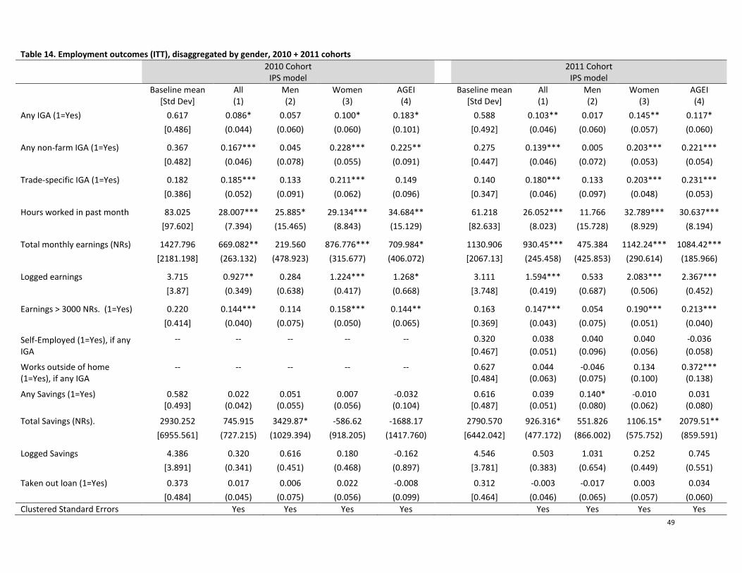
49

Table 14. Employment outcomes (ITT), disaggregated by gender, 2010 + 2011 cohorts

2010 Cohort

IPS model 2011 Cohort

IPS model

Baseline mean All Men Women AGEI Baseline mean All Men Women AGEI

[Std Dev] (1) (2) (3) (4)

[Std Dev] (1) (2) (3) (4)

Any IGA (1=Yes) 0.617 0.086* 0.057 0.100* 0.183*

0.588 0.103** 0.017 0.145** 0.117*

[0.486] (0.044) (0.060) (0.060) (0.101)

[0.492] (0.046) (0.060) (0.057) (0.060)

Any non-farm IGA (1=Yes) 0.367 0.167*** 0.045 0.228*** 0.225**

0.275 0.139*** 0.005 0.203*** 0.221***

[0.482] (0.046) (0.078) (0.055) (0.091)

[0.447] (0.046) (0.072) (0.053) (0.054)

Trade-specific IGA (1=Yes) 0.182 0.185*** 0.133 0.211*** 0.149

0.140 0.180*** 0.133 0.203*** 0.231***

[0.386] (0.052) (0.091) (0.062) (0.096)

[0.347] (0.046) (0.097) (0.048) (0.053)

Hours worked in past month 83.025 28.007*** 25.885* 29.134*** 34.684**

61.218 26.052*** 11.766 32.789*** 30.637***

[97.602] (7.394) (15.465) (8.843) (15.129)

[82.633] (8.023) (15.728) (8.929) (8.194)

Total monthly earnings (NRs) 1427.796 669.082** 219.560 876.776*** 709.984*

1130.906 930.45*** 475.384 1142.24*** 1084.42***

[2181.198] (263.132) (478.923) (315.677) (406.072)

[2067.13] (245.458) (425.853) (290.614) (185.966)

Logged earnings 3.715 0.927** 0.284 1.224*** 1.268*

3.111 1.594*** 0.533 2.083*** 2.367***

[3.87] (0.349) (0.638) (0.417) (0.668)

[3.748] (0.419) (0.687) (0.506) (0.452)

Earnings > 3000 NRs. (1=Yes) 0.220 0.144*** 0.114 0.158*** 0.144**

0.163 0.147*** 0.054 0.190*** 0.213***

[0.414] (0.040) (0.075) (0.050) (0.065)

[0.369] (0.043) (0.075) (0.051) (0.040)

Self-Employed (1=Yes), if any IGA

-- -- -- -- --

0.320 0.038 0.040 0.040 -0.036

[0.467] (0.051) (0.096) (0.056) (0.058)

Works outside of home (1=Yes), if any IGA

-- -- -- -- --

0.627 0.044 -0.046 0.134 0.372***

[0.484] (0.063) (0.075) (0.100) (0.138)

Any Savings (1=Yes) 0.582 0.022 0.051 0.007 -0.032

0.616 0.039 0.140* -0.010 0.031

[0.493] (0.042) (0.055) (0.056) (0.104)

[0.487] (0.051) (0.080) (0.062) (0.080)

Total Savings (NRs). 2930.252 745.915 3429.87* -586.62 -1688.17

2790.570 926.316* 551.826 1106.15* 2079.51**

[6955.561] (727.215) (1029.394) (918.205) (1417.760)

[6442.042] (477.172) (866.002) (575.752) (859.591)

Logged Savings 4.386 0.320 0.616 0.180 -0.162

4.546 0.503 1.031 0.252 0.745

[3.891] (0.341) (0.451) (0.468) (0.897)

[3.781] (0.383) (0.654) (0.449) (0.551)

Taken out loan (1=Yes) 0.373 0.017 0.006 0.022 -0.008

0.312 -0.003 -0.017 0.003 0.034

[0.484] (0.045) (0.075) (0.056) (0.099)

[0.464] (0.046) (0.065) (0.057) (0.060)

Clustered Standard Errors Yes Yes Yes Yes Yes Yes Yes Yes

50

Table 15. Empowerment outcomes (ITT), disaggregated by gender, 2010 + 2011 cohort

2010 Cohort

IPS model 2011 Cohort

IPS model

Baseline mean All Men Women AGEI Baseline mean All Men Women AGEI

[Std Dev] (1) (2) (3) (4)

[Std Dev] (1) (2) (3) (4)

Any money of your own (1=Yes)

0.594 0.004 0.106 -0.047 0.003

0.699 -0.009 -0.089 0.029 0.026

[0.491] (0.040) (0.068) (0.047) (0.068)

[0.459] (0.046) (0.054) (0.061) (0.074)

Control over Earnings (1=Yes), if respondent has earnings

0.723 -0.039 0.001 -0.074 -0.128

0.618 0.072 -0.078 0.220*** 0.346**

[0.448] (0.058) (0.069) (0.090) (0.137)

[0.486] (0.060) (0.087) (0.081) (0.148)

Control Over Savings (1=Yes), if respondent has savings

0.537 0.095 0.246*** 0.029 -0.046

0.57 -0.037 0.214** -0.109 -0.215**

[0.499] (0.057) (0.073) (0.066) (0.134)

[0.495] (0.067) (0.094) (0.080) (0.101)

Control over household spending (# categories)

3.364 0.484* 0.434 0.509 1.054

2.961 -0.108 0.321 -0.311 -0.090

[3.191] (0.276) (0.312) (0.392) (0.725)

[3.217] (0.229) (0.463) (0.250) (0.284)

Mobility (# places visited in last month out of 9)

4.892 0.171 0.464* 0.024 0.009

4.451 0.033 -0.055 0.079 0.154

[1.735] (0.148) (0.252) (0.178) (0.250)

[1.709] (0.149) (0.211) (0.191) (0.229)

Any Mentor Related to Work (1=Yes)

0.616 0.036 -0.038 0.073 0.046

0.579 0.048 -0.042 0.090 0.119

[0.487] (0.042) (0.066) (0.051) (0.082)

[0.494] (0.049) (0.077) (0.058) (0.085)

Entrepreneurship Score (0-32) 15.344 0.809 2.903*** -0.236 0.020

14.577 -0.036 0.106 -0.122 1.145*

[6.408] (0.554) (0.808) (0.701) (1.224)

[5.665] (0.510) (0.753) (0.686) (0.677)

Financial Literacy (1=Yes) 0.611 0.003 -0.012 0.012 -0.113

0.585 0.029 -0.094 0.085 0.108

[0.488] (0.052) (0.065) (0.070) (0.108)

[0.493] (0.053) (0.068) (0.069) (0.083)

Self-Regulation Score (0-16) 10.557 0.279 0.329 0.251 0.080

10.199 0.471* 0.458* 0.475 0.738*

[2.294] (0.242) (0.368) (0.302) (0.556)

[2.483] (0.252) (0.260) (0.348) (0.381)

Self-Confidence Score (0-27) 19.472 -0.023 -0.243 0.077 0.656

18.454 0.119 0.292 0.043 0.012

[3.632] (0.304) (0.391) (0.393) (0.686)

[3.099] (0.301) (0.612) (0.349) (0.404)

Clustered Standard Errors Yes Yes Yes Yes Yes Yes Yes Yes

Notes: Standard errors (reported in brackets) clustered at the event level where possible.

* Significant at 10% level ** 5% *** 1%

51

Table 16. Family and repro health outcomes (ITT), disaggregated by gender, 2010 + 2011 cohorts

2010 Intent-to-Treat (ITT)

IPS model 2011 Intent-to-Treat (ITT)

IPS model

Baseline mean All Men Women AGEI Baseline mean All Men Women AGEI

[Std Dev] (1) (2) (3) (4)

[Std Dev] (1) (2) (3) (4)

Desired number of children 2.324 0.028 0.150 -0.032 -0.101

2.116 -0.038 0.004 -0.058 -0.120**

0.898 (0.055) (0.105) (0.062) (0.105)

[0.649] (0.045) (0.067) (0.056) (0.056)

Pregnant (1= Yes), if married 0.047 0.051** -0.008 0.080*** 0.158***

0.036 -0.042* -0.072 -0.029 -0.044

[0.212] (0.024) (0.037) (0.029) (0.056)

[0.186] (0.023) (0.048) (0.025) (0.032)

Number of children 1.338 -0.043* 0.008 -0.069** -0.067

0.931 0.023 0.022 0.022 0.039

[1.454] (0.025) (0.036) (0.031) (0.049)

[1.204] (0.018) (0.034) (0.021) (0.030)

Ever argue with spouse/ partner, if applicable (1=Yes)

0.841 -0.037 0.013 -0.056 0.037

0.778 -0.012 -0.032 -0.004 -0.178**

[0.366] (0.035) (0.067) (0.041) (0.067)

[0.416] (0.041) (0.097) (0.044) (0.087)

Use any type of contraception (1=Yes), if sexually active

0.777 -0.051 -0.090 -0.035 -0.075

0.777 0.111*** 0.173** 0.079* 0.126

[0.417] (0.039) (0.054) (0.051) (0.127)

[0.416] (0.040) (0.082) (0.044) (0.089)

HIV Knowledge score (0-3) 1.313 -0.050 -0.163 0.004 0.144

1.114 0.084 0.103 0.075 0.149

[0.687] (0.083) (0.119) (0.106) (0.178)

[0.788] (0.075) (0.122) (0.093) (0.111)

Household food insecurity (0-4)

0.603 -0.017 0.128 -0.088 -0.120

0.542 -0.043 -0.081 -0.024 -0.084

[0.829] (0.060) (0.100) (0.071) (0.138)

[0.781] (0.070) (0.102) (0.089) (0.097)

Household receives remittances (1=Yes)

-- -- -- -- --

0.229 -0.018 -0.037 -0.008 -0.047

[0.42] (0.043) (0.074) (0.052) (0.066)

Household received more remittances than last year (1=Yes)

-- -- -- -- --

0.130 -0.001 -0.043 0.018 -0.010

[0.337] (0.027) (0.044) (0.034) (0.049)

Clustered Standard Errors Yes Yes Yes Yes Yes Yes Yes Yes

Notes: Standard errors (reported in brackets) clustered at the event level where possible.

* Significant at 10% level ** 5% *** 1%

52

Table 17. Correlates of survey attrition Dependent variable: inpanel (=1 if the individual is observed at baseline and followup,= 0 if baseline only)

2010 cohort 2011 Cohort

ITT

ITT

(1) (2) (3) (7) (8) (9)

treated -0.015 -0.019 -0.032

0.121 0.125 0.017

(0.099) (0.097) (0.097)

(0.107) (0.103) (0.123)

Female 0.420* 0.234

0.559** 0.521**

(0.242) (0.216)

(0.242) (0.264)

AGEI -0.056 -0.114

-0.103 -0.057

(0.163) (0.189)

(0.202) (0.243)

parent 0.242 0.189

-0.055 -0.110

(0.170) (0.185)

(0.207) (0.217)

married 0.034 -0.050

0.125 0.226

(0.159) (0.185)

(0.196) (0.213)

dalit -0.059 -0.227

-0.299** -0.265

(0.259) (0.234)

(0.121) (0.206)

janjati 0.005 -0.056

-0.069 0.027

(0.130) (0.136)

(0.107) (0.146)

any IGA at baseline

0.199* 0.135

0.020 -0.142

(0.110) (0.114)

(0.116) (0.138)

age: under 25

-0.156 -0.109

-0.193 -0.278

(0.139) (0.151)

(0.169) (0.192)

N 1556 1456 1382 1586 1586 1475 District, TE dummies No No Yes No No Yes

Notes: All regressions use probit models. "District, TE dummies" indicates that the regression controls for district

and training provider effects. Columns 2, 3, 8, and 9 also include training category dummies (not shown). All

standard errors are clustered by event.

53

Annex 2. Example Ranking Form Note: Red line indicates cut-off between accepted and rejected candidates

# Name and Surname Immediate contact telephone

Entry Requirement (Y/N) Selection Criteria (Individual Scores)

Final

Marks

Rank 1 - 4 . S h o r t - l i s t i n g ( 7 0 % ) 5. Interview (30%)

Age

16

-35

(W

rite

ag

e)

Edu

cati

on

< S

LC

<6 m

on

. fo

od

suff

icie

ncy

/

< R

s.

3,0

00

mth

ly in

com

e

1. T

rad

e-sp

ecif

ic

edu

cati

on

(1

5)

2. E

con

om

ic s

tatu

s

(20

)

3. S

oci

al c

aste

( 2

5)

4. G

eogr

aph

ical

rep

(10

)

TOTA

L M

RA

KS

(10

0)

List

ca

nd

ida

tes

fro

m

hig

hes

t to

low

est

1 Jane Doe 1 12345678 21 Y Y 15 20 20 5 26 86 1

2 John Doe 1 12345678 35 Y Y 15 20 20 5 26 86 2

3 Jane Doe 2 12345678 23 Y Y 15 20 20 5 25 85 3

4 John Doe 2 12345678 16 Y Y 15 20 20 5 25 85 4

5 Jane Doe 3 12345678 27 Y Y 15 20 20 5 23 83 5

6 John Doe 3 12345678 19 Y Y 15 15 20 5 25 80 6

7 Jane Doe 4 12345678 37 Y Y 15 15 20 5 25 80 7

8 John Doe 4 12345678 35 Y Y 15 15 20 5 23 78 8

9 Jane Doe 5 12345678 22 Y Y 15 15 20 5 23 78 9

10 John Doe 5 12345678 23 Y Y 15 15 20 5 23 78 10

11 Jane Doe 6 12345678 25 Y Y 15 15 20 5 23 78 11

12 John Doe 6 12345678 18 Y Y 15 15 20 5 23 78 12

13 Jane Doe 7 12345678 20 Y Y 15 15 20 5 23 78 13

14 John Doe 7 12345678 16 Y Y 15 15 20 5 22 77 14

15 Jane Doe 8 12345678 18 Y Y 15 15 20 5 22 77 15

16 John Doe 8 12345678 24 Y Y 15 15 20 5 21 76 16

17 Jane Doe 9 12345678 25 Y Y 15 15 20 5 21 76 17

18 John Doe 9 12345678 32 Y Y 15 15 20 5 21 76 18

19 Jane Doe 10 12345678 20 Y Y 15 15 20 5 18 73 19

20 John Doe 10 12345678 30 Y Y 15 15 20 5 8 63 20

54

Annex 3. Analysis of Average Treatment Effects on the Treated (ATT)

Impacts

This Annex analyzes the impact of the Employment Fund program on people who actually participated

in EF-sponsored trainings in 2010 and 2011. These results are called “Average Treatment on the

Treated” estimates and differ conceptually from the ITT impacts reported in the main paper. The

difference lies in the definition of treatment: for ITT estimates, the treatment group includes anyone

whose score was above the threshold for the training course they applied for, that is, their score

qualified them for admission to training. For ATT estimates, the treatment group includes anyone who

actually participated in that training course, regardless of their score. People who were offered training

but declined to participate are counted as “treatment” under ITT, and “control” under ATT. People

whose score did not qualify them for training, but who nonetheless participated (perhaps because they

were an alternate) count as “control” under ITT, but “treatment” under ATT. Simply put, ITT analysis

reports the effects for those selected into the program whereas ATT analysis reports the effects for

those who participated in the program.

As described in Section Vc, both the ITT and ATT estimates likely suffer from some degree of bias. As

expected, the ATT impacts are generally larger than the ITT impacts: since the ATT comparison only

includes people who actually participated in EF training courses in the treatment group, it is not diluted

by the inclusion of people who were chosen for, but did not take the training. The drawback of the ATT

comparison is that there is no way to account for the unobservable characteristics (such as motivation

or ability) that led some people to decline the offer of participation or some control group members

from gaining access. Because the ATT estimates always exceed the ITT estimates in our analysis, we will

frame the impacts as a range, with the ITT estimate serving as a lower bound and the ATT estimate

serving as the upper bound.

For the baseline balance tests reported in Tables 4 and 5 of the main paper, the distinction between ITT

and ATT makes very little difference—regardless of how one defines treatment and control, there are no

significant differences between the two groups in any observable characteristics. For the remaining

results (reported in Tables 8-11, and 13-16 for the main paper), the ATT estimates differ from the ITT

estimates. Hence this Annex replicates all of the results using the ATT comparison instead of ITT.

First-Stage (Table A3.1): The results are broadly similar to those of the ITT analysis in Table 8. Marital

status is no longer negatively correlated with treatment status, but having a child is positively correlated

with treatment. Being a Muslim continues to positively predict treatment, although being Dalit jumps

from being positively correlated from treatment assignment to negatively correlated with program

participation (this may indicate that while Dalits are being selected for training, they are dropping out or

declining to join at higher rates than other groups). No other variables appear significantly correlated

with program participation.

Full Sample Results (Tables A3.2 to A3.4): For economic outcomes in Table A3.2, the ATT results are

higher for 2011 than 2010. The ATT results for the first outcome (employment) are uniformly positive

55

and significant for the 2011 cohort, in contrast to the 2010 cohort. The impact on non-farm employment

ranges from 14 to 28 percentage points, compared to 16 to 21 percentage points for the 2010 cohort.

And the trade-specific employment rate, or the likelihood of obtaining employment in the same trade of

one’s training, ranges from 16 to 36 percentage points, compared to 19 to 29 percentage points for the

2010 cohort. Turning to the impact on earnings, the 2011 results are uniformly higher than the 2010

results for average earnings, logged earnings, and the proportion of people earning greater than 3000

NRs per month, indicating “gainful” employment. The larger impacts on earnings in the 2011 cohort may

be due to the fact that the results are presented in nominal, not real, terms, meaning that the absolute

amount of the increase in earnings and the proportion of people earning 3000 NRs could be higher due

to inflation rather than any differences in program impact.

In the empowerment table (Table A3.3), the only outcome that shows any impact in 2010 is the

proportion of respondents reporting that they have a mentor related to their work. The ATT results

indicate a 10 percentage point increase in access to mentors among the treatment group in two of the

three regression models. However, there is some evidence of a decline in control over savings. The

results on empowerment for the 2011 cohort are only slightly better than for the 2010 cohort. There is

some evidence for improvements in having money of one’s own, control over household spending,

mobility, and entrepreneurial orientation. These effects are significant only for the ATT model, not the

ITT model in Table 10, indicating that only those who complete the EF training course experience these

positive impacts. In 2011, there is weaker evidence for increasing access to mentors and no evidence of

a decline in empowerment for any indicator. Overall, in contrast to the ITT results which showed no

impact on empowerment for either cohort, we interpret the results in Table A3.3 to show some limited

evidence for empowerment gains in the 2011 cohort.

Table A3.4 on reproductive health and family outcomes shows no evidence that the EF training program

has any impact on desired fertility, although there is a marginally significant decline for the ATT impacts

in the 2011 cohort. Unlike the ITT results for pregnancy from Table 11, the ATT results on pregnancy

show either no impact or a marginally significant reduction in pregnancy among EF training participants

relative to non-participants. The table also shows some evidence of a decline in arguments with one’s

partner in 2010, and a marginally significant decline in desired fertility in the 2011 cohort. As with the

ITT estimates, these results are not consistent or precise enough to conclude that there was any overall

impact on reproductive health or household-level outcomes in either cohort.

Analysis by Trade (Table A3.5): The trade-wise impacts in Table A3.5 are generally consistent with the

ITT impacts from Table 11, with some notable differences. Both tailoring and electronics training deliver

large ATT impacts on employment and earnings in the 2010 cohort, but no significant ITT earnings

impact, implying that those who drop out of the training may be able to find employment, but they do

not earn as much as those who actually complete the training and are assisted by their training

providers to find employment opportunities. Also, training in Handicrafts shows some ITT impacts but

no ATT impacts. This unusual pattern of impacts may indicate that the people who drop out of these

trainings are actually better off than the people who complete them, particularly since some of the ATT

impacts are significant and negative (although the small number of trainees in these trainings make any

56

generalizations unreliable). Since these courses tend to attract rural and less educated trainees, it is

plausible that the most able among them seek out better opportunities even after gaining admission to

the course.

The 2011 cohort results, also in Table A3.5, exhibit the same general pattern as the 2010 cohort.

Electronics, beautician training, and tailoring continue to stand out as the highest performance

categories of training. The ATT effects for food / hospitality training are mostly insignificant, indicating

that those who at least completed the training did a bit better than those who dropped out (though

these results are based on only 38 individuals). For handicraft training, although the ATT employment

effects are not significant, there are positive and significant ATT earnings effects, indicating that those

people who complete the training and are able to find jobs do enjoy increased earnings, although they

are no more likely than the control group to be employed in their chosen trade. The biggest difference

between the 2010 and 2011 cohorts, however, is in construction- related trainings, where there was no

significant ATT impact in 2010 but very positive and significant effects in 2011. These differences may be

driven by the types of training falling under this category (the 2010 sample includes more brick-molding

courses while 2011 includes more furniture making), the characteristics of the trainees (brick-molding is

female-dominated), or may reflect differences in the demand for construction labor between those two

years.

Gender-disaggregated impacts (Table A3.6 to A3.8): The ITT results on employment outcomes in Table

14 showed no significant impacts for men, and highly positive and significant impacts for women in both

the 2010 and 2011 cohorts. The ATT impacts in Table A3.6 are statistically significant for both men and

women. The impact on employment (the probability of employment and nonfarm employment) is

higher for women, though the difference is statistically significant only in the 2011 cohort. The impact

on earnings, however, is the same for men and women (although the point estimate for men is higher in

both cohorts, the difference between men and women is not significant).

Table A3.7 presents gender-disaggregated results on empowerment. For the 2010 cohort, we see a

positive and significant improvement in control over earnings and a marginally significant impact on self-

confidence only for men, which is similar to the pattern of ITT results for 2010. For the women’s and

AGEI samples, there are no significant effects, positive or negative, for any indicator in the 2010 cohort.

For the 2011 cohort, the overall picture is quite different. We see positive and significant effects for

women across four out of ten outcomes, namely control over earnings, mobility, access to mentors, and

entrepreneurial orientation. These positive effects apply to the younger AGEI sample as well. Taken

together, we interpret these findings as providing limited evidence of increased empowerment for

women in the 2011 cohort. That these results appear among the 2011 cohort but not among the 2010

cohort is most likely due to the introduction of life skills training for female trainees in 2011. On the

other hand, it may be due to the fact that the sample of training events differed between the 2010 and

2011 cohort. Relative to the 2010 cohort, the 2011 sample includes many more trainees in the

tailoring/garment fabrication and electronics/computer fields and fewer trainees in the construction

field. It could be that these professions are more empowering for women, and the increased

prominence of these fields in the 2011 cohort, combined with the life skills training offered to women,

57

leads to stronger empowerment effects. Further research would be needed to examine the gender-

disaggregated results by training type, or to isolate the impact of the life skills from the technical skills

training for women.

Finally, Table A3.8 examines the gender-disaggregated ATT impacts of the EF training program on

reproductive health and family-level outcomes. Consistent with the full sample ATT results in Table A3.4,

we see no significant impact on pregnancy, except for a marginally significant increase for the AGEI

sample in 2010. There are no significant impacts on any other indicators in this table. Consistent with

the full sample ATT impacts, we conclude that there are no significant impacts on reproductive health or

household level outcomes for either men or women.

58

Table A3.1 First-stage Estimation of Propensity Scores (analogous to Table 8)

Dependent variable: Treat (ATT) (1) (2)

Age of applicant 0.008 0.021

(0.016) (0.018)

Sex of applicant (1=Female) -0.119 -0.068

(0.143) (0.187)

Education level of applicant 0.000 -0.010

(0.017) (0.014)

Education of hh head -0.018* 0.007

(0.009) (0.011)

Household size 0.007 0.007

(0.012) (0.011)

Married (1=Yes) -0.183 0.024

(0.121) (0.106)

Has child (1=Yes) 0.301* 0.322**

(0.162) (0.154)

Number of children -0.112* -0.209***

(0.059) (0.063)

Any IGA (1= Yes) 0.184* 0.184

(0.111) (0.124)

Zero earnings (1=Yes) -0.016 -0.045

(0.102) (0.111)

Janjati (1=Yes) 0.430 -0.695

(0.762) (1.031)

Dalit (1=Yes) -4.856*** 0.570

(0.531) (1.147)

Muslim (1=Yes) 5.480*** 4.974***

(0.536) (0.588)

Analytical Ability (0-5) -0.031 0.014

(0.034) (0.034)

Entrepreneurial score (0-32) 0.006 0.001

(0.007) (0.008)

Financial literacy (1=Yes) -0.013 -0.019

(0.105) (0.084)

Any previous skills training -0.055

(0.096)

N 1432 1505

Pseudo R2 0.124 0.106

Cohort 2010 2011

* Significant at 10% level ** 5% *** 1% Notes: Standard errors (reported in brackets) clustered by training course. "Treat(ATT)"

equals 1 if individual participated in a training course. Other independent variables (not shown): district and T&E provider fixed

effects, training-type categories, quintiles of hh wealth. All variables measured at baseline. Note that questions about previous

skills trainings were not asked in 2010.

59

Table A3.2 Employment outcomes (ATT), 2010 + 2011 cohort (analogous to Table 9) 2010 Cohort 2011 Cohort

Baseline mean [Std Dev]

OLS IPS NN Baseline mean [Std Dev]

OLS IPS NN

(4) (5) (6)

(4) (5) (6)

Any IGA (1=Yes) 0.617 0.048 0.101** 0.043

0.588 0.151*** 0.169*** 0.144***

[0.486] (0.038) (0.042) (0.030)

[0.492] (0.045) (0.040) (0.032)

Any non-farm IGA (1=Yes) 0.367 0.200*** 0.212*** 0.210***

0.275 0.272*** 0.276*** 0.266***

[0.482] (0.045) (0.049) (0.033)

[0.447] (0.042) (0.044) (0.031)

Trade-specific IGA (1=Yes) 0.182 0.278*** 0.248*** 0.285***

0.140 0.340*** 0.363*** 0.340***

[0.386] (0.047) (0.047) (0.031)

[0.347] (0.041) (0.041) (0.029)

Hours worked in past month

83.025 31.255*** 29.227*** 30.444*** 61.218 42.790*** 44.172*** 42.274***

[97.602] (8.671) (9.638) (6.325)

[82.633] (5.699) (5.725) (5.610)

Earnings 1427.796 1052.70*** 855.52*** 1029.60***

1130.906 1315.67*** 1311.34*** 1296.18***

[2181.198] (229.182) (258.774) (181.502)

[2067.13] (191.285) (179.411) (168.700)

Logged earnings 3.715 1.501*** 1.509*** 1.475***

3.111 2.145*** 2.223*** 2.108***

[3.87] (0.394) (0.392) (0.266)

[3.748] (0.326) (0.319) (0.260)

Earnings > 3000 NRs. (1=Yes)

0.220 0.169*** 0.147*** 0.170***

0.163 0.229*** 0.227*** 0.227***

[0.414] (0.042) (0.043) (0.031)

[0.369] (0.037) (0.035) (0.031)

Self-Employed (1=Yes)

-- -- --

0.320 0.069 0.069 0.064*

[0.467] (0.043) (0.045) (0.035)

Works outside of home (1=Yes) -- -- --

0.627 0.046 0.049 0.043

[0.484] (0.054) (0.069) (0.049)

Any Savings (1=Yes) 0.582 0.006 0.018 -0.006

0.616 0.068* 0.025 0.071**

[0.493] (0.037) (0.040) (0.032)

[0.487] (0.038) (0.047) (0.034)

Total Savings (NRs). 2930.252 669.451 372.261 819.919

2790.570 1674.07*** 1281.60*** 1654.19***

[6955.561] (544.632) (787.148) (543.062)

[6442.042] (472.201) (467.816) (492.138)

Logged Savings 4.386 0.140 0.147 0.088

4.546 0.764*** 0.459 0.784***

[3.891] (0.288) (0.329) (0.247)

[3.781] (0.287) (0.337) (0.258)

Taken out loan (1=Yes) 0.373 -0.050* -0.068** -0.048

0.312 -0.015 -0.004 -0.009

[0.484] (0.027) (0.028) (0.030)

[0.464] (0.030) (0.031) (0.029)

Clustered Standard Errors Yes Yes No Yes Yes No Notes: All columns report difference-in-difference estimates. "ITT" indicates that everyone whose score qualified them for a given training event is included in the "treatment" group. Standard errors

(reported in brackets) clustered at the event level where possible. Self-employment and location of work were not asked in 2010. * Significant at 10% level ** 5% *** 1%

60

Table A3.3. ATT results, 2010 + 2011 cohort, empowerment outcomes (analogous to Table 10) 2010 Cohort 2011 Cohort

Baseline mean OLS IPS NN Baseline mean OLS IPS NN

[Std Dev] (4) (5) (6)

[Std Dev] (4) (5) (6)

Any money of your own (1=Yes)

0.594 -0.012 -0.005 -0.019

0.699 0.063* 0.018 0.066**

[0.491] (0.038) (0.036) (0.032)

[0.459] (0.035) (0.041) (0.032)

Control over Earnings (1=Yes), if respondent has earnings

0.723 0.051 0.075 0.054

0.618 0.078 0.093 0.080*

[0.448] (0.045) (0.047) (0.043)

[0.486] (0.049) (0.059) (0.048)

Control Over Savings (1=Yes), if respondent has savings

0.537 -0.103* -0.049 -0.105**

0.57 -0.002 0.046 -0.004

[0.499] (0.058) (0.063) (0.051)

[0.495] (0.058) (0.059) (0.053)

Control over household spending (# categories)

3.364 0.036 -0.170 -0.039

2.961 0.355** 0.330* 0.365**

[3.191] (0.155) (0.188) (0.183)

[3.217] (0.174) (0.196) (0.177)

Mobility (# places visited in last month)

4.892 -0.010 0.023 -0.049

4.451 0.337*** 0.267** 0.317***

[1.735] (0.098) (0.126) (0.114)

[1.709] (0.117) (0.104) (0.117)

Any Mentor Related to Work (1=Yes)

0.616 0.109** 0.073 0.108***

0.579 0.054 0.096*** 0.057

[0.487] (0.042) (0.046) (0.033)

[0.494] (0.037) (0.035) (0.036)

Entrepreneurship Score (0-32) 15.344 0.454 0.546 0.295

14.577 0.853* 1.216** 0.826**

[6.408] (0.515) (0.578) (0.431)

[5.665] (0.492) (0.498) (0.409)

Financial Literacy (1=Yes) 0.611 0.024 0.013 0.017

0.585 -0.005 -0.012 -0.015

[0.488] (0.036) (0.039) (0.036)

[0.493] (0.041) (0.051) (0.037)

Self-Regulation Score (0-16) 10.557 -0.017 0.064 -0.018

10.199 0.104 0.089 0.120

[2.294] (0.210) (0.166) (0.179)

[2.483] (0.150) (0.166) (0.170)

Self-Confidence Score (0-27) 19.472 0.081 0.412 0.041

18.454 0.328 0.248 0.339

[3.632] (0.302) (0.297) (0.266)

[3.099] (0.273) (0.255) (0.238)

Clustered Standard Errors Yes Yes No Yes Yes No Notes: All columns report difference-in-difference estimates. "ITT" indicates that everyone whose score qualified them for a given training event is included in the "treatment" group. Standard errors

(reported in brackets) clustered at the event level where possible. Self-employment and location of work were not asked in 2010.

* Significant at 10% level ** 5% *** 1%

61

Table A3.4 Family and reproductive health outcomes (ATT), 2010 + 2011 cohort (analogous to Table 11) 2010 Cohort 2011 Cohort

Baseline mean OLS IPS NN

Baseline mean OLS IPS NN

[Std Dev] (4) (5) (6)

[Std Dev] (4) (5) (6)

Desired number of children 2.324 -0.002 0.008 0.006

2.116 -0.049 -0.053* -0.052*

0.898 (0.026) (0.024) (0.031)

[0.649] (0.033) (0.030) (0.031)

Pregnant (1= Yes), if married 0.047 -0.002 0.001 -0.002

0.036 -0.032* -0.023 -0.029*

[0.212] (0.021) (0.022) (0.017)

[0.186] (0.018) (0.018) (0.017)

Number of children 1.338 -0.015 0.002 -0.013

0.931 0.011 0.001 0.011

[1.454] (0.021) (0.020) (0.021)

[1.204] (0.016) (0.024) (0.016)

Ever argue with spouse/ partner, if applicable (1=Yes)

0.841 -0.066** -0.038 -0.069**

0.778 -0.040 -0.024 -0.038

[0.366] (0.029) (0.034) (0.033)

[0.416] (0.039) (0.045) (0.039)

Use any type of contraception (1=Yes), if sexually active

0.777 -0.043 -0.037 -0.032

0.777 0.015 0.032 0.014

[0.417] (0.031) (0.031) (0.033)

[0.416] (0.041) (0.040) (0.036)

HIV Knowledge score (0-3) 1.313 -0.011 -0.045 -0.001

1.114 0.013 0.055 0.011

[0.687] (0.073) (0.073) (0.062)

[0.788] (0.052) (0.065) (0.057)

Household food insecurity (0-4)

0.603 -0.005 -0.020 0.017

0.542 -0.045 -0.087 -0.041

[0.829] (0.065) (0.066) (0.051)

[0.781] (0.051) (0.056) (0.051)

Weekly protein consumption (1= more than 5x per week)

0.399 0.065 0.052 0.061*

0.361 0.027 0.006 0.028

[0.490] (0.041) (0.039) (0.036)

[0.480] (0.037) (0.032) (0.040)

Household receives remittances (1=Yes)

-- -- --

0.229 -0.021 0.020 -0.017

[0.42] (0.027) (0.047) (0.026)

Household received more remittances than last year (1=Yes)

-- -- --

0.130 0.013 0.008 0.011

[0.337] (0.020) (0.023) (0.023)

Clustered Standard Errors Yes Yes No Yes Yes No Notes: All columns report difference-in-difference estimates. "ITT" indicates that everyone whose score qualified them for a given training event is included in the "treatment" group. Standard errors

(reported in brackets) clustered at the event level where possible. Self-employment and location of work were not asked in 2010.

* Significant at 10% level ** 5% *** 1%

62

Table A3.5 Employment outcomes disaggregated by trade (analogous to Table 13)

2010 Cohort IPS Model ATT Effects

2011 Cohort IPS Model ATT Effects

any nonfarm

IGA

trade-specific

IGA

monthly earnings

(NRs) earnings >

3000

any nonfarm

IGA

trade-specific

IGA

monthly earnings

(NRs) earnings > 3000

(1) (2) (3) (4) (5) (6) (7) (8)

Full Sample (pooled across training types) 0.212*** 0.248*** 855.521*** 0.147***

0.276*** 0.363*** 1311.34*** 0.227***

(0.049) (0.047) (258.774) (0.043)

(0.044) (0.041) (179.411) (0.035)

training:Poultry -0.045*** 0.143 -1008.679 -0.129***

N/A N/A N/A N/A

n=41 (2010), 0 (2011) (0.001) (0.116) (726.200) (0.027) training:Food prep/Hospitality 0.256* 0.131* 254.216 0.024

-0.514* -0.362 1598.429 0.048

n=195 (2010), 38 (2011) (0.140) (0.071) (902.600) (0.107)

(0.283) (0.331) (2556.191) (0.289)

training:Electrician & Electronics 0.203** 0.496*** 1853.94*** 0.337***

0.192** 0.455*** 904.10** 0.131**

n=178 (2010), 277 (2011) (0.096) (0.069) (694.809) (0.090)

(0.096) (0.103) (400.973) (0.065)

training:Handicraft & Incense stick making 0.187 0.016 275.027 -0.070***

0.126 0.059 1318.48** 0.172**

n=87 (2010), 79 (2011) (0.250) (0.055) (329.417) (0.020)

(0.083) (0.132) (643.263) (0.086)

training: Construction 0.067 0.054 356.055 0.107

0.114 0.282*** 1546.11*** 0.215**

n=413 (2010), 258 (2011) (0.069) (0.064) (446.382) (0.078)

(0.107) (0.097) (514.604) (0.098)

training: Beautician/Barber 0.652*** 0.747*** 2159.738* 0.263

0.653*** 0.649*** 2152.87*** 0.361***

n=61 (2010), 117 (2011) (0.044) (0.181) (1183.280) (0.246)

(0.079) (0.089) (545.904) (0.074)

training: Weaving/Tailoring/Garment Making 0.311*** 0.377*** 1252.14*** 0.216***

0.342*** 0.352*** 1226.81*** 0.257***

n=415 (2010), 650 (2011) (0.080) (0.075) (389.803) (0.067)

(0.058) (0.056) (225.011) (0.051)

Clustered standard errors (by event) Yes Yes Yes Yes Yes Yes Yes Yes

Note: No poultry technician trainings were included in the 2011 sample.

* Significant at 10% level ** 5% *** 1%

63

Table A3.6 Employment outcomes (ATT), disaggregated by gender, 2010 + 2011 cohorts (analogous to Table 14)

2010 Cohort

IPS model 2011 Cohort

IPS model

Baseline mean All Men Women AGEI Baseline mean All Men Women AGEI

[Std Dev] (5) (6) (7) (8)

[Std Dev] (5) (6) (7) (8)

Any IGA (1=Yes) 0.617 0.101** 0.116* 0.095* 0.119*

0.588 0.169*** 0.055 0.230*** 0.190***

[0.486] (0.042) (0.062) (0.055) (0.071)

[0.492] (0.040) (0.045) (0.052) (0.070)

Any non-farm IGA (1=Yes) 0.367 0.212*** 0.160** 0.241*** 0.202**

0.275 0.276*** 0.104 0.361*** 0.331***

[0.482] (0.049) (0.076) (0.060) (0.082)

[0.447] (0.044) (0.080) (0.047) (0.059)

Trade-specific IGA (1=Yes) 0.182 0.248*** 0.194** 0.277*** 0.270***

0.140 0.363*** 0.340*** 0.377*** 0.351***

[0.386] (0.047) (0.068) (0.060) (0.072)

[0.347] (0.041) (0.078) (0.046) (0.053)

Hours worked in past month 83.025 29.227*** 38.856** 24.332** 28.280*

61.218 44.172*** 30.056*** 51.150*** 44.135***

[97.602] (9.638) (14.821) (11.644) (14.697)

[82.633] (5.725) (10.794) (6.551) (8.707)

Total monthly earnings (NRs) 1427.796 855.52*** 930.75** 827.46*** 676.74*

1130.906 1311.34*** 1344.29*** 1273.51*** 1114.09***

[2181.198] (258.774) (456.646) (301.889) (361.737)

[2067.13] (179.411) (390.201) (189.807) (216.287)

Logged earnings 3.715 1.509*** 1.246** 1.633*** 1.740***

3.111 2.223*** 0.694 2.941*** 2.669***

[3.87] (0.392) (0.512) (0.523) (0.635)

[3.748] (0.319) (0.635) (0.336) (0.449)

Earnings > 3000 NRs. (1=Yes) 0.220 0.147*** 0.201** 0.117** 0.113*

0.163 0.227*** 0.197*** 0.242*** 0.187***

[0.414] (0.043) (0.065) (0.053) (0.065)

[0.369] (0.035) (0.069) (0.040) (0.047)

Self-Employed (1=Yes), if any IGA

-- -- -- --

0.320 0.069 0.014 0.102* 0.097

[0.467] (0.045) (0.070) (0.053) (0.066)

Works outside of home (1=Yes), if any IGA

-- -- -- --

0.627 0.049 -0.026 0.124 0.175

[0.484] (0.069) (0.098) (0.092) (0.122)

Any Savings (1=Yes) 0.582 0.018 0.018 0.019 0.049

0.616 0.025 -0.060 0.065 0.066

[0.493] (0.040) (0.077) (0.044) (0.059)

[0.487] (0.047) (0.109) (0.043) (0.056)

Total Savings (NRs). 2930.252 372.261 -897.547 1033.190 294.197

2790.570 1281.60*** 2151.57*** 864.844 1756.234**

[6955.561] (787.148) (1816.199) (702.513) (704.798)

[6442.042] (467.816) (660.161) (597.625) (739.488)

Logged Savings 4.386 0.147 0.044 0.208 0.316

4.546 0.459 0.016 0.663** 0.825**

[3.891] (0.329) (0.639) (0.363) (0.520)

[3.781] (0.337) (0.762) (0.325) (0.393)

Taken out loan (1=Yes) 0.373 -0.068** -0.170*** -0.015 -0.070

0.312 -0.004 -0.087 0.034 0.065

[0.484] (0.028) (0.053) (0.034) (0.045)

[0.464] (0.031) (0.058) (0.036) (0.041)

Clustered Standard Errors Yes Yes Yes Yes Yes Yes Yes Yes

64

Table A3.7 Empowerment outcomes (ATT), disaggregated by gender, 2010 + 2011 cohorts (analogous to Table 15)

2010 Cohort

IPS model 2011 Cohort

IPS model

Baseline mean All Men Women AGEI Baseline mean All Men Women AGEI

[Std Dev] (5) (6) (7) (8)

[Std Dev] (5) (6) (7) (8)

Any money of your own (1=Yes)

0.594 -0.005 0.080 -0.048 0.011

0.699 0.018 0.022 0.015 0.009

[0.491] (0.036) (0.052) (0.046) (0.064)

[0.459] (0.041) (0.059) (0.049) (0.063)

Control over Earnings (1=Yes), if respondent has earnings

0.723 0.075 0.121*** 0.037 0.012

0.618 0.093 -0.011 0.198** 0.129

[0.448] (0.047) (0.041) (0.075) (0.104)

[0.486] (0.059) (0.075) (0.081) (0.126)

Control Over Savings (1=Yes), if respondent has savings

0.537 -0.049 -0.044 -0.043 -0.041

0.57 0.046 0.112 0.027 0.085

[0.499] (0.063) (0.101) (0.070) (0.119)

[0.495] (0.059) (0.109) (0.071) (0.116)

Control over household spending (# categories)

3.364 -0.170 0.230 -0.377 -0.325

2.961 0.330* 0.532* 0.226 0.310

[3.191] (0.188) (0.236) (0.259) (0.273)

[3.217] (0.196) (0.299) (0.274) (0.285)

Mobility (# places visited in last month)

4.892 0.023 0.164 -0.053 0.032

4.451 0.267** 0.146 0.333*** 0.455***

[1.735] (0.126) (0.256) (0.141) (0.242)

[1.709] (0.104) (0.218) (0.120) (0.145)

Any Mentor Related to Work (1=Yes)

0.616 0.073 0.069 0.076 0.068

0.579 0.096*** 0.074 0.104** 0.130**

[0.487] (0.046) (0.072) (0.057) (0.066)

[0.494] (0.035) (0.049) (0.045) (0.062)

Entrepreneurship Score (0-32) 15.344 0.546 1.143 0.214 0.103

14.577 1.216** 0.791 1.362** 1.446*

[6.408] (0.578) (0.813) (0.777) (1.051)

[5.665] (0.498) (0.946) (0.602) (0.822)

Financial Literacy (1=Yes) 0.611 0.013 -0.022 0.032 0.072

0.585 -0.012 -0.067 0.016 -0.008

[0.488] (0.039) (0.069) (0.045) (0.064)

[0.493] (0.051) (0.111) (0.054) (0.062)

Self-Regulation Score (0-16) 10.557 0.064 0.380 -0.106 -0.042

10.199 0.089 -0.171 0.202 0.218

[2.294] (0.166) (0.332) (0.217) (0.309)

[2.483] (0.166) (0.267) (0.211) (0.243)

Self-Confidence Score (0-27) 19.472 0.412 1.107* 0.028 -0.587

18.454 0.248 0.097 0.330 -0.077

[3.632] (0.297) (0.623) (0.289) (0.493)

[3.099] (0.255) (0.472) (0.297) (0.353)

Clustered Standard Errors Yes Yes Yes Yes Yes Yes Yes Yes

Notes: Standard errors (reported in brackets) clustered at the event level where possible.

* Significant at 10% level ** 5% *** 1%

65

Table A3.8 Family and reproductive health outcomes (ATT), disaggregated by gender, 2010 + 2011 cohorts (analogous to Table 16)

2010 Cohort

IPS model 2011 Cohort

IPS model

Baseline mean All Men Women AGEI Baseline mean All Men Women AGEI

[Std Dev] (5) (6) (7) (8)

[Std Dev] (5) (6) (7) (8)

Desired number of children 2.324 0.008 0.015 0.003 -0.014

2.116 -0.053* -0.062 -0.049 -0.037

0.898 (0.024) (0.043) (0.034) (0.053)

[0.649] (0.030) (0.040) (0.038) (0.042)

Pregnant (1= Yes), if married 0.047 0.001 -0.040 0.022 0.069*

0.036 -0.023 -0.065 -0.003 -0.020

[0.212] (0.022) (0.044) (0.023) (0.038)

[0.186] (0.018) (0.029) (0.021) (0.028)

Number of children 1.338 0.002 0.054** -0.025 -0.041

0.931 0.001 0.033 -0.016 -0.008

[1.454] (0.020) (0.026) (0.025) (0.034)

[1.204] (0.024) (0.036) (0.031) (0.045)

Ever argue with spouse/ partner, if applicable (1=Yes)

0.841 -0.038 -0.030 -0.041 -0.036

0.778 -0.024 0.114 -0.086* -0.096

[0.366] (0.034) (0.057) (0.043) (0.071)

[0.416] (0.045) (0.116) (0.044) (0.074)

Use any type of contraception (1=Yes), if sexually active

0.777 -0.037 -0.037 -0.037 -0.100

0.777 0.032 0.069 0.006 -0.040

[0.417] (0.031) (0.056) (0.037) (0.090)

[0.416] (0.040) (0.058) (0.050) (0.065)

HIV Knowledge score (0-3) 1.313 -0.045 -0.154 0.011 -0.054

1.114 0.055 -0.001 0.081 0.064

[0.687] (0.073) (0.108) (0.096) (0.149)

[0.788] (0.065) (0.100) (0.085) (0.122)

Household food insecurity (0-4)

0.603 -0.020 0.078 -0.071 -0.088

0.542 -0.087 -0.194 -0.035 -0.022

[0.829] (0.066) (0.132) (0.072) (0.116)

[0.781] (0.056) (0.127) (0.064) (0.080)

Household receives remittances (1=Yes)

-- -- -- -- --

0.229 0.020 0.078 -0.006 0.045

[0.42] (0.047) (0.094) (0.051) (0.065)

Household received more remittances than last year (1=Yes)

-- -- -- -- --

0.130 0.008 0.050 -0.011 0.037

[0.337] (0.023) (0.034) (0.031) (0.026)

Clustered Standard Errors Yes Yes Yes Yes Yes Yes Yes Yes

Notes: Standard errors (reported in brackets) clustered at the event level where possible.

* Significant at 10% level ** 5% *** 1%