the role of weak selection and high mutation rates in ...madjl/lawson... · sity of rare types that...
TRANSCRIPT
The role of weak selection and high mutation
rates in nearly neutral evolution
Daniel John Lawson∗
Biomathematics and Statistics Scotland
Macaulay Institute, Craigiebuckler, Aberdeen, UK. AB15 8QH.
Present address: Department of Mathematics, University of Bristol,
University Walk, Bristol, UK. BS8 1TW.
Tel: +44 (0)117 928 7990 Fax: +44 (0)117 928 7999
Henrik Jeldtoft [email protected]
Institute for Mathematical Sciences, Imperial College London
53 Princes Gate, South Kensington Campus
London, UK. SW7 2PG
and:
Department of Mathematics, Imperial College London
South Kensington campus, London, UK. SW7 2AZ
December 22, 2008
Abstract
Neutral dynamics occur in evolution if all types are ‘effectively equal’
in their reproductive success. From population dynamics, the definition
of ‘effectively equal’ depends on the population size and the details of mu-
tations. The observed neutral genetic evolution in extremely large clonal
populations can only be explained under current models if selection is
completely absent. Such models typically consider the case where pop-
ulation dynamics occurs on a different timescale to evolution and there
are at most two competing types. However, mutations are not rare in a
∗Corresponding author.
1
whole population, then the whole distribution of types must be consid-
ered. We show that this has important consequences for the occurrence
of neutral evolution. In highly connected type spaces, neutral dynamics
can occur for all population sizes despite significant selective differences,
via the forming of effectively neutral networks connecting rare neutral
types. Biological implications include an explanation for the high diver-
sity of rare types that survive in large clonal populations, and a theoretical
justification for the use of neutral null models.
Keywords: neutral network — fitness landscape — holey landscape
1 Introduction
The evolution of a population is influenced by both chance events and selec-
tion. Selection acts on a population via differential reproductive success brought
about by heritable differences. Chance events include mutations that cause heri-
table differences and the random process of population dynamics. The perceived
relative importance of these various process has changed over time. Darwin
[1859] believed that selection with variation was paramount, but more recently
Kimura [1983] introduced the ‘neutral theory of molecular evolution’ demon-
strating that chance in population dynamics best describes the fixation of many
mutations. This has since been extended to nearly-neutral mutations by Ohta
[2003] and others [Tachida, 1991, Nei, 2005]. Very recently the relative impor-
tance of chance has again been challenged [Hahn, 2008]. The current genetic
inference framework [Felstenstein, 1988] measures phylogenetic relationships in
terms of the number of mutations and therefore requires neutral evolution of at
least some loci. It is therefore essential to address the relevance of the neutral
evolution as a null model.
By current methods it is estimated that up to 50% of loci in some bac-
2
terial genes [Charlesworth and Eyre-Walker, 2006] are shaped by adaptation.
This leaves a huge proportion of the genome shaped by effectively neutral sub-
stitutions. Could undetected selection at these loci be relevant for evolution?
Mutations resulting in a small change to reproductive ability are common in
both coding and non-coding regions of the genome [Ohta, 1997], arising for
example via the stability of RNA folding [Aita et al., 2003], gene regulation
[Ohta, 2002] and increased efficiency of shorter genomes. Under the nearly neu-
tral theory of molecular evolution, each gene usually contributes independently
to reproductive success. Effectively neutral dynamics are observed for selection
less than some critical value which decreases inversely with increasing popula-
tion size. In very large bacterial populations, selective differences would have to
be essentially absent for neutral evolution to occur. Since (very) small fitness
differences are to be expected in all mutations, it is important to address why
neutral evolution should be observed at all for viruses and bacteria.
The standard theoretical approach to evolution is to assign ‘fitness’ to genes
under given genetic and environmental conditions, which translates to a re-
productive ability for the individual. In sexually reproducing organisms, genes
are regularly recombined in different combinations and over evolutionary time
an average fitness may be assigned to each gene by averaging over all possible
genetic environments. However, in asexually reproducing organisms, recombi-
nation is rare and gene interactions are more important in determining long
term reproductive success. In this case a better model is to assign a ‘fitness’ to
a combination of genes, i.e. to the type of the individual. Using this approach
we demonstrate that effectively neutral evolution may occur at relatively strong
selection in large populations, when compared with the more frequently studied
model of independent contributions to fitness from each gene.
Our model provides an extension to the nearly-neutral theory and permits
3
effectively neutral dynamics for potentially infinite population sizes provided
that different genetic types may have the same fitness. An ‘effectively neutral’
network of types is formed, in which nearest neighbour types need not be com-
petitively neutral. Competitively neutral types are connected by less fit types
in a way that does not affect the statistics of the evolution of the population as
a whole. Previous results do not apply in our case because in large populations
the usual assumption of the separation of population dynamics from evolution-
ary dynamics may not hold. The expected number of mutations per generation
is large, but the absolute mutation rate need not be high.
Our model predicts the conditions for emergence of neutral networks with-
out a-priori assuming all types are equally viable. Neutral networks have found
application to viral evolution [van Nimwegen, 2006] and have been well studied
previously [Huynen et al., 1996, van Nimwegen et al., 1999, van Nimwegen and
Crutchfield, 2000]. The ‘holey fitness landscape’ [Gavrilets, 1999] is a theoreti-
cally approachable description of neutral networks. Our model is a step towards
relating models with neutral dynamics to non-neutral models.
In Section 2 we define a simple evolution model, for which relevent previous
results are interpreted with semi-rigorous arguments in Section 3. Section 4
uses these results to interpret a simulation study before which is discussed in
Section 5.
2 A conserved population nearly-neutral evolu-
tion model
A simple Moran birth/death process [Moran, 1962] is considered with clonal
reproduction in a type space. An individual is characterised by its type, i.e.
the alleles at a number of loci. The type determines reproductive probability
4
using a ‘fitness landscape’ model to describe how reproductive success varies
with type. Three possible representative fitness landscapes are considered.
2.1 Definition of the model
A conserved number of individuals N are considered, with each individual i
belonging to a given type xi = (x(1)i , x
(2)i , · · · , x
(D)i ) where D is the number of
loci and xi is the allele of the ith loci (taking integer values). Each type xi
has a fitness F (xi) which determines that types reproduction probability. A
generation consists of performing N of the following timesteps:
1. Select an individual i uniformly from the population which will be killed
at the end of the timestep.
2. Select an individual j of type xj for reproduction proportional to its fit-
ness, i.e. with probability poff (xj) = F (xj)/(∑N
k=1 F (xk)).
3. Replace individual i with an offspring of individual j with initial type
xi = xj . With probability u a mutation occurs at a single loci, say x(α)i ,
with α ∈ (1, D) each chosen with probability 1/D. The mutation involves
allele x(α)i changing by +1 or −1 with equal probability.
If all fitnesses F (xj) are equal then the dynamics are neutral. We will now
define the various fitness landscapes F (x).
2.2 Fitness
To capture important qualitative features of the change in fitness with type, the
following three simple definitions of a fitness landscape are considered.
Landscape 1: The random uncorrelated fitness landscape is maximally rugged,
5
and created by the following function:
F (x; s) = 1− sy(x), (1)
where y(x) is a random number generated uniformally in (0, 1) for each x. Hence
the fitness F (x; s) is uncorrelated between types and is in the range [1− s, 1].
This fitness landscape can also be related to simple correlated (i.e. smoothly
varying but random) fitness landscapes by rescaling. Consider a correlated
random fitness landscape with correlation length η, such that 〈F (x)F (x′)〉 ∝exp(−(x − x′)/η). By rescaling mutation size and mutation rate (i.e. ‘coarse-
graining’ the fitness landscape) the correlated fitness landscape can be reduced
to an uncorrelated fitness landscape. Mutation at rate u creates a random walk
in type space for a given lineage [Yi-Cheng Zhang et al., 1990] in which the
mean population position ‖µ‖(t) = ‖√∑N
i=1
∑Dd=1(x
di )2/N‖ ∝
√ut at time
t. Therefore scaling space as x′ = x/η requires scaling mutation rate as u′ =
u/η2. The correlated fitness landscape in the unprimed variables is described
statistically by the random fitness landscape in the primed variables.
Of course, correlations in fitness are important for a range of parameter
values [Wilke et al., 2002] and our landscapes consider only the extreme cases.
Sufficiently large random correlated landscapes for a finite number of loci require
a great amount of care to construct [Laird and Jensen, 2006] and are therefore
not considered here. The random landscape is generated by using a pseudo-
random number generator with seed given by the location in type space x.
Landscape 2: The truncation fitness landscape is an extreme example of a
correlated landscape, given by:
F (x; s) = 1, if all |x(α)| < L,
= 1− s, if any |x(α)| ≥ L. (2)
6
As before, the label α ∈ (1, D) refers to directions in type space. Equation 2
describes a ‘top hat’ function such that fitness decreases by an amount s outside
a square (in D dimensions) of side 2L. This represents type spaces with a single
well defined fit area, and has been well studied in the past [e.g. Kimura and
Crow, 1978]. As before the maximum fitness gradient is s.
Landscape 3: The linear fitness landscape has fitness increasing linearly in
all dimensions:
F (x; s) = 1 + s
D∑α=1
x(α). (3)
Again the maximum fitness difference between neighbouring types is s, but
the maximum fitness difference over the whole population is unbounded (unlike
in landscapes 1 and 2). Here each allele contributes additively to fitness, but
alternatively multiplicative contributions could be considered. Since such a
landscape is more strongly selective than the additive case, it is less relevant to
neutral evolution and is therefore not considered here.
3 Theory
The nearly-neutral case with high mutation rates is difficult to approach analyti-
cally, and so we use simple semi-rigorous but informative ‘mean-field’ arguments
which are backed by numerical simulation. The size of the ‘neutral regime’ is
considered, i.e. the range of selection strengths for which effectively neutral
dynamics are observed.
3.1 Characterisation of neutral dynamics
Since neutral evolution is itself dynamically rich, a careful characterisation is
necessary. To describe a neutrally evolving population statistically we use some
theoretical properties of neutral evolution summarised by Lawson and Jensen
7
[2007] without repeating the derivations. A correct model of neutral dynamics is
useful for calculations when selection is small but significant, which are usually
expanded around the neutral case [e.g. Traulsen et al., 2006].
A neutrally evolving population is described as a statistical distribution with
two important properties. The average type (or mean position) µ(t) is a vector
of the average alleles for each locus. The standard deviation w(t) describes the
variation in the population (which is referred to as a width in the reference).
The variables µ(t) and w(t) are random variables with known behaviours. The
average type µ(t) drifts in time [following a ‘random walk’, e.g. Bailey, 1964]
characterised by:
〈‖µ‖〉(t) ∝ tβ (4)
with β = 1/2 in a euclidean type space, where 〈‖µ‖〉 is the expected value of the
modulus of the average position. On less connected neutral networks β takes
different values [de Almeida et al., 2000].
The variation fluctuates strongly around a well defined time-averaged limit
w∗ defined as:
w∗ = limTm→∞
1Tm
∫ Tm
t=0
w(t)dt. (5)
Both the limit w∗ and its fluctuations can be calculated but for our purposes
we only need that the fluctuations are not zero for any population size N > 1.
We measure 〈w〉, the same quantity as w∗ without the limit Tm →∞.
We consider two possible statistically relevant effects of weak selection on
the neutral population distribution. The first is a change in β: an increase
corresponds to directional selection, and a decrease corresponds to stabilising
selection towards some fit type. The second effect is a change in 〈w〉 mean-
ing that selection changes either the variation in the population, or how this
fluctuates with time.
8
To detect a change in variation, we note that the time-averaged variation
w∗ takes a different value to the ‘equilibrium’ variation wequil, defined to be the
value for which the expected change in time is zero:
〈dw
dt〉w=wequil = 0. (6)
This is because there are asymmetric fluctuations in w around w∗. Selection
that acts to keep w(t) more constant will produce a contraction of 〈w〉 towards
wequil, and conversely for selection that increases the variation of w(t). A change
in wequil will likewise produce a change in the time-averaged variation 〈w〉. Thus
〈w〉 is an accessible measure characterising neutral dynamics and captures all
‘typical’ changes to the type distribution (since it characterises several aspects
of the distribution at once).
Because 〈w〉 depends on both the average variation in the population, and
the fluctuations in time of the variation, it is a robust indicator of neutral
dynamics. Although coalescent methods would have to be used to determine
with certainty whether the genealogy was affected by selection, 〈w〉 will capture
‘typical’ deviations away from neutrality. For example, a quantity of practical
importance is the distribution of genetic distances within a population. For
〈w〉 to be constant with changing selection despite a changing genetic distance
distribution, specific distribution changes must occur which are not typically
expected. Numerical simulations (see Appendix A) confirm that 〈w〉 captures
the genetic distance distribution with regard to effectively neutral dynamics.
3.2 Two competing types
It is instructive to review results of ”nearly-neutral theory” described by Ohta
[2003], which we recover in our model when mutation rates are low and only
two types compete at a given time. The derivation given here differs from the
9
standard one because generations are continuous rather than discrete and our
focus is on a haploid population, but the result is the same. The higher mutation
rate cases are compared to this simple case.
A mutation occurs in a haploid population of N individuals with fitness
F = 1. The mutant type i is less fit with F (i) = 1− s. For no selection (s = 0),
the mutant type becomes extinct with probability 1− 1/N and so N attempts
are needed on average for fixation of the mutant type. The dynamics are called
effectively neutral for s 6= 0 if a less fit type fixates in O(N) attempts.
The problem is solved under the name of ‘Gambler’s Ruin’ [see e.g. Ash,
1970]. The ratio of the probability of ni increasing to the probability of decreas-
ing is 1− s + O(s2), with s considered small. By comparison to the Gambler’s
Ruin problem with this ratio, a population of the poor type i of initial size
ni(0) = 1 in a total population of N will eventually reach population size N
with probability:
ppoor =s
(1 + s)N − 1. (7)
The neutral case with s = 0 succeeds with probability p0 = 1/N . The ratio
ppoor/p0 is ‘exponential like’ in s with the characteristic scale:
s∗ =2N
, (8)
or equivalently, effectively neutral evolution is observed for s < s∗ = 2/N . s∗ is
called the critical selection value.
Selection acts in this case by preventing fixation of less fit mutant types,
and so ‘pinning’ the population to a fit type. In this case the above argument
can be extended to fitness landscapes with multiple high and low fitness areas.
Aranson et al. [1997] perform such an argument mathematically in a slightly
different fitness landscape to ours. By analogy to pinning in anomalous diffusion
10
[Bouchaud and Georges, 1990, Ralf Metzler and Joseph Klafter, 2000], if there
is some maximum to the time the population can spend at fit sites then a
rescaling of the mutation rate will recover standard mutation-drift dynamics.
In this case fitness variation is irrelevant over long times. Alternatively, if the
time taken to leave fit types is unbounded then the absolute fixation rate of
mutants decreases with time - this is know as ‘subdiffusion’. Mathematically,
the average root-mean-square position 〈‖µ‖〉(t) ∝ tβ , with β < 1/2 and the
dynamics are not statistically neutral.
As u increases a range of types can coexist. We will address whether the
existence of a population distribution around a high fitness type allows faster
transitions between distant fit types, or if the low fitness of the surrounding
types prevents the establishment of a wide population distribution.
To summarise the nearly-neutral theory, if mutations are rare (Nu ¿ 1)
and selection is weak (s ¿ 1), effectively neutral evolution is expected for
s < s∗ ∝ N−1.
3.3 Predictions for a large population in a fitness land-
scape
When mutation rates are high, analytical techniques become difficult and we
will resort to simulation. However, some previous results yield predictions which
are summarised where available.
Landscape 1: the random uncorrelated fitness landscape as discussed repre-
sents a correlated landscape upon rescaling u. The critical selection s∗ ∝ N−α
is not simple to model theoretically and is the main target of the simulation
study.
Landscape 2: the truncation fitness landscape can be understood theoret-
ically as described mathematically by van Nimwegen et al. [1999] for a more
11
general case. The population dynamics between the fit region and the unfit
region are related to the two-type case with mutation rate across the fitness
boundary depending on the specific population distribution. Within a single
region the dynamics are neutral. Since there are effectively only two types com-
peting regardless of D, the dynamics follow the low mutation rate case above
with the upper bound in selection strength for neutral dynamics s∗ ∝ N−1.
Landscape 3: the linear fitness landscape can also be understood theoretically
at large mutation rates, as discussed in detail by Kessler et al. [1997] for arbitrary
selection strength. The variation w ∝ (uN)1/2 for all selection s, and therefore
the effective fitness difference of individuals within the population is sdiff ∝s(uN)1/2. The best and worse types compete with small effective mutation rate
as in the two type case with s∗diff ∝ N−1. Therefore s∗diff ∝ s∗(uN)1/2 and
by rearrangement the upper bound in selection strength for neutral dynamics
s∗ ∝ N−3/2. Additionally, the mean type performs a biased random walk in
the usual way [e.g. Bailey, 1964], with deterministic drift component v ∝ sdiffu
and variance component σ2 ∝ 1/N2. Deterministic drift dominates the random
walk if v > σ, or sdiff > s∗diff ∝ (Nu)−1 and again s∗ ∝ N−3/2. This holds for
arbitrary dimension D as all mutations have an equal chance of increasing or
decreasing fitness.
4 Results
Since the theoretical predictions for landscapes 2 and 3 correctly describe the
simulation results, we focus on the case of landscape 1, the random fitness
landscape. Results for all landscapes are presented in summary form. Non-
neutral dynamics are observed for s > s∗, where s∗ = min(s∗w, s∗µ) is the critical
selection found by observing changes to either the average variation (observed
for s > s∗w) or mean type (observed for s > s∗µ).
12
We perform ensemble averaging over a large number (100+) of simulations at
a range of parameters, and use statistical bootstrapping techniques [Davison and
Hinkley, 1997] to provide accurate standard errors. The focus is the relationship
between population size and effectively neutral dynamics. To avoid repetition,
detailed results are given for the case of low dimension which is well under-
stood theoretically under truly neutral dynamics [Lawson and Jensen, 2007]. It
is important to stress that the general features discussed extend to arbitrary
dimension, including the genetically relevant infinite dimension limit.
We use the ‘data collapse’ method in order to evaluate the functional de-
pendence of the average variation and type on the selection strength s and
population size N . This works by applying simple transformations to data
from several different values of N to obtain the same functional form in s; see
Appendix B for details.
4.1 Effects on the average variation
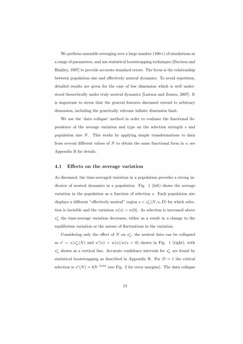
As discussed, the time-averaged variation in a population provides a strong in-
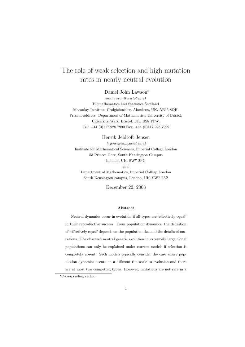
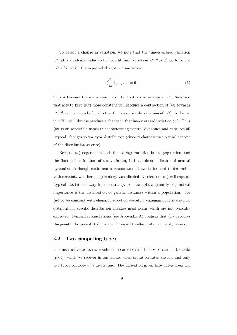
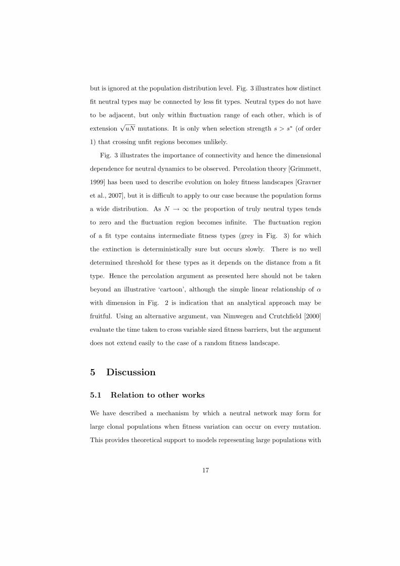
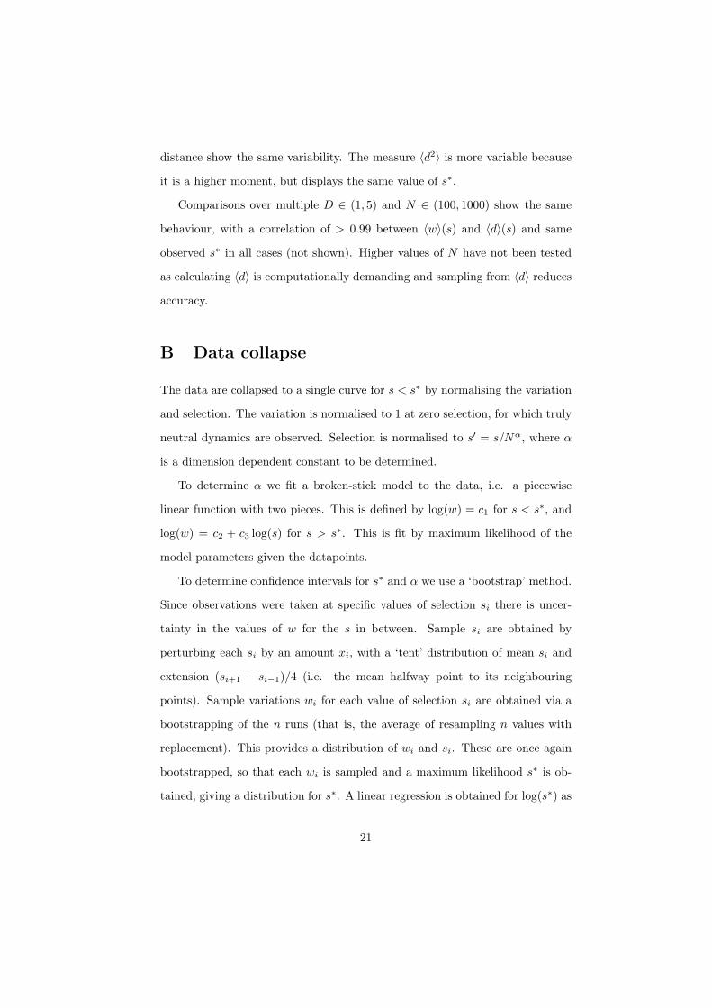
dicator of neutral dynamics in a population. Fig. 1 (left) shows the average
variation in the population as a function of selection s. Each population size
displays a different ”effectively neutral” region s < s∗w(N, u, D) for which selec-
tion is invisible and the variation w(s) = w(0). As selection is increased above
s∗w the time-average variation decreases, either as a result in a change to the
equilibrium variation or the nature of fluctuations in the variation.
Considering only the effect of N on s∗w, the neutral data can be collapsed
as s′ = s/s∗w(N) and w′(s) = w(s)/w(s = 0) shown in Fig. 1 (right), with
s∗w shown as a vertical line. Accurate confidence intervals for s∗w are found by
statistical bootstrapping as described in Appendix B. For D = 1 the critical
selection is s∗(N) = 8N−0.94 (see Fig. 2 for error margins). The data collapse
13
is intended only for s < s∗, though in this case holds over the whole parameter
region. The region s > s∗ corresponds to non-neutral dynamics. The critical
selection observed via a change in the average variation is of the general form:
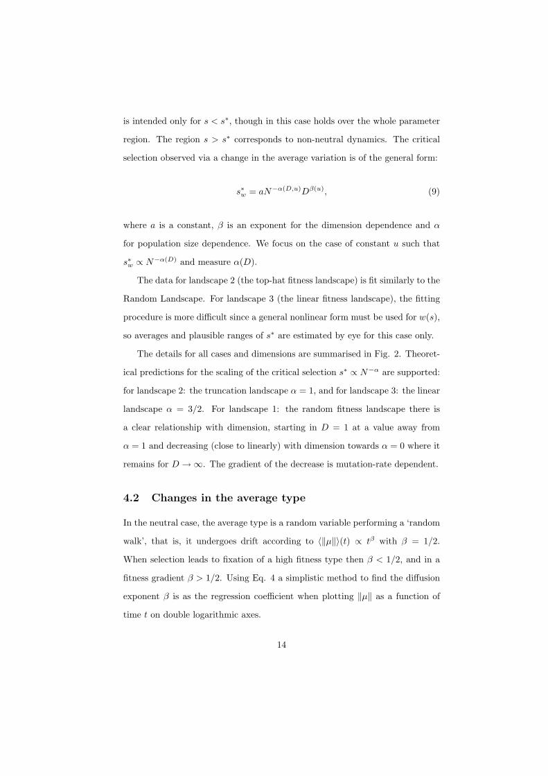
s∗w = aN−α(D,u)Dβ(u), (9)
where a is a constant, β is an exponent for the dimension dependence and α
for population size dependence. We focus on the case of constant u such that
s∗w ∝ N−α(D) and measure α(D).
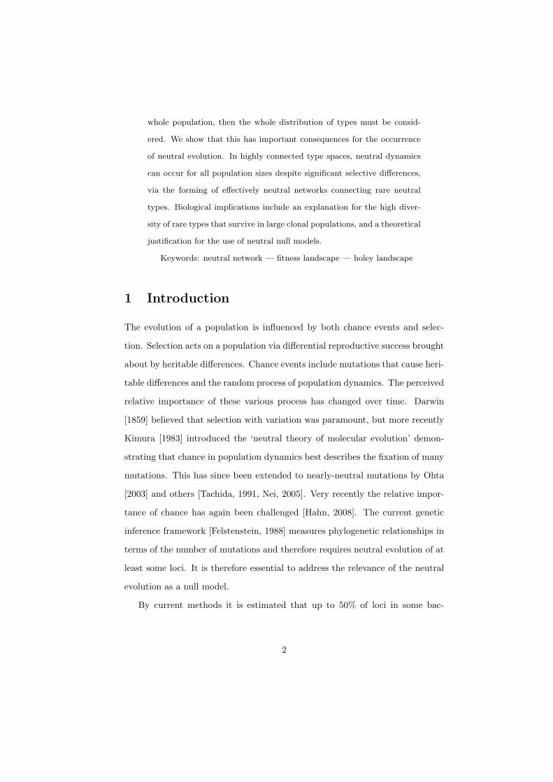
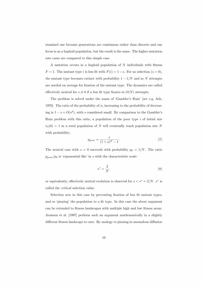
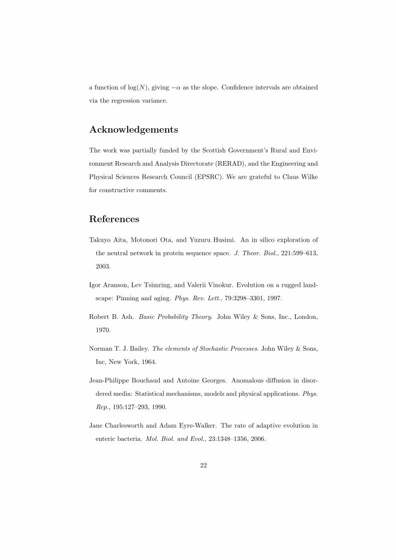
The data for landscape 2 (the top-hat fitness landscape) is fit similarly to the
Random Landscape. For landscape 3 (the linear fitness landscape), the fitting
procedure is more difficult since a general nonlinear form must be used for w(s),
so averages and plausible ranges of s∗ are estimated by eye for this case only.
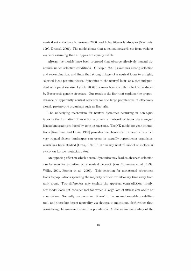
The details for all cases and dimensions are summarised in Fig. 2. Theoret-
ical predictions for the scaling of the critical selection s∗ ∝ N−α are supported:
for landscape 2: the truncation landscape α = 1, and for landscape 3: the linear
landscape α = 3/2. For landscape 1: the random fitness landscape there is
a clear relationship with dimension, starting in D = 1 at a value away from
α = 1 and decreasing (close to linearly) with dimension towards α = 0 where it
remains for D →∞. The gradient of the decrease is mutation-rate dependent.
4.2 Changes in the average type
In the neutral case, the average type is a random variable performing a ‘random
walk’, that is, it undergoes drift according to 〈‖µ‖〉(t) ∝ tβ with β = 1/2.
When selection leads to fixation of a high fitness type then β < 1/2, and in a
fitness gradient β > 1/2. Using Eq. 4 a simplistic method to find the diffusion
exponent β is as the regression coefficient when plotting ‖µ‖ as a function of
time t on double logarithmic axes.
14
The evolution of a population in a random fitness landscape is related to the
behaviour of a random walker in a random potential. Studying this numerically
is notoriously difficult [Bouchaud and Georges, 1990] and the above method
poorly captures the asymptotic behaviour. However, the short and medium
time scales that are of relevance to biological evolution are captured in β as
measured by the above regression method.
As expected from Eq. 4, β = 1/2 is observed for neutral dynamics as seen
for all selection strengths s < s∗µ (not shown). The critical selection observed
s∗µ in the mean position has the form
s∗µ = bDγ(u), (10)
for some constant b and exponent γ, with no dependence on population size N
for all N ≥ 500.
4.3 Variation as the important measure
Using the definition of s∗ = min(s∗w, s∗µ) and Equations 9 and 10, the dynamics of
the mean type provide an important constraint on neutral dynamics if s∗µ < s∗w.
By rearrangement:
α log(N) + (γ − β) log(D) < [log(a)− log(b)]. (11)
Therefore the signs of (γ − β) and [log(a)− log(b)] determine which constraint
holds as N and D become large. By regression in the dimension variable D,
these are empirically observed as positive over all tested parameter values. For
example, at u = 0.05 in the random landscape (γ−β) = 4.5± 0.7 and [log(a)−log(b)] = 6.9 ± 0.8. The signs of the combined constants imply all terms in
Equation 11 are positive. Therefore at low N and D a change in the mutational
15
drift rate can be observed before the population distribution changes shape.
However, if N → ∞ or D → ∞ then s∗w < s∗µ and s∗ = s∗w, i.e. we need only
observe the time-averaged variation.
4.4 Interpreting the results
A statistical description of neutral evolution was used to characterise the effect
of selection on a population distribution. This defined a ‘neutral regime’ in
which the population as a whole evolved effectively neutrally.
For low mutation rates Nu ¿ 1 all individuals are distributed over a maxi-
mum of two types that compete with each other. In this case neutral dynamics
are observed for s < s∗ ∝ N−α with α = 1, as is found in classical models. This
occurs regardless of the distribution of fitter types in the fitness landscape.
For high mutation rates Nu ≥ 1 the population forms a distribution over
many types. The relevant selection parameter s measures the maximum range
of fitnesses experienced by the population. Fitness landscapes with a single
maxima (Eq. 2), or with long range trends (Eq. 3 with s redefined as sdiff) also
have critical selection s∗ ∝ N−α with α = 1. However, fitness landscapes with
large fluctuations but no long distance trend (Eq. 1) allow neutral dynamics
to be observed for a larger range of population sizes N . In suitably connected
fitness landscapes such as that of genotypes (D → ∞) there is no effect of
population size on the critical selection strength s∗. When selection is below s∗,
taking the limit N → ∞ results in a neutral model. The uncorrelated random
fitness landscape is important because correlated random landscapes tend (as
1/√
N) to uncorrelated ones as N →∞.
In the neutral regime for high mutation rates, the population contains a
large number of types with differing fitness. The fitness difference may be large
enough to be measured as selectively important at the level of single mutations,
16
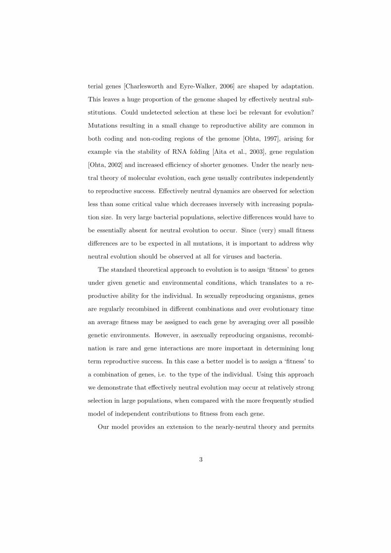
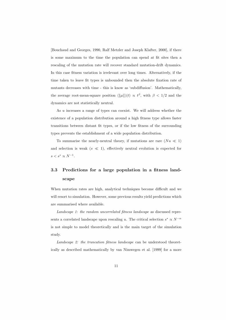
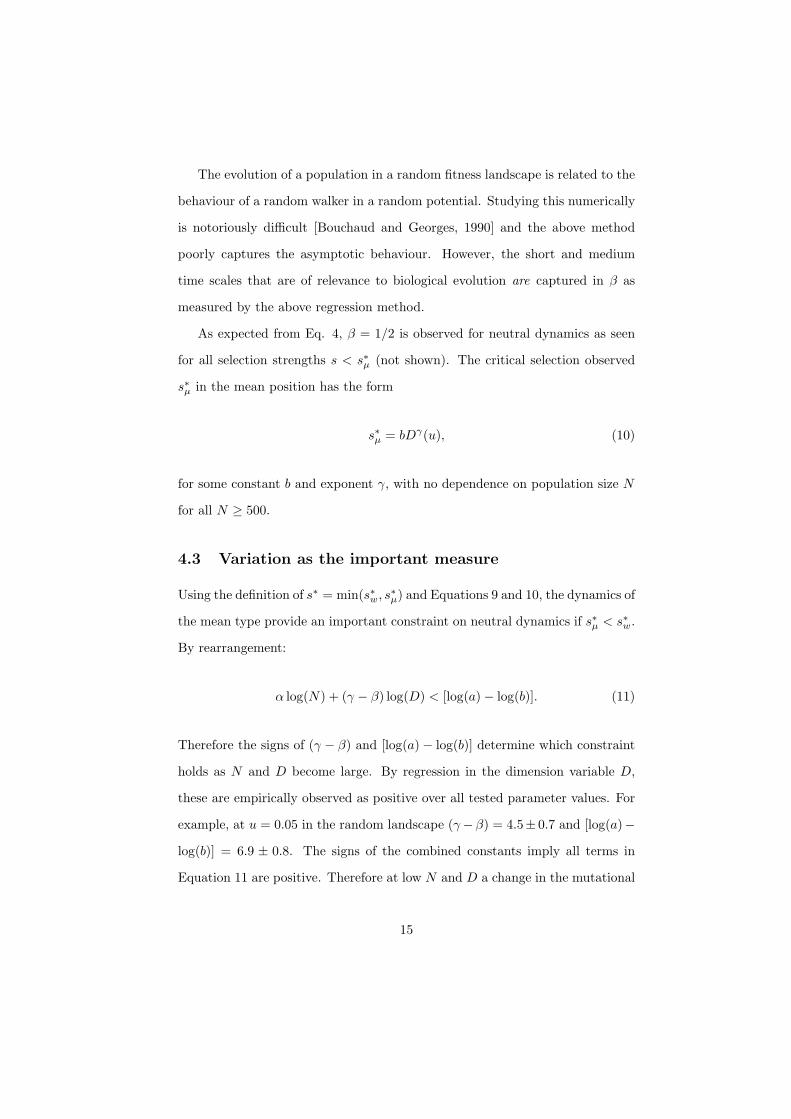
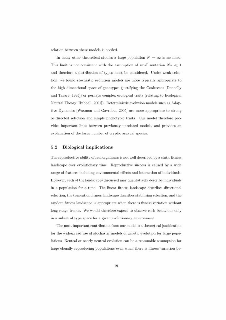
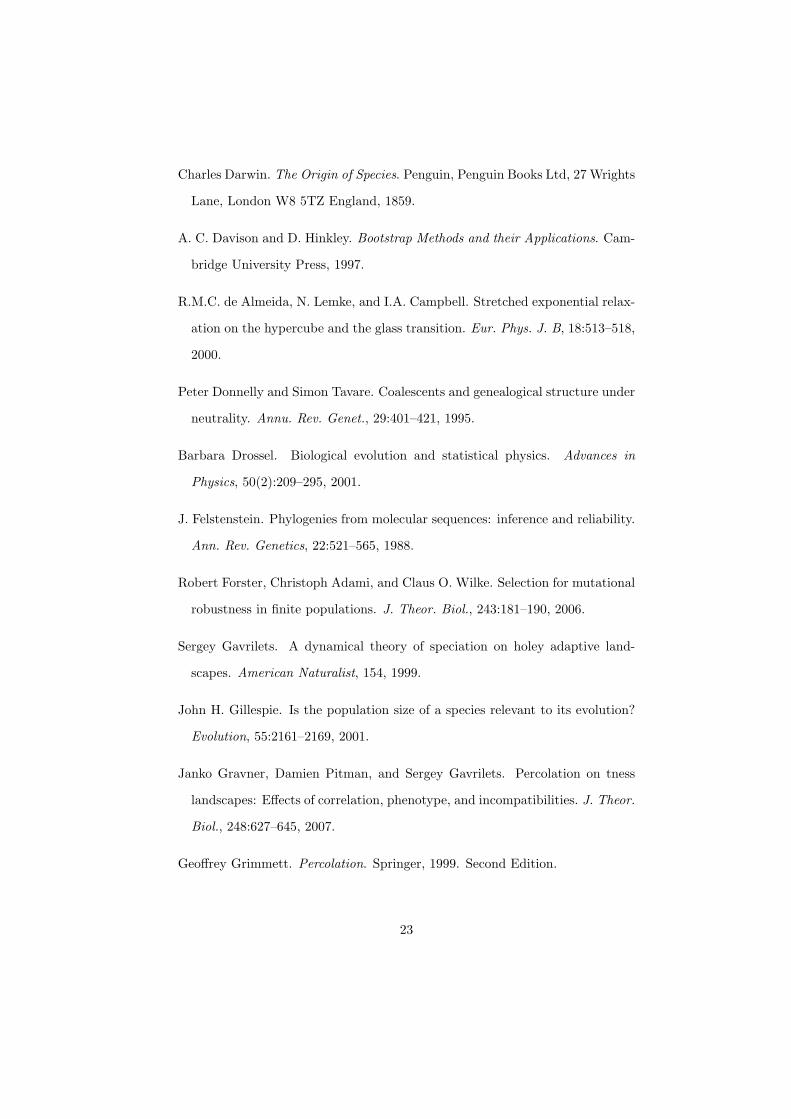
but is ignored at the population distribution level. Fig. 3 illustrates how distinct
fit neutral types may be connected by less fit types. Neutral types do not have
to be adjacent, but only within fluctuation range of each other, which is of
extension√
uN mutations. It is only when selection strength s > s∗ (of order
1) that crossing unfit regions becomes unlikely.
Fig. 3 illustrates the importance of connectivity and hence the dimensional
dependence for neutral dynamics to be observed. Percolation theory [Grimmett,
1999] has been used to describe evolution on holey fitness landscapes [Gravner
et al., 2007], but it is difficult to apply to our case because the population forms
a wide distribution. As N → ∞ the proportion of truly neutral types tends
to zero and the fluctuation region becomes infinite. The fluctuation region
of a fit type contains intermediate fitness types (grey in Fig. 3) for which
the extinction is deterministically sure but occurs slowly. There is no well
determined threshold for these types as it depends on the distance from a fit
type. Hence the percolation argument as presented here should not be taken
beyond an illustrative ‘cartoon’, although the simple linear relationship of α
with dimension in Fig. 2 is indication that an analytical approach may be
fruitful. Using an alternative argument, van Nimwegen and Crutchfield [2000]
evaluate the time taken to cross variable sized fitness barriers, but the argument
does not extend easily to the case of a random fitness landscape.
5 Discussion
5.1 Relation to other works
We have described a mechanism by which a neutral network may form for
large clonal populations when fitness variation can occur on every mutation.
This provides theoretical support to models representing large populations with
17
neutral networks [van Nimwegen, 2006] and holey fitness landscapes [Gavrilets,
1999, Drossel, 2001]. The model shows that a neutral network can form without
a-priori assuming that all types are equally viable.
Alternative models have been proposed that observe effectively neutral dy-
namics under selective conditions. Gillespie [2001] examines strong selection
and recombination, and finds that strong linkage of a neutral locus to a highly
selected locus permits neutral dynamics at the neutral locus at a rate indepen-
dent of population size. Lynch [2006] discusses how a similar effect is produced
by Eucaryotic genetic structure. Our result is the first that explains the prepon-
derance of apparently neutral selection for the large populations of effectively
clonal, prokaryotic organisms such as Bacteria.
The underlying mechanism for neutral dynamics occurring in non-equal
types is the formation of an effectively neutral network of types via a rugged
fitness landscape produced by gene interactions. The NK model for gene interac-
tions [Kauffman and Levin, 1987] provides one theoretical framework in which
very rugged fitness landscapes can occur in sexually reproducing organisms,
which has been studied [Ohta, 1997] in the nearly neutral model of molecular
evolution for low mutation rates.
An opposing effect in which neutral dynamics may lead to observed selection
can be seen for evolution on a neutral network [van Nimwegen et al., 1999,
Wilke, 2001, Forster et al., 2006]. This selection for mutational robustness
leads to populations spending the majority of their evolutionary time away from
unfit areas. Two differences may explain the apparent contradiction: firstly,
our model does not consider loci for which a large loss of fitness can occur on
a mutation. Secondly, we consider ‘fitness’ to be an unobservable modelling
tool, and therefore detect neutrality via changes to mutational drift rather than
considering the average fitness in a population. A deeper understanding of the
18
relation between these models is needed.
In many other theoretical studies a large population N → ∞ is assumed.
This limit is not consistent with the assumption of small mutation Nu ¿ 1
and therefore a distribution of types must be considered. Under weak selec-
tion, we found stochastic evolution models are more typically appropriate to
the high dimensional space of genotypes (justifying the Coalescent [Donnelly
and Tavare, 1995]) or perhaps complex ecological traits (relating to Ecological
Neutral Theory [Hubbell, 2001]). Deterministic evolution models such as Adap-
tive Dynamics [Waxman and Gavrilets, 2005] are more appropriate to strong
or directed selection and simple phenotypic traits. Our model therefore pro-
vides important links between previously unrelated models, and provides an
explanation of the large number of cryptic asexual species.
5.2 Biological implications
The reproductive ability of real organisms is not well described by a static fitness
landscape over evolutionary time. Reproductive success is caused by a wide
range of features including environmental effects and interaction of individuals.
However, each of the landscapes discussed may qualitatively describe individuals
in a population for a time. The linear fitness landscape describes directional
selection, the truncation fitness landscape describes stabilising selection, and the
random fitness landscape is appropriate when there is fitness variation without
long range trends. We would therefore expect to observe each behaviour only
in a subset of type space for a given evolutionary environment.
The most important contribution from our model is a theoretical justification
for the widespread use of stochastic models of genetic evolution for large popu-
lations. Neutral or nearly neutral evolution can be a reasonable assumption for
large clonally reproducing populations even when there is fitness variation be-
19
tween types. It is important to integrate the effects of large mutation rates and
high population sizes into the current theoretical frameworks. Although pop-
ulation size cannot be inferred from genetics data alone [Stephens, 2007] our
model demonstrates that the qualitative nature of dynamics need not change
with population size. Hence stochastic models for changing population sizes
experiencing weak selection are also reasonable. Our model is not directly ap-
plicable to genetics data, but does translate conceptually to problems involving
mutation of DNA. Neutral dynamics may naturally occur under different se-
lective conditions for recombining and non-recombining areas, which may be
important to inference about mitochondrial DNA [William et al., 1995, Rand
et al., 1994] and the Y chromosome (e.g. [Handley et al., 2006]).
The most useful model of biological evolution will differ from situation to
situation, particularly depending on the speed of recombination. Our model
best describes low recombination rates and therefore asexual populations. It
predicts that neutral dynamics can persist for much larger selection strength and
population sizes than standard models for sexual species predict. This explains
the existence of cryptic asexual species. The conditions required for our model
are that mutation rate is not small compared to the inverse population size,
and that genes interact to determine fitness. In this case a surprisingly ‘large’
selective advantage may be present in a population and neutral dynamics can
still be observed.
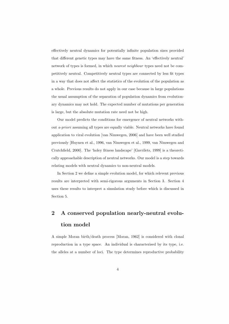
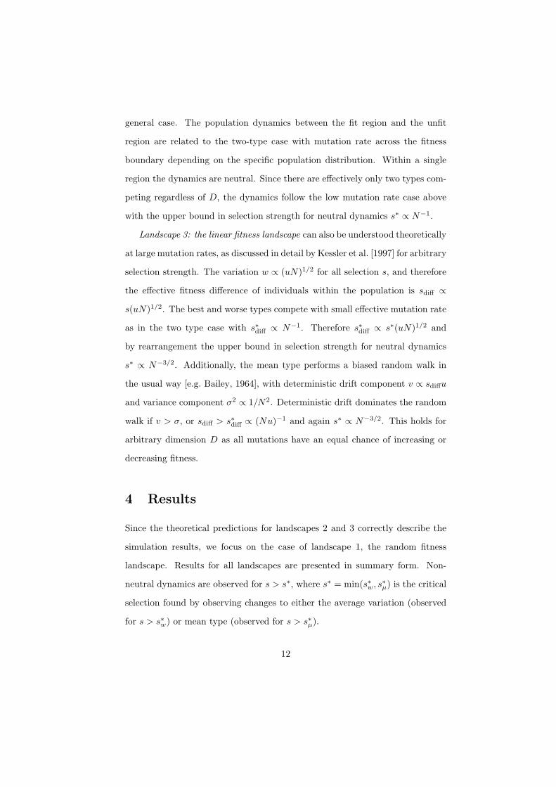
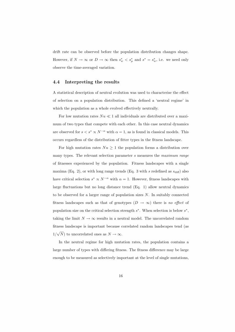
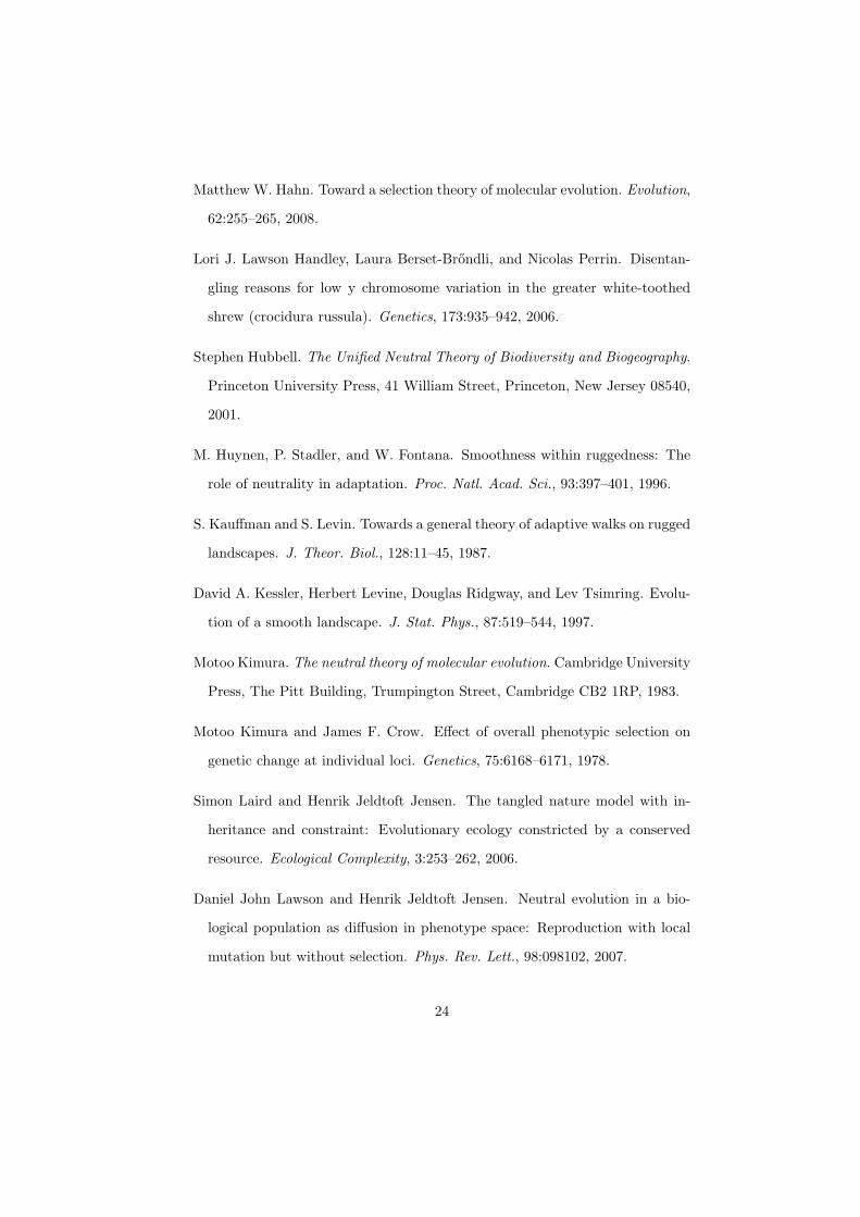
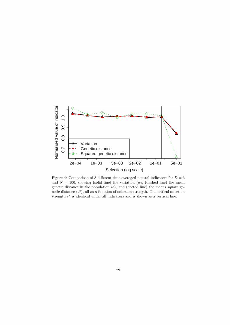
A Genetic distance within the population
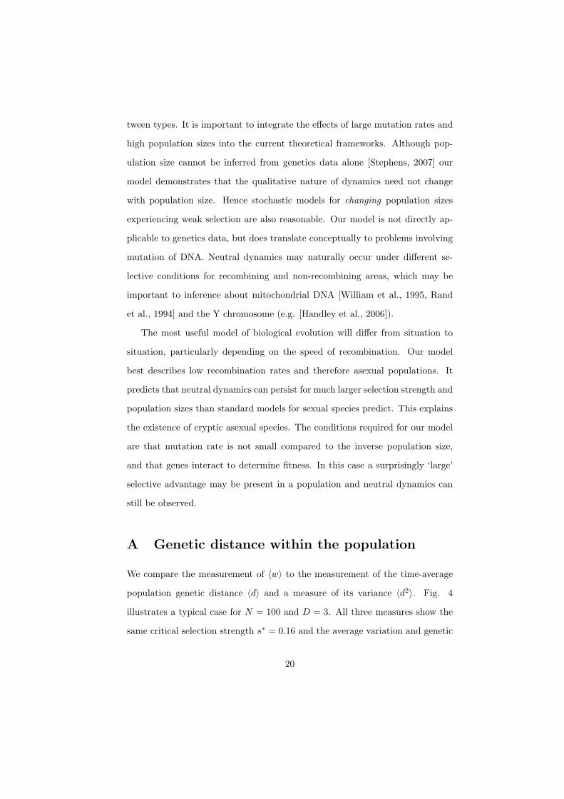
We compare the measurement of 〈w〉 to the measurement of the time-average
population genetic distance 〈d〉 and a measure of its variance 〈d2〉. Fig. 4
illustrates a typical case for N = 100 and D = 3. All three measures show the
same critical selection strength s∗ = 0.16 and the average variation and genetic
20
distance show the same variability. The measure 〈d2〉 is more variable because
it is a higher moment, but displays the same value of s∗.
Comparisons over multiple D ∈ (1, 5) and N ∈ (100, 1000) show the same
behaviour, with a correlation of > 0.99 between 〈w〉(s) and 〈d〉(s) and same
observed s∗ in all cases (not shown). Higher values of N have not been tested
as calculating 〈d〉 is computationally demanding and sampling from 〈d〉 reduces
accuracy.
B Data collapse
The data are collapsed to a single curve for s < s∗ by normalising the variation
and selection. The variation is normalised to 1 at zero selection, for which truly
neutral dynamics are observed. Selection is normalised to s′ = s/Nα, where α
is a dimension dependent constant to be determined.
To determine α we fit a broken-stick model to the data, i.e. a piecewise
linear function with two pieces. This is defined by log(w) = c1 for s < s∗, and
log(w) = c2 + c3 log(s) for s > s∗. This is fit by maximum likelihood of the
model parameters given the datapoints.
To determine confidence intervals for s∗ and α we use a ‘bootstrap’ method.
Since observations were taken at specific values of selection si there is uncer-
tainty in the values of w for the s in between. Sample si are obtained by
perturbing each si by an amount xi, with a ‘tent’ distribution of mean si and
extension (si+1 − si−1)/4 (i.e. the mean halfway point to its neighbouring
points). Sample variations wi for each value of selection si are obtained via a
bootstrapping of the n runs (that is, the average of resampling n values with
replacement). This provides a distribution of wi and si. These are once again
bootstrapped, so that each wi is sampled and a maximum likelihood s∗ is ob-
tained, giving a distribution for s∗. A linear regression is obtained for log(s∗) as
21
a function of log(N), giving −α as the slope. Confidence intervals are obtained
via the regression variance.
Acknowledgements
The work was partially funded by the Scottish Government’s Rural and Envi-
ronment Research and Analysis Directorate (RERAD), and the Engineering and
Physical Sciences Research Council (EPSRC). We are grateful to Claus Wilke
for constructive comments.
References
Takuyo Aita, Motonori Ota, and Yuzuru Husimi. An in silico exploration of
the neutral network in protein sequence space. J. Theor. Biol., 221:599–613,
2003.
Igor Aranson, Lev Tsimring, and Valerii Vinokur. Evolution on a rugged land-
scape: Pinning and aging. Phys. Rev. Lett., 79:3298–3301, 1997.
Robert B. Ash. Basic Probability Theory. John Wiley & Sons, Inc., London,
1970.
Norman T. J. Bailey. The elements of Stochastic Processes. John Wiley & Sons,
Inc, New York, 1964.
Jean-Philippe Bouchaud and Antoine Georges. Anomalous diffusion in disor-
dered media: Statistical mechanisms, models and physical applications. Phys.
Rep., 195:127–293, 1990.
Jane Charlesworth and Adam Eyre-Walker. The rate of adaptive evolution in
enteric bacteria. Mol. Biol. and Evol., 23:1348–1356, 2006.
22
Charles Darwin. The Origin of Species. Penguin, Penguin Books Ltd, 27 Wrights
Lane, London W8 5TZ England, 1859.
A. C. Davison and D. Hinkley. Bootstrap Methods and their Applications. Cam-
bridge University Press, 1997.
R.M.C. de Almeida, N. Lemke, and I.A. Campbell. Stretched exponential relax-
ation on the hypercube and the glass transition. Eur. Phys. J. B, 18:513–518,
2000.
Peter Donnelly and Simon Tavare. Coalescents and genealogical structure under
neutrality. Annu. Rev. Genet., 29:401–421, 1995.
Barbara Drossel. Biological evolution and statistical physics. Advances in
Physics, 50(2):209–295, 2001.
J. Felstenstein. Phylogenies from molecular sequences: inference and reliability.
Ann. Rev. Genetics, 22:521–565, 1988.
Robert Forster, Christoph Adami, and Claus O. Wilke. Selection for mutational
robustness in finite populations. J. Theor. Biol., 243:181–190, 2006.
Sergey Gavrilets. A dynamical theory of speciation on holey adaptive land-
scapes. American Naturalist, 154, 1999.
John H. Gillespie. Is the population size of a species relevant to its evolution?
Evolution, 55:2161–2169, 2001.
Janko Gravner, Damien Pitman, and Sergey Gavrilets. Percolation on tness
landscapes: Effects of correlation, phenotype, and incompatibilities. J. Theor.
Biol., 248:627–645, 2007.
Geoffrey Grimmett. Percolation. Springer, 1999. Second Edition.
23
Matthew W. Hahn. Toward a selection theory of molecular evolution. Evolution,
62:255–265, 2008.
Lori J. Lawson Handley, Laura Berset-Brondli, and Nicolas Perrin. Disentan-
gling reasons for low y chromosome variation in the greater white-toothed
shrew (crocidura russula). Genetics, 173:935–942, 2006.
Stephen Hubbell. The Unified Neutral Theory of Biodiversity and Biogeography.
Princeton University Press, 41 William Street, Princeton, New Jersey 08540,
2001.
M. Huynen, P. Stadler, and W. Fontana. Smoothness within ruggedness: The
role of neutrality in adaptation. Proc. Natl. Acad. Sci., 93:397–401, 1996.
S. Kauffman and S. Levin. Towards a general theory of adaptive walks on rugged
landscapes. J. Theor. Biol., 128:11–45, 1987.
David A. Kessler, Herbert Levine, Douglas Ridgway, and Lev Tsimring. Evolu-
tion of a smooth landscape. J. Stat. Phys., 87:519–544, 1997.
Motoo Kimura. The neutral theory of molecular evolution. Cambridge University
Press, The Pitt Building, Trumpington Street, Cambridge CB2 1RP, 1983.
Motoo Kimura and James F. Crow. Effect of overall phenotypic selection on
genetic change at individual loci. Genetics, 75:6168–6171, 1978.
Simon Laird and Henrik Jeldtoft Jensen. The tangled nature model with in-
heritance and constraint: Evolutionary ecology constricted by a conserved
resource. Ecological Complexity, 3:253–262, 2006.
Daniel John Lawson and Henrik Jeldtoft Jensen. Neutral evolution in a bio-
logical population as diffusion in phenotype space: Reproduction with local
mutation but without selection. Phys. Rev. Lett., 98:098102, 2007.
24
Michael Lynch. The origins of eukaryotic gene structure. Mol. Biol. Evol., 23:
450–468, 2006.
P. A. P. Moran. The Statistical Processes of Evolutionary Theory. Clarendon
Press, Oxford, 1962.
Masatoshi Nei. Selectionism and neutralism in molecular evolution. Mol. Biol.
and Evol., 22:2318–2342, 2005.
Tomoko Ohta. The meaning of near-neutrality at coding and non-coding regions.
Gene, 205:261–267, 1997.
Tomoko Ohta. Near-neutrality in evolution of genes and gene regulation. Proc.
Nat. Acad. Sci., 99:16134–16137, 2002.
Tomoko Ohta. Origin of the neutral and nearly neutral theories of evolution. J.
Biosci., 28:371–377, 2003.
Ralf Metzler and Joseph Klafter. The random walk’s guide to anomalous diffu-
sion: a fractional dynamics approach. Phys. Rep., 339:1–77, 2000.
D. M. Rand, M. Dorfsman, and L. M. Kann. Neutral and non-neutral evolution
of drosophila mitochondrial dna. Genetics, 138:741–756, 1994.
M. Stephens. Inference under the coalescent. In D. J. Balding, M. Bishop, and
C. Cannings, editors, Handbook of Statistical Genetics, 3rd Ed. John Wiley
& Sons, Inc., 2007.
Hidenori Tachida. A Study on a Nearly Neutral Model in Finite Populations.
Genetics, 128:183–192, 1991.
Arne Traulsen, Jens Christian Claussen, and Christoph Hauert. Coevolutionary
dynamics in large, but finite populations. Phys. Rev. E, 74:011901, 2006.
25
Erik van Nimwegen. Influenza escapes immunity along neutral networks. Sci-
ence, pages 1884–1886, 2006.
Erik van Nimwegen and James P. Crutchfield. Metastable evolutionary dynam-
ics: Crossing fitness barriers or escaping via neutral paths? Bul. Math. Biol.,
62:799–848, 2000.
Erik van Nimwegen, James P. Crutchfield, and Martijn Huynen. Neutral evo-
lution of mutational robustness. Proc. Nat. Acad. Sci., 96:9716–9720, 1999.
D. Waxman and S. Gavrilets. 20 questions on adaptive dynamics. J. Evol. Biol.,
18:1139–1154, 2005.
Claus O. Wilke. Adaptive evolution on neutral networks. Bul. Math. Biol., 63:
715730, 2001.
Claus O. Wilke, Paulo R. A. Campos, and Jose F. Fontanari. Genealogical
process on a correlated fitness landscape. J. Exp. Zool. (Mol. Dev. Evol.),
294:274284, 2002.
J. William, O. Ballard, and Martin Kreitman. Is mitochondrial dna a strictly
neutral marker? Trends in Ecology and Evolution, 10:485–488, 1995.
Yi-Cheng Zhang, Maurizio Serva, and Mikhail Polikarpov. Diffusion Reproduc-
tion Processes. J. Stat. Phys., 58:849–861, 1990.
26
Selection
Ave
rage
Var
iatio
n
1e−6 1e−4 1e−2 1
1020
3040
5060
Normalised Selection
Nor
mal
ised
Ave
rage
Var
iatio
n
N= 100N= 500N= 1000N= 2000N= 5000N= 10000
1e−4 1e−2 1 1e+21e−2
0.1
0.2
0.5
1.0
Figure 1: Ensemble averaged variation against selection for fitness landscape1 (random and uncorrelated) as described by Eq. 1 with mutation probabilityu = 0.5 and dimension D = 1, for a range of population sizes N . Left: Ensembleaveraged variation against selection. Each curve is flat for s < s∗w(N) i.e. w(s <s∗w) = w(0). Right: The normalised variation against normalised selection forthe same data, collapsed using the method from the Appendix. The criticalselection s∗w ∝ N−0.94 is shown as a vertical line as an aid to the eye. Eachdatapoint is the time average (over 50000 generations) of a simulation afterit has reached equilibrium, ensemble averaged over 200 independent runs withstandard deviations calculated using statistical bootstrapping.
1 2 3 4 5
0.0
0.5
1.0
1.5
Dimension D
Sca
ling
Exp
onen
tα
Random fitness; p=0.5Random fitness; p=0.05Top hat fitness; p=0.5Linear Landscape
Figure 2: Exponent α for the population size dependence s∗w ∝ N−α as afunction of dimension. Error bars are 95% confidence intervals for the regressionfit for α (linear regression on a log-log scale for selection s against populationN). Shown are the data the for random fitness landscape (Eq. 1) at u = 0.5 andu = 0.05, the ‘top-hat’ correlated fitness landscape (Eq. 2), and the linear fitnesslandscape (Eq. 3). Dashed lines correspond to theoretical values. Horizontalperturbations to the dimension have been made for visibility and do not reflectfractal dimensions.
27
0 5 10 15 20
010
2030
40
s=0.02
0 5 10 15 20
010
2030
40
s=0.04
0 5 10 15 20
010
2030
40
s=0.08
Type Space Direction 1
Typ
e S
pace
Dire
ctio
n 2
Figure 3: Illustration of ‘connectivity’ in the random landscape model (Eq. 1)for D = 2 and N = 100. The fitness landscape itself is shown. Selection valuesare (left) s = 0.02, (middle) s = 0.04 and (right) s = 0.08. Types with fitness inthe range (0.99, 1) compete truly neutrally and are shown in black. Types in greyhave fitness in the range (0.98, 0.99) which is high enough to survive by chancefor moderate times at low population levels. The low mutation rate neutralregime (left) is characterised by a connected network of neutrally competingtypes (coloured black). However, the neutral regime considered in this paper(middle) allows linking of neutrally competing types by slightly less fit types(coloured grey). At higher selection, connectivity breaks down into isolatedclusters and non-neutral dynamics are observed (right).
28
2e−04 1e−03 5e−03 2e−02 1e−01 5e−01
0.7
0.8
0.9
1.0
Selection (log scale)
Nor
mal
ised
val
ue o
f ind
icat
or
VariationGenetic distanceSquared genetic distance
Figure 4: Comparison of 3 different time-averaged neutral indicators for D = 3and N = 100, showing (solid line) the variation 〈w〉, (dashed line) the meangenetic distance in the population 〈d〉, and (dotted line) the means square ge-netic distance 〈d2〉, all as a function of selection strength. The critical selectionstrength s∗ is identical under all indicators and is shown as a vertical line.
29