The scientific legacy of Harold Edwin Hurst (1880 – 1978)

P.E. O’Connell1, D. Koutsoyiannis2, H. F. Lins3, Y. Markonis2, A. Montanari4 & T. Cohn3

1Newcastle University, Newcastle upon Tyne, United Kingdom

Enda.OConnell@newcastle.ac.uk

2National Technical University of Athens, Athens, Greece

3U.S. Geological Survey, Reston, Virginia, USA

4University of Bologna, Bologna, Italy

Abstract

Emanating from his remarkable characterization of long-term variability in geophysical

records in the early 1950s, Hurst’s scientific legacy to hydrology and other disciplines is

explored. A statistical explanation of the so-called ‘Hurst Phenomenon’ did not emerge until

1968 when Mandelbrot and co-authors proposed fractional Gaussian noise based on the

hypothesis of infinite memory. A vibrant hydrological literature ensued where alternative

modelling representations were explored and debated eg ARMA models, the Broken Line

model, shifting mean models with no memory, FARIMA models, and Hurst-Kolmogorov

dynamics, acknowledging a link with the work of Kolmogorov in 1940.

The diffusion of Hurst’s work beyond hydrology is summarized by discipline and citations,

showing that he arguably has the largest scientific footprint of any hydrologist in the last

century. Its particular relevance to the modelling of long-term climatic variability in the era

of climate change is discussed. Links to various long-term modes of variability in the climate

system, driven by fluctuations in sea surface temperatures and ocean dynamics, are

explored. A physical explanation of the Hurst Phenomenon in hydrology remains as a

challenge for future research.

Key words Hurst, Hurst phenomenon, long-term persistence, fractional Gaussian noise,

Hurst-Kolmogorov dynamics, climatic variability

1. Introduction

In 1951, Harold Edwin Hurst published a paper in the Transactions of the American Society

of Civil Engineers (Hurst, 1951) that was to become one of the most influential and highly

cited papers in the field of scientific hydrology; this was supplemented by two more (but

less widely cited) papers; one in the Proceedings of the British Institution of Civil Engineers

(Hurst, 1956), and one in Nature (Hurst, 1957). His unique characterization of long term

variability in Nile flow records and other geophysical time series, based on remarkable

scientific insight, and years of pain-staking data analysis in pre-computer days (Sutcliffe et

al., this issue), revealed that hydrological and other geophysical time series exhibited

statistical behaviour that could not be reconciled with the then prevailing theory (Hurst,

1951). This finding, which came to be known as the Hurst Phenomenon, intrigued

hydrologists and statisticians alike, and a mathematical/statistical framework that could

explain it was not to emerge until some fifteen years later, even though Kolmogorov (1940)

had laid down its mathematical foundation, which however was totally unknown to Hurst

and to the hydrological and statistical communities.

However, Hurst’s methodology and finding have not only continued to inspire further

research by hydrologists worldwide up to the present day, but has influenced developments

in many other fields of science, notably climate science, and has been cited in papers on

such disparate subjects as the analysis of internet traffic and the flow of blood in human

arteries. This extensive dissemination is characterized here by the knowledge tree in

Figure 1 where the ‘branches’ correspond to the broad fields of science where Hurst’s work

and references thereto have been cited; the ‘trunk’ of the tree represents the central role

that hydrology occupies in this dissemination process. It is a further mark of distinction that

the large scale ‘export’ from hydrology to other fields represented in Figure 1 has

characterized Hurst’s research, as hydrology is so often an importer of statistical/stochastic

methods from other fields.

Here, we chronicle the research that has evolved from Hurst’s remarkable finding, dealing

first with the early search for a statistical explanation of the Hurst Phenomenon in the

period 1951 up to 1968, when Mandelbrot and Van Ness (1968) unveiled fractional

Brownian Motion and demonstrated that its increments, fractional Gaussian noise (fGn),

had the necessary attributes to account for the Hurst Phenomenon (Mandelbrot and Wallis,

1968) (Section 2). An upsurge in research followed in which the statistical properties of fGn

were explored further, and where alternative hypotheses and models were proposed and

explored. New insights and advances have resulted from more recent research into the

properties of Hurst-Kolmogorov dynamics (Section 3). Physical mechanisms that could give

rise to the Hurst Phenomenon are explored in Section 4, with the climate system being the

main physical context. Hurst’s legacy to other scientific disciplines is summarized in Section

5, while the case for basing climate risk assessments on the stochastic modelling tools

spawned by Hurst’s original finding is articulated in Section 6. Some conclusions are added

in Section 7, followed by a Tribute and Epilogue.

2. The early era of the Hurst Phenomenon

2.1 Hurst’s Law and the Hurst Phenomenon

Hurst’s extensive studies of long-term fluctuations in the annual flows of the River Nile and

various climatic and geophysical records have been reviewed in detail in a companion paper

by Sutcliffe et al. (2015). For some 900 annual time series comprising streamflow and

precipitation records, stream and lake levels, Hurst established the following relationship,

referred to as Hurst’s Law:

/ ~ (1)

where is referred to as the adjusted range of cumulative departures of a time series of n

values (Table 1), is the standard deviation, / is referred to as the rescaled range of

cumulative departures, and H is a parameter, henceforth referred to as the Hurst coefficient

(the use of H to represent the Hurst coefficient has become standard practice in the

literature, although Hurst himself never used H). Hurst’s interest in estimating long term

reservoir storage on the river Nile led to his focus on the range as a statistic that could

provide the basis of a measure of long-term variability in geophysical time series.

To estimate the coefficient H in equation (1), Hurst used the following relationship:

/ = (2)

where K denotes the resulting estimate of the (population) coefficient H, whereupon

) (3)

This estimate is the slope of a line in log-space with a fixed intercept of –K log ; the choice

of ( in equation (3) is discussed below. The estimates ranged from 0.46 to 0.96 with a

mean of 0.729 and a standard deviation of 0.092 for record lengths ranging from 30 – 2000

years.

Hurst (1951) employed some simple coin-tossing experiments to derive the expected value

of for a normal independent process as

(4)

Independently, Feller (1951) used the theory of Brownian motion to derive equation (4),

which is an asymptotic result, but without the assumption of normality. The form of

equation (3) which was used by Hurst to estimate H was apparently suggested by equation

(4) wherein the terms (n/2) appears. Lloyd (1967) subsequently coined the term ‘Hurst

Phenomenon’ to describe the discrepancy between Hurst’s average value of 0.73 for H and

the theoretical value of 0.5 deduced from classical statistical theory.

2.2 Early attempts to explain the Hurst Phenomenon

The discrepancy between Hurst’s extraordinarily well documented finding from data

analysis and his and Feller’s theoretical result puzzled many statisticians and engineers alike

at the time, and a number of possible explanations were suggested. Hurst (1951) himself

conjectured that non-randomness/long-term persistence as evidenced by the tendency in

geophysical time series for high values to follow high values and low values to follow low

values might be a possible explanation. In a notable contribution, Langbein (1956), in a

discussion of Hurst’s (1956) paper, reinforced Hurst’s work with the observation that the

variance of the sample mean for Hurst’s data was larger than if the data were independent

random, and could be approximated by the relationship

= (5)

where is the standard deviation of subsample means. This implied

= (6)

Note that the mean value of the exponent K, 0.729, derived by Hurst (1951), and Langbein’s

estimate of H = 0.72 derived from equations (5) and (6), are slightly inconsistent; this is

probably due to the different estimation procedures they used. Langbein also deduced that

skewness was an unlikely explanation, as was autocorrelation of a Markovian nature. He

suggested that the persistence in Hurst’s data was of a more complex nature.

Feller (1951) suggested that the discrepancy might be accounted for by autocorrelation of a

Markovian nature, but Barnard (1956) disputed this suggestion, commenting that no simple

set of correlations could account for Hurst’s result. In a further notable contribution, Hurst

(1957) reported on some card sampling experiments in which he generated time series of

varying lengths, the longest of which contained 4000 values and which had a mean value of

H = 0.72. Hurst’s sampling procedure was subsequently interpreted by Klemeš (1974) as a

form of ‘shifting mean’ model in which the mean of the process was sampled randomly for

random periods in which values were sampled independently.

Theoretical studies of the different definition of the range (Table 1) were pursued by a

number of statisticians. Anis and Lloyd (1953) derived the expected value of (the

superscript p denotes population, as the definition of implies knowledge of the

population mean) for finite n and independent variates with a common distribution, while

Solari and Anis (1957) derived the same result for for a normal independent process.

However, H = 0.5 was inherent in all of these analyses. This continued to challenge

statisticians such as Moran (1959) who wrote reinforcing Barnard’s earlier (1956)

contention:

‘….the exponent 0.73 could not occur unless the serial dependence was of a very

peculiar kind because with all of the plausible models of serial dependence, the series

of partial sums is approximated by a Bachelier-Wiener process when the time scale or

economic horizon is sufficiently large.’

However, Moran (1964), working with the population range , deduced that for moderate

n, Hurst’s result could after all be explained by skewness, and used highly skewed

distributions with large but finite second moments about the mean (such as a truncated

Cauchy distribution) to justify his argument. He did, however, note that such distributions

were unlikely to provide a good fit to Hurst’s data, and his inferences did not extend to the

rescaled range that was the basis for Hurst’s finding.

In a lucid summary of the work which had been carried out up to that time, Lloyd (1967)

commented as follows:

‘…We are then in one of those situations, so salutary for theoreticians, in which

empirical discoveries stubbornly refuse to accord with theory. All of the researches

described above lead to the conclusion that in the long run, should increase

like , whereas Hurst’s extraordinarily well documented empirical law shows an

increase like where K is about 0.7. We are forced to the conclusion that either the

theorists interpretation of their own work is inadequate or their theories are falsely

based: possibly both conclusions apply.’

Leading stochastic hydrologists of the era fared no better than the theoreticians in

explaining the Hurst Phenomenon. Monte Carlo (MC) simulation studies of the behaviour of

/ were carried out by Matalas and Huzzen (1967) for a lag-one autoregressive

(Markov) process. While extended transients in / could be obtained as the lag one

autocorrelation coefficient increased, the simulated values were locally unrealistically

smooth for annual streamflow, reflecting large lag one autocorrelation coefficients, and

they concluded that their results did not offer a satisfactory explanation. Fiering (1967)

came to a similar conclusion based on simulation experiments with higher order

autoregressive models.

2.3 Fractional Brownian motion and fractional Gaussian noise

The foundations for an explanation of the Hurst Phenomenon were laid by Mandelbrot

(1965), and the theoretical framework was developed fully by Mandelbrot and Van Ness

(1968), who acknowledged that Kolmogorov (1940) had earlier introduced a mathematical

process with such behaviour. By analogy with Brownian motion, they defined fractional

Brownian motion (fBm) as a process in which past, independent increments of

Brownian motion from time -∞ to t are weighted by time lag raised to the

power where H is the Hurst exponent satisfying is a

continuous time stochastic process with self-similar increments such that, if the time-scale is

changed in the ratio T, where the functions - and -

are governed by the same probability law (Mandelbrot and Wallis, 1968). It follows

from this property that

Var [ - = (7)

where is a constant.

A further consequence of self-similarity is that the population range and adjusted

range of the continuous function obey Hurst’s law asymptotically:

[ = (8)

[ = (9)

where and are constants.

The increments

= - (10a)

(10b)

with the kernel function described by

for (11a)

for (11b)

were defined by Mandelbrot and Wallis (1969a) as discrete-time fractional Gaussian noise.

With the assumption that equation (9) holds for the discrete case, and that

implies then the increments of fBm provide the necessary basis for

modelling Hurst’s Law. The process is stationary for , and self-

similar such that

{ } { } (12)

which means that { } and { } have the same joint distribution functions apart from the

scaling constant . Noting that the concept of self-similarity had originated in the theory

of turbulence, Mandelbrot and Wallis (1968) observed that it had become useful in studying

a range of phenomena (Mandelbrot, 1963; 1966; 1967), and suggested that self-similar

models might supersede the current models which could not account for the Hurst

Phenomenon.

The autocovariance function of is (Mandelbrot and Wallis, 1968):

( (13)

which, for a large lag k, can be approximated as

(14)

where is the variance of The summation of does not converge, whereas the

corresponding summation for all autoregressive and autoregressive moving average models

based on the increments of Brownian motion (i.e. white Gaussian noise) is finite. This has

been interpreted as reflecting “infinite memory”, which is in line with the definition of fBm

as a weighted integral of past increments of Brownian motion from to t, with distant

past events having a small but significant influence on current behaviour. Long-term

memory gives rise to long-term persistence (LTP), but LTP can also arise from models with

no memory that are based on equation (13) (section 3.3/3.5). A consequence of the power-

law form of is that realizations of fGn will exhibit a wealth of random low frequency

swings and cycles, similar to the behaviour observed by Hurst in the long-term records

which he analysed. This is also reflected in the spectrum which has the form

(15)

where and .

From equation (7), the variance of the partial sums of discrete time fGn

= (16)

is

Var = (17)

whence

Var (18)

or

(19)

This relationship, as noted above, was derived by Langbein (1956) from Hurst’s data, and

referred to as Langbein’s corollary of Hurst’s law by Mandelbrot and Wallis (1968).

2.4 Fractional Gaussian noise approximations

Computer-based discrete time approximations of fGN require (a) the integral in equation

(10) to be replaced by a weighted sum of a discrete-time white-noise process , and (b) the

interval to be replaced by a finite span where M is a large

enough constant. Mandelbrot and Wallis (1969a) proposed two approximations which they

labeled Type 1 and Type 2. The Type 2 approximation is written as:

= (20)

which is a moving average of M Gaussian independent random increments. The Type 1

approximation employed a finer integration grid and was therefore more accurate but more

computationally intensive.

Mandelbrot and Wallis (1969a,b,c) carried out a series of computer experiments in which

they demonstrated that their fGn approximations obeyed Hurst’s Law (1) with the slope of a

trend line on a Log-Log plot of against for selected in the range

(referred to a ‘pox diagram’) shown to correspond to the value of H used in the fGn

generator. Moreover, they generated highly skewed fGn series and showed that the slopes

of trend lines remained unchanged relative to the Gaussian case, demonstrating the

importance of standardization by in making Hurst’s law robust to skewness, and

demonstrating that earlier attempts to explain the Hurst Phenomenon in terms of skewness,

and based only on , had been fallacious (Mandelbrot and Wallis, 1969d). This finding was

later reinforced by O’Connell (1976). Moreover, they showed that the presence of a periodic

component, such as the annual cycle in sub-annual time series, distorted the

against plot, and inhibited the reliable estimation of H. They also reaffirmed Hurst’s

law for long geophysical records which extended to thousands of years in the case of tree

ring data (Mandelbrot and Wallis, 1969e).

3. From Fractional Brownian Motion to Hurst-Kolmogorov Dynamics

Fractional Gaussian Noise (fGn) and its associated power-law covariance function provided a

new framework for stochastic hydrology which led to an upsurge in research into different

ways of approximating fGn and a renewed search for alternative, and possibly simpler

statistical explanations, of the Hurst Phenomenon. But all of these endeavours were

constrained by the need for (a) a stationary model and (b) one that could approximate

Hurst’s Law at least for long transients, and by implication, a power law or hyperbolic

covariance function.

3.1 Various methods of generating fGn

In response to criticisms of the initial type 1 and type 2 fGn approximations, Mandelbrot

(1971) developed a ‘fast’ fractional noise generator for 0.5 < H < 1. He approximated the

covariance function of fGn using a summation of suitably weighted and independent Gauss-

Markov processes, with the weights and parameters being a function of H. He incorporated

a high frequency Gauss-Markov process which would allow the fitting of the high frequency

characteristics of an observed series as well as the Hurst coefficient.

Recognizing that the initial type 2 approximation yielded values of the lag one

autocorrelation coefficient which were too high to approximate that of fGn as well as

observed annual streamflow, Matalas and Wallis (1971) developed a filtered fGn

approximation by sampling every pth value (i.e. at times p, p > 1). As p increases, the lag one

autocorrelation decreases, this giving a better fGn approximation and the flexibility to fit an

estimated for an observed series. Matalas and Wallis (1971) also developed a multisite

extension of the single site filtered fGn model.

Rodriguez-Iturbe et al. (1972) and Mejia et al. (1972) proposed the Broken Line (BL) model

as a summation of simple BL processes, and showed how it could serve as an approximation

to fGn. By focusing on a link between the second derivative of the autocorrelation function

of the BL process at lag zero and its crossing properties, they suggested an alternative

approach to estimating the long run properties of geophysical time series. They suggested

that generated synthetic time series should preserve a ‘memory’ of a historic time series,

and demonstrated a procedure for doing this using the BL model (Garcia et al., 1972).

Hipel and McLeod (1978a) proposed an exact method of generating an fGn sample of

specified length n based on generating multivariate fGn random variables having an (n × n)

correlation matrix with elements , the autocorrelation function of fGn based on

equation (13). They used a standard Cholesky decomposition of the correlation matrix to

provide the coefficients needed to generate fGn. Here, the span of dependence is n, so it

needs to be suitably large to reproduce the Hurst Phenomenon over a long time span.

3.2 ARMA models

Box and Jenkins (1970) book stimulated widespread interest in the use of autoregressive

moving average (ARMA) models to represent hydrological time series. Heretofore, only

autoregressive models had been used, and ARMA models offered additional flexibility.

O’Connell (1971, 1974a) showed that a simple ARMA(1,1) model:

(21)

with autocorrelation function

(22a)

. (22b)

could provide an alternative representation of the Hurst Phenomenon in comparison to fGn.

For values of close to the stationarity boundary of +1, long transients showing good

agreement with Hurst’s Law were obtained (up to n = 10,000), with slopes varying as a

function of the parameters, while the parameter could be used to control the value of .

The ARMA(1,1) model represents a simple approximation to fGn that reproduces the main

scales of fluctuation underlying Hurst’s Law, although asymptotically, H = 0.5, as is the case

for all fGn approximations. However, formal fGn approximations have the advantage that H

can be prescribed a priori as a model parameter, whereas, for the ARMA (1,1) model, it has

to be estimated a posteriori from simulation experiments.

O’Connell (1974b,1977) investigated the properties of the moment and maximum likelihood

(ML) fitting procedures presented in Box and Jenkins (B&J) (1970) using extensive MC

simulation experiments, and found the resulting estimates to be biased and highly variable

for the parameter ranges explored by O’Connell (1971,1974a) and for the sample sizes

typically available for annual streamflow. As moment fitting used low lag correlations, and

as the likelihood function was based on one step ahead innovations, B&J fitting procedures

were designed primarily for short-term forecasting rather than long-term prediction.

Moreover, the information content of small samples is low in the presence of LTP. In an

effort to overcome these problems, O’Connell (1974b,1977) used MC simulation to derive

tables relating the ARMA(1,1) model parameters to estimated mean values of K (the

estimate of the Hurst coefficient given by equation (2)) and of , for sample sizes of 25, 50

and 100. For a practical application, values of and would then be chosen based on

matching the observed K and estimates with their respective mean values in the tables,

interpolating where necessary. However, sampling variability can mean that getting a

unique match may not be easy.

Wallis and O’Connell (1973) explored the question of whether hydrological records were

long enough to identify, with any degree of confidence, an appropriate model for use in MC

simulation studies of firm reservoir yield. They used MC simulation to show that statistical

tests based on and lacked power in distinguishing between different generating

models, particularly when LTP was present.

Hipel and McLeod (1978b) fitted ARMA models to 23 annual geophysical time series,

ranging in length from n = 96 to 1164 years using their improved methods of model

identification, parameter estimation and diagnostic checking (Hipel et al., 1977). Using MC

simulation and a goodness of fit test, they showed that the fitted models preserved the

historic series estimates of K and , and argued that a fGn model was not needed in

these cases. The series they used were generally much longer than those typically available

in hydrology, thus avoiding the small sample estimation problems discussed above.

3.3 Shifting mean models

In a penetrating discourse on the Hurst Phenomenon, Klemeš (1974) argued that the

concept of infinite memory invoked by fGn was not physically realistic, and posed the

question of what memory length might be plausible for hydrological systems. He first

formulated a shifting mean model based on Gaussian independent synthetic series, whose

mean value was allowed to assume two different values, alternating regularly after constant

intervals of different lengths called epochs; this is very similar to the playing card

experiment performed by Hurst (1957) and to one subsequently developed by Potter

(1975). He then proceeded to show that, by choosing a suitable distribution for epoch

lengths, and sampling the fluctuations in the mean from a Gaussian distribution with

different standard deviations, he was able to reproduce agreement with Hurst’s Law, with

slopes varying as a function of the model parameters. Although he referred to

nonstationarity in the mean throughout the paper, he deduced that his model was

stationary, as he stated that although ‘it was nonstationary by definition, can well be

considered stationary in the sense that its probability laws do not change through time'. He

also showed that transients with Hurst exponents greater than 0.5 could be produced

through repeated cycling of white noise through a semi-infinite storage reservoir. He left

open the question of what physical mechanisms in nature might account for the Hurst

Phenomenon.

Boes and Salas (1978) derived the theoretical properties of a class of stationary shifting

mean models, and showed that one member of the class had an autocorrelation function

identical to that of the ARMA (1,1) model; they derived the relations between the

parameters of the two models. Although a shifting mean model has no memory, its

autocorrelation function reflects the apparent dependence introduced through fluctuations

in the mean that alternate, producing pseudo-trends. Therefore, an autocorrelation

function with a long tail does not necessarily imply long-term memory; it can arise from a

stationary stochastic process with no memory. Based on some simulation experiments with

ARMA (1,1) and shifting mean models, Salas et al. (1979) suggested the Hurst Phenomenon

might be interpreted as a pre-asymptotic behaviour, since long transients could be

simulated. In addition, Ballerini and Boes (1985) showed that certain shifting mean

processes have autocorrelation structures exhibiting long-term dependence, giving rise to

Hurst behaviour.

Bhattacharya et al. (1983) have shown that the Hurst Phenomenon can arise when a

deterministic trend is incorporated into a short memory stochastic process. However, this is

a nonstationary process with a mean which grows indefinitely, and for which there may be

no physical justification.

3.4 FARIMA models

Hosking (1981) and, independently, Granger (1980) and Granger and Joyeaux (1980),

introduced fractionally differenced FARIMA (p,d,q) models with an asymptotic covariance

function

(23)

where d is a fractional differencing parameter satisfying , and p and q are

the orders of the autoregressive and moving average components. By comparing the

exponents in equations (14) and (23), The FARIMA (0,d,0) process is written

as

(24)

where B is the backward difference operator. This leads to an AR process of infinite order:

= (25)

where

(26)

which offers a very convenient method of generating fractional noise with a finite upper

limit in (25); a moving average representation can also be used. Hosking (1981) then

generalized the FARIMA (0,d,0) model to the FARIMA (p,d,q) case. Once the parameter d

has been estimated (e.g. through one of the methods used to estimate H), the well-

developed ARMA estimation methodology can then be applied to the fractionally

differenced series = to estimate the autoregressive and moving average

parameters. This flexible approach has the advantage that it can be used to estimate

explicitly both the short-term and long-term properties of a time series, whereas ARMA

models can only do this implicitly, and asymptotically have H = 0.5 (Hosking, 1984). An

application of the FARIMA approach has been described by Montanari et al. (1997).

Granger (1980) showed that a process defined as the aggregation of a number of lag-one

Markov processes with parameters sampled from a Beta distribution has the covariance

function (13); this aggregation process is analogous to Mandelbrot’s (1971) fast fractional

Gaussian noise generator.

3.5 Hurst-Kolmogorov dynamics

This alternative title to fractional Gaussian noise is justified to give prominence to the work

of Hurst, and to that of Kolmogorov (1940) who, as already mentioned, first proposed the

mathematical form of the process. It signifies further developments related to the Hurst

Phenomenon which appeared more recently, in the 21st century. In a series of papers,

Koutsoyiannis (2002, 2003, 2006a,b, 2011) and Koutsoyiannis and Montanari (2007) have

brought a fresh perspective to the Hurst Phenomenon and scaling behaviour, with a

particular focus on interpreting and modelling ‘change’. Koutsoyiannis (2002) demystified

the previous complex mathematics behind fGn by presenting its essential properties in a

few equations. Firstly, he derived the variance and autocorrelation of a stochastic process

on multiple temporal scales. In particular, he showed that if a Markov (AR(1)) process is

aggregated to higher time scales, it has precisely the same form of autocorrelation function

as an ARMA(1,1) process, while as the time scale increases, this ARMA(1,1) process becomes

indistinguishable from white noise. Moreover, he showed that if fGN is aggregated to a level

j, i.e., j values are summed to give the aggregated process, the autocorrelation function is

independent of j, and is identical to equation (13) when standardized by the variance. This

derives from the self-similarity of fGn. He advocated the use of equation (18) as a more

reliable estimator of H than one based on the rescaled range which is essentially the

approach employed by Langbein (1956) on Hurst’s data. He then suggested that the

modelling of a climate that ‘changes irregularly, for unknown reasons, on all timescales’

(National Research Council, 1991), should be undertaken using a process with multiple

scales of fluctuation and no memory, and showed that such a shifting mean process can be

used to approximate fGn. He then presented three algorithms for generating

approximations to fGn based on (a) a multiple time scale fluctuation approach; (b) a

disaggregation approach and (c) a symmetric moving average approach.

Koutsoyiannis (2003) focused on the problem of modeling a highly variable climate with

indistinguishable contributions from natural climatic variability and greenhouse gas

emissions, and advocated a stochastic modeling approach that respects the Hurst

Phenomenon. Noting that classical statistics are deficient when used to characterize a

highly variable climate, he developed a method of jointly estimating the unknown variance

and Hurst coefficient of a time series. Starting from the relationship (18), the estimation of

and H is based on the following relationships:

(27)

where j is the time scale (ranging from 1 to a maximum value [n/10], with n being the

sample size), and represents a correction to achieve an approximately unbiased

estimator of the standard deviation . A possible approach to estimating H is to use a

regression of ln on ln j to begin with, and then to use the correction iteratively

until convergence is achieved. Koutsoyiannis (2003) advocated a more systematic approach

involving the minimization of an error function:

(28)

where the weight 1/ , p = 1,2… allows decreasing weights to be assigned to increasing

scales where the sample size is smaller. He demonstrated that, for synthetic data generated

with H = 0.8, the new method gave estimates of the variance and H which were unbiased

and with smaller sampling variances than conventional estimators (e.g. equation (2)). He

applied the method to three hydrometeorological time series with lengths ranging from 91

to 992 years, and showed that they were consistent with the assumed scaling hypothesis for

the variance, and Hurst’s law. Moreover, he demonstrated how appropriate hypothesis

testing (e.g. testing for a trend) should be undertaken when the underlying process exhibits

scaling behaviour.

In a further paper, Koutsoyiannis (2006a) argues that long-term trends in hydrological time

series should not be regarded as deterministic components of a hydrological times series,

and therefore indicating nonstationarity, unless there is a clear physical explanation.

Otherwise, such trends are best regarded as parts of irregular long term fluctuations that

underlie the Hurst Phenomenon, and stationary stochastic models obeying Hurst’s Law offer

the best means of quantifying the large hydrological uncertainty for water resources

planning under a highly variable climate.

To gain insight into how the scaling behaviour synonymous with the Hurst Phenomenon

might be generated, Koutsoyiannis (2006b) constructed a toy model that gives traces that

can resemble historical climatic time series. The model is based on a simple dynamical

system representation with feedbacks, as feedbacks are known to exist in the climate

system (Rial et al., 2004); however, the model feedbacks have no physical basis, and simply

act upon the previous value of the process through a transformation to generate the next

value. The model is deterministic and has few parameters, and no inputs or random

components; given suitable values of its parameters and initial conditions, it can mimic the

time evolution of historical climatic series, and their scaling behaviour. However, it is shown

to have no predictive power (except for short lead times), because the dynamics, despite

being simple, is chaotic, a property also found in the climate (Rial et al., 2004).

Koutsoyiannis and Montanari (2007) discuss various approaches to detecting the presence

and intensity of LTP in hydroclimatic time series, which they distinguish from self-similar

scaling which is a model property, and advocate the use of the climacogram (standard

deviation as a function of time scale) over other methods, i.e. based on equation (18)

applied at different time scales. Moreover, they derive measures of the information content

for a simple scaling stochastic process (essentially fGn) with parameter H as

(29)

where is the equivalent or effective sample size in the classical IID sense. Based on this

result, and a sample of 1979 values for the longest temperature record for which they

estimated H, the effective sample is 3 based on (29). This startling result is a reminder that,

in an LTP world, the typical lengths of flow record available are inadequate for such

applications as reservoir yield estimation (Wallis and O’Connell, 1973). Koutsoyiannis and

Montanari (2007) also discuss hypothesis testing for LTP associated with natural climatic

variability and anthropogenic climate change, and demonstrate, for the series that they

analysed, the difficulty of detecting and attributing ‘change’. They cite the case where

Rybski et al. (2006) and Cohn and Lins (2005) focused on the detection and attribution of

climate change, but arrived at essentially opposite conclusions concerning the relative roles

of natural dynamics and anthropogenic effects in explaining recent warming. They conclude

that the available statistical methodologies are not wholly fit-for purpose; indeed, Cohn and

Lins (2005) suggest that “From a practical standpoint…..it may be preferable to acknowledge

that the concept of statistical significance is meaningless when discussing poorly understood

systems”.

Koutsoyiannis (2011) focused initially on the use and misuse of the terms ‘climate change’

and ‘nonstationarity’, and argued that the former is redundant and non-scientific, since the

climate has always undergone change, while the latter, and the alternative, and infinitely

more tractable, concept of stationarity, is frequently misunderstood. He used realizations

from a stationary shifting mean model to make the point that, while an individual realization

may appear nonstationary, the underlying stochastic process is stationary, and there is no

justification for invoking nonstationarity unless there is a clear association with a

deterministic forcing function. He uses a case study of the water supply system for Athens

to demonstrate how the uncertainty over future water availability was quantified using

Hurst-Kolmogorov dynamics, in the absence of credible predictions from General Circulation

Models (GCMs). Interestingly, Sveinsson et al. (2003) have also shown that shifting mean

models can be used to model climatic indices describing atmospheric circulation (e.g. the

Pacific Decadal Oscillation). In the event that credible predictions of future changes (e.g.

associated with known features such as El Nino or greenhouse gas emissions) are available,

then they can be incorporated into the HK approach.

Lins and Cohn (2011) express similar sentiments over stationarity and nonstationarity, but

point out that, if we do not understand the long-term characteristics of hydroclimatic

processes, finding a prudent course of action in water management is difficult. They discuss

three aspects of this problem: HK dynamics, the complications that LTP introduces with

respect to statistical understanding, and the dependence of statistical trend-testing on

arbitrary sampling choices. In these circumstances, they suggest that, since we are ignorant

about some aspects of the future, a prudent approach may be to proceed under well-

established principle of risk aversion and adaptation, and in the absence of a viable

alternative, to keep stationarity alive, rather than consider it “dead” (Milly et al. 2008). This

is advocated by a couple of more recent studies by Koutsoyiannis and Montanari (2014) and

Montanari and Koutsoyiannis (2014); notably, the latter study claims that “stationarity is

immortal”.

4. In Search of a Physical Explanation for the Hurst Phenomenon in

Hydroclimatic Time Series

In seeking a physical explanation of the Hurst Phenomenon, it is necessary to draw a

distinction between mathematical/statistical constructs that can reproduce the required

behaviour in the rescaled range and the climacogram (variance at aggregate time scales),

and an understanding of the physical mechanisms giving rise to the long-term

fluctuations/long-term persistence in hydroclimatic time series. Klemeš (1974) clearly

recognised the distinction between inferring a physical explanation from the structure of a

stochastic model, and seeking to understand the causal physical mechanisms that could give

rise to the Hurst Phenomenon when he wrote in his conclusions:

'It also is only natural and perfectly in order for the mathematician to concentrate on the

formal geometric structure of a hydrologic series, to treat it as a series of numbers and view

it in the context of a set of mathematically consistent assumptions unbiased by the

peculiarities of physical causation. It is, however, disturbing if the hydrologist adopts the

mathematician’s attitude and fails to see that his mission is to view the series in its physical

context, to seek explanations of its peculiarities in the underlying physical mechanism rather

than to postulate the physical mechanism from a mathematical description of these

peculiarities.'

Here, we review the various explanations/mechanisms that have been proposed from the

two standpoints in Klemeš’ quote. We confine ourselves to the hydrological context only, as

each field in which the Hurst Phenomenon has been observed has its own specific context

and possible explanations which are a function of that context.

4.1 Inferring explanatory mechanisms from data and stochastic models

The fGn model was the first stochastic model proposed in the hydrological literature that

could reproduce the Hurst Phenomenon. Its kernel function (11) implies an infinite memory

which, as already noted, was challenged by Klemeš (1974) as physically unreasonable. As

already discussed, long transients can be generated by finite memory ARMA models (e.g.

O’Connell, 1971) and shifting mean models (e.g. Sveinsson et al., 2003) before convergence

to H = 0.5. However, no convergence towards H = 0.5 has been reported in the hydro-

climatic literature. Markonis and Koutsoyiannis (2013) have demonstrated that the Earth’s

temperature is consistent with Hurst behaviour (with H > 0.90) throughout the entire time

window on which the available reconstructions provide information i.e. up to 500 million

years. Therefore, more and more variability emerges as the time window/time scale for data

analysis increases. To model this multi-scale variability, one can either use a memory-based

approach (e.g. the fast fGn generator (Mandelbrot, 1971), or a FARIMA model (Hosking,

1981), or a shifting mean model with no memory (Koutsoyiannis, 2002). These represent

opposite ends of the spectrum in terms of what might be plausible in physical terms, but

both can arguably do the same job in terms of encapsulating the uncertainty implied by the

Hurst phenomenon when it comes to assessing the reliability of water resource systems.

It is not possible to infer which of these two assumptions (or interpretations) might be most

plausible, based on the available data; however, it is important to recognise that long-term

memory cannot be inferred from long-term autocorrelation, or Hurst behaviour in the

rescaled range/aggregated variance; the latter can arise from a shifting mean process which

has no memory. Long-term autocorrelation/Hurst behaviour can only be interpreted as

evidence of increasing variability with time scale; the existence of memory in hydroclimatic

systems, or not, is an open issue which we discuss in section 4.2 below. The superposition of

processes representing different time scales of variability is a common feature of fGn and

shifting mean models; in the case of the fast fGn model (Mandelbrot 1971), lag-one Markov

processes with different lag-one correlations/memories, and shifting means on different

time scales in a process with no memory (Koutsoyiannis, 2002). They can be thought of as

representing a hierarchy of variable regimes.

It can be argued that the existence of various storages (soil moisture/groundwater/lakes) in

river basins must lead to some memory in streamflow, which might be expected to grow

with increasing basin scale. While a simple storage mechanism cannot give rise to the Hurst

phenomenon, the combination of several storage mechanisms operating at different time

scales may indeed induce the presence of LTP. In this respect, it is important to point out

that a Markovian process may induce pre-asymptotic behaviours that may erroneously be

interpreted as LTP, when dealing with time series that cover the typical observation period

of hydrological records. Therefore, the presence of important storages in large basins may

indeed be related to the estimation of H values that exceed 0.5 (Mudelsee, 2007;

Montanari, 2003).

An overarching characteristic of Hurst behaviour is the magnification of uncertainty. It is

now generally recognized that the quantified measure of uncertainty is entropy, as defined

by Boltzmann and Gibbs and later generalized and formalized in probabilistic terms by

Shannon. Given the general tendency of entropy to reach a maximum value in irreversible

systems, could the principle of maximum entropy, provide an explanation for the Hurst

Phenomenon? Koutsoyiannis (2011, 2014) studied this question in relation to statistical

thermodynamics. He was able to reproduce Hurst behaviour by maximizing entropy

production, defined to be the time derivative of entropy, at asymptotic times (tending to

infinity). Interestingly, he showed that the Hurst coefficient is precisely equal to the entropy

production in logarithmic time, which, for a stochastic process with Hurst behaviour, is

constant at all time scales.

4.2 Possible physical causal mechanisms within the climate system

The long-term behaviour of the hydrological cycle, and its driving forces within, and exterior

to, the climate system, provide the context for exploring possible physical causal

mechanisms of the Hurst Phenomenon within the climate system. Apparently, the climate

system is a hugely complex spatially and temporally variable system that is not yet fully

understood. While the main focus of the climate science community has been on trying to

improve the representation of climate processes within GCMs, a number of climate

scientists have, since the 1970s, been exploring long-term variability in the climate system,

and possible causal mechanisms; their methods of data analysis have been strongly

influenced by the work of Hurst.

The concept of long-term memory in the climate system is now well established in the

climate science literature, and has been deduced from a combination of data analysis and

simple modelling of the climate system’s energy balance. In the 1970s, a Brownian motion

analog was advanced for stochastic climate fluctuations (Hasselman, 1976), implying

. Around the same time, flicker noise ( spectrum) and other power-law scaling regimes

and explanatory modeling based on the climate system’s energy balance emerged (e.g. Voss

and Clark, 1976; van Vliet et al., 1980). Fraedrich (2002) carried out Detrended Fluctuation

Analysis (DFA) of high resolution near surface air and deep soil temperatures for Potsdam

station (1893-2001) and found a DFA exponent of α = 0.7 over a time span from less than

one month to about 10,000 days (or 30 years). Under the assumption that the underlying

process is fGn, then α = H. Similar results were obtained from the analysis of troposphere

temperatures simulated by a 1000 year GCM simulation. He then investigated a relatively

simple conceptual model of the climate system’s energy balance based on (i) a Fickian

diffusion plus white noise parameterization of meridional heat fluxes in the troposphere and

(ii) Newtonian cooling of the near surface soil towards the equilibrium deep soil

temperature. Analysis of the temporal fluctuations of the model’s temperature anomalies

showed a long-term memory regime characterized by over a similar time span to

the observed and GCM data sets, which was regarded as sufficiently close agreement,

considering their standard deviations. Beyond this time span, the long-term memory regime

subsides into a regime with when low frequencies exceed the damping time of

Newtonian cooling (Fraedrich, 2002).

Fraedrich and Blender (2003) have analysed power-law scaling of near surface air

temperature fluctuations and its geographical distribution in up to 100 year observational

records (gridded over parts of the globe for which sufficient data were available), and in a

1000 year simulation of the present day climate with a complex atmosphere-ocean model

(ECHA4/HOPE). DFA analysis of daily temperature data anomalies (defined as deviations

from the annual cycle) and climate model simulations, both yielded DFA exponents of

over the oceans, over the inner continents, and in transition regions.

However, one can hardly explain such a huge difference in LTP in the oceans and continents;

normally one would expect that the oceans, because of their huge thermal capacity, would

determine, in the long run, the climatic fluctuations also in the continents and hence the

high α and H in the oceans would be reflected also in the inner continents. The

observational data exponents were derived in the range 1-15 years from the DFA plot. To

analyze the controls on the scaling exponents and implied memories over different time

scales, three levels of ocean coupling were employed for the model simulations: (i)

climatological sea-surface temperature (SST) represented by an annual cycle only; (ii)

coupling to a simple mixed layer ocean model, and (iii) coupling to a complex dynamic ocean

model (HOPE). The simulations with (i) showed no memory at all, while the power law in the

decadal range could be reproduced by (ii). To produce centennial scaling/memory, (iii) was

required. This indicates that the origins of long-term memory in surface temperatures can

be traced back to the internal long-term ocean dynamics (Fraedrich and Blender, 2003)

The mechanism for the nonstationary H = 1 or ‘flicker noise’ behaviour of ocean

surface temperature in the Atlantic and Pacific mid-latitudes has been explained by a

vertical two-layer diffusion energy balance ocean model with extremely different

diffusivities, representing a shallow mixed layer on top of a deep abysmal ocean, forced by

an atmospheric surface flux of white noise (Fraedrich et al., 2004). To explore millennial

variability and to identify the limit of the memory, Blender et al. (2006) have analysed an

ultra-long 10 000 year simulation with a CSIRO coupled atmosphere-ocean model and

compared the results with those from Greenland ice core data during the Holocene. Both

show scaling behaviour/long-term memory up to 1000 years with a spectral exponent

(equation 15) of β = 0.75 (Η = 0.875). The long-term memory of the surface temperature is

coupled to the intense low frequency variability of the Atlantic meridional overturning

circulation. In the Pacific and Antarctic oceans, long-term memory was not simulated, which

agreed with Antarctic proxy ice core data during the Holocene.

Fraedrich et al. (2009) have discussed the spectrum of Earth’s temperature which exhibits a

range of scales of variability; scaling with β = 0.3 (H = 0.65) is indicated up to centennial time

scales. Huybers and Curry (2006) demonstrate that climate variability exists at all time

scales, with climate processes being closely coupled, so that understanding of variability at

one time scale requires understanding of the whole. Their characterization of overall land

and sea surface temperature exponents agrees with that of Fraedrich and Blender (2003)

above, with β≈ 1 (H ≈ 1) over the oceans and β≈ 0 (H ≈ 0.5) over the inner continents. There

is also a latitudinal contrast, with β larger near the equator. The existence of two separate

scaling regimes, with time spans from 1 – 100 years (short) and from 100 – years (long)

suggests distinct modes of climatic variability. For high latitude continental records, the

estimated spectral exponents for short and long time spans are β = 0.37 and 1.64,

respectively, and similarly β = 0.56 and 1.29 for tropical sea surface temperature records.

Here, nonstationarity is implied for the longer time scales with β > 1. For longer than

centennial timescales, one might conjecture (Huybers and Curry, 2006) that low frequency

Milankovitch forcing cascades towards higher frequencies which is analogous to turbulence

(Kolmogorov, 1962).

Markonis and Koutsoyiannis (2013) have analysed two instrumental series of global

temperature and eight proxy series with varying lengths from 2 thousand to 500 million

years. Using the climacogram which is based on the-log log plot of standard deviation

against time span (based on equation 13), they have shown that climatic variability over a

time span of 1 month to 50 million years can be characterized in terms of Hurst Kolmogorov

dynamics with H > 0.92. This implies stationarity over a very long time scale, indicating that

Earth’s climate is self-correcting and stable, albeit with a huge range of variability. The

orbital forcing (Milankovitch cycles) is also evident in the combined climacogram at time

scales between 10 and 100 thousand years, which provides an element of predictability over

this time span. This overall characterization contrasts with the separate scaling regimes

identified by Huybers and Curry (2006). The extent to which this implies memory, and over

what time span, remains an open question; as already noted, HK scaling behaviour does not

necessarily imply memory, which on the basis of the evidence provided above, could be

taken to exist up to ~ years. Beyond this, theories and models have been advanced that

variously interpret observed fluctuations in terms of insolation variations due to changes in

the Earth’s orbit eccentricity, tilt and precession (Ghil and Childress, 1987; Paillard, 2001).

These models incorporate, in one form or another, nonlinear feedback, thresholds,

rectification or modulation of signals as explained by Rial et al. (2004). An alternative view is

that the observed fluctuations can be explained by stochastic resonance or chaotic

mechanisms (e.g. Benzi et al., 1982; Meyers and Hinnov, 2010).

Mesa et al. (2012) employed a dynamical systems approach to exploring the Hurst

Phenomenon in simple climate models. As non uniformly mixing systems pass bifurcations,

they can exhibit the characteristics of tipping points and critical transitions that are

observed in many complex dynamical systems, ranging from ecosystems to financial

markets and the climate. Bifurcations play a central role in the low frequency dynamics of

the large scale ocean circulation (Dijkstra and Ghil, 2005). Mesa et al. (2012) analysed a

simple zero-dimension energy balance climate model exhibiting Hopf bifurcation which was

forced by a time dependent dimensionless measure of solar luminosity with and without

added noise. Model simulations over years exhibited complex nonstationary behaviour

that inhibited consistent interpretation of the Hurst exponent using three estimation

methods: the pox diagram, the spectrum and DFA. Nonetheless, understanding the

possibility of a sudden, critical transition in the climate system using simple climate models

within a dynamical systems framework merits further research.

All of the preceding commentary relates to long-term temperature fluctuations; we now

turn to precipitation and runoff. Fraedrich et al. (2009) comment that pressure and

precipitation show much less memory than surface temperature and runoff. This view is

based on a 250 year high resolution simulation of the present day climate for eastern Asia

with a coupled atmosphere-ocean model, and comparison with results for observational

data (Blender and Fraedrich, 2006). DFA analysis of the simulated annual precipitation and

atmospheric near surface temperature fields showed no long-term memory for most areas

of eastern Asia (β ≈ 0.0; Η ≈ 0.5); based on this and other global analyses (not shown), they

state that this result is found everywhere on the globe. Based on the same climate model

simulations, Blender and Fraedrich (2006) have found (β ≈ 0.3 – 0.4; Η ≈ 0.65 – 0.7) for

simulated runoff in the Yangtse and Huang He basins, which agreed with observations.

Potter (1979) looked for evidence of long-term memory in 100 annual precipitation series

from the North East US, and found for those series that appeared to be homogeneous, the

estimated autocorrelation functions and Hurst coefficients were remarkably consistent with

a Markov process, indicating that annual precipitation in the northeast United States is a

short-memory process. Montanari et al. (1996) analysed six daily rainfall time series from

Italy and found evidence of a linear trend in all, but of long-term memory in only two.

Kantelhardt et al. (2006) have explored LTP and multifractality in daily precipitation and

runoff records. For 99 daily precipitation records (average length 86 years), they found that

the average estimate of H was 0.53 (st.dev. 0.04) while, for the 42 daily river runoff records,

the average estimate of H was 0.72 (st.dev. 0.11); the estimates were derived using DFA

(average record length 86 years). These findings for precipitation appear to support the

claim of Blender and Fraedrich (2006) that precipitation is close to white noise.

On the other hand, Koutsoyiannis and Langousis (2011) found evidence for Hurst behaviour

in the globally averaged monthly precipitation in the 30-year period 1979-2008 (H = 0.70), in

two of the longest annual precipitation time series (Seoul, Korea, 1770s-today; H = 0.76;

Charleston City, USA, 1830s-today; H = 0.74), in high resolution (ten-second) precipitation

time series in Iowa (H = 0.96) and in spatially averaged daily rainfall over the Indian ocean

(H = 0.94). Also Koutsoyiannis et al. (2007) analysed annual precipitation, runoff and

temperature records for the Boeoticos Kephisos basin for the period 1907 – 2003, and

found H = 0.64 for precipitation, H = 0.79 for runoff and H = 0.72 for temperature. This

suggests an amplification in long-term runoff variability which may vary across different

climatic zones.

As part of an analysis of the ability of GCMs to reproduce long-term interannual variability in

monthly precipitation, Rocheta et al. (2014) have mapped Hurst coefficients across the

globe for monthly rainfall data anomalies for the period 1951 – 1997; the mapping shows

that, while there are large areas where Η ≈ 0.5 (e.g. eastern and mid China which agrees

with the results of Blender and Fraedrich (2006)), there are smaller continental zones with

much higher values of H.

In the case of the Nile, there is a well-known link between SST fluctuations in the Pacific

Ocean (and El Nino), and monsoon rainfall over the Ethiopian plateau, and, consequently,

annual runoff fluctuations in the Blue Nile basin. Blue Nile runoff can account for up to 80%

of the Nile flood/annual runoff, so it can be deduced that the long term variability of

Ethiopian plateau rainfall is a major driver of long-term variability in annual Nile runoff.

Eltahir (1996) has found a linear relationship between a SST El Nino index for the months of

September, October and November and annual Nile runoff at Aswan which explains 25% of

the variance.

At the transition from the 19th to the 20th century, a sharp decline in annual Nile runoff

occurred which initially was attributed erroneously to the impact of the building of the old

Aswan Dam on the discharge rating curve. However, Todini and O’Connell (1979) showed

that this decline was linked with a sudden widespread failure of the monsoon in the tropical

regions (Kraus, 1956). This may reflect some sort of tipping point in the climate system

whereby a sudden and largely unexplained transition to a new climatic regime occurs, which

can be taken to correspond to a stochastic shifting mean representation of change. In

commenting on Hurst findings on the variability of the River Nile flows, Lamb (1965) (cited in

Salas and Boes, 1980) provided the underlying physical concepts such as the variability of

atmospheric and oceanic processes. He commented that the first half of the twentieth

century had seen unusual large scale atmospheric circulation patterns, and that the

distribution of ocean sea surface temperatures had by then (the 1960s) returned to what it

had been in the period 1780-1850.

The upward shift which occurred in the Equatorial Lake levels (e.g. Lake Victoria) in the early

1960s, and consequently in the White Nile flows, has been discussed extensively by Salas

and Boes (1980) in the context of shifting level modelling. Based on data on lake outflows,

net basin supply, precipitation, and on modelling, Salas et al (1981) argued that the upward

shift occurred due to extreme high precipitation and decreasing lake evaporation in the

years 1961-1964. Based on a number of water balance studies (Piper et al, 1986; Sene and

Plinston, 1974), Sutcliffe and Parks (1999) attributed the upward shift largely to unusual

variation in rainfall. Lamb (1966) also reviewed the various attempts made to explain and

forecast the variations of the Equatorial Lakes by cycles of fixed periods and the sunspot

cycle, pointing out the lack of success in such forecasting. In relation to long-term

fluctuations in the river Nile flows, Fraedrich (2002) notes that periods of drought that

affected the Nile in the Middle Ages were widespread, reflecting the existence of

teleconnections in the climate system, but also indicating LTP in precipitation.

Using trend analysis and DFA, Jiang et al. (2005) have analysed time series of indices of

floods and droughts compiled from historical documents for the period 1000-1950,

supplemented by instrumental records from 1950-2003. Eight periods where higher floods

had occurred were identified, coinciding with climate changes in China; droughts were

found to occur in the same years as higher floods. Long-term memory up to centuries in

these series was deduced from DFA, with Η ≈ 0.76 for floods and Η ≈ 0.69 for droughts, and

it was suggested that this could be attributed to SSTs in the adjacent East China Sea.

Flow in the Colorado River has varied significantly since 1900, and fluctuations have been

attributed to both climatic fluctuations and consumptive water use (USGS, 2004). Analysis of

the basin precipitation record since 1900 has revealed some fluctuations/shifts in

precipitation which operate on two timescales (Hereford et al. 2002). Short-term climatic

variation, with a period of 4 to 7 years, is associated with El Niño and La Niña activity as

expressed by several indicators, including the Southern Oscillation Index (SOI) and

equatorial SST. Multidecadal climate variation follows a pattern best expressed by the

Pacific Decadal Oscillation (PDO), a phenomenon of the northern Pacific Ocean. The PDO

varies or oscillates on a decadal scale of 30-50 years for the total cycle; that is, much of the

North Pacific Ocean will be predominantly though not uniformly warm (or cool) for periods

of about 15 to 25 years, which was modeled by Sveinsson et al. (2003) using two different

shifting mean models. In addition, the PDO is partly related to SST and atmospheric pressure

of the northern Pacific Ocean (Mantua and Hare, 2002). Changes in these indicators

apparently trigger sharp transitions from one climate regime to another, altering the climate

of North America for periods of 2 to 3 decades (Hereford et al. 2002; Zhang et al., 1997).

Enfield et al. (2001) have explored the relationship between the Atlantic multidecadal

oscillation (AMO) in SSTs and rainfall and river flows in the continental US. North Atlantic

SSTs for 1856-1999 were found to contain a 65-80 year cycle with a 0.4 oC range, while AMO

warm phases were found to have occurred during 1860-1880 and 1940-1960, and cool

phases during 1905-1925 and 1970-1990. The AMO signal is global in scope, with a

positively correlated co-oscillation in parts of the North Pacific, but it is most intense and

spatially extensive in the North Atlantic. During AMO warm events, most of the United

States receives less than normal rainfall, including Midwest droughts in the 1930s and

1950s. Koutsoyiannis (2011) has found an estimate of for the monthly times series

of the AMO (1856 – 2009); this is close to the deduced by Fraedrich and Blender

(2003) for ocean SSTs.

The Atlantic Ocean Meridional Overturning Circulation (AMOC) consists of a near-surface,

warm northward flow, compensated by a colder southward return flow at depth (Srokosz et

al. 2012). Heat loss to the atmosphere at high latitudes in the North Atlantic makes the

northward-flowing surface waters denser, causing them to sink to considerable depths.

These waters constitute the deep return flow of the overturning circulation. Changes in this

circulation can have a profound impact on the global climate system, as indicated by

paleoclimatic records. These include, for example, changes in African and Indian monsoon

rainfall, atmospheric circulation of relevance to hurricanes, and climate over North America

and Western Europe. Wang and Zhang (2013) have explored the relationship between

Atlantic meridional overturning circulation variability and multidecadal North Atlantic sea

surface temperature fluctuations characterized by the AMO in climate model simulations. A

speed up (slow down) of the AMOC favours the generation of a warm (cool) phase of the

AMO by anomalous northward (southward) heat transport in the upper ocean, which

conversely leads to a weakening (strengthening) of the AMOC through changes in the

meridional density gradient after a delayed period of ocean adjustment. This suggests that,

on multidecadal timescales, the AMO and AMOC are related and interact with each other,

as also observed by Blender et al. (2006).

In the North Atlantic basin, shorter-term (interannual to decadal) climatic fluctuations are

associated with the North Atlantic Oscillation (NAO). This is driven primarily by the

fluctuations in the difference of atmospheric pressure at sea level between the Icelandic low

and the Azores high which control the strength and direction of westerly winds and storm

tracks across the North Atlantic. Since 1980, the NAO has tended to remain in one extreme

phase and has accounted for a substantial part of the observed wintertime surface warming

over Europe and downstream over Eurasia and cooling in the northwest Atlantic (Hurrell

and Van Loon, 1997). Anomalies in precipitation, including dry wintertime conditions over

southern Europe and the Mediterranean and wetter-than-normal conditions over northern

Europe and Scandinavia since 1980, are also linked to the behaviour of the NAO.

Taken together with historical analyses of the impacts of droughts going back over centuries

and millennia, the above examples provide considerable evidence that precipitation has

exhibited long-term fluctuations which are not consistent with Η ≈ 0.5 overall across the

continents. As already noted, the evidence presented by Rocheta et al. (2014) shows some

zones with Η > 0.5, but their analysis was based on just 47 years of data, which inhibits the

detection of LTP, and averaging over large grid squares may disguise some of the

fluctuations. Nonetheless, analysis of many time series as reported above supports the

hypothesis of little or no LTP. However, results for different time intervals, and different

methods of analysis/estimation of H make comparisons difficult. Moreover, gridded data

may disguise some of the fluctuations in observed time series at individual sites.

In a recent analysis of annual globally averaged, gridded precipitation data for the period

1900-2014, Koutsoyiannis and Papalexiou (2015) have found remarkably strong evidence of

LTP, as evidenced by visual inspection of Figure 2 and a Hurst coefficient of 0.85. This raises

a number of interesting questions. Firstly, given the different modes of variability in the

climate system that would be expected to affect the interannual variability of precipitation

in different ways, and not to be necessarily in phase with each other, it is remarkable that

there is such a strong and coherent LTP signal in globally averaged precipitation. Secondly,

as precipitation exhibits large spatial variability across the globe, it is likely that the local LTP

signal is disguised by this variability, and is stronger/weaker in some regions as suggested by

some of the above analyses. An LTP analysis of the annual gridded data averaged over

different climatic zones should provide new insight into how the LTP signal varies regionally

across the globe, and into how the signal apparently becomes reinforced at the global scale

of averaging.

The issue of how LTP can be generated/amplified in runoff remains, even when it appears to

be weak in some point and regional rainfall records. Mudelsee (2007) has done some

interesting data analysis and modeling to explore how the aggregation of monthly runoff in

the channel network of a river basin might lead to increasing values of the fractional

differencing parameter d = Η – 0.5 with increasing area. This was investigated for six river

basins with internal gauging stations, five of which showed monotonically increasing d with

area. Using the analogy of a cascade of linear reservoirs within the channel network

(Klemeš, 1978) with precipitation inputs from 20 km × 20 km grid areas that were treated as

spatially and temporarily independent, the grid areas were modeled by Markov processes

with a spectrum of lag-one autocorrelation coefficients, the aggregation of which produced

a process with monotonically increasing d with area, as for five of the six basins. This is

analogous to the modeling of LTP by weighting and aggregating Markov processes

(Mandelbrot, 1971; Granger, 1980; Koutsoyiannis, 2002). Losses due to evaporation and

infiltration were neglected. Despite the simplifying assumption, these results suggest that a

river basin can induce/amplify LTP in runoff. However, it is not clear that LTP associated with

extended droughts can be attributed to this aggregation process; such droughts must have

their origins in the precipitation process, even if the LTP signal is weak.

5. Hurst’s legacy to other disciplines

The discipline of hydrology has commonly been an “importer” of ideas, techniques and

theories developed in other scientific disciplines. The insights of Hurst, however, are a rare

exception as Hurst’s work has been seminal in many areas of science and technology, as

represented in Figure 3.

It is possible to trace the dissemination of Hurst’s findings in fields outside hydrology by

studying bibliographic databases. A simple search of the scientific citations of the original

1951 paper in the Google Scholar database indicates that the dissemination of Hurst’s work

occurred in four distinct periods (Figure 3). The first was a rather quiescent period of

approximately 20 years when only about 20 citations appeared, with most being self-

citations or references appearing in conference proceedings within hydrology.

This dissemination period ended dramatically with the work of Mandelbrot, initially with van

Ness (1968) and then with Wallis (Mandelbrot and Wallis, 1968; 1969a,b,c,d,e), which

expanded the awareness of the Hurst Phenomenon within the hydrological community, and

also promoted it beyond hydrology. As already mentioned, the groundbreaking paper of

Mandelbrot and van Ness (1968), which introduced the fBm, clearly acknowledged that

Kolmogorov (1940) and later some others (see references in Mandelbrot and van Ness,

1968) had already recognized this process. This highly-cited paper (Table 2) has played an

important role in the dissemination of Hurst’s work to multiple scientific communities.

Mandelbrot’s (1977) book on ‘The Fractal Geometry of Nature’ exploded the field of fractals

which also owes something to Hurst.

In his original paper, Hurst (1951) noted that other geophysical time series, e.g., rainfall,

temperature, pressure, tree-ring widths, lake varves and sunspot numbers, have similar

behaviour to Nile runoff by estimating H for each one of them. Mandelbrot and Wallis

(1969e) took his analysis one step farther by applying the rescaled range (R/S) method to

the time series of the above-mentioned variables (except sunspot numbers which is

unique), as well as to earthquake frequency. They confirmed Hurst’s findings, and

demonstrated that the Hurst phenomenon is a characteristic feature of different

geophysical records.

Voss and Clarke (1975) showed that Hurst behaviour, in the form of 1/f noise, is found in

different types of music (classical, jazz, etc.). They produced random music compositions

based on three distinct stochastic models (white, 1/f and 1/f2 noise) and evaluated the

response of a wide range of listeners to hearing the compositions. They found that random

music from the 1/f noise model was regarded as being quite close to manmade

compositions.

Greene and Fielitz (1977) introduced Hurst’s work to economics, and more specifically to

common stock returns. Using the R/S technique, they estimated the Hurst coefficient for

200 daily stock return series and found that the majority exhibited Hurst behaviour.

However, the mean of H was close to 0.6; thus, a debate about the results ensued. The most

widely recognized paper challenging Greene and Fielitz’s findings was that of Lo (1991),

which reached 1700 citations and, despite representing an opposing perspective, made

Hurst’s finding well known beyond the boundaries of hydrology.

During the late 1970s there were also some references to Hurst’s paper, though not to his

finding. The works of Ellaway (1978) and Sadler (1981) fall into this category. As in Hurst’s

original work, Ellaway used a cumulative sums procedure in neurophysiology to detect a

change in the mean of peristimulus time histograms associated with neuron responses to

stimulus. He asserted that the use of the cumulative sums technique decreased the number

of clinical trials required to investigate the behaviour of nerve cells. Sadler (1981) presented

a compilation of 25 000 records of sediment accumulation rates suggesting that the

accumulation rate is time dependent and hinted that this might be reflective of the Hurst

Phenomenon. Although he never quantified this supposition, he introduced Hurst’s work to

the field of geology, with references also to the works of Mandelbrot and Wallis (1969e) and

Klemeš (1974).

In the field of statistics, Hosking (1981) and Beran (1994) are the key researchers who

further developed Hurst’s work. The former introduced the FARIMA model (see Section 3.4)

to generate synthetic time series exhibiting Hurst behaviour; the latter, with his book

“Statistics for Long Memory Processes”, offered a robust statistical framework for further

analysis and development in other fields of research.

Finally, during the latter half of the second dissemination period, the Hurst Phenomenon

was introduced to medical science through the work of Kobayashi and Musha (1982), who

examined the spectrum of the heartbeat interval of healthy subjects. Their findings

indicated that the heartbeat spectrum has a 1/f-like shape, suggesting Hurst behaviour.

Notably, during the early ’80s, many researchers used the power spectrum to detect the

Hurst Phenomenon. Peng et al. (1992) investigated Hurst behaviour in DNA sequences,

comparing coding and non-coding DNA. In their later work, Peng et al. (1994), they

introduced Detrended Fluctuation Analysis (DFA), an alternative method to identify and

quantify Hurst behaviour with some advantages over spectrum-based methods.

The third period of dissemination of Hurst’s work comes with the publications of Leland et

al. (1993, 1994), who found evidence of Hurst behaviour in Ethernet LAN traffic. They

analysed records with hundreds of millions of data points and determined the Hurst

coefficient using Whittle’s Maximum Likelihood Estimation approach to be near 0.8. Their

results had a significant impact on the field of informatics and the modelling of network

traffic, which is reflected in the number of citations that have appeared in the scientific

literature (7 316). During this period, the number of annual references to Hurst’s original

paper, or to his theory, increased exponentially. Other disciplines contributing to this tally

include transport engineering (Nagatani 1993), astrophysics (Ruzmaikin et al. 1994), ecology

(Halley 1996) and, more recently, climate science and climatology (see Sections 4 and 6). An

overview of the key papers in each field and their impact as quantified in terms of citations

appears in Table 2.

Some of the key papers noted in Table 2do not explicitly cite Hurst (1951). In fact, as shown

in Figure 3, the papers citing Hurst’s original paper per year are fewer than those containing

terms like “Hurst Coefficient”, “Hurst Phenomenon” etc., by about one order of magnitude.

This may indicate that, after receiving such broad exposure, the Hurst Phenomenon has

become so familiar that continued reference to the original paper is deemed unnecessary.

Perhaps for the same reason, the number of citations to the Hurst paper stabilized after

2004, signalling the start of the last (fourth) period that is evident in Figure 3. It could also

be that, despite the use of the Hurst Coefficient in numerous applications of fractal theory,

the continuing lack of reference to Hurst (1951) is leading to it being forgotten as the

primary source by the fractal community. Interestingly, there are also some papers, such as

the recent study by Magi et al. (2010) on DNA sequences, where even though no specific

reference is made to either Hurst or the Hurst Phenomenon, they use methods that were

inspired by the work of Hurst e.g. a shifting mean model.

In addition, there are a number of publications disputing the behaviour discovered by Hurst.

Indeed, for typical sample sizes, it is difficult to verify the Hurst behaviour and to distinguish

it from processes without LTP. This dispute has even appeared in the hydrological literature,

where the nature of the Hurst phenomenon has been the subject of debate, as discussed by

Bras and Rodriguez-Iturbe (1985, p. 214). For example, Vogel et al. (1998) examined time

series of annual streamflow at 1544 gauging stations and concluded that the LTP structure

of historical annual streamflow series is indistinguishable from the structure of either an

AR(1) or ARMA(1,1) process. However, this may well be because it is very difficult to detect

LTP in the relatively short streamflow series that are typically available due to the low

information content (Wallis and O’Connell, 1973; Koutsoyiannis and Montanari, 2007)

6. Climate variability and change

Naturally, climatic processes strongly influence hydrological processes and the Hurst

behaviour in the latter is no more than a manifestation of the same behaviour in climate.

However, the climatological community has been, and continues to be, quite resistant to

the idea that climate exhibits LTP. Typically, climatic variables are modelled as Markov

processes, as proposed by Leith (1973), who introduced the Markov model aiming to “avoid

the statistical complexity of the real atmosphere”. Astonishingly, subsequent publications

interpreted this justification as evidence that climatic processes behave as Markov

processes. However, Markovian behaviour is totally different from Hurst behaviour in all

aspects.

For example, in a Markov process, by definition the future does not depend on the past

when the present is known (Papoulis, 1991), while in an HK process the entire past

influences the future. Furthermore, a Markov model produces a relatively static climate

while an HK model produces a highly varying climate (Koutsoyiannis, 2011). In other words,

the popularity of a Markovian climate view harmonizes with a perception of a static climate.

With such strong conviction for a static climate, it is not difficult to explain the dominance of

the current hypothesis that climate change can only be driven by external, non-natural

factors, namely by anthropogenic CO2 emissions. This is the basis for the modern prevailing

theory of climate change.

Unavoidably, this has also affected hydrology, as expressed quite vividly in the Guidelines

for Determining Flood Flow Frequency (U.S. Water Resources Council, 1981). The resistance

to recognize change, which is the conceptual basis of HK behaviour in nature, is reflected in

this statement: “Available evidence indicates that major changes occur in time scales

involving thousands of years. In hydrological analysis it is conventional to assume flood flows

are not affected by trends or cycles. Climatic time invariance was assumed when developing

this guide”. Interestingly, the same document indicates a strong conviction that natural

processes should be independent in time as manifested in the following statement: “In

general, an array of annual maximum peak flow rates may be considered a sample of

random independent events. Even when statistical tests of the serial correlation coefficients

indicate a significant deviation from this assumption, the annual peak data may define an

unbiased estimation of future flood activity if other assumptions are attained.”

The dominance of change in nature, and the close connection of the perpetually changing

climate with Hurst-Kolmogorov (HK) behaviour were pointed out several years ago, even

though such behaviour was identified in meteorological time series at an annual scale or

finer. Bloomfield (1992) showed the significance of the selection of the statistical model in

the determination of confidence intervals when modelling global air temperature. Although

he did not mention the Hurst Phenomenon in his work, he was the first to introduce the use

of a FARIMA process for temperature. A similar case, in which Hurst’s work was not

explicitly referenced, was the work of Koscielny-Bunde et al. (1998). They examined daily

data from 14 meteorological stations across the world and found that autocorrelation of all

temperatures follows a similar power-law decay. They concluded that this could indicate the

existence of a universal law describing atmospheric variability.

It was Koutsoyiannis (2003) that made a clear link between the Hurst behaviour and climate,

presenting not only the mathematical framework, but also a conceptual background of the

finding and its application. Moreover, by implementing a consistent method for estimating

H that takes statistical biases into account, he found H to be near 0.88 for the Jones (1998)

proxy temperature record of the last thousand years. He also showed that use of the

Kendall test in trend significance estimation may be misleading unless the proper statistical

model is used, and that the implied uncertainty of the natural variability of the climate

system will be dramatically higher (see also Koutsoyiannis and Montanari, 2007). Cohn and

Lins (2005) further developed this idea by presenting an alternative test for trend detection

based on Hosking’s approach (1984). They also showed out that if the more realistic LTP

model is used, then the p-value for the observed trend in global air temperature is near

0.07, which implies considerably less significance in comparison to the 1.8 × 10-27 or 5.2 ×

10-11 for the white noise model and the AR model assumptions respectively. Furthermore,

recent studies examining very long instrumental and proxy time series have concluded that

these time series are consistent with HK behaviour for time scales up to 50 million years

(Markonis and Koutsoyiannis 2013; Koutsoyiannis 2013).

Until recently, the climatology community and the IPCC refused to recognize the connection

between HK behaviour and climate. Ironically, it is only after the so-called “pause”, i.e. the

rather stable global temperature of the 21st century, that the IPCC in its fifth Assessment

Report acknowledged the importance of natural climatic variability and its statistical

implications. Yet this acknowledgment is indirect, as indicated in the following statements in

Hartmann et al. (2013) “No attempt has been undertaken to further describe and interpret

the observed changes in terms of multidecadal oscillatory (or low-frequency) variations,

(long-term) persistence and/or secular trends (e.g., as in Cohn and Lins, 2005; Koutsoyiannis

and Montanari, 2007; Zorita et al., 2008; Lennartz and Bunde, 2009; Mills, 2010; Mann,

2011; Wu et al., 2011; Zhou and Tung, 2012; Tung and Zhou, 2013)”, as well as in Bindoff et

al. (2013) “Trends that appear significant when tested against an AR(1) model may not be

significant when tested against a process which supports this ‘long-range dependence’

(Franzke, 2010).” However, the Summary for Policymakers (IPCC 2013) does not mention

LTP, although it speaks about internal climate variability, e.g.: “Internal variability will

continue to be a major influence on climate, particularly in the near-term and at the regional

scale.”

7. Conclusions and Unresolved Issues

In this paper, we have concentrated on the main hydrological ‘trunk’ of the knowledge tree

depicted in Figure 1, whilst also giving the reader a flavour of the impact of Hurst’s work on

the development of the multiple ‘branches’. Whilst intended more as a historical narrative

of how all this has happened (with the exception of Section 4), rather than an exhaustive

review (which in any case is beyond the scope of this paper), there are a number of

conclusions that emerge which can be summarized as follows:

(i) The stochastic modeling of long-term persistence that reproduces Hurst’s Law for the

rescaled range and the corresponding behaviour for the climacogram has been the subject

of ongoing research for more than fifty years. The modelling approaches that have emerged

include fractional Gaussian noise and FARIMA models based on long-term memory, as well

as simpler models which do not interpret the HK dynamics as due to memory, but to

changes across a range of time scales that do not have memory. The modeling tools and

estimation procedures to implement any of these approaches in water resources planning

are well developed and readily available.

(ii) The argument initiated by Klemeš in 1974 over the competing hypotheses of fGn with

infinite memory or HK dynamics with no memory has not been resolved, as both are built

upon the same foundation, the power law covariance function, and both reproduce Hurst

behaviour in the rescaled range and the aggregated variance, so there is no obvious

uniqueness about either hypothesis that can be tested statistically. Moreover, a power law

covariance function does not in itself allow the interpretation of memory; it merely implies

dependence which can arise from shifting means, or alternating random trends/broken

lines, or long-term memory. However, what has emerged in Section 4 is evidence that the

climate system, and in particular, ocean dynamics, have long-term memory that are

manifested in quasi-periodic oscillations in SSTs such as the AO, the AMOC, the PDO etc.

However, with a possible exception in the case of El Nino, all of these phenomena have zero

predictability in the deterministic sense, and are buried in a large amount of unexplained

fluctuations and noise. Moreover, they interact in complex and possibly unknown ways, and

their aggregate impact in the climate system is to make the detection of the impacts of

anthropogenic warming on the frequency and intensity of floods and droughts extremely

difficult.

(iii) Therefore, it is most likely that LTP in observed time series is attributable partially to

memory and partially to unexplained shifts/changes.

(iv) There is inconsistent evidence over the existence, or not, of LTP in precipitation records.

Regional/global scale analyses of gridded precipitation data suggest that LTP is absent

across large areas. However, when the gridded data are averaged across the globe, there is

strong evidence for LTP, so it may be that the LTP signal is weak in gridded data due to

spatial variability across the globe. Analyses of individual precipitation records have also

shown inconsistent results. This may be because the records were relatively short, and that

different algorithms and data time intervals were used for estimating spectral exponents

and the Hurst coefficient. Another reason for no detection could be the homogenization

procedures used in the preprocessing of precipitation data: long term fluctuations could be

deemed as inhomogeneities that are usually removed, thus incorrectly removing the Hurst

behaviour too. It may also be that, in many cases, the long-term signature is too weak to

detect in relatively short records. Historical evidence of periods of severe and widespread

droughts lasting over centuries can be found in the literature that can only be associated

with prolonged periods of below average precipitation, and this is reinforced by the clear

evidence for LTP in globally averaged precipitation.

(v) The amplification of the Hurst coefficient that results from the rainfall-runoff

transformation is not fully understood and merits further investigation. The aggregation of

runoff in the river channel network has been offered as one explanation; however, the

influence of the physical processes associated with soil moisture, aquifer and lake storage in

river basins with increasing scale needs to be explored within a stochastic-physical modeling

framework.

(vi) Finally, the extraordinary scientific footprint of Hurst’s work must surely make him the

most influential scientific hydrologist of the 20th century, particularly through his impact on

developments in so many diverse fields.

So what should the water resource system analyst do when facing the problem of

designing/upgrading water resource systems to meet future demand under high climatic

uncertainty? It is clear that, in the absence of any long term climatic predictability in the

deterministic sense, and with the acknowledged inability of GCMs to reproduce long-term

interannual variability, the only option is to employ a stochastic modeling approach that can

encapsulate the envelope of uncertainty implied by the Hurst coefficient, estimated using a

combination of an instrumental record and historical/paleo information. With regard to

whether a long-memory or no memory model should be used, the prudent approach would

appear to be to use both to test the sensitivity of system response/reliability to the full

range of uncertainty, and to use the precautionary principle with the outcomes. If there is a

credible signal from GCMs (or any other type of deterministic model) on the additional

variability that can be expected as a result of greenhouse gases (or other forcings) over and

above long-term natural variability, then this can be incorporated into this approach.

Tribute and Epilogue

All of the authors of this paper are so very fortunate that their careers and lives have been

shaped to a greater or lesser degree by the finding of Harold Edwin Hurst. That his work

should still inspire such interest, enthusiasm, and inspiration across the hydroclimatic

science community and beyond is a measure of the stature of the man. His extraordinary

work has not only stood the test of time and multiple disciplines, executed as it was in pre-

computer days, but as the citations in Figure 3 show, its sphere of influence continues to

grow. And we should also remember the stellar contribution of another outstanding

hydrologist of that generation, Walter Langbein, who first recognized that the behaviour of

the variance of the time averaged process (expressed as the variance of the mean) was a

corollary of Hurst’s Law, and which was largely ignored until recently, when its significance

and potential was recognized through the climacogram.

The physical genesis of the Hurst Phenomenon in annual streamflow remains as a

stimulating challenge for the upcoming generation of scientific hydrologists. Relevant

explanations in other fields of science also merit exploration. The Hurst Phenomenon lives

on, as vital and inspiring as it was more than sixty years ago.

References

Anis, A. A., and Lloyd, E. H., 1953. On the range of partial sums of a finite number of

independent normal variates. Biometrika, 40(1-2), 35-42.

Arneodo, A., d’ Aubenton-Carafa, Y., Bacry, E., Graves, P.V., Muzy, J.F., Thermes, C., 1996.

Wavelet based fractal analysis of DNA sequences. Physica D: Nonlinear Phenomena,

Measures of Spatio-Temporal Dynamics 96, 291–320.

Baillie, R. T., 1996. Long memory processes and fractional integration in econometrics.

Journal of Econometrics. 73(1), 5-59.

Ballerini, R. and Boes, D.C., 1985. “Hurst behaviour of shifting level processes”, Water

Resources Research, 21(11), 1642-1648.

Barnard, G. A. 1956. Discussion of H. E. Hurst, 1956. On methods of using long-term storage

in reservoirs. Proc. Inst. Civ. Eng, 5(5), 552-553.

Benzi, R., Parisi, G., Sutera, A., and Vulpiani, A. 1982. Stochastic resonance in climatic

change. Tellus, 34(1), 10-16.

Beran, J., 1994. Statistics for Long-Memory Processes. CRC Press, Florida. 315pp.

Bhattacharya, R. N., Gupta, V. K., and Waymire, E. 1983. The Hurst effect under trends.

Journal of applied probability, 649-662.

Bindoff, N.L., P.A. Stott, K.M. AchutaRao, M.R. Allen, N. Gillett, D. Gutzler, K. Hansingo, G.

Hegerl, Y. Hu, S. Jain, I.I. Mokhov, J. Overland, J. Perlwitz, R. Sebbari and X. Zhang, 2013.

Detection and Attribution of Climate Change: from Global to Regional. In: Climate Change

2013: The Physical Science Basis. Contribution of Working Group I to the Fifth Assessment

Report of the Intergovernmental Panel on Climate Change [Stocker, T.F., D. Qin, G.-K.

Plattner, M. Tignor, S.K. Allen, J. Boschung, A. Nauels, Y. Xia, V. Bex and P.M. Midgley (eds.)].

Cambridge University Press, Cambridge, United Kingdom and New York, NY, USA.

Blender, R., Fraedrich, K., and Hunt, B. 2006. Millennial climate variability: GCM‐simulation

and Greenland ice cores. Geophysical Research Letters, 33, L04710.

Bloomfield, P., 1992. Trends in global temperature, Climate Change, 21(1), 1-16.

Boes, D. C., and Salas, J. D. 1978. Nonstationarity of the mean and the Hurst phenomenon. Water Resources Research, 14(1), 135-143.

Borland, L., 1998. Microscopic dynamics of the nonlinear Fokker-Planck equation: A

phenomenological model. Physical Review E, 57(6), 6634-6642.

Box, G. E., and Jenkins, G. M. 1970. Time Series Analysis, Forecasting and Control. Holden-

Day, San Francisco,537pp.

Bras, R.L. Rodriguez-Iturbe I. 1985. Random Functions and Hydrology. Courier Dover

Publications, London, 559pp.

Cohn, T.A., and Lins, H.F., 2005. Nature’s style: Naturally trendy. Geophys. Res. Lett. 32,

L23402.

Dijkstra, H. A., and Ghil, M. 2005. Low‐frequency variability of the large‐scale ocean

circulation: A dynamical systems approach. Reviews of Geophysics, 43(3).

Ellaway, P.H., 1978. Cumulative sum technique and its application to the analysis of

peristimulus time histograms. Electroencephalography and Clinical Neurophysiology 45,

302–304.

Eltahir, E. A. 1996. El Niño and the natural variability in the flow of the Nile River. Water

Resources Research, 32(1), 131-137.

Enfield, D. B., Mestas‐Nuñez, A. M., and Trimble, P. J. 2001. The Atlantic multidecadal

oscillation and its relation to rainfall and river flows in the continental US. Geophysical

Research Letters, 28(10), 2077-2080.

Feller, W. 1951. The asymptotic distribution of the range of sums of independent random

variables. Ann. Math. Statist., 22,427-432.

Fiering, M. B., 1967. Streamflow Synthesis. Harvard University Press, Cambridge, Mass.

Fraedrich, K. 2002. Fickian diffusion and Newtonian cooling: a concept for noise induced

climate variability with long-term memory? Stochastics and Dynamics, 2(3), 403-412.

Fraedrich, K., and Blender, R. 2003. Scaling of atmosphere and ocean temperature

correlations in observations and climate models. Physical Review Letters, 90(10), 108501.

Fraedrich, K., Luksch, U., and Blender, R. 2004. 1∕f model for long-time memory of the ocean

surface temperature. Physical Review E, 70(3), 037301.

Fraedrich, K., Blender, R., and Zhu, X. 2009. Continuum climate variability: Long-term

memory, scaling, and 1/f-noise. International Journal of Modern Physics B, 23(28-29), 5403-

5416

Franzke, C., 2010. Long-range dependence and climate noise characteristics of Antarctic

temperature data. J. Clim., 23, 6074–6081.

Frost, V. S., and Melamed, B., 1994. Traffic modelling for telecommunications networks.

Communications Magazine, IEEE, 32(3), 70-81.

Garcia, Luis E., David R. Dawdy, and Jose M. Mejia. 1972. Long memory monthly streamflow

simulation by a broken line model. Water Resources Research, 8(4), 1100-1105.

Ghil, M., and Childress, S. 1987. Topics in Geophysical Fluid Dynamics: Atmospheric

Dynamics, Dynamo Theory and Climate Dynamics. Springer, New York, 480pp.

Granger, C. W. 1980. Long memory relationships and the aggregation of dynamic models.

Journal of Econometrics, 14(2), 227-238.

Granger, C. W., and Joyeux, R. 1980. An introduction to long‐memory time series models and fractional differencing. Journal of Time Series Analysis, 1(1), 15-29.

Greene, M. T., and Fielitz, B. D. 1977. Long-term dependence in common stock returns. Journal of Financial Economics, 4(3), 339-349.

Halley, J. M. 1996. Ecology, evolution and 1f-noise. Trends in Ecology and Evolution, 11(1),

33-37.

Hartmann, D. L., A.M.G. Klein Tank, M. Rusticucci, L.V. Alexander, S. Brönnimann, Y. Charabi,

F.J. Dentener, E.J. Dlugokencky, D.R. Easterling, A. Kaplan, B.J. Soden, P.W. Thorne, M. Wild

and P.M. Zhai, 2013. Observations: Atmosphere and Surface. In: Climate Change 2013: The

Physical Science Basis. Contribution of Working Group I to the Fifth Assessment Report of the

Intergovernmental Panel on Climate Change [Stocker, T.F., D. Qin, G.-K. Plattner, M. Tignor,

S.K. Allen, J. Boschung, A. Nauels, Y. Xia, V. Bex and P.M. Midgley (eds.)]. Cambridge

University Press, Cambridge, United Kingdom and New York, NY, USA.

Hasselman, K. (1976). Stochastic climate variability. Tellus, 28, 473-485.

Hereford, R., Webb, R. H., and Graham, S. 2002. Precipitation history of the Colorado

Plateau region, 1900-2000 (p. 4). US Department of the Interior, US Geological Survey.

Hipel, K. W., McLeod, A. I., and Lennox, W. C. 1977. Advances in Box‐Jenkins modeling: 1.

Model construction. Water Resources Research, 13(3), 567-575.

Hipel, K. W., and McLeod, A. I. 1978a. Preservation of the rescaled adjusted range: 3.

Fractional Gaussian noise algorithms. Water Resources Research, 14(3), 509-516.

Hipel, K. W., and McLeod, A. I. 1978b. Preservation of the rescaled adjusted range: 2.

Simulation studies using Box‐Jenkins Models. Water Resources Research, 14(3), 509-516.

Hosking J.R.M., 1981. Fractional differencing. Biometrika 68(1), 165-176.

Hosking J.R.M., 1984. Modeling persistence in hydrological time series using fractional

differencing. Water Resour. Res. 20(12), 1898–1908.

Hurrell, J. W., and Van Loon, H. 1997. Decadal variations in climate associated with the

North Atlantic Oscillation. In Climatic Change at High Elevation Sites (pp. 69-94). Springer

Netherlands.

Hurst, H. E., 1951. Long-term storage capacity of reservoirs. Trans. Amer. Soc. Civ. Engrs 116,

770–808.

Hurst, H. E., 1956. Methods of using long-term storage in reservoirs: I. Proc. Instn. of Civil Engrs. 5, 519-543.

Hurst, H. E., 1957. A suggested statistical model of some time series which occur in nature.

Nature, 180, 494.

Huybers, P., and Curry, W. 2006. Links between annual, Milankovitch and continuum

temperature variability. Nature, 441(7091), 329-332

IPCC, 2013. Summary for Policymakers. In: Climate Change 2013: The Physical Science Basis.

Contribution of Working Group I to the Fifth Assessment Report of the Intergovernmental

Panel on Climate Change [Stocker, T.F., D. Qin, G.-K. Plattner, M. Tignor, S. K. Allen, J.

Boschung, A. Nauels, Y. Xia, V. Bex and P.M. Midgley (eds.)]. Cambridge University Press,

Cambridge, United Kingdom and New York, NY, USA.

Jiang, T., Zhang, Q., Blender, R., and Fraedrich, K. 2005. Yangtze Delta floods and droughts of

the last millennium: Abrupt changes and long term memory. Theoretical and Applied

Climatology, 82(3-4), 131-141.

Jones, P. D., Briffa, K. R., Barnett, T. P. and Tett, S. F. B. 1998. Millennial Temperature

Reconstructions. IGBP PAGES/World Data Center-A for Paleoclimatology Data Contribution

Series #1998-039, NOAA/NGDC, Paleoclimatology Program, Boulder, Colorado, USA.

Kantelhardt, J. W., Koscielny‐Bunde, E., Rybski, D., Braun, P., Bunde, A., and Havlin, S. 2006.

Long‐term persistence and multifractality of precipitation and river runoff records. Journal

of Geophysical Research: Atmospheres (1984–2012), 111(D1).

Klemeš V., 1974. The Hurst phenomenon: a puzzle? Water Resour. Res. 10(4), 675–688.

Klemeš, V. 1978. Physically based stochastic hydrologic analysis. Advances in Hydroscience,

11, 285-355.

Kobayashi, M., and Musha, T. 1982. 1/f fluctuation of heartbeat period. IEEE Transactions on

Biomedical Engineering BME 29, 456–457.

Kolmogorov A. N. 1940. Wienersche Spiralen und einige andere interessante Kurven in

Hilbertschen Raum. Dokl Akad Nauk URSS 26:115-118.

Kolmogorov, A. N. 1962. A refinement of previous hypotheses concerning the local structure

of turbulence in a viscous incompressible fluid at high Reynolds number. Journal of Fluid

Mechanics, 13(01), 82-85.

Koscielny-Bunde, E., Bunde, A., Havlin, S., Roman, H. E., Goldreich, Y., and Schellnhuber, H. J.

(1998). Indication of a universal persistence law governing atmospheric variability. Physical

Review Letters, 81(3), 729.

Koutsoyiannis, D. 2002. The Hurst phenomenon and fractional Gaussian noise made easy.

Hydrological Sciences Journal, 47(4), 573-595.

Koutsoyiannis, D., 2003. Climate change, the Hurst phenomenon, and hydrological statistics.

Hydrological Sciences Journal 48, 3–24.

Koutsoyiannis, D. 2006a. Nonstationarity versus scaling in hydrology. Journal of Hydrology,

324(1), 239-254.

Koutsoyiannis, D. 2006b. A toy model of climatic variability with scaling behaviour. Journal

of Hydrology, 322(1), 25-48.

Koutsoyiannis, D., 2011. Hurst-Kolmogorov dynamics and uncertainty. JAWRA Journal of the

American Water Resources Association, 47, 481–495.

Koutsoyiannis, D., 2013. Hydrology and Change. Hydrological Sciences Journal, 58(6), 1177–

1197.

Koutsoyiannis, D. 2014. Entropy: from thermodynamics to hydrology. Entropy, 16(3), 1287-

1314

Koutsoyiannis, D., Efstratiadis, A., and Georgakakos, K. P. 2007. A stochastic methodological

framework for uncertainty assessment of hydroclimatic predictions. In Geophysical

Research Abstracts, European Geosciences Union, 9, 06026.

Koutsoyiannis, D., and Langousis, A. 2011. Precipitation. In Wilderer P. and Uhlenbrook S.

(Eds) Treatise on Water Science. 2, Academic Press, Oxford, 27–78.

Koutsoyiannis, D., and Montanari, A. 2007. Statistical analysis of hydroclimatic time series:

Uncertainty and insights. Water Resources Research, 43(5), W05429,

doi:10.1029/2006WR005592.

Koutsoyiannis, D., and Montanari, A. 2015. Negligent killing of scientific concepts: the

stationarity case. Hydrological Sciences Journal, 60:7-8, 1174-1183

Koutsoyiannis, D. and Papalexiou, S. M. (2016), Extreme Rainfall: Global Perspective,

Chapter 75, In Chow's Handbook of Applied Hydrology, 2nd Edition, Ed. by Vijay Singh (in

press).

Kraus, E. B. 1956. Secular changes of tropical rainfall regimes. Secular variations of east‐

coast rainfall regimes. Quarterly Journal of the Royal Meteorological Society, 82(353), 358-

361.

Lamb, H.H., 1965. Discussion of H.E. Hurst (1965): A method of simulating time series occurring in nature”, Proc. Reser. Yield Symp., Water Resources Association, England, D1.7-D1.8.

Lamb, H.H., 1966. Climate in the 1960’s, The Geographical Journal, 132, 2, 183-212.

Langbein, W. B., (Discussion) H. E. Hurst, 1956. On methods of using long-term storage in

reservoirs. Proc. Inst. Civil. Eng., 5(5), 565.

Leith, C. E. 1973. The standard error of time-average estimates of climatic means. Journal of

Applied Meteorology, 12(6), 1066-1069.

Leland, W.E., Taqqu, M.S., Willinger, W., Wilson, D.V., 1993. On the self-similar nature of

Ethernet traffic, ACM SIGCOMM Computer Communication Review, 23(4), 202—213.

Leland, W.E., Taqqu, M.S., Willinger, W., Wilson, D.V., 1994. On the self-similar nature of

Ethernet traffic (extended version). IEEE/ACM Transactions on Networking 2, 1–15.

Lennartz, S., and A. Bunde, 2009. Trend evaluation in records with long-term memory:

Application to global warming. Geophys. Res. Lett., 36, L16706.

Lins, H. F., and Cohn, T. A. 2011. Stationarity: Wanted Dead or Alive?. JAWRA Journal of the

American Water Resources Association, 47(3), 475-480.

Lo, A.W., 1991. Long-term memory in stock market prices. Econometrica 59, 1279–313.

Lloyd, E. H. 1967 Stochastic reservoir theory. In V.T.Chow (Ed.) Advan.Hydroscience, 4,

281-339.

Magi, A., Benelli, M., Marseglia, G., Nannitti, G., Scordo, M.R., and Torricelli, F. 2010. A

shifting level model algorithm that identifies aberrations in array-CGH data. Biostatistics

11(2), 265-280.

Mandelbrot, B.B. 1963. The variation of speculative prices, J. Business 38, 394, 419.

Mandelbrot, B. B. 1965. Une classe de processus stochastiques homothétiques a soi: application à la loi climatoloique de H. E. Hurst. C. R. Acad. Sci. Paris 260, 3274-3276.

Mandelbrot, B.B. 1966. Forecasts of future prices, unbiased markets and Martingale models. J. Business, 39. 242-255.

Mandelbrot, B.B. 1967. The variation of some other speculative prices. J. Business. 40. 393-413.

Mandelbrot, B.B. 1971. A fast fractional Gaussian noise generator. Water Resources Research, 7(3), 543-553.

Mandelbrot B.B. 1977. The Fractal Geometry of Nature. W. H Freeman, New York. 468pp.

Mandelbrot B.B. and van Ness J.W., 1968. Fractional Brownian motions, fractional noises

and applications. SIAM Rev. 10(4), 422–437.

Mandelbrot B.B. and Wallis J.R., 1968. Noah, Joseph, and operational hydrology. Water

Resour. Res.4(5), 909–918.

Mandelbrot B.B. and Wallis J.R., 1969a. Computer Experiments with Fractional Gaussian

Noises: Part 1, Rescaled Ranges and Spectra. Water resources research, 5(1), 228-241.

Mandelbrot B.B. and Wallis J.R., 1969b. Computer Experiments with Fractional Gaussian

Noises: Part 2, Rescaled Ranges and Spectra. Water resources research, 5(1), 242-259.

Mandelbrot B.B. and Wallis J.R., 1969c. Computer Experiments with Fractional Gaussian

Noises: Mathematical Appendix. Water resources research, 5(1), 260-267.

Mandelbrot B.B. and Wallis J.R., 1969d. Robustness of the rescaled range R/S in the

measurement of noncyclic long run statistical dependence. Water Resources Research, 5(5),

967-988.

Mandelbrot B.B. and Wallis J.R., 1969e. Some long‐run properties of geophysical records.

Water Resour. Res. 5(2), 321–340.

Mann, M. E., 2011. On long range dependence in global surface temperature series. Clim.

Change, 107, 267–276.

Mantua, N. J., and Hare, S. R. 2002. The Pacific decadal oscillation. Journal of Oceanography,

58(1), 35-44.

Markonis, Y., and D. Koutsoyiannis, 2013. Climatic variability over time scales spanning nine

orders of magnitude: Connecting Milankovitch cycles with Hurst–Kolmogorov dynamics,

Surveys in Geophysics, 34 (2), 181–207.

Matalas, N. C., and Huzzen, C. S. 1967. A property of the range of partial sums. Paper

presented at the International Hydrology Symposium, Colo. State Univ., Fort Collins,

Colorado.

Matalas, N. C., and J. R. Wallis. 1971. Statistical properties of multi-variate fractional

Gaussian noise processes. Water Resources Research 7(6), 1460-1668.

Mejia, J. M., Rodriguez‐Iturbe, I., and Dawdy, D. R. 1972. Streamflow simulation: 2. The

broken line process as a potential model for hydrologic simulation. Water Resources

Research, 8(4), 931-941.

Mesa O.J, Gupta V.K., O'Connell P. E. (2012) Dynamical system exploration of the Hurst

Phenomenon in simple climate models. In: Sharma, A.S., Bunde, A., Dimri, V.P., Baker, D.N,

(Eds) Extreme Events and Natural Hazards: The Complexity Perspective. Washington, DC,

USA: American Geophysical Union, 209-229.

Meyers, S. R., and Hinnov, L. A. 2010. Northern Hemisphere glaciation and the evolution of

Plio‐Pleistocene climate noise. Paleoceanography, 25(3),PA3207.

Mills, T. C., 2010. ‘Skinning a cat’: Alternative models of representing temperature trends.

Clim. Change, 101, 415–426.

Milly, P. C. D., Betancourt, J., Falkenmark, M., Hirsch, R. M., Kundzewicz, Z. W., Lettenmaier, D. P., and Stouffer, R. J. 2008 Stationarity Is Dead: Whither Water Management? Science, 319, 573-574

Montanari, A. 2003. Long-range dependence in hydrology. In Doukhan, P., Oppenheim, G. and Taqqu, M. (Eds) Theory And Applications Of Long-range Dependence, Birkhauser, Boston, 461-472.

Montanari, A., Rosso, R., and Taqqu, M. S. 1996. Some long-run properties of rainfall records in Italy. Journal of Geophysical Research : Atmospheres. 101 (D23), 29431–29438

Montanari, A., Rosso, R., and Taqqu, M. S. 1997. Fractionally differenced ARIMA models applied to hydrologic time series: Identification, estimation, and simulation. Water Resources Research, 33(5), 1035-1044.

Montanari, A., and Koutsoyiannis, D. 2014. Modeling and mitigating natural hazards: stationarity is immortal! Water Resources Research, 50 (12), 9748–9756,

Moran, P. A. P. 1959. The Theory of Storage, Methuen, London.

Moran, P. A., 1964. On the range of cumulative sums. Annals of the Institute of Statistical Mathematics, 16(1), 109-112.

Mudelsee, M. 2007. Long memory of rivers from spatial aggregation. Water Resources Research, 43(1) :W01202.

Nagatani, T. 1993. Power-law distribution and 1/f noise of waiting time near traffic-jam

threshold. Journal of the Physical Society of Japan, 62(8), 2533-2536.

National Research Council. 1991. Opportunities in the Hydrologic Sciences, 21. National Academy Press, Washington DC, USA.

O'Connell, P.E. 1971. A simple stochastic modelling of Hurst's law, paper presented at International Symposium on Mathematical Models in Hydrology. Int. Ass. of Sci. Hydrol., Warsaw, Poland.

O'Connell, P. E. 1974a. A simple stochastic modelling of Hurst's Law. Proc. International

Symposium on Mathematical Models in Hydrology, Warsaw. IAHS Publ. No. 100, 169-187.

O'Connell, P. E. 1974b. Stochastic Modelling of Long-term Persistence in Streamflow Sequences. PhD Thesis, Imperial College, University of London.

O'Connell, P. E. 1976. Discussion of 'Skew inputs and the Hurst Effect' by A. A. Anis and E. H.

Lloyd, J. Hydrol., 31, 85-191.

O'Connell, P. E. (1977). ARIMA models in synthetic hydrology, Proc. Workshop on

Mathematical models for Surface Water Hydrology, IBM Scientific Centre, Pisa, John Wiley

and Sons, 51-68.

Paillard, D. 2001. Glacial cycles: toward a new paradigm. Reviews of Geophysics, 39(3), 325-

346.

Papoulis, A. 1991. Probability, Random Variables, and Stochastic Processes.. McGraw-Hill,

New York. 666pp.

Peng, C.-K., Buldyrev, S.V., Goldberger, A.L., Havlin, S., Sciortino, F., Simons, M., Stanley,

H.E., 1992. Long-range correlations in nucleotide sequences. Nature 356, 168–170.

Peng, C. K., Buldyrev, S. V., Havlin, S., Simons, M., Stanley, H. E., and Goldberger, A. L. 1994.

Mosaic organization of DNA nucleotides. Physical Review E, 49(2), 1685.

Piper, B.S.,Plinston,D.T. and Sutcliffe, J.V. 1986. The water balance of Lake Victoria. Hydrol.

Sci. J., 31, 25-37.

Potter, K. W. 1975. Comment on ‘The Hurst phenomenon: A puzzle?’ by V. Klemeš. Water

Resources Research, 11(2), 373-374.

Potter, K. W. 1979. Annual precipitation in the northeast United States: Long memory, short

memory, or no memory? Water Resources Research, 15(2), 340-346.

Rial, J.A., Pielke, R.A. Sr., Beniston, M., Claussen, M., Canadell, J., Cox, P., Held, H., De Noblet-DuCoudre, N., Prinn, R., Reynolds, J.F., and Salas, J.D. 2004. Nonlinearities,

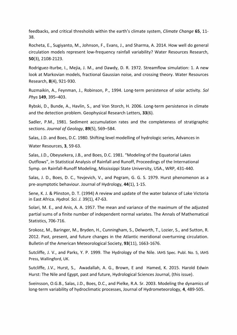
feedbacks, and critical thresholds within the earth’s climate system, Climate Change 65, 11-38.

Rocheta, E., Sugiyanto, M., Johnson, F., Evans, J., and Sharma, A. 2014. How well do general

circulation models represent low‐frequency rainfall variability? Water Resources Research,

50(3), 2108-2123.

Rodriguez‐Iturbe, I., Mejia, J. M., and Dawdy, D. R. 1972. Streamflow simulation: 1. A new

look at Markovian models, fractional Gaussian noise, and crossing theory. Water Resources

Research, 8(4), 921-930.

Ruzmaikin, A., Feynman, J., Robinson, P., 1994. Long-term persistence of solar activity. Sol

Phys 149, 395–403.

Rybski, D., Bunde, A., Havlin, S., and Von Storch, H. 2006. Long‐term persistence in climate

and the detection problem. Geophysical Research Letters, 33(6).

Sadler, P.M., 1981. Sediment accumulation rates and the completeness of stratigraphic

sections. Journal of Geology, 89(5), 569–584.

Salas, J.D. and Boes, D.C. 1980. Shifting level modelling of hydrologic series, Advances in

Water Resources, 3, 59-63.

Salas, J.D., Obeysekera, J.B., and Boes, D.C. 1981. “Modeling of the Equatorial Lakes

Outflows”, in Statistical Analysis of Rainfall and Runoff, Proceedings of the International

Symp. on Rainfall-Runoff Modeling, Mississippi State University, USA., WRP, 431-440.

Salas, J. D., Boes, D. C., Yevjevich, V., and Pegram, G. G. S. 1979. Hurst phenomenon as a

pre-asymptotic behaviour. Journal of Hydrology, 44(1), 1-15.

Sene, K. J. & Plinston, D. T. (1994) A review and update of the water balance of Lake Victoria in East Africa. Hydrol. Sci. J. 39(1), 47-63.

Solari, M. E., and Anis, A. A. 1957. The mean and variance of the maximum of the adjusted

partial sums of a finite number of independent normal variates. The Annals of Mathematical

Statistics, 706-716.

Srokosz, M., Baringer, M., Bryden, H., Cunningham, S., Delworth, T., Lozier, S., and Sutton, R.

2012. Past, present, and future changes in the Atlantic meridional overturning circulation.

Bulletin of the American Meteorological Society, 93(11), 1663-1676.

Sutcliffe, J. V., and Parks, Y. P. 1999. The Hydrology of the Nile. IAHS Spec. Publ. No. 5, IAHS

Press, Wallingford, UK.

Sutcliffe, J.V., Hurst, S., Awadallah, A. G., Brown, E and Hamed, K. 2015. Harold Edwin

Hurst: The Nile and Egypt, past and future, Hydrological Sciences Journal, (this issue).

Sveinsson, O.G.B., Salas, J.D., Boes, D.C., and Pielke, R.A. Sr. 2003. Modeling the dynamics of long-term variability of hydroclimatic processes, Journal of Hydrometeorology, 4, 489-505.

Todini, E., and O'Connell, P. E. 1979. Hydrological Simulation of Lake Nasser. Volume I.

Analysis and Results. IBM Italy Scientific Centres/Institute of Hydrology UK.

Tung, K.-K., and J. Zhou, 2013. Using data to attribute episodes of warming and cooling in

instrumental records. Proc. Natl. Acad. Sci. U.S.A., 110, 2058-2063.

U.S. Water Resources Council, 1981. Guidelines for Determining Flood Flow Frequency.

Bulletin 17B, US Department of the Interior.

Van Vliet, K. M., Van der Ziel, A., and Schmidt, R. R. 1980. Temperature‐fluctuation noise of

thin films supported by a substrate. Journal of Applied Physics, 51(6), 2947-2956.

Vogel, R. M.. Y. Tsai and J. F. Limbrunne, 1998. The regional persistence and variability of

annual streamflow in the United States. Water Resources Research, 34(12), 3445-3459.

Voss, R.F. and Clarke, J., 1975. “1/f noise” in music and speech. Nature 258, 317–318.

Voss, R. F., and Clarke, J. 1976. Flicker (1/f) noise: Equilibrium temperature and resistance

fluctuations. Physical Review B, 13(2), 556-573.

Wallis, J. R., and O'Connell, P. E. 1973. Firm reservoir yield—How reliable are historic

hydrological records?. Hydrological Sciences Journal, 18(3), 347-365.

Wang, C., and Zhang, L. 2013. Multidecadal ocean temperature and salinity variability in the

tropical North Atlantic: linking with the AMO, AMOC, and subtropical cell. Journal of

Climate, 26(16), 6137-6162.

Wu, Z., N. E. Huang, J. M. Wallace, B. V. Smoliak, and X. Chen, 2011. On the time varying

trend in global-mean surface temperature. Clim. Dyn., 37, 759–773.

Zhang, Y., Wallace, J. M., and Battisti, D. S. 1997. ENSO-like interdecadal variability: 1900-93.

Journal of Climate, 10(5), 1004-1020.

Zhou, J., and K.-K. Tung, 2012. Deducing multidecadal anthropogenic global warming trends

using multiple regression analysis. J. Atmos. Sci., 70, 3–8.

Zorita, E., T. F. Stocker, and H. von Storch, 2008. How unusual is the recent series of warm

years? Geophys. Res. Lett., 35, L24706.

Tables

Table 1 Definitions of Population Range and Adjusted Range

Denote a series of n random variables as , , …, with sample mean

and with E ( .

Population Range of cumulative departures:

= max ( ) – min ( )

Adjusted Range of cumulative departures:

= max ( ) – min ( )

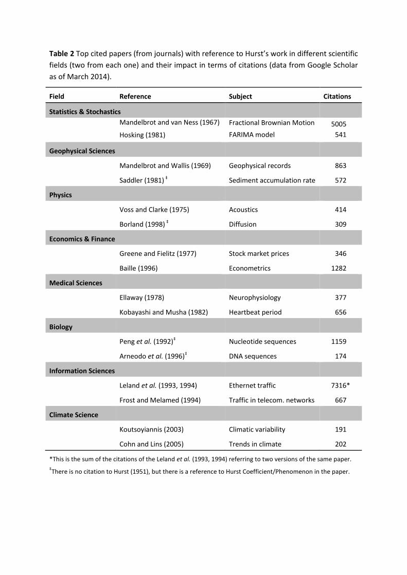
Table 2 Top cited papers (from journals) with reference to Hurst’s work in different scientific

fields (two from each one) and their impact in terms of citations (data from Google Scholar

as of March 2014).

Field Reference Subject Citations

Statistics & Stochastics

Mandelbrot and van Ness (1967)

Hosking (1981)

Fractional Brownian Motion

FARIMA model

5005

541

Geophysical Sciences

Mandelbrot and Wallis (1969)

Saddler (1981) ‡

Geophysical records

Sediment accumulation rate

863

572

Physics

Voss and Clarke (1975)

Borland (1998) ‡

Acoustics

Diffusion

414

309

Economics & Finance

Greene and Fielitz (1977)

Baille (1996)

Stock market prices

Econometrics

346

1282

Medical Sciences

Ellaway (1978)

Kobayashi and Musha (1982)

Neurophysiology

Heartbeat period

377

656

Biology

Peng et al. (1992)‡

Arneodo et al. (1996)‡

Nucleotide sequences

DNA sequences

1159

174

Information Sciences

Leland et al. (1993, 1994)

Frost and Melamed (1994)

Ethernet traffic

Traffic in telecom. networks

7316*

667

Climate Science

Koutsoyiannis (2003)

Cohn and Lins (2005)

Climatic variability

Trends in climate

191

202

*This is the sum of the citations of the Leland et al. (1993, 1994) referring to two versions of the same paper.

‡There is no citation to Hurst (1951), but there is a reference to Hurst Coefficient/Phenomenon in the paper.

Figures

Figure 1 The proliferation of Hurst’s work in different scientific fields.

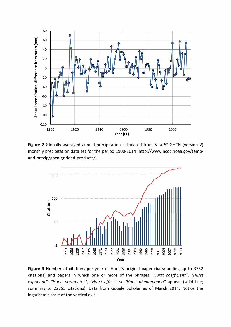
Figure 2 Globally averaged annual precipitation calculated from 5° × 5° GHCN (version 2)

monthly precipitation data set for the period 1900-2014 (http://www.ncdc.noaa.gov/temp-

and-precip/ghcn-gridded-products/).

Figure 3 Number of citations per year of Hurst’s original paper (bars; adding up to 3752

citations) and papers in which one or more of the phrases “Hurst coefficient”, “Hurst

exponent”, “Hurst parameter”, “Hurst effect” or “Hurst phenomenon” appear (solid line;

summing to 22755 citations). Data from Google Scholar as of March 2014. Notice the

logarithmic scale of the vertical axis.