the secret life of fear: interdependencies among implied ... · the secret life of fear:...
TRANSCRIPT

Graduate School Master of Science in
Finance Master Degree Project No.2010:130
Supervisor: Anders Johansson
The Secret Life of Fear: Interdependencies Among Implied Volatilities Represented by different Stock Volatility Indices
Treated as Assets
Saku Nousiainen

ii
ABSTRACT
Institution
University of Gothenburg, School of Business, Economics and Law, Graduate School
Study
Master’s Thesis
Title
The Secret Life of Fear: Interdependencies among implied volatilities represented by
different stock volatility indices treated as assets.
Pages
(6 +) 30 + 10
Author
Saku P. Nousiainen (Mr.)
Semester
Spring 2010
Degree Program
Master in Finance
Abstract
This study focuses on the systemic interdependencies of specified volatility indices, the underlying assets of
which are major stock indices of developed financial markets. The volatility indices in question follow the
standard VIX specification, and thus give forward-looking 30-day estimates of implied volatilities on each
market respectively. Volatility is then considered as an asset. Engle’s Dynamic Conditional Correlation
specification of the VAR-MVEGARCH -methodology is used to study spillovers in volatilities between
different markets, as well as dynamic conditional volatility and correlation structures. Additionally,
asymmetric behavior of volatilities is taken into account. The time period from January 2000 to mid-June
2009 includes both times of normal market conditions and crises. The results prove unidirectional spillovers
from the US VIX to other indices, and more locally from the VFTSE to the VSMI. The dynamic
conditional volatilities include abrupt and large short-term peaks, while the dynamic conditional correlations
(DCC) are high and stable. The deviations from DCC -means revert back smoothly so that the spillovers
between the indices take place over time, and can be interpreted as information transformation. The VDAX
and the VFTSE of the main European markets are highly unified, having high correlations but no spillovers
between them. All indices contain small but significant volatility asymmetries, and day effects.
Keywords
Dynamic Conditional Correlation, Implied Volatility, MGARCH, Risk Management, Time Series
Analysis, Volatility Index, Volatility Spillover
JEL Classification
C32, C53, G12, G13, G14, G15
Additional Information
This study is the 2010 winner of the Richard C. Malmsten Memorial Foundation Award for Best Master’s Thesis
in Finance at the University of Gothenburg Graduate Business School. The WinRats code written for the
modeling by the researcher is also available.

iii
PREFACE
Wonders of life… Volatility indices are absolutely one of them, revealing new things from the very beginning to the
very end, during the whole research process. And still, “I can’t conceive the nucleus of all, begins inside a tiny seed,
and what we think as insignificant, provides the purest” fear we feel!
I would like to thank everybody at HGU’s Finance community and Graduate School, as well as at the Centre for
Finance. First and foremost, my advisor professor Dr. Anders C. Johansson should be mentioned for his
encouragement and enthusiasm, I was privileged to get such a learning opportunity, and Dr. Joakim Westerlund for
sharing his indispensable knowledge in unit root testing in the existence of structural breaks. Thank you also to Dr.
Martin Holmen, whose flexibility and understanding, as the head of the Master of Finance program, helped me to
schedule reasonable timetables for my extensive travels in and out of Sweden. Furthermore, I would like to thank the
Wihuri Foundation for their financial support, which made this learning opportunity possible.
A special thank you goes to my newlywed wife Kristine, who had to adjust a lot to me living extensive periods in a
different country, and time to time on a different continent. She has persistently supported me through thick and
thin, even when I was willing to give in. Finally, as always, thanks to my Mom, Dad, and Johanna for never letting
me down.
Mr. Saku Nousiainen
Helsinki, May 12th, 2010

iv
LIST OF TABLES
Table 1: Available Volatility Index (VI) data for developed Stock Markets............................................................. 18 Table 2: Volatility Indices (VI) used in the study ....................................................................................................... 18 Table 3: Descriptive Statistics of the VI Returns........................................................................................................ 20 Table 4: Unconditional Correlations of Returns........................................................................................................ 20 Table 5: Engle-Ng (1993) Sign and Size Bias Test .................................................................................................... 21 Table 6: Univariate Akaike Information Criteria (AIC) ............................................................................................ 21 Table 7: Unit Root and Cointegration Tests............................................................................................................... 21 Table 8: Day Effects of the 1st Difference VI Returns ............................................................................................... 22 Table 9: Multivariate Information Criteria ................................................................................................................ 23 Table 10: VAR(1)-MVEGARCH Results ..................................................................................................................... 24 Table 11: Dynamic Conditional Volatilities (DCV)................................................................................................... 24 Table 12: Dynamic Conditional Correlations (DCC)................................................................................................ 25 Table 13: Residuals Diagnostics I............................................................................................................................... 26 Table 14: Residuals Diagnostics II ............................................................................................................................. 26

v
CONTENTS
1. INTRODUCTION ................................................................................................................................................1
2. LITERATURE REVIEW AND CONCEPTS..................................................................................................3
2.1. VOLATILITY AND IMPLIED VOLATILITY .............................................................................................................4 2.2. VOLATILITY INDICES (VI) ...................................................................................................................................5 2.3. VOLATILITY AS AN ASSET ...................................................................................................................................6
3. METHODOLOGY ...............................................................................................................................................7
3.1. RESEARCH QUESTIONS, HYPOTHESES AND ASSUMPTIONS .................................................................................7 3.2. RESEARCH SETTING .............................................................................................................................................8
3.2.1. Choice of time series and modeling ........................................................................................................9 3.2.2. Testing and residual based diagnostics ..................................................................................................9 3.2.3. Multivariate GARCH –modeling...........................................................................................................14
3.3. VALIDITY AND RELIABILITY OF THE METHOD...................................................................................................16
4. DATA....................................................................................................................................................................18
4.1. CHOICE OF DATA ...............................................................................................................................................18 4.2. PROPERTIES OF DATA.........................................................................................................................................19
5. RESULTS.............................................................................................................................................................23
6. DISCUSSION ......................................................................................................................................................27
6.1. ROBUSTNESS OF THE RESULTS...........................................................................................................................28 6.2. FURTHER RESEARCH..........................................................................................................................................29 6.3. CONCLUSIONS ....................................................................................................................................................30
REFERENCES............................................................................................................................................................31
APPENDICES .............................................................................................................................................................37
ENDNOTES.................................................................................................................................................................40

1
1. INTRODUCTION
This study continues the research tradition of interrelations between different financial markets – geographically
and/or asset wise – and the long and essential line of study of conditional volatilities of historical time series.
Volatility indices (VI), the data of the study, are by definition based on implied (i.e. forward-looking) volatilities of
derivatives written on underlying indices. Then, the study contains new and unique value by studying implied
volatilities of markets through volatility indices. More specifically, the historical time series of this study are VIs for
stock indices of the main developed markets in the Western world. Their systemic interdependencies are studied by
using a multivariate GARCH (MGARCH) –methodology, which has evolved a great deal recently. A new feature is
to treat VIs as assets, an approach not introduced earlier in this research setting as is.
Importance of the study. The study creates new bridges between theory and practice by studying properties and
interdependences in this new financial asset group in different markets (Ethridge 2004, 40; Ryan et al. 2002, 50).
These results can be utilized in many ways. A better understanding of VIs leads to insights into the use of indices as
market timing tools, measures of uncertainty of markets, and as proxies for stock variance swap levels (Carr & Wu
2006). From an asset management perspective, the results will uncover how beneficial it is to diversify inside the
volatility asset class, and reveals potential outcomes when a foreign VI is used to hedge investments in a traditional
asset class, such as stocks (Grant et al. 2007; Black 2006). Essentially, does investing in volatilities in different
markets bring any benefits, or is it enough to invest in volatility in only one developed market without any
aspirations for diversification? The question is meaningful right now: developed stock markets have been shown to
become increasingly correlated due to on-going international financial integration, but there are still few VIs available
(with derivatives written on them) for investing. Thus, investors may not have an opportunity to invest in volatility in
their own market, but a great deal of interest in investing in volatility in other developed markets. The time period
studied is interesting, as it includes the recent subprime crisis, the effects of which have been unprecedented on a
global scale. The study reveals how correlations change when extensive shocks take place in one of the markets.
By and large, the most important contributions serve volatility estimation (e.g. Satchell & Knight 2002), which is an
essential part of asset pricing. The increased understanding of volatilities of VIs, and information about their relative
relationships, is needed in pricing of derivatives written on these indices. This front is highly active with new VI
based derivatives created daily. Moreover, there are on-going attempts to advance existing pricing models for this
purpose (e.g. Sepp 2008; Soklakov 2008). Derivatives pricing treats VIs as assets, just as this study assumes.
Main findings. The study reveals that the behavior of VIs is highly correlated, and surprisingly stable, even during the
crises. The volatility process is persistent, and changes in dynamic conditional volatilities are extensive and abrupt, as
well as very short term. There exist unidirectional relationships between indices, the US VIX being the center and
main source of the shocks. The more remote Swiss VSMI is affected locally by the UK’s VFTSE. Spillovers are
interpreted as information transformation. The main European Union markets, the German VDAX and the UK’s
VFTSE are highly correlated, but without spillovers. The same applies to the German VDAX and the Swiss VSMI.
These findings show that proximity and closely related real economies seem to cause volatilities to evolve together,
while financial relationships seem to cause spillovers. Volatilities of implied volatilities represented by the indices
seem to all have a small but consistent asymmetric element. The distributions of the 1st difference returns are non-
normally distributed. The time series also contain day effects.

2
Structure of the report. The study is reported by loosely following the standard Introduction – Methodology – Results –
Discussion (IMRD) –format (Hirsjärvi, Remes & Sajavaara 1997, 232-250). The literature review is separated from the
introduction, as well as the methodology from the data chapter. The validity and reliability of the method, and the
robustness of the results, are studied separately.

3
2. LITERATURE REVIEW AND CONCEPTS
Volatility index (VI) related research. Much of the research on VIs has focused on explaining the use of the VIX index –
and later derivatives written on it – in applied use, and is needed as such only as a basis for correct data treatment
and soundness of the research framework. Probably the most important contribution in the field of VIs thus far is
that of Carr & Wu (2006). They explain the mathematical and economic properties, motivate the redefinition of VIX index
in 2003, and show how the index is related to the volatility and option theory, as well to variance swaps.
Furthermore, they look at historical behavior of the index, and pay attention to the leverage effect, which has been
given multiple explanations in related literature (Bekaert & Wu 2000; Black 1976; Campbell & Hentschel 1992;
Campbell & Kyle 1993; Haugen et al. 1991). They also find “potential discontinuous index return volatility
movements”, relate it to the findings of Eraker, Johannes & Polson (2003), and together with Wu (2005) notice that
the variance rate contains a significant jump component, the arrival rate of which is not constant but proportional (also
Becker, Clements & McClellant 2009). Carr & Wu (2006) show that the forward-looking VIX as an implicit volatility
proxy is alone enough to estimate the volatility of the underlying index, when compared to a historic estimate of
GARCH(1,1), which Ahoniemi (2008) finds suitable as a different historic estimation model. There are several
sources (e.g. Banerjee, Doran & Peterson 2006; Cipollini & Manzini 2007), which claim that the implied volatility of
the VIX can predict the future returns of its underlying index, but numerous sources disagree (Becker, Clements &
White 2007; Hsu & Murray 2007). Majmudar & Banerjee (2004) notice that the EGARCH -model is best suited for
VIX modeling, among the other GARCH specifications.
Black (2006) presents a positive skew and kurtosis of probability distributions, and pays attention to the mean-
reversion property. Gonzalez-Perez & Guerrero (2009) state that the properties of the VIX index are exceptional
including non-normality, heteroscedasticity, non-linearity, and most importantly, non-stationarity. They recognize
that non-stationarity is not always assumed in research, and consequently, this opinion cannot yet to be considered as
a final view of the research community. Moran & Dash (2007; also Siriopoulos & Fassas 2008; Cipollini & Manzini
2007) indicate some properties for (spot) VIs, such as high volatility and negative, but asymmetric, correlation with the
respective underlying market indices. They also indicate mean-reversion and state that VIs can be used as a) an
indicator of market fear (also Whaley 2000, 2009i), b) in hedging (through derivatives)ii. Grant, Gregory & Lui
(2007), as well as Szado (2009), introduce VIs as c) an asset class. Lately, Whaley (2009) has defined the historical
development of the VIX, and described its position in the wider framework of market indicators. Jiang & Tian
(2007) maintain that even the current definition of the VIX index might be flawed. This proposition disagrees with
most earlier findings.
Volatility co-movements and spillovers. Aboura (2003) conducts the only implied volatility (Day & Lewis 1988, Canina &
Figlewski 1993, Christensen & Prabhala 1998) transmission study to date (to the researcher’s knowledge) by using
VIs (VX1, VDAX & VIX). He finds implicit processes especially using the mean-reverting jump model and
GARCH-GJR –specifications and, advancing the findings of Erb et al. (1994) and Longin & Solnik (1995), maintains
that correlations depend on implied volatility and business cycles, and change because of different skew and kurtosis
in the true return time series. These differences function as a source for correlation asymmetry (Aboura 2003, 15-16).
Earlier research has approached the topic mainly by modeling return and historical variance, most often by using
different GARCH -applications (Andrews 1991, Satchell & Knight 2002). This line of research can be divided into
sub-sections, studies which research co-movements of returns (e.g. Copeland & Copeland 1998; Andersen &
Bollerslev 1997; Susmel & Engle 1994), and those more interested in volatility co-movements. The latter group
included Ross (1989), who proved that co-movement studies of volatility are meaningful. Schwert, French &

4
Stambaugh (1987) noticed volatility persistency and introduced the volatility feedback effect. Theodossiou & Lee (1993)
found weak volatility overflows, and that conditional volatility in many markets originated in the USA. They also
found strong own-volatility spillovers over time. Koutmos & Booth (1995), as well as Booth et al. (1997), studied
asymmetric volatility spillovers by using a Multivariate EGARCH concept, and noticed that bad news seemed to
have greater effects than positive. There are also a number of studies showing that trading has an essential
connection to (especially intra-day) volatility. Some sources do not accept volatility spillovers at all, but consider
them as a result of non-synchronous trading (Lin et al. 1994), while the majority (e.g. Stoll & Whaley 1990; Chan,
Chan & Karolyi 1991) interprets them as information transmission.
Day of the week effects. There is lots of international evidence that equity, fixed income, derivatives (Gay & Kim 1987)
and foreign exchange markets contain seasonal, monthly or weekly anomalies. Osborne (1962), Cross (1973) and
French (1980) analyze the so-called Monday effect, which according to Lakonishok & Levi (1982), could be caused
by the behavior of market transaction systems. Keim & Stambaugh (1984) speak about the weekend effect, caused
by measurement errors in stock prices. Further studies focus on separating the effect of trading and non-trading
periods (Rogalski 1984), focus closer on the properties of the effects (Chang et al. 1993), explain roles of informed
and liquidity traders (Foster & Viswanathan 1990), as well as interday effects (Foster & Viswanathan 1993). There is
some later evidence that the effect has disappeared from some markets. The studies are most often undertaken by
using different sorts of OLS and GARCH–specifications (Engle 1982; Kiymaz & Berument 2003; Apolinario &
Caro 2006).
2.1. Volatility and Implied Volatility
Volatility of assets is generally considered important in financial modeling, as it has a large effect on asset prices. Hull
(2009, 285) defines volatility as a sign of the arrival of new information on the market, but reminds us that volatility
is partially caused by trading itself. Volatility is often seen as an outcome of volatility drivers such as inflation, oil and
other commodity prices, as summarized by Zimmermann et al. (2003, 121-126). According to them, a special class of
volatility drivers is created by currency, interest and market, which function also as value drivers (Fama 1965; French
1980; French & Roll 1986). Hence, there are lots of studies focusing on volatility estimation, the most important
results of which can be found as secondary sources (e.g. Satchell & Knight 2002). One common property of
volatility is mean reversion (Hull 2009, 482-483), and as the standard GARCH –models follow a mean reverting
stochastic process (Engle 1982), they are practical for volatility modeling in practice. Mean reversion can be masked
by the fact that the volatility time series may contain structural breaks and jumps. These problems are sometimes
taken into account by using jump-diffusion models (Merton 1976) or stochastic volatility models (Hull & White
1987; 1988; Gatheral 2006; Sheppard 2005).
Implied volatility refers to future looking volatility estimated from derivatives markets by using derivatives pricing
models such as Black & Scholes (1973; Black 1989; Merton 1973) – most often based on risk-neutral valuation
methods (Smith 1976). This is possible, as market prices (and all other variables) for derivatives are known (Hull
2009, 296). Both Carr & Wu (2006), Ahoniemi (2008) and Graham & Harvey (2009) have shown that there are clear
relationships between the implied volatility of VIs, and the historical time series based volatility estimations. Still,
Siriopoulos & Fassas (2008) claim that the VFTSE index contains information beyond historical volatility.

5
2.2. Volatility Indices (VI)
History and definition. VIs first saw the light as private tools for derivatives traders, the specifications of which used to
differ. Soon, they spread among a large audience, and became a standard measure of risk for stock indices (Whaley
2009). The indices chosen for this study are all constructed using an improved VIX -specification, which has become
the first globally accepted standard specification for VIs. The general formula for VIX, defined in the so-called White
–paper (CBOE 2009; also Carr & Wu 2006, 14; Whaley 2009), is a “kernel-smoothed estimator” and can be presented
as
!
VIXt=
2
T
"Ki
Ki
2eRTOtK
i( ) #1
T
Ft
K0
#1$
% &
'
( )
i
*2
+100 (2.1)
at time t , where T is time to expiry for options included specified on the minute level of preciseness, and
!
Ft is a
forward index level derived from index options. If the first strike below this forward index level is,
!
K0, the strike
price for the out-of-the-money option, i , is presented by
!
Ki, which is call, put or both call and put options by
following
!
Ki
> K0: Call
< K0: Put
= K0: Both
"
# $
% $
. (2.2)
The interval between strike prices,
!
"Ki, is calculated by
!
"Ki=K
i+1 #Ki#1
2, (2.3)
the continuously compounded risk-free rate is R , and the middle point in the bid-ask spread for each option with
!
Ki, is presented by
!
OtK
i( ) . Lately, new VIs have been introduced both in the new markets, in India, Hong Kong,
and Japan, as well as for new underlying indices such as commodities.
Properties of volatility index (VI). A VI, defined by this specification, gauges a measure of the 30-day implied volatilities
of the entire volatility smile [sic], is quoted in percentage points, and according to Szado (2009, 9-10) cannot be
modeled by using cost of carry model. A common, and heuristically understandable, property of volatility is mean
reversion, as the uncertainty measured by volatility cannot increase eternally. There is a general understanding that
VIs are mean reverting and thus stationary (Black 2006; Moran & Dash 2007). In practice, VI series may contain
jumps and structural breaks, which make confirming this property less clear-cut (Aboura 2003). The improved VIX -
specification is considered sound by many sources (Carr & Wu 2006), which is confirmed by the fact that the
squared VI value can be considered as the variance swap rate on the underlying index (Carr & Wu 2006, 19-20). Still,
Jiang & Tian (2007) have suggested that the VIX –specification may underestimate by 198 or overestimate by 79
basis points the volatility of an underlying asset. These questions still remain open. In terms of other properties, Carr
& Wu (2006, 18-19) have revealed that at least the VIX index is affected by the leverage effect, the reasons of which
can be numerous (more closely Bekaert & Wu 2000; Black 1976; Campbell & Hentschel 1992; Campbell & Kyle
1993; Haugen et al. 1991; Hull 2009, 395) and contains The Federal Open Market Committee Meeting Day effect, which

6
increases the values of the index roughly 4 trading days before the meeting (ibid, 19-21). Other VI related day effects
have not been reported earlier.
Applications. VIs have useful properties that can be utilized for a variety of purposes. They are used 1) to measure
uncertainty, as they estimate implied volatilities for the future, and serves then as a practical measure for “fear”
(Whaley 2000, Moran & Dash 2007) in the Finance industry. It is also 2) a natural tool for market timing, as it reveals
volatility peaks time-wise, by being negatively correlated with stock markets (Black 2006, 12), or 3) to improve skew
and kurtosis properties of other investment through derivatives (ibid., 12). In this sense, VIs create a new asset class,
as they allow diversifying investments in the implied volatilities (Grant et al. 2007; Szado, 2009). Further, 4) VIs
reflect the variance swap levels of their underlying index (Carr & Wu 2006, 19-20). Hence, increased knowledge of
these indices, serves not only the highly important front of volatility estimation, but can be utilized in wide variety of
purposes from asset allocation and market timing to variance swap pricing and interdependency of markets.
2.3. Volatility as an Asset
One fundamental assumption that has a large impact on the results and reliability of the study is to treat volatility as
an asset (Grant et al. 2007). This is a natural direction of development in applied studies (e.g. Black 2006; Szado
2009), as the markets are further and further securitized, and the VIs are based on the prices of derivatives, which are
assets themselves. However, considering risk as a separate asset class along with stocks, bonds and commodities is
recent and useful in serving asset management and derivatives pricing (e.g. Sepp 2008; Soklakov 2008). It also helps
to mitigate potential data-related problems.
There are numerous factors that might bring uncertainty to the data. The VIs might be calculated by using different
specifications, or for different time lengths. The number of options and their available maturities, the implied
volatilities of which are used to calculate the index, might differ. Additionally, the ways these options are used might
differ from market to market, for example, if competing products are readily available in one market for investors to
use. Further, the underlying stock indices are fundamentally different from each other. Stock indices consist of a
varying number of companies, the types and relative weights of which may be chosen using different criteria –
sometimes the index contains only the most actively traded stock series of a company. Efficiency in the markets may
differ to a degree, as well as trading and transaction costs. The treatment of volatility as an asset is a clear-cut detour
around these problems. When VIs are considered simply as market value of an asset for the risk of the underlying
stock index, these market values can be measured as is without the need to evaluate the afore-mentioned problems in
the data.iii Finally, treating volatility as an asset, affects the definition of implied volatility. The VI should not be seen
as an unbiased measure of volatility anymore, but as an asset, the price of which implicitly refers to the implied
volatility of underlying index and the related market.

7
3. METHODOLOGY
The rationale of the study is to advance volatility spillover research by observing the systemic behavior of implied
volatilities as expressed by VIs. This paper analyzes the implied volatility spillovers between different markets (mean
equation) and dynamic conditional volatilities and correlations (variance equation) between these volatility assets in
the international context. In other words, the study continues traditional research of volatility and market integration
by using a contemporary systemic point of view, and expands newer, more applied research approach, which treats
volatility as an asset. This latter approach has become meaningful because of the on-going securitization process of
financial markets. There is no generally accepted conceptual framework or methodology (Ethridge 2004, 148) for the
study, as the research topic is relatively new.
3.1. Research questions, hypotheses and assumptions
The research questions. The objectives of the study are defined on two levels – as a general perspective, and by
narrowing this perspective to specific problems. The research problems are then defined as a general question, which
is studied through practical sub-questions (Ethridge 2004, 87). The general objective of the study is to examine:
QG: What kinds of relationships between stock volatility indices of different developed and discrete
markets can be observed, when these indices are treated as assets?
This objective is answered through more applied sub-questions:
Q1: Are there implied volatility spillovers between the volatility indices in question?
Q2: How do volatilities and correlations change over time, and what kind of variance-covariance
matrix they create?
Q3: Are there asymmetric volatility effects?
The most reasonable approach to answer the sub-questions is to use a Multivariate GARCH- methodology, which
allows studying of spillovers between VIs (Q1), by including a mean equation in the Vector Autoregressive fashion,
and which also generates a covariance (or correlation) matrix describing relationships between the implied volatilities
represented by the indices (Q2). The Dynamic Conditional Correlations (DCC) specification (Engle 2002) takes into
account a possibility that volatilities and correlations are changing dynamically over time (Q2), and is capable of
describing these changes. The time window includes both times of ordinary market behavior and the latest subprime
crisis. The distributions of VIs are often non-normal, and the volatilities of VIs, just like volatilities of different
assets, are not always normal and symmetric (Carr & Wu 2006; 18-19) – a phenomenon not thoroughly understood
yet. Potential asymmetry is taken into account by using the appropriate EGARCH -specification (Q3). Answering
these questions gives new insights about the interdependencies of VIs. As the underlying indices are the main stock
indices of discrete developed Western markets, the findings also speak about spillovers, contagion and correlations
of uncertainty on the market level (QG).

8
Hypotheses. The case study setup studies the behavior of the markets in history. Hypotheses are not needed, and pre-
set views might lead to faulty analyses (Ethridge 2004, 144). Instead, the main focus lies in describing and illustrating
the findings.
The underlying assumptions behind the research questions. By continuing earlier research and following a specified
methodology, the study relies on several assumptions. The most essential are assumptions of:
a) Engle’s DCC-MGARCH –methodology and assumptions related to it (Engle 2002, 342).
b) The time series of the VIs in question are mean reverting (Ahoniemi 2008; Black 2006, Moran & Dash
2007; Szado 2009,12), and
c) their implied volatility values, created by using the VIX- specification and derivatives on the main market
indices, can be considered as sound market prices of risk for the underlying stock indices (Carr & Wu
2006). Still, the fact that investing in VIs takes place through derivatives is not taken into account (Black
2006).
d) The traditional assumptions of financial markets: rational agents, competitive markets, freely available
information and no arbitrage, (Ryan et al. 2002, 51-53, see also Hull 2009, 286-287, 289) are implicitly
important, as VIs are based on the prices of derivatives. Still, the new VIX specification is free from pricing
models used [sic].
e) Finally, for practical conclusions about the relationships of markets, an assumption can be made that a VI
has an ability to portray implied volatility of the overall stock market in question, as the VI is based on the
respective main stock index.
3.2. Research setting
By following Ethridge the study can be classified as representative of analytical applied research (2004, 20-25), or by
following Johnson (1986, 12-13) as disciplinary problem-solving or subject-matter research (Mäki, Gustafsson,
Knudsen 1993, 121-128), as the study represents the realm of one single domain. Measured by Laughlin’s
classification of theorization (Ryan et al. 2002, 44-46), the article represents a high or medium class of prior theory,
and a high level of methodological choice.
Preliminary Research. The pre-research of the data is undertaken as suggested by Gaines (2002). It reveals that many
VIs seem to contain a unit root, when traditional unit root tests (KPSS, Augmented Dickey-Fuller, and DF-
Generalized Least Squares) are used. This is an interesting finding, as volatility should have a theoretical tendency to
be mean reverted (Moran & Dash 2007, 98). As stated earlier, there are several potential explanations for this based
on general volatility research. Earlier VI related studies explain this phenomenon often as an occurrence of structural
break(s), and treat the time series as stable even if the data fulfill this property weakly (Ahoniemi 2008; Black 2006).
However, special attention is paid on unit root testing in the study.
General process. The research process is described in appendix 1, which explicitly shows the theoretical and applied
segments of the research process. The theoretical framework is created through 2) methodological decisions of the
study, which are in turn founded in 1) earlier research. The applied research process begins by 3) choosing
appropriate data and studying its statistical properties. All the tests are run for the data both as logarithm and first
difference values (equation 3.1). Potential day effects of the data are studied, in order to decide whether the use of
daily or weekly data would yield more reliable results, and the final choice of the 4 VI series included in the model
are made. 4) The most suitable MGARCH –model is then chosen for estimations by relying on residual based
diagnostics, summary statistics and information criteria. Hence, these two steps (3-4), as well as methodological
orientation (2), create a cyclical, repeated process in practice. 5) The results of this applied process are then reported

9
and discussed, and the robustness of the results is evaluated. In this context, it is also natural to evaluate the meaning
of the findings with respect to theoretical framework, as well as a basis for future study. Still, generalization of the
results of the applied study has several limitations and should be handled with care.
3.2.1. Choice of time series and modeling
On one hand, the indices for modeling are chosen (among available ones) to portray differences between different
developed markets. On the other hand, this choice is also affected by modeling. The overlapping indices in terms of
geographic areas, fiscal and monetary policies are avoided, as well as the same currency. The study treats implied
volatility as a tradable asset, which means that the specifications of the indices could vary without jeopardizing the
research setting. The estimated models are complex, and the models do not necessarily converge. The process is
repetitive, as the number of time series in one model is limited by its convergence. These limitations are also
dependent on the properties of each time series and can change case by case.
3.2.2. Testing and residual based diagnostics
General Portmanteau tests are used to reveal possible deviations of data from randomness. Tests of autocorrelation,
heteroscedasticity, but also specific tests for volatility, namely tests for ARCH effects and asymmetric volatility are
executed three times, 1) for the daily data series in order to choose the appropriate model for the day effect testing,
2) for the weekly data series in order to choose the appropriate MGARCH model, and finally 3) as a residual based
diagnostics (Bauwens et al. 2006) for the error terms of the MGARCH model, in order to give further information
of the appropriateness of the model. The residual based diagnostics is conducted by following Johansson &
Ljungwall (2009), who study MGARCH error terms as separate univariate time series without combined testing
(ibid., 101-102). The residual based diagnostics are not a reliable verification tool by themselves, as their distributions
for daily and weekly time series may not followed assumed distribution (ibid., 96, 102). As a consequence, ARCH
effects are used to bring extra information in addition to LB tests. Information criteria are used where appropriate
numbers of lags for the time series are needed.
Summary statistics. The basic properties of the data such as the number of observations, mean, standard deviation,
minimum and maximum values, skew, excess kurtosis, Jarque-Bera measureiv and unconditional raw correlations are
reported as natural logarithms and as raw returns calculated by
!
"yt =100* lnyt
yt#1
$
% &
'
( ) . (3.1)
The 1st difference returns reported in the study are consistently calculated by using the specification in equation (3.1).
The used methodology may allow an opportunity to conduct the research by using natural logarithms along the
differences of the natural logarithms (e.g. Ahoniemi 2008). In modeling, the previous benefits from containing more
information, while the latter has an advantage of being more likely to converge to a solution. The graphical
presentations of the time series are also included.
Testing for day effects. The choice between daily and weekly frequency of data must be made. In practice, weekly data is
given a priority in order to avoid problems caused by potential non-synchronous trading (chapter 4.1). The use of
weekly data may mask the spillovers, however, and it is reasonable to verify the results by using daily values. Hence,
day effects are also studied for reference. The standard Ordinary Least Squares (OLS) -method is used

10
!
yt ="0
+"1D1+"
2D2
+"3D3
+"4D4
+ # (3.2)
where
!
" s are coefficients, y is the return of the data series at time t, Ds are are dummies for weekdays from Monday
to Thursday. Newey-West’s heteroskedasticity-and-autocorrelation-consistent (HAC) standard errors (Newey &
West 1987; also e.g. Verbeek 2008, 118-119) are used to mitigate potential autocorrelation and heteroscedasticity of
the time series (Gonzalez-Perez & Guerrero 2009, 2). Newey & West establish HAC errors by creating a general case
of Eicker’s (1967, according to Verbeek 2008, 94) heteroscedasticity-consistent covariance matrix, the positive
(semi)definiteness is confirmed by using Bartlett weights, as an alternative to GLS –method. The lags are defined by
information criteria. Eicker-White’s robust error terms (e.g. Verbeek 2008, 94-95), as well as EGARCH –results
(Nelson 1991; also e.g. Brooks 2008, 406), including the dummies in the mean equation, are estimated for reference.
Tests of autocorrelation, heteroscedasticity, and ARCH effects. Ljung-Box (LB) test (1978) is used to detect autocorrelation
and heteroscedasticity, mainly because it can catch also higher order autocorrelation and has better small sample
properties than Box-Pierce equivalent. In the Ljung – Box test statistic
!
LB = T T + 2( )ˆ " k
2
T # k~ $ 2
(m)k=1
m
% where
!
ˆ " k
=#k
#0
(3.3)
and T refers to sample size, m to maximal lag length and k those lag lengths from 1 to m. The distribution of the test
follows Chi-squared asymptotically. Tau- values are derived from standard autocovariance function
!
" k = E yt # E yt( )( ) yt#k # E yt#k( )( ) (3.4)
where y refers to values of the return data series at time t or univariate error terms of VAR-MVEGARCH model.
The asymptotic properties of Ljung-Box test are known only for the residuals of ARMA –type regressions. This
means that the diagnostics for MGARCH residuals cannot be given any formal asymptotic distribution, and thus
must be handled with care. In the beginning, the test is applied to the raw returns time series themselves, as the
results are the same as they were for the error terms of the regression including only a constant. This is a common
and generally accepted practice. The joint tests are run in 4 groups for lags 1-4, 5-8, 9-12 and 13-16. For each of the
group, Null-hypothesis assumes that all 4 taus are equal to zero, as
!
H0: "
1= 0,"
2= 0,"
3= 0,"
4= 0 or (3.5)
!
H1: " k # 0(any) , where
The alternative-hypothesis is true. Heteroscedasticity is tested the same way by using y2 terms in the beginning, and
MGARCH error terms for the residual diagnostics.
Engle’s (1982) classic methodology is used to test ARCH effects in the time series, in order to see whether GARCH
-type model specification is needed for the data. The ARCH effects are tested by
!
ˆ y t2
= "0
+ " lˆ y t# l
2+$
l=1
q
% and
!
TR2~ " 2(q) (3.6)

11
where
!
" are coefficients,
!
" is an error term, and q is a maximum number of explaining lags, l. The variable y is
defined as earlier. The test relies on R2 -statistics of the regression, which multiplied by sample size, T, asymptotically
follows Chi-squared distribution, with q degrees of freedom. The joint testing of
!
" s, and consequent Null- and
Alternative hypotheses are constructed as in equation (3.5). The test is also run on squared values, just as the LB test,
and used as a residual diagnostics for error terms as well. The test is theoretically most founded when used for error
terms of ARMA-model, but Brooks (2008, 389) maintains that the test can also be run on the raw returns data. The
researcher’s own findings reveal that there are infinitely small changes in the results and the statistical significance,
when using raw data.
Asymmetries in volatility. The potential need for asymmetric GARCH-models is tested, by using the sign and size bias test
of Engle & Ng (1993). The test relies on studying the error terms of the GARCH -model used. The standard
symmetric GARCH(1,1) model (e.g. Brooks 2008, 392-395)
!
yt = µ + ut where
!
ut~ N 0,"
t
2( ) (3.7)
!
"t
2=#
0+#
1ut$1
2+ %"
t$1
2
(3.8)
is estimated. The terms of the model are mean,
!
µ, return y of the data series at time t, and conditional volatility,
!
" 2,
at time t, and lagged and squared error terms of the mean equation, u, which are normally distributed with zero
mean.
!
" s and
!
" are non-negative coefficients. The model generates the error terms for the OLS -based asymmetry
test procedure. Later, VAR-MVEGARCH -model (equation 3.21-3.29) is used for the same purpose, when running
for residual diagnostics. Only the joint Engle-Ng -test is run on the error terms as
!
ˆ u t
2= "
0+ "
1S
t#1
#+ "
2S
t#1
#u
t#1+ "
1S
t#1
+u
t#1+ $
t and
!
TR2~ " 2(3) , (3.9)
which includes these before-mentioned error terms, u, coefficients,
!
" , dummies for negative and positive error
terms, S- and S+, as well as a new error term for the regression,
!
" . Then, the coefficient
!
" 1 signifies sign bias, where
the sign of the shock affects the future volatility the differently, while
!
" 2 and
!
" 3 reveal size bias, which means that
also magnitudes of the shocks have differing impacts. The test statistics follow asymptotically Chi-squared
distribution with 3 degrees of freedom, and is calculated as earlier. The joint Null -hypothesis indicates no
asymmetric effects.
Unit Root Tests. The unit root tests are used to reveal potential diversions of the time series from stability. Potential
unit roots should be taken into account when constructing the mean equation (3.21) of VAR-MVEGARCH -model. In
addition to standard Augmented Dickey-Fuller (ADF) test (e.g. Verbeek 2008, 286-288; Brooks 2008, 329-332), also
Zivot & Andrews (1992) and Lee & Strazicich (2004) tests are included to trace a potential structural break (see also
Westerlund 2009; Westerlund & Edgerton 2007), which might be caused by the subprime crisis period included in
the time series, and to take into account a possibility that the VIs would contain unit roots (Gonzalez-Perez &
Guerrero 2009). Zivot & Andrews (1992) test is well-known and advances Perron’s adjusted ADF -testing strategy,
by defining the crash model (A), for changes in the intercept,
!
yt = ˆ µ A + ˆ " A DUtˆ # ( ) + ˆ $ A t + ˆ % A yt&1
+ ˆ c jA'yt& j
j=1
k
( + ˆ ) t , (3.10)

12
and the combined model (C), for changes in both intercept and trend,
!
yt = ˆ µ C + ˆ " C DUtˆ # ( ) + ˆ $ C t + ˆ % C DTt
* ˆ # ( ) + ˆ & C yt'1+ ˆ c j
C(yt' j
j=1
k
) + ˆ * t (3.11)
where the difference raises from the
!
Tt
*, which is the time of exogenous break in the trend function. In both
models, the circumflexes refer to estimated parameters,
!
ˆ µ is constant, D refers to dummy variables, k –number of
parameters
!
"yt# j are to ”eliminate possible nuisance-parameter dependencies in the limit distributions of the test
statistics caused by temporal dependencies in the disturbances” (ibid.), and
!
ˆ " refers to the break in the data series.
Then,
!
DUt "( ) =1 if t # T"
0 if else
$ % &
and (3.12)
!
DTt* "( ) =
t #T" if t $ T"
0 if else
% & ' (3.13)
The unit root is then tested by rejecting Null-hypothesis if
!
inf"#$
tˆ % i"( ) <&
inf,%
i where i= A, C (3.14)
and in which
!
"inf,#
i is the left-tail critical value
!
" of t-statistics for
!
" i=1, from the asymptotic distribution of
!
inf"#$
tˆ % i"( ) , the distribution and the test statistics of which Zivot & Andrews establish in their paper (ibid.)
with
!
" = 0.001, 0.999[ ] . As is the case with Lee-Strazicich test, the drift only specification exists also for Zivot-
Andrews, but is seldom needed in practice (Lee & Strazicich 2004, 3).
Lee & Strazicich (2004) draw attention to some problems with Zivot-Andrews test, which they classify as
”endogenous break unit root test” (p. 1). The test results, according to them, might incorrectly conclude that ”a time
series is stationary with break when in fact the series is non-stationary with break. As such, ’spurious rejections’
might occur and more so as the magnitude of the break increases.” They suggest a new minimum Lagrange
Multiplier (LM) unit root test to avoid this problem. The concept (ibid.) is a modification of Schmidt-Phillips non-
break Unit Root test, the data generating process of which
!
yt = "'Zt + Xt where
!
Xt= "X
t#1 + $t (3.15)
follows Schmidt & Phillips (1992) – where Null-hypothesis of a unit root is
!
"=1 and vector
!
Zt= [1, t]’.
Lee & Strazicich’s complex contribution is to define a crash model (for changes in the intercept) with
!
Zt
= 1,t,Dt[ ]' where
!
Dt =1 if t " TB +1
0 if else
# $ % (3.16)

13
and
!
TB
is the time of the structural breakv, as well as a combined model (for changes in both intercept and trend) with
!
Zt= 1,t,D
t,DT
t[ ]' where
!
Dt =t "TB if t # TB +1
0 if else
$ % & (3.17)
similarly. Vector of coefficients,
!
"', is to be increased accordingly. Then, the test statistics is generated by regression
!
"yt = #'"Zt + $ ˜ S t%1+ ut
where
!
˜ S t = yt " ˜ # x " Zt˜ $ (3.18)
and in which
!
" = 0 is the Null-hypothesis,
!
˜ " refers to the coefficients in the main regression, and
!
˜ " x refers to the
restricted Maximum Likelihood Estimator of
!
"x#" + X
0. (3.19)
There are two things to notice. First, differencing removes the first value (t=1), and that the test statistics regression
(3.18) needs
!
"Zt instead of
!
Zt, which then become
!
"Zt= 1,"D
t[ ]' and
!
"Zt= 1,"D
t,"DT
t[ ]' (3.20)
for the crash model and the combined model respectively. Hence,
!
"Dt refers to a change in intercept and
!
"DTt to
trend under Alternative hypothesis, as well as a one time crash and a permanent change in the drift under Null-
hypothesis. The drift only specification exists, but is seldom needed in practice (ibid.). The autocorrelated errors can
be corrected by including augmented terms as in the basic Augmented Dickey Fuller test (e.g. Verbeek 2008, 286-
288; Brooks 2008, 329-332). The location of the break point is not needed for the study and thus not explicitly
specified. Lee & Strazicich (2004) also compare the results of their test with Zivot-Andrews test. They conclude the
LM test truly removes the problem by estimating the break point correctly and by being free from size distortions
and spurious rejections in the presence of the unit root.vi The possibility of multiple structural breaks is also studied
by following Lee & Strazicich (2003).
Testing for Cointegration. The failure in rejecting the unit roots in the time series means that the 1st differences of the
time series must be used. Further, Vector Error Correction Model (VECM) –parameters (e.g. Verbeek 2008, 340-
341) should be included in the mean equation of the MGARCH –model, if the time series were cointegrated. The
cointegration of the simultaneous time series is studied by following normal Johansen methodology (Brooks 2008,
350-355), in which Null -hypothesis suggests that there are r cointegrating relationships. If the hypothesis is rejected,
the new Null –hypothesis tests for r + 1 cointegrated equations. The procedure is repeated until the maximum rank
of cointegrations is found.
Choice of lags in the tests and models. The number of time lags must be chosen both for the used tests and for the main
model. These decisions are made a) by using predefined number lags (4, 8, 12, 16) for joint testing and reporting all
the results, as in Portmanteau tests, or b) by using standard univariate Akaike information criteria (AIC) as in the
study of day effects and unit roots. The choice of appropriate number of mean equation lags for MGARCH –model
is based on c) the multivariate versions of Akaike, Schwartz’s Bayesian (BIC), and Hannan-Quinn (HQIC) –
information criteria (e.g. Verbeek 2008, 61-64, 299-302; Brooks 2008, 232-239, 294-295). The final decisions are

14
made based on information criteria and residual based diagnostics of VAR-MVEGARCH –model together, in order
to compensate known weaknesses in the use of either of them. The Johansen cointegration test uses always the same
number of lags as the MGARCH –model used.
3.2.3. Multivariate GARCH –modeling
The main modeling endeavor is undertaken by using the Multivariate version of the Generalized Autoregressive
Conditional Heteroscedasticity (MGARCH) Maximum Likelihood estimator. The time series including volatility
clustering are traditionally modeled by using GARCH (Engle 2001, Gourieroux & Jasiak 2001, 126-135), and it has
become a standard method of analyzing a financial time series including time-varying volatilities (Engle 1982, 2001;
Engle & Bollerslev 1986). The model has different variations, and the EGARCH version has been successfully used
to model asymmetric behavior of volatility in the earlier stock market study.
The first generation MGARCH models have weaknesses, which make them difficult to use in practice. The simple
definition of MGARCH consisting solely of univariate specifications (without correlation part) is barely believable,
whereas Bollerslev, Engle & Wooldridge’s (1988) VECH –specification has a large number of parameters, is often
unable to yield a positively definite variance-covariance matrix, and it can be only used to estimate a few time series
at the time. BEKK –specification (Engle & Kroner 1995), on the other hand, decreases the number of parameters,
by assuming a positive definiteness of the variance matrix. Still, it does not converge very well, especially when a
larger number of time series is included, and it is difficult to include asymmetry in the model. Hence, second
generation models, which are estimated in two steps (Bauwens et al. 2006, 98-99), are more appropriate for practical
applications. Silvennoinen & Teräsvirta (2009, 223) also show that more advanced models have an overall tendency
to be more reliable.
Engle’s version of the Dynamic Conditional Correlation (DCC) model used for estimation (Engle 2002; about
different specifications Bauwens et al. 2006, 91) is successfully used by Silvennoinen & Teräsvirta (2009) in the VIX
context without convergence problems. The Vector Autoregressive Multivariate Exponential Generalized
Autoregressive Conditional Volatility (VAR-MVEGARCH) –version estimated by Maximum Likelihood method
(Engle 2002, 342; Bauwens et al. 2006, 96) can be specified as follows: The Vector Autoregressive (VAR) mean
equation (Johnston & Dinardo 1997, 287-321; Verbeek 2008, 335-338) is
!
Ri,t = " i,0 + " i, jR j,t#k + $i,tk=1
K
%j=1
J
% , (3.21)
where
!
Ri,t
is a return vector, each cell of which is defined as in equation 3.21,
!
" s are coefficients,
!
"s error terms,
and by following standard VAR -methodology, all the variables are endogenous and explaining variables at the same
time. The number of lags K in the model can be estimated by using multivariate information criteria (table 9), as well
as residual diagnostics (tables 13 & 14). Then, significant
!
"i, j parameters refer to spillover effects between the time
series (if
!
i " j ), and to autocorrelation in time (if
!
i = j ). The conditional volatility part in multivariate setting
(Engle 2002, 341-343; Manera et al. 2006, 527; Bauwens et al. 2006, 90) is presented by variance-covariance matrix,
!
Ht, which by changing through time describes also the second moment relationships between the time series
!
E utu't"
t#1( ) = Ht
= DtQtDt (3.22)

15
where Qt is a symmetric positive definitive matrix, i.e. unconditional variance matrix (n x n), which in the second step
of the estimation process establishes the relationships between the time series to supplement the first step univariate
volatilities
!
Qt
= 1"#1"#
2( )Q + #1u
t"1u't"1+#2Qt"1, (3.23)
the variable
!
"1 is positive and
!
"2 non-negative scalar,
!
"1
+ "2
<1, catching the DCC effects (Silvennoinen &
Teräsvirta 2009, 212-213), and standardized error terms defined as
!
ui,t
= "i,t
hii,t
, (3.24)
and
!
"t#1
is an information set. In case of
!
"1
= "2
= 0, there are no such effects and the model reduces to
Bollerslev’s (1990; Bauwens et al. 2006, 88) Constant Conditional Correlation (CCC) model in which
!
Ht = DtQDt = "ij hii,th jj,t . (3.25)
Dt is specified in any case as
!
Dt = diag hii,t" 12{ }, (3.26)
which are values generated in the first step of estimation process by using n number of univariate GARCH models.
This first step is to estimate the univariate conditional volatilities of the time series for the second step, in which the
relationships between the time series are then created. Engle’s approach is flexible in terms of specifications of the
univariate models (Engle 2002, 342; Bauwens et al. 2006, 89), and assumes only that all of them must be specified
similarly. This is important as it allows taking into account leverage effects (Bauwens et al. 2006, 93) by choosing
appropriate first step model. Hence, EGARCH –model (Nelson 1991) is used to create the first-step volatility
estimates of the univariate time series. The model is specified in univariate form as
!
yi,t = µi + "i,t (3.27)
!
ln(hi,t ) = ln("
i,t
2) =#
i+ $
iln("
i,t%12) + &
i
'i,t%1
"i,t%12
+(i
'i,t%1
"i,t%12
% 2
)
*
+
, ,
-
.
/ / (3.28)
where
!
" ,
!
" ,
!
" are coefficients of the volatility equation, as well as
!
" and
!
µ are constants for volatility and mean
equations, for the ith univariate EGARCH –estimation, respectively. Error terms
!
"t, and
!
"t#1 the first lag of them,
are a zero mean normally distributed random variable and
!
"t
2 is conditional variance. A comfortable property of
the model is that its parameters can be negative, as the logarithm specification of exponential GARCH keeps the
estimated conditional volatility will be positive. Negative
!
" refers to negative correlation between volatility and
returns, thus allowing asymmetries in the model. The error terms of the model are supposed to follow General Error
Distribution (GED), which allows numerous different specifications, and which in case of Normal distribution

16
follows
!
"t~ N 0,#
t
2( ) . In this study, the data are assumed to be t -distributed, which is taken into account by a
specific term, and normalized error terms (equation 3.24) should be normally distributed (i.i.d.) and
!
ui,t~ N 0,1( ) . (3.29)
The choice of t –distribution takes into account a possibility that real life financial returns data have heavier tails than
assumed by Normal distribution. This is a commonly accepted finding and explicitly verified also in the context of
Black & Scholes -based derivatives pricing (Ederington et al. 2002; summarized also by Hull 2009, 389-401). Still,
Bauwens et al. (2006, 96) explicitly state that normality assumption of innovation terms “is rejected in most
applications dealing with daily or weekly data” [sic]. The general conditions for the model then are
!
Rt
= µt+ H
t
12"t, (3.30)
!
µt= E R
t"
t#1( ) , and (3.31)
!
Ht=Var Y
t"
t#1( ) (3.32)
where
!
"t#1
is an information set at t – 1,
!
µt a conditional mean vector, and
!
Ht conditional variance-covariance
matrix, which by definition is allowed to change through time, t.
3.3. Validity and reliability of the method
The method. The results of the study may suffer from the potential limitations of real life data of social research
(Ethridge 2004, 150-154), as an applied inductive method is used. Unlike other data in economics, financial data are
standardized and thus relatively reliable (Ethridge 2004, 151). Potential data related problems are more specific by
nature. There are claims that – being “data driven” – time-series do not reveal anything about the economic
structure, and are of little use. Here the method can be defended by its positivistic procedure, which reveals
structures in the existing system (Ethridge 2004, 148). As the inferences are derived from particular instances, the
results cannot be used to establish a generally established law or model (Ethridge 2004, 45, 74-77). Thus, the results
are meaningful only in the context of the data set.
Data. The choice of data is one of the most vulnerable parts of quantitative study – it relies solely on the researcher’s
abilities, knowledge and experience, and the decisions are qualitative in a sense that their soundness cannot always be
estimated by any means. As investing in volatility takes place by using derivatives written on a VI, the results do not
take into account the fact that the prices on these markets might differ from this theoretical price in practice (Sepp
2008). Finally, some sources claim that currently most sound (and recently improved) VIX- specification for VIs is
still flawed and cannot be considered as an unbiased measure of implied volatility (Jiang & Tian 2007).
Model. The validity of the model boils down to the choice of the correct model, and to the soundness of the model
itself. In this case, the Multivariate GARCH models are the only reasonable option for older Vector Autoregression
specifications (VAR), which only have limited abilities to take into account serial correlation, heteroscedasticity,
conditional volatility and asymmetric volatility effects of the data. The more important question will be the choice
between the second-generation Multivariate GARCH models. As Engle’s (2002) DCC-GARCH specification

17
explicitly shows if the CCC-GARCH (Bollerslev 1990) specification is usable, there is little uncertainty about the
choice between these models. Another option might be Ling & Aleer’s (2003) VARMA-GARCH model. The study
focuses on the situation, in which one of the time series includes an extensive shock, but at the same time the time
series may contain asymmetric effects. Ling & Aleer’s model (ibid.) is exceptionally good at mitigating large discrete
shocks, but does not converge very well. Then, the choice between these models is also natural. On the other hand,
there is some evidence that “constraining the dynamics of the conditional correlation matrix to be the same for all
the correlations” as caused by equation 3.23, might not be a reasonable assumption (Bauwens et al. 2006, 90-91
partially based on Billio et al. 2003). Still, this methodology is generally used in the domain, there are few better
models for consideration, and Engle’s DCC-specification has been successfully used in the context of the data of the
study – Manera et al. (2006) and Silvennoinen & Teräsvirta (2009) compare different DCC –models. The main
emphasis should be given to the data and its treatments, as well as sound applications of the used methodology.
Finally, there is some room for discussion about the used model (ibid., 223).
Reliability related topics are numerous. With respect to multivariate models, numerical computer methods are used
to optimize these complex Maximum Likelihood models at hand. The models may not converge or they may
converge to the local maxima, which does not yield the correct results. A special attention should be paid to the
choice of estimation algorithm and its used parameters. Bauwens et al. (2006) have studied the current state of
multivariate GARCH models. According to them, not only asymptotic properties of Maximum Likelihood
Estimation, but also some asymptotic properties of the models themselves are still unknown, and the whole field of
multivariate diagnostic testing is still largely open. These problems weaken reliability significantly. Performance and
financial value of different specifications of the models have not been compared, which means the consequences of
the choices between the models are still not quite understood. Furthermore, there is very little we can say about
“unconditional moments of correlations /covariances, marginalization and temporal aggregation” in the DCC setting
(Bauwens et al. 2006, 105). This means there is a trade-off between validity and reliability. The VAR -model might
potentially improve reliability, at least overall knowledge about (potentially) reliability, but is not satisfactorily
specified to model the problem at hand. At the same time, a Multivariate GARCH model, although having some
open questions with reliability is better specified, and measures more closely what is needed.
Testing. In terms of used concepts for data series testing, the raw return series as a source for ARCH effects testing
causes only minute differences in the test results, and is generally considered as negligible. A larger problem is related
to the fact that residual based Portmanteau tests for MGARCH model, do not necessarily follow standard
asymptotic properties, as their test statistics do not follow necessarily those of OLS (Bauwens et al. 2006, 102) and
more generally their distribution may not be normally distributed (ibid., 96). Information criteria may yield
conflicting results, which may be especially problematic, when VAR -lags of the MGARCH –model are to be
chosen. Hence, all statistics must be evaluated as a whole.
Reporting. The reporting (Ethridge 2004, 160-168; Ryan et al. 2002, 168-174; Thomson 2001, 1-6) will focus on
treatment of the economic (or substantive) significance of measurements (Ziliak & McCloskey 1996; 2008, 1-16; and
McCloskey 1998, 112-138). Statistical significance is explained if crucially needed, but reported in order to evaluate
“essential economic meaning”. Mathematical models (McCloskey 2002, 9-16) and tests are given explicitly, and the
results are reported accordingly (Cochrane 2005; Thomson 2001, 36, 49-60, 103-107,110).

18
4. DATA
Data used in the study. The table 1 shows 8 different VIs available for the research, which are based on the stock index
of developed markets, follow the standard VIX -specifications presented in equation 2.1, and are available since the
beginning of 2000. The data in question is fetched from the Thomson Reuters Datastream service. From these, four
different indices are chosen for the use of the study.
Table 1: Available Volatility Index (VI) data for developed Stock Markets
Name Underlying index Market AEX VI AEX The Netherlands BEL 20 VI BEL 20 Belgium CAC 40 VI CAC 40 France CBOE SPX VIX S&P 500 USA FTSE 100 VI FTSE 100 UK VDAX-NEW VI DAX 30 Germany VSMI VI SMI Switzerland VSTOXX VI EURO STOXX 50 European Area
Each index follows VIX –specifications and represents implied volatilities for the next 30 days for the respective developed stock market index. The time series are all available since 2000 or earlier.
4.1. Choice of Data
The indices are chosen to represent the properties of the data in a multifaceted manner, and a qualitative saturation
test is used to assure that the data used contains all the relevant information. In other words, new potentially related
time series are studied until relevant new information does not emerge anymore. Only 4 indices are finally chosen, as
that turns out to be the maximum number of converging time series. The chosen indices (table 2) represent different
currencies, as well as Fiscal and Monetary policies.vii They are well-defined geographically, without overlap,
representing globally important markets of the Western world, and bring their own distinctive viewpoints to the
topic. The VIX is found to have global effects (Theodossiou & Lee 199) and it contains an immense subprime shock
towards the end of the series, and the VDAX is the main market in the Continental Europe. The behavior of the
VFTSE of the UK between these two markets is of special interest. The Swiss VSMI behaves as an example of
smaller, slightly more remote market, the behavior of which might well differ from those of the larger hubs.
Table 2: Volatility Indices (VI) used in the study
Name Abbreviation Description CBOE SPX VIX VIX Main hub, series including a large shock FTSE 100 VI VFTSE Mediating hub between US and Europe VDAX-NEW VI VDAX Main continental European market VSMI VI VSMI Smaller, developed market away from hubs
Time window. The time period is chosen to present both normal market conditions as well as a crisis in the end of the
window. This does not refer to event study terminology, in which different parts of the data serve as estimation and
event periods. Observations during the crisis can be set in the larger framework by comparing them with the

19
reference period during normal market conditions. Still, the main benefit of the used advanced DCC -model is an
opportunity to analyze changes through time. In this sense, this is not a traditional event study.
Most time series for European VIs are available from the beginning of 2000, which then is a natural starting point.viii
On the other end, the US subprime crisis creates another natural boundary. The problem related to the crisis is that
its precise beginning and ending is difficult to define from the standpoint of its effects on the implied volatilities.
Many times Lehman Brothers’ Chapter 11 (2008/09/15) is considered as a tangible beginning of the systemic crisis
in the US -financial markets, but HSBC reported large subprime related losses already in February 2007, and there
was a full-scale panic in the financial markets leading investors to reallocate their investments from stocks and
mortgage bonds to commodities. The end of the crisis, although not as critical as the beginning of the crisis, is
difficult to pinpoint as well. The rising stock market indices cannot be used as a reliable sign of the end of the crisis,
as it might be caused solely by Fiscal and Monetary policies used to remedy the on-going crisis.ix The most reliable
sign available about the end of the crisis is positive GDP, which has two problems. GDP is related to real economy
– not as closely to financial markets, and it is crude as a measure and can define only monthly changes at its best.
Still, the best estimate about the end of the crisis in the US-markets is June 2009, which was the first positive GDP
month of the crisis (Federal Reserve System 2010). The data then runs from the beginning of the 2000 to
2009/06/15. Difficulties in defining the crisis period also affect the modeling. It is theoretically questionable to use
dummy variables in the modeling to catch the effects of the crisis period, even if such a model could be created by trial
and error, and would yield good results.
Data frequency. Lin et al. (1994) explain seeming volatility spillovers as non-synchronous trading. The effects of
potential non-synchronies are mitigated by the use of weekly data, as adding dummies in the model with daily values
would not remove the problem. Observed spillovers are then real, in a sense that they can be classified as
information transmissions from one market to another (Stoll & Whaley 1990; Chan, Chan & Karolyi 1991).
4.2. Properties of data
Descriptive statistics. The properties of weekly univariate time series are studied for further modeling. The descriptive
statistics for the returns of weekly VI data are presented in table 3. The extreme values decrease when moving from
the shock prone US- market to the most remote European market. The mean reverting (Black 2006) mean returns
are interestingly positive for the period (Grant et al. 2007; Szado 2009) and small. The mean of the VIX is
considerably higher (0.071) than the others, and that of the VFTSE is very close to zero (0.001). Volatility of
volatility has a tendency to be higher than the volatility of equivalent stock indices (Carr & Wu 2006; Moran & Dash
2007, 97). Here, the volatilities decrease, similar to the extreme values, excluding the VFTSE, which is the highest
(12.040). All distributions are positively skewed, the VIX and the VDAX being the lowest and the highest,
leptokurtic, the VDAX being the highest and the VSMI the lowest, and non-normal (Black, 2006, 6; Carr & Wu
2006, 17-18). The joint Ljung-Box –tests with different lags reveal autocorrelation and heteroscedasticity for the
VIX, and weak evidence of autocorrelation for the VDAX. Similarly calculated ARCH- effects, which can be
thought of as autocorrelations for the squared values, exist statistically for the VIX, and only weakly at 5% level for
the first four residuals when applied on squared level (3.121). This latter measure can be thought of as a
heteroscedasticity of ARCH -effects. No ARCH- effects or heteroscedasticities exist in other time series, the latter
finding of which is surprising.

20
Table 3: Descriptive Statistics of the VI Returns
VIX VFTSE VDAX VSMI
Observations 492 492 492 492
Minimum -39.974 -38,385 -36.562 -31.796
Maximum 56.562 48,247 46.205 39.496
Mean 0.071 0.001 0.017 0.013
Standard Deviation 11.255 12.040 10.739 10.614
Skewness 0.472*** 0.595*** 0.685*** 0.496***
Kurtosis 1.990*** 1.507*** 2.196*** 1.305***
Jarque-Bera 99.423*** 75.534*** 137.347*** 55.104***
LB(4) 22.230*** 6.953 10.096** 3.707
LB(8) 30.629*** 11.920 13.521* 9.871
LB(12) 34.237*** 14.292 19.874* 11.568
LB2(4) 39.908*** 5.161 5.555 5.803
LB2(8) 44.857*** 12.314 7.673 7.429
LB2(12) 46.872*** 14.399 8.160 10.701
ARCH(4) 9.286*** 1.175 1.317 1.261
ARCH(8) 4.861*** 1.352 0.924 0.823
ARCH(12) 3.351*** 1.087 0.629 0.801
ARCH2(4) 3.121** 0.115 0.057 0.486
ARCH2(8) 1.570 0.189 0.080 0.363
ARCH2(12) 1.052 0.184 0.100 0.385 The levels of significances are presented with asterisks (*** = 1%, ** = 5%, * = 10%). Kurtosis is calculated as a standard excess measure. Ljung-Box (LB) and the test of ARCH -effects results are expressed as joint tests for different lags, and also for squared values (LB2 & ARCH2).
The VIs’ raw return series are highly correlated, as measured by unconditional correlations (table 4) – Main European
markets (0.865), as well as German-Swiss markets (0.850), being the most correlated. Surprisingly, UK- and US -
indices are the least correlated (0.731).
Table 4: Unconditional Correlations of Returns
VIX VFTSE VDAX VSMI
VIX 1.000
VFTSE 0.731 1.000
VDAX 0.765 0.865 1.000
VSMI 0.693 0.818 0.850 1.000
These properties of data can be also seen visually. As a conclusion, appendix 2 shows that the overall contours of the
log-level VIs are identical, and VI levels increase during the bear market and crisis, as in the beginning and the end of
the time series. This negative correlation with the stock markets is well-diagnosed (Moran & Dash 2007, 97-98). The
magnitudes of the changes differ from each other more, which can be seen more explicitly by studying the 1st
difference returns of the same data in appendix 3.
Asymmetries of volatilities. Potential asymmetries in volatilities (table 5) affect the choice of MGARCH –specification.
There are little but still existent traces of joint asymmetry in the Swiss index (7.279), and traces of negative magnitude

21
effect in the German index (0.430). Hence, MGARCH –estimation might benefit from asymmetric model
specification.
Table 5: Engle-Ng (1993) Sign and Size Bias Test
Variable VIX VFTSE VDAX VSMI Constant 1.057*** (0.187) 0.994*** (0.186) 1.003*** (0.192) 1.146*** (0.181)
!
St"1
" -0.080 (0.270) 0.124 (0.276) 0.261 (0.230) -0.172 (0.260)
!
St"1
"ut"1
2 0.151 (0.221) 0.304 (0.232) 0.430* (0.244) 0.238 (0.213)
!
St"1
+ut"1
2 0.107 (0.166) 0.136 (0.166) 0.052 (0.174) 0.078 (0.160)
Joint-
!
" 2 3.498 3.740 3.403 7.279* Standard errors are presented in the parentheses and the levels of significances with asterisks (*** = 1%, ** = 5%, * = 10%). The coefficients coincide with those in equation (3.9), while constant does not have economic meaning. The joint test statistics follow Chi2 -distribution.
Unit Root and Cointegration Tests. Akaike’s Information Criteria (AIC) are used to choose the lags (table 6) for unit root
tests.
Table 6: Univariate Akaike Information Criteria (AIC)
VIX VFTSE VDAX VSMI Log-level 2 2 3 1 1st difference 2 0 2 0 AIC values refer to the optimal numbers of lags for different univariate time series on log and 1st difference return levels.
A volatility time series should be stable by definition (Black 2006; Moran & Dash 2007; Ahoniemi 2008), although
Gonzalez- Perez & Guerrero (2009) disagree. Mean reversion of the time series is still confirmed by using unit root
tests (table 7), as it has a crucial effect on the robustness of the results.
Table 7: Unit Root and Cointegration Tests
Augmented Dickey-Fuller Zivot-Andrews Lee-Strazicich 1 2 3 2 3 2 3
Log-level VIX -0.157 -2.297 -2.266 -4.467 -4.711 -0.039 -0.095** VFTSE -0.351 -2.782 -2.773 -4.690 -4.777 -0.052 -0.080** VDAX -0.340 -2.676 -2.629 -4.162 -4.264 -0.043 -0.054** VSMI -0.280 -2.871 -2.901 -4.358 -4.471 -0.043 -0.056** 1st difference VIX -13.398*** -13.385*** -13.384*** -24.450*** -24.450*** -1.068*** -1.293*** VFTSE -24.518*** -24.493*** -24.474*** -24.543*** -24.556*** -0.957*** -1.163*** VDAX -13.343*** -13.329*** -13.327*** -17.894*** -17.939*** -1.194*** -1.209*** VSMI -22.390*** -22.368*** -22.346*** -22.425*** -22.468*** -0.789*** -1.075*** Johansen Test for Cointegration Maximum Rank 0 1 2 3 4 Eigenvalue - 0.30456 0.13128 0.02946 0.02287 Trace Statistics 291.3035 101.3459 27.7394 12.1024 - Crit. Value 5% 47.21 29.68 15.41 3.76 -
Standard errors are presented in the parentheses and the levels of significances with asterisks (*** = 1%, ** = 5%). The model specifications are 1: No Intercept or Trend, 2: Intercept, 3: Intercept and Trend. ATTN! The information criteria used for Johansen test is aligned with that of the estimated model, in this case multivariate BIC with 1 lag (chapter 5 and table 9).

22
Augmented Dickey-Fuller (ADF) test cannot reject unit roots for log level data, which means the time series might
not be stable. The potential log level unit roots might be caused by structural breaks in the time series. Zivot-
Andrews (1992) and Lee-Strazicich (2004) one-break tests, and Lee-Strazicich multiple-break test (2003) are used for
this reason. The Zivot-Andrews does not reveal anything new, but Lee-Strazicich (2004) shows that unit roots for
log level data can be rejected on 5% level. The previous is known to be less reliable, and thus there is some, but not
conclusive, evidence for rejecting Null-hypotheses of unit roots. All tests confirm that the 1st difference returns are
stable, and thus free from unit roots. The results for the Lee-Strazicich (2003) multiple-break test are not relevant,
and not reported. The same applies to the drift only specifications of Zivot –Andrews (1992) & Lee-Strazicich one
break test (2004), the results of which are not likely to be economically meaningful (Lee & Strazicich 2004, 3). The
Johansen test proves that the time series are not cointegrated, as the trace statistics are never smaller than the critical
values. As an outcome, the VECM –terms are not needed in modeling.
Day of the week effects. Presence of the day of the week effects is not surprising considering that the underlying assets
are stock indices. They are not reported explicitly before (e.g. Carr & Wu 2006) and are included here, although not
important to the study. The day effects in all of the time series are verified by Newey-West –regression. The results
for the 1st difference returns are presented in table 8. Regressions using robust error terms, EGARCH –specification,
and log values of data, lead to the same conclusion. Day effects seem to increase when moving from the US markets
to Continental European markets – the strongest effects taking place at the most remote Swiss markets. Monday and
Wednesday effects are found to be the most common. As a practical outcome it is reasonable to use weekly, instead
of daily, time series.
Table 8: Day Effects of the 1st Difference VI Returns
Variable VIX VFTSE VDAX VSMI Monday 2.280*** (0.383) 2.816*** (0.381) 3.121*** (0.309) 2.991*** (0.272) Tuesday 0.016 (0.393) 0.855** (0.380) 1.245*** (0.299) 1.038*** (0.272) Wednesday 0.125 (0.347) 1.109*** (0.364) 1.080*** (0.312) 1.002*** (0.274) Thursday 0.322 (0.352) 0,337 (0.398) 0.668** (0.305) 1.179*** (0.268) Constant -0.543** (0.245) -1.025*** (0.272) -1.224*** (0.216) -1.243*** (0.194) AIC 10 3 10 11
Standard errors are presented in parentheses, and the levels of significance with asterisks (*** = 1%, ** = 5%, * = 10%). The constant of the regression, represents the value for Friday, while the coefficients are for dummies (equation 3.2). The lags of Newey–West -specification are chosen using Akaike Information Criteria (AIC).

23
5. RESULTS
Information criteria. Multivariate Information Criteria (table 9), are used along the residuals diagnostics (tables 13 & 14)
to choose an appropriate number of lags of the mean equation of the model. Different criteria speak for a different
number of lags – inconsistent AIC is known to estimate too large models and BIC is known to be inefficient and
varying case by case, although consistent and asymptotically correct. (Brooks 2008, 232-233, 235-239, 294-295;
Verbeek 2008, 61-64, 299-302). The penalty terms of HQ lie between those of AIC and BIC, which means HQ also
yields results lying between those two. The results speak for either 1-lag or 3-lag models, the former of which is
chosen.
Table 9: Multivariate Information Criteria
AIC BIC HQ
Lags 3 1 3The mean equation lags based on Akaike’s (AIC), Schwartz's Bayesian (BIC), and Hannan-Quinn‘s (HQ) information criteria.
MGARCH –modeling. The main research endeavor is undertaken by using the VAR(1)-MVEGARCH –model, as
specified in equations 3.21-3.28. Maximum Likelihood Estimation takes place jointly in one step, and includes the
search of appropriate degrees of freedom for the used t-distribution of the time series. The model converges only
when using 1st difference returns and when carefully choosing the algorithm parameters. The nonlinear, numerical
maximization problem is solved by using the derivative-based optimization method of Broyden, Fletcher, Goldfarb
& Shanno’s (Press et al. 1988). A derivative-free genetic algorithm, and its differential evolution variant, is used for
preliminary estimation to improve the initial parameter values for more probable and faster convergence. Also, the
genetic method decreases the probability of convergence into local optima. The number of these subiterations is
high due to the use of exact-line search optimization. The inability of genetic estimation method to yield standard
errors is not a crucial issue, as the method is only used for pre-estimations.
Results of modeling. The results of the ML estimation are presented in table 10. The coefficients of the lagged variables
in the mean equation (research question: Q1) reveal most importantly spillovers between the markets. The statistically
significant spillovers are all positive. Lagged values of the VIX have a positive effect on all the other VIs at least at
5% level, the effect being between 0.117 (VDAX) and 0.153 (VFTSE). The lagged VFTSE does not have any
significant effect on the VIX or the VDAX – only on VSMI (0.124). The lagged VDAX and VSMI do not have any
significant effects on the other VIs. Further, there are no bi-directional effects at all. The VIX, while not affected by
other VIs, is a central source of the spillovers. As stated, the VFTSE functions as a local centre by having an impact
only on the VSMI. Finally, the VFTSE – VDAX and the VSMI – VDAX –pairs do not seem to have any spillover
effects between each other [sic]. The sizes of the coefficients refer to the size of the impact. In this sense, the effects
of the VIX on the other VIs, and the effects of the VFTSE on the VSMI are far higher than the others, which are
not only statistically insignificant but also extremely small. Each VI has a negative [sic], highly statistically significant,
effect on itself, the VFTSE being the smallest (-0.181) and the VDAX the greatest (-0.271). The self-effects are large
by size.
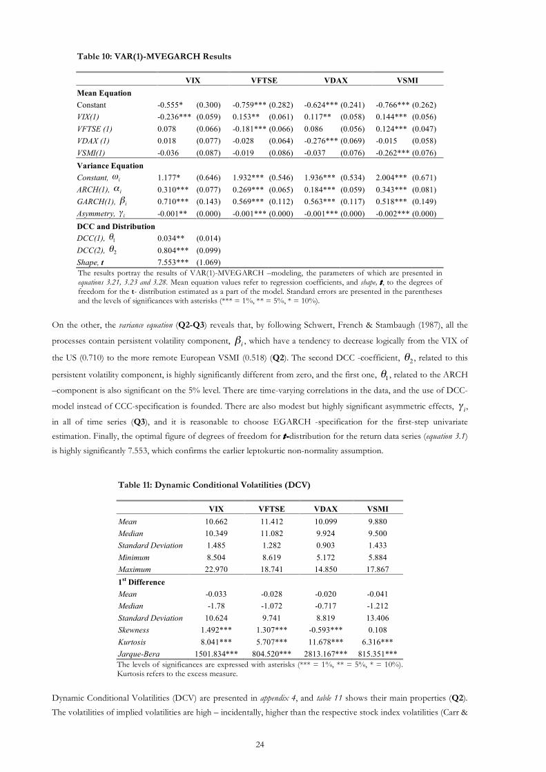
24
Table 10: VAR(1)-MVEGARCH Results
VIX VFTSE VDAX VSMI Mean Equation Constant -0.555* (0.300) -0.759*** (0.282) -0.624*** (0.241) -0.766*** (0.262) VIX(1) -0.236*** (0.059) 0.153** (0.061) 0.117** (0.058) 0.144*** (0.056) VFTSE (1) 0.078 (0.066) -0.181*** (0.066) 0.086 (0.056) 0.124*** (0.047) VDAX (1) 0.018 (0.077) -0.028 (0.064) -0.276*** (0.069) -0.015 (0.058) VSMI(1) -0.036 (0.087) -0.019 (0.086) -0.037 (0.076) -0.262*** (0.076) Variance Equation Constant,
!
"i 1.177* (0.646) 1.932*** (0.546) 1.936*** (0.534) 2.004*** (0.671)
ARCH(1),
!
"i 0.310*** (0.077) 0.269*** (0.065) 0.184*** (0.059) 0.343*** (0.081)
GARCH(1),
!
"i 0.710*** (0.143) 0.569*** (0.112) 0.563*** (0.117) 0.518*** (0.149)
Asymmetry,
!
"i -0.001** (0.000) -0.001*** (0.000) -0.001*** (0.000) -0.002*** (0.000)
DCC and Distribution DCC(1),
!
"1 0.034** (0.014)
DCC(2),
!
"2 0.804*** (0.099)
Shape, t 7.553*** (1.069) The results portray the results of VAR(1)-MVEGARCH –modeling, the parameters of which are presented in equations 3.21, 3.23 and 3.28. Mean equation values refer to regression coefficients, and shape, t , to the degrees of freedom for the t- distribution estimated as a part of the model. Standard errors are presented in the parentheses and the levels of significances with asterisks (*** = 1%, ** = 5%, * = 10%).
On the other, the variance equation (Q2-Q3) reveals that, by following Schwert, French & Stambaugh (1987), all the
processes contain persistent volatility component,
!
"i, which have a tendency to decrease logically from the VIX of
the US (0.710) to the more remote European VSMI (0.518) (Q2). The second DCC -coefficient,
!
"2, related to this
persistent volatility component, is highly significantly different from zero, and the first one,
!
"1, related to the ARCH
–component is also significant on the 5% level. There are time-varying correlations in the data, and the use of DCC-
model instead of CCC-specification is founded. There are also modest but highly significant asymmetric effects,
!
"i,
in all of time series (Q3), and it is reasonable to choose EGARCH -specification for the first-step univariate
estimation. Finally, the optimal figure of degrees of freedom for t -distribution for the return data series (equation 3.1)
is highly significantly 7.553, which confirms the earlier leptokurtic non-normality assumption.
Table 11: Dynamic Conditional Volatilities (DCV)
VIX VFTSE VDAX VSMIMean 10.662 11.412 10.099 9.880Median 10.349 11.082 9.924 9.500Standard Deviation 1.485 1.282 0.903 1.433Minimum 8.504 8.619 5.172 5.884Maximum 22.970 18.741 14.850 17.8671st Difference
Mean -0.033 -0.028 -0.020 -0.041Median -1.78 -1.072 -0.717 -1.212Standard Deviation 10.624 9.741 8.819 13.406Skewness 1.492*** 1.307*** -0.593*** 0.108Kurtosis 8.041*** 5.707*** 11.678*** 6.316***Jarque-Bera 1501.834*** 804.520*** 2813.167*** 815.351***The levels of significances are expressed with asterisks (*** = 1%, ** = 5%, * = 10%). Kurtosis refers to the excess measure.
Dynamic Conditional Volatilities (DCV) are presented in appendix 4, and table 11 shows their main properties (Q2).
The volatilities of implied volatilities are high – incidentally, higher than the respective stock index volatilities (Carr &

25
Wu 2006, 19-20; Moran & Dash 2007, 97; Szado 2009, 10) – the means and standard deviations are decreasing all the
way from the USA to the more remote European markets, and the largest peaks are consistently upwards. These
deviations from the mean are abrupt and extreme, but of short term – even during the subprime crisis only the VIX
has a longer term elevated DCV levels. This means that the markets are fast and efficient in adjusting to new
information. Because of the mean reversion of the time series, the first differences (table 11) are also of interest. All
the distributions are leptokurtic, non-normal. Excluding the VSMI and the negatively skewed VDAX, the rest are
positively skewed, which means the positive changes are larger in general than the negative ones. Then, the negative
means and medians differ quite a bit, and the standard deviations are extensive.
Dynamic Conditional Correlations (DCC) of appendix 5 are high and extremely stable (Q2), as also presented in table
12. The means and medians coincide, and the standard deviations of are small. 1st differences confirm non-normal,
leptokurtic behavior for all time series. All statistically significant measures of skew are negative. The changes of the
mean in the correlations are time wise longer than those of DCVs, and the ends of those peaks revert back to their
means smoothly. New information arriving in a market leads to an abrupt change in the DCC, as it takes some time
for the information to spill over. The spillover then gradually mitigates the change in DCC between the markets.
These changes in the correlations in the face of the crises are still surprisingly small, although the correlations seem
to have a tendency to change in the context of extensive shocks. Also, most correlations have a tendency to fall more
than to grow, in the face of subprime crises, excluding the VFTSE-VDAX, which is exceptional by many ways. The
Dynamic Conditional Correlations 2 –table of appendix 5 show that regional and local European overall correlations
are higher than the global ones with VIX.
Table 12: Dynamic Conditional Correlations (DCC)
CORRELATIONS VIX-VFTSE VIX-VDAX VIX-VSMI VFTSE-VDAX VFTSE-VSMI VDAX-VSMIMean 0.734 0.767 0.698 0.866 0.821 0.853Median 0.735 0.767 0.696 0.866 0.820 0.853Standard Deviation 0.031 0.025 0.034 0.0173 0.0260 0.020Minimum 0.573 0.682 0.534 0.813 0.647 0.740Maximum 0.839 0.868 0.818 0.924 0.888 0.9091st Difference
Mean -0.005 -0.002 0.000 0.000 -0.000 0.000Median -0.091 -0120 -0.086 -0.005 -0.026 -0.001Standard Deviation 2.334 1.909 2.669 1.064 1.739 1.212Skewness -0.499*** 0.029 -0.536*** -0.057 -4.877*** -0.927***Kurtosis 16.369*** 10.042*** 14.399*** 7.070*** 72.417*** 12.414***Jarque-Bera 5491.053*** 2059.021*** 4256.6240*** 1020.748*** 109012.585*** 3216.328***The levels of significances are expressed with asterisks (*** = 1%, ** = 5%, * = 10%). Kurtosis refers to the excess measure.
Residuals diagnostics. It is essential to study the properties of the MGARCH –residuals, as they convey information
about the fit and robustness of the model. They affect the choice of the final model, as the chase after the most
robust, efficient and parsimonious model is cyclical and repetitive by nature. Still, residual testing is not completely
reliable as is, because many of the asymptotic properties of the DCC-model used are unknown, and formal critical
values may not be available for the test statistics (Bauwens et al. 2006, 102). Thus, the final decisions about the most
appropriate model are made based on all information available. The results (table 13) show that all the time series are
still positively skewed, leptokurtic, and the Jarque-Bera Null-hypotheses of normality can be rejected, as was
predicted by theory (ibid., 96). Autocorrelations and heteroscedasticities, measured by Ljung-Box Portmanteau tests,
and different ARCH-effects are non-existent but may suffer from asymptotical impreciseness.

26
Table 13: Residuals Diagnostics I
VIX VFTSE VDAX VSMIObservations 491 491 491 491Minimum -2.998 -3.046 -3.597 -3.166Maximum 5.470 4.520 4.828 4.207Mean 0.071 0.072 0.067 0.080Standard Deviation 1.012 1.030 1.039 1.036Skewness 0.740*** 0.661*** 0.734*** 0.447***Kurtosis 1.955*** 1.501*** 2.265*** 1.095***Jarque-Bera 123.041*** 81.926*** 149.040*** 40.862***LB(4) 4.333 4.543 3.994 3.863LB(8) 12.579 10.487 6.882 10.430LB(12) 16.473 12.120 13.566 12.639LB2(4) 0.628 0.804 3.539 1.079LB2(8) 4.396 7.374 5.083 4.266LB2(12) 6.255 9.440 5.558 6.878ARCH(4) 0.160 0.194 0.866 0.271ARCH(8) 0.507 0.831 0.617 0.545ARCH(12) 0.484 0.680 0.432 0.572ARCH2(4) 0.026 0.160 0.100 0.134ARCH2(8) 0.042 0.131 0.087 0.133ARCH2(12) 0.047 0.139 0.108 0.153
The levels of significances are presented with asterisks (*** = 1%, ** = 5%, * = 10%). Kurtosis is calculated as a standard excess measure. Ljung-Box (LB) and the test of ARCH -effects results are expressed as joint tests for different lags, and also for squared values (LB2 & ARCH2).
The residuals of one-mean-equation-lag model (suggested by BIC) are more robust compared to those of three-lag
model (suggested by AIC and HQ). The Ljung-Box and ARCH-effect results are slightly different but not generally
better for either of the models. As an outcome, the one-lag model is chosen that also leads to more meaningful
modeling results presented in table 10. Finally, there is no asymmetry left in the residuals tested (table 14), measured
by Engle–Ng –test.
Table 14: Residuals Diagnostics II
Variable VIX VFTSE VDAX VSMIConstant 1.152***(0.205) 1.056***(0.192) 1.193***(0.209) 1.222***(0.183)
!
St"1
" -0.250 (0.300) 0.251 (0.292) 0.112 (0.317) -0.134 (0.274)
!
St"1
"ut"1
2 -0.008 (0.258) 0.407 (0.247) 0.401 (0.265) 0.208 (0.221)
!
St"1
+ut"1
2 -0.003 (0.176) 0.067 (0.166) -0.059 (0.179) -0.006 (0.161)
Joint-
!
" 2 1.655 3.149 2.767 3.484Standard errors are presented in the parentheses and the levels of significances with asterisks (*** = 1%, ** = 5%, * = 10%). The coefficients coincide with those in equation (3.9), while constant does not have economic meaning. The joint test statistics follow Chi2 -distribution.

27
6. DISCUSSION
The results speak for wider international systemic behavior of the underlying Western stock markets. This
increasingly complex phenomenon is often reported as a consequence of increased financial globalization. The
results reveal only unidirectional volatility spillovers (Q1 ) between the VIs, while the American VIX seems to be the
central source of the volatility spillovers, while the VFTSE behaves as a local source with respect to the VSMI. These
findings, combined with the fact that the VDAX does not have spillover with the VFTSE and VSMI, describe the
nature of the spillovers very well. While geographical (proximity), cultural and shared real economy factors seem to
contribute higher correlation and shared market behavior, the financial relationships seem to contribute spillovers.
By interpreting VIs as indicators of the markets, the UK and Germany have important trade relationships with the
USA and it is natural that spillovers exist between these markets. The size and global importance might explain why
the spillovers are solely outwards from the US, as also found by Theodossiou & Lee (1993). The lack of spillovers
between the highly correlated main European markets can be explained as a sign of the unified nature of regional
markets. The markets evolve so closely with each other that there are no follow-ups at the moment t-1. The daily
data would be likely to reveal spillovers, but as stated could suffer from the effects of non-synchronous trading. The
high correlation between the indices rules out the possibility that the markets were not related at all. The
unidirectional spillovers from the VIX confirm the central position of the US market as a source of the new market
information globally. In this framework, the Swiss market seems to be a local player closely integrated (correlation)
with the German market, but in the UK’s tow (spillovers). As a summary, the results show that volatility spillovers
do exist.
The VAR-MVEGARCH -specification reveals that the volatilities and correlations include dynamic conditional
effects (Q2 ). The behaviors of the DCV levels are not surprising per se, as the volatilities of VIs, i.e. volatilities of
volatilities, have traditionally been high compared to the volatilities of their respective stock indices (Moran & Dash
2007, 97). Still, VIs essentially serve as a fear gauge of the market, not only indicating the stock market plummets,
but also indicating the overall confidence of the market (Moran & Dash 2007, 97; Whaley 2000). As a consequence,
the changes are short term and abrupt, portraying sentiments of emerging new information related to the underlying
index. In terms of hedging, the deviations from the mean reversions target are short-term on the 1st difference return
level, and thus appropriate for catastrophe hedging, where large and sudden changes take place on the market. Still, it
must be remembered that the indices also portray longer term implied volatility levels, as can be seen by studying the
appendix 2. Further, the markets in question are highly correlated. Short-term fluctuations still exist, as the spillovers
do not correct the volatility changes immediately, but smoothly over time. Together with earlier spillover findings,
this confirms that volatility spillovers are essentially information transmission (Stoll & Whaley 1990; Chan, Chan &
Karolyi 1991; French & Roll 1986).
In terms of diversifying the volatility investment, investing even in one single VI may work, as high correlations limit
the benefits of diversification – especially if perfect short-term hedging is not important. The problem is that
although VIs offer good catastrophe hedging i.e. to compensate for large negative shocks of the underlying stock
index (Moran & Dash 2007, 104), even small drops in the correlations in the face of the crisis may become crucial,
when the original shock is extensive. Thus, if the local VI truly represents the risk level, it is likely to offer better
protection for short-term fluctuations than the foreign VIs. There are exceptions to the rule such as between the
VFTSE-VDAX and the VDAX-VSMI. These VIs are part of the same regional market area, highly correlated, and
the problem causing spillovers are few. All in all, this might explain why the highest overall correlations are found in
the highly integrated European market area, while the formal EU itself is not the essential factor.

28
There are small but statistically significant volatility asymmetries captured by the model used (Q3 ) in every single
index. This means that the nature of past news is of importance. The preliminary finding for the VIX by Carr & Wu
(2006, 18-19) is confirmed and extended. This finding is important in the economic sense as it shows that this
asymmetry seems to be a common property of VIs, although explaining this property further lies beyond this study.
The asymmetries in the volatilities of implied volatilities could be caused by the leverage effects of the underlying
stock indices (Black 1976), or by some other reasons (Bekaert & Wu 2000; Black 1976; Campbell & Hentschel 1992;
Campbell & Kyle 1993; Haugen et al. 1991).
Other findings. In the long term, the stability of volatility (and correlations) as a measure is confirmed. In any case, VIs
are not free from biases either, and might explain at least some of the bias Jiang & Tian (2007) have found. In the
shorter term, the self-effects of the VIs, represented by the 1st lags in the mean equation, are highly significantly
negative and relatively large. In other words, the historic values have a geometrically decreasing negative
autocorrelation relationship with the new events that is a natural finding. The distributions of the 1st difference
returns are leptokurtic with thick tails and are thus non-normal. Finally, the VIs contain day effects, although not
traded as is. Besides trading (Carr & Wu 2006), the day effects can most likely be traced back to the underlying stock
indices.
6.1. Robustness of the results
There are two issues, related to the robustness of the results, repeatedly raised in the literature, a) the misspecified model
(Hoover & Siegler 2008a), and b) the difficulty of strict division between statistical and economic interpretation of the data
(Hoover & Siegler 2008b). The latter states that statistical hypotheses are not always either true or false (Leamer
2004) leading to reliability problems.
A misspecified model could lead to completely biased test statistics, which in turn would confirm nonsense results.
Feinstein & Thomas (2002) speak about this aspect more closely. They remind us that if there is no symmetry of
errors (or the study is based on a biased model without asymptotic properties), the results can be seriously biased
without the researcher noticing it. This leads us to the capabilities of the researcher, as the only way around the
problem, is the researchers ability to evaluate the appropriateness of the models used (also Horowitz 2004). Hence,
the economic reasoning of the data must be observed more widely, and it must depend on the situation. The original
figures are made available, so that the reader can make his or her own conclusions. In the context of the model,
Engle’s (2002) DCC-model allows only real number specifications for the dynamics of the correlations. It is possible
that the model does not reveal, misleadingly specifies, the dynamics of correlations (Bauwens et al. 2006). The results
also show a small but statistically significant asymmetry for all the time series, not found in the descriptive statistics
(table 7). This finding may reflect the fact that the model does not fit the data perfectly. VARMA-GARCH does
converge, so it cannot be used as an alternative. In practice, the most important decision is related to the choice of
lags for the mean equation of the MVEGARCH -model.
Difference between statistical and economic interpretation. Errors are indispensable in economic research, while Kirzner (1999,
125-131) pays attention to “correctly calculated imperfection”, which means reaching appropriate results with respect to
the relevant search costs. Better results would increase error. Ethridge (2004, 47-49) explains that the error is
unavoidable, but non-harmful if its nature and role in the study is correctly understood and tested. Hoover and
Siegler (2008a) notice that economic interpretation is subjective by nature to some extent. Berg (2004) offers as a
solution, that Null- and Alternative hypotheses, would be augmented with No-decision hypothesis, which would
help in those tricky cases, when conclusions can not be drawn (e.g. if economic and statistical statistics do not speak

29
the same language.) Horowitz (2004) highlights the importance of what “constitutes good practice in handling
random sampling errors” and concludes that testing is not always reliable anyway, and that sometimes only the
existence of a phenomenon is enough for conclusions, while significance on certain specified level is not an essential
property. As long as the problem is poorly specified, the discussion does not lead further. Hence, lots of attention is
paid to the problem setting and interpretation of the results, and the ethics behind the interpretation (Wooldridge
2004). The economic and statistical results of the study are largely alignedx, but the statistical results presented in the
tables and figures are kept separate from the economic reasoning. Hence, the reader can draw his or her own
conclusions from the results.
Volatility as a theoretical asset. All conclusions about true volatilities between the markets must be drawn remembering
the fact that the VIs are treated here as assets. It is also reasonable to ask, to what degree the results can be applied
to practical management of volatility assets? Investing in VIs takes place through derivatives, the time series of which
may behave differently from but are related to those of underlying VIs (Nossman & Wilhelmsson 2008), or they are
not possible at all. This causes evident problems, not easily answered, highlighting the importance of treating VIs as
individual assets. Because of varying properties and poor availability of the data accessible for multivariate studies, it
is most reasonable to use VIs themselves, not the derivatives, as data. This approach has been used in the context of
VI –research also earlier – most notably by Black (2006). It is still of most importance that the limitations of such
results are remembered.
Other issues. The modeling took place by using first difference returns and weekly values. Use of the returns lead
inevitably to loss of information in the results. Still, the models do not converge when log-level values are used, and
as volatility is treated as an asset, it is reasonable to study returns of the asset instead of VI levels as is. The use of
weekly values is founded, in order to avoid the effects of non-synchronous trading, although it may hide some of the
short-term spillovers. The sample size is large enough for reliable GARCH estimation, even using weekly values
through the time window. Another topical data-related question relates to the questionable mean reversion of the
data series, revealed by the preliminary research. It is theoretically unfounded to assume a volatility series containing
unit roots – the view supported by the most sophisticated unit root test. On the 1st difference returns level, the
hypotheses of unit roots are rejected by all tests used. As the time series are not cointegrated, the VECM-parameters
are unnecessary.
6.2. Further Research
The field studied here is developing rapidly, and new assumptions and approaches for modeling are established
constantly. These include modeling options on the VIs by using jump-diffusion models (Sepp 2008; Carr & Wu
2006, 18) and introducing a whole new class of information derivatives (Soklakov 2008). Therefore new approaches
will be needed in establishing sound research settings. In the context of this study, the same methodology could be
applied to study VIs in one specific area, such as the Euro currency area, in order to compare the results with respect
to this one. In the future when time series allow, the same methodology could be used to study developing and Asian
markets, many of which have recently introduced their own VIs, and which (more often than not) are specified
similar to that of the VIX. It would be also interesting to conduct similar studies on derivatives written on different
VIs, as soon as data become available. Such studies would shed light on how investing in and trading of implied
volatilities through derivatives (e.g. Black 2006; Sepp 2008), is connected between different markets in practice, and
also reveal differences between the markets of VIs and their respective derivatives. Finally, the reasons for the day
effects could be studied: a) the impact of trading is theoretically interesting, as the derivatives based volatilities are
generally considered a relatively stable and reliable measure of risk (e.g. Hull 2009), and b) the impact of underlying
stock indices and their relationships to the leverage effects would be worth studying.

30
6.3. Conclusions
All in all, the volatility indices of Western developed markets, are highly correlated, and carry the unified message of
uncertainty in the respective markets in the long run. Even more so on the regional and local level. Theoretical
investments in the several volatility indices would yield only limited diversification benefits in the Western world.
Depending on the case, it may then be possible to use only one or a few VIs as a hedging tool for an international
developed market portfolio, on the condition that the spillover relationships – affected by the financial market
relations – between the markets in question are known. In the light of the findings of this study, it is not surprising
that the VIX is currently the most popular volatility index among investors. From the variance-covariance (or
correlation) matrix standpoint, there are relatively small, but significant dynamic effects over time. In the short run,
the dynamic relationships cause temporary differences, and as VI –based hedging strives especially for crash
protection, hedging using the local market index would bring the greatest efficiency. Otherwise, the changing (most
often decreasing) correlations in the face of crisis (as during the subprime crisis) may jeopardize some of the hedge.
Because of the fast changes in the VIs volatility, it is not necessarily so that short delay in liquidizing would fix the
problem. This very fact applies also to the use of VIs as the market indicator. Hence, it is crucial to use the local VI
signaling the short-term uncertainty of the market, and variance swap levels. Naturally, this is of utmost importance,
if VIs are used as market timing tools. Finally, there are information transmissions between the markets – spillovers
running unidirectionally from the US VIX to the other VIs.

31
REFERENCES
Primary and secondary sources are not separated in the list.
Aboura, S. (2003). International Transmission of Volatility: A study on the volatility indexes VX1, VDAX and VIX.
Working paper: ESSEC Business School.
Ahoniemi, K. (2008). Modeling and Forecasting the VIX index. Working paper: Helsinki School of Economics and
HECER.
Altman, M. (2004). Statistical significance, path dependency, and the culture of journal publication. Journal of Socio-
Economics, 33, pp. 651-663.
Andersen, T. & Bollerslev T. (1997). Heterogeneous information arrivals and return volatility dynamics: Uncovering
the long run in high frequency returns. Journal of Finance, 52, pp. 975-1006.
Andrews, D.W.K. (1991). Heteroskedasticity and Autocorrelation Consistent Covariance Matrix Estimation.
Econometrica, 59, pp. 817-858.
Apolinario, R. M. C. & Caro, A. R. (2006). Day of the Week Effect on European Stock Markets. International
Research Journal of Finance and Economics, 2, pp. 53-70.
Arak, M. (2006). The VIX and VXN volatility measures: Fear gauges or forecasts? Derivatives Use, Trading &
Regulation, 12, pp. 14-27.
Backhouse, R. E. (1998). Explorations in Economic Methodology: From Lakatos to empirical philosophy of science.
Routledge: London.
Banerjee, P.S., Doran, J.S. & Peterson, D.R. (2006). Implied Volatility and Future Portfolio Returns. Journal of Banking
& Finance, 31, pp. 3183-3199.
Bauwens, L., Laurent, S. & Rombouts, J. V. K. (2006). Multivariate GARCH models: A survey. Journal of Applied
Econometrics, 21, pp. 79-109.
Becker, R., Clements, A.E. & McClelland, A. (2009). The jump component of S&P 500 volatility and the VIX index.
Journal of Banking & Finance, 33, pp. 1033-1038.
Becker, R., Clements, A.E. & White, S.I. (2007). Does implied volatility provide any information beyond that
captured in model-based volatility forecasts? Journal of Banking & Finance, 31, pp. 2535-2549.
Bekaert, G. & Wu, G. (2000). Asymmetric Volatilities and Risk in Equity Markets. Review of Financial Studies, 13, pp. 1-
42.
Berg, N. (2004). No-decision classification: an alternative to testing for statistical significance. Journal of Socio-
Economics, 33, pp. 631-650.
Billio, M., Caporin, M., & Gobbo, M. (2003). Block Dynamic Conditional Correlation Multivariate GARCH Models.
Greta Working Paper. 03.03.
Black, F. (1976). Studies of Stock Price Volatility Changes. In Proceedings of the 1976 American Statistical Association,
business and Economical Statistics Section., pp. 177-181. American Statistical Association: Alexandria, VA.
Black, F. (1989). How We Came Up With the Option Pricing Formula. Journal of Portfolio Management, 15, pp. 4-8.
Black, F. & Scholes, M. (1973). The Pricing of Options and Corporate Liabilities. Journal of Political Economy, 81, pp.
637-659.
Black, K. H. (2006). Improving Hedge Fund Risk Exposures by Hedging Equity Market Volatility, or How the VIX
Ate My Kurtosis. The Journal of Trading, 1, pp. 6-15.
Bollerslev, T. (1990). Modelling the Coherence in Short-Run Nominal Exchange Rates: A Multivariate Generalized
ARCH Approach. Review of Economics and Statistics, 72, pp. 498-505.

32
Bollerslev, T., Engle, R.F., & Wooldridge, J.M. (1988). A Capital-Asset Pricing Model with Time-Varying
Covariances. Journal of Political Economy, 96, pp. 116-131.
Booth, G., Martikainen, T. & Tse, Y. (1997). Price and Volatility Spillover in Scandinavian Stock Markets. Journal of
Banking and Finance, 21, pp. 811-823.
Brooks, C. (2008). Introductory Econometrics for Finance. 2nd Ed. Cambridge University Press,
Campbell, J.Y. & Hentschel. L. (1992). No News Is Good News: An Asymmetric Model of Changing Volatility in
Stock Returns. Review of Economic Studies, 31, pp. 281-318.
Campbell, J.Y. & Kyle, A.S. (1993). Smart Money, Noise Trading and Stock Price Behavior. Review of Economic Studies,
60, pp. 1-34.
Canina, L. & Figlewski, S. (1993). The Information Content of Implied Volatility. Review of Financial Studies, 6, pp.
659-681.
Carr, P. & Wu, L. (2006). A Tale of Two Indices. The Journal of Derivatives, 13, pp. 13-29.
CBOE. (2009). VIX White Paper. <URL: http://www.cboe.com/micro/vix/vixwhite.pdf >. May 5th, 2010.
Chan, K., Chan, K.C. & Karolyi, G.A. (1991). Intraday volatility in the stock index and stock index futures markets.
Review of Financial Studies, 4, pp. 657-684.
Chang, E., Pinegar, M. & Ravichandran, R. (1993). International Evidence on the Robustness of the Day-of-the-
Week Effect. Journal of Financial and Quantitative Analysis, 28, pp. 497-513.
Christensen, B.J. & Prabhala, N.R. (1998). The Relation between Implied and Realized Volatility. Journal of Financial
Economics, 50, pp. 125-150.
Cipollini, A. & Manzini, A. (2007). Can The Vix Signal Market Direction?: An Asymmetric Dynamic Strategy.
Working Paper: University of Milan-Bicocca.
Cochrane, J. H. (2005). Writing Tips for Ph.D. Students. Graduate Business School of Business, University of
Chicago.
Copeland, M. & Copeland T. (1998). Leads, lags and trading in global markets. Financial Analyst Journal, 54, pp. 70-80.
Cross, F. (1973). The Behavior of Stock Prices on Fridays and Mondays. Financial Analyst Journal. (Nov.-Dec.), pp.
67-69.
Day, T.E. & Lewis, C.M. (1988). The Behavior of the Volatility Implicit in Option Prices. Journal of Financial
Economics, 22, pp. 103-122.
Ederington, L.H. & Guan, W. (2002). Why Are Those Options Smiling? Journal of Derivatives, 10, pp. 9-34.
Eicker, F. (1967). Limit Theorems for Regressions with Unequal and Dependent Errors. In Proceedings of the Fifth
Berkeley Symposium on Mathematical Statistics and Probability. pp. 59-82. Eds. L.LeCam & J. Neyman. University
of California Press.
Elliot, G. & Granger, C. W. J. (2004). Evaluating significance: comments on “size matters”. Journal of Socio-Economics,
33, pp. 547-550.
Engle, R. F. (1982). Autoregressive Conditional Heteroskedasticity with Estimates of Variance of United Kingdom
Inflation. Econometrica, 50, pp. 987-1007.
Engle, R. F. (2001). GARCH 101: The Use of ARCH/GARCH Models in Applied Econometrics. Journal of Economic
Perspectives, 15, pp. 157-168.
Engle, R. F. (2002). Dynamic Conditional Correlation: A Simple Class of Multivariate Generalized Autoregressive
Conditional Heteroskedasticity Models. Journal of Business & Economic Statistics, 20, pp. 339-350.
Engle, R.F. & Bollerslev, T. (1986). Modeling the Persistence of Conditional Variances. Econometric Reviews, 5, pp. 1-
50.
Engle, R. F. & Kroner, F. K. (1995). Multivariate Simultaneous Generalized ARCH. Economic Theory, 11, pp. 122-150.
Engle, R. F. & Ng, V. K. (1993) Measuring and Testing the Impact of News on Volatility. Journal of Finance, 48, pp.
1749-1778.

33
Eraker, B., Johannes, M. S., & Polson, N.G. (2003) The Impact of Jumps in Equity Index Volatility and Returns.
Journal of Finance, 58, pp. 1269-1300.
Erb, C. B., Harvey, C. R. & Viskanta, T. E. (1994). Forecasting International Equity Correlations. Financial Analyst
Journal, pp. 32-45.
Ethridge, D. (2004). Research Methodology in Applied Economics. 2nd Ed. Blackwell: Oxford.
Fama, E. F. (1965). The Behavior of Stock Market Prices. Journal of Business, 38, pp. 34-105.
Federal Reserve System. FRB: Statistics and Historical Data. <URL: http://www.federalreserve.gov/econresdata
/releases/statisticsdata.htm>. April 22th, 2010.
Feinstein, C. H. & Thomas, M. (2002). A Plea for Errors. Historical Methods, 35, pp. 155-165.
Foster, F. D. & Viswanathan, S. (1990). A Theory of the interday variations in Volume, Variances, and Trading Cost
in Securities Market. Review of Financial Studies, 3, pp. 539-624.
Foster, F. D. & Viswanathan, S. (1993). Variations in Trading Volume, Return Volatility, and Trading Cost: Evidence
From Recent Price Formation Models. Journal of Finance, 48, pp. 187-211.
French, K. (1980). Stock Returns and the Weekend Effect. Journal of Financial Economics, 8, pp. 55-69.
French, K. R. & Roll, R. (1986). Stock Return Variances: The Arrival of Information and the Reaction of Traders.
Journal of Financial Economics, 17, pp. 5-26.
Haugen, R.A., Talmor, E. & Torous, W.N. (1991). The Effect of Volatility Changes on the Level of Stock Prices and
Subsequent Expected Returns. Journal of Finance, 46, pp. 985-1007.
Hull, J.C. (2007). Options, futures, and other derivatives. 7th ed. Prentice Hall: London.
Gaines, K. (2002). Writing a Master’s Thesis or dissertation Proposal. Graduate Writing Resource, University of
Arizona. http://www.gwr.arizona.edu/
Gatheral, J. (2006). The Volatility Surface; A Practitioner’s Guide. Wiley: Hoboken, NJ.
Gay, G. & Kim, T. (1987). An Investigation into Seasonality in the Futures Market. Journal of Futures Markets, 7, pp.
169-181
Gonzalez-Perez, M. T. & Guerrero, D. E. (2009). The Daily Closing VIX Data for 2008 Reveal Unrecognized
Properties. SSRN / Northwestern University: Working Paper.
Gourieroux, C. & Jasiak, J. (2001). Financial Econometrics: Problems, Models, and Methods. Princeton University
Press.
Graham, J. R. & Harvey, C. R. (2009). The Equity Risk Premium amid a Global Financial Crisis. Duke University:
Working Paper.
Grant, M., Gregory, K. & Lui, J. (2007). Volatility as an Asset. Goldman Sachs Global Investment Research. (Nov.
15th).
Hirsjärvi, S., Remes P. & Sajavaara P. (1997). Tutki ja kirjoita. (A Manual for Academic Research and Writing). 6.-8.
Ed. Helsinki: Tammi.
Hoover, K. D. & Siegler, M. V. (2008a). Sound and fury: McCloskey and significance testing in economics. Journal of
Economic Methodology, 15, pp. 1-37.
Hoover, K. D. & Siegler, M. V. (2008b). The Rhetoric of ’Signifying nothing’: a rejoinder of Ziliak and McCloskey.
Journal of Economic Methodology, 15, pp. 57-68.
Horowitz, J. L. (2004). Comments on “Size Matters”. Journal of Socio-Economics, 33, pp. 551-554.
Hsu, S.D.H. & Murray, B.M. (2007). On the volatility of volatility. Physica A: Statistical Mechanics and its Applications,
380, pp. 366-376.
Hull, J. C. (2009). Options, Futures, and Other Derivatives. 7th Ed. Pearson-Prentice Hall: New Jersey.
Hull, J. C. & White, A. (1987). The Pricing of Options on Assets with Stochastic Volatilities. Journal of Finance, 42, pp.
281-300.
Hull, J. C. & White, A. (1988). An Analysis of the Bias in Option Pricing Caused by a Stochastic Volatility. Advances
in Futures and options Research, 3, pp. 27-61.

34
Jiang, G.J. & Tian Y.S. (2007). Extracting Model-Free Volatility from Option Prices: An Examination of VIX index.
Journal of Derivatives, 14, pp. 35-60.
Johansson, A. C. & Ljungwall, C. (2009). Spillover Effects Among the Greater China Stock Markets. World
Development, 37, pp. 839-851.
Johnson, G. L. (1986). Research Methodology for Economists: Philosophy and Practice. Macmillan: New York.
Johnston, J. & DiNardo, J. (1997). Econometric Methods. 4th Ed. MacGraw-Hill: Singapore.
Kirzner, I. M. (1999). Economists and the Correction of Error. What Do Economists Contribute? Ed. Klein & Palgrave.
CATO Institute: London.
Kiymaz, H. & Berument, H. (2003). The Day of the Week Effect on Stock Market Volatility and Volume:
International Evidence. Review of Financial Economies, 12, pp. 363-380.
Koutmos, G. & Booth, G. (1995). Asymmetric Volatility Transmission in International Stock Markets. Journal of
International Money and Finance, 14, pp. 747-762.
Keim, D. B. & Stambaugh, F. (1984). A Further Investigation of Weekend Effects in Stock Returns. Journal of
Finance, 39, pp. 819-840.
Kremer, M. (200?). Writing Papers: A Checklist. http://www.economics.harvard.edu/faculty/kremer/files
/checklist.pdf
Lakonishok, J. & Levi, M. (1982). Weekend Effect in Stock Return: A Note. Journal of Finance, 37, pp. 883-889).
Leamer, E. E. (2004). Are the roads red? Comments on “Size Matters”. Journal of Socio-Economics, 33, pp. 555-
557.
Lee, J. & Strazicich, M. (2003). Minimum LM Unit Root Test with Two Structural Breaks. Review of Economics and
Statistics, 85, pp. 1082–1089.
Lee, J. & Strazicich, M. (2004). Minimum LM Unit Root Test with One Structural Break. Appalachian State
University. Working Paper.
Lin, W., Engle, R. & Ito, T. (1994). Do Bulls and Bears Move Across Borders? – International Transmission of
Stock Volatility. Review of Financial Studies, 7, pp. 507-538.
Ling, S. & McAleer, M. (2003). Asymptotic Theory For a Vector ARMA-GARCH Model. Econometric Theory, 19, pp.
280-310.
Ljung, G. M. & Box, G. E. P. (1978). On a Measure of Lack of Fit in Time Series Models. Biometrika, 65, pp.297-303.
Longin, F. & Solnik, B. (1995). Is the Correlation in International Equity Returns Constant: 1960-1990. Journal of
International Money and Finance, 14, pp. 3-26.
Majmudar, U. & Banerjee, A. (2004). VIX Forecasting. Working Paper.
Manera, M., McAleer, M. & Grasso, M. (2006). Modelling time-varying conditional correlations in the volatility of
Tapis oil spot and forward returns. Applied Financial Economics, 16, pp. 525-533.
McCloskey, D. N. (1998). The Rhetoric of Economics. 2nd Ed. The University of Wisconsin Press.
McCloskey, D. N. (2002). The Secret Sins of Economics. Prickly Paradigm: Chicago.
McCloskey, D. N. & Ziliak, S. T. (1996). The Standard Error of Regressions. Journal of Economic Literature, 34, pp. 97-
114.
McCloskey, D. N. & Ziliak, S. T. (2004). Size Matters: The Standard Error of Regressions in the American
Economic Review. Journal of Socio-Economics, 33, pp. 527-546.
McCloskey, D. N. & Ziliak, S. T. (2008). Signifying Nothing: Reply to Hoover and Siegler. Journal of Economic
Methodology, 34, pp. 39-55.
Merton, R. C. (1973). Theory of Rational Option Pricing. Bell Journal of Economics and Management Science, 4, pp. 141-
183.
Merton, R. C. (1976). Option Pricing When Underlying Stock Returns Are Discontinuous. Journal of Financial
Economics, 3, pp. 125-144.

35
Moran, M.T. & Dash, S. (2007.) VIX Futures and Options: Pricing and Using Volatility Products to Manage
Downside Risk and Improve Efficiency in Equity Portfolios. The Journal of Trading, 2, pp. 96-105.
Mäki, U., Gustafsson, B. & Knudsen, C. (1993). Rationality, Institutions, and Economic Methodology. Routledge:
London.
Nelson, D.B. (1991). Conditional Heteroskedasticity in Asset Returns: A New Approach. Econometrica, 59, pp. 347-
370.
Newey, W. K. & West, K. (1987). A Simple Positive Semi-Definite, Heteroskedasticity and Autocorrelation
Consistent Covariance Matrix. Econometrica, 55, pp. 703-708.
Nossman, M. & Wilhelmsson, A. (2008). Is the VIX Futures Market Able to Predict the VIX Index?: A Test of the
Expectation Hypothesis. Lund University: Working Paper.
Osborne, M. (1962). Periodic Structure in the Brownian Motion of Stock Prices. Operations Research, 10, pp. 267-290.
Press, W.H., Flannery, B.P., Teukolsky, S.A. & Vettering, W.T. (1988). Numerical Recipes in C. Cambridge
University Press: New York.
Rogalski, R. J. (1984). New Findings Regarding Day-of-the-Week Returns over Trading and Nontrading Periods: A
Note. Journal of Finance, 35, pp. 461-468.
Ross, S.A. (1989). Information and volatility: The no-arbitrage martingale approach to timing and resolution
irrelevancy. Journal of Finance, 44, pp. 1-17.
Ryan, B., Scapens, R.W. & Theobald, M. (2002). Research Method & Methodology in Finance and Accounting. 2nd
Edition. Thomson: London.
Satchell, S. & Knight, J. L. (Eds). (2002). Forecasting Volatility in Financial Markets. 2nd Ed. Butterworth-
Heinemann: Oxford.
Schmidt, P. & Phillips, P.C.B. (1992). LM Tests for a Unit Root in the Presence of Deterministic Trends. Oxford
bulleting of Economics and Statistics, 54, pp. 257-287.
Sepp, A. (2008). Vix option pricing in a jump-diffusion model. Risk, 21, pp. 84-89.
Silvennoinen, A. & Teräsvirta, T. (2009). Multivariate GARCH Models. In Handbook of Financial Time Series, pp. 201-
229. Eds. Andersen, T. G., Davis, R. A., Kreiss, J.-P., & Mikosch, Th. Springer: Berlin.
Sheppard, N. (Ed). (2005). Stochastic Volatility: Selected Readings: Advanced Texts in Econometrics. Oxford
University Press.
Siriopoulos, C. & Fassas, A. (2008). The information content of VFTSE. University of Patras: Working paper.
Skiadopoulus, G. (2004). The Greek Implied Volatility Index: Construction and Properties. Applied Financial
Economics, 14, pp. 1187-1196.
Smith, C. W. (1976). Option Pricing: A Review. Journal of Financial Economics, 3, pp. 3-54.
Soklakov, A. (2008). Information Derivatives. Risk, 21, pp. 90-94.
Stoll, H. & Whaley, R. (1990). Stock market structure and volatility. Review of Financial Studies, 3, pp. 37-71.
Susmel, R. & Engle, R. F. (1994). Hourly Volatility Spillovers between International Equity Markets. Journal of
International Money and Finance, 13, pp. 3-25.
Schwert, G.W., French, K., and Stambaugh, R.F. (1987). Expected stock returns and volatility. Journal of Financial
Economics, 19, pp. 3-29.
Szado, E. (2009). VIX Futures and options: A Case Study of Portfolio Diversification During the 2008 Financial
Crisis. The Journal of Alternative Investments, 12, pp. 68-85.
Thedossiou, P. & Lee U. (1993). Mean and Volatility Spillovers across Major National Stock Markets: Further
Empirical Evidence. The Journal of Financial Research, 16, pp 337-350.
Thomson, W. (2001). A Guide for the Young Economist: Writing and Speaking Effectively about Economics. The
MIT Press: Cambridge, MA.
Verbeek, M. (2008). A guide to Modern Econometrics. 3rd Ed. Wiley: Chichester, UK.

36
Westerlund, J. & Edgerton, D. (2007). New Improved Tests for Cointegration with Structural Breaks. Journal of
Time Series Analysis, 28, pp.188-224.
Westerlund, J. (2009). Testing for Unit Roots in Panel Time Series Models with Multiple Breaks. University of
Gothenburg. Working Paper.
Whaley, R.E. (2000). The Investor Fear Gauge. Journal of Portfolio Management, 26, pp. 12-17.
Whaley, R.E. (2009). Understanding the VIX. The Journal of Portfolio Management, 35, pp. 98-105.
Wooldridge, J. M. (2004). Statistical significance is okay, too: comment on “Size Matters”. Journal of Socio-Economics,
33, pp. 577-579.
Ziliak, S. T. & McCloskey, D. N. (2008). The Cult of Statistical Significance: How the standard error costs us jobs,
justice, and lives. University of Michigan Press.
Zimmermann, H., Drobetz, W. & Oertmann, P. (2003).Global Asset Allocation: New Methods and Applications.
Wiley: Hoboken, NJ.
Zivot, E. & Andrews, D. W. K. (1992). Further Evidence on the Great Crash, the Oil-Price Shock and the Unit-
Root Hypothesis. Journal of Business and Economics Statistics, 10, pp. 251–270.

APPENDICES
APPENDIX 1: Research Setting
APPENDIX 2: Volatility Indices (VI) – Log-levels

APPENDIX 3: Volatility Indices (VI) – 1st Difference Returns
APPENDIX 4: Dynamic Conditional Volatilities (DCV)

APPENDIX 5: Dynamic Conditional Correlations (DCC)

ENDNOTES i Although Arak (2006) disagrees. ii Moran & Dash (2007) also admit that the derivatives do not completely follow the spot VIX though. iii Still, the data series chosen for this study all follow VIX –specification, and yield implied volatilities for the next 30 days. iv Alternative hypothesis of Jarque-Bera measure only confirms that the distribution of the time series in question differs from
normality. A formal normality test (e.g. Kolmogorov-Smirnov) is not studied, as the normality in the residuals diagnostics is likely
to be inessential (Bauwens et al. 2006, 96). v Notice small misspecification in Lee & Strazicich (2004). vi See Westerlund & Edgerton 2007 and Westerlund 2009 for further information. vii Notice that all EU-area indices are products of EURONEXT. VDAX follows its new specification. viii The beginning date differs slightly from 2000/01/04 for daily data series to 2000/01/10 for weekly analysis. ix By January 2010 the Fed had not increased its rates (Federal Reserve System 2010). x One interesting exception being the volatility asymmetry for VIX index, which is statistically significant only at the 5 % level.
Still, all the other indices being statistically significant at 1% level, and Carr & Wu (2006, 18-19) having confirmed this the
asymmetry for VIX, this finding may carry economic significance.