Submitted to the Annals of Applied Statistics

THE SHUFFLE ESTIMATOR FOR EXPLAINABLEVARIANCE IN FMRI EXPERIMENTS

By Yuval Benjamini∗† and Bin Yu∗

Department of Statistics, UC Berkeley ‡

In computational neuroscience, it is important to estimate wellthe proportion of signal variance in the total variance of neural ac-tivity measurements. This explainable variance measure helps neu-roscientists assess the adequacy of predictive models that describehow images are encoded in the brain. Complicating the estimationproblem are strong noise correlations, which may confound the neu-ral responses corresponding to the stimuli. If not properly taken intoaccount, the correlations could inflate the explainable variance esti-mates and suggest false possible prediction accuracies.

We propose a novel method to estimate the explainable variancein functional MRI (fMRI) brain activity measurements when thereare strong correlations in the noise. Our shuffle estimator is non-parametric, unbiased, and built upon the random effect model reflect-ing the randomization in the fMRI data collection process. Leveragingsymmetries in the measurements, our estimator is obtained by appro-priately permuting the measurement vector in such a way that thenoise covariance structure is intact but the explainable variance ischanged after the permutation. This difference is then used to esti-mate the explainable variance. We validate the properties of the pro-posed method in simulation experiments. For the image-fMRI data,we show that the shuffle estimates can explain the variation in predic-tion accuracy for voxels within the primary visual cortex (V1) betterthan alternative parametric methods.

1. Introduction. Neuroscientists study how the human perception of theoutside world is physically encoded in the brain. Although the brain’s pro-cessing unit, the neuron, performs simple manipulations of its inputs, hierar-chies of interconnected neuron groups achieve complex perception tasks. Bymeasuring neural activities at different locations in the hierarchy, scientistseffectively sample different stages in the cognitive process.

Functional MRI (fMRI) is an indirect imaging technique, which allows re-searchers to sample a correlate of neural activities over a dense grid covering

∗The authors gratefully acknowledge support from NSF grants DMS-0907632, DMS-1107000, SES-0835531 (CDI) and CCF-0939370, and ARO grant W911NF-11-1-0114.

†The author gratefully acknowledges support from the NSF VIGRE fellowship.

1

2 BENJAMINI AND YU

the brain. FMRI measures changes in the magnetic field caused by flowof oxygenated blood; these blood oxygen-level dependent (BOLD) signalsare indicative of neuronal activities. Because it is non-invasive, fMRI canrecord neural activity from a human subject’s brain while the subject per-forms cognitive tasks that range from basic perception of images or soundto higher-level cognitive and motor actions. The vast data collected by theseexperiments allows neuroscientists to develop quantitative models, encodingmodels [Dayan et al., 2001], that relate the cognitive tasks with the activ-ity patterns these tasks evoke in the brain. Encoding models are usually fitseparately to each point of the spatial activity grid, a voxel, recorded byfMRI. Each fitted encoding model extracts features of the perceptual in-put and summarizes them into a value reflecting the evoked activity at thevoxel.

Encoding models are important because they can be quantitatively evalu-ated based on how well they can predict on new data. Prediction accuracyof different models is thus a yard-stick to contrast competing models re-garding the function of the neurons spanned by the voxel [Carandini et al.,2005]. Furthermore, the relation between the spatial organization of neuronsalong the cortex and the function of these neurons can be recovered by feed-ing the model with artificial stimuli. Finally, predictions for multiple voxelstaken together create a predicted fingerprint of the input; these fingerprintshave been successfully used for extracting information from the brain (socalled “mind-reading” [Nishimoto et al., 2011]), and building brain machineinterfaces [Shoham et al., 2005]. The search for simpler but more predic-tive encoding models is ongoing, as researchers try to encode more complexstimuli and predict higher levels of cognitive processing.

Because brain responses are not deterministic, encoding models cannot beperfect. A substantial portion of the fMRI measurements is noise that doesnot reflect the input. The noise may be caused by background brain activity,by non-cognitive factors related to blood circulation, or by the measurementapparatus. Regardless of the source, noise cannot be predicted by encodingmodels that are deterministic functions of the inputs [Roddey et al., 2000].To reduce the effect of noise, the same input can be displayed multiple timeswithin the input sequence and all responses to the same input averaged, inan experimental design called event-related fMRI [Josephs et al., 1997]. SeePasupathy and Connor [1999], Haefner and Cumming [2008] for examples,and Huettel [2011] for a review. Typically, even after averaging, the noiselevel is high enough to be a considerable source of prediction error. Hence itis standard practice to measure and report an indicator of the signal strengthtogether with prediction success. We will focus on one such indicator, theproportion of signal variance in the total variance of the measurements. We

SHUFFLE ESTIMATOR IN FMRI 3

call this quantity the explainable variance1, because it measures the pro-portion of variance that can be explained by a deterministic model. Thecomparison of explainable variance with prediction success [Roddey et al.,2000, Sahani and Linden, 2003] informs how much room is left on this datafor improving prediction through better models. Explainable variance is alsoan important quality control metric before fitting encoding models, and canhelp choose regularization parameters for model training.

In this paper we develop a new method to estimate the explainable variancein fMRI responses, and use it to reanalyze data from an experiment con-ducted by the Gallant lab at UC Berkeley [Kay et al., 2008, Naselaris et al.,2009]. Their work examines the representation of visual inputs in the humanbrain using fMRI by ambitiously modeling a rich class of images from naturalscenes rather than artificial stimulus. An encoding model was fit to each ofmore than 10,000 voxels within the visual cortex. The prediction accuracy oftheir fitted models on a separate validation image set were surprisingly highgiven the richness of the input class, inspiring many studies of rich stimuliclass encoding [Pasley et al., 2012, Pereira et al., 2011]. Still, accuracy forthe voxels varied widely (see Figure 2), and more than a third of the voxelshad prediction accuracy not significantly better than random guessing. Re-searchers would like to know whether accuracy rates reflect (a) overlookedfeatures which might have improved the modeling, or instead reflect (b) thenoise that cannot be predicted regardless of the model used. As we show inthis paper, reliable measures of explainable variance can shed light on thisquestion.

Measuring explainable variance on correlated noise. We face the statisticalproblem of estimating the explainable variance, assuming the measurementvector is composed of a random mean-effects signal evoked by the imageswith additive auto-correlated noise [Scheffe, 1959]. In fMRI data, many ofthe sources of noise would likely affect more than one measurement. Further-more, low frequency correlation in the noise has been shown to be persistentin fMRI data [Fox and Raichle, 2007]. Ignoring the correlation would greatlybias the signal variance estimation (see Figure 7 below), and would causeus to over-estimate the explainable variance. This over-estimation of signalvariance may be a contributing factor to replicability concerns raised in neu-roscience [Vul et al., 2009].

Classical analysis-of-variance methods account for correlated noise by (a) es-timating the full noise covariance, and (b) deriving the variances of the signaland the averaged noise based on that covariance. The two steps can be per-

1This proportion is known by other names depending on context, such as interclasscorrelation, effect-size, and pseudo R2.

4 BENJAMINI AND YU

formed separately by methods of moments [Scheffe, 1959], or simultaneouslyusing restricted maximum likelihood [Laird et al., 1987]. In both cases, someparametric model for the correlation is needed for the methods to be feasible,for example a fast decay [Woolrich et al., 2001]. The problem with this typeof analysis is that it is sensitive to misspecification of the correlation param-eters. In fMRI, the correlation of the noise might vary with the specifics ofthe preprocessing method in a way that is not easy to follow or parametrize.As we show in Section 6, if the parameterization for the correlation is toosimplistic it might not capture the correlation well and over-estimate thesignal, but if it is too flexible the noise might be over-estimated, and thenumeric optimizations involved in estimating the correlation might fail toconverge.

An alternative way [Sahani and Linden, 2003, Hsu et al., 2004] to handlethe noise correlation when estimating variances is to restrict the analysisto measurements that, based on the data collection, should be independent.Many neuroscience experiments are divided into several sessions, or blocks,to better reflect the inherent variability and to allow the subject rest. Fewerhave a block design, where the same stimulus sequence is repeated for multipleblocks. Under block design the signal level can be estimated by comparingrepeated measures across different blocks: regardless of the within-block-correlation, the noise should decay as 1/b when averaged over b blocks withthe same stimulus sequence. Block designs, however, are quite limiting forfMRI experiments, because the long reaction time of fMRI limits the numberof stimuli that can be displayed within an experimental block [Huettel, 2011].The methods above also do not use repeats within a block to improve theirestimates. These problems call for a method that can make use of patternsin the data collection to estimate the signal and noise variances under lessrestrictive designs.

We introduce novel variance estimators for the signal and noise levels, whichwe call shuffle estimators. Shuffle estimators resemble bias correction meth-ods: we think of the noise component as a "bias" and try to remove it byresampling. The key idea is to artificially create a second data vector that willhave similar noise patterns as our original data. We do this by permuting,or shuffling, the original data with accordance to symmetries that are basedon the data collection, such as temporal stationarity or independence acrossblocks. As we prove in Section 3, the variance due to signal will be reducedin the shuffled data when some repeated measures for the same image areshuffled into different categories. An unbiased estimator of the signal levelcan be derived based on this reduction in variance. The method does not re-quire parametrization of the noise correlation, and is flexible to incorporatedifferent structures in the data collection.

SHUFFLE ESTIMATOR IN FMRI 5

We validate our method on both simulated and fMRI data. For the fMRIexperiment, we estimate upper bounds for prediction accuracy based on theexplainable variance of each voxel in the primary visual cortex (V1). Theupper bounds we estimate (in Section 6) are highly correlated (r > 0.9)to the accuracy of the prediction models used by the neuroscientists. Wetherefore postulate that explainable variance, as estimated by the shuffleestimators, can "predict" optimal accuracy even for areas that do not have agood encoding model. Alternative estimates for explainable variance showedsubstantially less agreement with the prediction results of the voxels.

This paper is organized as follows. In Section 2 we describe the fMRI exper-iment in greater detail, and motivate the random effects model underlyingour analysis. In Section 3 we introduce the shuffle estimators method forestimating the signal and noise levels and prove the estimators are unbiased.In Section 4 we focus on the relation between explainable variance and pre-diction for random effects model with correlated noise. The simulations inSection 5 verify unbiasedness of the signal estimates for various noise regimes,and show that the estimates are comparable to parametric methods with thecorrect noise model. In Section 6 we estimate the explainable variance formultiple voxels from the fMRI experiment, and show the shuffle estimatesoutperform alternative estimates in explaining variation in prediction accu-racies of the voxels. Section 7 concludes this paper with a discussion of ourmethod.

2. Preliminaries.

2.1. An FMRI Experiment. In this section we describe an experiment car-ried out by the Gallant lab at UC Berkeley [Kay et al., 2008], in which ahuman subject viewed natural images while scanned by fMRI 2. The twoprimary goals of the experiment were (a) to find encoding models that havehigh predictive accuracy across many voxels in the early visual areas; and(b) to use such models to identify the input image, from a set of candidateimages, based on the evoked brain patterns. The experiment created thefirst non-invasive machinery to successfully identify natural images basedon brain patterns, and its success spurred many more attempts to encodeand decode neural activities evoked by various cognitive tasks [Pasley et al.,2012, Pereira et al., 2011]. We focus only on the prediction task, but notethat gains in prediction would improve the accuracy of identification as well.A complete description of the experiment can be found in the supplementarymaterials of the original paper [Kay et al., 2008]. This is background for ourwork, which begins in Section 2.2.

2We use data from subject S1 in Kay et al.

6 BENJAMINI AND YU

The data of this experiment is composed of the set of natural images, and thefMRI scans recorded for each presentation of an image. The images were sam-pled from a library of gray-scale photos depicting natural scenes, objects, etc.Two non-overlapping random samples were taken: 1750 images, the train-ing sample, were used for fitting the models; and 120 images, the validationsample, were used for measuring prediction accuracy. Images were sequen-tially displayed in a randomized order, each image appearing multiple times.BOLD contrast, signaling neural activity, was continuously being recordedby the fMRI machine across the full visual cortex as the subject watched theimages. For each voxel, the responses were temporally discretized so that asingle value (per voxel) was associated with a single image displayed.

Fig 1: Encoding models for natural images. A cartoon depicting the encodingmodels used by the Gallant lab in the fMRI experiment. Each natural image (a)was transformed into a vector of 10409 features; features (b) represent the com-bined energy from two linear Gabor filters with complementary phases. The 10409features, used for all voxels, spanned different combinations of spatial frequency,location in the image, and orientations. These features are combined according tolinear weights (c), fit separately for each voxels. The weighted sum of the feature(d) is the predicted response for that voxel. The linear weights were fit based on aseparate training data set, consisting of 1750 images. The figure was adapted fromKay et al. (2007).

Data from the training sample was used to fit a quantitative receptive fieldmodel for each voxel, describing the fMRI response as a function of the inputimage. For more details on V1 encoding see Vu et al. [2011]. The modelwas based on multiple Gabor filters capturing spatial location, orientation,

SHUFFLE ESTIMATOR IN FMRI 7

and spatial-frequency of edges in the images (see Figure 1). Because of thetuning properties of the Gabor energy filters, this filter set is typically usedfor representing receptive fields of mammalian V1 neurons. Gabor filters(d = 10409 filters) transformed each image into a feature vector in Rd. Foreach of Q voxels of interest, a linear weight vector relating the features to themeasurements was estimated based on the 1750 training images. Together,the transformation and linear weight vector result in a prediction rule thatmaps novel images to a real-valued response per voxel. Let {Ii}i≤M be thelibrary of M images from which data was sampled, then denote f (r) : {Ii} →R, the prediction rule corresponding to voxel r for r = 1, ..., Q estimatedbased on the training data.

In their paper, Kay et al. measured prediction accuracy by comparing ob-servations from the validation sample with the predicted responses for thoseimages. The validation data consisted of a total of T = 1560 measurements(per voxel): m = 120 different images, each repeated n = 13 times. A sched-ule function h(t) : {1, ..., T} → {1, ...m} denotes the index of the imageshown at time slot t, 1 ≤ t ≤ T . For arbitrary voxel r, a distinct measure-ment Y (r)

t was extracted at each time slot t, and all repeated measurementsof the same image were averaged to reduce noise, obtaining

Y (r)j = avg

t:h(t)=jY (r)t , j = 1, ...,m.

Let s : {1, ...,m} → {1, ...,M} be the validation sampling function, indexingthe sampled images in the image library (the population), so that Is(j) isthe j’th image in the sample. Consider s is random due to the design ofthe experiment, which will allow us to relate the observed accuracy of thesample to the population. A single value per voxel summarizes predictionaccuracy

Corr2[f (r), {Y (r)j }j≤m] :=

��mj=1(f(I(j))− f)(Yj − Y )

�2

�mj=1(f(I(j))− f)2

�mj=1(Yj − Y )2

,

where f (r)(I(j)) is the predicted value and Y (r)j the averaged observed value

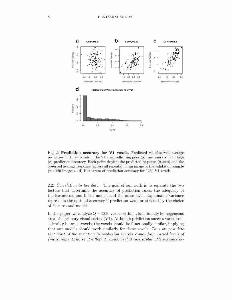
for image Ij and voxel r. Note that because f (r) was fitted on an independenttraining data set, it can be considered as fixed w.r.t. the validation sample.In Figure 2 we show examples of voxels with low, intermediate, and highprediction accuracies, and a histogram of accuracy for all 1250 voxels locatedwithin the V1 area. We can drop the superscript r because each voxel isanalyzed separately.

8 BENJAMINI AND YU

Fig 2: Prediction accuracy for V1 voxels. Predicted vs. observed averageresponses for three voxels in the V1 area, reflecting poor (a), medium (b), and high(c) prediction accuracy. Each point depicts the predicted response (x-axis) and theobserved average response (across all repeats) for an image of the validation sample(m=120 images). (d) Histogram of prediction accuracy for 1250 V1 voxels.

2.2. Correlation in the data. The goal of our work is to separate the twofactors that determine the accuracy of prediction rules: the adequacy ofthe feature set and linear model, and the noise level. Explainable variancerepresents the optimal accuracy if prediction was unrestricted by the choiceof features and model.

In this paper, we analyze Q = 1250 voxels within a functionally homogeneousarea, the primary visual cortex (V1). Although prediction success varies con-siderably between voxels, the voxels should be functionally similar, implyingthat our models should work similarly for these voxels. Thus we postulatethat most of the variation in prediction success comes from varied levels of(measurement) noise at different voxels; in that case explainable variance es-

SHUFFLE ESTIMATOR IN FMRI 9

timates should explain most of the voxel-to-voxel variability in prediction ac-curacy. Once the approach is validated on this controlled setting, explainablevariance can be used more broadly, for example to compare the predictabilitylevels of different functional areas.

Since we intend to use the validation sample with replicates to estimate theexplainable variances, we now give a few more details on how it was collected.Recall that the validation data consisted of m = 120 images each repeated n= 13 times (see Figure 3a). This data was recorded in 10 separate sessions,so that the subject could rest between sessions; the fMRI was re-calibratedat the beginning of each session. Each session contained all presentations of12 different images. A pseudo-random integer sequence ordered the repeatswithin a session3.

When we measure correlation across many voxels, we believe that the de-sign of the experiment induces strong correlation in the data. To see this,in Figure 3 (b-c) we plot the correlation between measurements at differenttime slots (each time slot is represented by the vector of Q=1250 measure-ments). This gives us a gross representation of the correlation for individualvoxels, including both noise driven and possibly stimuli-driven correlations.Clearly there are strong correlations between time-slots within a block, butno observable correlations between blocks. As these within-block correlationpatterns do not correspond to the stimuli schedule that is randomized withina block, we conclude the correlations are largely due to noise. These noisecorrelations need to be taken into account to correctly estimate the explain-able variance.

2.3. A probability model for the measurements. We introduce a probabilisticmodel for the measurements Y := (Yt)Tt=1 at a single voxel. Y is modeledas a random effects model with additive, correlated noise Williams [1952].Additivity of noise is considered a good approximation for fMRI event relateddesigns and is commonly used [Buracas and Boynton, 2002]. The randomeffects model accounts for the generalization of prediction accuracy fromthe validation sample to the larger population of natural images. In thissection the model is carefully developed based on the fMRI experiment, andthe quantities of interest for this model are defined in Section 2.4. Section2.5 introduces algebraic tools that will be used for developing the shuffleestimator.

Let {Ii}Mi=1 be the set of possible images from which we can sample. Weassume each possible Ii image has a fixed mean effect µi ∈ R relative to a

3The pseudo-random sequence allocated spots for 13 different images; no image wasshown in the last category and the responses were discarded.

10 BENJAMINI AND YU

Fig 3: Data acquisition for the validation data set. (a) The transposed designmatrix X � recording which image (y-axis) was displayed at each time slot t (x-axis).Data was recorded in blocks of 12 unique images repeated n = 13 times. (b-d)Temporal correlation, measured between a single time-point (t∗ = 40, 140, 240for b,c,d respectively), and all others points. The t = t∗ point is marked by bluevertical lines. On average, strong but non-smooth correlation are found within theblocks, but separate blocks seem uncorrelated. Note that we depict the aggregatecorrelation of all voxels here, but cannot from this infer the noise correlation ofany specific voxel. Furthermore, correlation depicted here is due to both noise andsignal.

grand mean on the fMRI response, with population quantities

1

M

M�

i=1

µi = 0,1

M

M�

i=1

µ2i = σ2

µ,

and we refer to σ2µ as the signal variance.

SHUFFLE ESTIMATOR IN FMRI 11

2.3.1. Random effects based on sampling. As discussed above, m inputs aresampled randomly from {Ii}Mi=1 (without replacement), denoted by the ran-dom function s : {1, ...,m} → {1, ...,M}. It will be useful to discuss thesampled mean effects directly. We denote Aj = µs(j) for j = 1, ...,m, ormarginally P(Aj = µi) = 1/M foreach i = 1, ...,M, j = 1, ...,m. We useA = (Aj)mj=1 for the random-effect column vector, and

A :=1

m

m�

j=1

Aj s2A :=1

(m− 1)

m�

j=1

(Aj − A)2

for the sample mean and sample variance of random effects. We assumeM is large, which is the case for our fMRI data; so Aj ’s are effectivelyindependent4. Then

EA[s2A] = σ2

µ

where EA is the expectation with respect to the sampling.

Images are shown in a long sequence (which may be composed of blocks) sothat each image is repeated multiple times. Our analysis will be conditionedon the schedule h(t) : {1, ..., T} → {1, ...m} defined earlier, so h(t) is regardedas fixed. h(t) can also be represented by fixed design matrix X ∈ RT×m, withXt,j = 1 if h(t) = j and 0 otherwise. To illustrate this, consider the followingtoy example (T = 5,m = 4):

h(1) = 1h(2) = 2h(3) = 3h(4) = 2h(5) = 3

⇐⇒ X ∈ RT×m =

1 0 0 00 1 0 00 0 1 00 1 0 00 0 1 0· · · ·

.

In this example, the second sampled image, or Is(2) is shown at time slots2 and 4. The (random) mean effect is represented by A2 = µs(2) in bothcases. (These are the first 5 rows in the design matrix used for the examplein Figure 4).

XX � ∈ RT×T marks repeats of the same stimulus so for t, u = 1, ..., T ,

(2.1) XX �t,u =

�1 if h(t) = h(u),0 otherwise.

2.3.2. Noise. We assume the components of the measurement noise vector� = (�t)Tt=1 are independent of the random treatment effects {Aj}mj=1, have0 mean, but may be correlated. The correlation captures the slow-changing

4Both the model and the shuffle estimator can be easily adapted for sampling from asmall library of images as well.

12 BENJAMINI AND YU

dynamics of hemodynamics and effects of preprocessing on fMRI signals.Hence,

(2.2) E�[�t] = 0; cov(�t, �u) = σ2�Σt,u Σt,t = 1,

or in matrix notation cov[�] = σ2�Σ for Σ ∈ RT×T .

2.3.3. Model for observed responses. We are now ready to introduce theobserved data (column) vector Y ∈ RT as follows:

(2.3) Y = XA+ �

and for single time slot tYt = Ah(t) + �t,

where {A1, ..., Am} are iid samples from {µ1, ..., µM}.

2.3.4. Response covariance. The model involves two independent sourcesof randomness:5 the image sampling modeled by random effects, and themeasurement errors, which are of unknown form.

Assuming independence between A and �, the covariance of Yt and Yu iscomposed of the covariance from the sampling and the covariance of thenoise,(2.4)covA,�(Yt, Yu) = covA(Ah(t), Ah(u)) + cov�(�t, �u) = σ2

µ1(h(t)=h(u)) + σ2�Σt,u.

The first term on the RHS shows that treatment (random) effects are un-correlated if they are based on different inputs, but are identical if based onthe same input, with a variance of σ2

µ. In matrix form, we get:

(2.5) EA,�[Y] = 0; covA,�(Y) = σ2µXX � + σ2

�Σ.

2.4. Explainable variance and variance components. We are ready to defineexplainable variance, the ratio of signal variance to total variance. Under un-correlated noise, explainable variance is identical to the interclass correlation.When noise is correlated, however, the two quantities diverge. Explainablevariance is relevent to the performance of prediction models, a property wewill discuss in Section 4.

5Throughout this paper, it is in fact enough to assume the responses are generatedaccording to E[Yt|A] = Ah(t) = µs(t) and cov(Yt, Yu|A) = σ2

�Σt,u without explicit addi-tivity.

SHUFFLE ESTIMATOR IN FMRI 13

Recall that Yj are the averaged responses per image (j = 1, ...,m for theimages in our sample), and let Y = 1

T

�Tt=1 Yt be the global average response.

Then the sample variance of averages is

(2.6) MSbet :=1

m− 1

m�

j=1

�Yj − Y

�2.

The notation MSbet refers to the mean-of-squares between treatments. Letus define the total variance σ2

Y as the population mean of MSbet,

(2.7) σ2Y := EA,�[MSbet].

Note that σ2Y is not strictly the variance of any particular Yj ; indeed, the

variance of Yj is not necessarily equal for different j’s6. Nevertheless, we willloosely use the term variance here and later, owing to the parallels betweenthese quantities and the variances in the iid noise case, which are furtherdiscussed in Section 4.

Yj is composed of a treatment part (Aj) and average noise part (�j); similarlyY is composed of A and �. By partitioning the MSbet and taking expectationsover the sampling and the noise we get

(2.8) EA,�[MSbet] = EA[1

m− 1

m�

j=1

�Aj − A

�2] + E�[

1

m− 1

m�

j=1

(�j − �)2],

where the cross-terms cancel because of the independence of the noise fromthe sampling. We can call the expectation of the second term the noise level,or σ2

� , and get the following decomposition

(2.9) σ2Y = σ2

µ + σ2�

In other words, the signal variance σ2µ and the noise level σ2

� are the signaland noise components of the total variance.

Finally, we define the proportion of explainable variance to be the ratio

ω2 := σ2µ/σ

2Y .

Explainable variance measures the proportion of variance due to treatmentin the averaged responses, hence is an alternative to signal-to-noise mea-sures.

Note that of the two expressions in ω2, σ2Y can be naturally estimated from

the sample, while σ2µ requires more work. To estimate σ2

µ the signal and noiseneed to be separated. As we see in the next section, one way to separate themis based on their different covariance structures.

6In practice, this is true for the individual measurements Yt as well. We chose Σt,t = 1for illustration reasons.

14 BENJAMINI AND YU

2.5. Quadratic contrasts. In this subsection we derive MSbet as a quadraticcontrast of the full data vector Y. This contrast would highlight the re-lation between σ2

Y or σ2� with both the design XX � and the measurement

correlations Σ, and would produce algebraic descriptions used in Section 3.These are simple extensions of classical treatment of variance components[Townsend and Searle, 1971].

Denote B := XX �/n, an RT×T scaled version of XX �, with

(2.10) Bt,u =

�1n if h(t) = h(u),0 otherwise.

B is an averaging matrix, meaning that multiplication of a measurementvector by B replaces each element in the vector by the treatment average,as in

(2.11) (BY)t = Yh(t).

It is easy to check that B = B� and B = B2. Also let G ∈ RT×T Gt,u = 1/Tfor t, u = 1, ..., T be the global average matrix, so that (GY)t = Y , t =1, ..., T . We can now express MSbet as a quadratic expression of Y

(2.12) MSbet =1

(m− 1)n�(B −G)Y�2.

or more generally as a function of any input vectorMSbet(·) := 1

(m−1)n�(B −G)(·)�2.

We derive the relation between total variance, the design, and the correlationof the noise.

σ2Y = EA,�[MSbet(Y)] = 1

(m−1)nEA,�[tr�(B −G)(Y�Y)(B −G)

�]

= 1(m−1)n tr ((B −G)covA,�(Y)(B −G)) .

The signal effect and noise are additive, hence

1(m−1)n tr ((B −G)covA(Y)) + 1

(m−1)n tr ((B −G)cov�(Y)) .

Substituting covA(Y) = nσ2µB and cov�(Y) = σ2

�Σ,

1(m−1)n tr

�(B −G)(nσ2

µB)�+ 1

(m−1)n tr�(B −G)σ2

�Σ�.

= 1(m−1)σ

2µtr(B −G) + 1

(m−1)nσ2� tr((B −G)Σ)

= σ2µ + 1

(m−1)nσ2� tr ((B −G)Σ) .

SHUFFLE ESTIMATOR IN FMRI 15

Derivation 1. Under the model described in Section 2.3,

(2.13) σ2Y = σ2

µ +1

(m− 1)nσ2� tr ((B −G)Σ)

As a direct consequence of (2.9,2.13) we get an exact expression for the noiselevel

(2.14) σ2� = 1

(m−1)nσ2� tr ((B −G)Σ) .

Obviously, σ2� scales with the noise variance of the individual measurements

σ2� . Moreover, σ2

� depends on the relation between the design and the mea-surement correlation Σ. Note that if there are no correlation within repeats,then tr ((B −G)Σ) = (m−1)σ2

� and σ2� = σ2

� /n. In that case σ2Y = σ2

µ+σ2� /n,

and by plugging in an estimator of σ2� , we can directly estimate σ2

� and σ2µ.

This gives us an estimator for ω2 if noise is uncorrelated

ω2 = 1− 1

F

for F the standard F statistic. This is method-of-moments estimator de-scribed fully in Section 6.1.

On the other hand, when some correlations within repeats are greater than0, σ2

� /n underestimates the level of the noise and inflates the explainablevariance. In the next section we introduce the shuffle estimators which candeal with correlated noise.

3. Shuffle estimators for signal and noise variances. In this sectionwe propose new estimators called the shuffle estimators for the signal andnoise level, and for the explainable variance. As in (2.9), σ2

Y = σ2µ + σ2

� , butthe noise variance σ2

� is a function of the (unknown) measurement correla-tion matrix Σ. Using shuffle estimators we can estimate σ2

µ and σ2� without

having to estimate the full Σ or imposing unrealistically strong conditionson it.

The key idea is to artificially create a second data vector that will havesimilar noise patterns as our original data (see Figure 4). We do this bypermuting, or shuffling, the original data with accordance to symmetries thatare based on the data collection. In Section 3.1 we formalize the definitionof such permutations that conserve the noise correlation and give plausibleexamples for neuroscience measurements. In Section 3.2 we compare thevariance of averages (MSbet) of the original data (Figure 4 b), with the same

16 BENJAMINI AND YU

contrast computed on the shuffled data (c). Because repeated measures forthe same image are shuffled into different categories, the variance due tosignal will be reduced in the shuffled data. We derive an unbiased estimatorfor signal variance σ2

µ based on this reduction in variance, and use the plug-inestimators for σ2

� and ω2.

Fig 4: Cartoon of the shuffle estimator. (a) Data is generated according toschedule h(t), with each color representing repeats of a different image. (b) Re-peats of each image are averaged together and the sample variance is computedon these averages. (c) Data is shuffled by P , in this example reversing the order.Now measurements which do not originate from the same repeat are averaged to-gether (Y ∗

j ’s), and the sample variance of the new averages is computed. Theseaverages should have a lower variance in expectation, and we can calculate thereduction amount α(h, P ) = 1

m−1 tr ((B −G)PBP �). (d) The shuffle estimator forsignal variance is the difference between the two sample variances, after correctionof 1− α(h, P ).

3.1. Noise conserving permutation for Y. A prerequisite for the shuffle es-timator is to find a permutation that will conserve the noise contribution toσ2Y . We will call such permutations noise-conserving w.r.t to h.

SHUFFLE ESTIMATOR IN FMRI 17

Recall (2.14),

σ2� =

1

(m− 1)ntr((B −G) (σ2

�Σ)),

where σ2�Σ = cov�[Y] as before. Let P ∈ RT×T be a permutation matrix.

Then

Definition 2. P is noise conserving w.r.t h, if

(3.1) tr�(B −G)Pσ2

�ΣP�� = tr

�(B −G)σ2

�Σ�.

Equivalently,

tr ((B −G) cov�[P ·Y]) = tr�(B −G)σ2

�Σ�.

Although we define the noise conserving property based on the covariance,replacing the covariance with the correlation matrix Σ would not change thepermutation class.

Noise conservation is a property that depends on the interplay betweenthe design B and the noise covariance Σ. Let us take a look at importantcases.

3.1.1. Trivial noise-conserving permutations. A permutation P that simplyrelabels the treatments is not a desirable permutation, even though it isnoise-conserving. We call such permutations trivial:

Definition 3. A permutation P , associated with permutation functiongP : {1...T} → {1...T}, is trivial if

(3.2) h(t) = h(u) ⇒ h(gP (t)) = h(gP (u)), ∀t, u.

It is easy to show that for trivial P , MSbet(PY) = MSbet(Y).

3.1.2. Noise conserving permutations based on symmetries of Σ. A usefulclass of non-trivial noise conserving permutations is the class of symmetriesin the correlation matrix Σ: a symmetry of Σ is a permutation P such thatPΣ = Σ. If P is a symmetry of Σ, then P is noise-conserving regardless ofthe design. Here are three important general classes of symmetries which arecommonly applicable in neuroscience.

1. Uncorrelated noise. The obvious example is the uncorrelated noisecase Σ = I where all responses are exchangeable. Hence any permuta-tion is noise-conserving.

18 BENJAMINI AND YU

2. Stationary time series Neuroscience data is typically recorded in along sequence containing a large number of serial recordings at constantrates. It is natural to assume that correlations between measurementswill depend on the time passed between the two measures, rather thanon the location of the pair within the sequence. We call this the station-ary time series. Under this model Σ is a Toeplitz matrix parameterizedby {ρd}T−1

d=0 , the set of correlation values Σt,u = ρd, where d = |t−u|.Though the correlation values ρd’s are related, this parameterizationdoes not enforce any structure on them. This robustness is important inthe fMRI data we analyze. For this model, a permutation that reversesthe measurement vector is noise conserving

(PY)t = YT+1−t.

This is the permutation we use on our data in Section 6.Another family of noise conserving permutations are the shift operator(PY)t = (Y)t+k (up to edge effects).

3. Independent blocks Another important case is when measurementsare collected in distinct sessions, or blocks. Measurements from dif-ferent blocks are assumed independent, but measurements within thesame block may be correlated, perhaps because of calibration of themeasurement equipment. We index the block assignment of time twith β(t). A simple parameterization for noise correlation would to letΣt,u = ζ(β(t),β(u)) depend only on the block identity of measurementst and u. We call this the block structure. Under the block structure,any permutation P (associated with function gP ) that maintains thesession structure, meaning

(3.3) β(t) = β(u) ⇒ β(gP (t)) = β(gP (u))

would be noise-conserving w.r.t. any h.

The scientist is given much freedom in choosing the permutation P , andshould consider both the variance of the estimator and the estimator’s ro-bustness against plausible noise-correlation structures. Establishing criteriafor choosing the permutation P is the topic of current research.

3.2. Shuffle estimators. We can now state the main results. From the follow-ing lemma we observe that every noise-conserving permutation establishesa mean-equation with two parameters: σ2

µ and σ2� . The coefficient for σ2

µ

is α(h, P ) := 1m−1 tr ((B −G)(PBP �)), which only depends on parameters

known to the scientist.

Lemma 4. If P is a noise-conserving permutation for Y, then

SHUFFLE ESTIMATOR IN FMRI 19

1. EA,�[MSbet(PY)] = α(h, P )σ2µ + σ2

� .

2. α(h, P ) ≤ 1, and the inequality is strict iff P is non-trivial.

Proof. 1. Using similar algebra as in Proposition 1, the expectationEA,�[MSbet(PY)] can be partitioned into a term depending on thesampling covariance covA(PY) and a term depending on the noisecovariance cov�(PY). Since P is noise-conserving, for the noise term:

cov�(PY) = σ2� .

As for the sampling:

covA(PY) = PcovA(Y)P � = σ2µP (nB)P �.

Hence,1

(m−1)nσ2µtr

�(B −G)(P (nB)P �)

�= α(h, P )σ2

µ.

2. In Proposition 1 we saw that the sampling component for the unper-muted vector covA(Y) is σ2

µ. Hence for P the identity matrix I ∈ RT×T

we have α(I, h) = 1. For all other P ’s, note that the global meanterm (G) is unaffected by the permutation (PG = G) or the averaging(BG = G), so it remains unchanged.

From the Cauchy-Schwartz inequality,

tr�B(PBP �)

�≤ tr (BB) = tr(B)

as P is unitary and B a projection Recall that P is trivial if P reordersmeasurements within categories and renames categories. It is easy tocheck that PBP � = B iff P is trivial. For trivial P ’s, we again getequations similar to Proposition 1, so α(P, h) = 1.For any non-trivial permutation B �= PBP �, in which case the CS-inequality is strict resulting in α(h, P ) < 1.

As can be seen in the proof, α depends only on B and P which are bothknown:

(3.4) α(h, P ) = 1m−1 tr

�(B −G)(PBP �)

�

It reflects how well P "mixes" the treatments; the greater the mix, the smallerα.

20 BENJAMINI AND YU

The consequence of the second part of the lemma is that for any non-trivialP , we get a mean-equation which is linearly independent from the equa-tion based on the original data (because α(h, P ) < 1). In other words, theequation set

(3.5)�

EA,�[MSbet(Y)] = σ2µ + σ2

�

EA,�[MSbet(PY)] = α(h, P )σ2µ + σ2

�

can be solved.

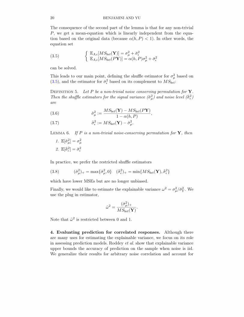
This leads to our main point, defining the shuffle estimator for σ2µ based on

(3.5), and the estimator for σ2� based on its complement to MSbet:

Definition 5. Let P be a non-trivial noise conserving permutation for Y.Then the shuffle estimators for the signal variance (σ2

µ) and noise level (ˆσ2� )

are

σ2µ :=

MSbet(Y)−MSbet(PY)

1− α(h, P ),(3.6)

ˆσ2� := MSbet(Y)− σ2

µ.(3.7)

Lemma 6. If P is a non-trivial noise-conserving permutation for Y, then

1. E[σ2µ] = σ2

µ

2. E[ˆσ2� ] = σ2

�

In practice, we prefer the restricted shuffle estimators

(3.8) (σ2µ)+ = max{σ2

µ, 0} (ˆσ2� )+ = min{MSbet(Y), ˆσ2

� }

which have lower MSEs but are no longer unbiased.

Finally, we would like to estimate the explainable variance ω2 = σ2µ/σ

2Y . We

use the plug in estimator,

ω2 =(σ2

µ)+MSbet(Y)

.

Note that ω2 is restricted between 0 and 1.

4. Evaluating prediction for correlated responses. Although thereare many uses for estimating the explainable variance, we focus on its rolein assessing prediction models. Roddey et al. show that explainable varianceupper bounds the accuracy of prediction on the sample when noise is iid.We generalize their results for arbitrary noise correlation and account for

SHUFFLE ESTIMATOR IN FMRI 21

generalization from sample to population7. As shown in Lemma 7, the noiselevel σ2

� is the optimal expected loss under mean square prediction error(MSPE) loss, and the explainable variance ω2 approximates the accuracyunder squared-correlation Corr2 utility.

First let us recall the setup. Let f be a prediction function that predicts areal-valued response to any possible image (out of a population of M):

(4.1) f : {Ii}Mi=1 → R.

We will assume f does not depend on the sample we are evaluating, meaningthat it was fit on separate data. We usually think of f as using some aspectsof the image to predict the response, although we do not restrict it in anyparametric way to the image.

Prediction accuracy is measured only on the m images sampled for the (non-overlapping) validation set. Recall s : {1, ...,m} → {1, ...,M} is the ran-dom sampling function. For the j’th sampled image, the predicted responsef(Is(j)) is compared with the average observed response for that image Yj .We consider two common accuracy measures: mean squared prediction error(MSPE[f ]) and the squared correlation (Corr2[f ]), defined

MSPE[f ] :=1

m− 1

m�

j=1

�f(Is(j))− Yj

�2,

(4.2)

Corr2[f ] :=Corr2j (f(Is(j)), Yj) =

�1

m−1

�mj=1(f(Is(j))− fs)(Yj − Y )

�2

1m−1

�mj=1(f(Is(j))− fs)2

�mj=1(Yj − Y )2

,

(4.3)

where fs denotes the average of the predictions for the sample.

We will state and discuss the results relating the explainable variance tooptimal prediction; details can be found in the appendix.

Lemma 7. Let f∗ : {Ii}Mi=1 → R be the prediction function that assigns foreach stimulus Ii its mean effect µi, or f∗(Ii) = µi. Under the model describedin Section 2.3,

(a) f∗ = argminf EA,�[MSPE[f ]];

(b) σ2� = EA,�[MSPE[f∗]] = minf EA,�[MSPE[f ]];

7While these results may have been proved before, we have not found them discussedin similar context.

22 BENJAMINI AND YU

(c) ω2 ≈ EA,�[Corr2[f∗]] with a bias term smaller than 1m−1 .

Under our random effects model, the best prediction (in MSPE) is obtainedby the mean effects, or f∗. More important to us, the accuracy measuresassociated with the optimal prediction f∗ can be approximated by signaland noise levels: σ2

� for MSPE[f∗] and ω2 for Corr2[f∗].

The main consequence of this lemma is that the researcher does not need a"good" prediction function to estimate the "predictability" of the response.Prediction is upper-bounded by ω2, a quantity which can be estimated with-out setting a specific function in mind. Moreover, when a researcher doeswant to evaluate a particular prediction function f , ω2 can serve as a yardstick with which f can be compared. If Corr2[f ] ≈ ω2, the prediction erroris mostly because of variability in the measurement. Then the best way toimprove prediction is to reduce the noise by preprocessing or by increasingthe number of repeats. On the other hand, if Corr2[f ] � ω2, there is stillroom for improvement of the prediction function f .

5. Simulation. We simulate data with a noise component generated fromeither a block structure or a times-series structure, and compute shuffle es-timates for signal variance and for explainable variance. For a wide rangeof signal-to-noise regimes, our method produces unbiased estimators of σ2

µ.These estimators are fairly accurate for sample sizes resembling our image-fMRI data, and the bias in the explainable variance ω2 is small compared tothe inherent variability. These results are shown in Figure 5. In Figure 6 weshow that under non-zero σ2

µ, the shuffle estimates have less bias and lowerspread compared to the parametric model using the correctly specified noisecorrelation.

5.1. Block structure. For the block structure we assumed the noise is com-posed of an additive random block effect constant within blocks (bk, k =1, ..., B blocks), and an iid Gaussian term (et, t = 1, ..., T )

Yt = A(t) + bβ(t) + et

Aj , bk and et are sampled from centered normal distributions with variances(σ2

µ,σ2b ,σ

2e). We used σ2

b = 0.5,σ2e = 0.7, and varied the signal level σ2

µ =0, 0.1, ..., 0.9. We used m = 120, n = 15, with all presentations of every 5stimuli composing a blocks (B = 20 blocks). For each of these scenarios weran 1000 simulations, sampling the signal, block, and error effects. MSbet

was estimated the usual way, and P was chosen to be a random permutationwithin each block (α(h, P ) = 0.115). The results are shown in Figure 5 (a).

SHUFFLE ESTIMATOR IN FMRI 23

Fig 5: Simulations for the block and time-series (a) Simulation results com-paring shuffle estimates for signal variance σ2

µ (black) and explainable variance ω2

(blue) to the true population values (dashed line). Noise correlation followed an in-dependent block structure: noise within blocks was correlated, and between blockswas independent. The x-axis represents the true signal variance σ2

µ of the data, andthe y-axis marks the average of the estimates and [0.25,0.75] quantile range. (b)Similar plot for data generated under a stationary time-series model.

5.2. Time-series Model. For the time-series model we assumed the noisevector e ∈ RT is distributed as a multivariate Gaussian with mean 0 and acovariance matrix Σ, where Σ is an exponentially decaying covariance witha nugget,

Σt,u = ρ|t−u| = λ1 · exp{−|t− u|/λ2}+ (1− λ1)1(t=u).

Then Y = A(t) + et with the random effects A(t) sampled from N (0,σ2µ) for

σ2µ = 0, 0.1, ...0.9. We used m = 120, n = 15, and the parameters for the

noise were λ1 = 0.7 and λ2 = 30, meaning ρ125 ≈ 0.01. The schedule oftreatments was generated randomly. For each of these scenarios we ran 1000simulations, sampling the signal and the noise. In Figure 5 (b) we estimatedthe shuffle estimator with P the reverse permutation (gP (t) = T + 1 − t),resulting in α(h, P ) = 0.064.

5.3. Comparison to REML. In Figure 6 we used time-series data to compareσ2µ estimates based on the shuffle estimators to those obtained by an REML

24 BENJAMINI AND YU

Fig 6: Comparison of methods on simulation. Each pair of box-plots repre-sents the estimated signal variance σ2

µ using the shuffle estimator (dark gray) andREML (light gray) for 1000 simulations. The blue horizontal line represents thetrue value of σ2

µ. The REML estimator assumes the correct model for the noise,while the shuffle estimator only assumes a stationary time series. When there is nosignal, REML outperforms the shuffle estimators, but in all other cases it is bothbiased and has greater spread.

estimator with the correct parametrization for the noise correlation matrix.We used nlme package in R to fit a repeated measure analysis of variancefor the exponentially decaying correlation of noise with a nugget effect. Thecomparison included 1000 simulations for σ2

µ = 0, 0.2, 0.4, 0.6, 0.8, and a noisemodel identical to Section 5.2.

5.4. Results. Figure 5 describes the performance of shuffle estimates on twodifferent scenarios: block correlated noise (a), and stationary time-series noise(b). For signal variance (black) the shuffle estimator gives unbiased estimates.The shuffle estimator for explainable variance is not unbiased, but the biasis negligible compared to the variability in the estimates. In Figure 6, wecompare the signal variance estimates based on the shuffle estimator (darkgray) with estimates based on REML (light gray). The estimates based onthe shuffle have no bias, while those based on REML underestimate thesignal. The variance of the REML estimates is slightly larger, due in partare slightly better in both bias and in variance.

SHUFFLE ESTIMATOR IN FMRI 25

6. Data. We are now ready to evaluate prediction models using the shuf-fle estimates for explainable variance. Prediction accuracy was measured forencoding models of 1250 voxels within the primary visual cortex (V1). Be-cause V 1 is functionally homogenous, encoding models for voxels within thiscortical area should work similarly. As observed in Figure 2, there is largevariation between prediction accuracies for the different voxels. We postulatethat most of the variation in prediction accuracy would come from variedlevels of noise at different voxels; in that case good explainable variance es-timates should explain most of the voxel-to-voxel variability in predictionaccuracy.

Prediction accuracy values for these 1250 voxels are compared to explainablevariance estimates for each voxel, as generated by the shuffle estimator. Wealso compare the accuracy values to alternative estimates for explainablevariance, using the method of moments for uncorrelated noise, and REMLunder several parameterizations for the noise:

6.1. Methods. Several methods are compared for estimating the explainablevariance (ω2 = σ2

µ/σ2Y ). The methods differ in how σ2

µ is estimated; allmethods use the sample averages variance MSbet(Y) for σ2

Y , and plug inthe two estimates into ω2. We estimate ω2 separately for each voxel (r =1, ..., 1250). The methods we compare are

1. The shuffle estimators estimator. We assume time-series stationaritywithin each block, and independence between the blocks, so choose aP that reverses the order of the measurements, (PY)t = YT+1−t).Because the size of the blocks is identical, reversing the order of thedata vector is equivalent to reversing the order within each block.α(h, P ) = 0.17. We use the restricted estimator

(σ2µ)+ = max

�MSbet(Y)−MSbet(PY)

1− α(h, P ), 0

�

for signal variance, and the explainable variance is obtained by pluggingthe estimate of σ2

µ into ω2 = σ2µ/MSbet.

2. An estimator (ω2) unadjusted for correlation. We use the mean-squarewithin (MSwit =

1(m−1)n

�mj=1

�t:h(t)=j(Yt−Yj)2) contrast to estimate

the noise variance σ2� , scale by 1/n to estimate the noise level σ2

� ,and remove the scaled estimate from MSbet, σ2

µ = MSbet −MSwit/n.Explainable variance is obtained by plug in estimator ω2 = σ2

µ/MSbet.

3. Estimators based on a parametric noise model.

• We assume the noise is generated from an exponentially decayingcorrelation matrix, with a nugget effect. This means Ct,t+d =

26 BENJAMINI AND YU

λ2exp(−d/λ1) + 1(d=0)(1 − λ2) where the rate of decay λ1 andnugget effect λ2 where additional parameters. If λ2 = 0, this isequivalent to the AR(1) model.

• Alternatively, we assume the noise is generated from an AR(3)process, or �t = ηt +

�3k=1 ak�t−k. This models allows for non-

monotone correlations.

We use the nlme package in R to estimate the signal variance of thismodel using restricted maximum likelihood (REML, e.g. Laird et al.[1987]), and use the plug-in estimator for the explainable variance.

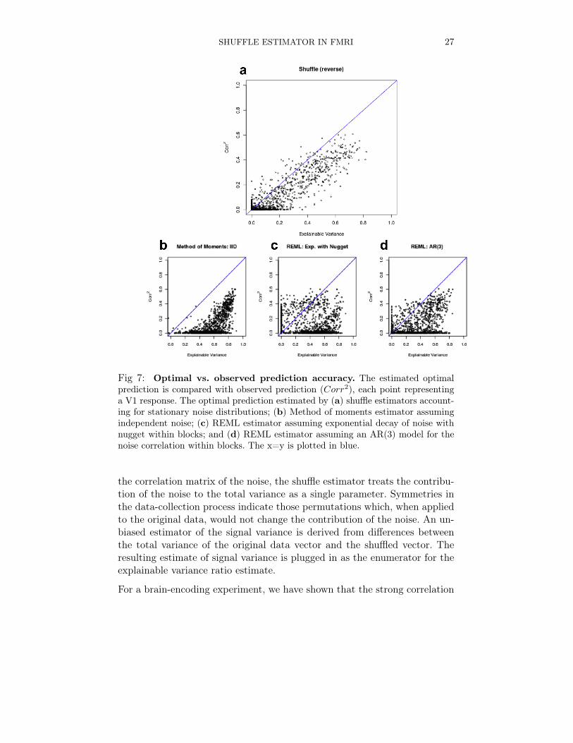
6.2. Results. In Figure 7 we compare the prediction accuracy of the vox-els to estimates of the explainable variance. Each panel has 1250 pointsrepresenting the 1250 voxels: the x coordinate is the estimate of explain-able variance for the voxel, and the y coordinate is Corr2[f ] for the Ga-bor based prediction-rule. The large panel shows the shuffle estimators forexplainable variance. The relation between Corr2[f ] and ω2 is very linear(r = 0.9). Almost all voxels for which accuracy is close to random guess-ing (Corr2[f ] < 0.05) could be identified based on low explainable variancewithout knowledge of the specific feature set. Although there is still roomfor improving prediction for some voxels, the Gabor models are not far fromperforming optimally on these recordings.

When we try to repeat this analysis with other ω2 estimators, explainablevariance estimates are no longer strongly related with the prediction accu-racy. When correlation in the noise is ignored (b), signal strength is greatlyoverestimated. In particular, some of the voxels for which prediction accu-racy is almost 0 have very high estimates of explainable variance (as highas ω2 = 0.8). In contrast to the shuffle estimates, it is hard to learn fromthese explainable variance estimates about the prediction accuracy for avoxel.

This incompatibility of prediction accuracy and explainable variance esti-mates is also observed when the estimates are based on maximum likelihoodmethods that parameterize the noise matrix. For the AR(3) model in (d), wesee variability between explainable variance estimates for voxels with givenprediction accuracy level. The smaller model (c) seems to suffer from bothoverestimation of signal and high variance.

7. Discussion. We have presented the shuffle estimator, a resampling-based estimator for the explainable variance in a random-effects additivemodel with auto-correlated noise. Rather than parameterize and estimate

SHUFFLE ESTIMATOR IN FMRI 27

Fig 7: Optimal vs. observed prediction accuracy. The estimated optimalprediction is compared with observed prediction (Corr2), each point representinga V1 response. The optimal prediction estimated by (a) shuffle estimators account-ing for stationary noise distributions; (b) Method of moments estimator assumingindependent noise; (c) REML estimator assuming exponential decay of noise withnugget within blocks; and (d) REML estimator assuming an AR(3) model for thenoise correlation within blocks. The x=y is plotted in blue.

the correlation matrix of the noise, the shuffle estimator treats the contribu-tion of the noise to the total variance as a single parameter. Symmetries inthe data-collection process indicate those permutations which, when appliedto the original data, would not change the contribution of the noise. An un-biased estimator of the signal variance is derived from differences betweenthe total variance of the original data vector and the shuffled vector. Theresulting estimate of signal variance is plugged in as the enumerator for theexplainable variance ratio estimate.

For a brain-encoding experiment, we have shown that the strong correlation

28 BENJAMINI AND YU

present in the fMRI measurements greatly compromises classical methodsfor estimating explainable variance. We used prediction accuracy measuresof a well-established parametric model for voxels in the primary visual cor-tex as indicators of the explainable signal variance at each of the voxels.Shuffle estimates of the explainable variance explained most of the variationbetween voxels, even though they were blind to features of the image. Othermethods did not do well: methods that ignored noise correlation seem togreatly overestimate the explainable variance, while methods that estimatedthe full correlation matrix were considerably less informative with regardsto prediction accuracy. We consider this convincing evidence that the shuf-fle estimators for explainable variance can be used reliably even when nogold-standard prediction model is present.

Explainable variance is an assumption-less measure of signal, in that it makesno assumptions about the structure of the mean function that relates the in-put image to response. We find it attractive that the shuffle estimator forexplainable variance similarly requires only weak assumptions for the cor-relation of the noise. This makes the shuffle estimator a robust tool, whichcan used at different stages of the processing of an experiment: from opti-mizing of the experimental protocol, through choosing the feature space forthe prediction models, to fitting the prediction models.

The shuffle estimators may be useful for applications outside of neuroscience.These estimators can be used to estimate the variance associated with thetreatments of an experiment, conditioned on the design, whenever measure-ment noise is correlated. Spatial correlation in measurements arise in manydifferent domains, from agricultural experiments to DNA microarray chips.Shuffle estimators could provide an alternative to parametric fitting of thenoise contributions for these applications.

Future research should be directed at expressing the variance of the shuffleestimator for a candidate permutation, as well as at developing optimal waysto combine information from multiple noise conserving permutations. Moregenerally, shuffle estimators are a single example of adapting relatively newnon-parametric approaches from hypothesis testing into estimation; we seemuch room for expanding the use of permutation methods for creating robustestimators for experimental settings.

8. Acknowledgements. We are grateful to An Vu and members of JackGallant’s laboratory for access to the data and models and for helpful discus-sions about the method, and to Terry Speed and Philip Stark for suggestionsthat greatly contributed to this work. We are also thankful to two anony-mous reviewers and two editors whose insightful comments helped improvethis manuscript.

SHUFFLE ESTIMATOR IN FMRI 29

References.

Giedrius T. Buracas and Geoffrey M. Boynton. Efficient design of event-related fmri exper-iments using m-sequences. NeuroImage, 16(3, Part A):801 – 813, 2002. ISSN 1053-8119.. URL http://www.sciencedirect.com/science/article/pii/S105381190291116X.

Matteo Carandini, Jonathan B. Demb, Valerio Mante, David J. Tolhurst, Yang Dan,Bruno A. Olshausen, Jack L. Gallant, and Nicole C. Rust. Do We Know What theEarly Visual System Does? The Journal of Neuroscience, 25(46):10577 –10597, 2005. .URL http://www.jneurosci.org/content/25/46/10577.abstract.

P. Dayan, L.F. Abbott, and L. Abbott. Theoretical neuroscience: Computational and

mathematical modeling of neural systems. The MIT Press, 2001.E.S. Edgington and P. Onghena. Randomization tests, volume 191. CRC Press, 2007.Michael D. Fox and Marcus E. Raichle. Spontaneous fluctuations in brain activity observed

with functional magnetic resonance imaging. Nat Rev Neurosci, 8(9):700–711, 2007.ISSN 1471-003X. . URL http://dx.doi.org/10.1038/nrn2201.

R. Haefner and B. Cumming. An improved estimator of Variance Explained in the presenceof noise. Advances in neural information processing systems, pages 1–8, 2008.

A. Hsu, A. Borst, and F. E Theunissen. Quantifying variability in neural responses andits application for the validation of model predictions. Network: Computation in Neural

Systems, 15(2):91–109, 2004.S. A. Huettel. Event-related fMRI in cognition. NeuroImage, (0):–, 2011. . URL http:

//www.sciencedirect.com/science/article/pii/S1053811911010639.O. Josephs, R. Turner, and K. Friston. Event-related fMRI. Human brain mapping, 5(4):

243–248, 1997.K. N Kay, T. Naselaris, R. J Prenger, and J. L Gallant. Identifying natural images from

human brain activity. Nature, 452(7185):352–355, 2008.Nan Laird, Nicholas Lange, and Daniel Stram. Maximum Likelihood Computations

with Repeated Measures: Application of the EM Algorithm. Journal of the Amer-

ican Statistical Association, 82(397):97–105, 1987. ISSN 0162-1459. . URL http:

//www.jstor.org/stable/2289129.T. Naselaris, R. J Prenger, K. N Kay, M. Oliver, and J. L Gallant. Bayesian reconstruction

of natural images from human brain activity. Neuron, 63(6):902–915, 2009.S. Nishimoto, A.T. Vu, T. Naselaris, Y. Benjamini, B. Yu, and J.L. Gallant. Reconstructing

Visual Experiences from Brain Activity Evoked by Natural Movies. Current Biology,2011.

Brian N. Pasley, Stephen V. David, Nima Mesgarani, Adeen Flinker, Shihab A. Shamma,Nathan E. Crone, Robert T. Knight, and Edward F. Chang. Reconstructing speechfrom human auditory cortex. PLoS Biol, 10(1):e1001251, 2012. . URL http://dx.doi.

org/10.1371%2Fjournal.pbio.1001251.A. Pasupathy and C.E. Connor. Responses to contour features in macaque area V4.

Journal of Neurophysiology, 82(5):2490, 1999.Francisco Pereira, Greg Detre, and Matthew Botvinick. Generating text from functional

brain images. Frontiers in Human Neuroscience, 5(00072):0, 2011. ISSN 1662-5161.. URL http://www.frontiersin.org/Journal/Abstract.aspx?s=537&name=human_

neuroscience&ART_DOI=10.3389/fnhum.2011.00072.J C Roddey, B Girish, and J P Miller. Assessing the performance of neural encoding

models in the presence of noise. Journal of Computational Neuroscience, 8(2):95–112,2000. ISSN 0929-5313. URL http://www.ncbi.nlm.nih.gov/pubmed/10798596. PMID:10798596.

M. Sahani and J. F Linden. How linear are auditory cortical responses? Advances in

neural information processing systems, pages 125–132, 2003.H. Scheffe. The analysis of variance, volume 72. Wiley-Interscience, 1959.

30 BENJAMINI AND YU

S. Shoham, L. M Paninski, M. R Fellows, N. G Hatsopoulos, J. P Donoghue, and R. ANormann. Statistical encoding model for a primary motor cortical brain-machine in-terface. IEEE Transactions on Biomedical Engineering, 52(7):1312–1322, 2005. ISSN0018-9294. .

E. C Townsend and S. R Searle. Best quadratic unbiased estimation of variance com-ponents from unbalanced data in the 1-way classification. Biometrics, pages 643–657,1971.

V.Q. Vu, P. Ravikumar, T. Naselaris, K.N. Kay, J.L. Gallant, and B. Yu. Encoding anddecoding V1 fMRI responses to natural images with sparse nonparametric models. The

Annals of Applied Statistics, 5(2B):1159–1182, 2011.Edward Vul, Christine Harris, Piotr Winkielman, and Harold Pashler. Puzzlingly high

correlations in fmri studies of emotion, personality, and social cognition. Perspectives on

Psychological Science, 4(3):274–290, 2009. . URL http://pps.sagepub.com/content/

4/3/274.abstract.R. M. Williams. Experimental Designs for Serially Correlated Observations. Biometrika,

39(1/2):151–167, 1952. ISSN 0006-3444. . URL http://www.jstor.org/stable/

2332474.M.W. Woolrich, B.D. Ripley, M. Brady, and S.M. Smith. Temporal autocorrelation in

univariate linear modeling of FMRI data. Neuroimage, 14(6):1370–1386, 2001.

9. Appendix.

9.1. Lemma (7). Let f∗ : {Ii}Mi=1 → R be the prediction function thatassigns for each stimulus Ii its mean effect µi, or f∗(Ii) = µi. Under theexperimental conditions and model described above,

(a) f∗ = argminf EA,�[MSPE[f ]];

(b) σ2� = EA,�[MSPE[f∗]] = minf EA,�[MSPE[f ]];

(c) ω2 ≈ EA,�[Corr2[f∗]] with a bias term smaller than 1m−1 .

Proof. (a) + (b)First, for any image in the sample, we compare the prediction with theexpected average given the sampling,

(9.1) MSPE[f ] =1

m− 1

m�

j

�(f(Is(j))− E�[Yj ]) + (E�[Yj ]− Yj)

�2.

From our model, E�[Yj ] = Aj . Substituting this into 9.1 and taking expecta-tion over the noise, we get

E�[MSPE[f ]] =1

m− 1[E�

m�

j

�f(Is(j))−Aj

�2+ E�

m�

j

�Aj − Yj

�2

+ E�

m�

j

(f(Is(j))−Aj)�Aj − Yj

�].

SHUFFLE ESTIMATOR IN FMRI 31

Recall that Yj − Aj is �j for each j, with E�[�j ] = 0 and a sample varianceσ2� . Therefore

(9.2) E�[MSPE[f ]] =1

m− 1[m�

j

�f(Is(j) −Aj

�2] + σ2

� .

By also taking an expectation over the sampling

(9.3) E[MSPE[f ]] = EAE�[MSPE[f ]] =m

m− 1

1

M

M�

i

[(f(Ii)− µi)2]+ σ2

� .

Proof. (c)Since the optimal f∗ maps each image Ii to its mean-effect µi, for the sampledimage it maps the random effect:

f∗(Is(j)) = µs(j) = Aj .

Hence Corr2[f∗] = Corr2j (Aj , Yj), or in extended form

(9.4) Corr2j (Aj , Yj) =

�1

m−1

�mj=1(Aj − A)(Yj − Y )

�2

�1

m−1

�mj=1(Aj − A)2

��1

m−1

�mj=1(Yj − Y )2

� .

Recall that Yj = Aj + �j . Equation (9.4) becomes

(9.5)

�1

m−1

�mj=1

�(Aj − A)(Aj − A) + (Aj − A)(�j − �)

��2

�1

m−1

�mj=1(Aj − A)2

��1

m−1

�mj=1(Yj − Y )2

� .

Let

s2A = 1m−1

m�

j=1

(Aj − A)2; s2� =1

m−1

m�

j=1

(Aj − A)2; MSbet =1

m−1

m�

j=1

(Yj − Y )2;

represent the sample variance of the treatment effects, averaged noise, andaverage measurements respectively. Moreover, let

r =

�mj=1(Aj − A)(�j − �)

(m− 1) sA · s�

be the empirical correlation of the treatment effects and the averaged noise.

32 BENJAMINI AND YU

Substituting into Equation 9.5 results in:�s2A + sA s� r

�2

s2AMSbet=

s2A + 2sA s� r + s2� r2

MSbet.

By taking expectations over A and � and approximating the expectations ofthe ratio with the ratio of the expectations, we get:

EA,�[Corr2[f∗]] =EA,�

�s2A + 2sA s� r + s2� r2

MSbet

�

=EA,�

�s2A

MSbet

�+ EA,�

�2sA s� r + s2� r2

MSbet

�

≈EA,�

�s2A

�

EA,� [MSbet]+

EA,��2sA s� r + s2� r2

�

EA,� [MSbet]

= ω2 +EA,�

�2sA s� r] + s2� r2

�

σ2Y

Since the mean effects Aj ’s and averaged noise �j ’s are independent, E[r] = 0.Hence

EA,�[Corr2[f∗]] ≈ ω2 + σ2�

E�r2�

σ2Y

.

Under mild conditions and m large enough√m− 1 rA,� ≈ N (0, 1). We get

a bias on the order of σ2�

σ2Y

1m−1 < 1

m−1 . Note that unless σ2µ/σ

2Y ≈ 0, the bias

is negligible compared to the deviation of 2sA s� rMSbet

which is of order 1√m−1

.

Yuval BenjaminiDepartment of StatisticsE-mail: yuvalb@stat.berkeley.edu

Bin YuDepartment of StatisticsE-mail: binyu@stat.berkeley.edu