the signomial global optimization algorithm some …users.abo.fi/alundell/files/euroxxiv.pdf · the...
TRANSCRIPT
The Signomial Global Optimization
Algorithm – Some Recent Advances
Andreas Lundell and Tapio Westerlund
Center of Excellence in Optimization and Systems EngineeringProcess Design & Systems EngineeringÅbo Akademi University, Finland
24th European Conference on Operations Research – EURO XXIV
July 11–14, Lisbon, Portugal

Introduction 2 | 18
The signomial global optimization algorithm
I Is a global optimization algorithm for solving MINLP problemscontaining signomial functions to global optimality.
I Convex underestimators for signomial functions throughsingle-variable transformations xi = T ji (X ji ) applied termwise.
. Transformations obtained by solving a MILP problem.
. Piecewise linear functions (PLFs) are used to approximateT ji (X ji ).
⇒ Gives a convex overestimation of the feasible region.
I The overestimated convex MINLP problem is solved using anyconvex solver.
I As the PLFs are updated, the approximations are improved.
Introduction 3 | 18
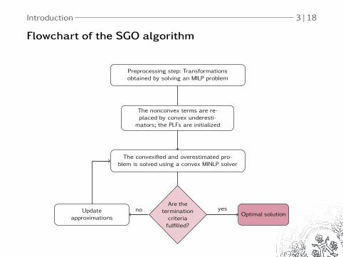
Flowchart of the SGO algorithm
Preprocessing step: Transformationsobtained by solving an MILP problem
The nonconvex terms are re-placed by convex underesti-
mators; the PLFs are initialized
The convexified and overestimated pro-blem is solved using a convex MINLP solver
Are thetermination
criteriafulfilled?
Updateapproximations
Optimal solutionno yes

Introduction 4 | 18
The considered class of MINLP problems
The mixed integer signomial programming (MISP) problem
formulation
minimize f(x) x= (x1,x2, . . . ,xI )
subject to Ax= a Bx ≤ bgn(x) ≤ 0 n = 1,2, . . . ,Jnqm(x)+ σm(x) ≤ 0 m = 1,2, . . . ,Jm
I The vector x can contain both continuous and integer-valuedvariables.
I The differentiable real functions f and g are (pseudo)convex,and the functions q and σ are convex and signomialrespectively.

Introduction 5 | 18
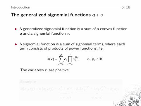
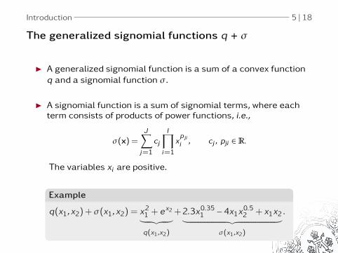
The generalized signomial functions q + σ
I A generalized signomial function is a sum of a convex functionq and a signomial function σ .
I A signomial function is a sum of signomial terms, where eachterm consists of products of power functions, i.e.,
σ(x) =J∑
j=1
cj
I∏i=1
xp jii , cj , pji ∈R.
The variables xi are positive.
Example
q(x1,x2)+ σ(x1,x2) = x21 + ex2︸ ︷︷ ︸q(x1,x2)
+2.3x0.351 −4x1x
0.52 + x1x2︸ ︷︷ ︸
σ(x1,x2)
.
Introduction 5 | 18
The generalized signomial functions q + σ
I A generalized signomial function is a sum of a convex functionq and a signomial function σ .
I A signomial function is a sum of signomial terms, where eachterm consists of products of power functions, i.e.,
σ(x) =J∑
j=1
cj
I∏i=1
xp jii , cj , pji ∈R.
The variables xi are positive.
Example
q(x1,x2)+ σ(x1,x2) = x21 + ex2︸ ︷︷ ︸q(x1,x2)
+2.3x0.351 −4x1x
0.52 + x1x2︸ ︷︷ ︸
σ(x1,x2)
.

The transformation approach 6 | 18
Convexification and relaxation of MISP problems
1. Convexification
I Every signomial term can be transformed to convex form byusing single variable transformations.
I In the process, additional variables and a number of nonlinearequality constraints defining the inverse transformations areobtained.
2. Underestimation, convexification and relaxation
I By using properly selected transformations, the convexifiedterms are underestimated when the inverse transformationsare approximated by piecewise linear functions.
I The MINLP problem is now convexified and relaxed.

The transformation approach 7 | 18
Transformation of the signomial constraints
qm(x)+ σm(x) ≤ 0
qm(x)+ σCm(x,X) ≤ 0
1.
qm(x)+ σCm(x,X̂) ≤ 0
2.
1. Convexification of σm by transformations xi = T ji (X ji ).Nonconvexities moved to Xji = T−1
ji (xi ).
2. Underestimation of σCm by approximating X ji = T ji
−1(xi )with PLFs X̂ ji . The integer-relaxed problem is now convexand overestimates the original problem.

The transformation approach 8 | 18
Convexifying nonconvex signomial terms
I Positive signomial terms can be convexified by. power transformations (PPT, NPT), xi = X ji
Q ji
. exponential transformation (ET), xi = eX ji
I Negative signomial terms can be convexified by. power transformations (PT), xi = X ji
Q ji
I A set of transformations for the nonconvex signomialterms is found by solving an MILP problem.
I The transformation sets are optimal w.r.t. certain strategyparameters. For example:. The number of transformations required is minimal.. The number of variables transformed is minimal.

The transformation approach 9 | 18
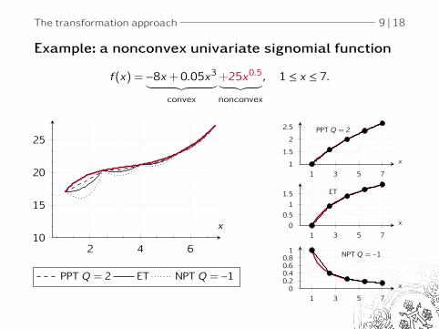
Example: a nonconvex univariate signomial function
f(x) = −8x +0.05x3︸ ︷︷ ︸convex
+25x0.5︸ ︷︷ ︸nonconvex
, 1 ≤ x ≤ 7.
2 4 610
15
20
25
x
PPT Q = 2 ET NPT Q = −1
1 3 5 71
1.5
2
2.5
x
PPT Q = 2
1 3 5 70
0.51
1.5
x
ET
1 3 5 70
0.20.40.60.8
1
x
NPT Q = −1

The transformation approach 9 | 18
Example: a nonconvex univariate signomial function
f(x) = −8x +0.05x3︸ ︷︷ ︸convex
+25x0.5︸ ︷︷ ︸nonconvex
, 1 ≤ x ≤ 7.
2 4 610
15
20
25
x
PPT Q = 2 ET NPT Q = −1
1 3 5 71
1.5
2
2.5
x
PPT Q = 2
1 3 5 70
0.51
1.5
x
ET
1 3 5 70
0.20.40.60.8
1
x
NPT Q = −1
The transformation approach 9 | 18
Example: a nonconvex univariate signomial function
f(x) = −8x +0.05x3︸ ︷︷ ︸convex
+25x0.5︸ ︷︷ ︸nonconvex
, 1 ≤ x ≤ 7.
2 4 610
15
20
25
x
PPT Q = 2 ET NPT Q = −1
1 3 5 71
1.5
2
2.5
x
PPT Q = 2
1 3 5 70
0.51
1.5
x
ET
1 3 5 70
0.20.40.60.8
1
x
NPT Q = −1

Solving problems with negative domain using the SGO algorithm 10 | 18
Handling variables with nonpositive domains
I The inverse transformations X = T−1(x), x ∈ [x ,x], requirethat x is strictly positive.
I Can reformulate problems not defined in this way to aform solvable using the SGO algorithm:. If x < 0, it is possible to rewrite the variable according to
xp → (−1)p x̃p , where x̃ ∈ [−x ,−x].
. If 0 ∈ [x ,x], it is possible to do a translation
x̃ = x + τ, where τ > |x |,
i.e., x̃ ∈ [x + τ,x + τ].
I These reformulations are included in the preprocessingstep of the SGO algorithm.

Solving problems with negative domain using the SGO algorithm 11 | 18
Difficulties the translations lead to
I New nonconvex signomial terms appear, e.g.,
x21x2 − x1 − x2 ≤ 0, −3 ≤ x1 ≤ 1, 1 ≤ x2 ≤ 5,
x̃1 = x1 +4, 1 ≤ x̃1 ≤ 5
(x̃1 −4)2x2 − (x̃1 −4)− x2 = . . .=
x̃21x2 −8x̃1x2 − x̃1 +15x2 +4 ≤ 0
I Instead of one nonconvex term, we now have two thathave to be transformed.
I It is however often possible to use the sametransformations on the same variables in multiple terms.

Solving problems with negative domain using the SGO algorithm 12 | 18
Difficulties the translations lead to
I The new interval can become large, problematic forcertain transformations, e.g.,
−10 ≤ x1 ≤ 10 ⇒ 1 ≤ x̃1 ≤ 21.
If the transformation X = x4 is used, this leads toX ∈ [14,214] = [1,194481].
I Can use a scaling factor, to keep the transformationbounds “reasonable”, e.g.,
λ= 1/√x · x = 1/
√1 ·21 = 0.218
⇒ X ∈ [(0.218 ·1)4,(0.218 ·21)4] = [0.002,441].

Translations applied to an example 13 | 18
A bivariate MISP problem
minimize x21 + x2
2 −8x1 −2x2+0.1x1x22 +17,
subject to 0.1x21 +0.1x2−0.1x3
1x2 −0.05x32 +0.4x1x2 −0.05x2
2 ≤ 0.3
1 ≤ x1 ≤ 7, −2 ≤ x2 ≤ 2,
x1 ∈Z+, x2 ∈R.
1 2 3 4 5 6 7−2
−1
0
1
2
1 2 3 4 5 6 7
x1
x 2

Translations applied to an example 14 | 18
Reformulating the nonconvex MISP problem
I Before reformulation:
minimize x21 + x2
2 −8x1 −2x2+0.1x1x22 +17,
subject to 0.1x21 +0.1x2−0.1x3
1x2 −0.05x32 +0.4x1x2 −0.05x2
2 ≤ 0.3
1 ≤ x1 ≤ 7, −2 ≤ x2 ≤ 2,
x1 ∈Z+, x2 ∈R.
I After reformulation:
minimize µ,
subject to x21 + x2
2 +(0.1τ2 −8)x1 −2x2+0.1x1x22 −0.2τx1x̃2 −µ ≤ −17,
0.1τx31 +0.1x2
1 +0.15τ x̃22 −0.4τx1 +0.1τ x̃2 +0.1x2−0.1x3
1 x̃2
−0.05x̃32 +0.4x1x̃2 −0.05x̃2
2 −0.15τ2x̃2 ≤ 0.3−0.05(τ3 − τ2),
x2 = x̃2 − τ,1 ≤ x1 ≤ 7, −2 ≤ x2 ≤ 2, −2+ τ ≤ x̃2 ≤ 2+ τ,
x1 ∈Z+, x2 ∈R, x̃2 ∈R+, µ ∈R.
I Minimal number of transformations required to transform the problem is 4:x1 = X2/9
1,1 , x1 = X−11,2, x̃2 = X−1
2,1 and x̃2 = X1/32,2 .

Translations applied to an example 15 | 18
The impact of the translation constant τ on the LB
0 0.5 1 1.5 2 2.5−20−18−16−14−12−10−8−6
Translation constant, τ
Low
erbo
und
1st
iter
atio
n
I In this case the smaller the value of τ , the tighterunderestimator.
I Problem-specific, not a general result.

Translations applied to an example 15 | 18
The impact of the translation constant τ on the LB
0 0.5 1 1.5 2 2.5−20−18−16−14−12−10−8−6
Translation constant, τ
Low
erbo
und
1st
iter
atio
n
I In this case the smaller the value of τ , the tighterunderestimator.
I Problem-specific, not a general result.

Translations applied to an example 15 | 18
The impact of the translation constant τ on the LB
0 0.5 1 1.5 2 2.5−20−18−16−14−12−10−8−6
Translation constant, τ
Low
erbo
und
1st
iter
atio
n
I In this case the smaller the value of τ , the tighterunderestimator.
I Problem-specific, not a general result.

Translations applied to an example 16 | 18
The impact of τ on the iterations
1 2 3 4 5 6 7
−13
−11
−9
−7
−5
−3
−1
10.29
Iteration
Obj
ecti
vefu
ncti
onva
lue
τ = 1.5, iterations = 6τ = 1.0, iterations = 6τ = 0.5, iterations = 6τ = 0.3, iterations = 6τ = 0.1, iterations = 7

Conclusions 17 | 18
Some final comments
I The SGO algorithm is an global optimization algorithm forMINLP problems containing signomial functions.
. Convex underestimators through single-variabletransformations
. The set of transformations is obtained by solving a MILPproblem
I Problems with variable with negative bounds can be handledthrough translations.
. The parameter τ impacts the time and iterations requiredto solve the reformulated problem
. Open question how to choose τ in an optimal way

Thank you for your attention!
Any questions?