the simultaneous speciation of aluminium and iron in a flow-injection system

ANALYTICA CHIMICA ACTA

ELSEWIER Analytica Chimica Acta 306 (1995) 5-20

The simultaneous speciation of aluminium and iron in a flow-injection system

Nicholas Clarke * , Lars-G&an Danielsson

Dil,ision of Analytical Chemistry, The Royal Institute of Technology, S-100 44 Stockholm, Sweden

Received 18 August 1994; revised 1 December 1994; accepted 1 December 1994

Abstract

It is possible to speciate Al and Fe simultaneously using complexation in a flow-injection system. Oxine is used as the

reagent for Al and Fe(IlI), and l,lO-orthophenanthroline in combination with iodide as the reagent for Fe(H). The reaction products are extracted into chloroform. A diode array detector is used for measurement and a multivariate method, partial

least squares, to separate the contributions to the signal from aluminium, iron(II1) and iron(H). Results show that our system is able to measure the three components correctly in the presence of each other. The sampling frequency is 85 injections/h and the detection limit 0.06 mg/l for all three components. Results obtained with natural water samples were satisfactory. The only cation that might possibly interfere in normal samples is Ca’+. The ‘free’ ions, Al”+, Fe”+ and Fe’+, as well as

some labile complexes, such as AlSO:, are included in the measured parameter. Aluminium-fluoro complexes and large

polymeric hydroxo complexes of Al and Fe(II1) are excluded. Complexes with humic or fulvic acids are normally excluded,

except in the case of Fe(III1, for which they appear to be included to a small extent. The reduction of iron(III1 to iron and the oxidation of iron(R) to iron(III), in both cases mediated by humic substances, could be shown.

Keyword.s: Kinetic methods; Flow injection; Aluminium; Iron; Speciation; Waters; Oxine: l,lO-Orthophenanthroline; Multivariate analysis:

Partial least squares

1. Introduction

The speciation of aluminium and iron is necessary

because the important geochemical and toxicological effects of these elements depend on the species in which they occur. An overview of the geochemistry of aluminium and iron and their biological effects in

natural waters is given by Clarke [l]. Methods for aluminium speciation have been reviewed recently

Corrcspondinp author.

by Clarke et al. [2], and a brief survey of methods for iron speciation is given by Clarke [l]. Some speciation methods are not suitable for use on natural water

samples, others require several measurements to be made, which makes them somewhat laborious. The labour involved can often be decreased by using a flow system, such as flow-injection analysis (FIA).

Methods for the simultaneous determination of several components using FIA have been reviewed by Kuban [3]. For example, FIA methods using diode array detection exist for the simultaneous determination of the total concentrations of iron(W) and aluminium [4] and of iron(H) and iron(H) [s].

0003.?h70/9S/$O9.50 0 19% Elscvicr Science B.V. All rights reserved

SSDI 0003-2670(94)00674-I

6 N. Clarke, L.-G. Danielwon /Analytica Chimica Acra 306 (1995) 5-20

As far as we know, there exists no method for the

simultaneous speciation of both aluminium and iron. Our intention was to develop such a method based

on the method of Clarke et al. [6,7] for the determination of quickly reacting aluminium (Al,,) using

FIA.

2. Experimental

2.1. Chemicals

Oxine (8_hydroxyquinoline, 8-quinolinol) was ob-

tained from May and Baker, l,lO-orthophenanthroline from Merck or Riedel-de Haen, sodium acetate

from Merck or Riedel-de Ha&n and NaI from

Mallinckrodt, Merck or J.T. Baker. Nordic Reference

Humic and Fulvic Acids (NRHA and NRFA, respectively, characterized by Pettersson et al. [S]), isolated

by the method of Thurman and Malcolm [9], were

provided by the National Swedish Environmental Protection Board. R%dsla Fulvic Acid (RFA, [8]) was provided by the University of Linkoping, Sweden,

where it was isolated by the method of Pettersson et

al. [lo], i.e., adsorption on an anion exchanger (DEAE) without prior pH adjustment, followed by

adsorption on an XAD-8 resin, cation exchange and

lyophilization. Analytical reagent grade FeCl, . 4H,O was obtained from Riedel-de Haen. Carbon

dioxide gas was from DFK, N, and H, gases were

from AGA (PLUS quality). All other chemicals were

from Merck and of analytical reagent grade. For aluminium, iron(II1) and other metal cations, we

have used Titrisol (Merck) or Fixanal (Riedel-de Haen) standard solutions. All chemicals were used

without further purification. All water used had passed through a Modulab Analytical System (Con- tinental Water Systems Co.) or a Milli-Q or Milli-Ro

system (Millipore). Standard solutions at pH 2.5-2.6 were used for

calibration, using hydrochloric acid to obtain the pH. At this pH, it is possible to have both iron(I1) and iron(II1) in solution at the same time, the solution being stable long enough for an experiment to be run. We used equilibrium calculations in order to determine the composition of the standard solutions. The calculations were carried out using a modified version (V 87.02) of HALTAFALL [l 11. All equilib-

rium constants used were, if necessary, corrected for

the right ionic strength using the Giintelberg and Davies approximations [ 121. The constants chosen

were valid for 25” C whenever possible, although in some cases we used constants that were valid for

20” C. The temperature in the laboratory was nor-

mally somewhere between 20 and 25” C, and we

assumed that these constants could be used without

correction for the temperature. We assumed the exis-

tence of the complexes given in the papers used, and that other complexes were not present in significant quantities. The equilibrium constants used for the

aluminium complexes and for the ligands forming complexes with aluminium were the same as those

used previously [7]. Constants for the iron complexes were obtained from Lindsay [13] (Fe hydroxo and

chloro complexes), Bruno et al. [14,15] (Fe carbon-

ato complexes), and a constant for HCl from HIgg [16]. These constants are not given here for reasons

of space; we advise the interested reader to consult

the original references. At a pH of 2.5-2.6, at metal concentrations of up to 2 mg l- ‘, and in the absence of ligands other than OH- and small quantities of

Cll, HCO; and CO:-, nearly all aluminium should

exist as A13+, iron(II1) as Fe3+, FeOH’+ or Fe(OH)i

and iron (II) as Fe’+. Complexes between chloride

ions and aluminium or iron (II) are very weak and can be ignored. FeCI’+ should exist in small

amounts. Carbonato complexes can be ignored.

The standard solutions contained varying quanti-

ties of all 3 components in concentrations from 0.06

to 2.0 mg/l. This was necessary, as a sample may contain all three components, between which there could be an interplay. This interplay might not be taken into account in the model if each standard

contained only one component. All solutions were stored in acid-soaked polyethy-

lene containers. Solutions containing iron(I1) were

always prepared immediately before an experiment, to avoid oxidation of iron(I1). At a pH of ca. 2.5-2.6, the oxidation of iron(B) is sufficiently slow SO that no significant change in the concentrations of iron(I1) and iron(II1) occurs during the few hours necessary to run an experiment. We considered using a redox buffer for the standard solutions, but felt that it would be an advantage to keep the solutions as simple as possible in order to minimize the risk for

unforeseen effects.

N. Clarke. L.-G. Danielsson/Analytica Chimicu Actu 306 (1995) 5-20 7

2.2. Equipment

We used an FIA 08 peristaltic pump (Bifok,

Sweden) with Tygon pump tubes from Technicon. The injector was a Model 7040 valve with a Model 5701 pneumatic actuator and a Model 7163 solenoid

valve, all from Rheodyne. The coils were PTFE tubes from Tecator (HiiganBs, Sweden), with inner

diameters of 0.35, 0.5 or 0.7 mm. For the separation

step, a membrane separator of the type described by

BiickstrSm et al. [ 171 was used. For detection, we used a 996 photodiode array detector (Waters-Milli-

pore), together with an NEC Power Mate 486/66i

computer with Millennium 2010 Chromatography Manager software (Waters-Millipore, version 1.10) and a LaserJet IIIP printer (Hewlett-Packard).

The program Unscrambler v. 3.52 (Camo A/S, Trondheim, Norway) was used for multivariate anal-

ysis of the results. Total aluminium and iron concentrations were

measured using inductively coupled plasma optical

emission spectrometry (ICP-OES), either an ARL 3520 B ICP Analyzer or a Jobin-Yvon 24.

For equilibrium dialysis experiments, Spectra/Par

6 membrane (Spectrum) was used.

2.3. Out&e of the method

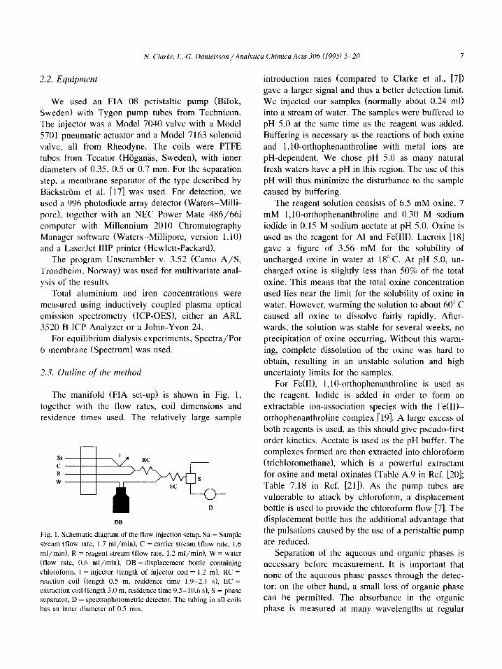
The manifold (FIA set-up) is shown in Fig. 1,

together with the flow rates, coil dimensions and

residence times used. The relatively large sample

DB

Fig. 1. Schematic diagram of the flow injection setup. Sa = Sample

stream (flow rate, 1.7 ml/min), C = carrier stream (flow rate, 1.6

ml/min), R = reagent stream (flow rate, 1.2 ml/min), W = water

(flow rate, 0.6 ml/min), DB = displacement bottle containing

chloroform, I = injector (length of injector coil = 1.2 m), RC =

reaction coil (length 0.5 m, residcncc time 1.9-2.1 s), EC =

extraction coil (length 3.0 m, residence time 9.5-10.6 s), S = phase

separator, D = spectrophotometric detector. The tubing in all coils

has an inner diameter of 0.5 mm.

introduction rates (compared to Clarke et al., [7])

gave a larger signal and thus a better detection limit. We injected our samples (normally about 0.24 ml>

into a stream of water. The samples were buffered to pH 5.0 at the same time as the reagent was added.

Buffering is necessary as the reactions of both oxine

and l,lO-orthophenanthroline with metal ions are

pH-dependent. We chose pH 5.0 as many natural

fresh waters have a pH in this region. The use of this

pH will thus minimize the disturbance to the sample

caused by buffering. The reagent solution consists of 6.5 mM oxine, 7

mM l,lO-orthophenanthroline and 0.30 M sodium

iodide in 0.15 M sodium acetate at pH 5.0. Oxine is used as the reagent for Al and Fe(III). Lacroix [18] gave a figure of 3.56 mM for the solubility of

uncharged oxine in water at 18” C. At pH 5.0, uncharged oxine is slightly less than 50% of the total

oxine. This means that the total oxine concentration

used lies near the limit for the solubility of oxine in

water. However, warming the solution to about 60” C caused all oxine to dissolve fairly rapidly. After-

wards, the solution was stable for several weeks, no

precipitation of oxine occurring. Without this warming, complete dissolution of the oxine was hard to

obtain, resulting in an unstable solution and high uncertainty limits for the samples.

For Fe(II), l,lO-orthophenanthroline is used as the reagent. Iodide is added in order to form an

extractable ion-association species with the Fe(II)-

orthophenanthroline complex [19]. A large excess of

both reagents is used. as this should give pseudo-first

order kinetics. Acetate is used as the pH buffer. The

complexes formed are then extracted into chloroform (trichloromethane), which is a powerful extractant

for oxine and metal oxinates (Table A.9 in Ref. [20];

Table 7.18 in Ref. [21]). As the pump tubes are vulnerable to attack by chloroform, a displacement bottle is used to provide the chloroform flow [7]. The displacement bottle has the additional advantage that the pulsations caused by the use of a peristaltic pump are reduced.

Separation of the aqueous and organic phases is necessary before measurement. It is important that none of the aqueous phase passes through the detector; on the other hand, a small loss of organic phase can be permitted. The absorbance in the organic phase is measured at many wavelengths at regular

8 N. Clarke, L.-G. Danirlsson/Analytica Chimica Acta 306 (1995) 5-20

intervals from 350 to 650 nm, at a rate of five

complete spectra/s. 12 or 13 wavelengths at regular intervals from 376 or 353 nm respectively, up to 630

nm are used for evaluation of the results. The noise

level at 353 nm tended to be rather high, due pre-

sumably to absorption by oxine. This meant that a

better result could often be achieved by ignoring this

first wavelength. It might be possible to use fewer than 12 wavelengths, although this would probably

decrease the predictive power of the model.

The signals (absorbances) at each wavelength are integrated, so that the peak areas are obtained. As

each sample is injected four times, the mean peak area for each sample at each wavelength is then

calculated, the contributions to the signal from Al,

Fe(U) and Fe(II1) then being separated using multivariate analysis. The multivariate method used is

partial least squares (PLS). In this method, a model

is obtained giving the best correlations between two matrices, one (the X matrix) containing the mean

peak areas after blank correction at different wave-

lengths for the standard solutions, the other (the Y matrix) containing the concentrations of the three

components in these solutions. The model obtained is then used to calculate (or predict) the concentra-

tions present in unknown samples, based on the

mean peak areas obtained at the different wave-

lengths (the prediction matrix). Although the matri-

ces are mean centred, they are not scaled, as this is unnecessary when all variables in a block are mea-

sured in the same units [22].

3. Results and discussion

In the method of Clarke et al. [6,7], iron is masked using hydroxylamine and 1, IO-orthophenanthroline, thus preventing its reaction with ox-

ine. By leaving out the masking reagent and measur-

ing at more than one wavelength, it should be possible to measure both aluminium and iron [4,23]. However, using oxine alone, it is not possible to measure both iron(I1) and iron(II1). At a pH below 4, no extraction is observed in the case of iron(H), while at higher pH values, iron(I1) is oxidized to iron(II1) (p. 587 in Ref. [21]).

Attempts to use a single-phase system, with 8-hydroxyquinoline-5-sulphonic acid as reagent for Al,

Fe(II1) and Fe(II), showed that it was possible to separate signals from the three components. How-

ever, the method proved to be impractical for use

with natural waters. The method is described in more detail by Clarke [l].

Acetate was used as the pH buffer. No problems due to the formation of acetato complexes with iron

or aluminium were observed. This is because the

reagents form much stronger complexes with the metals than acetate does.

The oxinates of Al and Fe(II1) are fairly insoluble in water, so it is necessary to extract them into an

organic solvent before measurement. Chloroform was used as the solvent. We found that an extraction time

of about 10 s gave good results. Extraction has the added advantage of enabling the sample to become

more concentrated by extracting from a relatively

large volume of water to a smaller volume of organic solvent, thus improving the detection limit. Also,

extraction minimizes interference due to absorption by humic substances. Humic substances may, how-

ever, irlterfere in another way, as their behaviour as

surfactants may influence the segmentation [24]. This will result in a larger standard deviation for samples containing large quantities of them.

In order to be able to determine both iron(U) and

iron(III), a second reagent was necessary. l,lO-Or- thophenanthroline is an often used reagent for the

determination of iron( the complex formed be-

tween the two being non-extractable. However, the iron(l,lO-orthophenanthroline complex forms

extractable ion-association species with some anions [25]. Among these is iodide [19]. A large excess of

iodide is necessary to obtain a high degree of extraction; however, no improvement was found for iodide concentrations above 0.3 M.

Iodide forms fairly strong complexes with Fe”’ [26]. However, we believe that it is unlikely that these complexes will be formed in significant

amounts in the present system, as oxine forms much

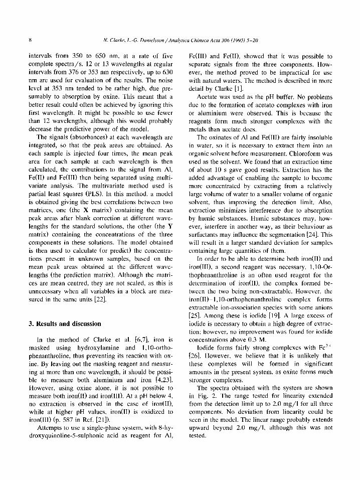
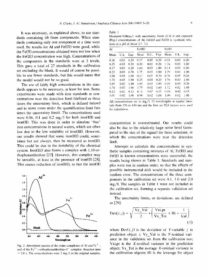
stronger complexes. The spectra obtained with the system are shown

in Fig. 2. The range tested for linearity extended from the detection limit up to 2.0 mg/l for all three components. No deviation from linearity could be seen in the model. The linear range probably extends upward beyond 2.0 mg/l, although this was not tested.

N. Clarke, L.-G. Danielsson/Anal~tica Ckimicu Acta 306 (199.5) S-20 9

It was necessary, as explained above, to use standards containing all three components. When standards containing only one component at a time were

used, the results for Al and Fe(III) were good, while

the Fe(I1) concentrations obtained were too low when the Fe(Il1) concentration was high. Concentrations of

the components in the standards were at 3 levels.

This gave a total of 27 standards in the calibration

set excluding the blank. It would of course be possi-

ble to use fewer standards, but this would mean that

the model would not be so good. The use of fairly high concentrations in the stan-

dards appears to be necessary, at least for iron. Some experiments were made with iron standards at con-

centrations near the detection limit (defined as three

times the uncertainty limit, which is defined below) and in some cases under the quantification limit (ten

times the uncertainty limit). The concentrations used

were 0.06, 0.1 and 0.2 mg/l for both iron(II1) and iron(I1). This was done in order to simulate ‘free’

iron concentrations in natural waters, which are often

low due to the low solubility of iron(II1). However,

our results showed that some iron(II1) could, some- times but not always, then be measured as iron(I1). This could be due to the instability of the chemical system. Iron(II1) also forms a complex with l,lO-or-

thophenanthroline [27]. However, this complex may

be unstable, at least in the presence of iron(I1) [28]. This causes reduction of iron(III), so that the iron(I1)

1.6

0.6 -

0.4 - Fe3+

0.2 -

Fig. 2. Absorption spectra of the wine complexes of Al and Fe3+,

and of the Fc’+ -orthophenanthroline-I- complex. Reaction time

= 2.0 s. The concentrations were 2 mg/l in the original samples.

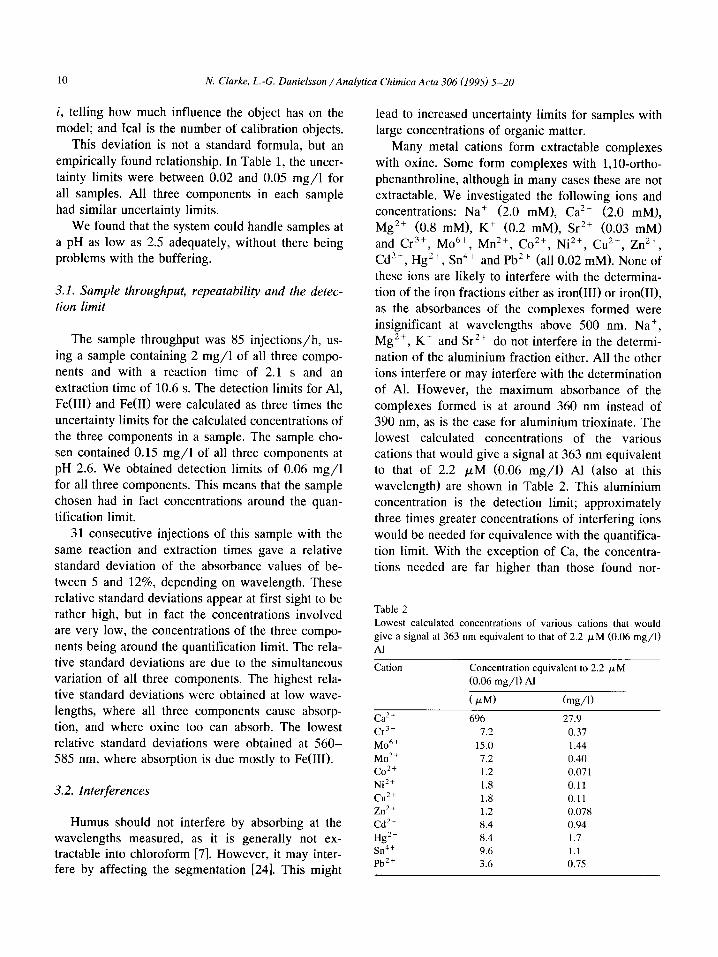
Table 1 Measured ((Meas.), with uncertainty limits (U.L.)) and expected

(Exp.) concentrations of Al, Fc(II1) and Fe(lI) in synthetic solu-

tions at a pH of about 2.5-2.6

Al Fe(III) Fc(II)

Meas. U.L. Exp. Mcas. U.L. Exp. Meas. U.L. Exp.

0.18 0.03 0.20 0.17 0.03 0.20 0.24 0.03 0.20

0.25 0.03 0.20 0.20 0.03 0.20 I .74 0.03 1.80

0.17 0.03 0.20 I.XO 0.03 1.80 0.11 0.03 0.20

0.23 0.03 0.20 1.75 0.03 I .80 1.7’) 0.03 I .80

1 .x0 0.05 I.XO 0.17 0.05 0.20 0.2h 0.05 0.20

1.7x 0.03 I .x0 0.25 0.03 0.20 1.78 0.03 I .x0

I Xi 0.03 I .x0 I .x5 0.03 I .x0 0.18 0.03 0.20

I .74 0.02 I .x0 1.75 0.02 I .x0 I .72 0.02 I .x0 0.13 0.02 0.15 0. I I 0.03 0.15 0.1s 0.02 0. I5

1.01 0.02 I .OO 0.0X 0.02 I .oo I .oo 0.02 I .oo

All concentrations arc in mg/l. 12 wavclcngths at regular inter-

vals from 376 to 630 nm and the first six PLS tactors wcrc used

for calculation.

concentration is overestimated. Our results could

also be due to the relatively large noise level (compared to the size of the signal) for these solutions, in

which the concentrations were near the detection

limit. Attempts to calculate the concentrations in syn-

thetic samples containing mixtures of Al, Fe(III) and

Fe(U) in known concentrations were successful, the results being shown in Table 1. Standards and sam-

ples were run in random order, so that the effects of

possible instrumental drift would be included in the

random error. The concentrations of the three com-

ponents in the calibration set were 0.1, 1.0 and 2.0

mg/l. The samples in Table 1 were not included in the calibration set, forming a separate validation set

instead. The uncertainty limits, or deviations, are defined

as [29]:

Vy_Val Vxi,pr -*-

2 i -

I

Vx Tot +Hi+G

1

(1)

where Dev(i, j) is the deviation of Y-variable j in

prediction object i; Vy_Val is the Y-residual variance in the validation set from the calibration run; Vxi,pr is the X-residual variance in the prediction object; Vx Tot is the average X-residual variance in the calibration objects; Hi is the leverage for object

10 N. Clarke, L.-G. Danielsson /Analytica Chimica Acta 306 (1995) 5-20

i, telling how much influence the object has on the lead to increased uncertainty limits for samples with model; and Ical is the number of calibration objects. large concentrations of organic matter.

This deviation is not a standard formula, but an

empirically found relationship. In Table 1, the uncer-

tainty limits were between 0.02 and 0.05 mg/l for

all samples. All three components in each sample had similar uncertainty limits.

We found that the system could handle samples at a pH as low as 2.5 adequately, without there being

problems with the buffering.

3.1. Sample throughput, repeatability and the detec-

tion limit

The sample throughput was 85 injections/h, using a sample containing 2 mg/l of all three compo-

nents and with a reaction time of 2.1 s and an

extraction time of 10.6 s. The detection limits for Al,

Fe(II1) and Fe(I1) were calculated as three times the uncertainty limits for the calculated concentrations of

the three components in a sample. The sample chosen contained 0.15 mg/l of all three components at pH 2.6. We obtained detection limits of 0.06 mg/l

for all three components. This means that the sample

chosen had in fact concentrations around the quantification limit.

31 consecutive injections of this sample with the same reaction and extraction times gave a relative

standard deviation of the absorbance values of be-

tween 5 and 12%, depending on wavelength. These relative standard deviations appear at first sight to be

rather high, but in fact the concentrations involved are very low, the concentrations of the three compo-

nents being around the quantification limit. The relative standard deviations are due to the simultaneous variation of all three components. The highest relative standard deviations were obtained at low wave-

lengths, where all three components cause absorption, and where oxine too can absorb. The lowest

relative standard deviations were obtained at 560- 585 nm, where absorption is due mostly to Fe(III).

Many metal cations form extractable complexes

with oxine. Some form complexes with l,lO-ortho-

phenanthroline, although in many cases these are not extractable. We investigated the following ions and

concentrations: Na+ (2.0 mM), Ca*+ (2.0 mM),

Mg*+ (0.8 mM), K+ (0.2 mM), Sr*+ (0.03 mM) and Cr3+, MO”, Mn”, Co*+, Ni2+, CU*+, Zn*+,

Cd”+, Hg2’, Sn4+ and Pb2+ (all 0.02 mM). None of

these ions are likely to interfere with the determination of the iron fractions either as iron(III) or iron(

as the absorbances of the complexes formed were insignificant at wavelengths above 500 nm. Na+,

Mg”+, K+ and Sr*+ do not interfere in the determi-

nation of the aluminium fraction either. All the other

ions interfere or may interfere with the determination

of Al. However, the maximum absorbance of the complexes formed is at around 360 nm instead of 390 nm, as is the case for aluminium trioxinate. The

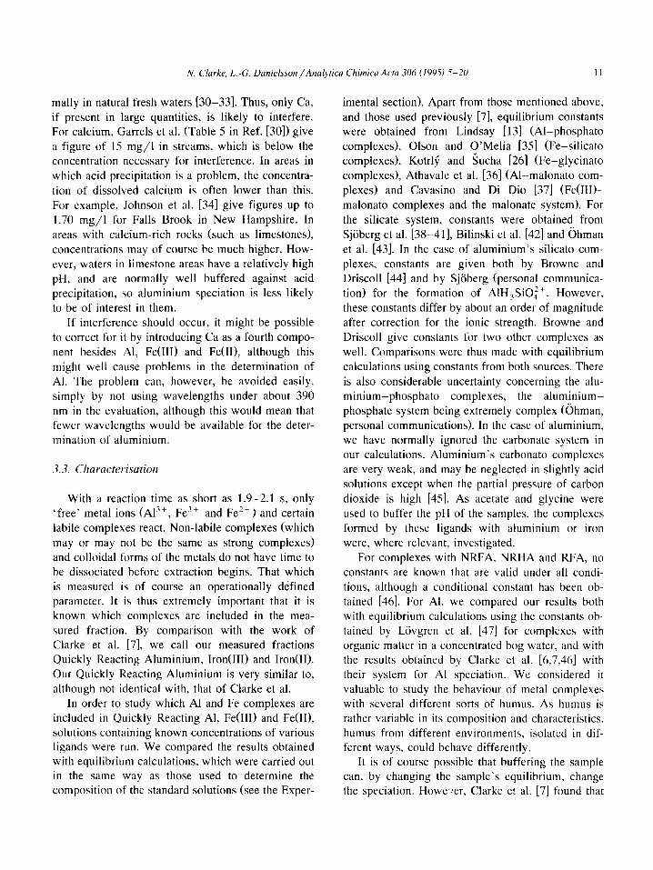
lowest calculated concentrations of the various cations that would give a signal at 363 nm equivalent

to that of 2.2 PM (0.06 mg/l) Al (also at this wavelength) are shown in Table 2. This aluminium

concentration is the detection limit; approximately three times greater concentrations of interfering ions

would be needed for equivalence with the quantifica-

tion limit. With the exception of Ca, the concentra-

tions needed are far higher than those found nor-

Table 2

Lowest calculated concentrations of various cations that would

give a signal at 363 nm equivalent to that of 2.2 pM (0.06 mg/l)

Al

Cation Concentration equivalent to 2.2 pM

(0.06 mg/l) Al

3.2. Interferences

Humus should not interfere by absorbing at the wavelengths measured, as it is generally not extractable into chloroform [7]. However, it may interfere by affecting the segmentation [24]. This might

Ca*+

cr’+

Mob+

Mn”

co*+ Ni?’

cu*+

ZI?+

Cd’+

Hg*+

Sn4+ Pb2+

( /.LM) (mg/l)

696 27.9

7.2 0.37

15.0 1.44

7.2 0.40

1.2 0.071

1.8 0.11

1.8 0.11

1.2 0.078

8.4 0.94

8.4 1.7

9.6 1.1

3.6 0.75

N. Clarke, L-G. Danielsson/Analytica Chimica Acta 306 (199-i) S-20 II

mally in natural fresh waters [30-331. Thus, only Ca, if present in large quantities, is likely to interfere. For calcium, Garrels et al. (Table 5 in Ref. [30]) give

a figure of 15 mg/l in streams, which is below the concentration necessary for interference. In areas in

which acid precipitation is a problem, the concentration of dissolved calcium is often lower than this.

For example, Johnson et al. [34] give figures up to

1.70 mg/l for Falls Brook in New Hampshire. In

areas with calcium-rich rocks (such as limestones),

concentrations may of course be much higher. How- ever, waters in limestone areas have a relatively high pH, and are normally well buffered against acid precipitation, so aluminium speciation is less likely

to be of interest in them. If interference should occur, it might be possible

to correct for it by introducing Ca as a fourth compo-

nent besides Al, Fe(III1 and Fe(B), although this might well cause problems in the determination of

Al. The problem can, however, be avoided easily, simply by not using wavelengths under about 390

nm in the evaluation, although this would mean that fewer wavelengths would be available for the determination of aluminium.

3.3. Characterisation

With a reaction time as short as 1.9-2.1 s, only ‘free’ metal ions (Al’+, Fe”+ and Fe” 1 and certain

labile complexes react. Non-labile complexes (which

may or may not be the same as strong complexes) and colloidal forms of the metals do not have time to be dissociated before extraction begins. That which

is measured is of course an operationally defined parameter. It is thus extremely important that it is known which complexes are included in the mea-

sured fraction. By comparison with the work of Clarke et al. [7], we call our measured fractions Quickly Reacting Aluminium, Iron(III) and Iron(B).

Our Quickly Reacting Aluminium is very similar to, although not identical with, that of Clarke et al.

In order to study which Al and Fe complexes are

included in Quickly Reacting Al, Fe(III) and Fe(B), solutions containing known concentrations of various ligands were run. We compared the results obtained with equilibrium calculations, which were carried out in the same way as those used to determine the composition of the standard solutions (see the Exper-

imental section). Apart from those mentioned above, and those used previously [7], equilibrium constants were obtained from Lindsay [13] (Al-phosphato

complexes), Olson and O’Melia [35] (Fe-silicato complexes), Kotrly and Sucha [26] (Fe-glycinato

complexes), Athavale et al. [36] (Al-malonato com-

plexes) and Cavasino and Di Dio [37] (Fe(IIIl-

malonato complexes and the malonate system). For

the silicate system, constants were obtained from

Sjiiberg et al. [38-411, Bilinski et al. [42] and ehman et al. [43]. In the case of aluminium’s silicato com-

plexes, constants are given both by Browne and Driscoll [44] and by Sjiiberg (personal communica-

tion) for the formation of AlH,SiO,“+. However. these constants differ by about an order of magnitude

after correction for the ionic strength. Browne and

Driscoll give constants for two other complexes as

well. Comparisons were thus made with equilibrium calculations using constants from both sources. There

is also considerable uncertainty concerning the aluminium-phosphato complexes, the aluminium-

phosphate system being extremely complex (Ghman,

personal communications). In the case of aluminium, we have normally ignored the carbonate system in our calculations. Aluminium’s carbonato complexes

are very weak, and may be neglected in slightly acid

solutions except when the partial pressure of carbon dioxide is high [45]. As acetate and glycine were

used to buffer the pH of the samples, the complexes

formed by these ligands with aluminium or iron

were, where relevant, investigated. For complexes with NRFA, NRHA and RFA, no

constants are known that are valid under all conditions, although a conditional constant has been ob-

tained [46]. For Al, we compared our results both with equilibrium calculations using the constants ob-

tained by Lovgren et al. [47] for complexes with organic matter in a concentrated bog water, and with the results obtained by Clarke et al. [6,7,46] with their system for Al speciation. We considered it

valuable to study the behaviour of metal complexes with several different sorts of humus. As humus is rather variable in its composition and characteristics,

humus from different environments, isolated in different ways, could behave differently.

It is of course possible that buffering the sample can, by changing the sample’s equilibrium, change the speciation. Howe./er, Clarke et al. [7] found that


this was not a problem for samples at a pH > 3.5, even in the presence of such a strong ligand as

citrate. Our system is likely to be less troubled by

such problems, as the sample is buffered at the same

time as the reagent is added, rather than before, as

was the case with the system of Clarke et al. [7].

For the characterisation experiments, we consid-

ered it unnecessary to use as many wavelengths as for normal runs, as the number of components to be determined was lower. For solutions containing aluminium only, a single wavelength at 388 nm was

sufficient. In the case of iron, which could occur

either as iron(III) or iron( 11 wavelengths were

used, at regular intervals from 391 to 627 nm.

Fairly low concentrations were used, in order that

the concentrations of Quickly Reacting metals might be near to those actually found in natural waters.

This is important, as the complexes present can depend on the concentrations. A drawback with the

use of low concentrations was that the spread in the results could be quite large.

The aluminium characterisation experiments were carried out using samples at a pH between 3.3 and

5.5, with the exception of some samples at pH

7.9-10.0 used to study the reaction of AI(O The

pH was buffered using acetate/acetic acid at a concentration of either 3 mM (for solutions containing

humic substances) or 10 mM for other solutions. No

pH buffer was used for the samples at pH 7.9-10.0. Except in the case of samples containing humic

substances, an ionic strength of 0.1 M, obtained using NaNO,, was used. At this ionic strength, the small variations in ionic strength caused by different

concentrations of the cations and of the ligands should be relatively insignificant, making compari-

son with equilibrium calculations straightforward. The ionic strength of solutions containing humic

substances was not adjusted, so that it should be as near as possible to that of natural fresh waters. Of

course, the presence of the 3 mM pH buffer meant that the ionic strength of these solutions was still higher than that of most natural fresh waters. For the study of aluminium’s carbonato complexes, a high partial pressure of carbon dioxide was needed, which we obtained by passing carbon dioxide gas through the samples. This should give a partial pressure of carbon dioxide equal to 1 atm. The aluminium concentration used was 37.1 PM (1.0 mg/l). All solu-

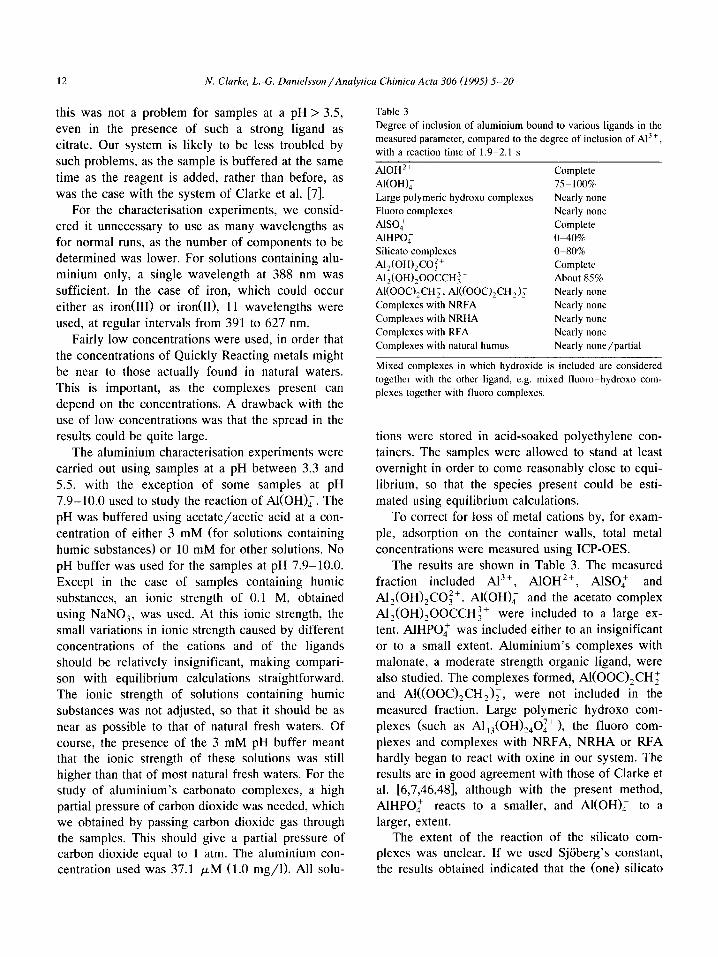
Table 3

Degree of inclusion of aluminium bound to various ligands in the

measured parameter, compared to the degree of inclusion of A13+,

with a reaction time of 1.9-2.1 s

AlOH’+

AI(

Large polymeric hydroxo complexes

Fluoro complexes

Also:

AIHPO:

Silicato complexes

A12(OH)2CO:+

A12(OH)200CCH:+

Al(OOC),CH;, AI((OOC)$H,); Complexes with NRFA

Complexes with NRHA

Complexes with RFA

Complexes with natural humus

Complete

75-100%

Nearly none

Nearly none

Complete

O-40%

O-80%

Complete

About 85%

Nearly none

Nearly none

Nearly none

Nearly none

Nearly none/partial

Mixed complexes in which hydroxide is included arc considered

together with the other ligand, e.g. mixed fluoro-hydroxo com-

plexes together with fluoro complexes,

tions were stored in acid-soaked polyethylene con-

tainers. The samples were allowed to stand at least overnight in order to come reasonably close to equi-

librium, so that the species present could be esti- mated using equilibrium calculations.

To correct for loss of metal cations by, for exam-

ple, adsorption on the container walls, total metal concentrations were measured using ICP-OES.

The results are shown in Table 3. The measured

fraction included A13+, AlOH*+, AlSO: and

Al,(OH),CO, . 2-t Al(OH), and the acetato complex

A12(OH)200CCH;+ were included to a large extent. AlHPOl was included either to an insignificant

or to a small extent. Aluminium’s complexes with malonate, a moderate strength organic ligand, were also studied. The complexes formed, A1(00C)2CHl

and A1((OOC),CHZ);, were not included in the measured fraction. Large polymeric hydroxo com-

plexes (such as Al,,(OH),,O~+), the fluoro complexes and complexes with NRFA, NRHA or RFA hardly began to react with oxine in our system. The results are in good agreement with those of Clarke et al. [6,7,46,48], although with the present method, AlHPOl reacts to a smaller, and Al(OH), to a larger, extent.

The extent of the reaction of the silicato complexes was unclear. If we used Sjoberg’s constant, the results obtained indicated that the (one) silicato

N. Clarke. L-G. Daniel.won /Analytica Chimica Acta 306 (I 993) S-20 I.3

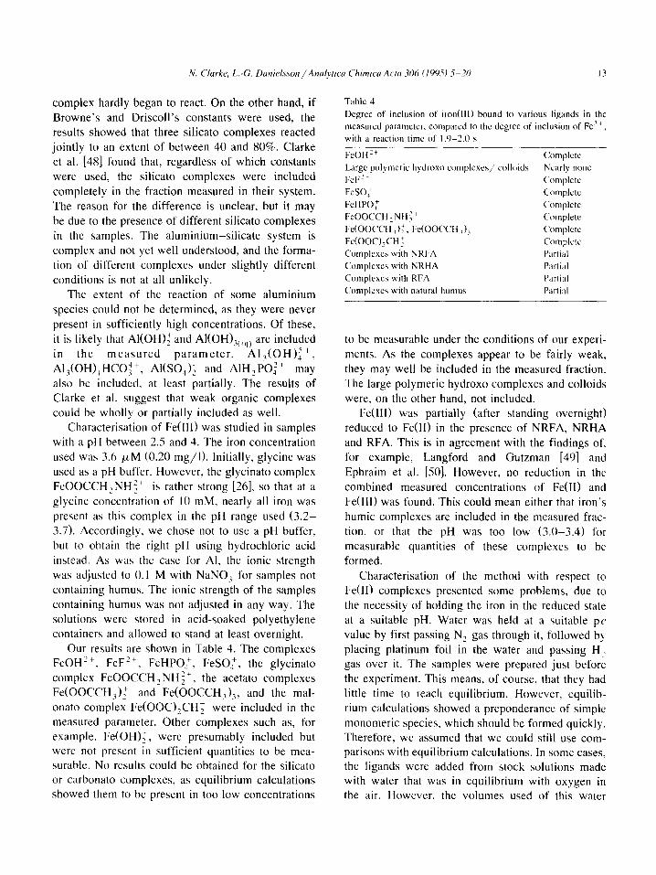
complex hardly began to react. On the other hand, if Browne’s and Driscoll’s constants were used, the results showed that three silicato complexes reacted

jointly to an extent of between 40 and 80%. Clarke

et al. [48] found that, regardless of which constants were used, the silicato complexes were included

completely in the fraction measured in their system.

The reason for the difference is unclear, but it may be due to the presence of different silicato complexes

in the samples. The aluminium-silicate system is complex and not yet well understood, and the forma-

tion of different complexes under slightly different conditions is not at all unlikely.

The extent of the reaction of some aluminium species could not be determined, as they were never

present in sufficiently high concentrations. Of these,

it is likely that AI( and AI(OH), are included

in the measured parameter. Al,(OH)z ‘,

Al &OH), HCO: + , Al(SO,); and AlH,POi’ may

also be included. at least partially. The results of Clarke et al. suggest that weak organic complexes

could be wholly or partially included as well. Characterisation of Fe(II1) was studied in samples

with a pH between 2.5 and 4. The iron concentration

used was 3.6 PM (0.20 mg/l). Initially, glycine was

used as a pH buffer. However, the glycinato complex FeOOCCH,NH:’ is rather strong [26], so that at a

glycine concentration of 10 mM, nearly all iron was

present as this complex in the pH range used (3.2- 3.7). Accordingly, we chose not to use a pH buffer,

but to obtain the right pH using hydrochloric acid instead. As was the case for Al, the ionic strength

was adjusted to 0.1 M with NaNO, for samples not containing humus. The ionic strength of the samples

containing humus was not adjusted in any way. The solutions were stored in acid-soaked polyethylene containers and allowed to stand at least overnight.

Our results are shown in Table 4. The complexes FeOH’+, FeF”, FeHPO,f, FeSO:, the glycinato

complex FeOOCCH2 NH z + , the acetato complexes Fe(OOCCH,)f and Fe(OOCCH,),, and the mal-

onato complex Fe(OOC),CH; were included in the measured parameter. Other complexes such as, for example, Fe(OH)i , were presumably included but were not present in sufficient quantities to be measurable. No results could be obtained for the silicato or carbonato complexes, as equilibrium calculations showed them to be present in too low concentrations

Table 4

Degree of inclusion of iron bound to various ligands in the

measured paramctcr. compared to the degree of inclusion of Fe”+,


FeOH’+ Complete

Large polymeric hydroxo complexes/ colloids Nearly none

FcF” Complete

FcSO; Complctc

FeHPO: Complete

FcOOCCH NH’ + 7

Fc(OOCC;, ,?’ .-Fc(OOCCH ?jl

(‘omplete

Cornpick

Fe(OOC),CH;

Complcxca with NRFA

Complcxcs with NRHA

Complexes with RFA

Complexes with natural humus

Complete

Partial

Partial

Partial

Partial

to be measurable under the conditions of our experi-

ments. As the complexes appear to be fairly weak, they may well be included in the measured fraction.

The large polymeric hydroxo complexes and colloids were, on the other hand, not included.

Fe(III) was partially (after standing overnight) reduced to Fe(II) in the presence of NRFA, NRHA

and RFA. This is in agreement with the findings of. for example, Langford and Gutzman [49] and

Ephraim et al. [%)I. However, no reduction in the

combined measured concentrations of Fe(II) and Fe(III) was found. This could mean either that iron’s

humic complexes are included in the measured frac-

tion, or that the pH was too low (3.0-3.4) for measurable quantities of these complexes to be

formed.

Characterisation of the method with respect to Fe(II) complexes presented some problems, due to the necessity of holding the iron in the reduced state

at a suitable pH. Water was held at a suitable p’ value by first passing N, gas through it, followed by

placing platinum foil in the water and passing H1 gas over it. The samples were prepared just before

the experiment. This means, of course, that they had little time to reach equilibrium. However, equilib-

rium calculations showed a preponderance of simple monomeric species, which should be formed quickly.

Therefore, we assumed that we could still use comparisons with equilibrium calculations. In some cases, the ligands were added from stock solutions made with water that was in equilibrium with oxygen in the air. However. the volumes used of this water

14 N. Clarke, L.-G. Danielson /Analytica Chimica Acta 306 (1995) 5-20

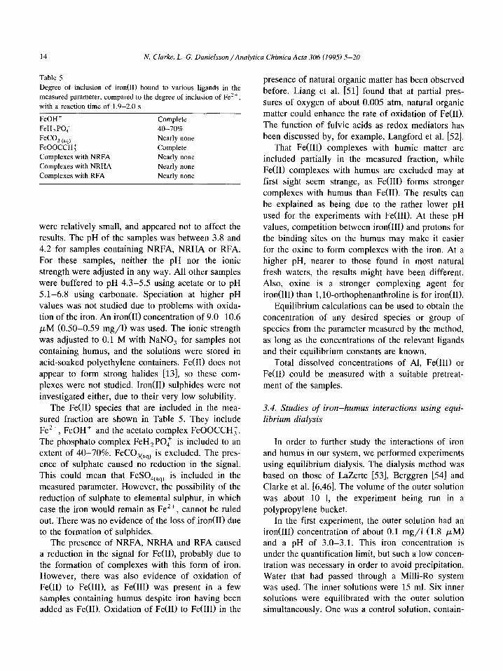
Table 5

Degree of inclusion of iron bound to various ligands in the

measured parameter, compared to the degree of inclusion of Fe*‘,


FeOH+

FeH,PO:

FeCO, (aqj FeOOCCHl

Complexes with NRFA

Complexes with NRHA

Complexes with RFA

Complete

40-70%

Nearly none

Complete

Nearly none

Nearly none

Nearly none

were relatively small, and appeared not to affect the

results. The pH of the samples was between 3.8 and 4.2 for samples containing NRFA, NRHA or RFA.

For these samples, neither the pH nor the ionic strength were adjusted in any way. All other samples were buffered to pH 4.3-5.5 using acetate or to pH

5.1-6.8 using carbonate. Speciation at higher pH values was not studied due to problems with oxida-

tion of the iron. An iron(B) concentration of 9.0-10.6

PM (0.50-0.59 mg/l) was used. The ionic strength

was adjusted to 0.1 M with NaNO, for samples not

containing humus, and the solutions were stored in

acid-soaked polyethylene containers. Fe(I1) does not appear to form strong halides [13], so these com-

plexes were not studied. Iron(I1) sulphides were not investigated either, due to their very low solubility.

The Fe(I1) species that are included in the measured fraction are shown in Table 5. They include

Fe’+, FeOH+ and the acetato complex FeOOCCH_T. The phosphato complex FeH,PO,f is included to an

extent of 40-70%. FeCO,(,,, is excluded. The presence of sulphate caused no reduction in the signal. This could mean that FeSO,r,,, is included in the

measured parameter. However, the possibility of the reduction of sulphate to elemental sulphur, in which case the iron would remain as Fe”+, cannot be ruled

out. There was no evidence of the loss of iron(I1) due to the formation of sulphides.

The presence of NRFA, NRHA and RFA caused a reduction in the signal for Fe(II), probably due to the formation of complexes with this form of iron. However, there was also evidence of oxidation of

Fe(I1) to Fe(III), as Fe(II1) was present in a few samples containing humus despite iron having been added as Fe(I1). Oxidation of Fe(I1) to Fe(II1) in the

presence of natural organic matter has been observed

before. Liang et al. 1511 found that at partial pres-

sures of oxygen of about 0.005 atm, natural organic matter could enhance the rate of oxidation of Fe(I1).

The function of fulvic acids as redox mediators has

been discussed by, for example, Langford et al. [52]. That Fe(II1) complexes with humic matter are

included partially in the measured fraction, while

Fe(I1) complexes with humus are excluded may at first sight seem strange, as Fe(II1) forms stronger

complexes with humus than Fe(I1). The results can

be explained as being due to the rather lower pH

used for the experiments with Fe(II1). At these pH

values, competition between iron(II1) and protons for the binding sites on the humus may make it easier

for the oxine to form complexes with the iron. At a higher pH, nearer to those found in most natural fresh waters, the results might have been different. Also, oxine is a stronger complexing agent for

iron(II1) than 1, lo-orthophenanthroline is for iron(I1). Equilibrium calculations can be used to obtain the

concentration of any desired species or group of

species from the parameter measured by the method,

as long as the concentrations of the relevant ligands and their equilibrium constants are known.

Total dissolved concentrations of Al, Fe(II1) or Fe(I1) could be measured with a suitable pretreat-

ment of the samples.

3.4. Studies of iron-humus interactions using equi-

librium dialysis

In order to further study the interactions of iron and humus in our system, we performed experiments using equilibrium dialysis. The dialysis method was

based on those of LaZerte [53], Berggren 1541 and Clarke et al. [6,46]. The volume of the outer solution

was about 10 1, the experiment being run in a polypropylene bucket.

In the first experiment, the outer solution had an iron(II1) concentration of about 0.1 mg/l (1.8 ,uM) and a pH of 3.0-3.1. This iron concentration is under the quantification limit, but such a low concentration was necessary in order to avoid precipitation. Water that had passed through a Milli-Ro system was used. The inner solutions were 15 ml. Six inner solutions were equilibrated with the outer solution simultaneously. One was a control solution, contain-

N. Clarke, L.-G. Danielsson / Analytica Chimica Acta 306 (199.5) 5-20 15

ing only water that had passed through a Modulab system. Others contained 23 mg/l of NRFA, 16

mg/l of NRHA or 21 mg/l of RFA. In addition,

two samples of natural humus-rich water were used. These samples, called GII and Damm A, were from

surface waters in Masbybacken and Svartbticken,

both in Sweden, respectively. The inner solutions were acidified to about the same pH as the outer solution, in order to prevent the precipitation of iron

on the membrane. A cellulose ester membrane, Spec- tra/Por 6, with a nominal molecular weight cut-off

of 1000 was used. The equilibration time was about

142 h. During equilibration, the solutions were

shaken at 60 rpm using a Lab Shaker (Kihner, Basel). The temperature during the experiment was

20.2-20.4” C. After the experiment, the concentrations in the inner and outer solutions were measured

both with the FIA system and with ICP-OES. Ten iron standards were used, containing both iron(II1)

and iron in concentrations of 0.06, 0.1 and 0.2 mg/l, together with a blank. Standard solutions including aluminium at levels of 0.1, 0.5 and 1.0

mg/l, together with iron(II1) and iron( both at 0.1 mg/l, were also used, so as to be able to correct for the presence of aluminium if necessary. This neces-

sity did not arise. The first five PLS factors were

used for calibration.

water samples GII and Damm A (the inner solutions) were 1.94 and 0.84 mg/l, respectively after dialysis.

This iron was probably present throughout the dialy-

sis, as these samples contained total Fe concentra-

tions of 2.48 and 1.40 mg/l, respectively, after acidification but before dialysis. The concentrations measured with the FlA system were 0.42 and 0.2

mg/l Fe(II1) respectively. 0.42 mg/l was outside

the calibrated range in this experiment, but the figure is unlikely to be far wrong as it lies within the normal range for linearity. Figures for iron(I1) were

under the detection limit, although it is possible that

at least some of the iron that was excluded from the

measured fraction may have been present as iron

complexes with humus. It appears, however, that iron(II1) complexes with natural humus may be in-

cluded, at least partially, in the measured fraction. It is interesting to note that iron(II1) was not reduced in

the presence of humus in the natural water samples,

unlike in the case of the isolated humic substances.

We found that the iron concentrations in the outer solution and the control solution were about the same, measured both with the FIA system and with

ICP-OES. For the samples containing NRFA, NRHA and RFA, the total iron concentrations were 0.14, 0.15 and 0.15 mg/l, respectively. Iron concentra-

tions measured with the FIA system were 0.10, 0.08 and 0.11 mg/l, respectively, the iron being present as iron in all three cases. Although these concen-

trations lie under the quantification limit, it is probably safe to say that the concentrations determined using ICP-OES were greater than those determined

using the present method. It seems, therefore, that, at suitable concentrations and at equilibrium, these reference humic substances mediate the complete re-

duction of iron(II1) to iron(I1). The complexes formed by iron and NRFA, NRHA or RFA may be iron complexes or iron(II1) complexes or a mixture of both. In any case, they appear not to be included in the measured fraction.

In the second experiment, reducing conditions were used. The dialysis method used was much the same as that described above. The outer solution,

about 10 1, contained about 0.1 mg/l Fe. A pH of 4.2 was used, the pH being buffered using 3 mM

acetate-acetic acid. Reducing conditions were ob-

tained using the same method as in the characterisa-

tion experiments described earlier. The inner solutions were the same as in the first experiment, except

that they were not acidified. Equilibration time was about 114 h, with shaking at 50 rpm. Ten iron

standards were used, containing both iron(II1) and iron in concentrations of 0.1, 0.5 and 1.0 mg/l, together with a blank. Standard solutions including aluminium at levels of 0.1, 0.5 and 1.0 mg/l, to-

gether with iron(II1) and iron(B), both at 0.5 mg/l,

were also used, so as to be able to correct for the presence of aluminium if necessary. In this experiment, this turned out to be necessary, as sample GII

contained 0.08 mg/l (3 FM) Quickly Reacting Al after dialysis. This aluminium was presumably organic bound, so its presence means that aluminium’s humic complexes may occasionally be included in Quickly Reacting Al. Another possibility, that aluminium is released during the dissolution and reduction of Fe(OH),(,,, is less likely, as Fe(III) was not reduced in sample GII (see below).

Total iron concentrations in the natural humus-rich The first six PLS factors were used for calibra-


tion. As before, the concentrations in the outer solu-

tion and in the control solution were about the same, measured both as Quickly Reacting Fe(R) with the

FIA system and as total Fe with ICP-OES. For the samples containing NRFA, NRHA and RFA, iron

concentrations measured with ICP-OES were 0.30, 0.34 and 0.29 mg/l, respectively. Quickly Reacting

Fe(II1) concentrations were 0.07 mg/l in all three

samples, while Quickly Reacting Fe(I1) concentra-

tions were 0.10, 0.08 and 0.13 mg/l, in the NRFA, NRHA and RFA samples, respectively. The concen-

trations of Quickly Reacting Fe(R) are what would

be expected for uncomplexed Fe(U), supporting our belief that the humic complexes of Fe(R) are not

included in the measured parameter. The appearance

of Quickly Reacting Fe(II1) supports the idea that NRFA, NRHA and RFA can mediate both oxidation and reduction of iron, depending on the conditions.

The iron(III) is probably present as humic complexes, providing further evidence that these complexes are included partially in Quickly Reacting

Fe(II1). Samples GII and Damm A contained 3.45 and

1.65 mg/l total Fe respectively, after dialysis. No

Quickly Reacting Fe(R) was found. The concentrations of Quickly Reacting Fe(III) were 0.69 and 0.48 mg/l in GII and Damm A, respectively. These

results agree with those from the first dialysis experiment, the higher concentrations found here being due to the reduced competition for binding sites from

hydrogen ions. It appears certain that some Fe(II1) humic complexes can be included in Quickly React-

ing Fe(III). The results in this case do not prove the

oxidation of Fe(U), as these samples contained 2.72

and 1.44 mg/l total Fe respectively, before dialysis.

3.5. Measurements made on natural waters

Natural water samples taken from the Skjervatjern area, Norway, were analysed for Quickly Reacting

Al, Fe(II1) and Fe(R) using the FIA system, and for

total Al and Fe using ICP-OES (determined by Ann-Catrine Norrstriim, of the Division of Land and

Water Resources, the Royal Institute of Technology).

These samples were taken from different environments, including lake, peat and ground water. The

samples and standards were run alternately in ran-

dom order. The concentrations of the three components in the standard solutions were 0.1, 0.5 and 1.0

mg/l. 28 standards, including a blank, were used. Water that had passed through a Modulab system was run as a blank for the natural water samples; the same water, acidified to the same pH as the standards, was used as a blank for these. In order to

decide how many wavelengths and PLS factors to

use in the calculations, five of the standards used

were also run as samples. It was assumed that the

model that gave the best results for these, taking both accuracy and precision into account, was the best model to use for the natural water samples as well.

12 wavelengths at regular intervals from 376 to 630 nm and the first five PLS factors were used for calculation of the Quickly Reacting concentrations.

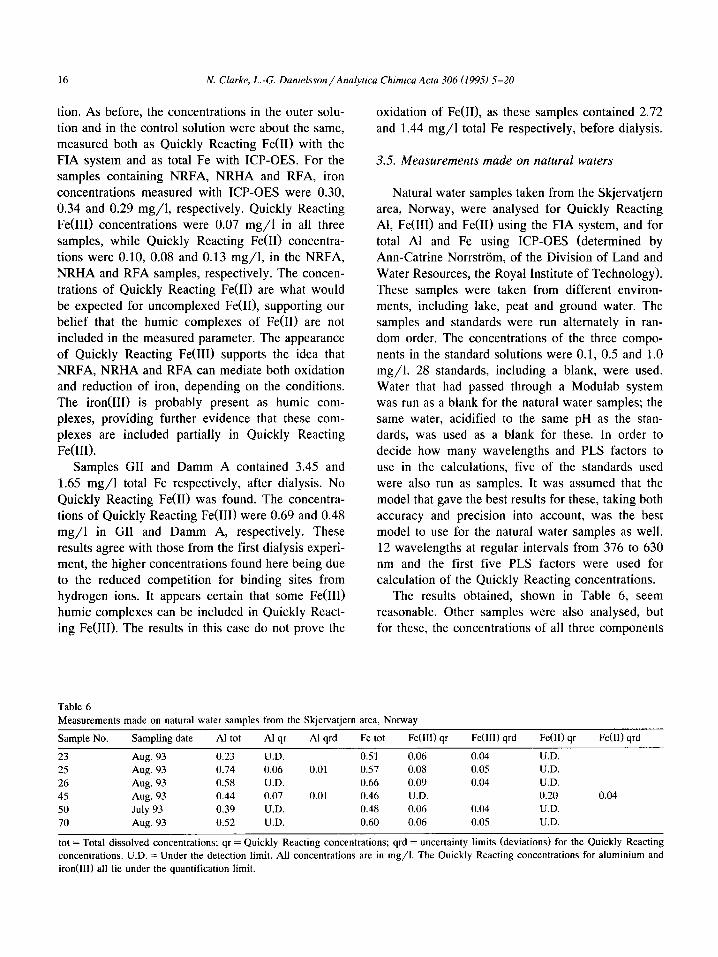
The results obtained, shown in Table 6, seem

reasonable. Other samples were also analysed, but for these, the concentrations of all three components

Table 6

Measurements made on natural water samples from the Skjervatjern area, Norway

Sample No. Sampling date Al tot Al qr Al qrd Fe tot Fe(llI) qr Fe(II1) qrd Fe(H) qr Fe(R) qrd

23 Aug. 93 0.23 U.D. 0.51 0.06 0.04 U.D.

25 Aug. 93 0.74 0.06 0.01 0.57 0.08 0.05 U.D.

26 Aug. 93 0.58 U.D. 0.66 0.09 0.04 U.D.

45 Aug. 93 0.44 0.07 0.01 0.46 U.D. 0.20 0.04

50 July 93 0.39 U.D. 0.48 0.06 0.04 U.D.

70 Aug. 93 0.52 U.D. 0.60 0.06 0.05 U.D.

tot = Total dissolved concentrations; qr = Quickly Reacting concentrations; qrd = uncertainty limits (deviations) for the Quickly Reacting

concentrations. U.D. = Under the detection limit. All concentrations are in mg/l. The Quickly Reacting concentrations for aluminium and

iron(II1) all lie under the quantification limit.

N. Clarke, L.-G. Danielsson/Analytica Chimica Acta 306 (1995) 5-20 17

were under the detection limit. The low values found

may be due to the presence of aluminium and iron in polymeric or colloidal forms.

3.6. Comparison with the method of Clarke et al. 171

A further test made on the method was a comparison of Quickly Reacting aluminium as determined using the new method with a determination using the

method of Clarke et al. [7]. Surface water samples

from Masbybacken and Svartbacken in Sweden, and from the Lysina catchment in the Czech Republic,

were used. Total dissolved aluminium and total dis-

solved silicon were determined using ICP-OES.

We used the method of Clarke et al. exactly as described, except that the reduction coil was 13 cm

long instead of 14 cm. The buffering, reaction and extraction times were slightly longer than those used by Clarke et al. (1.1, 2.8 and 5.8 s respectively,

compared with 1.0, 2.3 and 5.1 s). However, we do not believe that this should lead to significantly

different results. The experimental procedure was the same as for

the natural water samples from Skjervatjern, except that three of the standards were also used as valida-

tion samples and the first six PLS factors were used

for calculation of the Quickly Reacting concentrations of the metals.

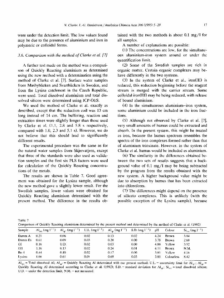
The results are shown in Table 7. Good agreement was obtained for the Lysina sample, although the new method gave a slightly lower result. For the Swedish samples, lower values were obtained for Quickly Reacting aluminium determined with the

present method. The difference in the results ob-

tamed with the two methods is about 0.1 mg/l for

all samples. A number of explanations are possible: (1) The concentrations are low, for the simultane-

ous aluminium-iron system around or under the

quantification limit. (2) Some of the Swedish samples are rich in

organic matter. Certain organic complexes may be-

have differently in the two systems. (3) In the system of Clarke et al., iron@) is

reduced, this reduction beginning before the reagent stream is merged with the carrier stream. Some

colloidal iron(III) may be being reduced, with release

of bound aluminium.

(4) In the simultaneous aluminium-iron system,

some aluminium could be included in the iron frac-

tions. (5) Although not observed by Clarke et al. [7],

very small amounts of humus could be extracted and

absorb. In the present system, this might be treated as iron, because the humus spectrum resembles the spectra of the iron complexes formed rather than that

of aluminium trioxinate. However, in the system of

Clarke et al. humus would be included as aluminium. (6) The similarity in the differences obtained be-

tween the two sets of results suggests that a back-

ground value of 0.1 mg/l may be being subtracted by the program from the results obtained with the

new system. A higher background value might be

due to absorption by humus that has been extracted into chloroform.

(7) The differences might depend on the presence of silicato complexes. This is unlikely (with the

possible exception of the Lysina sample), because

Table 7

Comparison of Quickly Reacting aluminium determined by the present method and determined by the method of Clarke et al. (1992)

Sample Al,,, (mg 1-l) Al,,, (mg 1-l) U.L. (mg I-‘) Al,, (mg I-‘) SD. (mg I-‘) pH Colour Sir,,, (mg 1-r)

Damm A 0.21 0.06 0.02 0.13 0.02 4.24 Brown 3.84

Damm Es 0.61 0.09 0.03 0.20 0.00 3.78 Brown 2.68

GI 0.16 U.D. 0.02 0.03 0.00 4.88 Yellow 3.92

GII 1.16 0.13 0.02 0.24 0.01 4.11 Brown N.M.

Bo 4 0.44 0.10 0.02 0.17 0.00 3.81 Yellow 4.16

Lysina 1.66 0.61 0.01 0.69 0.03 3.85 Colourless 8.42

Al t<,t = Total dissolved Al; Al,,, = Quickly Reacting Al determined with our present method; U.L. = uncertainty limit for Al,,,; Al,, =

Quickly Reacting Al determined according to Clarke et al. (1992); SD. = standard deviation for Al,,; Si,,,, = total dissolved silicon;

U.D. = under the detection limit, N.M. = not measured.


both the silicon and aluminium concentrations are

too low. More than one of these factors may be operating.

4. Conclusions

It is possible to measure Quickly Reacting Al,

Fe(R) and Fe(II1) simultaneously using complexation by oxine and l,lO-orthophenanthroline-iodide, fol-

lowed by extraction into chloroform, in a flow-in-

jection system. A reaction time of about 1.9-2.1 s and an extraction time of about 9.5-10.6 s gave good results. This is, as far as we know, the first

time that a method that measures these three components simultaneously has been presented. The contri-

butions to the signal from the three components can

be separated without difficulty using Partial Least Squares.

The sample throughput is 85 injections/h, and detection limits of 0.06 mg/l for all three compo-

nents were obtained. The relative standard deviation

of the absorbance for 31 consecutive injections of a standard containing 0.15 mg/l of the three compo-

nents varies from 5 to 12%, depending on wavelength. The linear range extends from the detection

limit up to at least 2 mg/l for all components. The only cation that might interfere under normal

circumstances is Ca2+. If present in concentrations of about 28 mg/l, Ca2+ gives a signal equivalent to

that of 60 pg/l Al at 363 nm, the wavelength at

which the absorbance of the calcium complex is

greatest. However, this problem can be avoided by not using wavelengths under 390 nm for evaluation.

In the case of aluminium, the most important species in the measured parameter are Al”+, A10H2+ and AlSOl. Weak organic complexes similar to the

acetato complexes could be included partially. Other weak complexes may also be included. On the other hand, large polymeric hydroxo complexes and fluoro complexes are excluded. AlHPO,f is included to an extent of O-40%. Complexes with humic or fulvic acids are almost always excluded, although excep- tions do, rarely, occur.

The Fe(III) species that are included in the measured parameter include Fe3+, FeOH’+, FeF’+, FeHPOl and FeSO:. Large polymeric hydroxo

complexes are excluded. Complexes with natural and extracted humic substances appear to be included partially.

Among the Fe(R) species that are included are Fe’+ and FeOH+. FeH,POl is included to an

extent of 40-70%. FeCO,(,,, is excluded. Com- plexes with humic and fulvic acids appear also to be excluded.

The reduction of iron(II1) to iron(U) and the

oxidation of iron(R) to iron(III), in both cases mediated by humic substances, could be demonstrated. It

appeared that the same humic substances could, under different conditions, function as promoters of either oxidation or reduction.

Results obtained with natural water samples were satisfactory.

A comparison made with the system for the determination of Quickly Reacting aluminium developed

by Clarke et al. [7] using natural water samples resulted in slightly lower values obtained with the

present system. Several explanations are possible.

The method has other potential uses as well as the measurement of Quickly Reacting Al, Fe(III) and Fe(R) in natural waters. For example, it could also

be used for the study of the interactions of Fe and Al with humic substances (including their competition for available sites), or for the study of the kinetics of

the reduction of Fe(II1) to Fe(R) and the oxidation of Fe(H) to Fe010 in the presence of humus. It should also be possible to use our method for the determina-

tion of conditional equilibrium constants for humic

complexes of iron(R) and aluminium, in the same way as Clarke et al. [46] did for the humic com-

plexes of aluminium. It might be possible to improve the system, for

example by using a smaller injection volume, as has been proposed by Berggren and Spar& [55] for the system of Clarke et al. This would make it possible to analyze samples containing much higher concentrations of aluminium and iron. Also, the effect of humic substances on the segmentation would be reduced.

It might also be possible to use fewer wavelengths in the evaluation without sacrificing accuracy. This would have the advantage of simplifying the evaluation.

By reducing the reaction time, it might be possible to obtain a different speciation.

N. Clarke, L.-G. Danielsson/Analytica Chimica Acta 306 (1995) S-20 I4

Acknowledgements

We would like to thank Bruce Kowalski, Peter Kaufmann, Steve Banwart, Olle Wahlberg and An-

ders Spar&n and other members of the Department of Analytical Chemistry at the Royal Institute of Tech-

nology for interesting and useful discussions and

suggestions, Ann-Catrine NorrstrGm for providing natural water samples and for making the ICP mea-

surements on these, Lars Lundin, Reiner Giesler and

Jakuh HruSka for providing natural water samples, Folke Ingman for helpful comments on the

manuscript, the National Swedish Environmental Protection Board for providing NRFA and NRHA,

Catharina Pettersson and Bert Allard for providing

RFA, Olle Wahlberg for the loan of platinum foil, Rolf Jansson for technical help and the National Swedish Environmental Protection Board, the Bengt Lundqvist Memorial Foundation, the OK Environ-

mental Foundation and the Futura Foundation for financial support.

References

III

[21

[31 [41

[51

[hl

[71

[Xl

[‘)I

II01

[I II

I121

[I31

N. Clarke, Ph.D. Thesis, The Royal Institute of Technology.

Stockholm, Sweden. 1994.

N. Clarke. L.-G. Danielsson and A. Spar&, Pure Appl.

Chcm.. (1995) in press.

V. Kubln, Crit. Rev. Anal. Chcm., 23 (lYY2) 15.

L.E. L&n, A. Rios, M.D. Luque de Castro and M. Val&rcel,

Lab. Robot. Autom.. I (1989) 295.

M. Blanco, J. Gene, H. Iturriaga. S. Maspoch and J. Riba,

Talanta. 34 (lY87) Y87.

N. Clarke, L.-G. Danielsson and A. Spar&, Finnish Humus

News. 3 ( I YY I ) 253.

N. Clarke, L-G. Danielsson and A. Spa&, Int. J. Environ.

Anal. (‘hem., 4X (1992) 77.

C‘. Pettcrsson, J. Ephraim and B. Allard, in C. Pettersson,

Ph.D. Thesis. University of Linkiiping, Sweden, 1992, Paper

III.

EM. l‘hurman and R.L. Malcolm, Environ. Sci. Technol., IS

( I YX I ) 463.

C. Pettcrshon. I. Arsenic, J. Ephraim, H. BorCn and B.

Allard, Sci. Total Environ.. Xl/82 (1989) 287.

N. Ingri, W. Kakolowicz. L.G. Sill& and B. Warnqvist,

Talanta, I4 (lYh7) 1261.

W. Stumm and J.J. Morgan, Aquatic Chemistry, Wilcy-lnter-

xiencc. New York, 2nd edn.. lY81.

W.L. Lindsay. Chemical Equilibria in Soils, Wiley, New

York. lY7Y.

[14] J. Bruno, W. Stumm, P. Wersin and F. Brandberg, Geochim.

Cosmochim. Acta, 56 (1992) 1139.

[IS] J. Bruno, P. Wersin and W. Stumm, Geochim. Cosmochim.

Acta, 56 (1992) 1139.

[16] G. Higg, AllmIn och oorganisk kemi. Almqvist and Wikscll.

Stockholm. 6th edn., 1963, p. 3 17.

[17] K. Bickstriim, L..-G. Danielsson and L. Nord. Anal. Chim.

Acta. 169 (1985) 43.

[IX] S. Lacroix. Anal. <‘him. Acta, I (1947) 260.

[IY] F. Vydra and R. Pribil, Talanta, 3 (IYS9) 72.

[20] A. Ringbom, Complcxation in Analytical Chemistry, Intcr-

science, New York, 1963.

[21] T. Sekine and Y. Hasegawa, Solvent Extraction Chemistry,

Fundamentals and Applications. Marcel Dekker. New York.

1977.

[22] P. Geladi and B.R. Kowalski, Anal. Chim. Acta. IX5 (19X6)

I.

[23] K. Goto, H. Tamura. M. Onodera and M. Nagatama. Talanta.

21 (IY74) 1x3.

[24] V. KubBn, L.-G. Daniclsson and F. Ingman. Anal. Chcm., 62

( 1990) 2026.

[2S] Z. Marczenko, Separation and Spcctrophotomctric Determi-

1261

[271

[281 l2Yl

[301

[311

[321

[331

[341

[3Sl

1361

I371

[3X1

[391

[401

[411

nation of Elements. Ellis Horwood. Chichester, 1986, p. 332.

S. Kotrlf and L. Sucha, Handbook of Chemical Equilibria in

Analytical Chemistry. Ellis Horwood. Chichester. 19X5. pp.

131, 156-157. 167.

A.E. Harvey Jr., J.A. Smart and ES. Amis. Anal. Chcm. 27

(IYSSI 26.

H. Fadrux and J. Ma@, Analyst, 100 (lY75) 540.

C‘amo A/S. Unscrambler II Version 35 lJscr’\ Guide, Camo

A/S, Trondheim, IYYl, p. 212.

R.M. Garrels. F.T. Mackenzie and C. Hunt, Chemical Cycles

and the Global Environment. Assessing Human Influcnccs.

William Kaufmann. Los Altos. 1975, pp. 33-35.

A.M. Shillcr and I:.A. Boyle. Geochim. Cosmochim. Acta.

51 (lYX7) 3273.

R. Rossmann and J. Barrcs. J. Great Lakes Rcs.. I4 (1988)

1X8.

K.H. Coale and AR. Flegal. Sci. Tot. Environ.. S7/NX

(1089) 2Y7.

N.M. Johnson, C.T. Driscoll, J.S. Eaton. G.E. Likens and

W.H. McDowell, Geochim. Cosmochim. Acta. 45 (lY81)

1421.

L.L. Olson and CR. O’Mclia. J. Inorg. Nucl. Chcm., 35

(lY73) 1977.

V.T. Athavalc, N. Mahadevan, P.K. Mathur and R.M. Sathc.

J. Inorg. Nucl. Chem.. 2Y (1967) 1947.

F.P. Cavasino and E. Di Dio. J. Chcm. Sot. (A). (lY7l)

3176.

S. Sjiiberg, A. Nordin and N. Ingri, Mar. C’hcm.. 10 (1YXl)

521.

S. Sjiibcrg. Y. Hagglund. A. Nordin and N. Ingri. Mar.

Chem.. I3 (1983) 35.

S. Sjiiberg, N. Ingri, A.-M. Nenncr and I..-(). ehman, Inorg.

Biochcm., 24 (1985) 267.

S. Sjiiberg, L.-O. ehman and N. Ingri, Acta Chem. Stand. A.

30 (1085) Y3.

20 N. Clarke, L.-G. Danielsson/Analytica Chimica Acta 306 (1995) 5-20

[42] H. Bilinski, L. Horvath, N. Ingri and S. Sjdberg, .I. Soil Sci., [49] C.H. Langford and D.W. Gutzman, Anal. Chim. Acta, 256

41 (1990) 119. (1992) 183.

1431 L.-O. Ghman, A. Nordin, I. Fattahpour Sedeh and S. Sjoberg,

Acta Chem. Stand., 45 (1991) 335.

[44] B.A. Browne and CT. Driscoll, Science, 256 (1992) 1667.

[45] T. Hedlund, S. Sjiiberg and L.-O. Ghman, Acta Chem.

Stand. A, 41 (1987) 197.

[50] J.H. Ephraim, A.S. Mathuthu and J.A. Marinsky, Complex

Forming Properties of Natural Organic Acids. Part 2. Com-

plexes with Iron and Calcium, Swedish Nuclear Fuel and

Waste Management Company Technical Report 90-28,

Stockholm, 1990.

[46] N. Clarke, L.-G. Danielsson and A. Spar&r, Water Air Soil

Pollut., (1995) in press.

[47] L. Lijvgren, T. Hedlund, L.-O. Ghman and S. Sjoberg, Water

Res., 21 (1987) 1401.

[51] L. Liang, J.A. McNabb, J.M. Paulk, B. Gu and J.F. Mc-

Carthy, Environ. Sci. Technol., 27 (1993) 1864.

[52] C.H. Langford, R. Ray, G.W. Quance and T.R. Khan, Anal.

Lett., 10 (1977) 1249.

[48] N. Clarke, L.-G. Danielsson, A. Hanning, F. Ingman and A.

Spar&r, in L. Maxe (Ed.), Analytical Methodology, Effects

of Acidification on Groundwater in Sweden - Hydrological

and Hydrochemical Processes, Final Report II of the Inte-

grated Groundwater Acidification Project, 1994, pp. 9-14.

[53] B.D. LaZerte, Can. J. Fish. Aquat. Sci., 41 (1984) 766.

[54] D. Berggren, Int. J. Environ. Anal. Chem., 35 (1989) 1.

[55] D. Berggren and A. Spar&r, Int. J. Environ. Anal. Chem.,

(1995) submitted for publication.

the simultaneous speciation of aluminium and iron in a flow-injection system

Documents