the singular value decomposition and least squares problems · the singular value decomposition and...

The Singular Value Decompositionand Least Squares Problems

Tom Lyche

University of Oslo

Norway

The Singular Value Decomposition and Least Squares Problems – p. 1/27

http://www.ifi.uio.no/

Applications of SVD1. solving over-determined equations

2. statistics, principal component analysis

3. numerical determination of the rank of a matrix

4. search engines (Google,...)

5. theory of matrices

6. and lots of other applications...


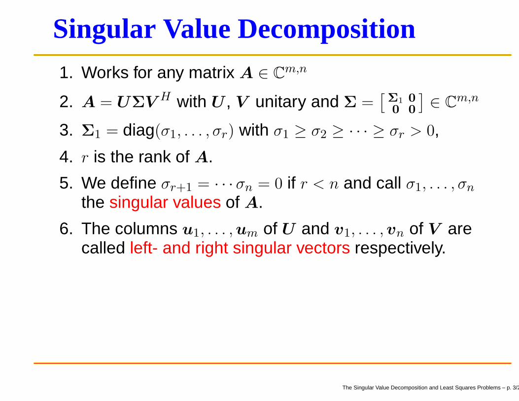
Singular Value Decomposition1. Works for any matrix A ∈ C

m,n

2. A = UΣV H with U , V unitary and Σ =[

Σ1 0

0 0

]

∈ Cm,n

3. Σ1 = diag(σ1, . . . , σr) with σ1 ≥ σ2 ≥ · · · ≥ σr > 0,

4. r is the rank of A.

5. We define σr+1 = · · · σn = 0 if r < n and call σ1, . . . , σn

the singular values of A.

6. The columns u1, . . . ,um of U and v1, . . . ,vn of V arecalled left- and right singular vectors respectively.


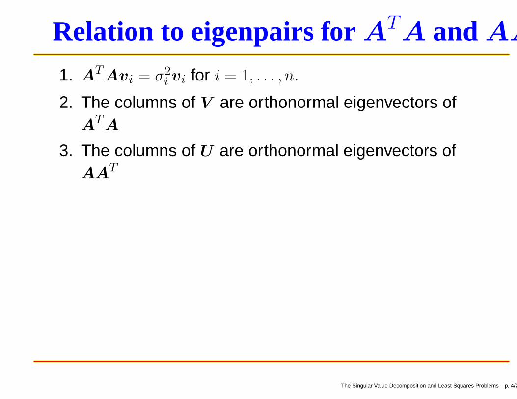
Relation to eigenpairs for ATA and AA

1. ATAvi = σ2i vi for i = 1, . . . , n.

2. The columns of V are orthonormal eigenvectors ofATA

3. The columns of U are orthonormal eigenvectors ofAAT


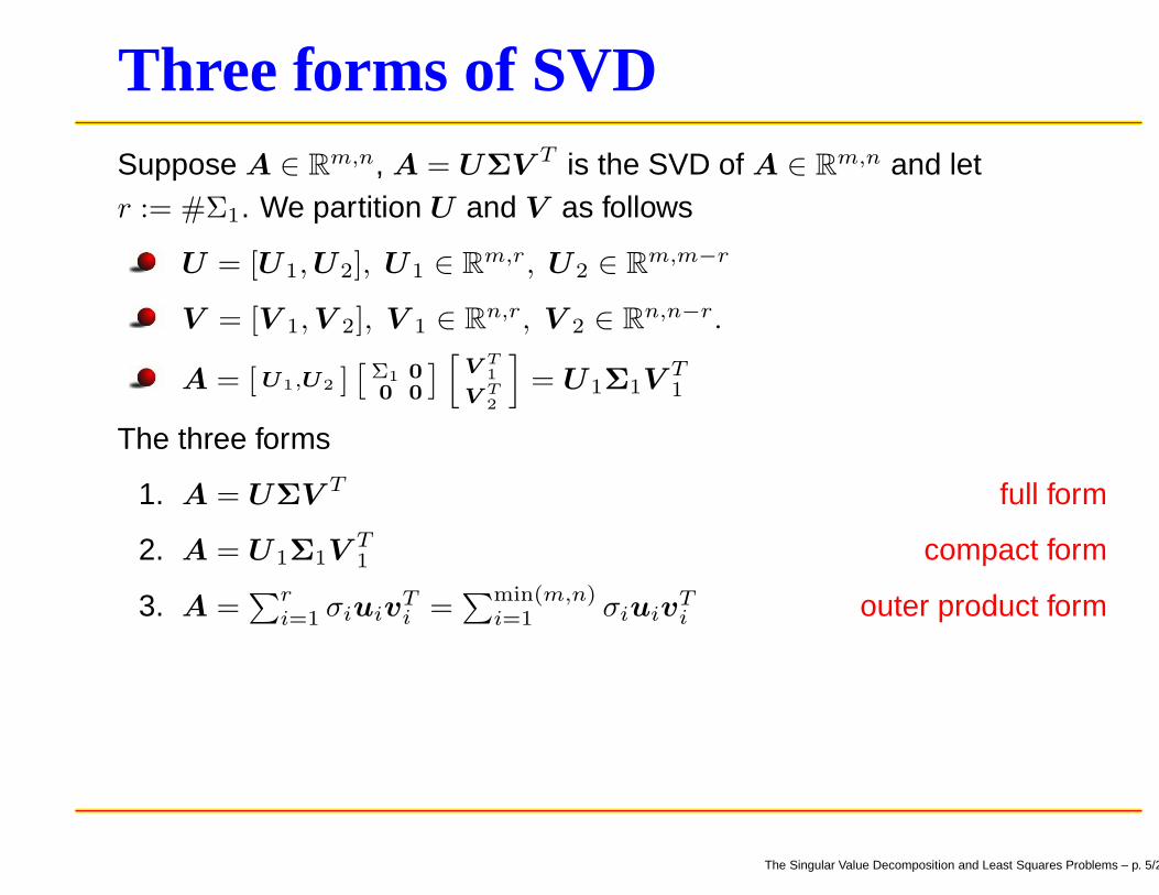
Three forms of SVDSuppose A ∈ Rm,n, A = UΣV T is the SVD of A ∈ Rm,n and letr := #Σ1. We partition U and V as follows

U = [U1, U2], U1 ∈ Rm,r, U2 ∈ R

m,m−r

V = [V 1, V 2], V 1 ∈ Rn,r, V 2 ∈ R

n,n−r.

A = [ U1,U2 ][

Σ1 0

0 0

]

[

VT

1

VT

2

]

= U1Σ1VT1

The three forms

1. A = UΣV T full form

2. A = U1Σ1VT1 compact form

3. A =∑r

i=1 σiuivTi =

∑min(m,n)i=1 σiuiv

Ti outer product form


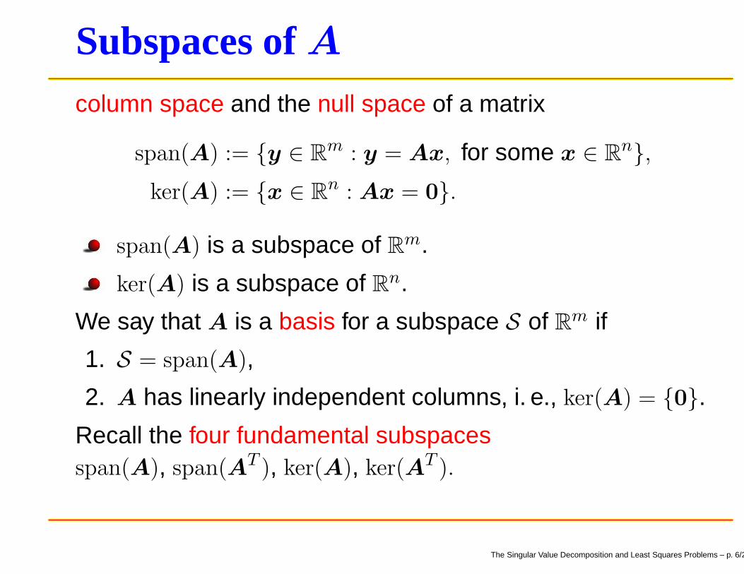
Subspaces of A

column space and the null space of a matrix

span(A) := {y ∈ Rm : y = Ax, for some x ∈ R

n},

ker(A) := {x ∈ Rn : Ax = 0}.

span(A) is a subspace of Rm.

ker(A) is a subspace of Rn.

We say that A is a basis for a subspace S of Rm if

1. S = span(A),

2. A has linearly independent columns, i. e., ker(A) = {0}.

Recall the four fundamental subspacesspan(A), span(AT ), ker(A), ker(AT ).


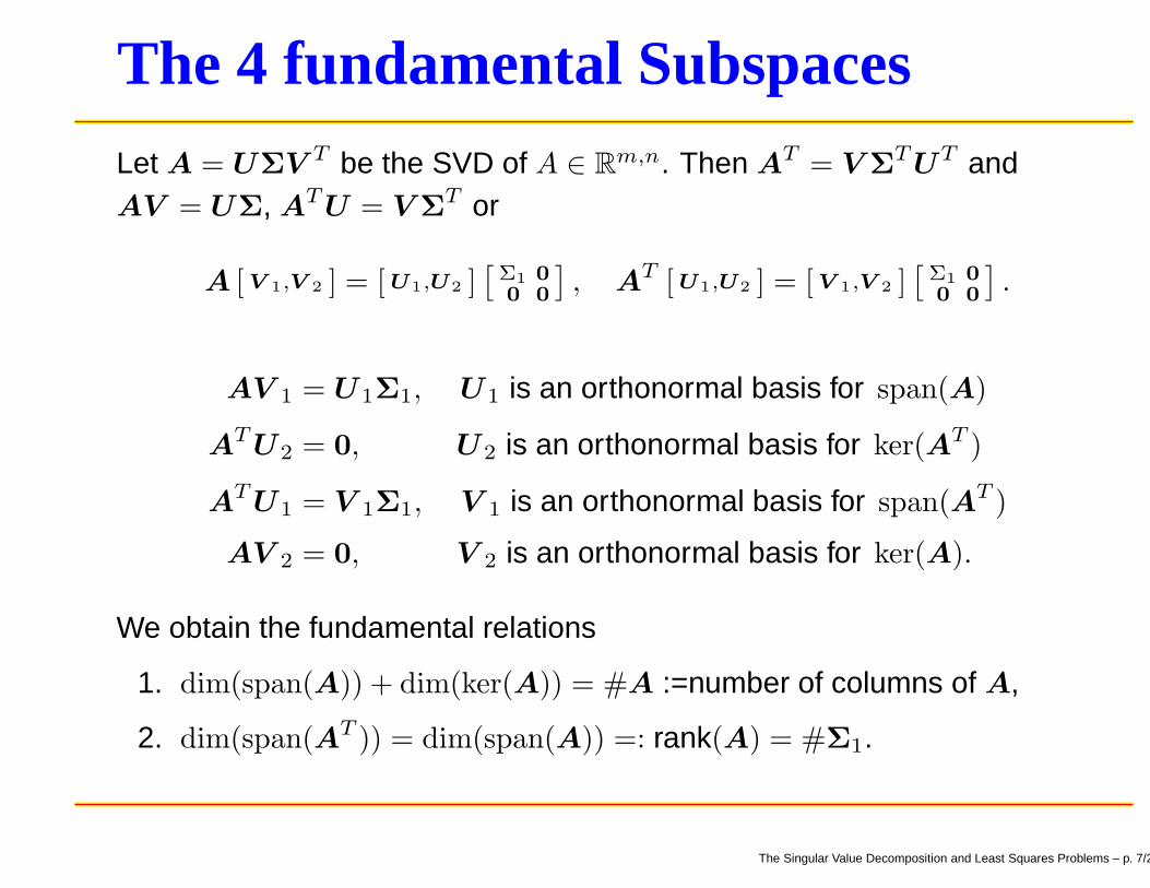
The 4 fundamental SubspacesLet A = UΣV T be the SVD of A ∈ Rm,n. Then AT = V Σ

T UT andAV = UΣ, AT U = V Σ

T or

A [ V 1,V 2 ] = [ U1,U2 ][

Σ1 0

0 0

]

, AT [ U1,U2 ] = [ V 1,V 2 ][

Σ1 0

0 0

]

.

AV 1 = U1Σ1, U1 is an orthonormal basis for span(A)

AT U2 = 0, U2 is an orthonormal basis for ker(AT )

AT U1 = V 1Σ1, V 1 is an orthonormal basis for span(AT )

AV 2 = 0, V 2 is an orthonormal basis for ker(A).

We obtain the fundamental relations

1. dim(span(A)) + dim(ker(A)) = #A :=number of columns of A,

2. dim(span(AT )) = dim(span(A)) =: rank(A) = #Σ1.


Existence of SVDTheorem 1. Every matrix has an SVD.


Uniqueness

If the SVD of A is A = UΣV T then ATA = V ΣTΣV T .

Thus σ21, . . . σ

2n are uniquely given as the eigenvalues of

ATA arranged in descending order.

Taking the positive square root uniquely determines thesingular values.

From the proof of the existence theorem it follows thatthe orthogonal matrices U and V are in general notuniquely given.


Application I, rankGauss-Jordan cannot be used to determine ranknumerically

Use singular value decomposition

numerically will normally find σn > 0.

Determine minimal r so that σr+1, . . . , σn are "close" toround off unit.


Application II, overdetermined EquationsGiven Am,n and b ∈ R

m.

The system Ax = b is over-determined if m > n.

This system has a solution if b ∈ span(A), the column space of A,but normally this is not the case and we can only find an approximatesolution.

A general approach is to choose a vector norm ‖·‖ and find x whichminimizes ‖Ax − b‖.

We will only consider the Euclidian norm here.


The Least Squares ProblemGiven Am,n and b ∈ R

m with m ≥ n ≥ 1. The problem to find x ∈ Rn

that minimizes ‖Ax − b‖2 is called the least squares problem.

A minimizing vector x is called a least squares solution of Ax = b.

Several ways to analyze:

Quadratic minimization

Orthogonal Projections

SVD


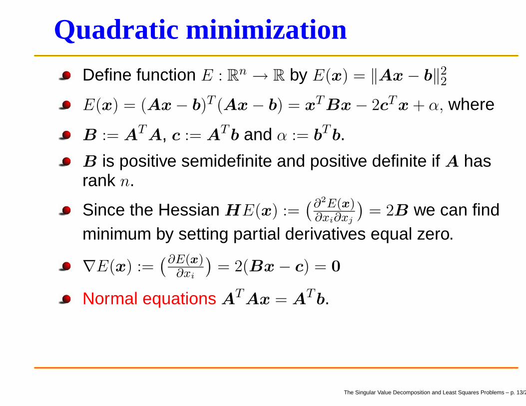
Quadratic minimization

Define function E : Rn → R by E(x) = ‖Ax − b‖2

2

E(x) = (Ax − b)T (Ax − b) = xT Bx − 2cT x + α, where

B := AT A, c := AT b and α := bT b.

B is positive semidefinite and positive definite if A hasrank n.

Since the Hessian HE(x) :=(∂2E(x)

∂xi∂xj

)

= 2B we can findminimum by setting partial derivatives equal zero.

∇E(x) :=(∂E(x)

∂xi

)

= 2(Bx − c) = 0

Normal equations AT Ax = ATb.


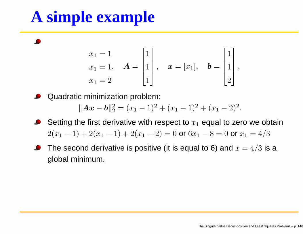
A simple example

x1 = 1

x1 = 1

x1 = 2

, A =

1

1

1

, x = [x1], b =

1

1

2

,

Quadratic minimization problem:‖Ax − b‖2

2 = (x1 − 1)2 + (x1 − 1)2 + (x1 − 2)2.

Setting the first derivative with respect to x1 equal to zero we obtain2(x1 − 1) + 2(x1 − 1) + 2(x1 − 2) = 0 or 6x1 − 8 = 0 or x1 = 4/3

The second derivative is positive (it is equal to 6) and x = 4/3 is aglobal minimum.


Theory; Direct sum and Orthogonal SumSuppose S and T are subspaces of a vector space (V , F). We define

1. Sum: X := S + T := {s + t : s ∈ S and t ∈ T };

2. Direct Sum: If S ∩ T = {0}, then S ⊕ T := S + T .

3. Orthogonal Sum: Suppose (V , F, 〈·, ·〉) is an inner product space.Then S ⊕ T is an orthogonal sum if 〈s, t〉 = 0 for all s ∈ S and allt ∈ T .

4. orthogonal complement:T = S⊥ := {x ∈ X : 〈s, x〉 = 0 for all s ∈ S}.


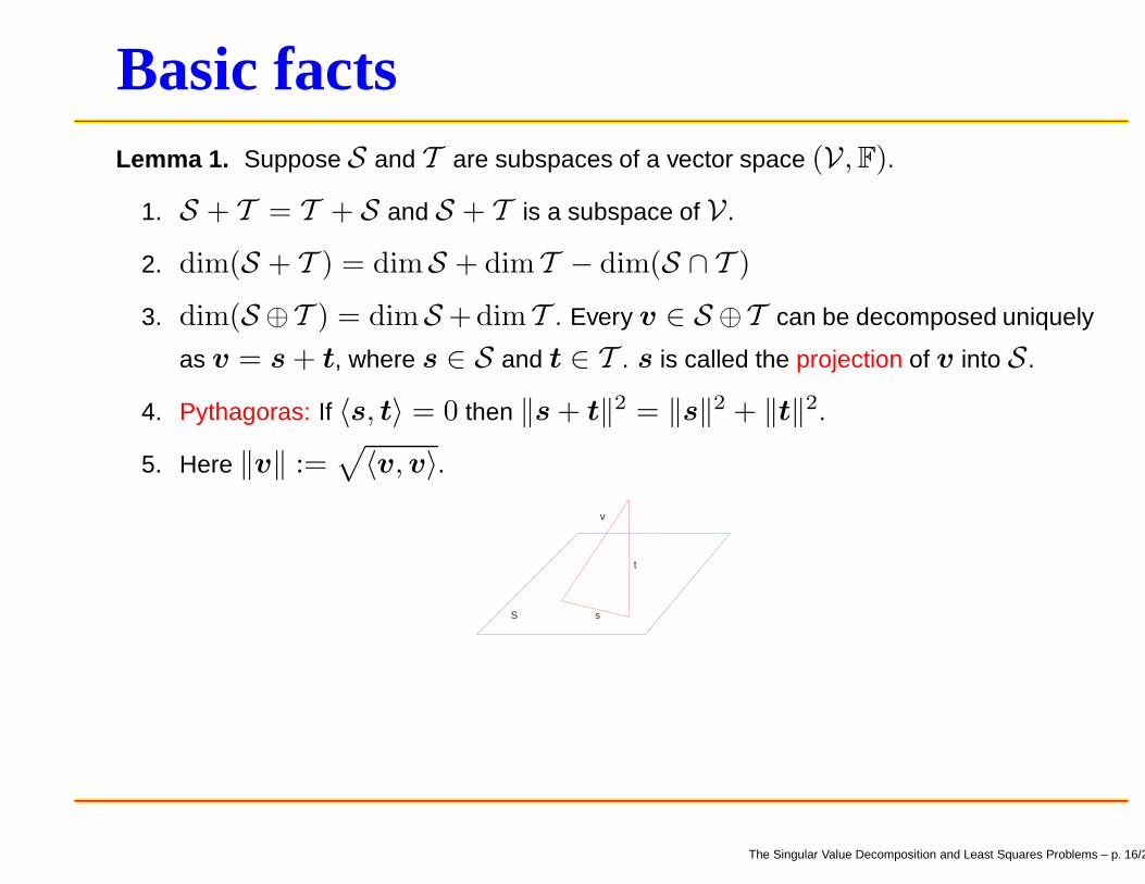
Basic factsLemma 1. Suppose S and T are subspaces of a vector space (V , F).

1. S + T = T + S and S + T is a subspace of V .

2. dim(S + T ) = dimS + dim T − dim(S ∩ T )

3. dim(S ⊕T ) = dimS +dimT . Every v ∈ S ⊕T can be decomposed uniquely

as v = s + t, where s ∈ S and t ∈ T . s is called the projection of v into S .

4. Pythagoras: If 〈s, t〉 = 0 then ‖s + t‖2 = ‖s‖2 + ‖t‖2.

5. Here ‖v‖ :=√

〈v, v〉.

v

t

sS


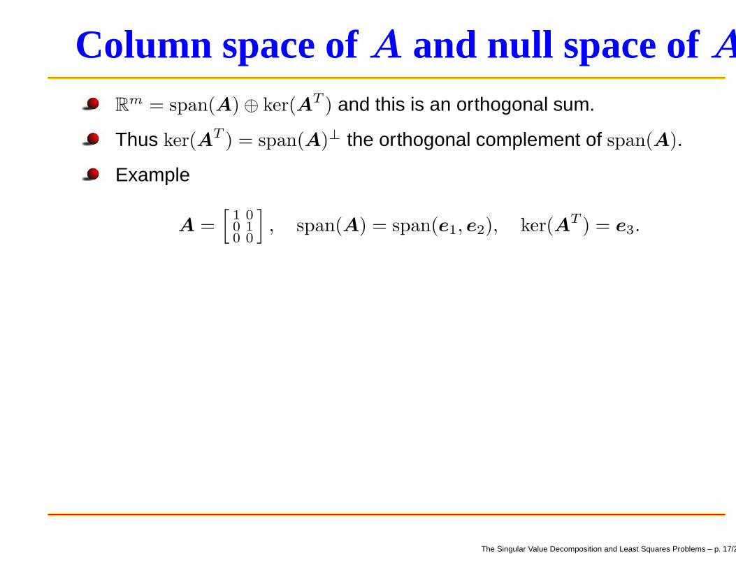
Column space of A and null space of A

Rm = span(A) ⊕ ker(AT ) and this is an orthogonal sum.

Thus ker(AT ) = span(A)⊥ the orthogonal complement of span(A).

Example

A =[

1 00 10 0

]

, span(A) = span(e1, e2), ker(AT ) = e3.


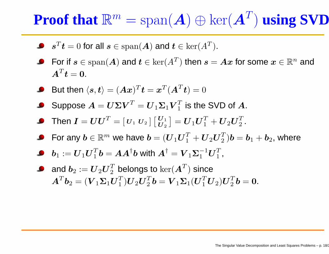
Proof that Rm = span(A) ⊕ ker(AT ) using SVD

sT t = 0 for all s ∈ span(A) and t ∈ ker(AT ).

For if s ∈ span(A) and t ∈ ker(AT ) then s = Ax for some x ∈ Rn and

AT t = 0.

But then 〈s, t〉 = (Ax)T t = xT (AT t) = 0

Suppose A = UΣV T = U1Σ1VT1 is the SVD of A.

Then I = UUT = [ U1 U2 ][

U1

U2

]

= U1UT1 + U2U

T2 .

For any b ∈ Rm we have b = (U1U

T1 + U2U

T2 )b = b1 + b2, where

b1 := U1UT1 b = AA†b with A† = V 1Σ

−11 UT

1 ,

and b2 := U2UT2 belongs to ker(AT ) since

AT b2 = (V 1Σ1UT1 )U2U

T2 b = V 1Σ1(U

T1 U2)U

T2 b = 0.


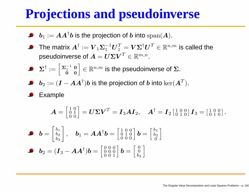
Projections and pseudoinverseb1 := AA†b is the projection of b into span(A).

The matrix A† := V 1Σ−11 UT

1 = V Σ†UT ∈ Rn,m is called the

pseudoinverse of A = UΣV T ∈ Rm,n.

Σ† :=

[

Σ−1

10

0 0

]

∈ Rn,m is the pseudoinverse of Σ.

b2 := (I − AA†)b is the projection of b into ker(AT ).

Example

A =[

1 00 10 0

]

= UΣV T = I3AI2, A† = I2 [ 1 0 00 1 0 ] I3 = [ 1 0 0

0 1 0 ] .

b =

[

b1

b2

b3

]

, b1 = AA†b =[

1 0 00 1 00 0 0

]

b =[

b1

b2

0

]

b2 = (I3 − AA†)b =[

0 0 00 0 00 0 1

]

b =[

00b3

]


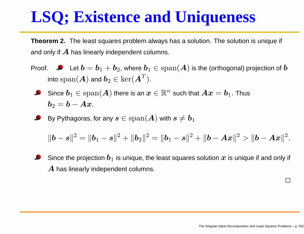
LSQ; Existence and UniquenessTheorem 2. The least squares problem always has a solution. The solution is unique if

and only if A has linearly independent columns.

Proof. Let b = b1 + b2, where b1 ∈ span(A) is the (orthogonal) projection of b

into span(A) and b2 ∈ ker(AT ).

Since b1 ∈ span(A) there is an x ∈ Rn such that Ax = b1. Thus

b2 = b − Ax.

By Pythagoras, for any s ∈ span(A) with s 6= b1

‖b − s‖2 = ‖b1 − s‖2 + ‖b2‖2 = ‖b1 − s‖2 + ‖b − Ax‖2 > ‖b − Ax‖2.

Since the projection b1 is unique, the least squares solution x is unique if and only if

A has linearly independent columns.


The Normal EquationsTheorem 3. Any solution x of the least squares problem is a solution of the linear system

AT Ax = AT b.

The system is nonsingular if and only if A has linearly independent columns.

Proof. Since b − Ax ∈ ker(AT ), we have AT (b − Ax) = 0 or

AT Ax = AT b.

AT A is nonsingular. Suppose AT Ax = 0 for some x ∈ Rn. Then

0 = xT AT Ax = (Ax)T Ax = ‖Ax‖22. Hence Ax = 0 which implies that

x = 0 if and only if A has linearly independent columns.

The linear system AT Ax = AT b is called the normal equations.


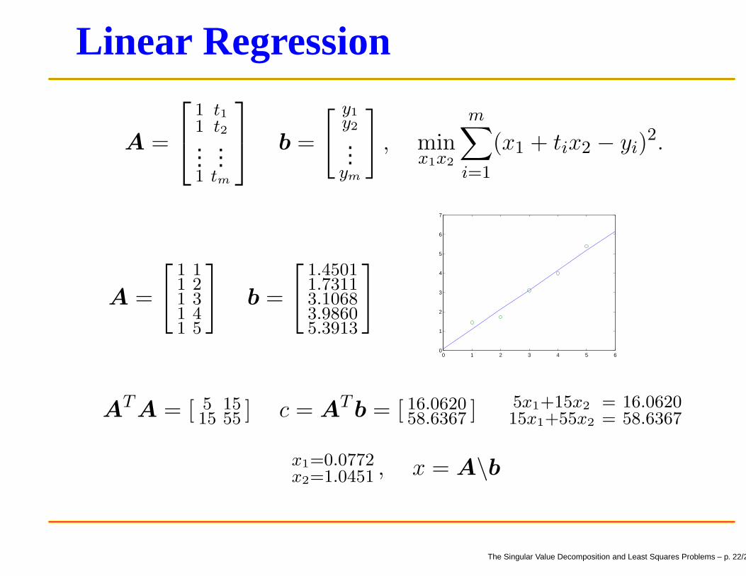
Linear Regression

A =

1 t11 t2...

...1 tm

b =

[ y1

y2

...ym

]

, minx1x2

m∑

i=1

(x1 + tix2 − yi)2.

A =

[

1 11 21 31 41 5

]

b =

[

1.45011.73113.10683.98605.3913

]

0 1 2 3 4 5 60

1

2

3

4

5

6

7

AT A = [ 5 1515 55 ] c = AT b = [ 16.0620

58.6367 ] 5x1+15x2 = 16.062015x1+55x2 = 58.6367

x1=0.0772x2=1.0451 , x = A\b


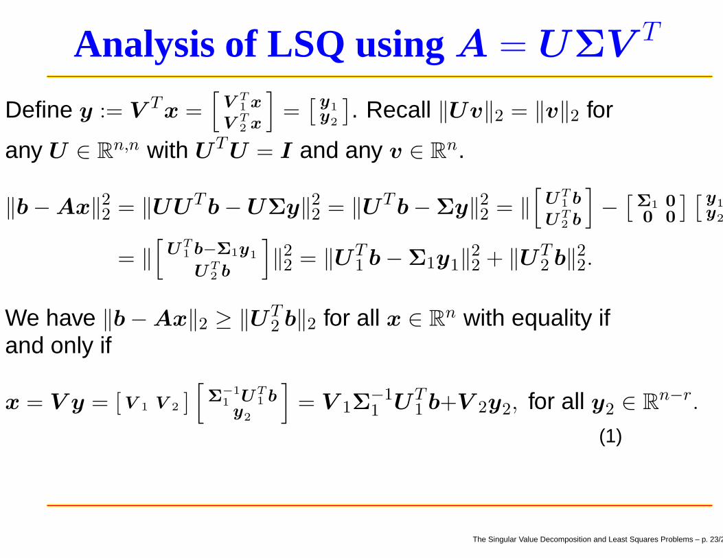
Analysis of LSQ using A = UΣV T

Define y := V Tx =[

V T1 x

V T2 x

]

=[ y

1

y2

]

. Recall ‖Uv‖2 = ‖v‖2 for

any U ∈ Rn,n with UT U = I and any v ∈ R

n.

‖b − Ax‖22 = ‖UUTb − UΣy‖2

2 = ‖UT b − Σy‖22 = ‖

[

UT1 b

UT2 b

]

−[

Σ1 0

0 0

] [ y1

y2

= ‖[

UT1 b−Σ1y1

UT2 b

]

‖22 = ‖UT

1 b − Σ1y1‖22 + ‖UT

2 b‖22.

We have ‖b − Ax‖2 ≥ ‖UT2 b‖2 for all x ∈ R

n with equality ifand only if

x = V y = [ V 1 V 2 ][

Σ−1

1UT

1 by

2

]

= V 1Σ−11 UT

1 b+V 2y2, for all y2 ∈ Rn−r.

(1)


The general solution of min‖Ax − b‖2

The columns of V 2 is a basis for ker(A) so thatker(A) = {z = V 2y2 : y2 ∈ R

n−r}.

Therefore the solution set is

{x ∈ Rn : ‖Ax − b‖2 is minimized } = A†b + ker(A).

If r = n then A has linearly independent columns andATA is nonsingular.

Since AT Ax = AT b we obtain A† = (ATA)−1AT in thiscase.


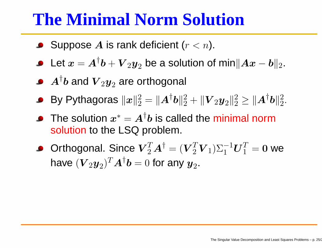
The Minimal Norm SolutionSuppose A is rank deficient (r < n).

Let x = A†b + V 2y2 be a solution of min‖Ax − b‖2.

A†b and V 2y2 are orthogonal

By Pythagoras ‖x‖22 = ‖A†b‖2

2 + ‖V 2y2‖22 ≥ ‖A†b‖2

2.

The solution x∗ = A†b is called the minimal normsolution to the LSQ problem.

Orthogonal. Since V T2 A† = (V T

2 V 1)Σ−11 UT

1 = 0 wehave (V 2y2)

T A†b = 0 for any y2.


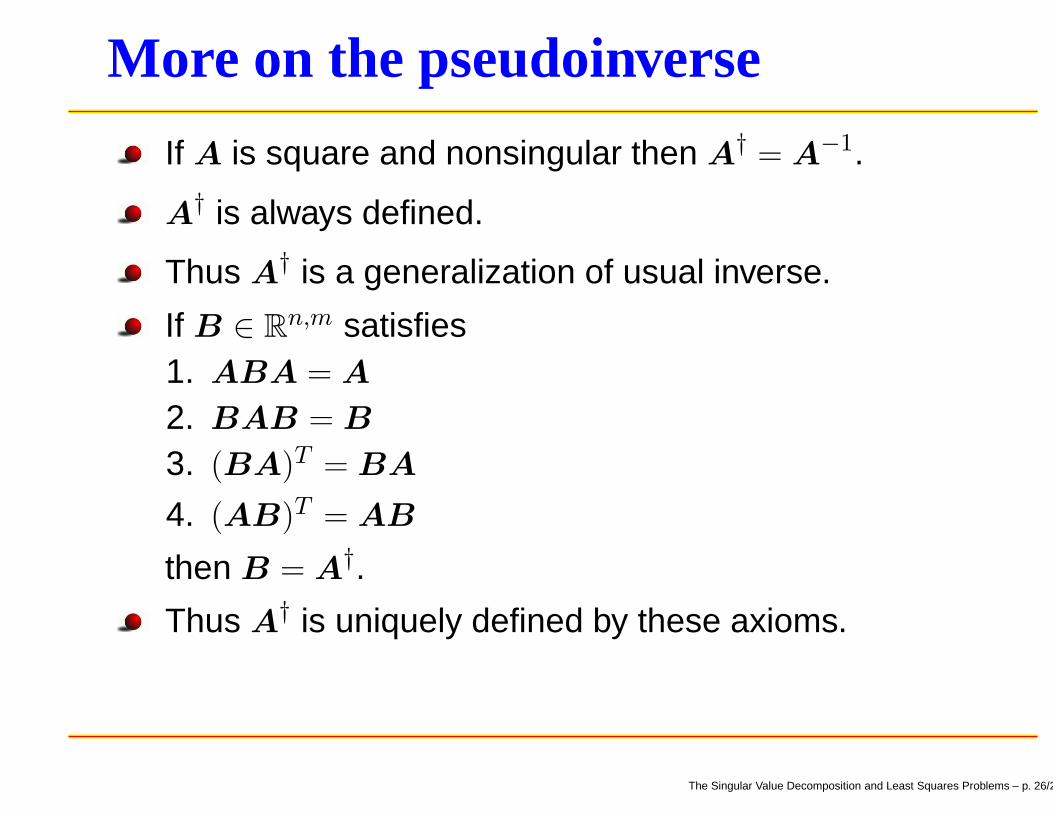
More on the pseudoinverse

If A is square and nonsingular then A† = A−1.

A† is always defined.

Thus A† is a generalization of usual inverse.

If B ∈ Rn,m satisfies

1. ABA = A

2. BAB = B

3. (BA)T = BA

4. (AB)T = AB

then B = A†.

Thus A† is uniquely defined by these axioms.


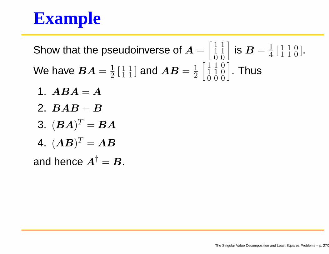
Example

Show that the pseudoinverse of A =[

1 11 10 0

]

is B = 14 [ 1 1 0

1 1 0 ].

We have BA = 12 [ 1 1

1 1 ] and AB = 12

[

1 1 01 1 00 0 0

]

. Thus

1. ABA = A

2. BAB = B

3. (BA)T = BA

4. (AB)T = AB

and hence A† = B.


the singular value decomposition and least squares problems · the singular value decomposition and...

Documents