the slip algorithm with a single iterationyuba.stanford.edu/~nickm/papers/nickmckeown_part3.pdfthe...
TRANSCRIPT
18
CHAPTER 2
The SLIP Algorithm
with a Single Iteration
1 Introduction
In this chapter we introduce, describe and evaluate the SLIP algorithm — a novel algorithm
for scheduling cells in input-queued switches. This chapter concentrates on the behavior of SLIP
with just a single iteration per cell time. In the next chapter we consider SLIP with multiple itera-
tions.
The SLIP algorithm uses rotating priority (“round-robin”) arbitration to schedule each active
input and output in turn. The main characteristic of SLIP is its simplicity: it is readily implemented
in hardware and can operate at high speed.
Before describing SLIP, we begin this chapter with a description of the basic round-robin
matching (RRM) algorithm. We show that RRM performs poorly and demonstrate this with some
examples. In Section 3 we introduce the SLIP algorithm as a variation of RRM. We show that the
performance of SLIP for uniform traffic is surprisingly good; in fact, for uniform i.i.d. Bernoulli
arrivals, SLIP with a single iteration is stable for any admissible load. This is the result of a phe-
nomenon that we encounter repeatedly in this chapter: the arbiters in SLIP have a tendency to
desynchronize with respect to one another.

CHAPTER 2 The SLIP Algorithm with a Single Iteration 19
As was observed for themaxsizealgorithm in Chapter 1, SLIP can become unstable for admis-
sible non-uniform traffic. In Section 5 we illustrate this with a 2x2 switch. For non-uniform i.i.d.
Bernoulli arrivals we find offered loads for which SLIP performsworse than themaxsizealgo-
rithm and offered loads for which SLIP performsbetter. We examine in detail a region of opera-
tion in which SLIP behaves non-monotonically: increasing offered load can actually decrease the
average queueing delay. We develop an analytical model describing this behavior, based on a sim-
plified version of the switch. We expand this model in Section 5.4 to analyze the delay perfor-
mance of a 2x2 SLIP switch.
In Section 6 we propose some variations on the basic SLIP algorithm, suitable for a number of
different applications. Finally, in Section 7 we describe the implementation of a centralized SLIP
scheduler, arguing that with current technology it is feasible to implement a 32x32 port scheduler
on a single chip.
CHAPTER 2 The SLIP Algorithm with a Single Iteration 20
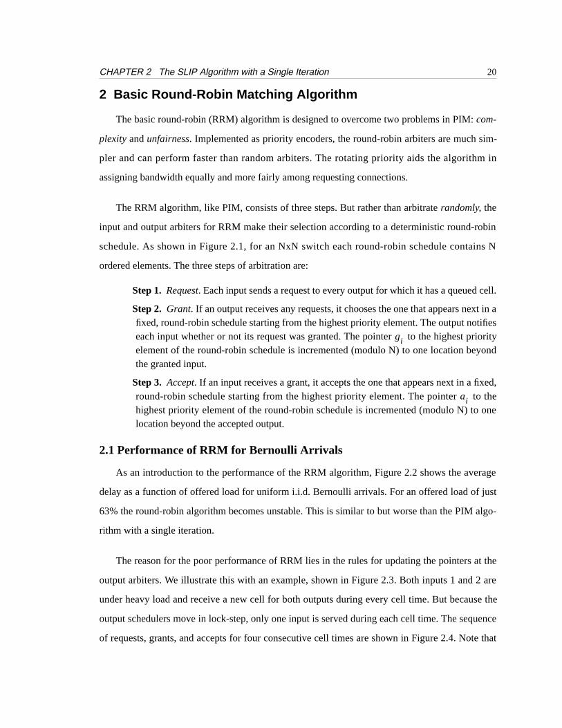
2 Basic Round-Robin Matching Algorithm
The basic round-robin (RRM) algorithm is designed to overcome two problems in PIM:com-
plexity andunfairness. Implemented as priority encoders, the round-robin arbiters are much sim-
pler and can perform faster than random arbiters. The rotating priority aids the algorithm in
assigning bandwidth equally and more fairly among requesting connections.
The RRM algorithm, like PIM, consists of three steps. But rather than arbitraterandomly, the
input and output arbiters for RRM make their selection according to a deterministic round-robin
schedule. As shown in Figure 2.1, for an NxN switch each round-robin schedule contains N
ordered elements. The three steps of arbitration are:
Step 1. Request. Each input sends a request to every output for which it has a queued cell.
Step 2. Grant. If an output receives any requests, it chooses the one that appears next in afixed, round-robin schedule starting from the highest priority element. The output notifieseach input whether or not its request was granted. The pointer to the highest priorityelement of the round-robin schedule is incremented (modulo N) to one location beyondthe granted input.
Step 3. Accept. If an input receives a grant, it accepts the one that appears next in a fixed,round-robin schedule starting from the highest priority element. The pointer to thehighest priority element of the round-robin schedule is incremented (modulo N) to onelocation beyond the accepted output.
2.1 Performance of RRM for Bernoulli Arrivals
As an introduction to the performance of the RRM algorithm, Figure 2.2 shows the average
delay as a function of offered load for uniform i.i.d. Bernoulli arrivals. For an offered load of just
63% the round-robin algorithm becomes unstable. This is similar to but worse than the PIM algo-
rithm with a single iteration.
The reason for the poor performance of RRM lies in the rules for updating the pointers at the
output arbiters. We illustrate this with an example, shown in Figure 2.3. Both inputs 1 and 2 are
under heavy load and receive a new cell for both outputs during every cell time. But because the
output schedulers move in lock-step, only one input is served during each cell time. The sequence
of requests, grants, and accepts for four consecutive cell times are shown in Figure 2.4. Note that
gi
ai
CHAPTER 2 The SLIP Algorithm with a Single Iteration 21
the grant pointers change in lock-step: in cell time 1 both point to input 1 and during cell time 2
both point to input 2etc. This synchronization phenomenon leads to a maximum throughput of
just 50%.
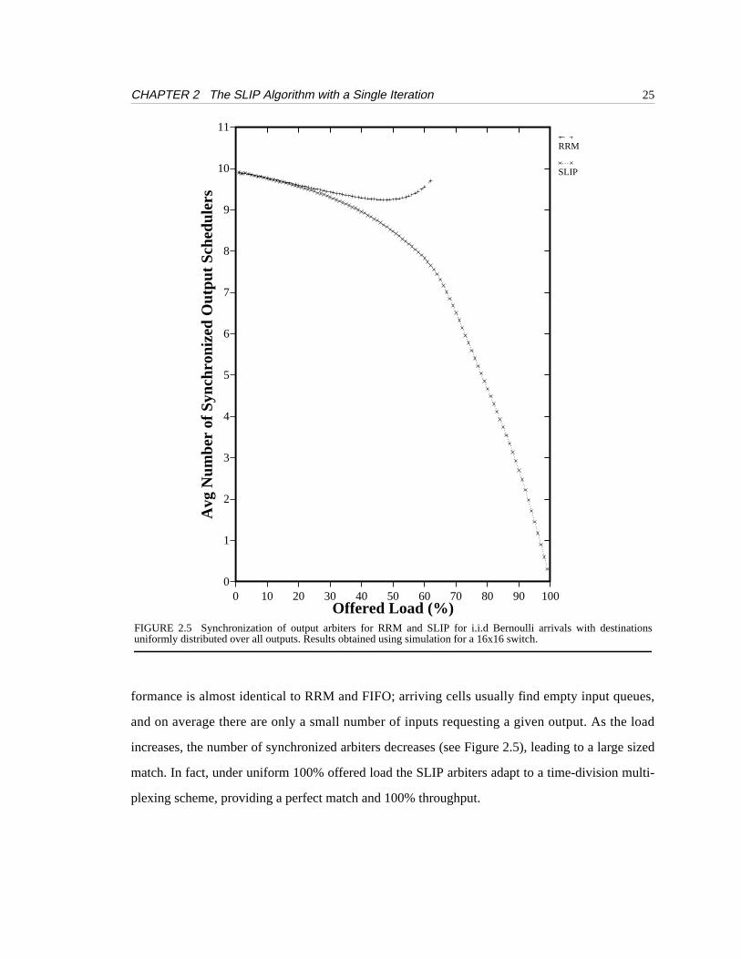
As an example of the effect of synchronization under a random arrival pattern, Figure 2.5
shows the number of synchronized output arbiters as a function of offered load for a 16x16 switch
with i.i.d Bernoulli arrivals. The graph plots the number of non-uniquegi’s, i.e. the number of out-
1
22
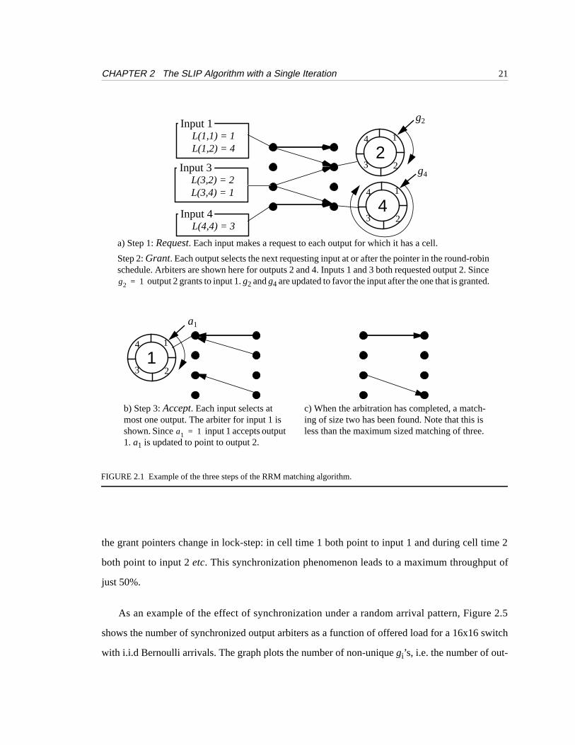
a) Step 1:Request. Each input makes a request to each output for which it has a cell.
Step 2:Grant. Each output selects the next requesting input at or after the pointer in the round-robinschedule. Arbiters are shown here for outputs 2 and 4. Inputs 1 and 3 both requested output 2. Since
output 2 grants to input 1.g2 andg4 are updated to favor the input after the one that is granted.g2 1=
Input 1L(1,1) = 1L(1,2) = 4
Input 3L(3,2) = 2L(3,4) = 1
Input 4L(4,4) = 3
c) When the arbitration has completed, a match-ing of size two has been found. Note that this isless than the maximum sized matching of three.
b) Step 3:Accept. Each input selects atmost one output. The arbiter for input 1 isshown. Since input 1 accepts output1. a1 is updated to point to output 2.
a1 1=
3
4
1
24
3
4
1
21
3
4
g2
g4
a1
FIGURE 2.1 Example of the three steps of the RRM matching algorithm.

CHAPTER 2 The SLIP Algorithm with a Single Iteration 22
put arbiters that clash with another arbiter. Under low offered load cells arriving for outputj will
find gj in a random position, equally likely to grant to any input. The probability that for all
is which for N=16 implies that the expected number of arbiters with the same
highest-priority value is 9.9. This agrees well with the simulation result for RRM in Figure 2.5. As
the offered load increases, synchronized output arbiters tend to move in lock-step and the degree
of synchronization changes only slightly.
FIGURE 2.2 Performance of RRM and SLIP compared with PIM for i.i.d Bernoulli arrivals with destinationsuniformly distributed over all outputs. Results obtained using simulation for a 16x16 switch. The graph shows theaverage delay per cell, measured in cell times, between arriving at the input buffers and departing from the switch.
30 40 50 60 70 80 9021 990.1
1
10
100
1e+03
Offered Load (%)
Avg
Cel
l Lat
ency
(C
ells
)
FIFO
PIM 1
RRM
SLIP
gj gk≠
k j≠ N 1–N
------------- N 1–

CHAPTER 2 The SLIP Algorithm with a Single Iteration 23
3 The SLIP Algorithm
The SLIP algorithm is a variation on RRM designed to reduce the synchronization of the out-
put arbiters. SLIP achieves this by not moving the grant pointers unless the grant is accepted lead-
ing to a desynchronization of the arbiters under high load. SLIP is identical to RRM except for a
condition placed on updating the grant pointers. TheGrant step of RRM is changed to:
Step 2. Grant. If an output receives any requests, it chooses the one that appears next in afixed, round-robin schedule starting from the highest priority element. The output notifieseach input whether or not its request was granted.The pointer to the highest priorityelement of the round-robin schedule is incremented (modulo N) to one location beyondthe granted input if and only if the grant is accepted in Step 3.
This small change to the algorithm leads to the following properties of SLIP:
Property 1. Lowest priority is given to the most recently made connection. This isbecause when the arbiters move their pointers, the most recently granted (accepted) input(output) becomes the lowest priority at that output (input). If inputi successfully connectsto outputj, bothai andgj are updated and the connection from inputi to outputj becomesthe lowest priority connection in the next cell time.
Property 2. No connection is starved. This is because an input will continue to request anoutput until it is successful. The output will serve at most N-1 other inputs first, waiting atmost N cell times to be accepted by each input. Therefore, a requesting input is alwaysserved in less than N2 cell times.
Property 3. Under heavy load, all queues with a common output have the same through-put. This is a consequence of Property 2: the output pointer moves to each requestinginput in a fixed order, thus providing each with the same throughput.
λ1 1, λ1 2, 1= =
λ2 1, λ2 2, 1= =
µ1 1, µ1 2, 0.25= =
µ2 1, µ2 2, 0.25= =
FIGURE 2.3 2x2 switch with RRM algorithm under heavy load. Synchronization of output arbiters leads to athroughput of just 50%.
gi

CHAPTER 2 The SLIP Algorithm with a Single Iteration 24
But most importantly, this small change prevents the output arbiters from moving in lock-step
leading to a dramatic improvement in performance.
4 Simulated Performance of SLIP
4.1 Bernoulli Traffic
To illustrate the improvement in performance of SLIP over RRM, Figure 2.2 shows the perfor-
mance of the two algorithms under uniform i.i.d. Bernoulli arrivals. Under low load, SLIP’s per-
g1
g2
are the grant pointers,a1
a2
are the accept pointers,
i1i2
R j1 j2j1 j2
means:Input 1 requests outputs 1 and 2
Input 2 requests outputs 1 and 2
j1j2
G i1i1
means:Output 1 grants to input 1
Output 2 grants to input 1
i1i2
A j2j1
means:Input 1 accepts output 2
Input 2 accepts output 1
Cell 1:g1
g2
1
1=
a1
a2
1
1=,
i1i2
R j1 j2j1 j2
j1j2
G i1i1
i1 A j1→ →
Cell 2:g1
g2
2
2=
a1
a2
2
1=,
i1i2
R j1 j2j1 j2
j1j2
G i2i2
i2 A j1→ →
Cell 3:g1
g2
1
1=
a1
a2
2
2=,
i1i2
R j1 j2j1 j2
j1j2
G i1i1
i1 A j2→ →
Cell 4:g1
g2
2
2=
a1
a2
1
2=,
i1i2
R j1 j2j1 j2
j1j2
G i1i1
i2 A j2→ →
FIGURE 2.4 Illustration of low throughput for RRM caused by synchronization of output arbiters. Note that pointers[gi] stay synchronized, leading to a maximum throughput of just 50%.
Key:
CHAPTER 2 The SLIP Algorithm with a Single Iteration 25
formance is almost identical to RRM and FIFO; arriving cells usually find empty input queues,
and on average there are only a small number of inputs requesting a given output. As the load
increases, the number of synchronized arbiters decreases (see Figure 2.5), leading to a large sized
match. In fact, under uniform 100% offered load the SLIP arbiters adapt to a time-division multi-
plexing scheme, providing a perfect match and 100% throughput.
FIGURE 2.5 Synchronization of output arbiters for RRM and SLIP for i.i.d Bernoulli arrivals with destinationsuniformly distributed over all outputs. Results obtained using simulation for a 16x16 switch.
0 10 20 30 40 50 60 70 80 90 1000
1
2
3
4
5
6
7
8
9
10
11
Offered Load (%)
Avg
Num
ber
of S
ynch
roni
zed
Out
put S
ched
uler
s
RRM
SLIP

CHAPTER 2 The SLIP Algorithm with a Single Iteration 26
Figure 2.6 is an example for a 2x2 switch showing how under heavy traffic the arbiters adapt
to an efficient time-division multiplexing schedule.
4.2 “Bursty” Traffic
Real network traffic is highly correlated from cell to cell [32] and so in practice, cells tend to
arrive in bursts, corresponding perhaps to a packet that has been segmented or a packetized video
frame. Many ways of modeling bursts in network traffic have been proposed [16], [21], [4], [32].
Recently, Lelandet al. [32] have demonstrated that measured network traffic is bursty at every
level making it important to understand the performance of switches in the presence of bursty traf-
fic.
We illustrate the effect of burstiness on SLIP using an on-off arrival process modulated by a 2-
state Markov-chain. The source alternately produces a burst of full cells (all with the same destina-
tion) followed by an idle period of empty cells. The bursts and idle periods contain a geometrically
distributed number of cells.
Figure 2.7 shows the performance of SLIP under this arrival process for a 16x16 switch, com-
paring it with the performance under uniform i.i.d. Bernoulli arrivals. As we would expect, the
FIGURE 2.6 Illustration of 100% throughput for SLIP caused by desynchronization of output arbiters. Note thatpointers [gi] become desynchronized at the end of Cell 1 and stay desynchronized, leading to an alternating cycle of 2cell times and a maximum throughput of 100%.
Cell 1:g1
g2
1
1=
a1
a2
1
1=,
i1i2
R j1 j2j1 j2
j1j2
G i1i1
i1 A j1→ →
Cell 2:g1
g2
2
1=
a1
a2
2
1=,
i1i2
R j1 j2j1 j2
j1j2
G i2i1
i1i2
A j2j1
→ →
Cell 3:g1
g2
1
2=
a1
a2
1
2=,
i1i2
R j1 j2j1 j2
j1j2
G i1i2
i1i2
A j1j2
→ →
Cell 4:g1
g2
2
1=
a1
a2
2
1=,
i1i2
R j1 j2j1 j2
j1j2
G i2i1
i1i2
A j2j1
→ →

CHAPTER 2 The SLIP Algorithm with a Single Iteration 27
increased burst size leads to a higher queueing delay. In fact, the average latency isproportional to
the expected burst length.
Although not shown here, we have also compared the performance of SLIP with other algo-
rithms for this traffic model. Our results suggest that for all the algorithms described in this thesis,
the increase in average queueing delay for input-queued switches is approximately proportional to
the expected burst length. In fact, the performance of the input-queued switch scheduling algo-
rithms become more and more alike and can become similar to the performance of an output-
FIGURE 2.7 The performance of SLIP under 2-state Markov-modulated Bernoulli arrivals. All cells within a burst aresent to the same output. Destinations of bursts are uniformly distributed over all outputs.
20 30 40 50 60 70 80 90 1000.1
1
10
100
1e+03
1e+04
1e+05
Offered Load (%)
Avg
Lat
ency
per
Cel
l (C
ells
)
Bernoulli
Burst=16
Burst=32
Burst=64
CHAPTER 2 The SLIP Algorithm with a Single Iteration 28
queued switch. This similarity indicates that the performance for bursty traffic is not heavily influ-
enced by the queueing policy. Burstiness tends to concentrate the conflicts on outputs rather than
inputs: each burst contains cells destined for the same output and each input will be dominated by
a single burst at a time. As a result, the performance is limited by output contention.
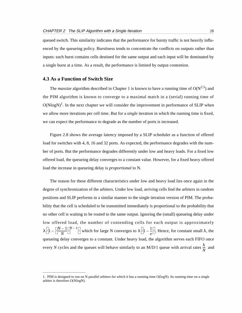
4.3 As a Function of Switch Size
Themaxsize algorithm described in Chapter 1 is known to have a running time of O(N2.5) and
the PIM algorithm is known to converge to a maximal match in a (serial) running time of
O(NlogN)1. In the next chapter we will consider the improvement in performance of SLIP when
we allow more iterations per cell time. But for asingle iteration in which the running time is fixed,
we can expect the performance to degrade as the number of ports is increased.
Figure 2.8 shows the average latency imposed by a SLIP scheduler as a function of offered
load for switches with 4, 8, 16 and 32 ports. As expected, the performance degrades with the num-
ber of ports. But the performance degrades differently under low and heavy loads. For a fixed low
offered load, the queueing delay converges to a constant value. However, for a fixed heavy offered
load the increase in queueing delay isproportional to N.
The reason for these different characteristics under low and heavy load lies once again in the
degree of synchronization of the arbiters. Under low load, arriving cells find the arbiters in random
positions and SLIP performs in a similar manner to the single iteration version of PIM. The proba-
bility that the cell is scheduled to be transmitted immediately is proportional to the probability that
no other cell is waiting to be routed to the same output. Ignoring the (small) queueing delay under
low offered load, the number of contending cells for each output is approximately
which for large N converges to . Hence, for constant smallλ, the
queueing delay converges to a constant. Under heavy load, the algorithm serves each FIFO once
everyN cycles and the queues will behave similarly to an M/D/1 queue with arrival rates and
1. PIM is designed to run on N parallel arbiters for which it has a running time O(logN). Its running time on a singlearbiter is therefore O(NlogN).
λ 1N 1–
N-------------
N 1––
λ 1 1e---–
λN----
CHAPTER 2 The SLIP Algorithm with a Single Iteration 29
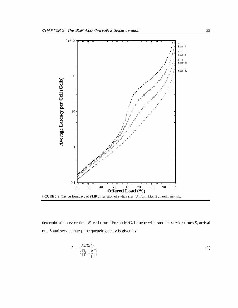
deterministic service time cell times. For an M/G/1 queue with random service timesS, arrival
rateλ and service rateµ the queueing delay is given by
. (1)
FIGURE 2.8 The performance of SLIP as function of switch size. Uniform i.i.d. Bernoulli arrivals.
30 40 50 60 70 80 9021 990.1
1
10
100
1e+03
Offered Load (%)
Ave
rage
Lat
ency
per
Cel
l (C
ells
)
Size=4
Size=8
Size=16
Size=32
N
dλE S2( )
2 1 λµ---–
----------------------=

CHAPTER 2 The SLIP Algorithm with a Single Iteration 30
So, for the SLIP switch under a heavy load of Bernoulli arrivals the delay will be approxi-
mately
(2)
which is proportional toN.
4.4 Burst Reduction
In Section 4.2 we saw the not surprising result that burstiness increases queueing delay. In
addition to the performance of a single switch for bursty traffic, it is important to consider the
effect that the switch has on other switches downstream. Intuitively, if a switch decreases the aver-
age burst length of traffic that it forwards, then we can expect it to improve the performance of its
downstream neighbor. We next examine the burst-reduction properties of SLIP.
There are many definitions of burstiness, for example the coefficient of variation [43], bursti-
ness curves [28], maximum burst length [7], or effective bandwidth [31]. In this section, we use
the same measure of burstiness that we used when generating traffic in Section 4.2: the average
burst length. We define a burst of cells at the output of a switch as the number of consecutive cells
that entered the switch at the same input.
SLIP is a deterministic algorithm, serving each connection in strict rotation. We therefore
expect that bursts of cells at different inputs contending for the same output will become inter-
leaved and the burstiness will be reduced. This is indeed the case, as shown in Figure 2.9. The
graph shows the average burst length at the switch output as a function of offered load. Arrivals
are on-off processes modulated by a 2-state Markov chain with average burst lengths of 16, 32 and
64 cells, as described in Section 4.2.
Our results indicate that SLIP reduces the average burst length, and will tend to be more burst-
reducing as the offered load increases. This is because the probability of switching between multi-
ple connections increases as the utilization increases. When the offered load is low, arriving bursts
do not encounter output contention and the burst of cells is passed unmodified. As the load
dλN
2 1 λ–( )----------------------=

CHAPTER 2 The SLIP Algorithm with a Single Iteration 31
increases, the contention increases and bursts are interleaved at the output. In fact, if the offered
load exceeds approximately 70%, the average burst length drops to exactly one cell. This indicates
that the output arbiters have become desynchronized and are operating as time-division multiplex-
ers, serving each input in turn.
FIGURE 2.9 Average burst length at switch output as a function of offered load. The arrivals are on-off processesmodulated by a 2-state DTMC. Results are for a 16x16 switch using the SLIP scheduling algorithm.
0 10 20 30 40 50 60 70 80 900
10
20
30
40
50
60
64
Offered Load (%)
Avg
Bur
st le
ngth
(C
ells
)
Burst=16
Burst=32
Burst=64
CHAPTER 2 The SLIP Algorithm with a Single Iteration 32
5 Analysis of SLIP Performance
In general, it is difficult to analyze the performance of a SLIP switch, even for the simplest
traffic models. Under uniform load and either very low or very high offered load we can readily
approximate and understand the way in which SLIP operates. When arrivals are infrequent we can
assume that the arbiters act independently and that arriving cells are successfully scheduled with
very low delay. At the other extreme, when the switch becomes uniformly backlogged, we can see
that desycnhronization will lead the arbiters to find an efficient time division multiplexing scheme
and operate without contention. But when the traffic is non-uniform, or when the offered load is at
neither extreme, the interaction between the arbiters becomes difficult to describe. The problem
lies in the evolution and interdependence of the state of each arbiter and their dependence on arriv-
ing traffic.
5.1 Convergence to Time-Division Multiplexing Under Heavy Load
In Section 4.3 we argued that under heavy load, SLIP will behave similarly to an M/D/1 queue
with arrival rates and deterministic service time cell times. So, under a heavy load of Ber-
noulli arrivals the delay will be approximated by Equation 2.
To see how close SLIP becomes to time-division multiplexing under heavy load, Figure 2.10
compares the average latency for both SLIP and an M/D/1 queue (Equation 2). Above an offered
load of approximately 70%, SLIP behaves very similarly to the M/D/1 queue, but with a higher
latency. This is because the service policy is not constant: when a queue changes between empty
and non-empty, the scheduler must adapt to the new set of queues that require service. This adap-
tion takes place over many cell times while the arbiters desynchronize again. During this time, the
throughput will be worse than for the M/D/1 queue and the queue length will increase. This in turn
will lead to an increased latency.
5.2 Desynchronization of Arbiters
We have argued that the performance of SLIP is dictated by the degree of synchronization of
the output schedulers. In this section we present a simple model of synchronization for a stationary
and sustainable uniform arrival process.
λN---- N

CHAPTER 2 The SLIP Algorithm with a Single Iteration 33
In Appendix 1 we find an approximation for , the expected number of synchronized
output schedulers at timet. The approximation is based on two assumptions:
1. Inputs that are unmatched at timet are uniformly distributed over all inputs.
2. The number of unmatched inputs at timet has zero variance.
This leads to the approximation
(3)
FIGURE 2.10 Comparison of average latency for the SLIP algorithm and an M/D/1 queue. The switch is 16x16 and,for the SLIP algorithm, arrivals are uniform i.i.d. Bernoulli arrivals.
20 30 40 50 60 70 80 90 990.1
1
10
100
1e+03
Offered Load (%)
Avg
Cel
l Lat
ency
(C
ells
)
SLIP
M/D/1
E S t( )[ ]
E S t( )[ ] N λNλN 1–
λN----------------
λλN– λ2NλN 1–
λN----------------
λ2N 1––≈

CHAPTER 2 The SLIP Algorithm with a Single Iteration 34
where,
This approximation is quite accurate over a wide range of uniform workloads. Figure 2.11
compares the approximation in Equation 3 with simulation results for both i.i.d. Bernoulli arrivals
and for an on-off arrival process modulated by a 2-state Markov-chain (described in Section 4.2).
N number of ports,=
λ arrival rate averaged over all inputs,=
λ 1 λ–( ) .=
0 10 20 30 40 50 60 70 80 90 1000
1
2
3
4
5
6
7
8
9
10
11
Offered Load (%)
Avg
Num
ber
of S
ynch
roni
zed
Out
put S
ched
uler
s
bernoulli_iid_uniform
train_64
Analytical
FIGURE 2.11 Comparison of analytical approximation and simulation results for the average number of synchronizedoutput schedulers. Simulation results are for a 16x16 switch with i.i.d Bernoulli arrivals and an on-off processmodulated by a 2-state Markov chain with an average burst length of 64 cells. The analytical approximation is shown inEquation 3.

CHAPTER 2 The SLIP Algorithm with a Single Iteration 35
5.3 Stability of SLIP
Figure 2.2 shows that the SLIP algorithm is stable for all admissible uniform i.i.d. Bernoulli
traffic. In practice, however, traffic tends to be concentrated among a small number of ports that
have quite asymmetric transmit and receive behavior, making the traffic non-uniform. In this sec-
tion we consider the stability of SLIP under non-uniform traffic.
In Chapter 1 we saw that a 2x2 switch can be unstable for the maximum sized matching algo-
rithm for admissible i.i.d. Bernoulli arrivals,when the traffic pattern is non-uniform. SLIP oper-
ates efficiently by mimicking the behavior of the maximum matching algorithm under heavy load.
It is therefore not surprising that a 2x2 switch using the SLIP algorithm can also be unstable under
non-uniform traffic.
We illustrate the region of instability for SLIP using the 2x2 switch shown in Figure 2.12.
With i.i.d. Bernoulli arrivals, we find that the SLIP algorithm is not only unstable for certain
arrival rates, but also that its behavior is non-monotonic: increasing the arrival rate can actually
reduce the expected occupancy of the input queues.
Figure 2.13(a) illustrates this surprising effect: fixing and varying
we see that SLIP becomes unstable in the region , but
becomes stable again for . It is also interesting to note that the behavior of
Q(1,2) and Q(2,1) is unaffected by Q(1,1), increasing monotonically even through the region of
instability for Q(1,1).
FIGURE 2.12 2x2 Switch with 3 active flows.
λ1 1,
λ1 2,
λ2 1,
µ1 1,
µ1 2,
µ2 1,
λ1 = λ1 1,( ) 0.48=
λ2 = λ1 2, = λ2 1,( ) 0.41 λ2 0.44≤ ≤
0.44 λ2 1 λ1–< <
CHAPTER 2 The SLIP Algorithm with a Single Iteration 36
In contrast,maxsize behaves quite differently: as shown in Figure 2.13(b) Q(1,1) becomes
unstable for all .
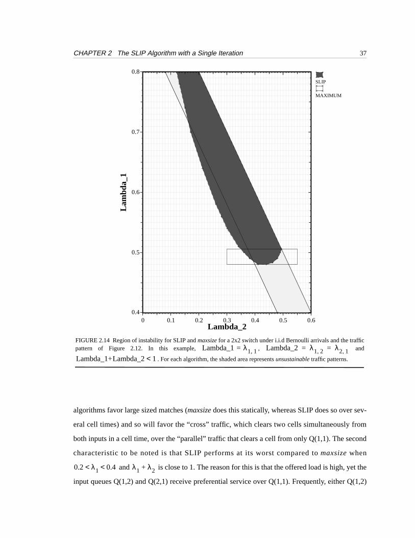
The region in which SLIP behaves non-monotonically is small. Figure 2.14 compares the
region of instability for both SLIP andmaxsize. Whereasmaxsizehas a stable region over most of
the region of admissible traffic bounded by , the region for SLIP is more complex.
Over most of the region of admissible traffic, increasingλ1 or λ2 cannot change SLIP from unsta-
ble to stable. However, this is not the case for , highlighted by the rectangle in
Figure 2.14.
Before trying to model this behavior, let us consider the intuition to be drawn from Figure
2.14. First, the region of instability is not symmetric in and : the switch is more susceptible
to instability for small when is large than vice-versa. This is also true formaxsize. Both
0.2 0.3 0.4 0.50.520.1
1
10
100
1e+03
Lambda_2
Avg
Que
ue O
ccup
ancy
, E[L
(i,j)]
(C
ells
)Q(1,1)
Q(1,2)
Q(2,1)
b) Maxsize algorithm.a) SLIP. Note that Q(1,1) becomes unstable
for , but is stable again as
traffic is increased.
0.41 λ≤ 2 0.44≤
FIGURE 2.13 Example of instability for SLIP and maximum sized matching algorithms for 2x2 switch. Traffic patternas shown in Figure 2.12, .λ1 0.48=
0.2 0.3 0.4 0.50.520.1
1
10
100
1e+03
Lambda_2
Q(1,1)
Q(1,2)
Q(2,1)
0.4 λ2 1 λ1–≤ ≤
λ1 λ2+ 0.88=
0.48 λ1 0.51≤ ≤
λ1 λ2
λ2 λ1
CHAPTER 2 The SLIP Algorithm with a Single Iteration 37
algorithms favor large sized matches (maxsize does this statically, whereas SLIP does so over sev-
eral cell times) and so will favor the “cross” traffic, which clears two cells simultaneously from
both inputs in a cell time, over the “parallel” traffic that clears a cell from only Q(1,1). The second
characteristic to be noted is that SLIP performs at its worst compared tomaxsize when
and is close to 1. The reason for this is that the offered load is high, yet the
input queues Q(1,2) and Q(2,1) receive preferential service over Q(1,1). Frequently, either Q(1,2)
FIGURE 2.14 Region of instability for SLIP andmaxsize for a 2x2 switch under i.i.d Bernoulli arrivals and the trafficpattern of Figure 2.12. In this example, , and
. For each algorithm, the shaded area representsunsustainable traffic patterns.
Lambda_1 λ= 1 1, Lambda_2 λ1 2, λ2 1,= =
Lambda_1+Lambda_2 1<
0 0.1 0.2 0.3 0.4 0.5 0.60.4
0.5
0.6
0.7
0.8
Lambda_2
Lam
bda_
1
SLIP
MAXIMUM
0.2 λ< 1 0.4< λ1 λ2+

CHAPTER 2 The SLIP Algorithm with a Single Iteration 38
or Q(2,1) will change between empty and non-empty, requiring SLIP to adapt to the new traffic
pattern. This inhibits the tendency of the arbiters to desynchronize.
5.3.1 Drift Analysis of a 2x2 SLIP Switch: First Approximation
To try and understand the non-monotonic behavior of SLIP, we examine the more tractable,
simplified switch with only one queue Q(1,1) shown in Figure 2.15. This switch behaves similarly
to the 2x2 switch with 3 queues in Figure 2.12, except that cells arriving at input 1 and destined for
output 2 are not queued. A cell arrives at the beginning of the time slot with probabilityε; if the
cell is not scheduled to be transmitted in the same cell time, it is discarded. Similarly for cells
arriving at input 2 destined for output 1.
In Appendix 2 Section 1 we analyze this switch to determine values ofλ and ε for which the
switch is unstable. By considering the expected increase in L, the occupancy of Q(1,1), at each cell
time, we find that the switch is unstable for
. (4)
This result is confirmed in Appendix 2 Section 2 where the distribution function for the occu-
pancy of Q(1,1) is found using the matrix geometric method of Neuts [36].
Equation 4 is plotted in Figure 2.16 along with the admissibility constraint . The area
between the curves is the region for which . Comparing Figure 2.16 with the
region of stability for the full 2x2 switch in Figure 2.14, we see that they are quite different.
λε
ε
FIGURE 2.15 Simplified 2x2 switch with a single queue, Q(1,1).
L
λ 1
1 2ε ε2 2ε3–+ +----------------------------------------->
λ ε 1<+
E L t( )[ ] ∞→

CHAPTER 2 The SLIP Algorithm with a Single Iteration 39
Although the model captures the asymmetry between and , and the fact that the switch per-
forms worst when is small and , it doesnot capture the non-monotonic behavior of
SLIP. In fact, we should expect the behavior to be different: cells that arrive at one of the unbuf-
fered inputs of our simplified switch can only affect the switch for a single cell time. Cells arriving
at the full 2x2 switch of Figure 2.12 that are unscheduled when they first arrive will still be there in
the next cell time, reducing the likelihood that Q(1,1) will be serviced.
We can substantially improve the accuracy of our model by estimating the number of cell
times that an arriving cell will affect the scheduling algorithm and increase the arrival rate,ε to
compensate.
Our claim is that the arrival rate in the approximate model should bedoubled,i.e. .
Our argument in support of this is a heuristic one: when a cell arrives at an empty queue in the
exact model, it is either successfully scheduled immediately or it is queued. If it is queued, the
FIGURE 2.16 The area between the two curves is the region of instability for the switch in Figure 2.15.
0 0.1 0.2 0.3 0.4 0.5 0.60.4
0.5
0.6
0.7
0.8
Epsilon
Lam
bda
λ ε
λ λ ε 1≈+
ε 2λ2=
CHAPTER 2 The SLIP Algorithm with a Single Iteration 40
SLIP scheduler must service this queue in the next cell time. Hence, the cell has affected the
scheduler for two cell times.
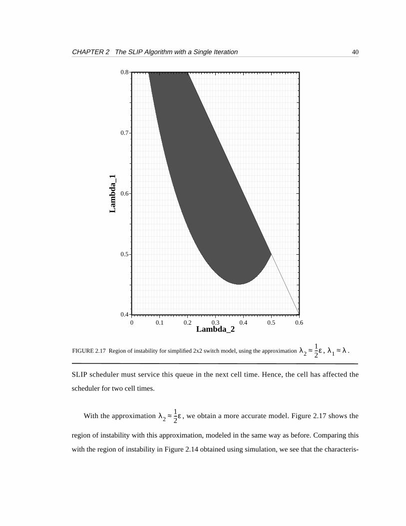
With the approximation , we obtain a more accurate model. Figure 2.17 shows the
region of instability with this approximation, modeled in the same way as before. Comparing this
with the region of instability in Figure 2.14 obtained using simulation, we see that the characteris-
λ212---ε≈
FIGURE 2.17 Region of instability for simplified 2x2 switch model, using the approximation , .λ212---ε≈ λ1 λ≈
0 0.1 0.2 0.3 0.4 0.5 0.60.4
0.5
0.6
0.7
0.8
Lambda_2
Lam
bda_
1
CHAPTER 2 The SLIP Algorithm with a Single Iteration 41
tics are very similar. The approximate model captures the non-monotonic behavior of SLIP close
to .
5.3.2 Drift Analysis of a 2x2 SLIP Switch: Second Approximation
In our first model we found that modeling the arrival process as unqueued i.i.d. Bernoulli
arrivals was inaccurate. This was because arriving cells in the real switch are queued and affect the
scheduler for multiple cell times. In this section we try and improve upon this approximation by
modeling the arrival process more accurately.
In our second approximation, we model arrivals as an on-off process, modulated by a 2-state
discrete-time Markov chain (DTMC). The DTMC is used to model thebusy andidle cycles of
input queues Q(1,2) and Q(2,1) in the real switch. When the DTMC is in thebusy state, cells are
arrive at rate 1, and when it is theidle state, cells arrive at rate 0. Using this model we attempt to
capture the correlation between successive cell times.
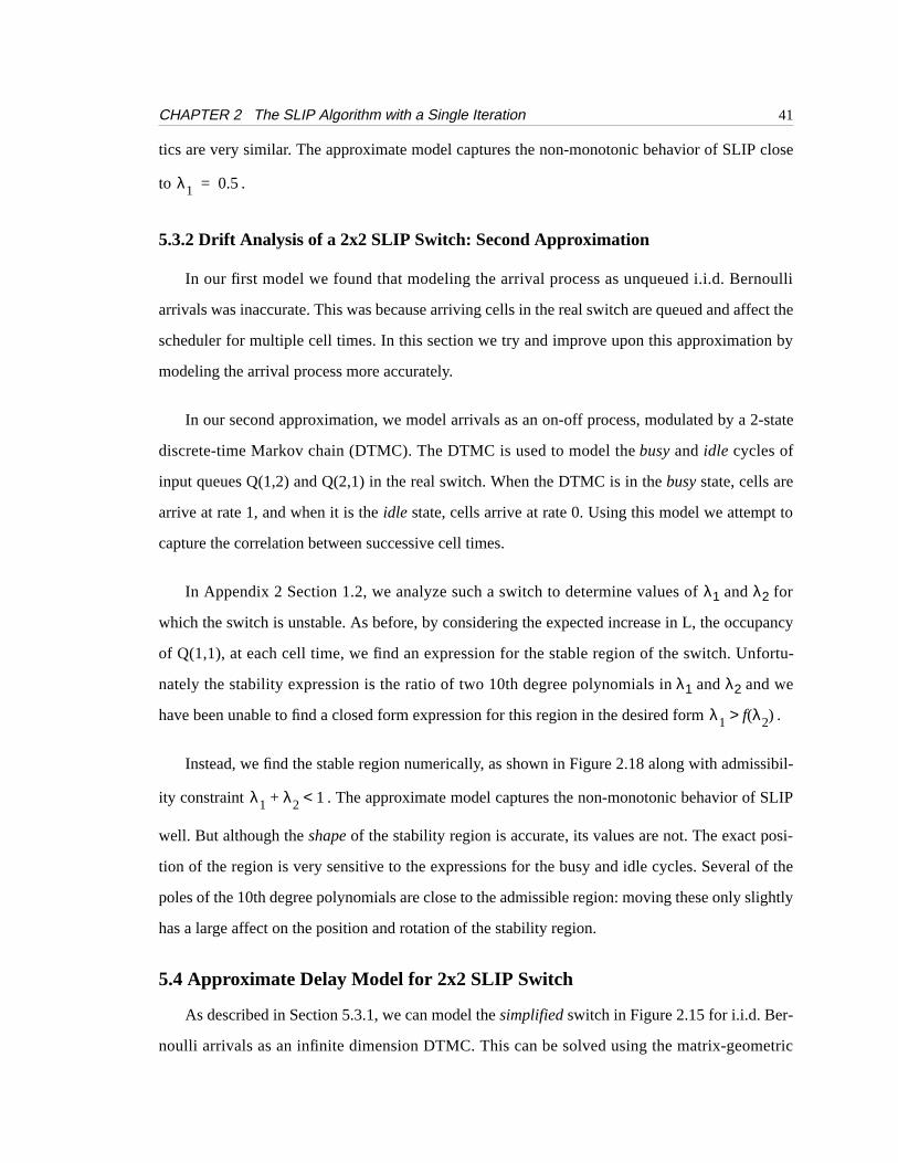
In Appendix 2 Section 1.2, we analyze such a switch to determine values ofλ1 and λ2 for
which the switch is unstable. As before, by considering the expected increase in L, the occupancy
of Q(1,1), at each cell time, we find an expression for the stable region of the switch. Unfortu-
nately the stability expression is the ratio of two 10th degree polynomials inλ1 and λ2 and we
have been unable to find a closed form expression for this region in the desired form .
Instead, we find the stable region numerically, as shown in Figure 2.18 along with admissibil-
ity constraint . The approximate model captures the non-monotonic behavior of SLIP
well. But although theshape of the stability region is accurate, its values are not. The exact posi-
tion of the region is very sensitive to the expressions for the busy and idle cycles. Several of the
poles of the 10th degree polynomials are close to the admissible region: moving these only slightly
has a large affect on the position and rotation of the stability region.
5.4 Approximate Delay Model for 2x2 SLIP Switch
As described in Section 5.3.1, we can model thesimplified switch in Figure 2.15 for i.i.d. Ber-
noulli arrivals as an infinite dimension DTMC. This can be solved using the matrix-geometric
λ1 0.5=
λ1 f λ2( )>
λ1 λ2 1<+
CHAPTER 2 The SLIP Algorithm with a Single Iteration 42
method of Neuts [36], and its solution is described in Appendix 2 Section 2. From the steady-state
distribution, (Appendix 2, Equation 20) we can evaluate the expected
occupancy of Q(1,1).
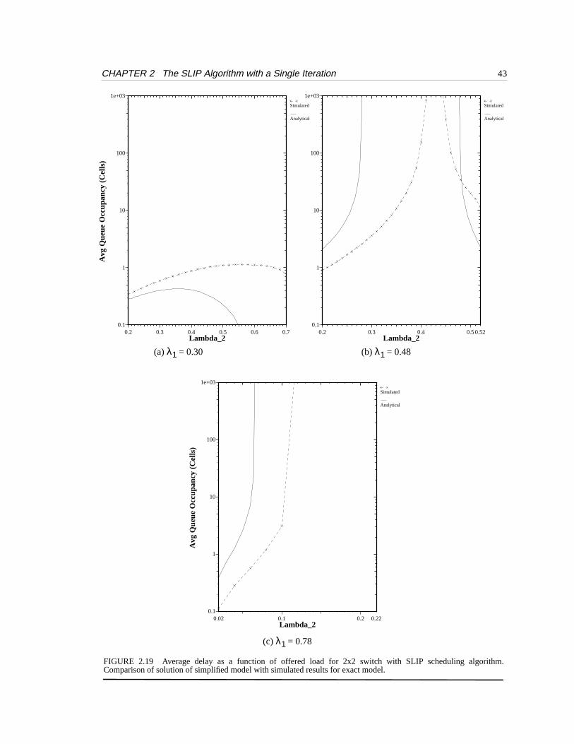
To determine how good our simplified model is, Figure 2.19 compares the expected delay of
thesimplified switch model to the simulated average delay of theactual switch with three queues
in Figure 2.12. We make the assumption introduced in Section 5.3.1 that . Graphs are
FIGURE 2.18 Region of stability for the approximate model of the switch in Figure 2.12 as a function ofλ1 andλ2.The admissibility constraintλ1 + λ2 < 1 is shown. The stable region lies between the two curves and below theadmissibility constraint.
0 0.1 0.2 0.3 0.4 0.5 0.6 0.7 0.80.4
0.5
0.6
0.7
0.8
0.9
1
Lambda_2
Lam
bda_
1
Π Π0 Π1 Π2 …, , ,[ ]=
ε 2λ2=
CHAPTER 2 The SLIP Algorithm with a Single Iteration 43
FIGURE 2.19 Average delay as a function of offered load for 2x2 switch with SLIP scheduling algorithm.Comparison of solution of simplified model with simulated results for exact model.
0.2 0.3 0.4 0.5 0.6 0.70.1
1
10
100
1e+03
Lambda_2
Avg
Que
ue O
ccup
ancy
(C
ells
) Simulated
Analytical
0.2 0.3 0.4 0.50.520.1
1
10
100
1e+03
Lambda_2
Simulated
Analytical
0.1 0.20.02 0.220.1
1
10
100
1e+03
Lambda_2
Avg
Que
ue O
ccup
ancy
(C
ells
)
Simulated
Analytical
(a)λ1 = 0.30 (b) λ1 = 0.48
(c) λ1 = 0.78

CHAPTER 2 The SLIP Algorithm with a Single Iteration 44
shown for representing respectively regions in which Q(1,1) is always
stable, non-monotonic and unstable.
As we found with the analytical solution for the stability region, the model of thesimplified
switch exhibits the same behavior as the actual switch, but the values for delay are quite different.
6 Variations on SLIP
6.1 Prioritized SLIP
Many applications use multiple classes of traffic with different priority levels. The basic SLIP
algorithm can be extended to include requests at multiple priority levels with only a small perfor-
mance and complexity penalty. We call this the Prioritized SLIP algorithm.
In Prioritized SLIP each input now maintains a separate FIFOfor each priority level and for
each output. This means that for an NxN switch with P priority levels, each input maintains PxN
FIFOs. We shall label the queue between inputi and outputj at priority levell, where
, . As before, only one cell can arrive in a cell time, so this does not require a
processing speedup by the input.
The Prioritized SLIP algorithm givesstrict priority to the highest priority request in each cell
time. This means that will only be served if all queues are empty.
The SLIP algorithm is modified as follows:
Step 1. Request. Input i selects the highest priority non-empty queue for outputj. Theinput sends the priority levellij of this queue to the outputj.
Step 2. Grant. If outputj receives any requests, it determines the highest level request. i.e.it finds . The output then chooses one input among only those inputsthat have requested at level . The output arbiter maintains a separate pointer, foreach priority level. When choosing among inputs at levelL(j), the arbiter uses the pointer
and chooses using the same round-robin scheme as before. The output notifieseach input whether or not its request was granted. The pointer is incremented(modulo N) to one location beyond the granted input if and only if inputi accepts outputjin step 3.
λ1 0.3 0.4 and 0.78,=
Ql i j,( )
1 i j, N≤ ≤ 1 l P≤ ≤
Ql i j,( ) Qm i j,( ) l m P≤<,
L j( ) maxi
l ij( )=L j( ) gjl
gjL j( )gjL j( )
CHAPTER 2 The SLIP Algorithm with a Single Iteration 45
Step 3. Accept. If input i receives any grants, it determines the highest level grant. i.e. itfinds . The input then chooses one output among only those that haverequested at level . The input arbiter maintains a separate pointer, foreach priority level. When choosing among outputs at level , the arbiter uses thepointer and chooses using the same round-robin scheme as before. The input noti-fies each output whether or not its grant was accepted. The pointer is incremented(modulo N) to one location beyond the accepted output.
Implementation of the Prioritized SLIP algorithm is more complex than the basic SLIP algo-
rithm, but can still be fabricated from the same number of arbiters. This is because each arbiter
only selects an input (output) among those requesting (granting) at the highest priority level. The
arbiter now consists of two parts: the first part determines the levell of the highest priority request
(grant) and removes those requests (grants) with levelsm<l; the second part of the arbiter is the
same round-robin arbiter as before. An implementation of Prioritized SLIP is described in Section
7.
6.2 Threshold SLIP
As we shall see in Chapter 4, scheduling algorithms that find a maximumweightmatch out-
perform those that find a maximumsized match. In particular, if the weight of the edge between
input i and outputj is the occupancyLi,j(t) of input queueQ(i,j) then we will conjecture that the
algorithm is stable for all admissible i.i.d. Bernoulli arrival patterns. But maximum weight
matches are significantly harder to calculate than maximum sized matches [41] and to be practical,
must be implemented using an upper limit on the number of bits used to represent the occupancy
of the input queue.
In the Threshold SLIP algorithm we make a compromise between the maximum sized match
and the maximum weight match by quantizing the queue occupancy according to a set of threshold
levels. The threshold level is then used to determine the priority level in the Priority SLIP algo-
rithm. Each input queue maintains an ordered set of threshold levels , where
. If then the input makes a request of level .
L' i( ) maxj
l ij( )=l ij L' i( )= ail
L' i( )aiL' i( )
aiL' i( )
T t1 t2 … tT, , ,{ }=
t1 t2 … tT< < < ta Q i j,( )≤ ta 1+< l i a=
CHAPTER 2 The SLIP Algorithm with a Single Iteration 46
6.3 Weighted SLIP
In some applications, the strict priority scheme of Prioritized SLIP may be undesirable, lead-
ing to starvation of low-priority traffic. The Weighted SLIP algorithm can be used to divide the
throughput to an output non-uniformly among competing inputs. The bandwidth from inputi to
outputj is now a ratio subject to the admissibility constraints .
In the basic SLIP algorithm each arbiter maintains an ordered circular list, .
In the Weighted SLIP algorithm the list is expanded at outputj to be the ordered circular list
where and inputi appears times
in .
6.4 Least Recently Used
When an output arbiter in SLIP successfully selects an input, that input becomes thelowest
priority in the next cell time. This is intuitively a good characteristic: the algorithm should least
favor connections that have been served recently. But which input should now have thehighest
priority? In SLIP, it is the next input that happens to be in the schedule. But this is not necessarily
the input that was servedleast recently. By contrast, the Least Recently Used (LRU) algorithm
gives highest priority to the least recently used and lowest priority to the most recently used.
LRU is identical to SLIP except for the ordering of the elements in the arbiter list: they are no
longer in ascending order of input number but rather are in an ordered list starting from the least
recently to most recently selected. If a grant is successful, the input that is selected is moved to the
end of the ordered list. Similarly, an LRU list can be kept at the inputs for choosing among com-
peting grants.
We might expect LRU to perform as well as, if not better than SLIP. But as we can see from
Figure 2.20, it performs significantly worse when the offered load is greater than 65%. This is
because the output arbiters do not tend todesynchronizeand several may grant to the same input,
as shown in Figure 2.21. Each schedule can become re-ordered at the end of each cell time which,
over many cell times, leads to a random ordering of the schedules. This in turn leads to a high
probability that the pointers at two or more outputs will point to the same input: the same problem
fijnij
dij------= fij
i∑ 1< fij
j∑ 1<,
S 1 … N, ,{ }=
Sj 1 … Wj, ,{ }= Wj LowestCommonMultipledij( )=nij
dij------ Wj×
Sj

CHAPTER 2 The SLIP Algorithm with a Single Iteration 47
encountered by RRM and PIM with a single iteration. This explains why the performance for PIM
and LRU are very similar.
FIGURE 2.20 LRU performs no better than PIM for a single iteration. Results shown for 16x16 switch with i.i.d.Bernoulli arrivals.
20 30 40 50 60 70 80 90 1000.1
1
10
100
1e+03
Offered Load (%)
Avg
Cel
l Lat
ency
(C
ells
)LRU
SLIP
PIM
FIFO

CHAPTER 2 The SLIP Algorithm with a Single Iteration 48
FIGURE 2.21 LRU performs poorly because of the synchronization between the output arbiters. Results shown for16x16 switch with i.i.d. Bernoulli arrivals.
0 10 20 30 40 50 60 70 80 90 1000
1
2
3
4
5
6
7
8
9
10
11
Offered Load (%)
Avg
Num
ber
of S
ynch
roni
zed
Out
put S
ched
uler
s
LRU
RRM
SLIP
CHAPTER 2 The SLIP Algorithm with a Single Iteration 49
7 Implementing SLIP
One of the objectives of this work was to design a scheduler that is simple to implement. To
conclude our description of SLIP, in this section we consider the complexity of implementing
SLIP in hardware, arguing that with current technology it is feasible to implement a centralized
scheduler for a 32x32 switch on a single chip.
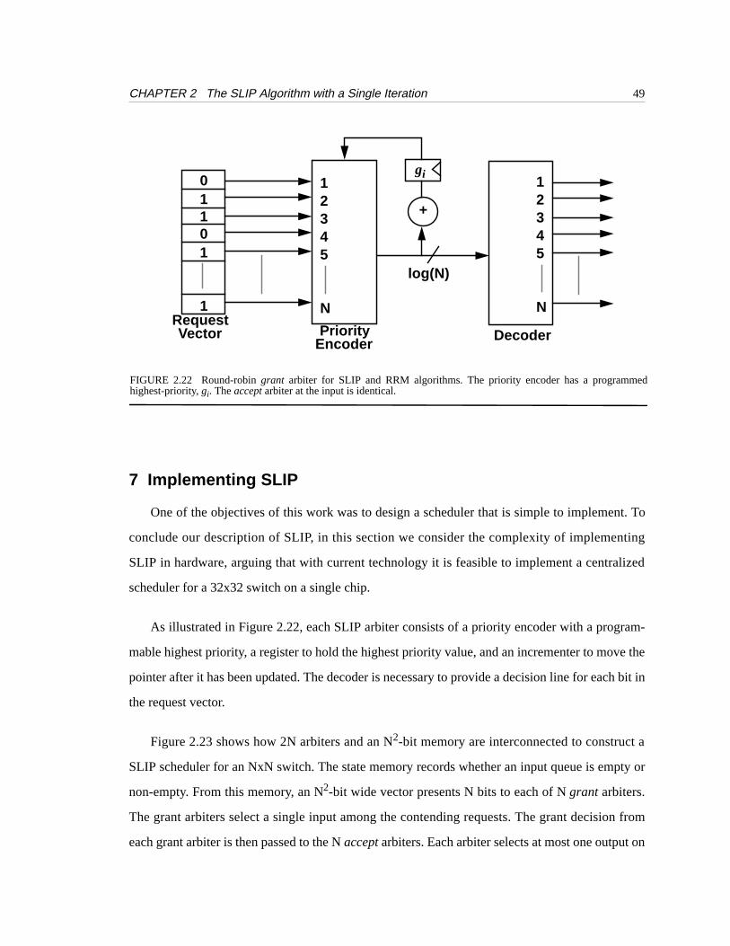
As illustrated in Figure 2.22, each SLIP arbiter consists of a priority encoder with a program-
mable highest priority, a register to hold the highest priority value, and an incrementer to move the
pointer after it has been updated. The decoder is necessary to provide a decision line for each bit in
the request vector.
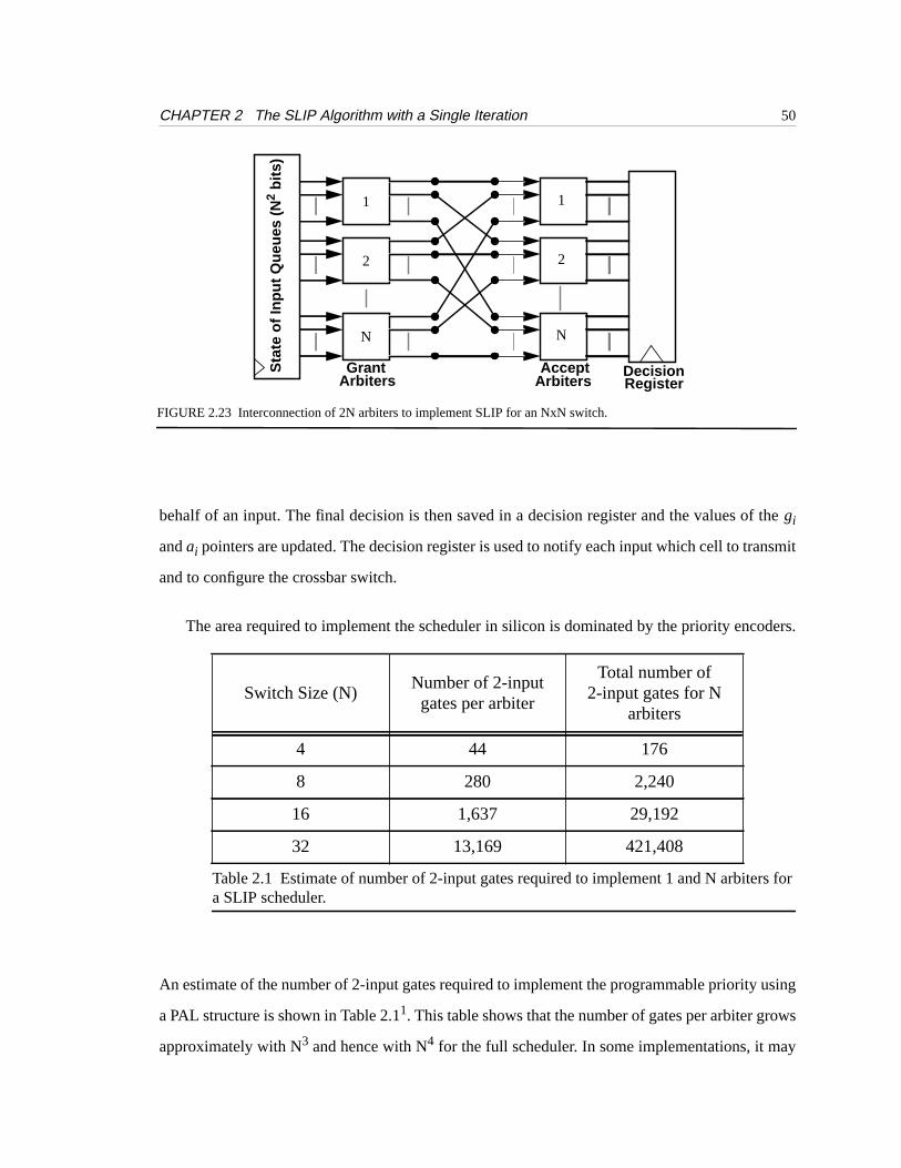
Figure 2.23 shows how 2N arbiters and an N2-bit memory are interconnected to construct a
SLIP scheduler for an NxN switch. The state memory records whether an input queue is empty or
non-empty. From this memory, an N2-bit wide vector presents N bits to each of Ngrant arbiters.
The grant arbiters select a single input among the contending requests. The grant decision from
each grant arbiter is then passed to the Naccept arbiters. Each arbiter selects at most one output on
12345
NRequestVector
+
gi
log(N)
01101
1
PriorityEncoder
FIGURE 2.22 Round-robingrant arbiter for SLIP and RRM algorithms. The priority encoder has a programmedhighest-priority,gi. Theaccept arbiter at the input is identical.
12345
N
Decoder
CHAPTER 2 The SLIP Algorithm with a Single Iteration 50
behalf of an input. The final decision is then saved in a decision register and the values of thegi
andai pointers are updated. The decision register is used to notify each input which cell to transmit
and to configure the crossbar switch.
The area required to implement the scheduler in silicon is dominated by the priority encoders.
An estimate of the number of 2-input gates required to implement the programmable priority using
a PAL structure is shown in Table 2.11. This table shows that the number of gates per arbiter grows
approximately with N3 and hence with N4 for the full scheduler. In some implementations, it may
Switch Size (N)Number of 2-inputgates per arbiter
Total number of2-input gates for N
arbiters
4 44 176
8 280 2,240
16 1,637 29,192
32 13,169 421,408
Table 2.1 Estimate of number of 2-input gates required to implement 1 and N arbiters fora SLIP scheduler.
GrantArbiters
AcceptArbiters
Sta
te o
f Inp
ut Q
ueue
s (N
2 bi
ts)
Decision
FIGURE 2.23 Interconnection of 2N arbiters to implement SLIP for an NxN switch.
1
2
N
1
2
N
Register
CHAPTER 2 The SLIP Algorithm with a Single Iteration 51
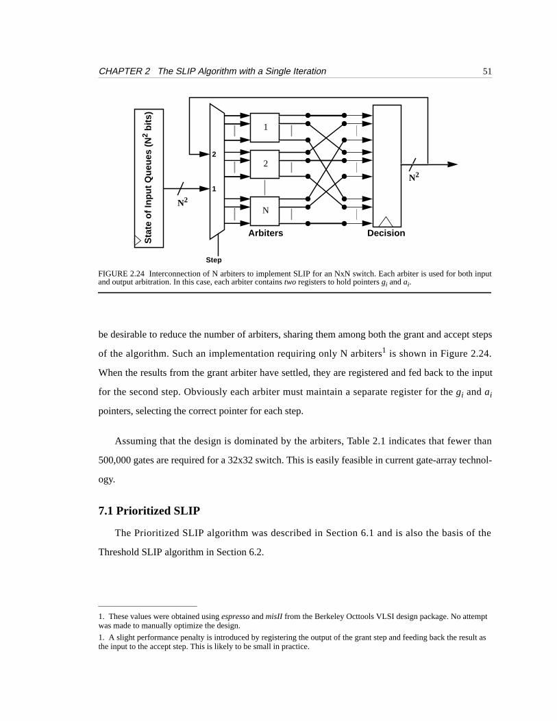
be desirable to reduce the number of arbiters, sharing them among both the grant and accept steps
of the algorithm. Such an implementation requiring only N arbiters1 is shown in Figure 2.24.
When the results from the grant arbiter have settled, they are registered and fed back to the input
for the second step. Obviously each arbiter must maintain a separate register for thegi andai
pointers, selecting the correct pointer for each step.
Assuming that the design is dominated by the arbiters, Table 2.1 indicates that fewer than
500,000 gates are required for a 32x32 switch. This is easily feasible in current gate-array technol-
ogy.
7.1 Prioritized SLIP
The Prioritized SLIP algorithm was described in Section 6.1 and is also the basis of the
Threshold SLIP algorithm in Section 6.2.
1. These values were obtained usingespresso andmisII from the Berkeley Octtools VLSI design package. No attemptwas made to manually optimize the design.
1. A slight performance penalty is introduced by registering the output of the grant step and feeding back the result asthe input to the accept step. This is likely to be small in practice.
Arbiters Decision
Sta
te o
f Inp
ut Q
ueue
s (N
2 bi
ts)
N2
N2
Step
2
1
FIGURE 2.24 Interconnection of N arbiters to implement SLIP for an NxN switch. Each arbiter is used for both inputand output arbitration. In this case, each arbiter containstwo registers to hold pointersgi andai.
1
2
N
CHAPTER 2 The SLIP Algorithm with a Single Iteration 52
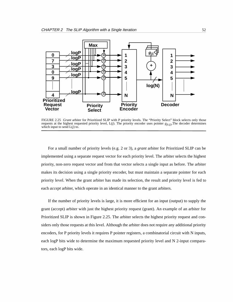
For a small number of priority levels (e.g. 2 or 3), agrant arbiter for Prioritized SLIP can be
implemented using a separate request vector for each priority level. The arbiter selects the highest
priority, non-zero request vector and from that vector selects a single input as before. The arbiter
makes its decision using a single priority encoder, but must maintain a separate pointer for each
priority level. When the grant arbiter has made its selection, the result and priority level is fed to
eachaccept arbiter, which operate in an identical manner to the grant arbiters.
If the number of priority levels is large, it is more efficient for an input (output) to supply the
grant (accept) arbiter with just the highest priority request (grant). An example of an arbiter for
Prioritized SLIP is shown in Figure 2.25. The arbiter selects the highest priority request and con-
siders only those requests at this level. Although the arbiter does not require any additional priority
encoders, for P priority levels it requires P pointer registers, a combinatorial circuit with N inputs,
each logP bits wide to determine the maximum requested priority level and N 2-input compara-
tors, each logP bits wide.
12345
NPrioritized
Vector
+
log(N)
07309
4
PriorityEncoder
12345
N
DecoderRequest
gj1=====
=
logPlogPlogPlogPlogP
logP
Max
PrioritySelect
FIGURE 2.25 Grant arbiter for Prioritized SLIP with P priority levels. The “Priority Select” block selects only thoserequests at the highest requested priority level, L(j). The priority encoder uses pointergjL(j).The decoder determineswhich input to send L(j) to.