the slow growth of new plants - umd
TRANSCRIPT

The Slow Growth of New Plants: Learning about Demand?
Lucia Foster
Bureau of the Census
John Haltiwanger
University of Maryland
and NBER
Chad Syverson
University of Chicago Booth
School of Business and NBER
January 2014
Abstract
It is well known that new businesses are typically much smaller than their established industry
competitors, and that this size gap closes slowly. We show that even in commodity-like product
markets, these patterns do not reflect productivity gaps, but rather differences in demand-side
fundamentals. We document and explore patterns in plants’ idiosyncratic demand levels by
estimating a dynamic model of plant expansion in the presence of a demand accumulation
process (e.g., building a customer base). We find active accumulation driven by plants’ past
production decisions quantitatively dominates passive demand accumulation, and that within-
firm spillovers affect demand levels but not growth. This demand accumulation process has
important implications for ongoing research in fields as diverse as industrial organization, macro,
finance, and trade.
We thank seminar participants at UC-Berkeley, UCLA, Carnegie Mellon, Colorado, Harvard, LSE, MIT, National
Bank of Belgium, Penn State, Princeton, SITE, the Cowles Conference, CAED, CEPR IO, and UBC Summer IO
meetings for their comments. We thank Lauren Deason for her excellent work developing the downstream demand
indicators. Contact information: Foster: Center for Economic Studies, Bureau of the Census, Washington, DC
20233; Haltiwanger: Department of Economics, University of Maryland, College Park, MD 20742; Syverson:
University of Chicago Booth School of Business, 5807 S. Woodlawn Ave., Chicago, IL 60637. Any opinions and
conclusions expressed herein are those of the authors and do not necessarily represent the views of the U.S. Census
Bureau. All results have been reviewed to ensure that no confidential information is disclosed.

2
1. Introduction
Researchers who have studied aspects of firm and industry dynamics have noted an
empirical regularity: new businesses—and for that matter, extensions of existing businesses built
in new markets—are smaller than established businesses in the same market, and this size gap
closes only slowly as the producer ages. (Dunne, Roberts, and Samuelson (1988), Caves (1998),
and Cabral and Mata (2003) offer some of the most systematic evidence, though this pattern has
been noted in individual markets in many studies.)
This pervasive pattern has colored explanations for businesses’ disparate outcomes in
fields as diverse as industrial organization, macro, finance, and trade. Recent theoretical efforts
in these fields have argued that demand dynamics are an explanation for this regularity. (See, for
example, Caminal and Vives (1999), Klepper (2002), Cabral and Mata (2003), Radner (2003),
Fishman and Rob (2003 and 2005), Bar-Isaac and Tadelis (2008), Arkolakis (2010), Dinlersoz
and Yorukoglu (2010), Gourio and Rudanko (2011), Luttmer (2011), Drozd and Nosal (2012),
and Perla (2013).) Specifically, new businesses are small because demand for their product is
low, and demand is low because of informational, reputational, or other frictions. Over time,
these frictions gradually subside, and demand for the business’s product grows—if it is robust
enough in the first place to prevent the business from exiting.
In this paper, we empirically explore this hypothesis using a sample of U.S.
manufacturing plants in commodity-like product industries (e.g., ready-mixed concrete,
cardboard boxes, manufactured ice). We first show that the size gaps between new and more
established plants are not the result of supply-side cost differences. New plants in our sample are
just as technically efficient as—and often even slightly more efficient than—older plants, and
have lower costs as a result. That is, entrants are small in spite of their costs, not because of
them.
After demonstrating that entrants’ small size and slow growth are not explained by cost
differences, we describe atheoretically how plants’ idiosyncratic demand fundamentals evolve in
the data. Then, to explain these patterns, we build and estimate a dynamic model of plant
expansion in the presence of a demand accumulation process (e.g., building a customer base,
though multiple interpretations of this process are possible). The model allows demand to
accumulate in two different ways. We term one “demand accumulation by being.” This is
exogenous growth in demand over time that the producer passively reaps as long as it survives to

3
operate in the future. The second is “demand accumulation by doing,” an endogenous
accumulation mechanism where the producer can actively influence its future demand by making
choices (namely, pricing) that build future demand stock at the expense of current profits. The
model, when taken to our data, allows us to qualitatively characterize these demand
accumulation processes and to measure the size of their relative influences.
The results indicate that our dynamic demand model can explain a considerable portion
of the relationship between plant age and average size. This is notable given that our data spans a
number of product markets and because those markets are for physically homogeneous,
commodity-like products, where one might think the role of demand variations is smaller than in
highly differentiated industries. We also find that the endogenous “demand accumulation by
doing” process plays a greater role in explaining the small size and slow growth of new plants
than does exogenous “demand accumulation by being,” though both channels have some
influence. Further, we are able to characterize some cross-sectional differences in demand levels
within similarly aged plants, showing for example that entering plants owned by firms that
already operate other plants elsewhere appear to enjoy some spillover demand capital benefits
from their corporate parent.
Besides informing the theoretical work on the role of dynamic demand discussed above,
this paper also fits into a new line of research that is extending the large empirical literature tying
productivity to plant and firm survival (see Bartelsman and Doms (2000) and Syverson (2011)
for surveys of this literature) by explicitly accounting for demand-side effects on plants’ growth
and survival. (Das, Roberts, and Tybout (2007); Eslava et al. (2008); Foster, Haltiwanger, and
Syverson (2008); Kee and Krishna (2008); and De Loecker (2011) are examples of the new
approach.) Earlier heterogeneous-productivity industry frameworks captured differences among
industry producers in a single index, often explicitly or implicitly taken to be producer
costs/productivity (e.g., Jovanovic (1982), Hopenhayn (1992), Melitz (2003), and Asplund and
Nocke (2006)). Related empirical work on business dynamics also did not make distinctions as
to the forms of heterogeneity (e.g., Dunne, Roberts, and Samuelson (1989a and 1989b); Troske
(1996); Pakes and Ericson (1998); Ábrahám and White (2006); Brown, Earle, and Telegdy
(2006)). The new research line expands the sources of heterogeneity to include both
technological and demand-based idiosyncratic profitability fundamentals, each following
separate (even independent) stochastic processes. The new framework therefore allows an
4
additional and realistic richness in the market forces that determine producers’ fates. Further,
this approach also suggests a reinterpretation of productivity’s effects as inferred from standard
measures. This is because typical productivity measures incorporate not just technology but also
demand-side effects through their (often unavoidable because of data limitations) inclusion of
producer prices in the output measure.
The paper proceeds as follows. The next section describes data and measurement issues.
Section 3 documents basic empirical facts about the evolution of producers’ idiosyncratic
demands in our sample. Section 4 describes the empirical model that we estimate using plants’
dynamic choices. The main empirical results are presented in Section 5. Section 6 discusses
alternative explanations and provides robustness checks and Section 7 concludes.
2. Data and Measurement Issues
This paper uses essentially the same data set of homogenous goods producers we used in
Foster, Haltiwanger, and Syverson (2008).1 Details on the selection of our sample and
construction of the variables we use are in the Appendix, so we only highlight key points here.
The data is an extract of the U.S. Census of Manufactures (CM). The CM covers the
universe of manufacturing plants and is conducted quinquenially in years ending in “2” and “7”.
We use the 1977, 1982, 1987, 1992, and 1997 CMs in our sample based upon the availability and
quality of physical output data. Information on plants’ production in physical units is important
because we must be able to observe plants’ output quantities and prices, not just total revenue
(often the only output measure available in producer microdata). The CM collects information
on plants’ shipments in dollar value and physical units by seven-digit SIC product category.2
1 We drop producers of one product that was included in the Foster, Haltiwanger, and Syverson (2008) sample:
gasoline. The current study requires not only contemporaneous data but lagged data starting in 1963 to construct
initial capital stocks and also lagged revenue measures. We found the historical data for the gasoline refining
industry was somewhat spotty, and this limited the number of industry plants for which we had valid data. We also
think that our learning about demand model is somewhat less well suited to gasoline products, especially since there
is so little entry in gasoline to identify our learning effects.
2 A problem with CMs prior to our sample is that it is more difficult to identify balancing product codes (these are
used to make sure the sum of the plant’s product-specific shipment values equals the plant’s separately reported total
value of shipments). Having reliable product codes is necessary to obtain accurate information on plants’ separate
quantities and prices, important inputs into our empirical work below. A related problem is that there are erratic
time series patterns in the number of establishments reporting physical quantities, especially in early CMs. We thus
choose to focus on the data in 1977 and beyond. However, we do use revenue data from prior censuses as far back
as 1963 when constructing plants’ ages and demand stocks.

5
The roughly 17,000 plant-year observations in the sample include producers of one of ten
products: corrugated and solid fiber boxes (which we will refer to as “boxes” from now on),
white pan bread (bread), carbon black, roasted coffee beans (coffee), ready-mixed concrete
(concrete), oak flooring (flooring), block ice, processed ice, hardwood plywood (plywood), and
raw cane sugar (sugar).3 These products were chosen because of their physical homogeneity
which allows plants’ output quantities and unit prices to be more meaningfully compared.
Note that physical homogeneity does not necessarily imply that producers operate in an
undifferentiated product market. Prices vary within industries because, for instance, geographic
demand variations or webs of history-laden relationships between particular consumers and
producers create producer-specific demand shifts. Further, quantities sold differ tremendously
even holding price fixed. Trying to explain why they differ is the very point of our analysis. Our
quantity data are meaningful not due to the complete absence of differentiation, but rather
because there is no differentiation along the dimension in which we measure output—the
physical unit. The notion behind the selection of our sample products is that a consumer should
be roughly indifferent between unlabeled physical units of the industry output. But that does not
have to imply that consumers view other products or services (real or perceived) tied to those
units of output as equivalent. Much of this sort of differentiation, we argue in our earlier work,
is horizontal rather than vertical in nature.
2.1. Idiosyncratic Demand: Concept and Measurement
Our descriptive characterization of plant-level idiosyncratic demand uses measures that
are obtained by estimating demand for each of the ten products in our sample. We borrow our
methodology from our earlier work in Foster, Haltiwanger, and Syverson (2008).
We begin by estimating the following demand function separately for each of our ten
3 Our product definitions are built up from the seven-digit SIC product classification system. Some of our ten
products are the only seven-digit product in their respective four-digit SIC industry, and thus the product defines the
industry. This is true of, for example, ready-mixed concrete. Others are single seven-digit products that are parts of
industries that make multiple products. Raw cane sugar, for instance, is one seven-digit product produced by the
four-digit sugar and confectionary products industry. Finally, some of our ten products are combinations of seven-
digit products within the same four-digit industry. For example, the product we call boxes is actually comprised of
roughly ten seven-digit products. In cases where we combine products, we base the decision on our impression of
the available physical quantity metric’s ability to capture output variations across the seven-digit products without
introducing serious measurement problems due to product differentiation. The exact definition of the ten products
can be found in the Appendix.
6
products:
(1) ln 𝑞𝑖𝑡 = 𝛼0 + 𝛼1 ln 𝑝𝑖𝑡 + ∑ 𝛼𝑡𝑌𝐸𝐴𝑅𝑡𝑡 + 𝛼2 ln(𝐼𝑁𝐶𝑂𝑀𝐸𝑚𝑡) + 𝜂𝑖𝑡,
where qit is the physical output of plant i in year t, pit is the plant’s price, and ηit is a plant-year
specific disturbance term. We also control for a set of demand shifters, including a set of year
dummies (YEARt), which adjust for any economy-wide variation in the demand for the product,
as well as the average income in the plant’s local market m (INCOMEmt). We define local
markets using the Bureau of Economic Analysis’ Economic Areas (EAs).4
Plant quantities are simply their reported output in physical units. We calculate unit
prices for each producer using the plant’s reported revenue and physical output.5 These prices
are then adjusted to a common 1987 basis using the revenue-weighted geometric mean of the
product price across all of the plants producing the product in our sample.
Of course, estimating the above equation using ordinary least squares (OLS) could lead to
positively biased estimates of the price elasticity α1. Producers may optimally respond to
positive (negative) demand shifts ηit by raising (reducing) prices, creating a positive correlation
between the error term and pit. A solution to this is to instrument for pit using supply-side (cost)
influences on prices. While such instruments can sometimes be hard to come by in practice, we
believe we have very suitable instruments at hand: namely, plants’ physical total factor
productivity (TFP) levels. Physical TFP is measured as the ratio of the plant’s output quantity in
physical units to its inputs, where the inputs are the standard composite index of labor, capital,
and intermediates weighted by their respective output elasticities. Physical TFP (which we
hereafter label TFPQ, where “Q” denotes quantity) embodies a producer’s technical efficiency—
its cost of producing a physical unit of output. As such, TFPQ levels should have explanatory
power over prices. They do; the correlation between plants’ logged TFPQ levels and their
logged prices in our sample is -0.54. Further, it is unlikely they will be correlated with any
short-run plant-specific demand shifts embodied in ηit. Hence they appear quite suitable as
instruments for plant prices.6
4 EAs are collections of counties usually, but not always, centered on Metropolitan Statistical Areas. The 172 EAs
are mutually exclusive and exhaustive of the land area of the United States. See U.S. Bureau of Economic Analysis
(1995) for detailed information.
5 The reported revenues and physical quantities are annual aggregates, so the unit price is an annual average. This is
equivalent to a quantity-weighted average of all transaction prices charged by the plant during the year.
6 There are two potential problems with using TFPQ as an instrument. The first is that selection on profitability can
lead to a correlation between TFPQ and demand at the plant level, even if the innovations to both series are

7
We report the price and income elasticity estimates from the above demand equation in
Appendix Table A.1. The results are reassuring about our estimation strategy. All estimated
price elasticities are negative, and for all but carbon black, they exceed one in absolute value.
This is what one should expect; price-setting producers should be operating in the elastic portion
of their demand curves. (Carbon black’s inelastic point estimate may be due to the small number
of producers of that product in our sample. We cannot in fact reject that carbon black producers
face elastic demand.) Further, all products, again except for carbon black, have more elastic IV
demand estimates than in the OLS estimations. This is consistent with the theorized simultaneity
bias present in the OLS results as well as the ability of TFPQ to instrument for endogenous
prices.
The idiosyncratic demand estimates for our sample plants are simply the residual from
this IV demand estimation, along with the estimated contribution of local income added back in.
Thus the measure essentially captures across-plant output variation that reflects shifts in the
demand curve rather than movements along the demand curve.
The dispersion of our producer-specific demand measure is huge. Its within-product-year
standard deviation is 1.16 (recall the measure’s units are logged output). This implies that a
plant sells 3.2 times as much output at a given price as another in its industry that is one standard
deviation lower in the idiosyncratic demand distribution. By way of comparison, the comparable
standard deviations of logged TFPQ and logged prices are 0.26 and 0.18, respectively.
3. Facts about Plants’ Idiosyncratic Demands
In this section, we empirically characterize some basic patterns in the evolution of plants’
idiosyncratic demand fundamentals. We undertake two related exercises. First, we compare how
our sample plants’ demand and supply fundamentals evolve with age. This comparison makes
clear that the small size and slow growth of new producers are not driven by supply side (cost)
orthogonal as assumed. Producers with a higher TFPQ draws can tolerate lower demand draws (and vice versa)
while still remaining profitable. The second potential problem is measurement error. We compute prices by
dividing reported revenue by quantity and any measurement error in physical quantities will overstate the negative
correlation between prices and TFPQ, potentially contaminating the first stage of the IV estimation. We describe in
Foster, Haltiwanger, and Syverson (2008) how we deal with these issues. We found the patterns of demand
estimates to be quite robust, reducing concerns about either measurement issue. In Tables 1-2 in the next section,
we use the innovation to TFPQ as the instrument since this approach is more consistent with the estimation approach
for demand and Euler equations used later in the paper. We also note that our focus on commodity-like products
mitigates possible concerns about potential correlations between product quality and TFPQ.

8
influences. Second, we explore how the relative levels and convergence of idiosyncratic demand
levels change with plants’ attributes—specifically, the type of firms to which plants are tied.
3.1. Average Size Trajectories Reflect Demand Differences, Not Supply Differences
The evolution in our sample of (logged) TFPQ and idiosyncratic demand across plants of various
ages is shown in Table 1. Plant-level demand can be thought of as the logged output a plant
would sell relative to the average plant in the industry, if all plants charged a common, fixed
price. We use four age categories. An “entrant” is a plant appearing for the first time in the
Census of Manufactures (CM).7 “Young” establishments are those that first appeared in the
census prior to the current time period; that is, they were entrants in the previous census.
Establishments first appearing two censuses back are “medium” aged, and establishments that
first appeared three or more censuses prior are classified as “old.” Thus, an entrant is less than 5
years old, a young plant is 5-9 years old, a medium plant is 10-14 years old, and an old plant is
15 years old or older. Plants that will exit (die) by the next CM are placed in their own category
(“exiter”). We separately regress plants’ TFPQ and demand levels on dummies for each age
category, with old plants as the excluded category. The specification also includes a full set of
industry-year fixed effects, so all comparisons are among plants in the same industry in a given
year.
The results in the table’s top row indicate that new plants have slightly higher TFPQ
levels than established (“old”) incumbents. By the time plants are over five years old, however,
this TFPQ advantage is indistinct from zero. Incidentally, we also find that exiters of any age are
less efficient than incumbents, consistent with the large literature on the subject.
The patterns are very different, however, for plants’ idiosyncratic demands ( shown in the
table’s bottom row). The coefficient on the entrant dummy implies that, at the same price, a new
plant will sell only 58 percent of the output of a plant in the same industry that is more than 15
years old of the output of a plant in the same industry that is more than 15 years old (the demand
measure’s units are logged output, so e-0.550 = 0.577). This gap is also slow to close. Young
plants would sell 67 percent of the output of an old plant, and even medium plants years old
would only sell 73 percent as much.
7 Because the CM includes all manufacturing plants in the U.S., we observe all entry and exit, though only at five-
year intervals.
9
Thus there is a clear dichotomy between the age profiles of plants’ physical productivity
and demand-side fundamentals. Plants’ average technical efficiency levels are basically
invariant to age. What little difference that does exist—new entrants are slightly more efficient
and thus have slightly lower costs—would tend to make new plants larger than incumbents, the
opposite of the patterns seen in the data. On the other hand, there are clear age-related patterns
in plants’ average idiosyncratic demands. New plants have much lower demand than incumbents
in their industries. Moreover, these demand gaps close very slowly over time. Such patterns are
consistent with the growth trajectories observed in the data.
3.2. Cross-Sectional Differences in Demand Levels and Trajectories
Now consider the following example designed to illustrate how idiosyncratic demand
may change with plants’ characteristics. Two new plants are built in an industry: one plant is a
de novo entry by a firm with no prior experience; the other plant is opened by a large firm that
operates other plants as well, perhaps but not necessarily in the same industry and geographic
area. We might expect that the latter will enter with a higher level of demand. Customers may
already be familiar with the plant’s product, or at least its firm. This familiarity might also
impact the speed at which demand convergence occurs.
To explore these possibilities, we again project plants’ idiosyncratic demand measures on
plant age indicators but this time interact those indicators with a dummy for plants that are part
of a multi-plant firm. The firm’s other plants need not make the same product, or even be
manufacturers for that matter. This is essentially a crude proxy for firm size. Such multi-plant
firms account for 59 percent of the observations in our sample.
The results looking at the impact of multi-plant firm status are shown in Table 2. The
upper row shows the coefficients on the age categories, the lower those for the age categories
interacted with the multi-plant firm indicator. Hence the upper row shows the evolution of
idiosyncratic demand for single-unit plant/firms, while the column-wise sum of the two rows’
values reflects the same evolution for plants in multi-plant firms. Note that the excluded group is
different here from that in Table 1. The excluded group in Table 1 is all old plants-here, it is
only old plants in single-unit firms. Hence the age coefficients in the table show average
idiosyncratic demands relative to this group rather than all old plants. Since, as we will see, old
10
plants in multi-plant firms are the largest plants in our sample, their separation from the excluded
group is noticeable.
Single-unit plants exhibit similar patterns to those seen before for the whole sample.
Entrants have considerably smaller idiosyncratic demand levels than do established incumbents;
they sell 27 percent less output at a given price than do old single-unit plants, and they undersell
old multi-unit plants by 58 percent. There is some convergence between entry and being young ,
where young single-unit plants have demand levels 16 percent below old single-unit plants.
Convergence then largely stalls; medium-aged single-unit plants still have 14 percent demand
deficits.
For plants in multi-plant firms, similar qualitative relationships are present, but their
demand levels are significantly higher than single-unit plants at every age. That said, they are
still considerably smaller than old plants in multi-unit firms, with average demand levels for new
plants that are only two-thirds that of their older counterparts. Convergence is also slow among
multi-unit plants. Interestingly, exiting plants in multi-unit firms have lower average demand
levels than single-unit exiters.
It therefore appears that new plants in small firms (by our crude size measure) face
significantly lower idiosyncratic demand levels than do their new competitors in multi-plant
firms. Nevertheless, both types of plants see the inertial convergence patterns observed in the
broader sample, suggesting demand dynamics are at work in both cases.8 We develop a model of
dynamic, endogenous demand accumulation in the next section that we will take to our sample to
further investigate the nature of the accumulation process.
4. Model
The previous section’s analyses show that demand-side dynamics drive the relationship
between average plant size and age, and that plants’ idiosyncratic demands are related to the
attributes of the plants and the firms that own them. The patterns suggest dynamic demand
8 Of course, single-unit plants are not restricted to remaining in single-unit firms their entire life, nor for that matter
are multi-unit plants restricted to that type of firm. The more common transformation between these is for a plant in
a single-unit firm to become part of a multi-unit firm, either through acquisition by another firm or through its own
firm acquiring additional plants. From this perspective, the low demand levels and slow convergence of single-unit
entrants becomes even starker vis-à-vis their demand levels relative to old plants in multi-unit firms. In the
appendix we also show that the patterns in Tables 1 and 2 are robust to controlling for firm age (see Table A.2).
That is, there is slow growth of new plants even in large, mature firms.

11
factors are at play. Our proposed explanation involves dynamic demand side forces, growth of a
customer base or building a reputation (for example), that take considerable time to play out.
These forces lead to gradual growth of an entrant’s “demand stock,” at least among entrants good
enough to survive. The uncertainties tied to such processes may also create for the business an
option value of waiting to expand until further information about demand is revealed (e.g., Dixit
and Pindyck (1994)). It is also likely that the rate of demand stock growth and the level of
uncertainty are related to the characteristics of a plant or the firm that owns it.
We purposefully only loosely microfound the processes behind demand stock growth in
our model, as demand growth likely has multiple sources among the industries in our sample and
across producers more broadly. These could include customer learning through “word of
mouth,” the firm’s own advertising efforts, the blossoming of producer-customer relationships
through repeated interactions, or several other possibilities. It can involve expansion of
downstream buyers on either the extensive or intensive margin. We refer to the process
generically as “learning,” but the building of any sort of relationship capital along buyer-supplier
links fits our conceptual framework.9 What we seek to do here is characterize the basic
mechanics of that generic process and investigate how it interacts with producer behavior.
We assume the plant faces an isoelastic contemporaneous demand curve:
(2) 𝑞𝑡 = 𝜃𝑡𝐴𝑔𝑒𝑡𝜙
𝑍𝑡𝛾
𝑝𝑡−𝜂
,
where pt is the current price charged by the plant. Several factors shift the demand curve. t is
an exogenous demand shock that we assume follows an AR(1) process. Aget is the plant’s age.
Along with parameter , this accounts for deterministic changes in plants’ demand as they age.
Finally, Zt is a demand shifter that with parameter links a plant’s current activity to its future
expected demand level. Specifically, we assume Zt evolves according to the following process:
(3) 𝑍𝑡 = (1 − 𝛿)𝑍𝑡−1 + (1 − 𝛿)𝑅𝑡−1.
Thus, Zt is a sort of operating history of the plant. It grows with past plant sales Rt-1
subject to depreciation at a rate δ. Sales are measured as pt-1qt-1 (where qt is the plant’s current
9 Our read of the evidence is that the customer “learning” that drives demand stock growth is much broader than the
simple process of buyers finding out about the existence of a producer. While spotty information about mere
existence might be consistent with the large gaps in idiosyncratic demand present at plants’ births, it seems unlikely
to explain why convergence takes upwards of 15 years. We posit that learning involves much deeper components,
like details of producers’ product attributes, the quality and quantity of their bundled services, the consistency of
their operations, their expected longevity, and so on. Having to learn about these features can impart considerable
inertia into producers’ demand stocks.

12
output; we use lagged rather than current sales only for analytical convenience), This process
captures dynamic demand processes where a plant’s potential customer base is related to its past
sales activity. For instance, the process embodies many types of “word of mouth” effects
consumers are more likely to have heard about a producer or its product if it has operated more
in the past. This nests the demand-side analog to the specification common in the supply-side
learning-by-doing literature, where learning depends only on cumulative output; i.e., δ = 0. We
consider both this and the more general specification in our estimation.
On the supply side, the plant’s production function is given by
(4) 𝑞𝑡 = 𝐴𝑡𝑥𝑡,
where At is its TFPQ level, and xt is its input choice. This input can be thought of as a composite
of labor, capital, energy, and materials inputs, weighted appropriately. (For example, if the
technology is Cobb-Douglas and there are constant returns to scale, the composite would be the
plant’s inputs raised to their respective input elasticities.) The plant faces two costs: a factor cost
of wt per unit of xt and a fixed operating cost of f per period. The factor cost, given the form of
the production function and the role of TFPQ in it, implies the plant’s (constant) marginal cost is
ct = wt/At.
Using (2) to write a plant’s revenues in terms of its quantity gives an expression for the
plant’s periodic profit function:
(5) 𝜋𝑡 = 𝜃𝑡
1
𝜂𝐴𝑔𝑒𝑡
𝜙
𝜂 𝑍𝑡
𝛾
𝜂𝑞𝑡
1−1
𝜂 − 𝑐𝑡𝑞𝑡 − 𝑓 = 𝑅𝑡(𝑍𝑡, 𝑞𝑡) − 𝑐𝑡𝑞𝑡 − 𝑓.
The plant manager maximizes the present value of the plant’s operating profits.10 This
problem can be expressed recursively as follows:
(6) 𝑉(𝑍𝑡, 𝐴𝑡, 𝐴𝑔𝑒𝑡 , 𝜃𝑡) = max𝜒𝑡
{0(1 − 𝜒𝑡), 𝜒𝑡 supqt𝑅𝑡(𝑍𝑡, 𝑞𝑡) − 𝑐𝑡𝑞𝑡 − 𝑓 +
𝛽𝐸𝑉(𝑍𝑡+1, 𝐴𝑡+1, 𝐴𝑔𝑒𝑡+1, 𝜃𝑡+1)},
where V() is the plant’s value given state variables, and χt is the plant’s continuation decision (χt
= 1 if the plant continues to operate, while χt = 0 if the plant shuts down). Zt is endogenously
affected by the plant’s input choices; the plant’s age, TFPQ At, and demand shock t evolve
exogenously. The plant discounts the future by a factor of < 1.
10 We abstract from any agency issues that may arise between plants’ managers and the owners of these
establishments (if they are different people).

13
The plant’s continuation decision is made explicit in (6). It can operate (χt = 1) and earn
the profits this entails, or it can exit (χt = 0) and earn the outside option, normalized to zero here.
If it chooses to operate, it takes as given its past operating history as summarized in Zt and
chooses current production qt to maximize its present value. This choice of qt simultaneously
pins down the plant’s price and revenues through the demand curve.
The dynamics inherent in the plant’s choice problem are apparent: by producing more
(equivalently: pricing lower) today, the plant can shift out its demand curve tomorrow. The
optimal production level (price) in this case will be higher (lower) than that implied by a purely
static problem where current price is not tied to future demand. This is consistent with what we
found in Foster, Haltiwanger, and Syverson (2008): young plants in our sample had lower
average prices than older plants in the same industry.
It is important to note that the only source of dynamics in this model comes through the
demand process. If other dynamic forces affect plant behavior, they will be interpreted through
the lens of our model as demand. It is therefore important that we consider any other such forces
and how they might impact the interpretation of our results. We do this in detail in Section 6.
Optimal dynamic behavior (the plant’s qt trajectory) is given by the Euler equation
(derivation in the appendix):
(7) 𝑐𝑡
𝑝𝑡− (1 −
1
𝜂) = 𝛽(1 − 𝛿)𝐸 {𝜒𝑡+1 [
𝑐𝑡+1
𝑝𝑡+1− (1 −
1
𝜂) +
𝛾
𝜂
𝑐𝑡+1
𝑝𝑡+1
𝑅𝑡+1
𝑍𝑡+1]},
where again 𝜒𝑡+1 = 1 if the plant survives.11 Note that in deriving this expression, we have used
the demand curve to substitute out for the unobservable state variable 𝜃𝑡, which makes
estimation of the Euler equation much simpler.
The intuition behind the plant’s optimal dynamic behavior can be seen in this Euler
equation. The first term on the left hand side is the inverse of the plant’s price-to-marginal-cost
ratio. The second term is a function of the elasticity of demand familiar as the inverse of the
optimal markup for a firm facing a residual demand elasticity of –. Thus in a completely static
production/pricing optimization problem, the left hand side of the equation would be zero. It is
not generally so here because of the dynamics discussed above. Because the plant shifts out its
demand curve tomorrow by selling more today, it will markup price less over marginal cost than
11 This representation of the Euler equation with the possibility of exit is consistent with Pakes (1994) and
Aguirregabiria (1997). In the estimation process we discuss below, we build on the approaches of Aguirregabiria
(1997) and Alonso-Borrego (1998) for addressing this selection issue.

14
in a static world to induce extra sales. Another way to think about this is that now its marginal
revenue is not just what is implied by the contemporaneous demand function. It also includes
the effect on the discounted expected increase in future demand via growth of “demand stock” Z.
With a lower markup than implied by the static rule, the cost-price ratio in the first term will be
larger than the second term, and the left hand side will therefore generally be positive.
The first two terms in the square brackets on the right hand side are the same markup
function as that on the left hand side of the Euler equation, except for the next period. Of course,
being in the future, this is affected by discounting and the depreciation of Zt, and it holds in
expectation rather than ex-post. Again, this term would be zero in a static setting but is generally
positive here due to demand dynamics.
The third right-hand-side term in the square brackets depends on the ratio of the plant’s
expected next-period revenue to its operating history as captured in Zt+1. (Note that Zt+1 is known
at the end of period t, as it is solely a function of period-t values; see (3).) This term is positive
as long as the endogenous impact of past sales on demand is positive (i.e., as long as is
positive).
The Euler equation governs the rate at which the plant’s cost-price ratio falls, or
equivalently, how quickly it raises its price-cost markup. If = 0, future demand does not depend
on current production, and the solution to the Euler equation is for the plant to charge the optimal
static markup. If on the other hand > 0, the plant will charge a markup below the static
monopoly level. Notice that for plants that have been operating a long time, the ratio of (flow)
revenues to demand stock Rt+1/Zt+1 will tend to be small. Thus for these plants, the third term on
the right hand side will be small and the solution to the Euler equation will imply a price-cost
markup close to the static optimum. Therefore in general the demand dynamics imply that a new
plant starts out with a markup that may be considerably lower than the static optimum given the
price sensitivity it faces, and it then gradually raises its markup toward the static solution as its
demand stock grows large relative to its current revenues.
The Euler equation (7) can be further simplified by noting that Rt = ptqt, defining total
variable costs as Ct = ctqt (recall that the production function has constant returns), and
multiplying both the numerator and the denominator of the cost-price ratio by the plant’s
quantity as needed. This yields
(7a) 𝐶𝑡
𝑅𝑡− (1 −
1
𝜂) = 𝛽(1 − 𝛿)𝐸 {𝜒𝑡+1 [
𝐶𝑡+1
𝑅𝑡+1− (1 −
1
𝜂) +
𝛾
𝜂
𝐶𝑡+1
𝑍𝑡+1]}.
15
Both plants’ variable costs and revenues are readily observable in our data, and Zt is constructed
from past revenues. Thus we can observe all of the components of the Euler equation up to
parameters.
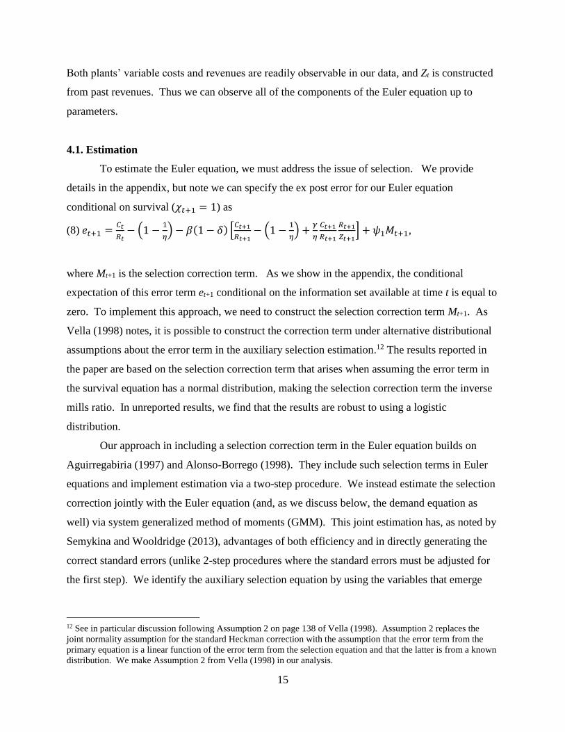
4.1. Estimation
To estimate the Euler equation, we must address the issue of selection. We provide
details in the appendix, but note we can specify the ex post error for our Euler equation
conditional on survival (𝜒𝑡+1 = 1) as
(8) 𝑒𝑡+1 =𝐶𝑡
𝑅𝑡− (1 −
1
𝜂) − 𝛽(1 − 𝛿) [
𝐶𝑡+1
𝑅𝑡+1− (1 −
1
𝜂) +
𝛾
𝜂
𝐶𝑡+1
𝑅𝑡+1
𝑅𝑡+1
𝑍𝑡+1] + 𝜓1𝑀𝑡+1,
where Mt+1 is the selection correction term. As we show in the appendix, the conditional
expectation of this error term et+1 conditional on the information set available at time t is equal to
zero. To implement this approach, we need to construct the selection correction term Mt+1. As
Vella (1998) notes, it is possible to construct the correction term under alternative distributional
assumptions about the error term in the auxiliary selection estimation.12 The results reported in
the paper are based on the selection correction term that arises when assuming the error term in
the survival equation has a normal distribution, making the selection correction term the inverse
mills ratio. In unreported results, we find that the results are robust to using a logistic
distribution.
Our approach in including a selection correction term in the Euler equation builds on
Aguirregabiria (1997) and Alonso-Borrego (1998). They include such selection terms in Euler
equations and implement estimation via a two-step procedure. We instead estimate the selection
correction jointly with the Euler equation (and, as we discuss below, the demand equation as
well) via system generalized method of moments (GMM). This joint estimation has, as noted by
Semykina and Wooldridge (2013), advantages of both efficiency and in directly generating the
correct standard errors (unlike 2-step procedures where the standard errors must be adjusted for
the first step). We identify the auxiliary selection equation by using the variables that emerge
12 See in particular discussion following Assumption 2 on page 138 of Vella (1998). Assumption 2 replaces the
joint normality assumption for the standard Heckman correction with the assumption that the error term from the
primary equation is a linear function of the error term from the selection equation and that the latter is from a known
distribution. We make Assumption 2 from Vella (1998) in our analysis.
16
from the selection model and analysis in Foster, Haltiwanger and Syverson (2008). Specifically,
plant-level physical productivity, prices, and capital stock are used in the selection equation.
Capital stock is not used as an instrument in the Euler or demand equations, so the selection
correction is identified in part on this basis.
In estimating the Euler equation by using GMM we take advantage of the property that
the ex post error is orthogonal to variables dated t and earlier. These include lagged cost-revenue
ratios, lagged revenues, and age dummies.
We include the demand equation (2) as part of our system GMM estimation for two
reasons. First, estimating the demand equation along with the Euler equation lets us recover the
impact of age. Notice that the effect of age on plant demand () is missing from the Euler
equation (7a) because substituting out for the unobservable θt using the demand curve causes the
Aget terms to cancel. Second, joint estimation also imposes additional structure that lets us
harness additional data variation to identify the model’s parameters.
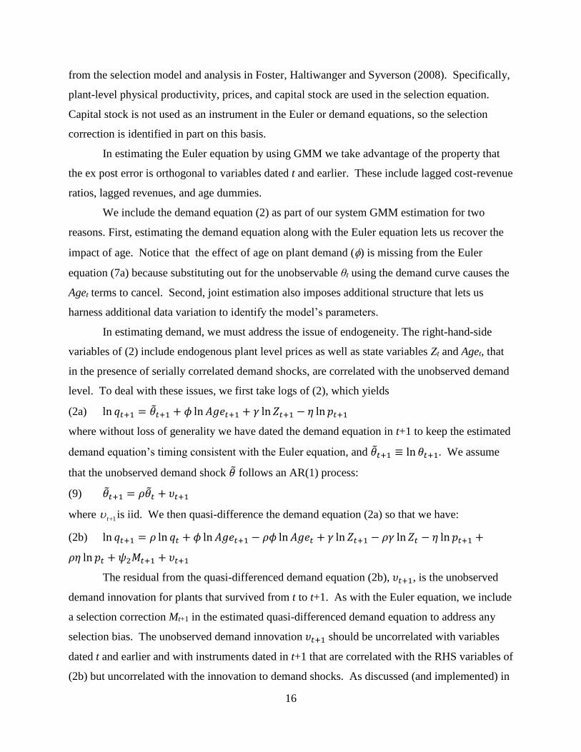
In estimating demand, we must address the issue of endogeneity. The right-hand-side
variables of (2) include endogenous plant level prices as well as state variables Zt and Aget, that
in the presence of serially correlated demand shocks, are correlated with the unobserved demand
level. To deal with these issues, we first take logs of (2), which yields
(2a) ln 𝑞𝑡+1 = �̃�𝑡+1 + 𝜙 ln 𝐴𝑔𝑒𝑡+1 + 𝛾 ln 𝑍𝑡+1 − 𝜂 ln 𝑝𝑡+1
where without loss of generality we have dated the demand equation in t+1 to keep the estimated
demand equation’s timing consistent with the Euler equation, and �̃�𝑡+1 ≡ ln 𝜃𝑡+1. We assume
that the unobserved demand shock �̃� follows an AR(1) process:
(9) �̃�𝑡+1 = 𝜌�̃�𝑡 + 𝜐𝑡+1
where 1t is iid. We then quasi-difference the demand equation (2a) so that we have:
(2b) ln 𝑞𝑡+1 = 𝜌 ln 𝑞𝑡 + 𝜙 ln 𝐴𝑔𝑒𝑡+1 − 𝜌𝜙 ln 𝐴𝑔𝑒𝑡 + 𝛾 ln 𝑍𝑡+1 − 𝜌𝛾 ln 𝑍𝑡 − 𝜂 ln 𝑝𝑡+1 +
𝜌𝜂 ln 𝑝𝑡 + 𝜓2𝑀𝑡+1 + 𝜐𝑡+1
The residual from the quasi-differenced demand equation (2b), 𝜐𝑡+1, is the unobserved
demand innovation for plants that survived from t to t+1. As with the Euler equation, we include
a selection correction Mt+1 in the estimated quasi-differenced demand equation to address any
selection bias. The unobserved demand innovation 𝜐𝑡+1 should be uncorrelated with variables
dated t and earlier and with instruments dated in t+1 that are correlated with the RHS variables of
(2b) but uncorrelated with the innovation to demand shocks. As discussed (and implemented) in

17
section 2.1, TFPQ is a valid instrument for plant-level prices in the demand equation. We use
this instrument here as well.
Estimation of this demand equation relies on variation (both across plants and within
plants over time) in age, past revenues, and cost-driven price shifts for identification. A
challenge in the estimation of (2b) is to obtain sufficient variation in the data to identify
separately the dynamics of the unobserved demand shock, the role of plant age and the role of
learning about demand through experience. It is partly due to these identification challenges that
we also exploit the variation important for identification of the Euler equation, (7a).
A basic measurement and estimation issue for both the demand and Euler equations is to
construct measures of the demand stock, Z. We observe plant revenues in every Census of
Manufactures back to 1963, so Rt is directly observable. Past revenues can be used to construct
the plant’s demand stock Zt as a function of past sales and the depreciation rate:
(3a) 𝑍𝑡 = (1 − 𝛿)𝜏𝑍𝑡−𝜏 + ∑ (1 − 𝛿)𝑖𝑍𝑡−𝑖𝜏𝑖=1 ,
where is the number of periods the plant has operated.
The remaining issue for measuring demand stocks is how to initialize Z for entrants, Z0.
Here, we draw insights from the descriptive empirical results in Section 3. We allow a plant’s
initial demand stock to be a function of the structure of the firm that owns it. Specifically, we
specify the initial demand stock of plant e as
(10) 𝑍0𝑒 = (𝐾0𝑒)𝜆1 (𝐾0𝑠(𝑒)+𝐾0𝑒
𝐾0𝑒)
𝜆2
,
where K0e is the initial physical capital stock of e, K0s(e) is the sum of the physical capital stocks
of plant e’s siblings (i.e., the total capital stock that year of the other plants owned by the same
firm within manufacturing), and 1 and 2 are parameters. The logic behind (10) is that a plant’s
initial demand stock can be related to its own physical size (K0e) as well as the size of its owning
firm. This specification therefore incorporates the possibility, seen in the previous section’s
results, that entrants of larger firms start with larger idiosyncratic demand levels than do those of
smaller firms. Note that (10) mechanically allows for single-plant firm entrants, where the
entrant is the firm, because in that case K0s(e) = 0 and the ratio in the parentheses is unity.
Additionally, (10) nests the possibility that multi-plant firm entrants do not have initial demand
advantages, which would be the case if 2 = 0. This specification lets the data tell us how
18
important the owning firm’s characteristics are in determining the initial demand stock of a new
plant.13
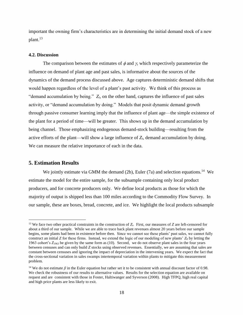
4.2. Discussion
The comparison between the estimates of and , which respectively parameterize the
influence on demand of plant age and past sales, is informative about the sources of the
dynamics of the demand process discussed above. Age captures deterministic demand shifts that
would happen regardless of the level of a plant’s past activity. We think of this process as
“demand accumulation by being.” Zt, on the other hand, captures the influence of past sales
activity, or “demand accumulation by doing.” Models that posit dynamic demand growth
through passive consumer learning imply that the influence of plant age—the simple existence of
the plant for a period of time—will be greater. This shows up in the demand accumulation by
being channel. Those emphasizing endogenous demand-stock building—resulting from the
active efforts of the plant—will show a large influence of Zt, demand accumulation by doing.
We can measure the relative importance of each in the data.
5. Estimation Results
We jointly estimate via GMM the demand (2b), Euler (7a) and selection equations.14 We
estimate the model for the entire sample, for the subsample containing only local product
producers, and for concrete producers only. We define local products as those for which the
majority of output is shipped less than 100 miles according to the Commodity Flow Survey. In
our sample, these are boxes, bread, concrete, and ice. We highlight the local products subsample
13 We face two other practical constraints in the construction of Zt. First, our measures of Z are left-censored for
about a third of our sample. While we are able to trace back plant revenues almost 20 years before our sample
begins, some plants had been in existence before then. Since we cannot see these plants’ past sales, we cannot fully
construct an initial Z for these firms. Instead, we extend the logic of our modeling of new plants’ Z0 by letting the
1963 cohort’s Z1963 be given by the same form as (10). Second, we do not observe plant sales in the four years
between censuses and can only build Z stocks using observed revenues. Essentially, we are assuming that sales are
constant between censuses and ignoring the impact of depreciation in the intervening years. We expect the fact that
the cross-sectional variation in sales swamps intertemporal variation within plants to mitigate this measurement
problem.
14 We do not estimate β in the Euler equation but rather set it to be consistent with annual discount factor of 0.98.
We check the robustness of our results to alternative values. Results for the selection equation are available on
request and are consistent with those in Foster, Haltiwanger and Syverson (2008). High TFPQ, high real capital
and high price plants are less likely to exit.

19
since it is possible that our model is better suited to such products, or it could be that the
parameters of demand accumulation dynamics might easily be different for these products. The
concrete-only subsample enables us to focus on a specific product where we have many
observations, permitting estimation of industry-specific parameters. We would prefer to let all
parameters vary across all products in our estimation, but some of our 10 sample industries
simply do not have enough plant-year observations to separately identify their industry’s
parameters with any useful precision. These subsamples serve as an alternative means of
exploring the robustness of our findings across products. However, we do also report some
results below where we permit key parameters to vary as a function of the industry’s attributes.
The variables included in our estimated model are defined as above, however, we make
one change in the demand specification from (2b). Rather than imposing the constant-elasticity
form shown in the equation, we allow the influence of plant age to vary non-parametrically. We
include a set of plant age dummies in the estimated version of (2b): a young dummy equal to one
if the plant in period t is one census period (i.e., 5-9 years) old, and a medium age dummy equal
to one if the plant is two census periods (10-14 years) old. The omitted group consists of mature
plants at least three census periods (15+ years) old in period t. (We have no entrants in the
estimation sample because we need to use lagged variables to identify the dynamic parameters.)
We also include controls in the demand equation not explicitly referenced in the above
discussion of the model. Because we are pooling data across products and years, we include a
set of fully interacted product and year effects. We also include measures of the local market for
those products that are deemed local products. We include a measure of local income in the
market (see Foster, Haltiwanger and Syverson (2008) for details) as well as a measure of the
average price of local competitors in the same industry. These variables are potentially
important in accounting for shifts in demand that would otherwise be subsumed into the
unobservable demand component θ. There is no reason to believe that they should be directly
relevant for the Euler equation, however.
5.1. Estimates of the Model on the Full Sample
We estimate two versions of the model. One imposes a zero depreciation rate of the
demand stock ( ). The other version allows to be estimated with the other parameters. In the
= 0 case, the demand stock simply reflects cumulative real revenue. This case is the demand-
20
side analog to standard learning-by-doing models that do not allow for “forgetting” in the style
of Benkard (2000). The results of the estimation are reported in Table 3. Column 1 reports the
results of the cumulative learning model with no depreciation, and column 2 reports the results of
the model when is estimated.
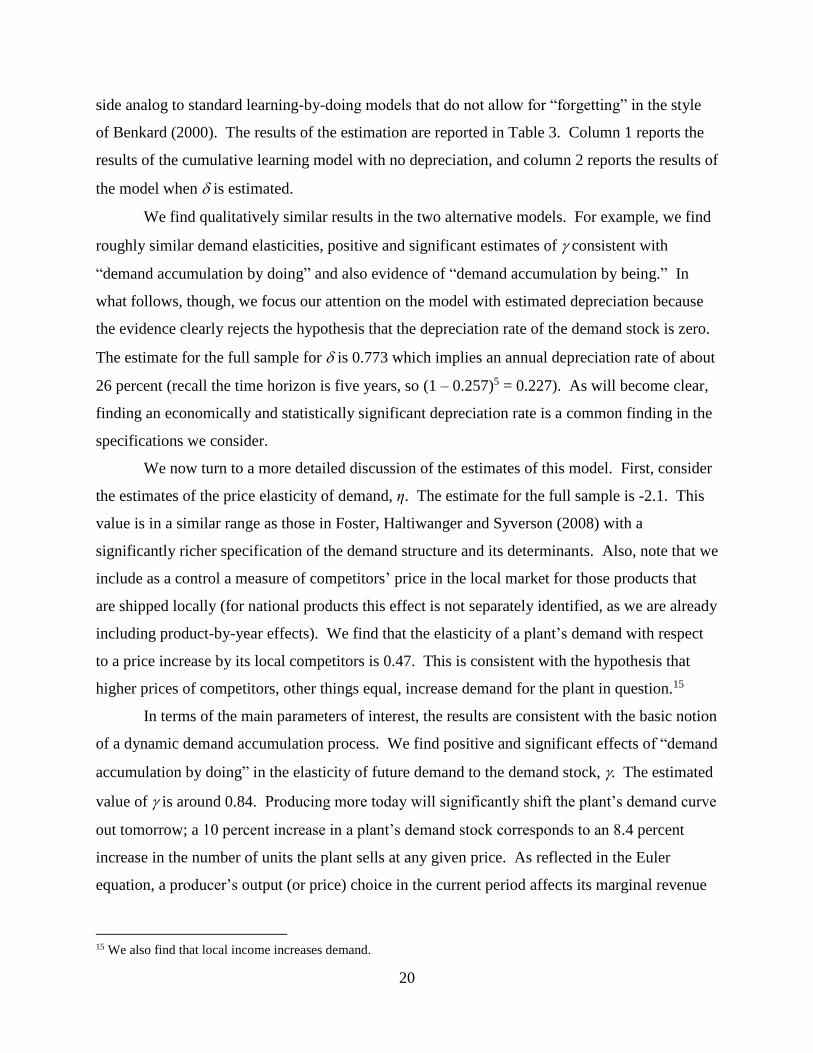
We find qualitatively similar results in the two alternative models. For example, we find
roughly similar demand elasticities, positive and significant estimates of consistent with
“demand accumulation by doing” and also evidence of “demand accumulation by being.” In
what follows, though, we focus our attention on the model with estimated depreciation because
the evidence clearly rejects the hypothesis that the depreciation rate of the demand stock is zero.
The estimate for the full sample for is 0.773 which implies an annual depreciation rate of about
26 percent (recall the time horizon is five years, so (1 – 0.257)5 = 0.227). As will become clear,
finding an economically and statistically significant depreciation rate is a common finding in the
specifications we consider.
We now turn to a more detailed discussion of the estimates of this model. First, consider
the estimates of the price elasticity of demand, η. The estimate for the full sample is -2.1. This
value is in a similar range as those in Foster, Haltiwanger and Syverson (2008) with a
significantly richer specification of the demand structure and its determinants. Also, note that we
include as a control a measure of competitors’ price in the local market for those products that
are shipped locally (for national products this effect is not separately identified, as we are already
including product-by-year effects). We find that the elasticity of a plant’s demand with respect
to a price increase by its local competitors is 0.47. This is consistent with the hypothesis that
higher prices of competitors, other things equal, increase demand for the plant in question.15
In terms of the main parameters of interest, the results are consistent with the basic notion
of a dynamic demand accumulation process. We find positive and significant effects of “demand
accumulation by doing” in the elasticity of future demand to the demand stock, . The estimated
value of is around 0.84. Producing more today will significantly shift the plant’s demand curve
out tomorrow; a 10 percent increase in a plant’s demand stock corresponds to an 8.4 percent
increase in the number of units the plant sells at any given price. As reflected in the Euler
equation, a producer’s output (or price) choice in the current period affects its marginal revenue
15 We also find that local income increases demand.

21
not just in the present period but in the future as well.
This parameter estimate can also help us get a feel for the potential return to a business
“investing” in its demand stock by lowering prices today in hopes of shifting out its demand
tomorrow. Based on the estimated price elasticity in the model with depreciation, a ten percent
price cut will increase current quantity sold by about 21 percent and current revenues by 12
percent. (This is a sizeable price deviation from one’s competitors, but not unusual. The
average within-market standard deviation of plants’ logged prices is 0.18.) The effect of this
increase in revenues on the plant’s demand in the following year diminishes with the plant’s
existing demand stock Z because a given revenue increment will have a smaller effect on larger
existing stocks. If we consider a plant whose pre-existing demand stock is of roughly equal size
to its expected revenue—that is, a young plant that would have a relatively high return to
investing in future demand—raising revenues by cutting prices ten percent would shift out next
year’s demand by about 5 percent, taking into account both depreciation and . This means the
plant will be able to sell 5 percent more units at a given price than it would otherwise.
In addition to the endogenous demand accumulation effect, we find that, having
controlled for a plant’s demand stock, “demand accumulation by being” also contributes in part
to the demand gaps across businesses of different ages. The coefficient on the young dummy is
negative and significant, while the coefficient on the medium age dummy is much smaller and
not significant. Since the omitted group is the oldest plants, the results imply exogenous demand
accumulates with age, though most of this happens by the time the plant is medium-aged. This is
qualitatively consistent with the raw demand gap patterns in Table 1, but these effects here are
much smaller than those in Table 1. This indicates that once we have accounted for endogenous
demand accumulation (and other factors), the remaining “exogenous” age gap is much smaller.
We will conduct further exercises below to gauge the quantitative implications of the estimated
demand accumulation parameters.
Remember that both of these “accumulation by doing” and “accumulation by being”
effects are estimated while controlling for the potential presence of serially correlated
unobserved demand shocks. We parameterize the persistence of these demand shocks with the
five-year AR(1) coefficient ρ, which we estimate to be about 0.22. This five-year persistence
rate corresponds to an annual rate of 0.74.
The impact of the characteristics of the owning firm on an entering plant’s initial demand

22
stock is seen in the comparison of the estimates of λ1 and λ2. The value of λ1, which
parameterizes how a plant’s initial demand stock Z is related to its physical capital stock, is 0.95,
indicating that, not surprisingly, plants with larger initial physical capital tend to have larger
starting demand stocks. The parameter also indicates that the ratio between the two types of
capital falls slightly in the plant’s size. The estimated value of λ2, which is the elasticity of a
plant’s initial demand stock to the size of the firm (in physical capital terms) relative to the
entering plant, is 0.32. This indicates that, consistent with the descriptive results seen in Table 2,
new plants of larger firms do in fact have higher initial demand stocks. A plant started by a firm
that is twice as large as another entering plant’s firm will start with about a 22 log point
(0.320*ln2 = 0.22) higher demand stock.
The table also reports the coefficient estimates for two selection controls. The coefficient
estimates on the selection controls suggest that any selection bias is relatively modest in our
sample. One estimate is statistically significant, but all are small in magnitude. The values of
the other parameter estimates are roughly similar in unreported specifications that exclude the
selection controls.
5.2. Estimates Using Local Products and Concrete Plants
To explore the consistency of our parameter estimates across the industries in our sample,
we estimate the model on two successively smaller subsamples. One uses only those plants in
local products industries (boxes, bread, concrete, and ice), and the other uses concrete plants
alone. (We choose concrete for the single-industry subsample because it has the largest number
of plants in our sample of any industry.) The results are in Table 4; column 1 reports the
estimates for the local products subsample, and column 2 reports the concrete results. We again
focus on the specification with depreciation because in both of these subsamples the estimated
rate of depreciation is far from zero.
Overall, the results for the two subsamples are qualitatively similar to the results for the
full sample, suggesting it is not overly restrictive to constrain the parameters to be the same
across all product industries. There are some quantitative differences, however, that we discuss
briefly. Demand is more own-price elastic for concrete than for the entire sample. Concrete

23
demand is also considerably more responsive to local competitors’ prices.16 The all-local-
products subsample has elasticities that are close in magnitude to those from the entire sample,
though the point estimates here are a bit larger in size.
The main parameter of interest, the elasticity of demand to the plant’s endogenously
acquired demand capital, is roughly the same in these subsamples as for the whole sample, with
estimated at about 0.8. While is similar across products, concrete has a substantially lower
depreciation rate (an implied 11 percent per year as opposed to 23 percent per year), which is
important for the demand accumulation dynamics. Combining these depreciation and price
elasticity estimates suggests that a plant that cuts prices by ten percent to invest in future demand
will raise current revenues by about 13 percent for local products and 18 percent in the concrete
subsample. This increase in sales will in turn increase the producer’s quantity demanded next
year by about 5 percent for local products and 7 percent for concrete.
We also find that the exogenous (age-related) demand accumulation process has similar
qualitative patterns as for the entire sample. There is a positive estimated demand-accumulation-
by-being effect for both local products and concrete that is mostly observed in the producer’s
transition from young to medium age. The quantitative effects are somewhat smaller in local
products than for the full sample, while the point estimate for concrete is larger.
The estimated value of λ1 is 0.97 for local products and 1.13 for concrete, which again
indicates larger plants tend to have larger starting demand stocks. For these products, the ratio
between initial demand and physical capital grows with plant size. The influence of firm size on
a plant’s initial demand stock, which is embodied in λ2, is 0.30 for local products and 0.36 for
concrete. A plant started by a firm that is twice as large as another entering plant’s firm will start
with about a 21 percent higher demand stock if the plant is in the local products industries and a
25 percent higher demand stock if the plant is in the concrete industry.
Again, selection does not appear to be quantitatively important. All of the four inverse
Mills ratios are small, and estimating the model without including any selection correction terms
(not shown) yielded similar estimates of the other parameters.
5.3. Interactions with Multi-Plant Firm Status
16 The estimated price elasticity of demand for concrete is somewhat lower than that reported in Foster, Haltiwanger
and Syverson (2008).

24
A striking result from the descriptive exercises in Section 3 is that entrants that are part of
larger, multi-plant firms enter with a higher demand stock than those in smaller or single-plant
firms. This was confirmed in the estimated model above as well, as the elasticity of initial
demand stock to the ratio of the firm’s size to the entering plant’s size, λ2, was positive.
However, it was less clear in the descriptive results whether the rate of convergence of
idiosyncratic demand levels was faster for young plants in multi-plant firms than those in small
firms. To examine this issue through the lens of our model, we also estimate a specification that
interacts an indicator for plants that are owned by a multi-plant firm with the model’s parameters
(except for λ1 and λ2, which already incorporate such multi-unit firm effects).
The results for both the entire sample (column 1) and the local-products-only sample
(column 2) are shown in Table 5 (for the sake of brevity, we do not report results for ready mix
concrete separately – they are similar to those for the local products sample). To interpret the
results in this table, the “main effects” provide estimates for single-unit plants, and the
interactions with the MU dummy show whether MU plants have a significant differential from
the single-unit plants (thus the total MU coefficient is the sum of the main and interaction
effects).
The interactions between the multi-unit indicator and in both samples are small and
statistically insignificant, so both single-unit and multi-unit producers see similar responses of
demand to their accumulated demand stock. On the other hand, estimated depreciation is lower
and demand is slightly more elastic for multi-unit plants, so a given sized price cut could yield a
slightly greater and longer lasting bump in accumulated demand.
The “accumulation by being” effect is significantly stronger for multi-unit than single-
unit plants. This can be interpreted as suggesting that the residual unexplained component of the
patterns observed in Table 2 is larger for multi-unit plants. We return to this issue below.
One of the largest differences between single- and multi-unit producers in Table 2 is the
difference in the intercepts. This is captured here by permitting the presence and size of the
parent firm at the time of entry of the plant to contribute to the demand stock. Given the large
estimated coefficients for λ2 (0.36 for the full sample and 0.38 for local products), there is a
substantial level shift in the demand curve for establishments that are part of multi-unit firms.
Multi-unit plants have initial firm-level capital stocks that are on average about 1.9 times that of
the median entering establishment. Using the full-sample estimates, this implies such
25
establishments start with demand stocks that are 23 log points (0.363*ln1.9 = 0.23) higher.
5.4. Evolution of Demand by Age: Exogenous versus Endogenous Demand Accumulation
To further quantify the contribution of exogenous versus endogenous demand
accumulation to the observed evolution of demand across plant ages, we return to the metric used
in Table 1. In particular, we use the estimated coefficients from our model along with the actual
data to compute the implied levels of both demand components for every plant-year observation
in our sample. We then derive the type of statistics reported in Table 1 for each of these
computed components.
We compute the component of demand from the exogenous demand accumulation
(“accumulation by being”) using the estimates of age dummy variables in Tables 3 and 4. For
the endogenous demand component (“accumulation by doing”), we first compute Zt for every
plant in the sample using our data on plants’ revenues and capital stocks along with the estimates
of λ1, λ2 and . We then combine the estimated Zt with our estimate of to compute the
endogenous demand accumulation component for every plant-year observation.
Table 6 reports the results of these exercises. The top panel shows the results for the full
sample, the middle panel for local products plants, and the bottom panel for concrete plants. The
age categories that we use in this exercise are similar to those used earlier, but now we have
subsumed “Entrants” into the “Young” category for two reasons. First, the model only yields
estimates of the exogenous demand accumulation component for these same young and medium
categories relative to older plants.17 Second, this grouping of ages implies that all counterfactual
estimates of endogenous demand accumulation component reflect actual past sales rather than
just our estimated demand stock initialization.
Because we use somewhat collapsed age categories and capital stock data are not
available for all plants used in Table 1, the first row in each of the panels of Table 6 repeats
exactly the type of analysis done in Table 1 for this restricted sample. As in Table 1, these
estimated coefficients are from a regression of plant-level idiosyncratic demand on age dummies
17 While the learning by being component for the young reflects plants between 5-9 years old, one can obtain for a
plant of any age an estimate of the contribution of all components of demand other than the endogenous demand
accumulation at any age by taking the difference between the overall producer-level demand observed in the data
and the endogenous demand accumulation component. This difference includes the accumulation by being
component but also other components like the unobserved persistent demand component θ.
26
and industry-year fixed effects. The demand patterns for each panel in Table 6 are similar
qualitatively and quantitatively to those in Table 1. Young and Medium aged plants have much
lower demand than old plants, and convergence is slow.
Our model lets us decompose this overall demand residual into multiple components.18
The age patterns for the endogenous accumulation component are reported in the second row of
each panel. For the full sample, the endogenous accumulation component essentially explains all
of the 29 log point demand gap between medium and old plants. It cannot fully explain young
plants’ demand disadvantage, however, falling about 30 log points short. The accumulation by
being component closes part of this gap, predicting a 14 log point gap between young plants and
industry incumbents. There is only a small (2 log point) predicted accumulation by being during
plants’ movement from medium to old age. These results imply that most of the overall demand
shock patterns for our sample plants are accounted for by endogenous accumulation of demand
rather than exogenous components.
Results for local and concrete plants are similar. The endogenous accumulation
component in all cases is much lower for young plants than old plants (40 log points lower for
local product plants and 33 log points lower for concrete plants), and there is only slow
convergence. Accumulation by being accounts for a larger share of demand growth in the
concrete subsample than in either the overall or local products sample—in concrete, about 30
percent of the 57 log point demand gap between young and old plants is explained by exogenous
accumulation—but in every case the majority of demand accumulation occurs via the
endogenous channel.
6. Alternative Explanations and Robustness Checks
In this section, we attempt to address two basic concerns that we anticipate readers might
have and provide some additional robustness checks. The first basic concern is relatively minor
and is addressed in the first subsection. It regards whether our idiosyncratic demand measures—
the ones used in Sections 1 and 2 to motivate our model—do actually reflect a plant’s demand
state in a given period. In the second subsection we address the more serious concern that we
have allowed only one channel for dynamics in our model, demand accumulation. If a plant’s
18 The two components we report do not add up to the total because there are other factors—in particular, the serially
correlated demand component θ — that enter into the demand equation.

27
management takes into account other dynamic factors when making decisions, we would
mistakenly measure these other factors’ influence as a response to our specified demand
dynamics. We agree that both of these concerns are theoretically valid and that they almost
surely have some empirical relevance. However, we believe that the setting of the problem and
the way we estimate the model substantially mitigates such concerns.
6.1. What Do Our Idiosyncratic Demand Stock Measures Reflect?
Our idiosyncratic demand stock measures reflect the cross-plant variation in units of
output sold that is, by construction, purged of the effects of plants’ physical production costs. If
plant A both sells more output and has a higher idiosyncratic demand measure than plant B, plant
A’s high sales are not simply the result of plant A having lower prices because it has low costs.
Plant A would sell more than plant B even if it were charging the same price. Regardless of any
other measurement issues with these idiosyncratic demand measures, by construction they reflect
quantities sold that are orthogonal to plants’ physical production costs as captured in our TFPQ
measures.
That said, there are other measurement issues that might lead these demand measures to
capture other factors. Primary among these is the issue of capacity utilization. The demand
measure is based on the quantity (i.e., the number of units) the plant sells. Our descriptive
results could be explained by an alternative story where new plants are built to be the same size
(at least in terms of capital) as older plants in their industry, but they look like they have low
demand because they are slow to be fully utilized. In this case, firms design plants to be “grown
into”; they have the physical infrastructure to handle output levels typical of older incumbents,
but are only lightly utilized at first.
We have two responses to this possibility. First, this story is not inconsistent with our
theorized demand-accumulation process. New plants may operate at low utilization levels
precisely because their demand stock is low. As they accumulate a customer base or build
supplier-consumer relationship capital in one form or another, their output slowly grows to fit the
capacity of the plant. Why a firm might find it optimal to build an initially oversized plant will
depend on the size of capital adjustment costs (more on this below), but our idiosyncratic
demand measures could still reflect the demand accumulation process in this case.
Second, the data do not support this sort of capacity utilization pattern. We cannot
28
measure capacity utilization directly, but we can construct two good utilization proxies for each
plant: the capital-stock-to-output ratio, and the energy-use-to-capital-stock ratio. The former
measures whether plants’ production quantities are proportional to their reported capital stocks.
The latter relates a common proxy in the literature for the flow of capital services, energy use, to
reported capital stock measures. For capacity utilization to explain the demand patterns
discussed above, younger plants would have to have systematically higher capital-to-output
levels and lower energy-to-capital ratios than older plants.
Table 7 presents the utilization patterns for our sample. The table replicates the
specification of Table 2, except using the capacity utilization proxies as the dependent variables
(each is used in a separate regression). The results indicate mixed patterns of utilization across
plant ages, but even in those cases where utilization moves in the right direction, there is not
nearly enough quantitative movement to explain our patterns above. When measured by capital-
to-output ratios, as in the top half of the table, utilization is actually higher at younger single-unit
plants than older ones (that is, their capital-output ratio rises with age). This pattern is reversed
among plants in multi-unit firms, but there the total utilization difference between new and old
plants is about 4.5 percent. Thus it can explain only about 10 percent of the measured demand
gap. Similar patterns hold, though with less monotonicity over age groups, for the results using
energy-capital ratios to measure utilization. Utilization is actually higher for new single-unit
plants than old ones and only about five percent lower in the case of new multi-unit plants.
6.2. Other Dynamic Forces
A more serious concern is that the demand accumulation process is the only source of
dynamics in our model. If plant decisions are made in response to additional dynamic forces, our
estimation will interpret such actions through a demand accumulation lens, not the true economic
process driving the decisions. We envision three broadly-defined alternative dynamic factors that
our plants might face: a dynamic process in physical productivity (i.e., shifts in At over time),
financing constraints, and capital adjustment costs. We address each of these possibilities in
turn.
Physical productivity dynamics would involve predictable moves in a plant’s At.
Certainly, many have documented that plants experience persistent productivity shocks (see the
papers in Bartelsman and Doms (2000), for example). Indeed, a possible source of such

29
movements, though certainly not the only one, would be a traditional learning by doing
mechanism.
However, Table 1 makes clear that the patterns in the data are not consistent with supply-
side learning by doing—this is, after all, a basic motivation of our investigation. This suggests
that physical productivity dynamics are less of a concern in our context. While individual plants
in our sample no doubt experience some persistent, predictable At shocks, the results in Table 1
indicate these do not have much of a systematic correlation with plant age. Certainly they do not
hold clear patterns over the 15+ year growth horizons we are attributing to demand movements.
The quantitative movements in TFPQ that do exist across ages are very small relative to the
demand variation that is our focus. So while we agree that physical productivity dynamics exist
and can play important roles in explaining certain plant-level behaviors, we see no evidence that
they are playing a major role in explaining plant-level choices of the type and horizon that we are
using to identify the demand accumulation process parameters.
Capital constraints can create dynamics because constrained businesses may accumulate
financial capital in one period in order to loosen a constraint on expansion in the future. They
would also be a reason for new businesses starting small, since if barriers to obtaining credit
exist, it is plausible that new producers would be more likely to face them than would more
established businesses.
We do not have plant-specific information on credit access or costs of capital, so we
cannot directly test for the presence of credit constraints. However, we can look at measured
demand levels and growth for different types of firms that might be expected to vary
systematically in the extent to which they are credit constrained. The most applicable exercise
that we have done in this regard is the breakout of demand patterns for plants of multi-unit firms
in Table 2. Plants in these larger firms expectedly face lower credit constraints than do single-
unit plant/firms either through easier access to external funding or more flexibility in being able
to tap into internal capital. And while these multi-unit plants tend to be larger, they still exhibit
the very slow convergence in measured demand levels seen among plants of smaller firms. This
seems inconsistent with a world where the measured patterns primarily embody financing
constraints instead of long-horizon demand accumulation.
Capital adjustment costs, even in the absence of any credit constraints, could produce
qualitative patterns similar to those we see in the data. Plants may respond slowly to even long-

30
run demand shifts if it is costly for them to change the size of their business. In such a case, the
slow output growth we observe may not reflect gradual demand accumulation, but rather a
gradual expansion in the face of persistently high demand.
We do in fact expect that capital adjustment costs play a role in plants’ decisions—after
all, most capital is not rented via short-term agreements, and there are several potential frictions
in capital sales markets. However, the estimates from the literature on the size of capital
adjustment costs suggest that they cannot quantitatively explain the patterns we document. Even
assuming adjustment costs at the high range of estimates, the time it would take for a plant to
close the output gap (assuming capital utilization rates are constant over time) observed in Table
1 is relatively short. For example, the capital adjustment costs estimates in Cooper and
Haltiwanger (2006), which were estimated using similar plant-level data to our own sample
(except on an annual frequency and spanning the entire manufacturing sector) suggest plant size
could fully adjust to the observed output gap in less than one year. Even some of the larger
estimates of capital adjustment costs, like those in Gilchrist and Himmelberg (1995), imply the
capacity adjustment will fully occur in only three years.
Hence it seems unlikely that capital adjustment costs could explain all, or even most, of
the 15+ years it takes for plants in our sample to close their measured idiosyncratic demand gap.
Much as with physical productivity dynamics discussed above, therefore, we expect that while
capital adjustment costs are important in some contexts, they do not have the quantitative impact
necessary to explain the long-horizon demand-growth patterns we observe in the data.
6.3. Robustness Checks
We discuss briefly a number of robustness checks that we conducted on our analysis in
this subsection. Relevant estimates for these robustness checks are reported in the appendix.
First, we investigated the sensitivity of our results to permitting a different discount factor
. The results reported in Tables 3-6 reflect an assumed annual discount factor of 0.98. Figure
A.1 shows how the key parameters of and vary for discount factors ranging between 0.96 and
0.98. The estimates are quite robust across this range. We focus on these two parameters
because they are the critical estimates for the endogenous demand accumulation, but we also
found (results available upon request) that other estimated parameters are also robust over this
range of .

31
Second, we explored refinements of the role of being part of a multi-unit firm upon entry.
The main results imply that plants entering as part of a multi-unit firm have significantly higher
initial demand stocks. To explore this mechanism further, we considered whether this is tied to
the nature of the overlap of a new plant’s activity with its parent firm. Specifically, we tested
whether the entering plant’s initial demand was higher if its owning firm had experience
operating other plants in the same geographic area (using the BEA Economic Area definition of
geographic areas) and industry (using 4-digit SIC industries). We found some evidence in favor
of this conjecture as reported in Table A.3. For the sake of brevity, we focus on the local plants
sample where these effects are most likely to be relevant. As shown in Table A.3, a plant started
by a firm with activity in the same geographic area has statistically significant higher initial
demand. But we also find that the contribution of initial demand capital from the firm’s plants
that are not part of the same geography remains significant. This suggests that the demand
advantage of being part of a multi-unit does not stem simply from the activity of the firm’s other
plants in the same geographic market. For the case of industry, we find that the point estimates
for the parent’s contribution coming from both the same and other industries are both positive,
but when both are included neither is individually statistically significant. When we combine the
effects (as in Table 4), the parents contribution is positive and statistically significant.
A third set of refinements we conducted was to allow some systematic variation in the
model’s parameters across industries by permitting the estimated parameters to vary with
observed characteristics of our sample products. We already saw in Tables 3 and 4 that while the
results are qualitatively similar across our sample products, there is some quantitative variation
in the parameter estimates across the full sample, the subsample of local product producers, and
concrete plants. We considered allowing the parameters to vary with several alternative product
characteristics, and in particular the nature of the downstream industries that purchase our
sample products (we identified these downstream industries using the input-output matrix). We
conjectured, for example, that producers who sell to downstream industries with more turnover
of producers would face weaker incentives for demand stock accumulation, while those selling to
more concentrated downstream industries would face stronger incentives. We found little
evidence in favor of these conjectures (see Table A.4 for details).
7. Conclusion

32
New businesses (and extensions of existing businesses built in new markets) are almost
invariably smaller than established businesses in the same market, and this size gap closes slowly
with time. An active literature spanning several fields has hypothesized that these patterns
reflect demand dynamics. We have used a unique dataset of U.S. manufacturing plants to
empirically explore this hypothesis. We first demonstrate that these average size gaps across
plants of different ages are in fact the result of demand rather than supply-side cost
fundamentals. Next, after descriptively characterizing patterns of idiosyncratic demand across
plants, we build and estimate a dynamic model of plant expansion in the presence of a demand
stock that can grow both exogenously over time and endogenously in the response to the plant’s
investments. We find that the model can explain a considerable portion of the relationship
between plant age and size, even in our sample of physically homogeneous, commodity-like
products. The data also indicate that the active (endogenous) “demand accumulation by doing”
mechanism plays a greater role in explaining the small size and slow growth of new plants than
does passive (exogenous) “demand accumulation by being,” though both channels matter. We
also characterize cross-sectional differences in demand levels within similarly aged plants,
showing for example that entering plants owned by firms that already operate other plants
elsewhere appear to enjoy some spillover demand capital benefits from their corporate parent.
Our results imply that, even in commodity-like product industries, entry is difficult. It
takes a long time for new businesses, even those owned by large firms, to reach a point where
they have built enough relationship-specific capital with their potential customers to expect (at
the same price) to sell the same amount of output as do their more established competitors. This
buttresses the recent literature pointing towards the importance of idiosyncratic demand factors
in explaining the fortunes of businesses, and it has implications for the nature of competition in
markets, firm valuations, the evolution of industries, and the prospects for exporting in new
markets.
A clear next step that researchers can take based on these results is to explore the
particular mechanisms that underlie the endogenous and exogenous demand accumulation
processes in our model. Several questions present themselves: How much of this reflects brand
effects, or reputation, or other aspects of buyer supplier relationships? Does the specific
mechanism at work differ across markets, and how if so? Given this, is it natural that active
accumulation processes quantitatively dominate passive processes? What affects the extent to

33
which a firm’s demand capital spills over to its newly built or newly acquired plants? These
questions and others strike us as being important for gaining a deeper understanding of the
processes at work in our empirical results.
References
Ábrahám, Árpád and T. Kirk White. “The Dynamics of Plant-Level Productivity in U.S.
Manufacturing.” Center for Economic Studies Working Paper 06-20, 2006.
Aguirregabiria, Victor. “Estimation of Dynamic Programming Models with Censored Dependent
Variables.” Investigaciones Economicas, 21(2), 1997, 167-208.
Arkolakis, Costas. “Market Penetration Costs and the New Consumers Margin in International
Trade.” Journal of Political Economy, 2010, 118(6), 1151-1199.
Alonso-Borrego, César. “Demand for Labour Inputs and Adjustment costs: Evidence from
Spanish Manufacturing Firms, Labour Economics, 1998, 475–497.
Asplund, Marcus and Volker Nocke. “Firm Turnover in Imperfectly Competitive Markets.”
Review of Economic Studies, 73(2), 2006, 295-327.
Bar-Isaac, Heski and Steven Tadelis. “Seller Reputation.” Foundations and Trends in
Microeconomics, 4(4), 2008, 273-351.
Bartelsman, Eric J. and Mark Doms. “Understanding Productivity: Lessons from Longitudinal
Microdata.” Journal of Economic Literature, 38(3), 2000, 569-95.
Benkard, C. Lanier. “Learning and Forgetting: The Dynamics of Aircraft Production.” American
Economic Review, 90(4), 2000, 1034-54.
Brown, J. David, John S. Earle, and Almos Telegdy. “The Productivity Effects of Privatization:
Longitudinal Estimates from Hungary, Romania, Russia, and Ukraine.” Journal of
Political Economy, 114(1), 2006, 61-99.
Cabral, Luís M B, and José Mata. “On the Evolution of the Firm Size Distribution: Facts and
Theory." American Economic Review, 93(4), 2003, 1075–1090.
Caminal, Ramon and Xavier Vives. “Price Dynamics and Consumer Learning.” Journal of
Economics and Management Strategy, 8(1), 1999, 95-131.
Caves, Richard E. “Industrial Organization and New Findings on the Turnover and Mobility of
Firms.” Journal of Economic Literature, 36(4), 1998, 1947-82.
Cooper, Russell W. and John C. Haltiwanger. “On the Nature of Capital Adjustment Costs.”
Review of Economic Studies, 73(3), 2006, 611-33.

34
Das, Sanghamitra, Mark J. Roberts, and James R. Tybout. “Market Entry Costs, Producer
Heterogeneity, and Export Dynamics.” Econometrica, 75(3), 2007, 837-73.
De Loecker, Jan. “Product Differentiation, Multiproduct Firms, and Estimating the Impact of
Trade Liberalization on Productivity.” Econometrica, 79(5), 2011, 1407-51.
Dinlersoz, Emin and Mehmet Yorukoglu. “Information and Industry Dynamics.” US Census
Bureau Center for Economic Studies Paper No. CES-WP-10-16, 2010.
Dixit, Avinash K. and Robert S. Pindyck. Investment under Uncertainty. Princeton, NJ:
Princeton University Press, 1994.
Drozd, Lukasz A. and Jaromir B. Nosal. “Understanding International Prices: Customers as
Capital.” American Economic Review, 102(1), 2012, 364-95.
Dunne, Timothy, Mark J. Roberts, and Larry Samuelson. “Patterns of Firm Entry and Exit in
U.S. Manufacturing Industries.” RAND Journal of Economics, 19(4), 1988, 495-515.
Dunne, Timothy, Mark J. Roberts, and Larry Samuelson. “Firm Entry and Postentry
Performance in the U.S. Chemical Industries.” Journal of Law and Economics, 32(2) Part
2, 1989a, S233-71.
Dunne, Timothy, Mark J. Roberts, and Larry Samuelson. “The Growth and Failure of U.S.
Manufacturing Plants.” Quarterly Journal of Economics, 104(4), 1989b, 671-98.
Eslava, Marcela, John Haltiwanger, Adriana Kugler and Maurice Kugler. “Plant Survival,
Market Fundamentals and Trade Liberalization.” Mimeo, 2008.
Fishman, Arthur and Rafael Rob. “Consumer Intertia, Firm Growth and Industry Dynamics.”
Journal of Economic Theory, 109(1), 2003, 24-38.
Fishman, Arthur and Rafael Rob. “Is Bigger Better? Customer Base Expansion through Word‐of‐Mouth Reputation.” Journal of Political Economy, 113(5), 2005, 1146-1162.
Foster, Lucia, John Haltiwanger, and Chad Syverson. “Reallocation, Firm Turnover, and
Efficiency: Selection on Productivity or Profitability?” American Economic Review,
98(1), 2008, 394-425.
Gilchrist, Simon and Charles P. Himmelberg. “Evidence on the Role of Cash Flow for
Investment.” Journal of Monetary Economics, 36(3), 1995, 541-72.
Gourio, Francois and Leena Rudanko. “Customer Capital.” NBER Working Paper No. 17191,
2011.
Hopenhayn, Hugo. “Entry, Exit, and Firm Dynamics in Long Run Equilibrium.” Econometrica,
35
60(5), 1992, 1127-1150.
Jovanovic, Boyan. “Selection and Evolution of Industry.” Econometrica, 50(3), 1982, 25-43.
Kee, Hiau Looi and Kala Krishna. “Firm-Level Heterogeneous Productivity and Demand
Shocks: Evidence from Bangladesh.” American Economic Review Papers and
Proceedings, 98(2), 2008, 457-62.
Klepper, Steven. “Firm Survival and the Evolution of Oligopoly.” The RAND Journal of
Economics, 33(1), 2002, 37-61.
Luttmer, Erzo G. J. “On the Mechanics of Firm Growth.” Review of Economic Studies, 78(3),
2011, 1042-1068.
Melitz, Marc J. “The Impact of Trade on Intra-Industry Reallocations and Aggregate Industry
Productivity.” Econometrica, 71(6), 2003, 1695-1725.
Pakes, Ariel. “Dynamic Structural Models: Problems and Prospects. Mixed Continuous
Discrete Controls and Market Interactions” in C. Sims (ed.) Advances in Econometrics.
Sixth World Congress. Vol 2. 1994, Cambridge University Press.
Pakes, Ariel and Richard Ericson. “Empirical Implications of Alternative Models of Firm
Dynamics.” Journal of Economic Theory, 79(1), 1998, 1-45.
Perla, Jesse. “Product Awareness and the Industry Life Cycle.” Working Paper, 2013.
Radner, Roy. “Viscous Demand.” Journal of Economic Theory, 112(2), 2003, 189–231.
Semykina, A. and Wooldridge, J. M. “Estimation of Dynamic Panel Data Models with Sample
Selection.” Journal of Applied Econometrics, 28(1), 2013, 47–61.
Syverson, Chad. “What Determines Productivity?” Journal of Economic Literature, 49(2), 2011,
326-65.
Troske, Kenneth R. “The Dynamic Adjustment Process of Firm Entry and Exit in Manufacturing
and Finance, Insurance, and Real Estate.” Journal of Law and Economics, 39(2), 1996,
705-35.
U.S. Bureau of Economic Analysis. “Redefinition of the BEA Economic Areas.” Survey of
Current Business, February 1995, 75-81.
Vella, Francis. “Estimating Models with Sample Selection Bias: A Survey.” Journal of Human
Resources, 33(1), 1998, 127-169.

36
Table 1. Evolution of Productivity and Demand across Plant Ages
Variable
Plant Age Dummies
Entrant Young Medium Exiter
Productivity
(TFPQ)
0.013
(0.005)
0.004
(0.006)
-0.004
(0.006)
-0.018
(0.005)
Demand
-0.550
(0.022)
-0.397
(0.024)
-0.316
(0.026)
-0.339
(0.021)
Note: Table shows the coefficients on indicator variables for exiting, entering, and continuing plants of two age
cohorts (“young” and “medium” establishments) when we regress plant-level productivity and demand levels on
these indicators and a full set of product-year fixed effects. The excluded category is “old” plants. The sample
includes roughly 17,000 plant-year observations from the 1977, 82, 87, and 92 Census of Manufactures. Standard
errors, clustered by plant, are in parentheses. This table is similar to Table 5 in Foster, Haltiwanger, and Syverson
(2008) but uses a measure of demand shock that is more consistent with that used in subsequent exercises and a
smaller sample (excludes plants manufacturing gasoline from the analysis).
Table 2. Evolution of Demand across Plant Ages—Interactions with Firm’s Multi-Unit Status
Variable
Plant Age Dummies
Entrant Young Medium Old Exiter
Demand
-0.318
(0.034)
-0.176
(0.035)
-0.150
(0.038) Excl.
-0.183
(0.031)
Demand x MU firm 0.106
(0.038)
0.132
(0.041)
0.237
(0.045)
0.530
(0.026)
-0.283
(0.042)
Note: Table expands the analysis of Table 1by allowing plant age effects to vary with the multi-unit (MU) status of
the plant’s owning firm. The excluded category is “old” plants that are part of a single-unit firm. N is roughly
17,000 plant-year observations. Standard errors, clustered by plant, are in parentheses.

37
Table 3. Estimated Coefficients for Cumulative Learning and Depreciation Models
Parameter Cumulative
Learning
Learning
with
Depreciation
(elasticity of future demand to the demand stock)
0.399
(0.036)
0.841
(0.014)
-
(price elasticity of demand)
-2.312
(0.166)
-2.124
(0.080)
Young dummy
(demand shift for entering and young plants)
-0.300
(0.053)
-0.140
(0.043)
Medium age dummy
(demand shift for medium-aged plants)
-0.087
(0.038)
-0.022
(0.026)
(persistence of exogenous demand shocks )
0.899
(0.053)
0.219
(0.088)
(demand depreciation rate)
0.773
(0.033)
1
(elasticity of initial demand to plant’s own K) 1.578
(0.059)
0.954
(0.035)
2
(elasticity of initial demand to ratio of firm’s K to plant’s K) 0.328
(0.110)
0.320
(0.050)
Competitor’s Price (local products only)
0.349
(0.128)
0.468
(0.078)
Selection Correction, Demand Equation
0.027
(0.025)
-0.033
(0.019)
Selection Correction, Euler Equation
-0.001
(0.006)
0.018
(0.006)
Notes: Joint Demand and Euler Estimation is based on joint estimation of equations (2b) and (7c) for the entire
sample. Demand equation also includes year dummies (not reported) and control for local demand (local BEA
economic area income). “Young” is the definition that subsumes entrants. The omitted age group is mature plants.
The instruments for demand equation include log(TFPQ), lagged revenues (up to six lags), lagged price, local
income, age and year dummies. Instruments for Euler equation include lagged revenue (up to six lags), lagged
cost/revenue ratios (up to two lags), lagged price (up to two lags), and age dummies. Standard errors are in
parentheses.
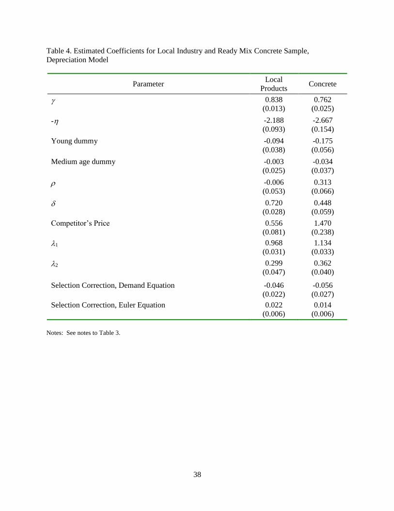
38
Table 4. Estimated Coefficients for Local Industry and Ready Mix Concrete Sample,
Depreciation Model
Parameter Local
Products Concrete
0.838
(0.013)
0.762
(0.025)
-
-2.188
(0.093)
-2.667
(0.154)
Young dummy
-0.094
(0.038)
-0.175
(0.056)
Medium age dummy
-0.003
(0.025)
-0.034
(0.037)
-0.006
(0.053)
0.313
(0.066)
0.720
(0.028)
0.448
(0.059)
Competitor’s Price 0.556
(0.081)
1.470
(0.238)
1
0.968
(0.031)
1.134
(0.033)
2
0.299
(0.047)
0.362
(0.040)
Selection Correction, Demand Equation
-0.046
(0.022)
-0.056
(0.027)
Selection Correction, Euler Equation
0.022
(0.006)
0.014
(0.006)
Notes: See notes to Table 3.

39
Table 5. Estimated Coefficients for Learning with Depreciation Model, Interactions with Multi-
Plant Firm Status
Parameter Entire Sample Local Products
0.779
(0.028)
0.757
(0.027)
-2.648
(0.148)
-2.956
(0.206)
Young dummy 0.029
(0.068)
-0.012
(0.061)
Medium age dummy 0.049
(0.048)
0.021
(0.046)
0.483
(0.090)
0.256
(0.091)
1 1.108
(0.027)
1.045
(0.026)
2 0.363
(0.038)
0.375
(0.034)
0.580
(0.056)
0.716
(0.049)
Competitor’s Price 0.678
(0.131)
1.033
(0.196)
*MU -0.007
(0.031)
0.044
(0.030)
*MU -0.258
(0.112)
-0.611
(0.216)
Young dummy*MU -0.281
(0.081)
-0.199
(0.076)
Medium age dummy*MU -0.125
(0.060)
-0.062
(0.057)
*MU 0.069
(0.124)
0.051
(0.115)
*MU -0.171
(0.062)
-0.212
(0.058)
Competitor’s Price*MU -0.287
(0.115)
-0.629
(0.214)
Selection Correction, Demand
-0.014
(0.021)
-0.014
(0.021)
Selection Correction, Euler Equation
0.001
(0.005)
0.001
(0.005)
Notes: See notes for Table 3 above. “MU” is an indicator variable equal to one if the plant is owned by a multi-unit
(multi-plant) firm.

40
Table 6. Evolution of Demand across Plant Ages— Endogenous Learning vs. Learning By Being
Effects
Variable Young Medium Old
All Plants
Demand
-0.573
(0.020)
-0.285
(0.029)
Excl.
Endogenous Accumulation
(Accumulation by Doing)
-0.280
(0.017)
-0.277
(0.025)
Exogenous Accumulation
(Accumulation by Being)
-0.140
(0.043)
-0.022
(0.026)
Local Product Plants
Demand
-0.571
(0.020)
-0.284
(0.029)
Excl.
Endogenous Accumulation
(Accumulation by Doing)
-0.401
(0.017)
-0.280
(0.025)
Exogenous Accumulation
(Accumulation by Being)
-0.094
(0.038)
-0.003
(0.025)
Concrete Plants
Demand
-0.572
(0.021)
-0.287
(0.030)
Excl.
Endogenous Accumulation
(Accumulation by Doing)
-0.326
(0.017)
-0.238
(0.025)
Exogenous Accumulation
(Accumulation by Being)
-0.175
(0.056)
-0.034
(0.037)
Notes: Results are based on the estimates from Tables 3 and 4, respectively. Demand is computed as the difference
between (log) output and the price determinants of demand. The endogenous learning effect is computed from the
evolution of the demand capital for each plant using the estimated parameters for 𝛾and 𝛿. The learning by being
effects are repeated from Tables 3 and 4 from the estimated Young and Medium age dummies. The omitted group is
“old” establishments.

41
Table 7. Capacity Utilization Patterns Across Plant Ages and Multi-Unit Status
Capacity
Utilization
Measure Variable
Plant Age Dummies
Entrant Young Medium Old Exiter
Capital
Utilization -0.110
(0.019)
-0.086
(0.020)
-0.042
(0.022) Excl.
-0.022
(0.018)
Utilization x
MU firm
-0.077
(0.021)
-0.087
(0.023)
-0.099
(0.025)
-0.111
(0.015)
0.055
(0.024)
Energy
Utilization 0.090
(0.029)
-0.021
(0.031)
-0.057
(0.033) Excl.
0.074
(0.027)
Utilization x
MU firm
-0.070
(0.033)
0.012
(0.035)
-0.003
(0.039)
-0.022
(0.023)
-0.017
(0.036)
Note: Table estimates the same specification as Table 2, except now uses as the dependent variable two different
plant-level proxies for capacity utilization, hence showing patterns of plant utilization over age and plant multi-unit
status. The two proxies are the log of the capital stock to output ratio (“Capital”) and the log of energy use to
equipment capital ratio (“Energy’). N = roughly 17,000 plant-year observations. Standard errors are in parentheses.

42
Appendix A.1. Defining Our Products
The precise definitions of our ten products are listed below (with 7-digit product codes in parentheses).
Boxes is defined as the sum of boxes classified by their end use and boxes classified by their materials. Boxes
classified by end use are: food and beverages (2653012), paper and allied products (2653013), carryout boxes for
retail food (2653014 category starts in 1987) glass, clay, and stone products (2653015), metal products, machinery,
equipment, and supplies except electrical (2653016), electrical machinery, equipment, supplies, and appliances
(2653018), chemicals and drugs, including paints, varnishes, cosmetics, and soap (2653021), lumber and wood
products, including furniture (2653029), and all other ends uses not specified above (2653029 in 1977 and 1982,
2653030 in 1987). Boxes classified by their materials are: solid fiber (2653051), corrugated paperboard in sheets
and rolls, lined and unlined (2653067), and corrugated and solid fiber pallets, pads and partitions (2653068). The
physical data for boxes is measured in short tons.
Bread is defined as one 7-digit product, white pan bread (2051111), until 1992 when it was split into two products
white pan bread, except frozen (2051121) and frozen white pan bread (2051122). The physical data for bread is
measured in thousands of pounds.
Carbon Black is defined as one 7-digit product, carbon black (2895011 in 1977, 2895000 thereafter). The physical
data for carbon black is measured in thousands of pounds.
Coffee is the sum of whole bean (2095111), ground and extended yield (2095117 and 2095118 in 1982 and 2095115
thereafter), and ground coffee mixtures (2095121). The physical data for coffee is measured in thousands of pounds.
Concrete is defined as one 7-digit product, ready-mix concrete (3273000), over our entire sample. Some of the
products coded as 3237300 in 1987 were in fact census balancing codes and thus were deleted from our sample. The
physical data for concrete is measured in thousands of cubic yards.
Flooring is defined as one 7-digit product, hardwood oak flooring (2426111), over our entire sample. The physical
data for flooring is measured in thousands of board feet.
Block Ice is defined as one 7-digit product, can or block ice (2097011), over our entire sample. The physical data
for block ice is measured in short tons.
Processed Ice is defined as one 7-digit product, cubed, crushed, or other processed ice (2097051), over our entire
sample. The physical data for processed ice is measured in short tons.
Plywood is defined as one 7-digit product, hardwood plywood (2435100), over 1977-1987. Starting in 1992,
plywood is the sum of veneer core (2435101), particleboard core (2435105), medium density fiberboard core
(2435107), and other core (2435147). The physical data for plywood is measured in thousands of square feet
surface measure.
Sugar is defined as one 7-digit product, raw cane sugar (2061011), over our entire sample. The physical data for
sugar is measured in short tons.
A.2. Measurement of input levels and input elasticities in the TFP indexes.
Labor inputs are measured as plants’ reported production-worker hours adjusted using the method of Baily,
Hulten and Campbell (1992). This involves multiplying the production-worker hours by the ratio of total payroll to
payroll for production workers. Prior work has shown this measure to be highly correlated with Davis and
Haltiwanger’s (1991) more direct imputation of nonproduction workers, which multiplies a plant’s number of
nonproduction workers by the average annual hours for nonproduction workers in the corresponding two-digit

43
industry calculated from the CPS. Capital inputs are plants’ reported book values for their structure and equipment
capital stocks deflated to 1987 levels using sector-specific deflators from the Bureau of Economic Analysis. The
method is detailed in Foster, Haltiwanger and Krizan (2001). Materials and energy inputs are simply plants’
reported expenditures on each deflated using the corresponding input price indices from the NBER Productivity
Database.
To compute the industry-level cost shares that we use to measure the input elasticities j, we use the
materials and energy expenditures along with payments to labor to measure the costs of these three inputs. We
construct the cost of capital by multiplying real capital stock value by the capital rental rates for the plant’s
respective two-digit industry. These rental rates are from unpublished data constructed and used by the Bureau of
Labor Statistics in computing their Multifactor Productivity series. Formulas, related methodology, and data sources
are described in U.S. Bureau of Labor Statistics (1983) and Harper, Berndt, and Wood (1989).
A.3. Rules for Inclusion in the Sample
While the Economic Census data we use is very rich, it still has limitations that make necessary three
restrictions on the set of producers included in our sample. First, we exclude plants in a small number of product-
years for which physical output data are not available due to Census decisions to not collect it or obvious recording
problems. Second, we exclude establishments whose production information appears to be imputed (imputes are not
always identifiable in the CM) or suffering from gross reporting errors. Third, we impose a product specialization
criterion: a plant must obtain at least 50% of its revenue from sales of our product of interest. This restriction
reduces measurement problems in computing TFPQ. Because plants’ factor inputs are not reported separately by
product but rather at the plant level, we must for multi-product plants apportion the share of inputs used to make our
product of interest. Operationally, we make this adjustment by dividing the plant’s reported output of the product of
interest by that product’s share of plant sales. This restriction is not very binding in seven of our products whose
establishments are on average quite specialized. Bread, flooring, and block ice producers are less specialized,
however, so care must be taken in interpreting our sample as being representative of all producers of those products.
Census reports physical product data for only a subset of the 11,000 products reported in the Census of
Manufactures. While we use only products for which physical output is reported, the collection of this data has
changed over time for two of our products . Census did not collect physical output for ready-mix concrete in 1997
and the unit of measurement for boxes changed over our sample period in a way that makes the 1992 and 1997 data
incomparable to the earlier periods. Additionally, there are recording flaws in the 1992 quantity data for processed
ice that make using it unfeasible.
The Census Bureau relies on administrative record data for very small establishments (typically with less
than five employees). In these cases all production data except total revenues and the number of employees are
imputed, and production operations are classified only up to the four-digit industry level. Since our unit of analysis
is more detailed than the four-digit industry, we cannot determine whether a particular administrative record
establishment actually produces the product of interest. For these reasons, we exclude administrative records cases
from our sample. While about one-third of CM establishments are administrative records, their output and
employment shares are much less because they are such small plants.
We also exclude establishments whose data appear to be imputed or suffer from reporting or recording
errors. The Census Bureau imputes physical quantities when product-level data are not fully reported.
Unfortunately, imputed data are not explicitly identified. To distinguish and remove imputed product-level data
from the sample, we use techniques similar to those employed by Roberts and Supina (1996, 2000).19 To minimize
19 We have considered a number of alternative approaches in this context. In our earlier work, we excluded
observations based upon plants having values of TVS/SW (shipments/payroll), CP/SW (materials
expenditures/payroll) and PHYQ/SW (physical output/payroll) equal to the modal value in a product by year cell.
Having values at the modal value is suggestive that the numerator of the ratio was imputed to match the industry
ratio. In unreported results (available upon request) we also excluded observations for plants that had the modal
price (PV/PQS which is value of products shipped divided by physical quantity) in product by year cells. We found
results in our earlier work were robust to the latter exclusion. We also note that in applying these exclusions based
upon modal values of ratios there is an issue of rounding since imputed values may have been rounded to the nearest
integer. We have explored the sensitivity to alternative rounding values and found results in our earlier work are
robust to these issues (analysis available upon request). With these remarks as a background, we adopted the same
procedures in this paper in order to make the sample used in the current analysis similar to that used in the previous
44
the influence of reporting and recording errors, we also remove a small number of plants reporting physical
quantities that imply prices greater than ten times or less than one-tenth the median price in a given year. In order to
maintain the same sample over all exercises, we delete observations that are missing any one of the main regression
variables. We also delete observations when the plant’s labor or materials cost share is less than one-tenth of the
corresponding industry’s average cost share for that year, or when the cost share is more than one. Finally, we still
find a relatively small number of obvious outliers in physical quantity measures, so we trim the one-percent tails of
the physical productivity (TFPQ) distribution.
Our product specialization criterion requires that plants obtain at least 50% of their revenue from our
product of interest. The text discusses the measurement reasons for imposing this restriction as well as describing a
robustness check with respect to this product specialization cutoff.
Further discussion of the characteristics of sample by product can be found in Foster, Haltiwanger and
Syverson (2008).
A.4 Demand Patterns by Firm and Establishment Age
Estimating the interactions between firm and plant age yields the results in Table A.2. A fully interacted
model with four plant and firm age categories each, for both single- and multi-unit firms, would unfortunately create
some subsample cells that are too small to be useful for identification and would possibly violate data confidentiality
standards. So we pool some categories together. First, we only break out firm age effects for plants in multi-unit
firms. Further, we pool young- or medium-aged firms (i.e., whose first plant was observed either one or two CMs
prior). Note also that some plant-firm-age categories cannot exist by definition, and as such are missing from the
estimation (e.g., there cannot be a medium-aged plant in an entering or young firm). Old plants in single-unit firms
are again the excluded group.
We focus on the multi-unit plant results in the bottom three rows of Table A.2. Starting with the bottom
row, we see that among old firms (those that are at least 15 years old), the basic convergence patterns seen before
hold here. Entering plants of old firms have demand levels that are 63 percent of old plants in this type of firm.
Growth is slow for the first five years: old firms’ young plants have 65 percent of the demand level. Demand
growth accelerates after this somewhat, but medium-aged plants still have notably (24 percent) lower demand levels.
For young- and medium-aged firms, we also observe that entrants are smaller than longer-lived plants in
such firms (though there can be no old plants in these firms). Notice, too, that plants in young- and medium-aged
firms have lower demands than plants of the same age in older firms. The only result that is not in accordance with
these general patterns across firm and plant ages involves new plants in new multi-unit firms. While as might be
expected their demand levels are smaller than that of old plants in old firms (on average 68 percent of the level),
their idiosyncratic demands are higher than new plants in older firms. Another interesting result is that exiting
plants in old firms tend to have exceptionally low demand levels—lower, in fact, than new single-unit plants.
The results in Table A.2 show there are nontrivial distinctions in the levels and growth of plant demand in
firms of different ages. The broadest pattern is one of older firms being tied to higher demand levels at any plant
age, just as with firm size again. But also as with the firm-size results above, the demand gaps are still large within
any firm type, and these diffuse demands close only slowly over time.
A.5 Derivation of Euler Equation
The plant’s maximization problem is a mixed continuous-discrete choice problem of the type discussed in
Pakes (1994). There, he proves (see Lemma 1 therein) that a dynamic control problem of the form of our equation
(6) has the following Euler equation:
𝜕𝑉(𝑍𝑡)
𝜕𝑞𝑡=
𝜕𝑅𝑡(𝑍𝑡,𝑞𝑡)
𝜕𝑞𝑡− 𝑐𝑡 + 𝛽𝐸𝜒𝑡+1
𝜕𝑉(𝑍𝑡+1)
𝜕𝑍𝑡+1[(1 − 𝛿)
𝜕𝑅𝑡(𝑍𝑡,𝑞𝑡)
𝜕𝑞𝑡] = 0.
analysis. Finally, we note that the issue of the impact of imputation in the plant-level data is an area of active
research given that post-2002 item impute flags have become available in the plant-level data (see, White, Reiter and
Petrin (2013)).

45
where we write abbreviate V(Zt, At, Aget, θt) as V(Zt) because the plant’s choice of control qt does not influence the
evolution of the other state variables.
Simplifying gives:
𝛽(1 − 𝛿)𝐸𝜒𝑡+1𝜕𝑉(𝑍𝑡+1)
𝜕𝑍𝑡+1=
𝑐𝑡𝜕𝑅𝑡(𝑍𝑡,𝑞𝑡)
𝜕𝑞𝑡
− 1.
The value function varies with Zt as follows:
𝜕𝑉(𝑍𝑡)
𝜕𝑍𝑡=
𝜕𝑅𝑡(𝑍𝑡,𝑞𝑡)
𝜕𝑍𝑡+ 𝛽(1 − 𝛿)𝐸𝜒𝑡+1
𝜕𝑉(𝑍𝑡+1)
𝜕𝑍𝑡+1[1 +
𝜕𝑅𝑡(𝑍𝑡,𝑞𝑡)
𝜕𝑍𝑡].
We can substitute in the simplified Euler equation from above to obtain
𝜕𝑉(𝑍𝑡)
𝜕𝑍𝑡=
𝜕𝑅𝑡(𝑍𝑡,𝑞𝑡)
𝜕𝑍𝑡+ (
𝑐𝑡𝜕𝑅𝑡(𝑍𝑡,𝑞𝑡)
𝜕𝑞𝑡
− 1) [1 +𝜕𝑅𝑡(𝑍𝑡,𝑞𝑡)
𝜕𝑍𝑡].
Simplifying and writing the result for period t+1 gives
𝜕𝑉(𝑍𝑡+1)
𝜕𝑍𝑡+1=
𝑐𝑡+1𝜕𝑅𝑡+1(𝑍𝑡+1,𝑞𝑡+1)
𝜕𝑞𝑡+1
− 1 +𝑐𝑡+1
𝜕𝑅𝑡+1(𝑍𝑡+1,𝑞𝑡+1)
𝜕𝑞𝑡+1
𝜕𝑅𝑡+1(𝑍𝑡+1,𝑞𝑡+1)
𝜕𝑍𝑡+1.
Substituting this back into the Euler equation gives us
𝑐𝑡
𝜕𝑅𝑡(𝑍𝑡,𝑞𝑡)
𝜕𝑞𝑡
− 1 = 𝛽(1 − 𝛿)𝐸𝜒𝑡+1 [𝑐𝑡+1
𝜕𝑅𝑡+1(𝑍𝑡+1,𝑞𝑡+1)
𝜕𝑞𝑡+1
− 1 +𝑐𝑡+1
𝜕𝑅𝑡+1(𝑍𝑡+1,𝑞𝑡+1)
𝜕𝑞𝑡+1
𝜕𝑅𝑡+1(𝑍𝑡+1,𝑞𝑡+1)
𝜕𝑍𝑡+1].
The revenue function is
𝑅𝑡(𝑍𝑡 , 𝑞𝑡) = 𝜃𝑡
1
𝜂𝐴𝑔𝑒𝑡
𝜙
𝜂 𝑍𝑡
𝛾
𝜂𝑞𝑡
1−1
𝜂,
so the relevant derivatives are
𝜕𝑅𝑡(𝑍𝑡,𝑞𝑡)
𝜕𝑞𝑡= (1 −
1
𝜂) 𝜃𝑡
1
𝜂𝐴𝑔𝑒𝑡
𝜙
𝜂 𝑍𝑡
𝛾
𝜂𝑞𝑡
−1
𝜂,
and
𝜕𝑅𝑡(𝑍𝑡,𝑞𝑡)
𝜕𝑍𝑡=
𝛾
𝜂𝜃𝑡
1
𝜂𝐴𝑔𝑒𝑡
𝜙
𝜂 𝑍𝑡
𝛾
𝜂−1
𝑞𝑡
1−1
𝜂.
We can use the demand function to substitute out for θ:
𝜃𝑡 =𝑞𝑡𝑝𝑡
𝜂
𝐴𝑔𝑒𝑡𝜙
𝑍𝑡𝛾.
Thus the revenue derivatives simplify to
𝜕𝑅𝑡(𝑍𝑡,𝑞𝑡)
𝜕𝑞𝑡= (1 −
1
𝜂)
𝑞𝑡
1𝜂
𝑝𝑡
𝐴𝑔𝑒𝑡
𝜙𝜂
𝑍𝑡
𝛾𝜂
𝐴𝑔𝑒𝑡
𝜙
𝜂𝑍𝑡
𝛾
𝜂𝑞𝑡
−1
𝜂 = (1 −1
𝜂) 𝑝𝑡,
and
𝜕𝑅𝑡(𝑍𝑡,𝑞𝑡)
𝜕𝑍𝑡=
𝛾
𝜂
𝑞𝑡
1𝜂
𝑝𝑡
𝐴𝑔𝑒𝑡
𝜙𝜂
𝑍𝑡
𝛾𝜂
𝐴𝑔𝑒𝑡
𝜙
𝜂𝑍𝑡
𝛾
𝜂−1
𝑞𝑡
1−1
𝜂 =𝛾
𝜂
𝑞𝑡𝑝𝑡
𝑍𝑡=
𝛾
𝜂
𝑅𝑡
𝑍𝑡.

46
Substituting these expressions into the Euler equation gives
𝑐𝑡
(1−1
𝜂)𝑝𝑡
− 1 = 𝛽(1 − 𝛿)𝐸𝜒𝑡+1 [𝑐𝑡+1
(1−1
𝜂)𝑝𝑡+1
− 1 +𝑐𝑡+1
(1−1
𝜂)𝑝𝑡+1
𝛾
𝜂
𝑅𝑡+1
𝑍𝑡+1].
Multiplying through by (1 −1
𝜂) yields equation (7).
A.6 Correcting for Sample Selection
The estimated Euler equation (7a) is
𝐶𝑡
𝑅𝑡− (1 −
1
𝜂) = 𝛽(1 − 𝛿)𝐸 {𝜒𝑡+1 [
𝐶𝑡+1
𝑅𝑡+1− (1 −
1
𝜂) +
𝛾
𝜂
𝐶𝑡+1
𝑍𝑡+1]},
Where 𝜒𝑡+1 = 1 if the plant survives and equal to zero otherwise. The ex post optimization error is therefore
휀𝑡+1 =𝐶𝑡
𝑅𝑡− (1 −
1
𝜂) − 𝛽(1 − 𝛿)𝜒𝑡+1 [
𝐶𝑡+1
𝑅𝑡+1− (1 −
1
𝜂) +
𝛾
𝜂
𝐶𝑡+1
𝑍𝑡+1].
While the mean of the ex post error conditional on variables known at date t and earlier will be zero, this will in
general not be true by selecting only those observations where 𝜒𝑡+1 = 1. To treat this selection problem, consider
the ex post errors conditional on 𝜒𝑡+1 = 1:
휀�̃�+1 =𝐶𝑡
𝑅𝑡− (1 −
1
𝜂) − 𝛽(1 − 𝛿) [
𝐶𝑡+1
𝑅𝑡+1− (1 −
1
𝜂) +
𝛾
𝜂
𝐶𝑡+1
𝑍𝑡+1],
where the tilde indicates that it is the ex post error defined only for survivors. In general,
𝐸(휀�̃�+1|Ωt, 𝜒𝑡+1 = 1) ≠ 0,
where Ω𝑡 is the information set at time t. To help us address the problems of selection, it is necessary to specify an
auxiliary selection equation given by
𝜒𝑡+1 = 1[𝑍1′ 𝐵 + 𝜔𝑡+1 > 0].
That is, survival depends on some variables Z1 observable at the time of the survival choice by the plant and a
random variable. Let Z2 be a subset of Ω𝑡, where there may be overlap between Z1 and Z2. Define the following
terms:
𝐸(휀�̃�+1|Z1, Z2, 𝜒𝑡+1 = 1) ≡ 𝑔(Z1, Z2, 𝜒𝑡+1 = 1),
and
𝑒𝑡+1 ≡ 휀�̃�+1 − 𝑔(Z1, Z2, 𝜒𝑡+1 = 1).
Then, by construction
𝐸(𝑒𝑡+1|Z1, Z2, 𝜒𝑡+1 = 1) = 0.
This implies:
𝐸(𝑒𝑡+1|Z1, Z2, 𝜒𝑡+1 = 1) = 𝐸 {𝐶𝑡
𝑅𝑡− (1 −
1
𝜂) − 𝛽(1 − 𝛿) [
𝐶𝑡+1
𝑅𝑡+1− (1 −
1
𝜂) +
𝛾
𝜂
𝐶𝑡+1
𝑍𝑡+1] |Z1, Z2, 𝜒𝑡+1 = 1} −
𝑔(Z1, Z2, 𝜒𝑡+1 = 1) = 0.
47
We can use this ex post error term that in expectations is equal to mean zero conditional on survival and appropriate
instruments. To use this specification, we need to include this extra term. We proceed by making Assumption 2 of
Vella (1998): namely, that 휀�̃�+1 is a linear function of 𝜔𝑡+1 and the latter is from a known distribution. This implies
we can write the ex post error term as:
𝑒𝑡+1 =𝐶𝑡
𝑅𝑡− (1 −
1
𝜂) − 𝛽(1 − 𝛿) [
𝐶𝑡+1
𝑅𝑡+1− (1 −
1
𝜂) +
𝛾
𝜂
𝐶𝑡+1
𝑍𝑡+1] + 𝜓1𝑀𝑡+1,
where 𝑀𝑡+1 is the selection correction term. If we assume that 𝜔𝑡+1 is normally distributed, then 𝑀𝑡+1 is the inverse
Mills ratio. This is the main case considered in the text. But as discussed in Vella (1998), other known distributions
can be used. In the paper’s main results we constructed 𝑀𝑡+1assuming 𝜔𝑡+1is from a logistic distribution (which is
one of the cases considered by Vella (1998)). Another option discussed in Vella (1998) follows the insights of
Olsen (1993) in assuming 𝜔𝑡+1 is from a uniform distribution so an estimate of 𝑀𝑡+1 from a linear probability
model is appropriate. We have considered all three distributions and find that the alternative selection correction
terms are very highly correlated in our application (above 0.99) when we consider two step procedures. Not
surprisingly, the results for the estimation of the main equations of interest are robust to these alternatives. We also
find that the results from the two step procedure are very similar to those from the one step procedure that we use in
the main text. Finally, we note that the derivation of the selection correction for the quasi-differenced demand
equation follows similar logic to that above.
A.7 Robustness Checks
Figure A.1 reports the estimates of the two key parameters for endogenous demand accumulation as the
discount factor varies. The results reported are for the full sample but similar patterns hold for local plants and for
concrete plants only (i.e., the parameter estimates are not very sensitive to the discount factor over this range).
Table A.3 reports the estimates when the impact of being part of a multi-unit firm upon entry is allowed to
vary depending on whether the multi-unit firm has activity in the same industry or same geography. The results
presented are for local product plants. The specification of (10) is modified as follows for this estimation:
𝑍0𝑒 = (𝐾0𝑒)𝜆1(𝐾0𝑠(𝑒) + 𝐾0𝑒
𝐾0𝑒
)𝜆2(𝐾0𝑠(𝑒) +𝐾0𝑒
𝑆𝑎𝑚𝑒
𝐾0𝑒
)𝜆3
where the “same” refers to same industry in the first column and same geographic area (BEA Economic Area) of
Table A.3.
Table A.4 reports estimates when 𝛾 is permitted to vary with the product characteristics – specifically
downstream product characteristics. The specification of 𝛾 is in this case:
𝛾 = 𝛾0 + 𝛾𝑘𝑑𝑜𝑤𝑛𝑠𝑡𝑟𝑒𝑎𝑚𝑘
where 𝑑𝑜𝑤𝑛𝑠𝑡𝑟𝑒𝑎𝑚𝑘 is the herfindahl index (based upon employment concentration of firms) of downstream
industries in the first panel and is the firm turnover rate (sum of firm entry and exit rates) in the second panel. These
measures were constructed using the input-output matrix to identify the downstream industries and then using the
Longitudinal Business Database to measure concentration and firm turnover rates for these industries.
Appendix References
Baily, Martin N., Charles Hulten, and David Campbell. “Productivity Dynamics in Manufacturing Establishments.”
Brookings Papers on Economic Activity: Microeconomics, 1992, 187-249.
Davis, Steven J. and John Haltiwanger. “Wage Dispersion between and within U.S. Manufacturing Plants, 1963-
1986.” Brookings Papers on Economic Activity, Microeconomics, 1991, 115-180.
48
Foster, Lucia, Haltiwanger, John, and C.J. Krizan. “Aggregate Productivity Growth: Lessons from Microeconomic
Evidence.” In New Developments in Productivity Analysis, eds. Edward Dean, Michael Harper and Charles
Hulten, 303-363. Chicago: University of Chicago Press, 2001.
Harper, Michael, Ernst R. Berndt, and David O. Wood. “Rates of Return and Capital Aggregation using Alternative
Rental Prices,” in Technology and Capital Formation, Dale W. Jorgenson and Ralph Landau (eds.), MIT
Press, 1989.
Olsen, Randall. “A Least Squares Correction for Selectivity Bias.” Econometrica, 48(7): 1815-20.
Roberts, Mark J. and Dylan Supina. “Output Price, Markups, and Producer Size.” European Economic Review,
40(3-5), 1996, 909-921.
Roberts, Mark J. and Dylan Supina.“Output Price and Markup Dispersion in Micro Data: The Roles of Producer
Heterogeneity and Noise.” In Advances in Applied Microeconomics, Vol. 9, Industrial Organization, ed.
Michael R. Baye, Greenwich: JAI Press, 2000, 1-36.
U.S. Bureau of Labor Statistics. “Trends in Multifactor Productivity: 1948-81.” Bulletin 2178. Washington D.C.:
Government Printing Office, 1983.
White, T. Kirk, Jerome P. Reiter, and Amil Petrin. “Plant-level Productivity and Imputation of Missing Data in U.S.
Census Manufacturing Data,” mimeo, Center for Economic Studies.

49
Table A.1. Estimating Price Elasticities by Product (Using innovations to TFPQ as instrument)
IV Estimation OLS Estimation
Product Price Coefficient
(α1)
Income
Coefficient
(α2)
Price
Coefficient
(α1)
Income
Coefficient
(α2)
Boxes -2.96
0.22
0.02
0.03
-2.19
0.12
-0.03
0.02
Bread -0.19
1.16
0.10
0.06
-0.89
0.15
0.07
0.04
Carbon Black -0.42
0.44
-0.25
0.16
-0.57
0.21
-0.21
0.11
Coffee -2.37
0.88
0.09
0.15
-1.03
0.32
0.20
0.13
Concrete -5.32
0.39
0.15
0.01
-0.83
0.09
0.15
0.01
Hardwood Flooring -2.48
0.81
-0.28
0.31
-0.87
0.47
-0.24
0.18
Block Ice -3.11
1.19
-0.21
0.20
-0.63
0.20
0.16
0.07
Processed Ice -1.21
0.27
0.18
0.04
-0.70
0.13
0.16
0.03
Plywood -1.28
0.17
-0.27
0.12
-1.19
0.13
-0.23
0.10
Sugar -1.72
0.75
0.73
0.13
-1.04
0.55
0.72
0.12
Note: Table shows the results of estimating demand isoelastic curves separately for each product (shown by row).
Two specifications are estimated for each product, one using IV methods and one using OLS for comparison. All
regressions also include year fixed effects. Standard errors, clustered by plant, are in italics.
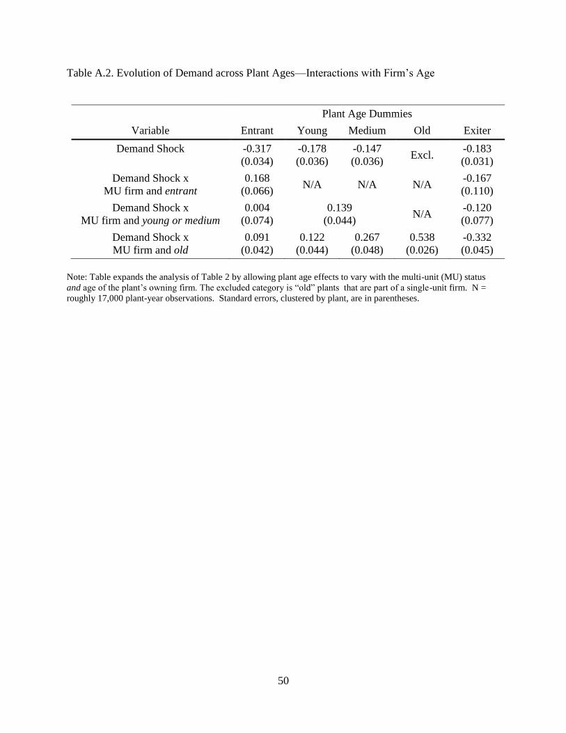
50
Table A.2. Evolution of Demand across Plant Ages—Interactions with Firm’s Age
Variable
Plant Age Dummies
Entrant Young Medium Old Exiter
Demand Shock
-0.317
(0.034)
-0.178
(0.036)
-0.147
(0.036) Excl.
-0.183
(0.031)
Demand Shock x
MU firm and entrant
0.168
(0.066) N/A N/A N/A
-0.167
(0.110)
Demand Shock x
MU firm and young or medium
0.004
(0.074)
0.139
(0.044) N/A
-0.120
(0.077)
Demand Shock x
MU firm and old
0.091
(0.042)
0.122
(0.044)
0.267
(0.048)
0.538
(0.026)
-0.332
(0.045)
Note: Table expands the analysis of Table 2 by allowing plant age effects to vary with the multi-unit (MU) status
and age of the plant’s owning firm. The excluded category is “old” plants that are part of a single-unit firm. N =
roughly 17,000 plant-year observations. Standard errors, clustered by plant, are in parentheses.

51
Table A.3 Contribution of Owning Firm in Same Industry or Geography: Local Product Plants
Parameter Same
Industry
Same
Geography
0.836
(0.014)
0.854
(0.014)
-
-2.203
(0.095)
-2.096
(0.078)
Young dummy
-0.102
(0.038)
-0.145
(0.042)
Medium age dummy
-0.003
(0.025)
-0.031
(0.027)
0.029
(0.053)
0.217
(0.088)
0.714
(0.028)
0.783
(0.031)
Competitor’s Price 0.546
(0.080)
0.474
(0.077)
1
0.997
(0.026)
0.938
(0.033)
2
0.076
(0.116)
0.185
(0.051)
3
0.210
(0.149)
0.335
(0.092)
Selection Correction, Demand Equation
-0.047
(0.022)
-0.034
(0.019)
Selection Correction, Euler Equation
0.022
(0.006)
0.021
(0.006)
Note: Both columns report results for the joint estimation of demand and Euler equations using plant-year
observations for local products. The only difference in specifications is the inclusion of a term in initializing 𝑍0
reflecting the ratio of firm’s parent/sibling capital in the year of entry in the same industry (column 1) or same
geography (column 2) to the overall firm’s parent/sibling capital. 3 refers to the elasticity of initial demand to ratio
of firm’s K in same industry or geography to plant’s K. See text of the appendix for details.
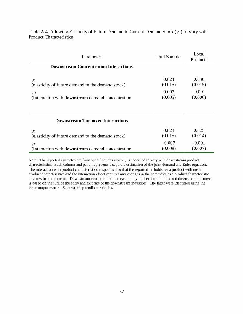
52
Table A.4. Allowing Elasticity of Future Demand to Current Demand Stock ( ) to Vary with
Product Characteristics
Parameter Full Sample Local
Products
Downstream Concentration Interactions
0
(elasticity of future demand to the demand stock)
0.824
(0.015)
0.830
(0.015)
H
(Interaction with downstream demand concentration
0.007
(0.005)
-0.001
(0.006)
Downstream Turnover Interactions
0
(elasticity of future demand to the demand stock)
0.823
(0.015)
0.825
(0.014)
T
(Interaction with downstream demand concentration
-0.007
(0.008)
-0.001
(0.007)
Note: The reported estimates are from specifications where is specified to vary with downstream product
characteristics. Each column and panel represents a separate estimation of the joint demand and Euler equation.
The interaction with product characteristics is specified so that the reported holds for a product with mean
product characteristics and the interaction effect captures any changes in the parameter as a product characteristic
deviates from the mean. Downstream concentration is measured by the herfindahl index and downstream turnover
is based on the sum of the entry and exit rate of the downstream industries. The latter were identified using the
input-output matrix. See text of appendix for details.
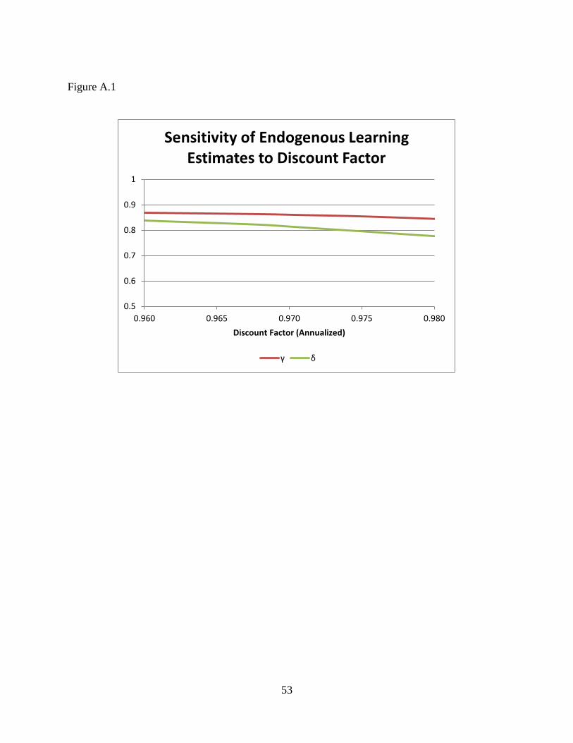
53
Figure A.1
0.5
0.6
0.7
0.8
0.9
1
0.960 0.965 0.970 0.975 0.980
Discount Factor (Annualized)
Sensitivity of Endogenous Learning Estimates to Discount Factor
γ δ