The Snuffle Problem

Denev

for the Numerical Simulation

of a Microreactor

July 2007

The following problem definition is a copy of the Internal Report “A test case formicroreactor flows - a two-dimensional jet in crossflow with chemical reaction” by Car-los J. Falconi, Jordan A. Denev, Jochen Frohlich and Henning Bockhorn that is availableat http://www.ict.uni-karlsruhe.de/index.pl/themen/dns/index.html: “2d test casefor microreactor flows. Internal report. 2007”.

A test case for microreactor flows - a two-dimensional jet in

crossflow with chemical reaction

- Internal Report -

Carlos J. Falconi, Jordan A. Denev, Jochen Frohlich, Henning BockhornInstitute for Technical Chemistry und Polymer Chemistry

University of Karlsruhe (TH)Kaiserstraße 12, 76128 Karlsruhe, Germany

www.ict.uni-karlsruhe.de

December 15, 2006; revised: July 20, 2007

1 Introduction

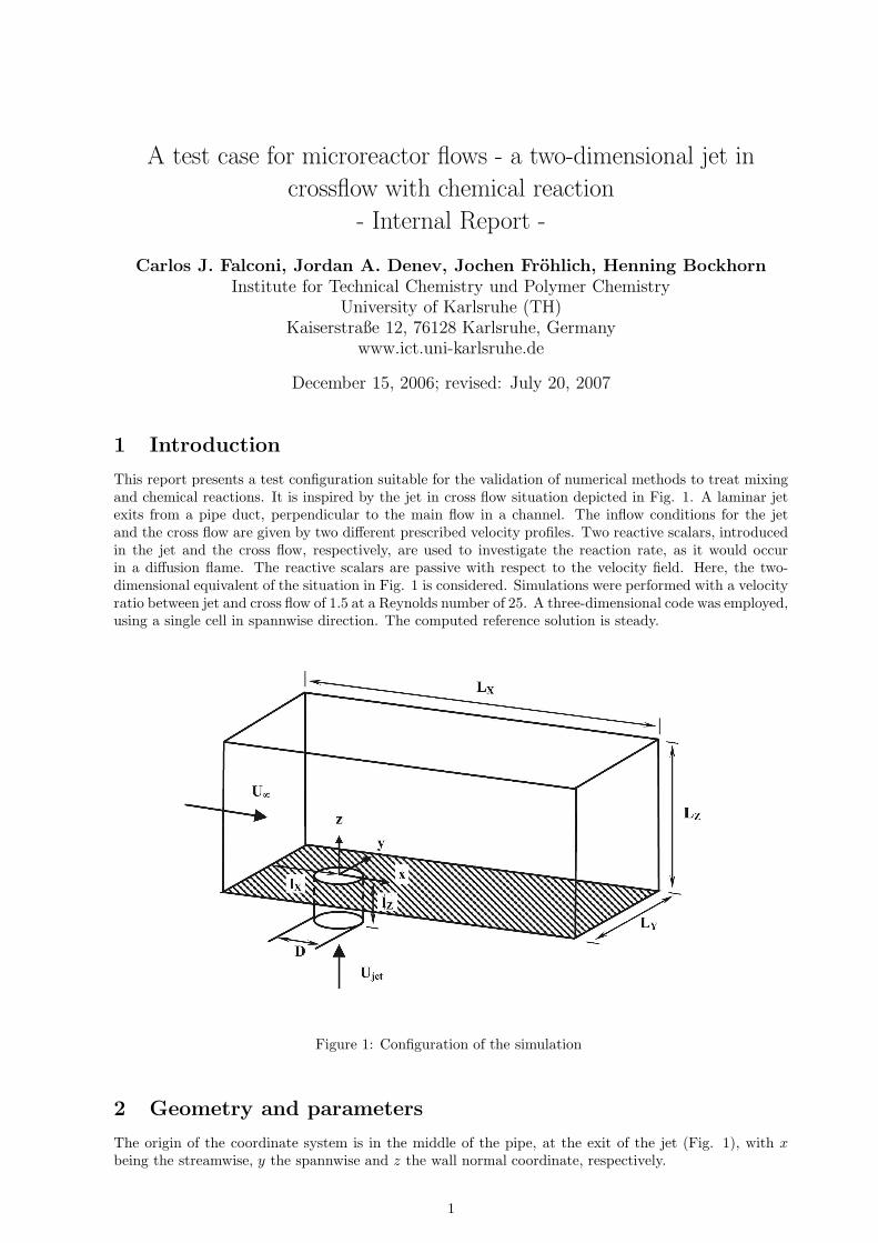
This report presents a test configuration suitable for the validation of numerical methods to treat mixingand chemical reactions. It is inspired by the jet in cross flow situation depicted in Fig. 1. A laminar jetexits from a pipe duct, perpendicular to the main flow in a channel. The inflow conditions for the jetand the cross flow are given by two different prescribed velocity profiles. Two reactive scalars, introducedin the jet and the cross flow, respectively, are used to investigate the reaction rate, as it would occurin a diffusion flame. The reactive scalars are passive with respect to the velocity field. Here, the two-dimensional equivalent of the situation in Fig. 1 is considered. Simulations were performed with a velocityratio between jet and cross flow of 1.5 at a Reynolds number of 25. A three-dimensional code was employed,using a single cell in spannwise direction. The computed reference solution is steady.

Figure 1: Configuration of the simulation

2 Geometry and parameters

The origin of the coordinate system is in the middle of the pipe, at the exit of the jet (Fig. 1), with xbeing the streamwise, y the spannwise and z the wall normal coordinate, respectively.

1

The geometry is the two-dimensional equivalent of the one depicted in Fig. 1. It is defined by theparameters

D = 1; Lx = 16; Ly = 0.1∗; Lz = 4; lx = 3.5; lz = 2*(cf. Introduction)

3 Basic equations

For generality, the equations are provided in their three-dimensional version here. Spacial coordinates arex in streamwise, y in spanwise, and z in wall-normal direction, with velocity components (u, v, w); p ispressure, ρ density, µ dynamic viscosity, and ν = µ/ρ the kinematic viscosity. Nondimensional equationsare used with reference length being the diameter D of the jet and reference velocity the velocity U∞ ofthe cross flow. Density is assumed constant (i.e. equal in jet and crossflow), buonyancy hence does notoccur. Mass fractions are denoted by Y , reaction rates by ω, and diffusion coefficients by Γ. The equationsthen read

• Continuity equation:

∂u

∂x+∂v

∂y+∂w

∂z= 0 (1)

• Momentum equations:

ρ (∂u

∂t+ u

∂u

∂x+ v

∂u

∂y+ w

∂u

∂z) = − ∂p

∂x+ µ (

∂2u

∂x2+∂2u

∂y2+∂2u

∂z2) (2)

ρ (∂v

∂t+ u

∂v

∂x+ v

∂v

∂y+ w

∂v

∂z) = −∂p

∂y+ µ (

∂2v

∂x2+∂2v

∂y2+∂2v

∂z2) (3)

ρ (∂w

∂t+ u

∂w

∂x+ v

∂w

∂y+ w

∂w

∂z) = −∂p

∂z+ µ (

∂2w

∂x2+∂2w

∂y2+∂2w

∂z2) (4)

• Chemistry

Two reactive scalars are introduces, scalar A with the jet, scalar B with the cross flow reacting tothe product Q.

A+BDa−→ Q (5)

• Transport of scalar quantities

ρ (∂YA∂t

+ u∂YA∂x

+ v∂YA∂y

+ w∂YA∂z

) = ρ ΓA (∂2YA∂x2

+∂2YA∂y2

+∂2YA∂z2

) + ωA (6)

ωA = −Da YA YB

ρ (∂YB∂t

+ u∂YB∂x

+ v∂YB∂y

+ w∂YB∂z

) = ρ ΓB (∂2YB∂x2

+∂2YB∂y2

+∂2YB∂z2

) + ωB (7)

ωB = ωA

• Reaction product Q:

YQ = 1− YA − YB (8)

4 Characteristic numbers

• Velocities and Reynolds number:

Reference velocity is the crossflow velocity far from the wall U∞. The jet velocity Ujet is the mean

velocity in the pipe. The ratio of both is R =UjetU∞

. The Reynolds number is defined as Re∞ = U∞Dν .

The present case is defined with R = 1.5 and Re = 25.

2

• Scalar properties:

The following physical properties are chosen ρ = const., ΓA = ΓB = ΓQ = Γ, Sc = 1, Da = 1.

• Dimensionless form of equations

If the above notation of the transport equations is used the natural choice of reference quantitiesleads to posing ρ = 1, ν = 1/Re, Γ = 1/Re.

5 Boundary conditions

Using the above reference quantities the following boundary conditions are specified in non-dimensionalform.

• Cross flow: entry of the main channel

u = 1− e−5ζ , ζ = min ( z, Lz − z ) (9)

w = 0

YA = 0

YB = 1

YQ = 0

• Entry of pipe

u = 0

w = R 2 ( 1− (2r)2 ), r = x

YA = 1

YB = 0

YQ = 0

• Exit of main channel: Homogeneous Neumann condition, i.e. gradient equal to zero for all quantities.

• Top and and bottom wall: no slip for the velocities and vanishing wall-normal gradient for thescalars.

x

z

-2 0 2 4 6 8 10 12-2

-1

0

1

2

3

4

5 | V |3.002.752.492.241.981.731.471.220.960.710.450.20

Figure 2: Streamlines and velocity magnitude |V |.

6 Results:

A reference computation was done, employing the code LESOCC2 previously used for the turbulentthree-dimensional configuration [1]. It solves the three-dimensional incompressible unsteady Navier-Stokesequations using a central second-order finite volume discrization for all derivatives in space and multi-block structure grid treatment for complex geometry. The time scheme is a second order three-stageRunge-Kutta scheme.

The domain is discretized with 20800 cells. In the pipe 55 cells in x-direction have been used withuniform spacing, while in z-direction the grid is clustered near the outlet of the pipe, using 44 cells with

3

x

z

-2 0 2 4 6 8 10 12-2

-1

0

1

2

3

4

5

YQ0.800.600.400.20

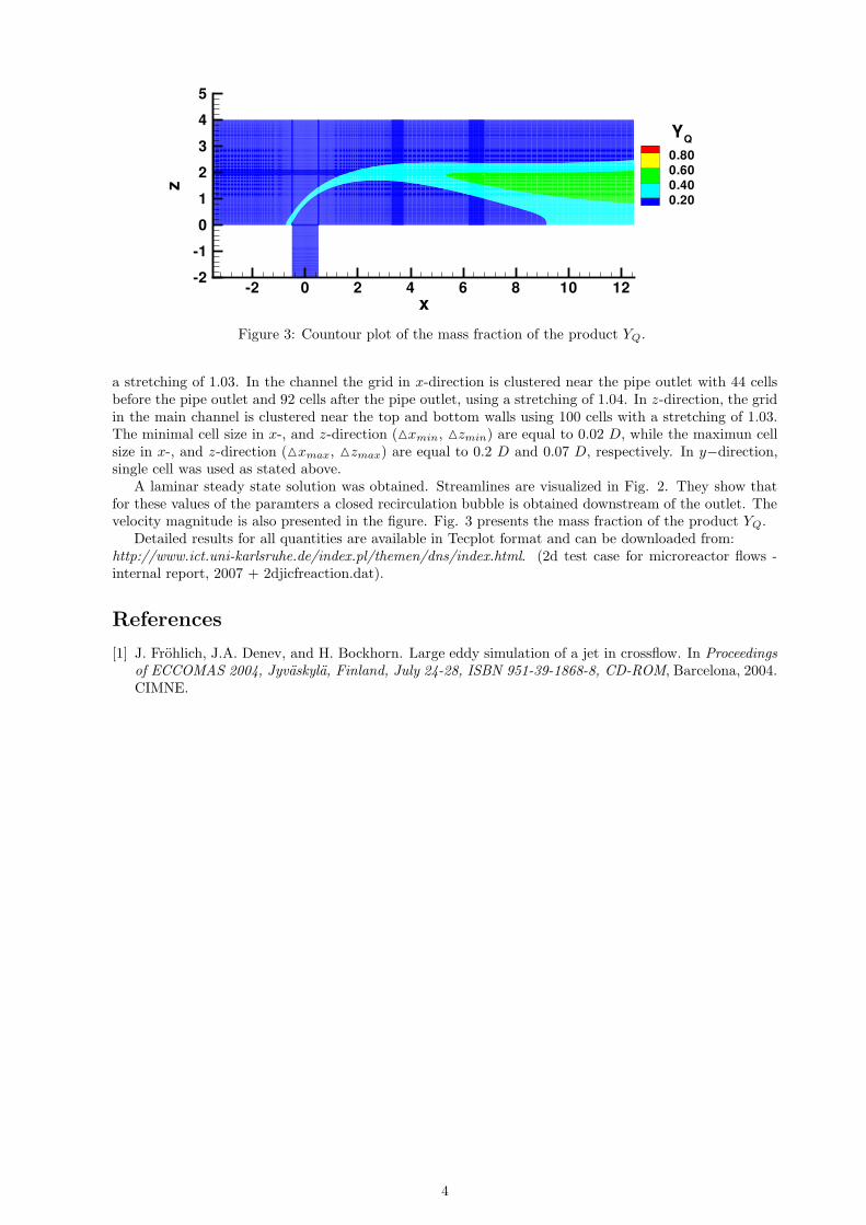
Figure 3: Countour plot of the mass fraction of the product YQ.

a stretching of 1.03. In the channel the grid in x-direction is clustered near the pipe outlet with 44 cellsbefore the pipe outlet and 92 cells after the pipe outlet, using a stretching of 1.04. In z-direction, the gridin the main channel is clustered near the top and bottom walls using 100 cells with a stretching of 1.03.The minimal cell size in x-, and z-direction (Mxmin, Mzmin) are equal to 0.02 D, while the maximun cellsize in x-, and z-direction (Mxmax, Mzmax) are equal to 0.2 D and 0.07 D, respectively. In y−direction,single cell was used as stated above.

A laminar steady state solution was obtained. Streamlines are visualized in Fig. 2. They show thatfor these values of the paramters a closed recirculation bubble is obtained downstream of the outlet. Thevelocity magnitude is also presented in the figure. Fig. 3 presents the mass fraction of the product YQ.

Detailed results for all quantities are available in Tecplot format and can be downloaded from:http://www.ict.uni-karlsruhe.de/index.pl/themen/dns/index.html. (2d test case for microreactor flows -internal report, 2007 + 2djicfreaction.dat).

References

[1] J. Frohlich, J.A. Denev, and H. Bockhorn. Large eddy simulation of a jet in crossflow. In Proceedingsof ECCOMAS 2004, Jyvaskyla, Finland, July 24-28, ISBN 951-39-1868-8, CD-ROM, Barcelona, 2004.CIMNE.

4

Results of the Snuffle Problem Denevby the FDEM Program

Torsten Adolph and Willi Schonauer

Forschungszentrum Karlsruhe, Institute for Scientific Computing,Hermann-von-Helmholtz-Platz 1, 76344 Eggenstein-Leopoldshafen, Germany{torsten.adolph,willi.schoenauer}@iwr.fzk.de

http://www.fzk.de/iwr

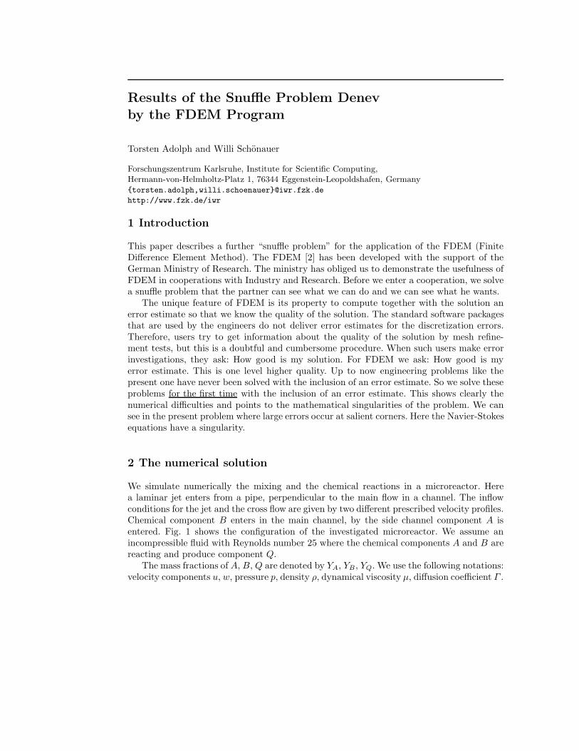
1 Introduction

This paper describes a further “snuffle problem” for the application of the FDEM (FiniteDifference Element Method). The FDEM [2] has been developed with the support of theGerman Ministry of Research. The ministry has obliged us to demonstrate the usefulness ofFDEM in cooperations with Industry and Research. Before we enter a cooperation, we solvea snuffle problem that the partner can see what we can do and we can see what he wants.

The unique feature of FDEM is its property to compute together with the solution anerror estimate so that we know the quality of the solution. The standard software packagesthat are used by the engineers do not deliver error estimates for the discretization errors.Therefore, users try to get information about the quality of the solution by mesh refine-ment tests, but this is a doubtful and cumbersome procedure. When such users make errorinvestigations, they ask: How good is my solution. For FDEM we ask: How good is myerror estimate. This is one level higher quality. Up to now engineering problems like thepresent one have never been solved with the inclusion of an error estimate. So we solve theseproblems for the first time with the inclusion of an error estimate. This shows clearly thenumerical difficulties and points to the mathematical singularities of the problem. We cansee in the present problem where large errors occur at salient corners. Here the Navier-Stokesequations have a singularity.

2 The numerical solution

We simulate numerically the mixing and the chemical reactions in a microreactor. Herea laminar jet enters from a pipe, perpendicular to the main flow in a channel. The inflowconditions for the jet and the cross flow are given by two different prescribed velocity profiles.Chemical component B enters in the main channel, by the side channel component A isentered. Fig. 1 shows the configuration of the investigated microreactor. We assume anincompressible fluid with Reynolds number 25 where the chemical components A and B arereacting and produce component Q.

The mass fractions of A, B, Q are denoted by YA, YB, YQ. We use the following notations:velocity components u, w, pressure p, density ρ, dynamical viscosity µ, diffusion coefficient Γ .

2 Results of the Snuffle Problem Denev by the FDEM Program

x

z

16

4

2.5

1

2

�

�

�

�

�

�

�

�

1

2 3

4

5

6

7

8

in1

in2

out

Fig. 1. Configuration of the investigated microreactor in 2-D.

As prescribed in the problem definition [1], we use nondimensional equations with ref-erence length being the diameter D of the jet and reference velocity the velocity U∞ of thecross flow. The PDEs given in the problem definition [1] are simplified for the 2-D situation,so it holds the following system of six PDEs for the six variables u, w, p, YA, YB, YQ:

• continuity equation for the mixture

∂u

∂x+

∂w

∂z= 0, (1)

• two momentum equations for the mixture

ρ

(u

∂u

∂x+ w

∂u

∂z

)= − ∂p

∂x+ µ

(∂2u

∂x2+

∂2u

∂z2

), (2)

ρ

(u

∂w

∂x+ w

∂w

∂z

)= −∂p

∂z+ µ

(∂2w

∂x2+

∂2w

∂z2

), (3)

• two continuity equations for the components YA, YB

ρ

(u

∂YA

∂x+ w

∂YA

∂z

)= ρΓA

(∂2YA

∂x2+

∂2YA

∂z2

)− DaYAYB, (4)

ρ

(u

∂YB

∂x+ w

∂YB

∂z

)= ρΓB

(∂2YB

∂x2+

∂2YB

∂z2

)− DaYAYB , (5)

• Dalton’s lawYQ = 1 − YA − YB. (6)

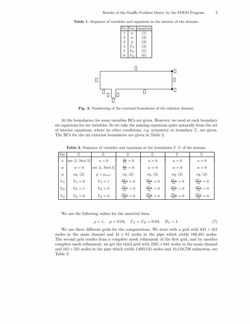
In Table 1 we show which equation is used in which position in the system of PDEs for thenodes in the interior of the domain.

The next problem we want to discuss are the boundary conditions for the six types ofboundaries ① to ⑥ of Fig. 2. In the right corners, we need some BCs from the upper/lowerboundary ④ and some BCs of the right boundary ③, so these corner nodes have to be definedas an additional boundary.

Results of the Snuffle Problem Denev by the FDEM Program 3

Table 1. Sequence of variables and equations in the interior of the domain.

No. Var. equation

1 u (1)2 w (3)3 p (2)4 YA (4)5 YB (5)6 YQ (6)

�

�

①

②

③

④

④④⑤ ⑤

⑥

⑥

Fig. 2. Numbering of the external boundaries of the solution domain.

At the boundaries, for some variables BCs are given. However, we need at each boundarysix equations for six variables. So we take the missing equations quite naturally from the setof interior equations, where no other conditions, e.g. symmetry at boundary ③, are given.The BCs for the six external boundaries are given in Table 2.

Table 2. Sequence of variables and equations at the boundaries ①–⑥ of the domain.

Var. ① ② ③ ④ ⑤ ⑥

u see [1, Sect.5] u = 0 ∂u∂x

= 0 u = 0 u = 0 u = 0

w w = 0 see [1, Sect.5] ∂w∂x

= 0 w = 0 w = 0 w = 0

p eq. (2) p = patm eq. (2) eq. (3) eq. (3) eq. (2)

YA YA = 0 YA = 1 ∂YA∂x

= 0 ∂YA∂y

= 0 ∂YA∂x

= 0 ∂YA∂y

= 0

YB YB = 1 YB = 0 ∂YB∂x

= 0 ∂YB∂y

= 0 ∂YB∂x

= 0 ∂YB∂y

= 0

YQ YQ = 0 YQ = 0∂YQ

∂x= 0

∂YQ

∂y= 0

∂YQ

∂x= 0

∂YQ

∂y= 0

We use the following values for the material data:

ρ = 1, µ = 0.04, ΓA = ΓB = 0.04, Da = 1. (7)

We use three different grids for the computations. We start with a grid with 641 × 161nodes in the main channel and 41 × 81 nodes in the pipe which yields 106,481 nodes.The second grid results from a complete mesh refinement of the first grid, and by anothercomplete mesh refinement, we get the third grid with 2561× 641 nodes in the main channeland 161× 321 nodes in the pipe which yields 1,693,121 nodes and 10,158,726 unknowns, seeTable 3.

4 Results of the Snuffle Problem Denev by the FDEM Program

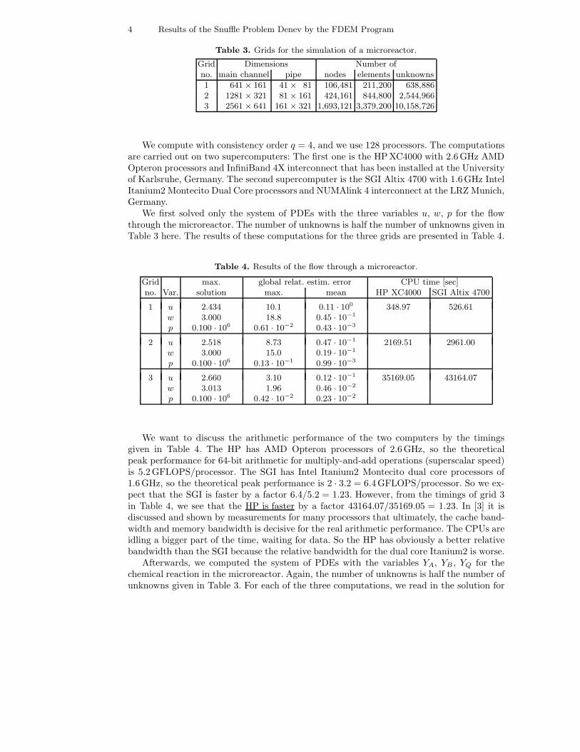
Table 3. Grids for the simulation of a microreactor.

Grid Dimensions Number ofno. main channel pipe nodes elements unknowns

1 641 × 161 41 × 81 106,481 211,200 638,8862 1281 × 321 81 × 161 424,161 844,800 2,544,9663 2561 × 641 161 × 321 1,693,121 3,379,200 10,158,726

We compute with consistency order q = 4, and we use 128 processors. The computationsare carried out on two supercomputers: The first one is the HP XC4000 with 2.6GHz AMDOpteron processors and InfiniBand 4X interconnect that has been installed at the Universityof Karlsruhe, Germany. The second supercomputer is the SGI Altix 4700 with 1.6GHz IntelItanium2 Montecito Dual Core processors and NUMAlink 4 interconnect at the LRZ Munich,Germany.

We first solved only the system of PDEs with the three variables u, w, p for the flowthrough the microreactor. The number of unknowns is half the number of unknowns given inTable 3 here. The results of these computations for the three grids are presented in Table 4.

Table 4. Results of the flow through a microreactor.

Grid max. global relat. estim. error CPU time [sec]no. Var. solution max. mean HP XC4000 SGI Altix 4700

1 u 2.434 10.1 0.11 · 100 348.97 526.61w 3.000 18.8 0.45 · 10−1

p 0.100 · 106 0.61 · 10−2 0.43 · 10−3

2 u 2.518 8.73 0.47 · 10−1 2169.51 2961.00w 3.000 15.0 0.19 · 10−1

p 0.100 · 106 0.13 · 10−1 0.99 · 10−3

3 u 2.660 3.10 0.12 · 10−1 35169.05 43164.07w 3.013 1.96 0.46 · 10−2

p 0.100 · 106 0.42 · 10−2 0.23 · 10−2

We want to discuss the arithmetic performance of the two computers by the timingsgiven in Table 4. The HP has AMD Opteron processors of 2.6GHz, so the theoreticalpeak performance for 64-bit arithmetic for multiply-and-add operations (superscalar speed)is 5.2GFLOPS/processor. The SGI has Intel Itanium2 Montecito dual core processors of1.6GHz, so the theoretical peak performance is 2 · 3.2 = 6.4GFLOPS/processor. So we ex-pect that the SGI is faster by a factor 6.4/5.2 = 1.23. However, from the timings of grid 3in Table 4, we see that the HP is faster by a factor 43164.07/35169.05 = 1.23. In [3] it isdiscussed and shown by measurements for many processors that ultimately, the cache band-width and memory bandwidth is decisive for the real arithmetic performance. The CPUs areidling a bigger part of the time, waiting for data. So the HP has obviously a better relativebandwidth than the SGI because the relative bandwidth for the dual core Itanium2 is worse.

Afterwards, we computed the system of PDEs with the variables YA, YB , YQ for thechemical reaction in the microreactor. Again, the number of unknowns is half the number ofunknowns given in Table 3. For each of the three computations, we read in the solution for

Results of the Snuffle Problem Denev by the FDEM Program 5

Table 5. Results of the chemical reaction in a microreactor.

Grid max. global relat. estim. error CPU time [sec]no. Var. solution max. mean HP XC 4000 SGI Altix 4700

1 YA 1.444 4.27 0.68 · 10−2 145.13 219.70YB 1.000 4.07 0.70 · 10−2

YQ 0.609 3.93 0.12 · 10−1

2 YA 1.061 2.13 0.14 · 10−2 1267.80 1708.29YB 1.000 1.39 0.71 · 10−3

YQ 0.602 1.45 0.19 · 10−2

3 YA 1.000 1.15 0.14 · 10−2 16178.16 20362.58YB 1.000 0.71 0.85 · 10−3

YQ 0.597 0.75 0.19 · 10−2

u, w that we have just computed from the u, w, p-system. This means that the flow velocitiesu and w are constant for the computation of the chemical components. The results of thesecomputations for the three grids are presented in Table 5.

Table 6. Results of the simulation of a microreactor.

Grid max. global relat. estim. error CPU time [sec]no. Var. solution max. mean HP XC4000 SGI Altix 4700

1 u 2.434 10.1 0.11 · 100 189.10 264.03w 3.000 18.8 0.45 · 10−1

p 0.100 · 106 0.61 · 10−2 0.43 · 10−3

YA 1.444 5.96 0.61 · 10−1

YB 1.000 5.93 0.97 · 10−1

YQ 0.609 4.37 0.12 · 100

2 u 2.518 8.73 0.47 · 10−1 2378.02 2612.45w 3.000 15.0 0.19 · 10−1

p 0.100 · 106 0.13 · 10−1 0.99 · 10−3

YA 1.061 2.25 0.27 · 10−1

YB 1.000 1.46 0.37 · 10−1

YQ 0.602 1.54 0.42 · 10−1

3 u 2.660 3.10 0.12 · 10−1 40450.32 49718.47w 3.013 1.96 0.46 · 10−2

p 0.100 · 106 0.42 · 10−2 0.23 · 10−2

YA 1.000 1.23 0.12 · 10−1

YB 1.000 0.78 0.94 · 10−2

YQ 0.597 0.74 0.24 · 10−1

As the system of PDEs for the flow through the microreactor is completely independent(decoupled) from the system of PDEs for the chemical components, it is of no importancefor the solution and for the errors of the velocity components and the pressure whetherwe compute the solution of the two systems with three PDEs each, or the solution of thecomplete system with six PDEs. However, the velocity field affects the chemical components

6 Results of the Snuffle Problem Denev by the FDEM Program

so that we get in fact the same solution if we compute the solution of the system with sixPDEs but the errors change as there enter the errors of the velocity components.

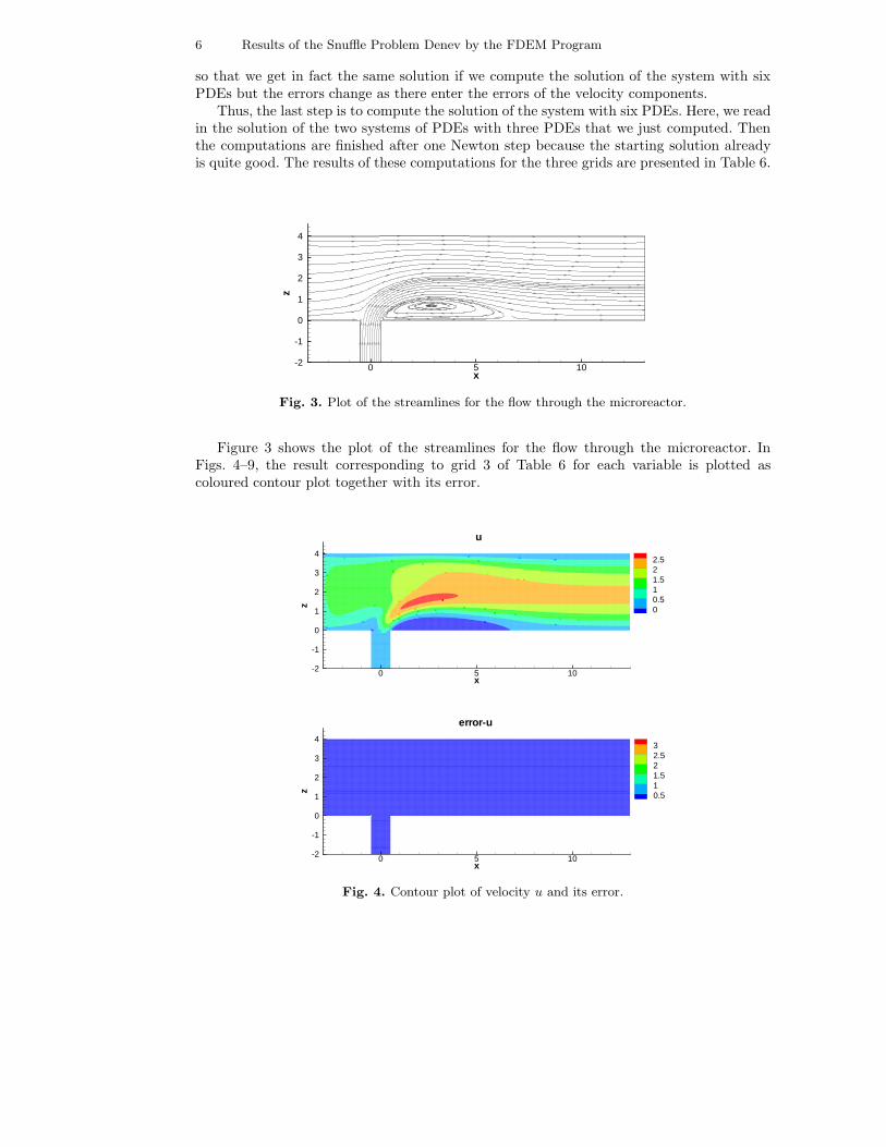
Thus, the last step is to compute the solution of the system with six PDEs. Here, we readin the solution of the two systems of PDEs with three PDEs that we just computed. Thenthe computations are finished after one Newton step because the starting solution alreadyis quite good. The results of these computations for the three grids are presented in Table 6.

x

z

0 5 10-2

-1

0

1

2

3

4

Fig. 3. Plot of the streamlines for the flow through the microreactor.

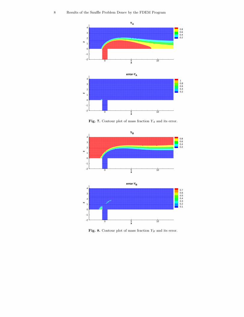
Figure 3 shows the plot of the streamlines for the flow through the microreactor. InFigs. 4–9, the result corresponding to grid 3 of Table 6 for each variable is plotted ascoloured contour plot together with its error.

x

z

0 5 10-2

-1

0

1

2

3

42.521.510.50

u

x

z

0 5 10-2

-1

0

1

2

3

432.521.510.5

error-u

Fig. 4. Contour plot of velocity u and its error.

Results of the Snuffle Problem Denev by the FDEM Program 7

x

z

0 5 10-2

-1

0

1

2

3

42.521.510.50

w

x

z

0 5 10-2

-1

0

1

2

3

41.510.5

error-w

Fig. 5. Contour plot of velocity w and its error.

x

z

0 5 10-2

-1

0

1

2

3

4100040100030100020100010100000

p

x

z

0 5 10-2

-1

0

1

2

3

40.0040.0030.0020.001

error-p

Fig. 6. Contour plot of pressure p and its error.

8 Results of the Snuffle Problem Denev by the FDEM Program

x

z

0 5 10-2

-1

0

1

2

3

40.80.60.40.2

YA

x

z

0 5 10-2

-1

0

1

2

3

410.80.60.40.2

error-YA

Fig. 7. Contour plot of mass fraction YA and its error.

x

z

0 5 10-2

-1

0

1

2

3

40.80.60.40.2

YB

x

z

0 5 10-2

-1

0

1

2

3

40.70.60.50.40.30.20.1

error-YB

Fig. 8. Contour plot of mass fraction YB and its error.

Results of the Snuffle Problem Denev by the FDEM Program 9

x

z

0 5 10-2

-1

0

1

2

3

40.50.40.30.20.1

YQ

x

z

0 5 10-2

-1

0

1

2

3

40.70.60.50.40.30.20.1

error-YQ

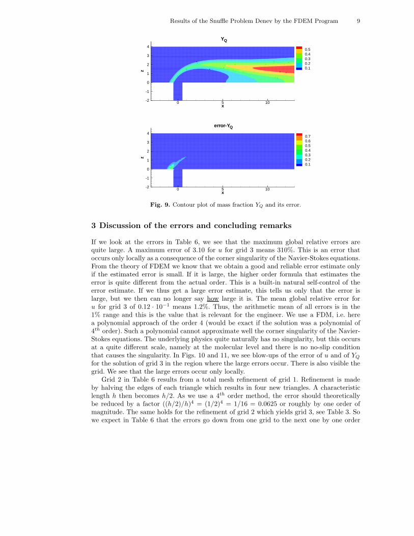
Fig. 9. Contour plot of mass fraction YQ and its error.

3 Discussion of the errors and concluding remarks

If we look at the errors in Table 6, we see that the maximum global relative errors arequite large. A maximum error of 3.10 for u for grid 3 means 310%. This is an error thatoccurs only locally as a consequence of the corner singularity of the Navier-Stokes equations.From the theory of FDEM we know that we obtain a good and reliable error estimate onlyif the estimated error is small. If it is large, the higher order formula that estimates theerror is quite different from the actual order. This is a built-in natural self-control of theerror estimate. If we thus get a large error estimate, this tells us only that the error islarge, but we then can no longer say how large it is. The mean global relative error foru for grid 3 of 0.12 · 10−1 means 1.2%. Thus, the arithmetic mean of all errors is in the1% range and this is the value that is relevant for the engineer. We use a FDM, i.e. herea polynomial approach of the order 4 (would be exact if the solution was a polynomial of4th order). Such a polynomial cannot approximate well the corner singularity of the Navier-Stokes equations. The underlying physics quite naturally has no singularity, but this occursat a quite different scale, namely at the molecular level and there is no no-slip conditionthat causes the singularity. In Figs. 10 and 11, we see blow-ups of the error of u and of YQ

for the solution of grid 3 in the region where the large errors occur. There is also visible thegrid. We see that the large errors occur only locally.

Grid 2 in Table 6 results from a total mesh refinement of grid 1. Refinement is madeby halving the edges of each triangle which results in four new triangles. A characteristiclength h then becomes h/2. As we use a 4th order method, the error should theoreticallybe reduced by a factor ((h/2)/h)4 = (1/2)4 = 1/16 = 0.0625 or roughly by one order ofmagnitude. The same holds for the refinement of grid 2 which yields grid 3, see Table 3. Sowe expect in Table 6 that the errors go down from one grid to the next one by one order

10 Results of the Snuffle Problem Denev by the FDEM Program

x

z

-0.55 -0.5 -0.45 -0.4-0.04

-0.03

-0.02

-0.01

0

0.01

0.02

0.03 32.521.510.5

Fig. 10. Blow-up of the contour plot of the error of velocity u.

x

z

-0.55 -0.5 -0.45 -0.4-0.04

-0.03

-0.02

-0.01

0

0.01

0.02

0.03 0.70.60.50.40.30.20.1

Fig. 11. Blow-up of the contour plot of the error of mass fraction YQ.

of magnitude. However, for the most interesting component of this calculation, the reactionproduct mass fraction YQ, we see in Table 6 a reduction of the maximum error by a factor0.35 from grid 1 to 2 and by 0.48 from grid 2 to 3. For the mean errors hold factors 0.35and 0.57, respectively.

Why is this error reduction so far away from the theoretically expected value? The reasonis the above mentioned singularity of the Navier-Stokes equations at salient corners. Thefiner the grid, the better the singularity is detected, but the theoretically expected reductionof the error does not occur because the polynomial approach of the FDM cannot resolve asingularity. We must live with this fact. People that use standard software packages are notaware of that.

In conclusion we can say that the numerical solution of PDEs that includes an errorestimate gives a quite new insight in the numerical result. Because of the singularity of theNavier-Stokes equations a total mesh refinement reduces the error only linearly, roughly by afactor of 0.5 instead of the expected reduction by an order of magnitude. How the singularityof the pure flow equations then affects the accuracy of the chemical components, e.g. of YQ,can only be seen from the error estimate of the numerical result.

References

1. Falconi, C.J., Denev, J.A., Frohlich, J., Bockhorn, H., A test case for microreactor flows - atwo-dimensional jet in crossflow with chemical reaction, Internal Report, available athttp://www.ict.uni-karlsruhe.de/index.pl/themen/dns/index.html: “2d test case for mi-croreactor flows. Internal report. 2007”. This paper is included above in this file.

Results of the Snuffle Problem Denev by the FDEM Program 11

2. Schonauer, W., Adolph, T., FDEM: The Evolution and Application of the Finite DifferenceElement Method (FDEM) Program Package for the Solution of Partial Differential Equations,Abschlussbericht des Verbundprojekts FDEM, Universitat Karlsruhe, 2005, available athttp://www.rz.uni-karlsruhe.de/rz/docs/FDEM/Literatur/fdem.pdf

3. Schonauer, W., Scientific Supercomputing, Selfedition Willi Schonauer, 2000, E-Mail:schoenauer@rz.uni-karlsruhe.de