The Social Discount Rate under

Intertemporal Risk Aversion and Ambiguity

First version: December 2007 – this version: August 2008

Christian P. TRAEGER

Department of Agricultural & Resource Economics, UC Berkeley

Abstract: Following the Stern review of climate change the numerical choiceof the social discount rate has been identified as one of the most crucial de-terminants of optimal policy recommendations for greenhouse gas mitigationpolicies. In this paper I point out two closely related contributions to thesocial discount rate in an uncertain world that have been overlooked in thedebate. First, the standard model that has been employed in the debatecontains an implicit assumption of (intertemporal) risk neutrality, stemmingfrom the assumption that Arrow Pratt risk aversion is equivalent to theaversion to intertemporal consumption fluctuations. Second, the recent de-cision theoretic literature has developed various models that generalize thedescription of uncertainty in order to explain observed differences in the at-titude with respect to risk versus ambiguous uncertainty. I show how thesetwo extensions of the standard model modify the (certainty equivalent) socialdiscount rate and point out that there is reason to believe that the additionalcontribution from intertemporal risk aversion is significantly larger than theterm capturing risk in the social discount rate based on the standard model.

JEL Codes: D61, D81, D90, H43, Q00, Q54

Keywords: ambiguity, discounting, expected utility, intertemporal substi-tutability, intertemporal risk aversion, recursive utility, risk aversion, socialdiscount rate, uncertainty

Correspondence:

Department of Agricultural & Resource Economics207 Giannini Hall #3310University of CaliforniaBerkeley, CA 94720-3310E-mail: traeger@berkeley.edu

1 Introduction

Stern’s (2007) review of climate change implied a significantly quicker andstronger action for greenhouse gas mitigation than most of the integrated as-sessments previously carried out in the literature. The difference between theresults was mostly attributed to Stern’s (2007) choice of the social discountrate whose ‘correct value’ has been hotly debated with some of the argumentssummarized in Nordhaus (2007), Weitzman (2007b) and Weitzman (2007a),and Dasgupta (2008b). In the classical Ramsey (1928) formulation the so-cial discount rate comprises pure time preference and a term that expressesthe change in marginal consumption appreciation caused by a combination ofgrowth and the propensity to smooth consumption over time. Another contri-bution arises from considering risk and Arrow Pratt risk aversion. Essentially,these are the contributions whose quantifications were so hotly debated.1 Ishow that a further and significant contribution stems from acknowledgingintertemporal risk aversion as well as from acknowledging ambiguity.

Time and uncertainty constitute an essential ingredient to many of themost challenging environmental economic problems. However, in their com-bination the two have been treated rather negligently in the literature. Thediscounted expected utility standard model (which is additive in time anduncertainty) implicitly sets Arrow Pratt risk aversion equal to the aversionto intertemporal consumption flucutations. In two recent working papers Ihave pointed out that this assumption is effectively an assumption of riskneutrality (Traeger 2007e, Traeger 2007c). A precise difference between Ar-row Pratt risk aversion and the (inverse of the) intertemporal elasticity ofsubstitution is itself a measure of risk attitude that I tagged intertemporalrisk attitude. Intertemporal risk aversion can be understood as an aversionto utility gains and losses (as opposed to consumption gains and losses).2

After a presentation of the general model of intertemporal risk aversion, Iderive the corresponding social discount rate in a simple two period settingwith a stochastic growth rate. For this purpose I employ a special case ofthe model that has already been formulated by Epstein & Zin (1989) and

1A different adjustment stems from limited substitutability between goods under un-balanced growth as it can prevail for produced versus environmental goods (Guesnerie2004, Hoel & Sterner 2007, Traeger 2007d, Sterner & Persson 2008).

2This intuition holds for a representation framework where aggregation is additive overtime and nonlinear over uncertainty. Here, the utility function captures the attitude withrespect to time and consumption appreciation under certainty.

1

Weil (1990). Besides some analytical convenience, this generalized isoelasticversion of the model has the advantage that several attempts have been madeto estimate its parameters. In consequence, I can give estimates of the sizeof the derived term in the social discount rate that has been neglected in thedebate.

A different strand of literature developing over the last two decades mod-els uncertainty without assuming the existence of unique probability mea-sures. In axiomatic terms, these models relax the von Neumann & Morgen-stern (1944) (or Savage 1954) axioms. Facing problems of climate change, lostprospects from reduced biodiversity, or ecosystem changes caused by possibleinvasive species it has often been pointed out that uncertainties are likely tobe different from standard notions of risk and that they are not capturedappropriately by applying a unique probability distribution. Here, decisionmakers might not know the probability distribution (objective probabilities),nor trust a single subjective guess (subjective probabilistic belief). I adopta recent model of ambiguity by Klibanoff, Marinacci & Mukerji (2005) andKlibanoff, Marinacci & Mukerji (2009) that distinguishes between risk andmore general uncertainty by employing first and second order probabilities.A convenience of this model is its resemblance to the standard Bayesianmodel. However, the key difference is that Klibanoff et. al’s model capturesdifferent degrees of aversion for risk and ambiguous uncertainty. I derive thecontribution of ambiguity aversion to the social discount rate in a simple twoperiod version of the model. Section 2 lays out the models of intertemporalrisk averse decision making and decision making under ambiguity. Section 3derives the social discount rates under intertemporal risk aversion and underambiguity. Section 4 concludes.

2 Intertemporal Models of Risk Attitude &

Ambiguity

It is well known that the intertemporally additive expected utility frameworkfor modeling preferences implicitly assumes that a decision maker’s aversionto risk coincides with his aversion to intertemporal fluctuations. Epstein &Zin (1989) and Weil (1990) derive an alternative setting in which these two apriori quite different characteristics of preference can be disentangled. Thissection presents a slightly more general framework framework introducing

2

the concept of intertemporal risk aversion (Traeger 2007e, Traeger 2007c).The generalization permits a simple and intuitive derivation of the modeland an enlightening axiomatic characterization of the type of risk aversionit can capture as opposed to the standard model. Subsequently, the sectionsummarizes a recent intertemporal ambiguity model by Klibanoff, Marinacci& Mukerji (2006) that captures uncertainty in a more general way than bymeans of unique probability distributions.

2.1 An Intertemporal Model of Risk Attitude

The simplest framework to convey the message of this paper is the ‘certain× uncertain’ setting, two periods with uncertainty only in the future period.I denote first period consumption by x1 ∈ X and uncertain second periodconsumption is represented by a probability measure p over X.3 I will referto the ‘standard model’ as the modeling framework where a decision makerevaluates utility separately for every period and for every state of the worldand then sums it over states and over time

U s(x1, p) = u(x1) + βEpu(x2) , (1)

where β is the utility discount factor representing pure time preference. Thecurvature of u captures the decision maker’s aversion to consumption fluc-tuations. Because the same utility function is used to aggregate over timeand over risk, the decision maker’s aversion to (certain) intertemporal fluc-tuations is the same as his aversion to risk fluctuations corresponding todifferent states of the world.

A priori, however, risk aversion and the propensity to smooth consump-tion over time are two distinct concepts. The notion that in an atemporalsetting risky scenarios can be evaluated in the form

U2(p) = EpuvNM(x) (2)

is based on the von Neumann & Morgenstern (1944) axioms. Here, thecurvature of uvNM captures risk aversion. For a single commodity setting, theArrow-Pratt measure of relative risk aversion RRA(x) = −u′′(x)

u′(x)x attaches

3Formally, let X be a compact metric space and P be the space of Borel probabilitymeasures on X.

3

a numeric value to curvature and risk aversion. A similar set of axioms4

provides additive separability of preference representations evaluating certainconsumption paths. Adding stationarity to the evaluation makes the utilityfunctions in the different periods coincide up to a discount factor β

U1(x1, x2) = uint(x1) + βuint(x2) (3)

In equation (3) the concavity of the utility function uint describes aversionto intertemporal consumption volatility. In a one commodity setting5 thisaversion to intertemporal volatility can be measured by means of the con-

sumption elasticity of marginal utility η = −uint′′(x)

uint′(x)x. The consumption

elasticity of marginal utility is the inverse of the intertemporal elasticity ofsubstitution. Note that the measure η exactly corresponds to the ArrowPratt measure of relative risk aversion, only in the context of periods ratherthan risk states. Instead of calling η an aversion measure to intertemporalvolatility, it can also be characterized as a measure for a decision maker’spropensity to smooth consumption over time.

The conceptual difference between the utility functions uvNM and uint

was first disentangled by Selden (1978) for the ‘certain × uncertain’ settingadopted here. Epstein & Zin (1989) use a one commodity isoelastic versionof Kreps & Porteus’s (1978) to extend this idea to an infinite time hori-zon. Such an isoelastic extension requires a recursive evaluation in order topreserve time consistency. In Traeger (2007e) I extend this reasoning to amulticommodity setting with more general functional forms, derived fromcombining the von Neumann-Morgenstern axioms with the assumption thatcertain consumption paths can be evaluated in the additively separable form(3). For the ‘certain × uncertain’ setting the derivation of the general modelis particularly simple. As the derivation gives a good intuition of the modeland the concepts used later in this paper I give a brief sketch. Let equation

4See Wakker (1988), Koopmans (1960), Krantz, Luce, Suppes & Tversky (1971), Jaffray(1974a), Jaffray (1974b), Radner (1982), and Fishburn (1992) for various axiomatizationsof additive separability over time. Other than the von Neumann & Morgenstern (1944)axioms, these axioms allow for period specific utility functions (which would correspondto a state dependent utility model in the risk setting).

5Kihlstrom & Mirman (1974) generalized the one commodity measure by Arrow Prattto a multi-commodity setting. Here risk aversion becomes good-specific and corresponds tothe concavity of the utility function along a variation of the particular commodity keepingthe others constant. The same concept of a multi-dimensional measure could be appliedto intertemporal substitutability.

4

(3) represent preferences over certain (two period) consumption paths. Letequation (2) represent preferences over second period lotteries. Define x

p2 as

the second period certainty equivalent to the lottery p by requiring

U2(xp2) = uvNM(xp

2)!= U2(p) = Epu

vNM(x) (4)

⇒ xp2 = uvNM−1 [

EpuvNM(x)

]

.

Now use the certainty equivalent to extend the evaluation functional in equa-tion (3) to a setting of uncertainty by defining

U(x1, p) = U2(x1, xp2) = uint(x1) + βuint

(

uvNM−1 [

EpuvNM(x)

]

)

.

Taking the inverse of uvNM assumes a one dimensional setting. In general, itholds that uvNM is always a strictly monotonic transformation of uint (Traeger2007e).6 Thus, defining f by uvNM = f ◦ uint, I can transform the equality(4) into

f ◦ uint(xp2)

!= Epf ◦ uint(x)

⇔ uint(xp2) = f−1

[

Epf ◦ uint(x)]

and obtain in combination with equation (3) and the definition u ≡ uint therepresentation

U(x1, p) = u(x1) + βf−1 [Epf ◦ u(x)] (5)

for the multi-commodity framework. In general, preferences represented byequation (5) cannot be represented by an evaluation function of the formU s(x1, p) = u1(x1) + Epu2(x) (equation 1).

The definition uvNM = f ◦ uint points out that f is a measure for thedifference between aversion to intertemporal fluctuations (as characterizedby uint in a one-commodity setting) and aversion to risk in the Arrow Prattsense (as characterized by uvNM in a one-commodity setting). For example,f concave is equivalent to uvNM being a concave transformation of uint, which

6In the above setting simply observe that both U1(x1, x2) and U2(x2) = uvNM(x2)for some fixed x1 have to represent the same preferences over X (assuming time con-sistency). Therefore the two different representations have to coincide up to an ordinaltransformation.

5

is a definition of uvNM being more concave than uint (Hardy, Littlewood &Polya 1964). Thus, a concave function f gains an interpretation of repre-senting a decision maker who is more Arrow Pratt risk averse than he isaverse to intertemporal consumption fluctuations. It is insightful to give anaxiomatic characterization of f that characterizes the function in a generalmulticommodity setting and on basis of consumption decisions rather thanutility comparisons.

2.2 Characterizing Intertemporal Risk Attitude

This section gives an axiomatic characterization of the type of uncertaintythat can only be captured in the model of equation (5) and not in the stan-dard model. It turns out that the term reducing the social discount rateis proportional to the quantitative measures of this type of risk aversion.Moreover, I show that functionally this type of risk aversion is captured inthe curvature of the function f . A general stationary and nonstationary ax-iomatic characterizations of f (respectively time dependent series ft,t∈1,...,T )can be found in Traeger (2007c) respectively Traeger (2007e). These axiomsrequire at least two uncertain periods and are slightly more involved. Here,I give a simplified axiom for the ‘certain × uncertain’ setting which conveysthe same intuition as the general axioms, but has to assume the absence ofpure time preference. Let � characterize preferences on X × P correspond-ing to representation (5) with β = 1. Then, I call the corresponding decisionmaker (weakly)7 intertemporal risk averse, if and only if, for all x, x1, x2 ∈ X

(x, x) ∼ (x1, x2) ⇒ (x, x) � (x, 12x1 + 1

2x2) . (6)

The premise in equation (6) states that a decision maker is indifferent be-tween a certain constant consumption path delivering the same outcome x inboth periods and another certain consumption path which delivers outcomex1 in the first and outcome x2 in the second period. For example, x1 can bean inferior outcome with respect to x. Then x2 would be a superior outcomewith respect to x. On the right hand side of equation (6) the decision makerreceives x in the first period, independent of his choice. For the second periodhe has a choice between the certain outcome x or a lottery that returns withequal probability either the superior or the inferior outcome. The decision

7The strong notion would involve the additional requirement (x, x1) 6∼ (x, x2) in thepremise and a strict preference in the implication.

6

maker is called (weakly) intertemporal risk averse if he prefers the certainoutcome x in the second period over the lottery.8 A decision maker is definedas (weakly) intertemporal risk loving if the preference relation � in equation(6) is replaced by �. He is defined to be risk neutral if he is both, intertem-poral risk loving and intertemporal risk averse (relation � in equation (6) isreplaced by ∼). The following proposition relates intertemporal risk aversionto the function f .

Proposition 1: Let preferences over X × P be represented by equation (5)with a continuous function u : X → IR and a strictly increasing andcontinuous function f : U → IR, where U = u(X) and β = 1.a) The corresponding decision maker is (weakly) intertemporal riskaverse [loving], if and only if, the function f is concave [convex].b) The corresponding decision maker is intertemporal risk neutral, ifand only if, there exist a, b ∈ IR such that f(z) = az + b. An intertem-poral risk neutral decision maker maker maximizes intertemporally ad-ditive expected utility (equation 1).9

The proposition shows that intertemporal risk aversion as defined by equa-tion (6) is captured in the curvature of the function f in representation(5). Thus, intertemporal risk aversion can as well be interpreted as riskaversion with respect to utility gains and losses. This interpretation is trueif preferences are represented in the form where the aggregation over time(in every recursion) is additive, as is the case in the representation in thispaper.10 Then, utility expressed by u characterizes how much the decisionmaker likes a particular outcome x or a particular degenerate situation in the

8Let me point out that the lottery on the right hand side of equation (6) will eithermake the decision maker better off or worse off than (x, x), while on the left hand sidethe decision maker knows that if he picks an inferior outcome for some period he certainlyreceives the superior outcome in the other.

Calling preferences satisfying equation (6) intertemporal risk averse is motivated by thefacts that, first, the definition intrinsically builds on intertemporal trade-offs and, second,Normandin & St-Amour (1998, 268) make the point that the conventional Arrow Prattmeasure of risk aversion is an atemporal concept.

9Recasting the proposition for a strictly decreasing continuous function f : U → IRturns concavity in statement a) into convexity [and convexity into concavity]. Replacingthe definition of intertemporal risk aversion by its strict version given in footnote 7 switchesconcavity to strict concavity in the statement.

10See Traeger (2007e) how the same preferences can be represented by making uncer-tainty aggregation linear at the cost of incorporating a nonlinear aggregation over time.

7

future. If the decision maker is intertemporal risk averse, he dislikes takingrisk with respect to gains and losses of such utility. Note that in differenceto the Arrow-Pratt measure of risk aversion, the function f is always onedimensional. Thus, measures of intertemporal risk aversion can be used asa commodity independent risk measure also in a multi-commodity setting.11

Even more interestingly, the measures can be applied to contexts frequentlymet in environmental economics where impacts, e.g. on an ecosystem, donot have a natural cardinal scale (Traeger 2007e). The measure of absoluteintertemporal risk aversion is defined as

AIRA(z) = −f ′′(z)

f ′(z),

and the measure of relative intertemporal risk aversion as

RIRA(z) = −f ′′(z)

f ′(z)|z| .

The measure of absolute intertemporal risk aversion depends on the choiceof unit for utility and the measure RIRA(z) depends on the choice of zeroin the definition of the utility function u. This normalization dependence isthe analog to e.g. the wealth level dependence of the Arrow Pratt measureof relative risk aversion.12 Note that positivity of the measures AIRA andRIRA defined above indicates intertemporal risk aversion independently ofwhether f is increasing and concave of decreasing and convex (see footnote9). In both cases −f ′′

f ′is positive. Measuring utility in negative units (like in

the isoelastic case employed in section 3 where u = xρ

ρ< 0 for ρ < 0) makes

z negative and, therefore, in defining the relative risk aversion measure theabsolute of the variable z is needed (Traeger 2007b).

2.3 Ambiguity Aversion

A different short-coming of the intertemporal expected utility standard modelis its assumption that the uncertainty over tomorrow can be described by a

11See Kihlstrom & Mirman (1974) for the complications that arise when trying to extendthe Arrow Pratt risk measures to a multi-commodity setting.

12I.e. in the standard model, the Arrow Pratt measure of relative risk aversion RRA(x) =u′′

u′x depends on what is considered the x = 0 level. For example, whether or not breathing

fresh air is part of consumption or whether or not human capital is part of wealth changesthe Arrow Pratt coefficient.

8

unique probability measure. In many real world applications where theseprobability distributions (or the ‘risk’) is unknown. The decision-theoreticliterature has developed different concepts in order to capture these situa-tions. One way to characterize non-risk uncertainty is by extending the con-cept of probabilities to a form of more general set function called capacities.These set functions weigh possible events but are not necessarily additivein the union of disjoint events. Because of this non-additivity, the measureintegral aggregating probability weighted utility in the expected utility frame-work has to be replaced by the more general Choquet integral. Therefore,this approach to generalizing uncertainty description and evaluation is calledChoquet expected utlity. A second approach taken in the literature is todefine an evaluation functional that expresses beliefs in form of sets of prob-ability distributions rather than unique probability distributions. The firstand simplest such representation goes back to Gilboa & Schmeidler (1989).Here a decision maker evaluates a scenario by taking expected values withrespect to every probability distribution deemed possible and then identifiesthe scenario with the minimal expected value in this set.13 A more generalrepresentation of this type is given by Ghirardato, Maccheroni & Marinacci(2004), Maccheroni, Marinacci & Rustichini (2006a) and, in an intertemporalframework Maccheroni, Marinacci & Rustichini (2006b). There are severalequivalence results between the Choquet approach and that of multiple pri-ors as well as rank dependent utility theory where a decision maker usesdistorted probabilities in an expected utility approach increasing the weightsgiven to small probability events. Axiomatically, all of these models relaxthe independence axiom in one way or the other.

In this paper, I focus on a recent representation result by Klibanoff et al.(2005), and, in an intertemporal setting Klibanoff et al. (2009). The authorsmodel non-risk uncertainty (ambiguity) as second order probability distri-butions that is, probabilities over probabilities. Moreover, they introduce adifferent attitude for evaluating first respectively second order uncertainty.Another way to think about the model is as a Bayesian model with param-eter uncertainty. The difference from the standard Bayesian model is thatparameter uncertainty (second order uncertainty) is evaluated with a dif-ferent degree of aversion than the uncertainty arising from the probability

13Hansen & Sargent (2001) give conditions under which this approach is equivalentto what is known as robust control or model uncertainty, which again has overlappingrepresentations with the model of constant absolute intertemporal risk aversion presentedin Traeger (2007a).

9

distribution characterized by the parameter (first order uncertainty). Trans-lated into the simplified setting of this paper, Klibanoff et al.’s (2005, 2009)(generally recursive) evaluation of the future can be written as

V (x1, Π, µ) = u(x1) + βΦ−1

{∫

Θ

Φ [EΠθu(x2)] dµ(θ)

}

.

(7)

For a given parameter θ, the probability measure Πθ on X denotes first or-der or ‘objective’ probabilities. However, these are not known uniquely anddepend on a parameter θ that is unknown and subjective. The probabilitymeasure µ denotes the prior over the parameter θ ∈ Θ.14 The utility func-tion u corresponds to the utility function of the standard model. It jointlycaptures aversion to intertemporal substitutability and ‘objective’ or first or-der risk. The function Φ captures additional aversion with respect to secondorder uncertainty which is called ambiguity aversion. Note that for Φ linearthe model collapses to the standard Bayesian model. If the objective uncer-tainty measure Πθ is degenerate for all θ, there is a close formal similarity tothe model of intertemporal risk aversion. The coefficient describing relativeambiguity aversion can be defined as

RAA =Φ′′(z)

Φ′(z)|z| .

3 Discounting the Future

Following the Stern (2007) review of climate change, few economic parame-ters have been as hotly debated over the last years as the different contribu-tions to the social discount rate. The social discount rate characterizes in aconvenient way how the value of consumption develops over time. It turns outthat differing assumptions in social discounting explain the major differencesbetween most integrated assessments of climate change and mitigation poli-cies (Plambeck, Hope & Anderson 1997, Nordhaus 2007, Weitzman 2007b).The various contributions to the social discount rate have been considered

14In Klibanoff et al.’s (2009) axiomatization of the model the parameter space Θ isfinite, while in my application I will make it continuous. Note moreover that Klibanoffet al. (2005, 2009) setting features acts rather than probability measures on the outcomespace.

10

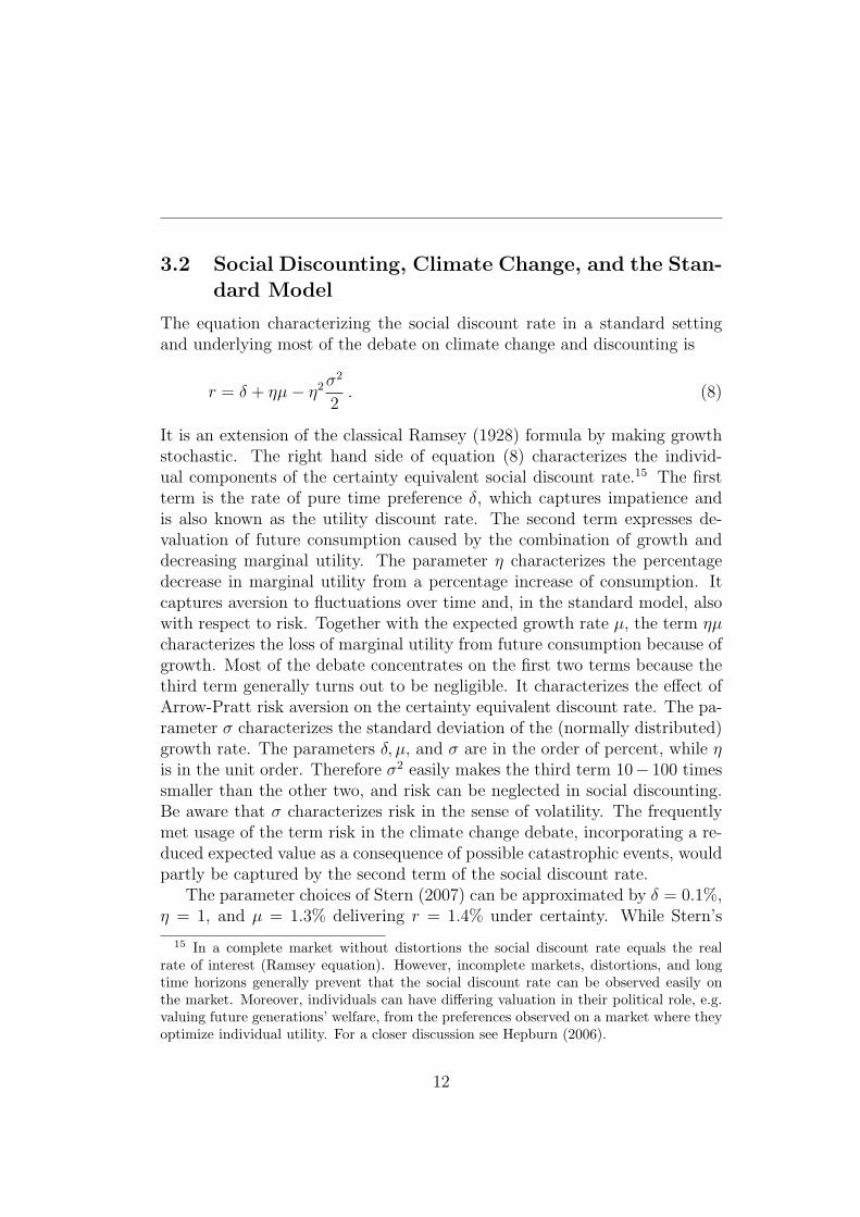
and discussed extensively in the recent debate, among others, by Nordhaus(2007), Weitzman (2007b) and Weitzman (2007a), and Dasgupta (2008b).A different adjustment stems from limited substitutability between goodsunder unbalanced growth as it can prevail for produced versus environmen-tal goods (Guesnerie 2004, Hoel & Sterner 2007, Traeger 2007d, Sterner &Persson 2008). After a brief introduction into the debate, this section dis-cusses the contribution of intertemporal risk aversion and ambiguous uncer-tainty to the social discount rate, two factors neglected in the current debate.

3.1 Setting

For the following analysis of social discount rates I assume isoelastic prefer-ences. The choice is based on three reasons. First, a constant intertemporalelasticity of substitution (CIES) in the standard model is a ubiquitous as-sumption in the social discounting debate. Second, isoelastic preferences incombination with normally distributed uncertainty make the model analyti-cally tractable. Third, for the case of intertemporal risk aversion, isoelasticityallows me to use estimates of intertemporal risk aversion based on the gen-eralized isoelastic model of Epstein & Zin (1989, 1991) and Weil (1990). Ianalyze a model with one aggregate commodity. Within a period utility fromcertain consumption is described by u(x) = xρ

ρwith ρ ≤ 1, ρ 6= 0. I am inter-

ested in the social discount rate for a stochastic growth scenario. Given somex1 the model assumes that the consumption growth rate g = ln x2

x1is normally

distributed with g ∼ N(µ, σ2). In section 3.3 the expected growth param-eter µ will be known, while in section 3.4 it will be probabilistic (Bayesianprior). The certainty equivalent consumption discount rate is defined asr = ln dx2

−dx1|U characterizing a marginal trade-off between the future (dx2)

and the present (dx1) that leaves overall welfare unchanged. The pure rateof time preference is δ = ln β. The consumption elasticity of marginal utilitybecomes η = 1 − ρ.

11

3.2 Social Discounting, Climate Change, and the Stan-

dard Model

The equation characterizing the social discount rate in a standard settingand underlying most of the debate on climate change and discounting is

r = δ + ηµ − η2σ2

2. (8)

It is an extension of the classical Ramsey (1928) formula by making growthstochastic. The right hand side of equation (8) characterizes the individ-ual components of the certainty equivalent social discount rate.15 The firstterm is the rate of pure time preference δ, which captures impatience andis also known as the utility discount rate. The second term expresses de-valuation of future consumption caused by the combination of growth anddecreasing marginal utility. The parameter η characterizes the percentagedecrease in marginal utility from a percentage increase of consumption. Itcaptures aversion to fluctuations over time and, in the standard model, alsowith respect to risk. Together with the expected growth rate µ, the term ηµ

characterizes the loss of marginal utility from future consumption because ofgrowth. Most of the debate concentrates on the first two terms because thethird term generally turns out to be negligible. It characterizes the effect ofArrow-Pratt risk aversion on the certainty equivalent discount rate. The pa-rameter σ characterizes the standard deviation of the (normally distributed)growth rate. The parameters δ, µ, and σ are in the order of percent, while η

is in the unit order. Therefore σ2 easily makes the third term 10− 100 timessmaller than the other two, and risk can be neglected in social discounting.Be aware that σ characterizes risk in the sense of volatility. The frequentlymet usage of the term risk in the climate change debate, incorporating a re-duced expected value as a consequence of possible catastrophic events, wouldpartly be captured by the second term of the social discount rate.

The parameter choices of Stern (2007) can be approximated by δ = 0.1%,η = 1, and µ = 1.3% delivering r = 1.4% under certainty. While Stern’s

15 In a complete market without distortions the social discount rate equals the realrate of interest (Ramsey equation). However, incomplete markets, distortions, and longtime horizons generally prevent that the social discount rate can be observed easily onthe market. Moreover, individuals can have differing valuation in their political role, e.g.valuing future generations’ welfare, from the preferences observed on a market where theyoptimize individual utility. For a closer discussion see Hepburn (2006).

12

team clearly argues for a normative dimension of these choices, the major-ity of integrated assessment modelers refuses such a standpoint.16 For thissecond group, Nordhaus, creator of the widespread open source integratedassessment model DICE is somewhat representative, adhering to a strictlypositive perspective. His parameter choices in the recent version of DICE-2007 (Nordhaus 2008) are δ = 1.5%, η = 2, and µ = 2%17 delivering r = 5.5%(again under certainty). Introducing uncertainty with a standard deviationof σ = 2% to the model would result in an adjustment of the risk free rateby 0.02% in the case of Stern and 0.08% in the case of Nordhaus, both neg-ligible. A standard deviation of σ = 2% is used by Weitzman (2009) toapproximate the volatility of economic growth without climate change andpossible catastrophic risks. The next section continues the discussion of theeffect of uncertainty in the face of climate change. I close with a recent illus-tration by Nordhaus (2007) on the importance of the social discount rate inclimate change evaluation. The author runs the DICE-2007 with both, theStern (2007) (r = 1.4%) parameterization of the social discount rate and hisown (r = 5.5%). These different parameterizations cause a difference in theoptimal reduction rate of emissions in the period 2010 − 2019 of 53% versus14% and a difference in the optimal carbon tax of 360$ versus 35$ per tonC.

3.3 The Social Discount Rate under Intertemporal Risk

Aversion

This section complements the recent debate on the social discount rate inthe face of climate change by incorporating the concept of intertemporal riskaversion. To match the generalized isoelastic model by Epstein & Zin (1989,1990) and Weil (1990) I pick intertemporal risk aversion of the isoelastic form

f(z) = (ρz)αρ

which returns a constant coefficient of relative Arrow Pratt risk aversion ofRRA = 1 − α that can be read off from the relation uvNM = f ◦ u(x) = xα.

16Moreover, Dasgupta (2008a) points out that, from a normative perspective, an egal-itarian choice of δ = 0.1% should as well call for a higher propensity of intergenerationalconsumption smoothing η > 1.

17The growth rate is endogenous in the DICE model and has been reconstructed fromNordhaus (2007, 694).

13

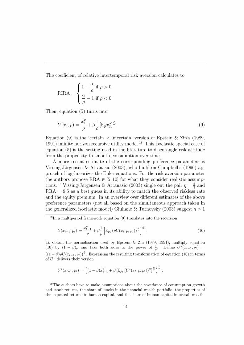
The coefficient of relative intertemporal risk aversion calculates to

RIRA =

1 −α

ρif ρ > 0

α

ρ− 1 if ρ < 0

Then, equation (5) turns into

U(x1, p) =x

ρ1

ρ+ β

1

ρ[Epx

α2 ]

ρα . (9)

Equation (9) is the ‘certain × uncertain’ version of Epstein & Zin’s (1989,1991) infinite horizon recursive utility model.18 This isoelastic special case ofequation (5) is the setting used in the literature to disentangle risk attitudefrom the propensity to smooth consumption over time.

A more recent estimate of the corresponding preference parameters isVissing-Jørgensen & Attanasio (2003), who build on Campbell’s (1996) ap-proach of log-linearizes the Euler equations. For the risk aversion parameterthe authors propose RRA ∈ [5, 10] for what they consider realistic assump-tions.19 Vissing-Jørgensen & Attanasio (2003) single out the pair η = 2

3and

RRA = 9.5 as a best guess in its ability to match the observed riskless rateand the equity premium. In an overview over different estimates of the abovepreference parameters (not all based on the simultaneous approach taken inthe generalized isoelastic model) Giuliano & Turnovsky (2003) suggest η > 1

18In a multiperiod framework equation (9) translates into the recursion

U(xt−1, pt) =xρ

t−1

ρ+ β

1

ρ

[

Ept(ρU(xt, pt+1))

αρ

]

ρ

α

, (10)

To obtain the normalization used by Epstein & Zin (1989, 1991), multiply equation(10) by (1 − β)ρ and take both sides to the power of 1

ρ. Define U∗(xt−1, pt) =

((1 − β)ρU(xt−1, pt))1

ρ . Expressing the resulting transformation of equation (10) in termsof U∗ delivers their version

U∗(xt−1, pt) =(

(1 − β)xρ

t−1 + β [Ept(U∗(xt, pt+1))

α]

ρ

α

)1

ρ

.

19The authors have to make assumptions about the covariance of consumption growthand stock returns, the share of stocks in the financial wealth portfolio, the properties ofthe expected returns to human capital, and the share of human capital in overall wealth.

14

and RRA > 2. All of these papers reject the standard model with its un-derlying assumption that α = ρ ⇔ RRA = η.20 The precise estimation ofthese preference characteristics stays a challenge for econometric analysis,and might also have to be extended beyond the isoelastic special case. Forthe present discussion I will use Vissing-Jørgensen & Attanasio’s (2003) bestguess of η = 2

3and RRA = 9.5. It implies a coefficient of relative intertem-

poral risk aversion RIRA = 26.5 (and furthermore η2 = 49

and |1 − η2| = 59).

Subsequently, I will employ two exemplary parameter sets based on Giuliano& Turnovsky’s (2003) survey for a ‘sensitivity check’.

Proposition 2: The certainty equivalent social discount rate in the isoelas-tic setting with intertemporal risk aversion is

r = δ + ηµ − η2σ2

2− RIRA

∣

∣1 − η2∣

∣

σ2

2. (11)

For a decision maker with positive intertemporal risk aversion RIRA > 0the value of the random future income stream is reduced. In consequence,an intertemporal risk averse decision maker is willing to invest into certainprojects with a relatively lower productivity than a decision maker who baseshis decision on the standard model.

Now the parameter η only reflects aversion to intertemporal fluctuations.Therefore the term η2 σ2

2should be interpreted as the cost of expected fluctu-

ations triggered by the aversion to non-smooth intertemporal consumptionpaths. I will still refer to the expression as ‘the standard risk term’, as itis the only expression capturing risk in an analysis based on the standardmodel (where η carries a double role). For my parametric best guess based onVissing-Jørgensen & Attanasio (2003), the importance of the intertemporalrisk aversion term in the social discount rate with respect to the standardrisk term is represented by the ratio

RIRA |1 − η2| σ2

2

η2 σ2

2

≈ 33 .

20The only empirical analysis of the generalizes isoelastic model I am aware of notrejecting the intertemporally additive expected utility special case is Normandin & St-Amour (1998).

15

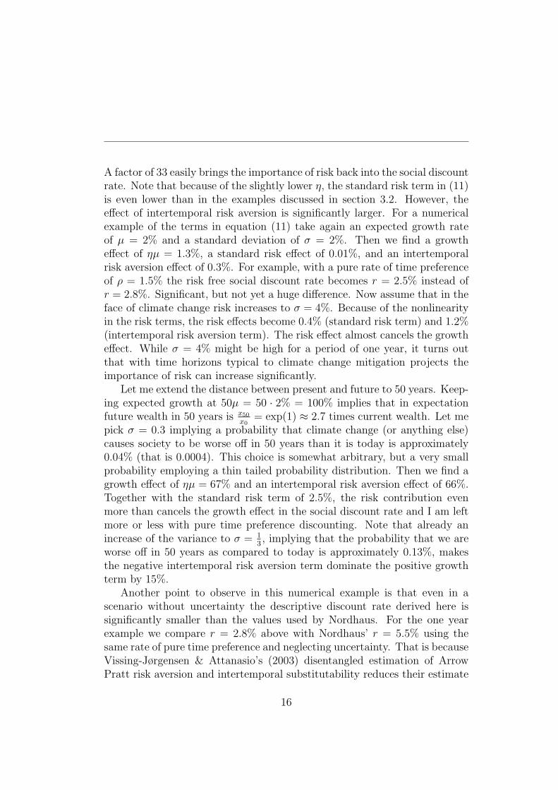
A factor of 33 easily brings the importance of risk back into the social discountrate. Note that because of the slightly lower η, the standard risk term in (11)is even lower than in the examples discussed in section 3.2. However, theeffect of intertemporal risk aversion is significantly larger. For a numericalexample of the terms in equation (11) take again an expected growth rateof µ = 2% and a standard deviation of σ = 2%. Then we find a growtheffect of ηµ = 1.3%, a standard risk effect of 0.01%, and an intertemporalrisk aversion effect of 0.3%. For example, with a pure rate of time preferenceof ρ = 1.5% the risk free social discount rate becomes r = 2.5% instead ofr = 2.8%. Significant, but not yet a huge difference. Now assume that in theface of climate change risk increases to σ = 4%. Because of the nonlinearityin the risk terms, the risk effects become 0.4% (standard risk term) and 1.2%(intertemporal risk aversion term). The risk effect almost cancels the growtheffect. While σ = 4% might be high for a period of one year, it turns outthat with time horizons typical to climate change mitigation projects theimportance of risk can increase significantly.

Let me extend the distance between present and future to 50 years. Keep-ing expected growth at 50µ = 50 · 2% = 100% implies that in expectationfuture wealth in 50 years is x50

x0= exp(1) ≈ 2.7 times current wealth. Let me

pick σ = 0.3 implying a probability that climate change (or anything else)causes society to be worse off in 50 years than it is today is approximately0.04% (that is 0.0004). This choice is somewhat arbitrary, but a very smallprobability employing a thin tailed probability distribution. Then we find agrowth effect of ηµ = 67% and an intertemporal risk aversion effect of 66%.Together with the standard risk term of 2.5%, the risk contribution evenmore than cancels the growth effect in the social discount rate and I am leftmore or less with pure time preference discounting. Note that already anincrease of the variance to σ = 1

3, implying that the probability that we are

worse off in 50 years as compared to today is approximately 0.13%, makesthe negative intertemporal risk aversion term dominate the positive growthterm by 15%.

Another point to observe in this numerical example is that even in ascenario without uncertainty the descriptive discount rate derived here issignificantly smaller than the values used by Nordhaus. For the one yearexample we compare r = 2.8% above with Nordhaus’ r = 5.5% using thesame rate of pure time preference and neglecting uncertainty. That is becauseVissing-Jørgensen & Attanasio’s (2003) disentangled estimation of ArrowPratt risk aversion and intertemporal substitutability reduces their estimate

16

of η and, thus, the growth effect. In an entangled approach to estimatingobserved preferences part of what is risk aversion RRA is falsely attributed tothe aversion to intertemporal fluctuations η overestimating the growth effectand the social discount rate.

While Vissing-Jørgensen & Attanasio’s (2003) estimate corresponds tothe case where η < 1, a literature survey by Giuliano & Turnovsky (2003) pro-poses η > 1 along with values RRA > 2. Building on Giuliano & Turnovsky(2003) let me exchange Vissing-Jørgensen & Attanasio’s (2003) value of η = 2

3

by Nordhaus’s (2008) value of η = 2. Keeping RRA = 9.5, which lies clearlyin the range suggested by Giuliano & Turnovsky (2003), reduces the coeffi-cient of relative intertemporal risk aversion to RIRA = 7.5. In the one yearscenario with µ = σ = 2% the growth effect grows back to Nordhaus’ 4%and standard and intertemporal risk aversion cut it back by .5%. Increasingthe variance to σ = 4% increases the negative risk effect to 2.1%, roughlyhalf of the growth effect. The same is true in the 50 year scenario withσ = .3 where the growth effect becomes 2 in the social discount rate andstandard risk aversion respectively intertemporal risk aversion cut it back by.18 respectively 1.

Stacking the deck further against the effects of intertemporal risk aversionlet me reduce the Arrow Pratt coefficient to RRA = 5, implying a furtherreduction of intertemporal risk aversion to RIRA = 3. In the one yearscenario with µ = σ = 2% the risk terms cut back less than .3% of the 4%growth term. With the one year σ = 4% scenario as well as in the 50 yearscenario the risk terms cut back on the social discount rate by a little morethan a quarter of the growth effect (1% and .59 respectively). Note thathere the standard risk effect with .18 is of similar order as the intertemporalrisk aversion effect with .41, a consequence of the relatively high aversionto intertemporal substitution and the low coefficient of intertemporal riskaversion.

The precise estimation of the parameters η and RRA, respectively RIRA,remains a challenge and the values calculated here are to be taken only as anindicator that we are likely to miss an important contribution to the socialdiscount rate by neglecting intertemporal risk aversion in the intertemporallyadditive standard model.

17

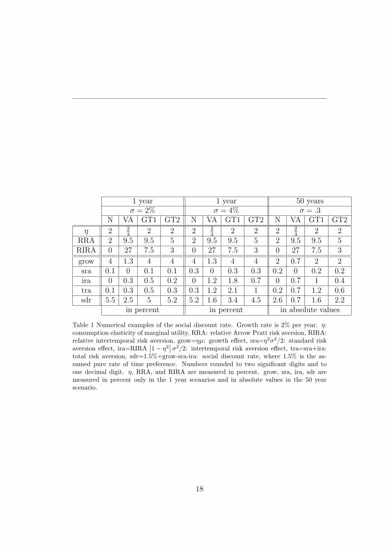
1 year 1 year 50 yearsσ = 2% σ = 4% σ = .3

N VA GT1 GT2 N VA GT1 GT2 N VA GT1 GT2

η 2 23

2 2 2 23

2 2 2 23

2 2RRA 2 9.5 9.5 5 2 9.5 9.5 5 2 9.5 9.5 5RIRA 0 27 7.5 3 0 27 7.5 3 0 27 7.5 3

grow 4 1.3 4 4 4 1.3 4 4 2 0.7 2 2sra 0.1 0 0.1 0.1 0.3 0 0.3 0.3 0.2 0 0.2 0.2ira 0 0.3 0.5 0.2 0 1.2 1.8 0.7 0 0.7 1 0.4tra 0.1 0.3 0.5 0.3 0.3 1.2 2.1 1 0.2 0.7 1.2 0.6sdr 5.5 2.5 5 5.2 5.2 1.6 3.4 4.5 2.6 0.7 1.6 2.2

in percent in percent in absolute values

Table 1 Numerical examples of the social discount rate. Growth rate is 2% per year. η:consumption elasticity of marginal utility, RRA: relative Arrow Pratt risk aversion, RIRA:relative intertemporal risk aversion, grow=ηµ: growth effect, sra=η2σ2/2: standard riskaversion effect, ira=RIRA

∣

∣1 − η2∣

∣ σ2/2: intertemporal risk aversion effect, tra=sra+ira:total risk aversion, sdr=1.5%+grow-sra-ira: social discount rate, where 1.5% is the as-sumed pure rate of time preference. Numbers rounded to two significant digits and toone decimal digit. η, RRA, and RIRA are measured in percent. grow, sra, ira, sdr aremeasured in percent only in the 1 year scenarios and in absolute values in the 50 yearscenario.

18

3.4 The Social Discount Rate under Ambiguity Aver-

sion

This section derives the effects of ambiguity aversion on social discounting.Weitzman (2009) recently argued that in the context of climate change theparameters of the distribution governing the growth process might not beknown. Like Weitzman, I adopt a Bayesian setting to capture such a formof second order uncertainty. While Weitzman sticks with the standard riskevaluation model underlying (8), in contrast, I adopt the ambiguity model byKlibanoff et al. (2005,2009) summarized in equation (7). Taking the simplestexample of Bayesian second order uncertainty, I assume that expected growthis itself a normally distributed parameter θ with expectation µ and varianceτ 2. Formally that is E(g|θ) ∼ N(θ, σ2) and θ ∼ N(µ, τ 2), preserving theinterpretation of µ as characterizing the overall expectation of the growthtrend. For a given realization of θ the standard deviation of the growthprocess stays a known parameter θ as in the previous model. Moreover, Iassume isoelasticity of ambiguity aversion Φ(z) = (ρz)ϕ yielding a constantcoefficient of relative ambiguity aversion

RAA =

{

1 − ϕ if ρ > 0

ϕ − 1 if ρ < 0

Under the assumptions summarized in section 3.1 the appendix derives thecorresponding social discount rate.

Proposition 3: The certainty equivalent social discount rate in the above 2period setting with constant relative ambiguity aversion and isoelasticutility is

r = δ + ηµ − η2σ2 + τ 2

2− RAA

∣

∣1 − η2∣

∣

τ 2

2. (12)

The first two terms reflect once more the discount rate as in the standardRamsey equation under certainty, the third term −η2 σ2+τ2

2reflects the well

known extension for risk, and the third term replaces the intertemporal riskaversion term and, here, is caused by ambiguity aversion. This new termreduces the certainty equivalent consumption discount rate and is propor-tional to relative ambiguity aversion and to second order variance τ 2. Under

19

ambiguity, the decision maker is willing to invest into certain projects withrelatively lower productivity than is a decision maker who is ambiguity neu-tral or just faces (first order) risk. In contrast to the model of intertemporalrisk aversion, the consumption discount rate is only reduced for second orderuncertainty (τ 2), not for objective first order risk (σ2).

Relating my results to Weitzman (2009) let me ignore ambiguity aversionand the term containing RAA. The only difference between the remainingpart of equation (12) and the standard equation (8) is the additional vari-ance τ in the third term on the right hand side (standard risk term). It is astraight forward consequence of making the growth process more uncertainby introducing a prior (second order uncertainty) over some parameter ofthe growth process. In the case of the normal distributions adopted here,the variance simply adds up. From the given example, it is hard to see howadding a Bayesian prior would bring the standard risk term back into theorder of magnitude needed to compare to the other characterizing terms ofthe social discount rate. Instead of a doubling, a factor of 10−100 is needed.The only way to reach this result is by sufficiently increasing the variance ofthe prior. Effectively, this is what Weitzman (2009) does in deriving whathe calls a dismal theorem. He introduces a fat tailed ignorant prior whosehigher moments do not exist. In consequence, the risk free social discountrate in equation (12) goes to minus infinity implying an infinite willingnessto transfer (certain) consumption into the future. Weitzman limits this will-ingness by the value of a (or society’s) statistical life.21 Instead of messingwith infinity, the above proposition follows the more humble approach ofintroducing ambiguity aversion, i.e. the term RAA |1 − η2| τ2

2, into social dis-

counting, reflecting experimental evidence that economic agents tend to bemore afraid of unknown probabilities than they are of known probabilities(most famously Ellsberg 1961). Unfortunately, I am not yet aware of es-timates for the parameter RAA in the Klibanoff et al. model. It will beinteresting whether ambiguity aversion can bring uncertainty back into thesocial discounting debate as well.

21 Note that Weitzman (2009) puts the prior on the variance σ rather than on theexpected value of growth. He loosely relates the uncertainty to climate sensitivity. Ofcourse, the above is a simplified perspective on Weitzman’s sophisticated approach.

20

4 Conclusions

Environmental and resource economics is largely an economics of long timehorizons and uncertainty. This fact is crucial to almost any aspect of theclimate change problem and just as important in more traditional problemslike the cost benefit analysis of biodiversity conservation. The recent discus-sion of the Stern review on climate policy has put a spotlight on a particu-larly important aspect of intertemporal evaluation: the social discount rate.Thereby, most of the discussion is framed in a standard discounted expectedutility setting. I have pointed out limitations of the standard model andcomplemented the discussion by deriving two new contributions to the socialdiscount rate that had been overlooked in the debate. One such contributionstems from the fact that the intertemporally additive expected utility modelcontains an implicit assumption of risk neutrality and the other contributionstems from additional aversion against ambiguous uncertainty.

In ‘certain×uncertain’ setting I develop a simplified characterization ofintertemporal risk aversion, characterizing the type of risk aversion that ismissing in the standard model. I show analytically how in a comprehensiveframework the social discount rate is reduced by a term proportional tointertemporal risk aversion. In a second extension of the standard modelI account for aversion to ambiguity, or aversion to ‘uncertainty about thecorrect probabilities’. Again, I analytically derive a term that reduces thesocial discount rate in the more comprehensive model. I find that the term isproportional to relative ambiguity aversion and identical in structure to theterm translating intertemporal risk aversion into the social discount rate.

I use estimates of Epstein & Zin’s (1989) and Weil’s (1990) generalizedisoelastic model to analyze the quantitative importance of intertemporal riskaversion in the social discount rate. I find that under intertemporal riskaversion the influence of risk (volatility), which is negligible in the standardmodel, comes back into the same order of magnitude as the much discussedvalues for growth discounting and pure time preference. Based on a bestguess by Vissing-Jørgensen & Attanasio (2003) I show that, under moderateassumptions about climate risk, the risk contribution to social discountingcan quantitatively cancel the growth contribution. Then, the social discountrate coincides with pure time preference. Analyzing the contribution of twoother guesstimates yielding lower coefficients of intertemporal risk aversion,I still find that the contribution to the social discount rate is significantand should not be neglected. A different insight is that the ability of the

21

model to disentangle attitude with respect to time and with respect to risktends to lower the growth contribution to social discounting. The reason isthat in the standard model willingness to smooth consumption over time isoverestimated as it is described by the same coefficient that has to capture(the generally higher) Arrow Pratt risk aversion. Both effects reduce thecertainty equivalent discount rate. In consequence, projects should be carriedout that in a cost benefit analysis based on the standard model would bediscounted into inefficiency.

While a reliable quantification of the contributions derived in this pa-per is yet to be obtained, the theoretical insights should be kept in mindwhen formulating long-term policies, in particular, if they involve a tradeof between long-run, high uncertainty scenarios versus scenarios promisinga more stable development, e.g. of our current climate. A crucial aspectof the climate change problem is that we are learning at a fast speed overthe consequences, the technical mitigation possibilities, and at least some ofthe economic uncertainties involved in climate change. Thus, an importantextension of the model will be the incorporation of an arbitrary time horizonin combination with the anticipation of learning.

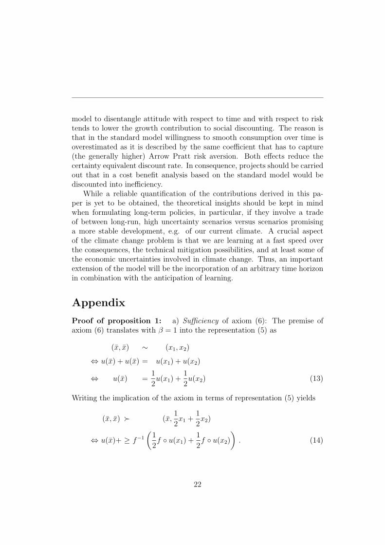
Appendix

Proof of proposition 1: a) Sufficiency of axiom (6): The premise ofaxiom (6) translates with β = 1 into the representation (5) as

(x, x) ∼ (x1, x2)

⇔ u(x) + u(x) = u(x1) + u(x2)

⇔ u(x) =1

2u(x1) +

1

2u(x2) (13)

Writing the implication of the axiom in terms of representation (5) yields

(x, x) ≻ (x,1

2x1 +

1

2x2)

⇔ u(x)+ ≥ f−1

(

1

2f ◦ u(x1) +

1

2f ◦ u(x2)

)

. (14)

22

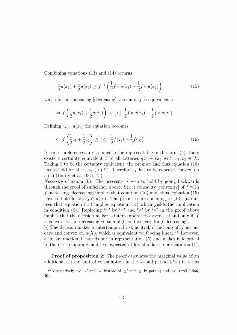
Combining equations (13) and (14) returns

1

2u(x1) +

1

2u(x2) ≥ f−1

(

1

2f ◦ u(x1) +

1

2f ◦ u(x2)

)

(15)

which for an increasing [decreasing] version of f is equivalent to

⇔ f

(

1

2u(x1) +

1

2u(x2)

)

> [<]1

2f ◦ u(x1) +

1

2f ◦ u(x2) .

Defining zi = u(xi) the equation becomes

⇔ f

(

1

2z1 +

1

2z2

)

≥ [≤]1

2f(z1) +

1

2f(z2) . (16)

Because preferences are assumed to be representable in the form (5), thereexists a certainty equivalent x to all lotteries 1

2x1 + 1

2x2 with x1, x2 ∈ X.

Taking x to be the certainty equivalent, the premise and thus equation (16)has to hold for all z1, z2 ∈ u(X). Therefore, f has to be concave [convex] onU(x) (Hardy et al. 1964, 75).Necessity of axiom (6): The necessity is seen to hold by going backwardsthrough the proof of sufficiency above. Strict concavity [convexity] of f withf increasing [decreasing] implies that equation (16) and, thus, equation (15)have to hold for z1, z2 ∈ u(X). The premise corresponding to (13) guaran-tees that equation (15) implies equation (14) which yields the implicationin condition (6). Replacing ‘�’ by ‘�’ and ‘≥’ by ‘≤’ in the proof aboveimplies that the decision maker is intertemporal risk averse, if and only if, f

is convex [for an increasing version of f , and concave for f decreasing].b) The decision maker is intertemporal risk neutral, if and only if, f is con-cave and convex on u(X), which is equivalent to f being linear.22 However,a linear function f cancels out in representation (5) and makes it identicalto the intertemporally additive expected utility standard representation (1).

Proof of proposition 2: The proof calculates the marginal value of anadditional certain unit of consumption in the second period (dx2) in terms

22Alternatively use ‘∼’ and ‘=’ instead of ‘�’ and ‘≥’ in part a) and use Aczel (1966,46).

23

of first period consumption (dx1)

V (x1, I1) =x

ρ1

ρ+ β

1

ρ

[

EP (x2|x1,I1)xα2

]ρα

⇒ dV (x1, I1) = xρ−11 dx1 + β

1

α

[

EP (x2|x1,I1)xα2

]ρα−1

EP (x2|x1,I1)αxα−12 dx2

!= 0

⇒ xρ−11 dx1 = −β

[

EP (x2|x1,I1)xα2

]ρα−1

EP (x2|x1,I1)xα−12 dx2

⇒dx1

dx2

= −β

[

EP (x2|x1,I1)

(

x2

x1

)α ]

ρα−1

EP (x2|x1,I1)

(

x2

x1

)α−1

⇒dx1

dx2

= −β[

EP (x2|x1,I1)eα ln

x2x1

]ρα−1

EP (x2|x1,I1)e(α−1) ln

x2x1

⇒dx1

dx2

= −β[

eαµ+α2 σ2

2

]

ρα−1

e(α−1)µ+(1−α)2 σ2

2

⇒dx1

dx2

= −βeρµ+αρ σ2

2−αµ−α2 σ2

2 e(α−1)µ+(1−α)2 σ2

2

⇒dx1

dx2

= −βe(ρ−1)µ+(αρ+1−2α)σ2

2

⇒dx1

dx2

= −βe(ρ−1)µ+(αρ+1−2α)σ2

2 .

With the definitions r = − ln dx1

−dx2

(

= ln dx2

−dx1|V

)

, δ = ln β, η = 1− ρ(

= 1σ

)

,

24

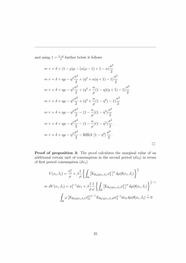
and using 1 = 1−η

ρfurther below it follows

⇒ r = δ + (1 − ρ)µ − (α(ρ − 1) + 1 − α)σ2

2

⇒ r = δ + ηµ − η2σ2

2+ (η2 + α(η + 1) − 1)

σ2

2

⇒ r = δ + ηµ − η2σ2

2+ (η2 +

α

ρ(1 − η)(η + 1) − 1)

σ2

2

⇒ r = δ + ηµ − η2σ2

2+ (η2 +

α

ρ(1 − η2) − 1)

σ2

2

⇒ r = δ + ηµ − η2σ2

2− (1 −

α

ρ)(1 − η2)

σ2

2

⇒ r = δ + ηµ − η2σ2

2− (1 −

α

ρ)(1 − η2)

σ2

2.

⇒ r = δ + ηµ − η2σ2

2− RIRA

∣

∣1 − η2∣

∣

σ2

2.

�

Proof of proposition 3: The proof calculates the marginal value of anadditional certain unit of consumption in the second period (dx2) in termsof first period consumption (dx1)

V (x1, I1) =x

ρ1

ρ+ β

1

ρ

{∫

Θ

[

EΠθ(y|x1,I1)xρ2

]ϕdµ(θ|x1, I1)

}1

ϕ

⇒ dV (x1, I1) = xρ−11 dx1 + β

1

ρ

1

ϕ

{∫

Θ

[

EΠθ(y|x1,I1)xρ2

]ϕdµ(θ|x1, I1)

}1

ϕ−1

∫

Θ

ϕ[

EΠθ(y|x1,I1)xρ2

]ϕ−1EΠθ(y|x1,I1)ρx

ρ−12 dx2 dµ(θ|x1, I1)

!= 0

25

⇒ xρ−11 dx1 = −β

{∫

Θ

[

EΠθ(y|x1,I1)xρ2dx2

]ϕdµ(θ|x1, I1)

}1

ϕ−1

∫

Θ

[

EΠθ(y|x1,I1)xρ2

]ϕ−1EΠθ(y|x1,I1)x

ρ−12 dx2 dµ(θ|x1, I1)

⇒dx1

dx2

= −β

{∫

Θ

[

EΠθ(y|x1,I1)

(

x2

x1

)ρ ]ϕ

dµ(θ|x1, I1)

}1

ϕ−1

∫

Θ

[

EΠθ(y|x1,I1)

(

x2

x1

)ρ ]ϕ−1

EΠθ(y|x1,I1)

(

x2

x1

)ρ−1

dµ(θ|x1, I1)

⇒dx1

dx2

= −β

{∫

Θ

[

EΠθ(y|x1,I1)eρ ln

x2x1

]ϕ

dµ(θ|x1, I1)

}1

ϕ−1

∫

Θ

[

EΠθ(y|x1,I1)eρ ln

x2x1

]ϕ−1

EΠθ(y|x1,I1)e(ρ−1) ln

x2x1 dµ(θ|x1, I1)

⇒dx1

dx2

= −β

{∫

Θ

[

eρθ+ρ2 σ2

2

]ϕ

dµ(θ|x1, I1)

}1

ϕ−1

∫

Θ

[

eρθ+ρ2 σ2

2

]ϕ−1

e(ρ−1)θ+(ρ−1)2 σ2

2 dµ(θ|x1, I1)

⇒dx1

dx2

= −βe[(1−ϕ)ρ2+(ϕ−1)ρ2+(ρ−1)2]σ2

2

{∫

Θ

[

eρθϕ]

dµ(θ|x1, I1)

}1

ϕ−1

∫

Θ

[

eρθ(ϕ−1)]

e(ρ−1)θdµ(θ|x1, I1)

⇒dx1

dx2

= −βe(ρ−1)2 σ2

2

{∫

Θ

[

eρθϕ]

dµ(θ|x1, I1)

}1

ϕ−1

∫

Θ

eθ[ρϕ−ρ+ρ−1]dµ(θ|x1, I1)

26

⇒dx1

dx2

= −βe(ρ−1)2 σ2

2

{

eρϕµ+ρ2ϕ2 τ2

2

}

1

ϕ−1

[

e(ρϕ−1)µ+(ρϕ−1)2 τ2

2

]

⇒dx1

dx2

= −βe(ρ−1)2 σ2

2 e[ρ(1−ϕ)+ρϕ−1]µ

e[ρ2ϕ(1−ϕ)+ρ2ϕ2−2ρϕ+1] τ2

2

⇒dx1

dx2

= −βe(ρ−1)2 σ2

2 e(ρ−1)µe[ρ2ϕ−2ρϕ+ϕ−ϕ+1] τ2

2

⇒dx1

dx2

= −βe(ρ−1)2 σ2

2 e(ρ−1)µe[ϕ(ρ−1)2+(1−ϕ)] τ2

2

⇒dx1

dx2

= −βe−(1−ρ)µe(1−ρ)2 σ2+τ2

2 e[−(1−ϕ)(1−ρ)2+(1−ϕ)] τ2

2

or with r = ln dx2

−dx1|V , δ = − ln β, and η = 1 − ρ

r = δ + ηµ − η2σ2 + τ 2

2− (1 − ϕ)(1 − η2)

τ 2

2

= δ + ηµ − η2σ2 + τ 2

2− RAA

∣

∣1 − η2∣

∣

τ 2

2.

�

References

Aczel, J. (1966), Lectures on Functional Equations and their Applications,Academic Press, New York.

Campbell, J. Y. (1996), ‘Understanding risk and return’, The Journal of

Political Economy 104(2), 298–345.

Dasgupta, P. (2008a), ‘Commentary: The stern review’s economics of climatechange’. National Institute Economic Review 2007; 199; 4.

Dasgupta, P. (2008b), ‘Discounting climate change’. Working Paper.

27

Ellsberg, D. (1961), ‘Risk, ambiguity and the savage axioms’, Quarterly Jour-

nal of Economics 75, 643–69.

Epstein, L. G. & Zin, S. E. (1989), ‘Substitution, risk aversion, and the tem-poral behavior of consumption and asset returns: A theoretical frame-work’, Econometrica 57(4), 937–69.

Fishburn, P. C. (1992), ‘A general axiomatization of additive measurementwith applications’, Naval Research Logistics 39(6), 741–755.

Ghirardato, P., Maccheroni, F. & Marinacci, M. (2004), ‘Differentiat-ing ambiguity and ambiguity attitude’, Journal of Economic Theory

118(2), 122–173.

Gilboa, I. & Schmeidler, D. (1989), ‘Maxmin expected utility with non-unique prior’, Journal of Mathematical Economics 18(2), 141–53.

Giuliano, P. & Turnovsky, S. J. (2003), ‘Intertemporal substitution, riskaversion, and economic performance in a stochastically growing openeconomy’, Journal of International Money and Finance 22(4), 529–556.

Guesnerie, R. (2004), ‘Calcul economique et developpement durable’, Revue

economique 55(3), 363–382.

Hansen, L. P. & Sargent, T. J. (2001), ‘Robust control and model uncer-tainty’, American Economic Review 91(2), 60–66.

Hardy, G., Littlewood, J. & Polya, G. (1964), Inequalities, 2 edn, CambridgeUniversity Press. first puplished 1934.

Hepburn, C. (2006), Discounting climate change damages: Working notesfor the Stern review, Working note.

Hoel, M. & Sterner, T. (2007), ‘Discounting and relative prices’, Climatic

Change 84, 265–280.

Jaffray, J.-Y. (1974a), Existence. Proprietes de Conrinuie, Additivite deFonctions d’Utilite sur un Espace Partiellement ou Totalement Ordonne,PhD thesis, Universite der Paris, VI.

Jaffray, J.-Y. (1974b), ‘On the existence of additive utilities on infinite sets’,Journal of Mathematical Psychology 11(4), 431–452.

28

Kihlstrom, R. E. & Mirman, L. J. (1974), ‘Risk aversion with many com-modities’, Journal of Economic Theory 8(3), 361–88.

Klibanoff, P., Marinacci, M. & Mukerji, S. (2005), ‘A smooth model of deci-sion making under ambiguity’, Econometrica 73(6), 1849–1892.

Klibanoff, P., Marinacci, M. & Mukerji, S. (2006), Recursive smooth ambi-guity preferences, Carlo Alberto Notebooks 17, Collegio Carlo Alberto.

Klibanoff, P., Marinacci, M. & Mukerji, S. (2009), ‘Recursive smooth ambi-guity preferences’, Journal of Economic Theory 144, 930–976.

Koopmans, T. C. (1960), ‘Stationary ordinal utility and impatience’, Econo-

metrica 28(2), 287–309.

Krantz, D., Luce, R., Suppes, P. & Tversky, A. (1971), Foundations of mea-

surement. Vol. I. Additive and polynomial representaiions, AcademicPress, New York.

Kreps, D. M. & Porteus, E. L. (1978), ‘Temporal resolution of uncertaintyand dynamic choice theory’, Econometrica 46(1), 185–200.

Maccheroni, F., Marinacci, M. & Rustichini, A. (2006a), ‘Ambiguity aversion,robustness, and the variational representation of preferences’, Econo-

metrica 74(6), 1447–1498.

Maccheroni, F., Marinacci, M. & Rustichini, A. (2006b), ‘Dynamic varia-tional preferences’, Journal of Economic Theory 128(1), 4–44.

Nordhaus, W. (2008), A Question of Balance: Economic Modeling of Global

Warming, Yale University Press, New Haven. Online preprint: A Ques-tion of Balance: Weighing the Options on Global Warming Policies.

Nordhaus, W. D. (2007), ‘A review of the Stern review on the economics ofclimate change’, Journal of Economic Literature 45(3), 686–702.

Normandin, M. & St-Amour, P. (1998), ‘Substitution, risk aversion, tasteshocks and equity premia’, Journal of Applied Econometrics 13(3), 265–281.

29

Plambeck, E. L., Hope, C. & Anderson, J. (1997), ‘The Page95 model: Inte-grating the science and economics of global warming’, Energy Economics

19, 77–101.

Radner, T. (1982), Microeconomic Theory, Acedemic Press, New York.

Ramsey, F. P. (1928), ‘A mathematical theory of saving’, The Economic

Journal 38(152), 543–559.

Savage, L. J. (1954), The foundations of statistics, Wiley, New York.

Selden, L. (1978), ‘A new representation of preferences over’cerain×uncertain’ consumption pairs: The ’ordinal certainty equiva-lent’ hypothesis’, Econometrica 46(5), 1045–1060.

Stern, N., ed. (2007), The Economics of Climate Change: The Stern Review,Cambridge University Press, Cambridge.

Sterner, T. & Persson, M. (2008), ‘An even sterner review: Introducing rela-tive prices into the discounting debate’, Review of Environmental Eco-

nomics and Policy 2(1), 61–76.

Traeger, C. (2007a), Disentangling risk aversion from intertemporal substi-tutability and the temporal resolution of uncertainty. Working Paper.

Traeger, C. (2007b), The generalized isoelastic model for many commodities.Working Paper.

Traeger, C. (2007c), Intertemporal risk aversion, stationarity and the rate ofdiscount. Working Paper.

Traeger, C. (2007d), ‘Sustainability, limited substitutability and non-constant social discount rates’. CUDARE Working Paper 1045.

Traeger, C. (2007e), ‘Wouldn’t it be nice to know whether Robinson is riskaverse?’. Working Paper.

Vissing-Jørgensen, A. & Attanasio, O. P. (2003), ‘Stock-market participation,intertemporal substitution, and risk-aversion’, The American Economic

Review 93(2), 383–391.

30

von Neumann, J. & Morgenstern, O. (1944), Theory of Games and Economic

Behaviour, Princeton University Press, Princeton.

Wakker, P. (1988), ‘The algebraic versus the topological approach to additiverepresentations’, Journal of Mathematical Psychology 32, 421–435.

Weil, P. (1990), ‘Nonexpected utility in macroeconomics’, The Quarterly

Journal of Economics 105(1), 29–42.

Weitzman, M. (2007a), ‘Structural uncertainty and the value of statisticallife in the economics of catastrophic climate change’, (13490).

Weitzman, M. L. (2007b), ‘A review of the Stern review on the economics ofclimate change’, Journal of Economic Literature 45(3), 703–724.

Weitzman, M. L. (2009), ‘On modeling and interpreting the economics ofcatastrophic climate change’, The Review of Economics and Statistics

91(1), 1–19. 06.

31