the solar atmosphere - university corporation for ... solar atmosphere ... momentum and energy...

The Solar Atmosphere(as seen from the)

Institute of Theoretical Astrophysics, University of Oslo

Viggo H. Hansteen

QuickTime™ and aPhoto - JPEG decompressor

are needed to see this picture.

Sun: July 29, 1998 with TRACE 171Å

Solar Atmospheric structure:Expected dynamics and energetics

• The photosphere

• braiding of the magnetic field; injection of Poynting flux

• injection of acoustic flux

• The chromosphere

• conduit of waves and other motions

• region where

• The Transition Region and Corona

• deposition of energy flux

• diagnostic signatures of waves and heating

The Photosphere



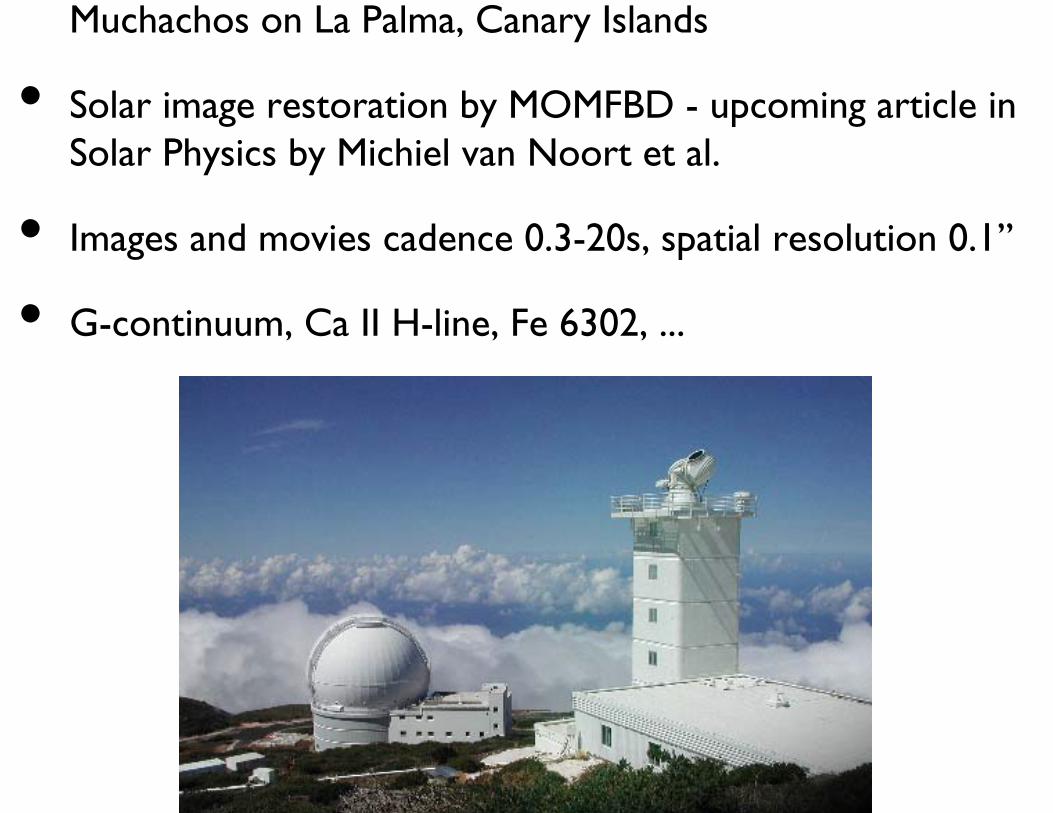
Muchachos on La Palma, Canary Islands

• Solar image restoration by MOMFBD - upcoming article in Solar Physics by Michiel van Noort et al.

• Images and movies cadence 0.3-20s, spatial resolution 0.1”

• G-continuum, Ca II H-line, Fe 6302, ...

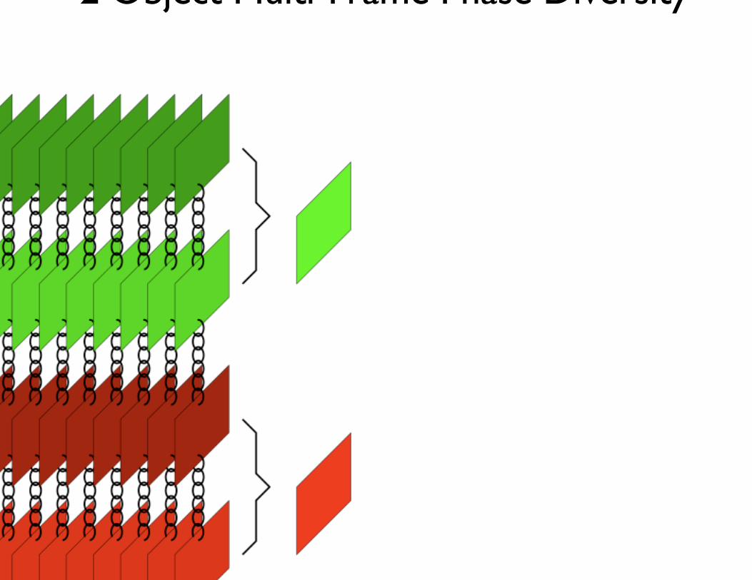
2 Object Multi Frame Phase Diversity

20 Aug 2004, G-band



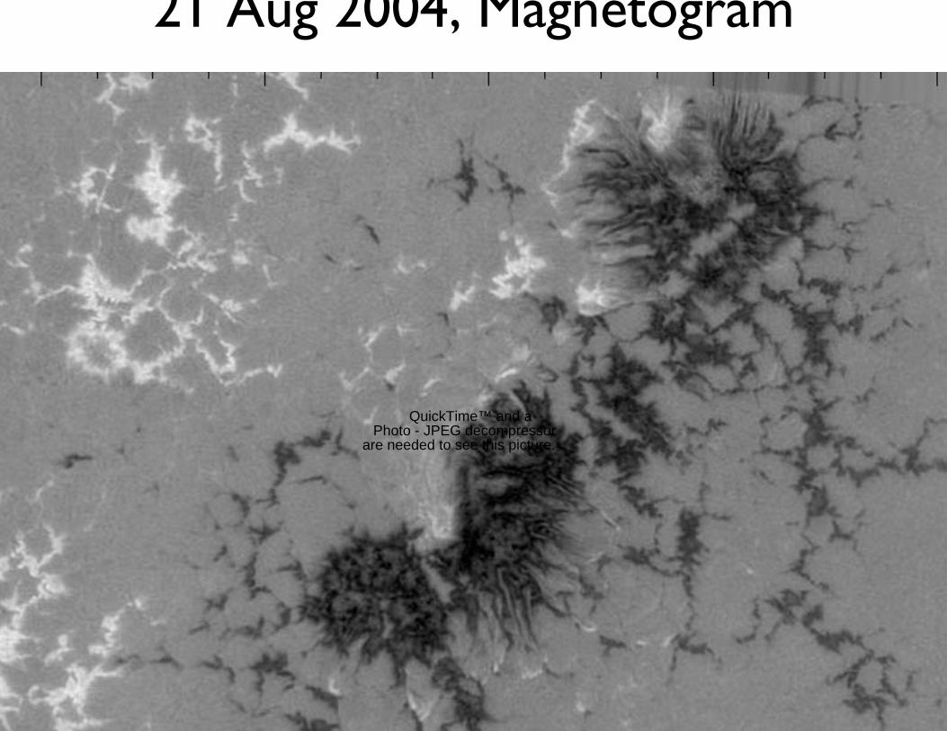
21 Aug 2004, Magnetogram



apan/US/UK mission (Norway, ESA)

Solar Optical Telescope

X-Ray Telescope

Extreme UV Imaging Spectrograph

��Hinode) Launch

eptember 23, 2006

Dec 13 2006, Hinode/SOT Flare

QuickTime™ and aSorenson Video 3 decompressorare needed to see this picture.

The MHD equations

some equation of state

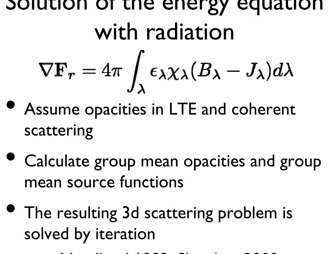
Solution of the energy equation with radiation

• Assume opacities in LTE and coherent scattering

• Calculate group mean opacities and group mean source functions

• The resulting 3d scattering problem is solved by iteration

N dl d 1982 Sk li 2000

g p

with etcthen

oup number defined by

• Nordlund/Stein code

• multi-group opacities, 4 bins

• Initial field 250G, vertical, single polarity

• 253x253x163 simulation

• RT each snapshot, 2728 frequency points

• Line blanketing: 845 lines

HD simulation of Solar magneto convecti

C l t l 2004 A J 610

imulation, mu=0.6 Observation, mu=0.6

Temperature structure

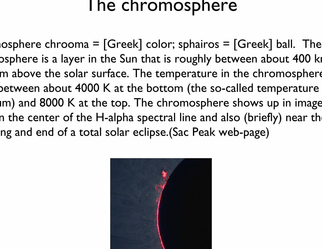
The chromosphere

mosphere chrooma = [Greek] color; sphairos = [Greek] ball. The osphere is a layer in the Sun that is roughly between about 400 kmm above the solar surface. The temperature in the chromospherebetween about 4000 K at the bottom (the so-called temperature um) and 8000 K at the top. The chromosphere shows up in imagen the center of the H-alpha spectral line and also (briefly) near theng and end of a total solar eclipse.(Sac Peak web-page)

QuickTime™ and aYUV420 codec decompressor


Ca II H as seen with Hinode

Chromospheric structure and oscillations

The internetwork chromosphere may perhaps be considered as a gravitationally stratified isothermal slab. In which case we may combine the linearized mass, momentum and energy equations.

QuickTime™ and aGIF decompressor


1D non-LTE simulation

Ca II H-line intensity

Semi-empirical equivalent

Wave energy flux as function of height



What have we learnt?

• Ca II grains explained by acoustic waves

• only way to get strong blue-red assymetry is through a strong velocity gradient

• 3 min waves present already in photosphere

• Non-magnetic chromosphere very dynamic. Theremay be no temperature rise.

• Slow rates important for hydrogen ionization and energy balance in chromosphere

• Acoustic waves not enough to explain mid-upper chromosphere in internetwork

d speed with periods of r 3 min/5 mHz

edicted by “Carlsson-Stein” type models ol. 397, no. 1, p. L59-L62)

d also observed at greater hts in the atmosphere... støl et al, 2000 (ApJ Volume 531, , pp. 1150-1160)

ever... the Sun has magnetic and more!!!

The chromospheric network

Network and inter-network

Magnetic flux tube

Radiative damping

Adiabatic, non-magnetic

Roberts, 1983, Solar Physics 87,77

y(McIntosh et al., 2001, ApJL 548, 237)

Weak field - vertical driving





Strong field - vertical driving

• Be aware of regions surrounding place where observations are obtained

• Observation made in high or low beta plasma?

• Closest approach of magnetic canopy

• Where magnetic field at measurement site connects to photosphere

• Location of wave source and dominant state of polarization

• Proximity may not be overriding factor...

• Understand that as many as three wave modes are moving information and energy

g

2D version



QuickTime™ and aH.264 decompressor


Diffraction limited (0 2”) Ha linecenter at 1 s cadence from 8:50 to 10:10 UT m=0 78 (S8 E37)

QuickTime™ and aCinepak decompressor


The life of a Dynamic Fibril

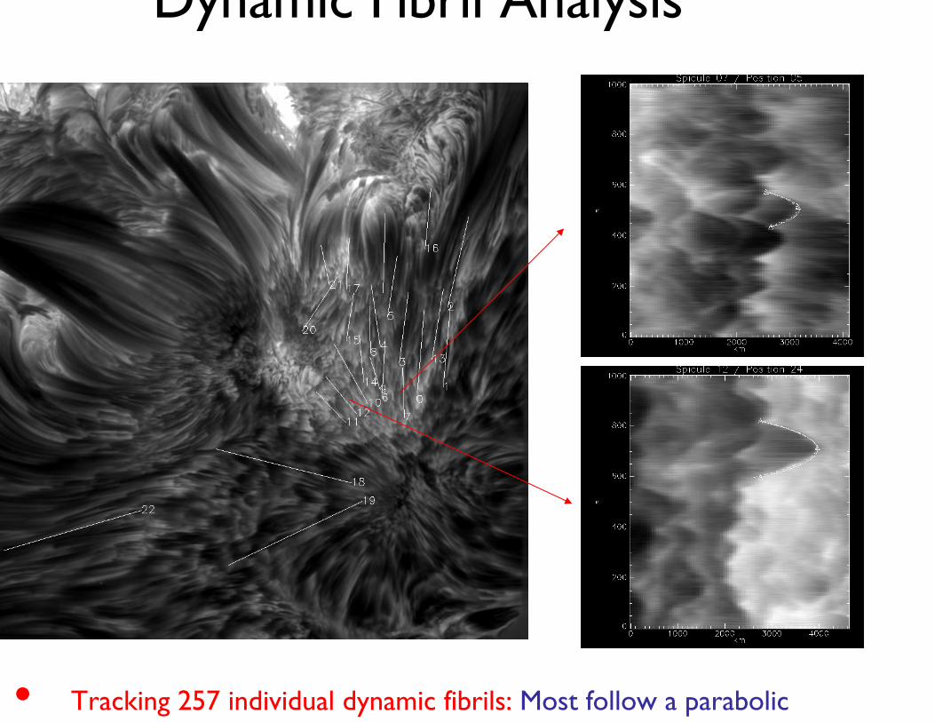
Dynamic Fibril Analysis

• Tracking 257 individual dynamic fibrils: Most follow a parabolic

• On average (but with large spread):

• Fast DFs are decelerated the most, and long DFs live the longest

Parabolas in Ca II H as observed with Hinode

QuickTime™ and aFoto - JPEG decompressor


Simulations: inclined field

Simulated log Tg and uz

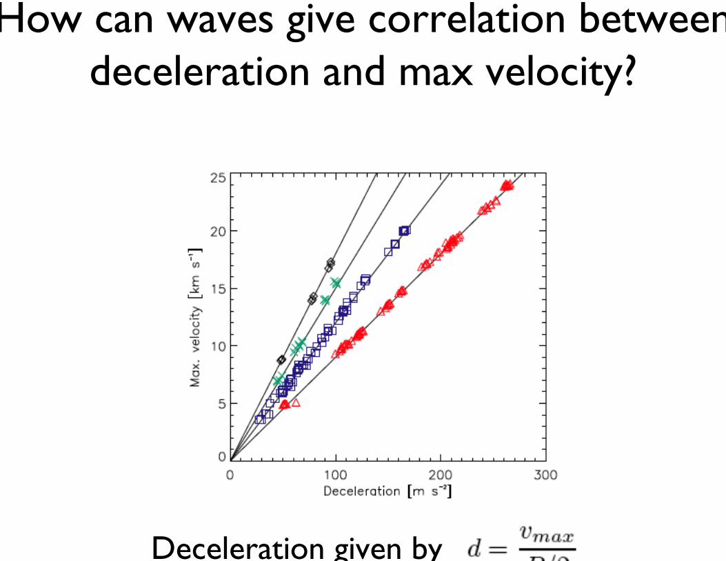
How can waves give correlation betweendeceleration and max velocity?

Deceleration given by

velocity/deceleration

Coronal Heating

Parker, E.N., 1991, Reviews in Modern Astronomy, p 1-17

Coronal heating questions

• AC or DC?

• Constant or episodic?

• How is energy flux thermalized?

• Need continual injection of new magnetic flux?

• Robust diagnostics that can separate various scenarios?

Nano , micro , and milliflares

Aschwanden et al., 2000, ApJ 535,

• Temperature set by balance of energy gains and losses

• Possible coronal energy losses are radiation, conduction, and solar wind acceleration

• Radiative losses given by

• Conduction given by

• Efficiency of conduction poor at low T, efficiency of radiation poor at low n

Why is the corona 1 MK?

Transition Region Structure

Line emission from the optically thin Transition Region

Warren, 2005, ApJSS 157, 147

The differential emission measure (DEM)

mperature gradient

oustic wave will partially oximately 50% of the wave y) reflect off the expected tion region temperature nt

tion will lead to phase shifts en line shifts and the line ities

show that...

the 5-10 mHz oscillations can be followed up into the (upper) tranregion

the oscillations are best seen in thshift, but are also present as variathe line intensity

Wikstøl et al, 2000 (ApJ Volume 531, Issue 2, pp. 1150-1160)

t, episodic events in the a should leave a trace in tion region emission

tion region jets, turbulent s and blinkers?

rhaps a “natural quence” of episodic g; gas is heated quickly

ools slowly as predicted by & Holzer 1982 and ps shown by Peter &

ksen 2005

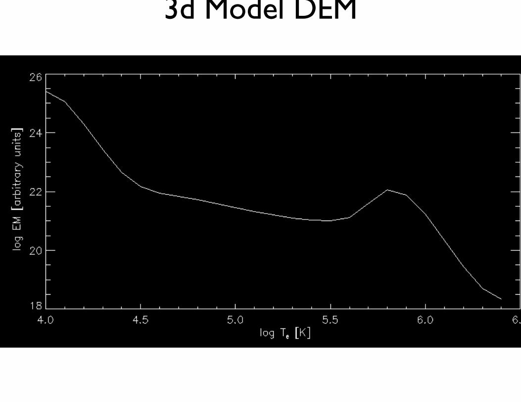
3d Model DEM

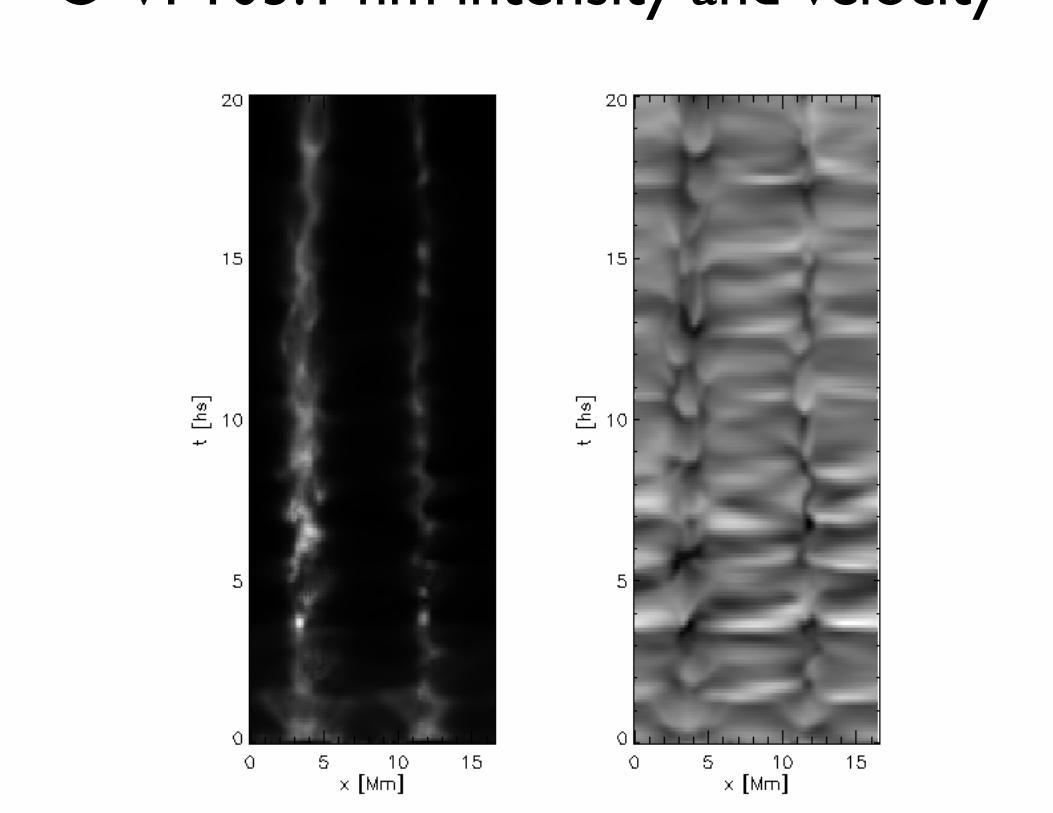
O VI 103.1 nm intensity and velocity

Average O VI 103.1 nm velocities

3d convection zone to coronal modeling

• Corona is high temperature and low beta

• thermal conduction dominates the energy equation

• heat flows along the field in low beta plasma

• Convection zone & photosphere is high beta

• Coronal dynamics and energetics are a result of forcing by the lower regions of the atmosphere

• Driving term in energy equation is radiation

• Chromosphere (and TR) are intermediate

The MHD equations

some equation of state

Solution of the energy equation with conduction

• Numerical analysis severely strained by Courant condition - which with conduction scales as the grid size squared

• An implicit operator to solve diffusive part of operator

• Proceed by operator splitting

• High order explicit method with Hyman time-stepping is used to solve MHD

• Multigrid method is used to solve diffusive operator

do it = 1, nstep

if (heatflux) call init_heat_flux

call mhd_timestep()

if (heatflux) call heat_flux_mg

...

Solution Strategy

a) Use Crank-Nicholson to discretize; compute explicit part of operatorb) Solve MHD part of operator by “usual” methodc) Update temperature by solving by multi-grid method

General considerations

which means solution converges by repeated averaging

Elliptic (and "elliptic like") operators can be solved by relaxation methods

e general idea is that Jacobi or Gauss - Seidel iteration is very gooremoving errors on the "small" scales and very bad at removing rors on "large" scales.

ultigrid methods work by converting large scales to small scales

g

• We use a V-cycle starting at original grid size h

• at this finest grid level the solution is smoothed using a few Gauss-Seidel relaxation to smooth the high frequency errors

• The residual errors are injected into a coarser grid

• This process of smoothing and injection continues down to a the coarsest grid

• The solution interpolated back up to the finest grid

• through a succession of intermediate smoothing and prolongation steps

• Injection and prolongation are obtained simply by bilinear interpolation.

Multigrid methods originally by Brandt 1977 (Mathematics of Computation, vol 31, pp 333-390)

Originally coded by A. Malagoli, A. Dubey, F. Cattaneo “A Portable and Efficient Parallel Code for Astrophysical Fluid Dynamics”

Models with photospheric driving

Gudiksen & Nordlund, 2002, ApJ 572, L113Gudiksen & Nordlund, 2005, ApJ 618, 1020

Driving via horizontal velocities

Driving based on observations & modeling at smallest scales



Trace 171Å emission

Gudiksen & Nordlund, 2002, ApJ 572, Gudiksen & Nordlund, 2005, ApJ 618, 1



Heating via magnetic dissipation

where the resistive part of the electric field is

where the diffusivities are given by



Ne VIII 77.4 nm



pt = 2000 s - 3600 s



O6O VI 103.1 nm

O VI 103.1 nm



realistic 3D simulations

Red field

Colorintempera

(red=chromoreen/blue=

Hansteen & C



• It seems we have a promising hypothesis...

• How do we test it?

• Peter Cargill’s cat can reproduce TRACE images...

• ...it would be interesting to investigate

• variations in the field strength

• variations in the initial field topology

• do we need to introduce new flux?

• is there any interaction between waves and dissipation?

• etc

( )

( )

• Our treatment of microscopic physics is wrong

• Does it matter? Galsgaard & Nordlund 1996 claim “No”

• Thermalization

• via particle acceleration (Turkmani et al.)

• via highly episodic scale phenomena (Velli & co.)

• Is there a difference between chromospheric and coronal heating?

• What about open magnetic regions?

the solar atmosphere - university corporation for ... solar atmosphere ... momentum and energy...

Documents