the solar deployment system technical report report nrel/tp-6a2-45832 september 2009 the solar...

Technical Report NREL/TP-6A2-45832 September 2009

The Solar Deployment System (SolarDS) Model: Documentation and Sample Results Paul Denholm, Easan Drury, and Robert Margolis

National Renewable Energy Laboratory 1617 Cole Boulevard, Golden, Colorado 80401-3393 303-275-3000 • www.nrel.gov

NREL is a national laboratory of the U.S. Department of Energy Office of Energy Efficiency and Renewable Energy Operated by the Alliance for Sustainable Energy, LLC

Contract No. DE-AC36-08-GO28308

Technical Report NREL/TP-6A2-45832 September 2009

The Solar Deployment System (SolarDS) Model: Documentation and Sample Results Paul Denholm, Easan Drury, and Robert Margolis

Prepared under Task No. PVD9.1210

NOTICE

This report was prepared as an account of work sponsored by an agency of the United States government. Neither the United States government nor any agency thereof, nor any of their employees, makes any warranty, express or implied, or assumes any legal liability or responsibility for the accuracy, completeness, or usefulness of any information, apparatus, product, or process disclosed, or represents that its use would not infringe privately owned rights. Reference herein to any specific commercial product, process, or service by trade name, trademark, manufacturer, or otherwise does not necessarily constitute or imply its endorsement, recommendation, or favoring by the United States government or any agency thereof. The views and opinions of authors expressed herein do not necessarily state or reflect those of the United States government or any agency thereof.

Available electronically at http://www.osti.gov/bridge

Available for a processing fee to U.S. Department of Energy and its contractors, in paper, from:

U.S. Department of Energy Office of Scientific and Technical Information P.O. Box 62 Oak Ridge, TN 37831-0062 phone: 865.576.8401 fax: 865.576.5728 email: mailto:[email protected]

Available for sale to the public, in paper, from: U.S. Department of Commerce National Technical Information Service 5285 Port Royal Road Springfield, VA 22161 phone: 800.553.6847 fax: 703.605.6900 email: [email protected] online ordering: http://www.ntis.gov/ordering.htm

Printed on paper containing at least 50% wastepaper, including 20% postconsumer waste

http://www.osti.gov/bridge�

mailto:[email protected]�

mailto:[email protected]�

http://www.ntis.gov/ordering.htm�

iii

Executive Summary

The Solar Deployment System (SolarDS) model is a geospatially rich, bottom-up, market-penetration model that simulates the potential adoption of photovoltaics (PV) on residential and commercial rooftops in the continental United States through 2030. SolarDS was developed by the National Renewable Energy Laboratory (NREL) to examine the market competitiveness of PV based on regional solar resources, capital costs, electricity prices, utility rate structures, and federal and local incentives. SolarDS calculations are run at a high level of disaggregation by calculating PV generation in 216 solar resource regions, shown in Figure ES-1, and combining PV output with state-based electricity rate distributions from 3000 utilities. Regional PV financial performance is used to simulate PV adoption rates for each customer type and building type. SolarDS then aggregates regional PV adoption to the state and national level. This document introduces the SolarDS model, describes how it works, and shows model results for a series of PV penetration scenarios.

Figure ES-1. The 216 solar resource regions used in SolarDS with observation stations shown as red triangles.

SolarDS Components Figure ES-2 shows the main components of the SolarDS model, which are described in detail below.

Figure ES-2. SolarDS model structure

iv

1. PV Performance Simulator. The PV performance simulator estimates the amount of electricity that a PV module of a given size will generate each hour, for hundreds of locations in the continental United States and for a variety of module orientations. Hourly PV performance is simulated at 216 locations in the using solar insolation and weather data from Typical Meteorological Year (TMY) stations. PV output is calculated for multiple module orientations to characterize a range of roof types and orientations.

2. PV Annual Revenue Calculator. The annual revenue calculator combines the PV technical performance simulations with electricity rates, electricity rate structures, and building load simulations to calculate the expected annual savings for a multiple PV systems in each location. PV revenue is defined as the avoided cost of electricity and is calculated from the combination of hourly PV output and regional electricity rates. For residential buildings, annual PV revenues are calculated for both standard flat rates and time-of-use rates. For commercial buildings, annual revenues are calculated for standard flat rates, time-of-use rates, and demand-based rates.

3. PV Financial Performance Calculator. The financial performance calculator combines the annual revenue generated by a PV system with PV costs and financing assumptions to generate financial performance metrics for individual PV systems. PV costs are based on current price data and price projections from the Energy Information Agency (EIA) or the U.S. Department of Energy (DOE) Solar Energy Technologies Program (SETP) targets. Users can also specify their own PV cost projections or set PV learning rates (which characterize the decrease in cost with each doubling of cumulative installed capacity). Federal and state incentives are applied, reducing the up-front cost of PV systems. A distribution of financing parameters is used including cash payments, home-equity type loans, and conventional loans. For residential PV systems, the financial performance module calculates a “time-to-net-positive” cash flow as the base financial metric. For commercial systems, the internal rate of return (IRR) is calculated as the base financial metric.

4. PV Market Share Calculator. The PV market share calculator uses financial performance metrics (generated in the financial performance calculator) to simulate PV purchasing probabilities that are unique to each solar resource region, local utility electricity rate and rate structure, customer type, customer financing, panel orientations, building size, and building age. Financial performance metrics are used to calculate both the total potential PV market share (using market-penetration curves) and the adoption rate (using Bass diffusion). Different PV market-penetration curves are used to characterize residential and commercial customers in new and retrofit markets.

5. Regional Aggregator. The regional aggregator module combines the hundreds of thousands of PV adoption probabilities with the number of buildings associated with each unique system type, and aggregates PV adoption statistics to the state and national level. The number of residential and commercial buildings suitable for PV is generated using census data and projected into the future using population growth estimates. The total number of buildings that adopt PV is

v

calculated by combining PV purchasing probabilities with the total number of buildings suitable for PV and then aggregates over each system type and region to generate state and national PV adoption statistics. The model outputs the cumulative and annual installed PV capacity, the number of buildings with PV, fractional PV market share, and PV payback times at the state and national levels for each time period.

SolarDS Results SolarDS simulates a wide range of installed PV capacity for a wide range of user-specified input parameters. In preliminary model runs, we have simulated PV market-penetration levels from 15 to 193 GW by 2030, as shown in Figure ES-3. SolarDS results are primarily driven by three model assumptions: (1) future PV cost reductions, (2) the maximum PV market share assumed for systems with a given financial performance, and (3) PV financing parameters and policy-driven assumptions, such as the possible future cost of carbon emissions.

Cumulative Installed PV Capacity

0

25

50

75

100

125

150

175

200

2005 2010 2015 2020 2025 2030

PV C

apac

ity (G

W)

PV Cost / Market Penetration / Finance & PolicyDOE SETP / Navigant / AggressiveDOE SETP / NEMS / AggressiveDOE SETP / Navigant / BaseDOE SETP / NEMS / BaseEIA / Navigant / BaseEIA / NEMS / Base

Figure ES-3. Cumulative installed PV capacity through 2030 for a range of model input parameters, including PV costs (EIA and DOE SETP), PV market adoption rates (NEMS and

Navigant), and PV financing and policy assumptions (base case and aggressive case)

The lower range of PV penetration represents higher PV costs, based on EIA cost projections, where PV reaches $4.23/W for residential systems and $2.85/W for commercial systems by 2030.1

1 Here and elsewhere, PV costs and revenues are given in nominal $2008 U.S. dollars. All model interest and escalation rates are real, not nominal.

The higher range of PV penetration represents lower PV costs, based on cost projections from the SETP targets, where residential and commercial PV reaches $2.10/W and $1.66/W, respectively, by 2030. The highest PV penetration scenarios include attractive PV financing parameters (e.g. attractive loan rates, increased

vi

loan terms, lower down payment fractions), an annual increase in electricity rates of 1%, and the value added for avoided carbon emissions. The large range in SolarDS results illustrates the model’s sensitivity to key parameters, where simulated PV adoption is primarily driven by PV costs, financing parameters and the assumption relating PV financial performance to PV market share. Results are discussed in detail in section 4.

vii

Table of Contents List of Figures ........................................................................................................................................... viiiList of Tables ............................................................................................................................................... ix 1 Background and Introduction .............................................................................................................. 12 PV Annual Value Preprocessor ........................................................................................................... 23 PV Market Share Module .................................................................................................................... 104 SolarDS Results .................................................................................................................................. 25 References ................................................................................................................................................. 31 Bibliography ............................................................................................................................................... 35 Appendix A: Model Regions and Electricity Rates ................................................................................ 36Appendix B: PV Performance and Cost Reductions ............................................................................. 47Appendix C: Building Assumptions ........................................................................................................ 49Appendix D: PV Financing Assumptions ................................................................................................ 51Appendix E: PV Market-Penetration Curves ........................................................................................... 52

viii

List of Figures

Figure ES-1. The 216 solar resource regions used in SolarDS with observation stations shown as red triangles. ..................................................................................... iii

Figure ES-2. SolarDS model structure ............................................................................... iiiFigure ES-3. Cumulative installed PV capacity through 2030 for a range of model input

parameters, including PV costs (EIA and DOE SETP), PV market adoption rates (NEMS and Navigant), and PV financing and policy assumptions (base case and aggressive case) .................................................................................. v

Figure 1. SolarDS components ........................................................................................... 2Figure 2. PV annual value preprocessor ............................................................................. 2Figure 3. PV energy output calculator ................................................................................ 3Figure 4. The 216 TMY3 sites used in SolarDS and associated solar resource regions ..... 4Figure 5. SolarDS regions in New York ............................................................................. 5Figure 6. Annual PV revenue submodule ........................................................................... 5Figure 7. Distribution of residential flat electricity rates in five states ............................... 7Figure 8. Commercial demand reduction calculator ........................................................... 9Figure 9. Monthly building demand reduction for various locations in the United States . 9Figure 10. Overview of computational steps involved in the PV market share module .. 10Figure 11. Time-to-net positive cash flow calculation ..................................................... 15Figure 12. Market share as a function of payback period used in NEMS ........................ 17Figure 13. Computational steps involved in the market share module ............................. 18Figure 14. Maximum residential (a) and commercial (b) PV market share expressed as a

function of payback time ................................................................................ 19Figure 15. PV adoption rates based on PV payback times and the amount of time PV has

been in the market ........................................................................................... 20Figure 16. Aggregating buildings with PV ....................................................................... 24Figure 17. Cumulative installed PV capacity through 2030 for a range of model input

parameters, including PV costs (EIA and DOE SETP), PV market adoption rates (NEMS and Navigant), and PV financing and policy assumptions (base case and aggressive case) ...................................................................... 28

Figure 18. Cumulative installed residential PV capacity .................................................. 28Figure 19. Cumulative installed commercial PV capacity ................................................ 29Figure A-1. EIA Census + 4 Regions ............................................................................... 36Figure B-1. PV Cost reductions for two PV learning rates (LR) derived in recent

studies. ............................................................................................................ 48

ix

List of Tables

Table 1. SolarDS Input Parameters ................................................................................... 27Table 2. Reference Case SolarDS Cumulative Installed PV Capacity ............................. 30Table A-1. SolarDS Electricity Price Regions .................................................................. 36Table A-2. AEO 2009 Rate Escalation by Region: Residential ....................................... 37Table A-3. AEO 2009 Rate Escalation by Region: Commercial ...................................... 38Table A-4. SolarDS Regions and Population Allocation .................................................. 38Table B-1. PV Derate Factor by Component .................................................................... 47Table B-2. PV Cost Reductions ........................................................................................ 47Table C-1. Residential Roof Orientations ......................................................................... 49Table C-2. Regional Roof Shading ................................................................................... 49Table C-3. Commercial Roof Orientations ....................................................................... 49Table C-4. Commercial PV Capacity by Building Type .................................................. 50Table D-1. Residential Financing Inputs .......................................................................... 51Table D-2. Distribution of Residential Financing ............................................................. 51Table D-3. Commercial Financing Parameters ................................................................. 51Table D-4. Commercial Capital Depreciation Schedule (MACRS) ................................. 51

1

1 Background and Introduction

1.1 Existing DOE PV Market-Penetration Models The primary market-penetration model used by the Energy Information Administration (EIA) is the National Energy Modeling System (NEMS). NEMS is a very large model that covers all sectors of the U.S. energy economy with sufficient detail to analyze many energy issues (LaCommare et al. 2003, EIA 2008a, 2008b, 2008c). NEMS models the market penetration of rooftop solar PV within two building modules: the Residential Sector Demand Module (EIA 2008b) and the Commercial Sector Demand Module (EIA 2008a). NEMS is a complex model designed to evaluate the entire U.S. energy system–not individual technologies–in detail. As a result, it is difficult to simulate the complexity of the distributed PV market using NEMS (Margolis and Wood 2004). Other U.S. PV market-penetration models include a spreadsheet model developed by Navigant Consulting, Inc. (NCI) for the DOE’s Renewable System Interconnection study in 2007 (Paidipati et al. 2008).

Because NEMS and other models do not consider either the large range of building and customer types or the geographical variation in PV performance and electricity rates, the Solar Deployment System (SolarDS) model was developed as a stand-alone tool to evaluate the potential market penetration of residential and commercial PV.

1.2 SolarDS Design Goals SolarDS was developed as an easy-to-use alternative to the NEMS model that can provide a more detailed simulation of market-penetration dynamics for distributed PV technologies under a range of assumptions. Other design goals included short model run times (less than one hour) and reasonably transparent model assumptions and formulation.

SolarDS uses many of the same input parameters as NEMS and employs a method for calculating PV market penetration that is similar to the method used by NEMS. Inputs to SolarDS include regional solar insolation data, which are combined with a distribution of current electricity rates and rate structures, to calculate the value of PV in multiple regions.

1.3 SolarDS Model Formulation SolarDS was written as a collection of Visual Basic for Applications (VBA) modules with a Microsoft Excel interface. The front end was designed to allow users to easily modify key input parameters, and thus simulate PV market penetration under a variety of assumptions.

Figure 1 illustrates the basic structure of the SolarDS model, which consists of an input database, a PV Annual Value Preprocessor, and the main SolarDS module. The PV Annual Value Preprocessor simulates the annual revenue generated by a PV system in each geographical location. The preprocessor also simulates module orientation, electricity price region, and utility rate structure. The main SolarDS module combines the annual revenue and the cost of the PV system (including various incentives and financing scenarios) to produce a financial performance metric. This performance metric is then

2

used to calculate a market share, which is aggregated over all regions to estimate state and national PV market share. SolarDS forecasts PV market share in two-year increments from 2008 to 2030.2

Figure 1. SolarDS components

Section 2 describes the PV annual value module in more detail, and section 3 describes the financial performance calculations used to determine PV market share.

2 PV Annual Value Preprocessor

The Annual Value Preprocessor calculates the annual revenue generated by residential and commercial PV systems with a variety of system orientations, electricity rates, and utility rate structures. Figure 2 shows an overview of the major components of SolarDS, including the PV Annual Value Preprocessor, which calculates the revenue generated by PV systems for thousands of combinations of input parameters including location, PV orientation, electricity rate structures, and customer types.

Figure 2. PV annual value preprocessor

2 SolarDS has the capability to run through 2050, but this option requires users to extrapolate PV cost reductions, electricity rates, and rate structures from 2030 through 2050.

PV Annual Revenue

Preprocessor

Model Input Data Base

SolarDS

Submodules

PV Annual Revenue

Preprocessor

Model Input Data Base

SolarDS

Submodules

3

2.1 PV Performance Simulator The PV technical performance simulator estimates the amount of electricity that a PV module of a given size will generate each hour, at hundreds of locations in the continental United States, and for a variety of module orientations (multiple tilt and orientation angles). Figure 3 is a simplified diagram of the simulation process for generating PV performance libraries.

Figure 3. PV energy output calculator

The amount of electricity generated per 1 kW of PV capacity is calculated using hourly solar insolation data from 216 locations in the Typical Meteorological Year 3 (TMY3) data set3 from the National Solar Radiation Database (NSRDB) (NREL 2007, Wilcox and Marion 2008). The amount of AC electricity generated by a given amount of PV capacity at each location and module orientation is calculated using the PVFORM/PVWATTS model,4

3 The 216 locations chosen for this analysis are, with a few exceptions, the stations in the original 1961-1990 NSRDB. Although the updated (1991-2005) NSRDB contains several hundred additional sites, the 216 original sites provide adequate coverage to capture the variation in solar resource within each state. For additional detail about the NSDRB, refer to NREL (2007).

which includes direct current (DC) to alternating current (AC) derate factor and a temperature-based parameterization of PV efficiency (Marion et al. 2005). TMY3 stations are associated with adjacent census blocks, which are defined as solar resource regions in SolarDS as shown in Figure 4. Further information on PV module derate factors, orientations and the location of TMY3 sites is provided in Appendix A.

4 PVFORM is the PV performance model used in the PVWatts tool. PVFORM accounts for changes in module efficiency with temperature and the variation in inverter efficiency as a function of load. Additional details are available at http://www.nrel.gov/rredc/pvwatts/.

TMY3 Solar Insolation Database

PV Technical Characteristics

and Orientations

Binned PV Output

Binning Tool

Hourly PV Output

(8760 hours)Hourly PV

OutputPVFORM

4

Figure 4. The 216 TMY3 sites used in SolarDS and associated solar resource regions

The hourly PV simulations are archived in a PV performance library that is used by the Annual Revenue Calculator.

2.2 PV Annual Revenue Calculator The PV Annual Revenue Calculator combines the PV technical performance, electricity rates and rate structures, and building load simulations to create the expected annual savings associated with a specific PV system.

Annual revenue is calculated for each unique combination of TMY site, electricity price region, rate structure, and orientation. The combination of TMY site and electricity price region is defined as a SolarDS region. There are 435 unique SolarDS regions in the United States. The definition of a SolarDS region is demonstrated in Figure 5, which shows TMY3 sites for New York state.

5

Figure 5. SolarDS regions in New York

The most appropriate TMY site is not always located within a state’s borders. For example, a consumer evaluating potential PV system performance in far northeastern New York would likely use the insolation data for Burlington, Vermont. To calculate the financial performance of a PV system in northeastern New York, a combination of New York electricity rates and a TMY site in Vermont would be used. For the state of New York, 14 TMY sites (7 internal and 7 external) are combined with the state’s electricity rates, resulting in 14 SolarDS regions. At the national level, the unique combinations of TMY sites and state-based rate structures results in 435 SolarDS regions.

Figure 6 illustrates how the SolarDS calculates the annual PV revenue for each simulated PV system. Annual PV revenue is calculated as the avoided cost of electricity, or the amount the customer would have paid the utility without the PV system.

Figure 6. Annual PV revenue submodule

6

The revenue generated by a PV system is calculated by multiplying the hourly PV output by the hourly cost of electricity at each location. The cost of electricity is determined by the rate structure, which may be a flat, time-of-use (TOU) rate or a demand rate (discussed in more detail in the next section).

In SolarDS, the escalation in electricity rates through 2030 is estimated using either the Energy Information Agency’s Annual Energy Outlook (AEO) 2009 forecast (EIA 2009a) or a user-supplied escalation scenario. The end product is a database containing the annual revenue generated by a PV system in each unique combination of geographic location, module orientation, rate region, rate structure, and rate escalation scenario.

2.2.1 Treatment of Basic Rate Structures The large variation in electricity rates and rate structures used by U.S. utilities is challenging to capture in national end-use models. The average retail price of electricity can vary significantly both within and among states. Regional variation in electricity prices can significantly impact the simulated adoption rate of PV. For example, using the average of electricity rates for each state would underestimate PV adoption because of the non-linear relationship assumed between PV revenue/cost and customer adoption rates (sections 3.2-3.3). Capturing early adopters in this manner is especially important when calculating learning based cost reduction5

Most residential customers in the United States are billed based on flat or seasonal flat rates. However, time-of-use (TOU) rates are offered for an increasing number of customers, and TOU rates may increase the value of PV to many consumers (Hoff and Margolis, 2004; Mills et al. 2008). TOU rates establish two or three billing periods within each day (on-peak, off-peak, and “shoulder”) and may include two or three demand “seasons” (summer, winter, and spring/fall), leading to a total of four to nine rate periods.

(discussed later in section 3.1 and appendix B).

Another common rate structure combines one of three basic rate structures (flat, seasonal flat, or TOU) with “block” or “tiered” rate structures. Combinations of structures like these charge a different amount for electricity based on the quantity used. Increasing block/tiered rates are most common in California’s investor owned utilities.

SolarDS simulates the availability of several rate types as well as the regional variation in electricity costs. SolarDS establishes a base rate, flat rate, and TOU rate for 53 price regions, based on the current tariff sheet from the largest utility in that region. The price regions include all 48 continental U.S. states and D.C., with California and Nevada split into two regions (north and south), and New York separated into three regions (New York City, Long Island, and the rest of New York). Appendix A provides a list of the SolarDS utility regions and representative utilities. Once the base rates are determined, a distribution of electricity rates for residential and commercial customers in each region is generated. 5 To characterize the cost reduction of a manufactured good with cumulative amount produced, we use a learning- or experience-based parameterization. Historic PV prices show a range of price decreases from 17 to 26% with each doubling in manufactured PV capacity (Nemet 2006). The NEMS model uses a learning rate that is approximately 13% (EIA 2008a).

7

This distribution consists of five rate bins, representing the range of electricity prices in each region and the fraction of customers in each rate bin. This range is derived from the EIA form 861 data set, which provides total revenue and total sales for each electricity service provider in the United States.6 Creating a distribution based on average revenue assumes that the rate structure for the remaining utilities is essentially the same as the largest utility, which roughly captures the price difference for utilities in the state.7

Modeling tiered rates is difficult because PV installations reduce electricity use at the marginal tier. Tiered rates can exceed 30 cents/kWh for residential customers in the highest tier, but only a fraction of customers will consume a substantial amount of energy at that tier. Many customers in California pay for electricity using tiered rates that are roughly captured by the wide spread in the electricity rate distributions in California.

Figure 7 illustrates the distribution of residential electricity rates within each state and the differences among states.

Distribution of Residential Flat Rates

0%10%20%30%40%50%60%70%80%90%

100%

6-8 8-10 10-12 12-14 14-16 16-18

Cents/kWh

Frac

tion

of C

usto

mer

s

ColoradoMississippiMassachusettsPennsylvaniaWashington

Figure 7. Distribution of residential flat electricity rates in five states

SolarDS offers several options for treating net metering. The user can choose a full net metering option where surplus PV generation (output that exceeds building load) is sold back to the utility at retail rates. Alternately, the user can choose a no net metering option where a fraction of the PV electricity is assumed to be used by the customer when it is produced and valued at retail electricity rates (as it directly offsets electricity purchases), and the remaining PV generation is exported to the grid and sold at “avoided costs.” 6 Ideally, utility-level data for 2008 would be used. Because they were not available, the state average 2008 escalation was applied to 2007 utility data. 7 This method could not be used to evaluate a single PV system, but it does capture general trends.

8

Avoided costs are generally equal to the cost of avoided fuel use and can be set at the prevailing cost of natural gas generation (which is typically at the margin during hours of peak PV output) or equal to the cost of the fuel for the average generation mix for each state (EIA, 2009b).

The escalation in electricity prices from 2008 through 2030 is approximated using residential and commercial rates escalations from the Annual Energy Outlook 2009 (EIA 2009a), which are estimated at the census level. Alternatively, SolarDS users can specify different rate escalations at the state level to capture different future scenarios.

2.2.2 Simulation of Demand Rates Small commercial customers are often charged on flat and TOU rates and are captured in SolarDS using the same method as residential customers. However, many large commercial customers are billed based on demand rates which charge for both the amount of energy use ($/kWh) and the amount of peak power use ($/kW peak demand). The value of PV in a demand rate is the sum of two components: the value of reducing peak demand each month and the value of electrical energy generated by the PV system (Mills et al. 2008). The demand reduction value is calculated for each building type by multiplying the building-specific reduction in peak load demand by the demand charge of a representative utility for each state. The PV energy value is calculated for flat or TOU rates, depending on the representative utility rate structure.

PV demand reductions are calculated by simulating hourly load profiles for a range of commercial buildings types. First, a commercial building load library was generated based on 22 “benchmark” commercial building types that were simulated using EnergyPlus8

The end product of the PVFORM and EnergyPlus simulations is a library of peak demand reductions for commercial buildings. Figure 8 illustrates the process of generating the demand reduction library.

(Griffith et al. 2008). EnergyPlus models energy use in buildings, including heating, cooling, ventilation and lighting loads. The load profiles for these benchmark building types are associated with the 14 building types in the EIA’s Commercial Buildings Energy Consumption Survey (CBECS) database (EIA 2003), which are described in detail in Appendix C. Hourly load profiles for these 14 building types are simulated in each of the 216 solar resource regions to derive a “normal” building load profile for a total of 3024 unique building type/location combinations. To evaluate the potential demand reduction from PV, the hourly building load simulations were combined with hourly PV output. Both the EnergyPlus building simulations and PV simulations use the same weather data, which allows us to capture the coincidence of weather driven electricity demand and solar resource availability. To increase simulation speed and limit data requirements, hourly data were used in all simulations. As a result, the SolarDS model does not capture short-term fluctuations in PV output (e.g. passing clouds) that could significantly impact demand charges. Demand-responsive controls (e.g. solar load controls) could mitigate most of these impacts, even if they are only installed on HVAC components (Hoff et al 2007).

8EnergyPlus is a publically available model that can be downloaded at http://www.energyplus.gov/.

9

Figure 8. Commercial demand reduction calculator

Figure 9 demonstrates the demand reduction output for four building types. The general pattern of PV demand reduction is similar for most buildings and locations. Summer building peak loads are primarily driven by air conditioning demand, and PV reduces peak demand by 20%-60% of its installed capacity. Demand reduction is not 100% because of the 2-4 hour difference between solar peak (around 1 p.m. Daylight Saving Time) and thermal peak (around 3-6 p.m. DST). As a result, a 10-kW PV system can be expected to reduce peak demand by 2-6 kW. Winter building loads are primarily driven by heating and lighting that are not coincident with peak PV output. During winter months, PV frequently reduces peak demand by less than 10% of its installed capacity.

0%

10%

20%

30%40%

50%

60%

70%

80%

Jan

FebMar Apr

June

July

AugSep

tOct

NovDec

Month

Dem

and

Red

uctio

n (%

of P

V Si

ze)

Fresno School Chicago Large OfficeSioux City Hospital Minot, ND Medium Office

Figure 9. Monthly building demand reduction for various locations in the United States

TMY3 Database

EnergyPlusCommercial

Building Database

Commercial Building

Performance Library

Commercial Demand

Reduction LibraryHourly PV

Output

10

2.2.3 Value of Avoided Carbon Emissions SolarDS allows for the potential impact of a carbon constraint and corresponding increase in the price of retail electricity.9 Since the future price of carbon is highly uncertain, the reference SolarDS model does not include a price for carbon emissions. However, users can specify the price of carbon emissions ($/ton CO2) at each two-year model time step. Users have three options for estimating the carbon intensity of displaced electricity. They can: (1) set a carbon intensity based on the local mix of fuels used to generate electricity,10

3 PV Market Share Module

(2) select a carbon intensity based on natural gas generation, which is frequently at the margin when PV output is highest (Denholm et al. 2009), or (3) set the carbon intensity for each state based on other criteria. These options allow users to quantify the sensitivity of PV adoption to multiple carbon price scenarios.

The main SolarDS module simulates the market adoption of PV in each SolarDS region, based on the price of PV systems, the revenue generated by PV systems, and system financing parameters. SolarDS first generates financial metrics of PV performance from PV cash flows over a fixed analysis period. SolarDS then simulates the decision-making process used by potential PV customers. The time-to-net positive cash flow metric is used for residential customers, and internal rate of return (IRR) is used for commercial customers. These financial metrics are used to estimate the maximum potential PV market share and the rate of PV adoption. Figure 10 illustrates the three submodules that calculate PV cash flows, simulate PV market share and adoption rates for each region, and aggregate the regional results to state and national PV market adoption rates.

Figure 10. Overview of computational steps involved in the PV market share module

9 A price for carbon will increase the price of electricity generated using fossil fuels, which will increase the value of avoided electricity purchases. 10 Carbon intensity for each state is adapted from Paidipati et al. (2008) based on the EIA AEO 2007.

PV Revenue(1) Value of Avoided Electricity (2) Federal and State Incentives(3) Value of Avoided Carbon

PV System Cost

PV and Building AggregatorResidential & Commercial

Building Stock

Submodules

Market Share(1) Maximum Market share curves(2) Market Adoption rate

PV Market Share Calculator

PV Cash Flow Calculator

PV Revenue(1) Value of Avoided Electricity (2) Federal and State Incentives(3) Value of Avoided Carbon

PV System Cost

PV and Building AggregatorResidential & Commercial

Building Stock

Submodules

Market Share(1) Maximum Market share curves(2) Market Adoption rate

PV Market Share Calculator

PV Cash Flow Calculator

11

3.1 PV Costs The total cost of a PV system is the sum of the initial cost of the unit (module, inverter and installation fees) plus the variable cost incurred for operation and maintenance (O&M). Substantial PV cost reductions are expected in the future. However, estimates for these cost reductions are highly uncertain. SolarDS users can characterize PV costs over time in three ways. They can: (1) choose PV cost reductions based on the EIA projections (EIA 2009a) or the SETP targets (DOE 2008); (2) specify their own PV cost trajectory; or (3) choose learning-based cost reductions where the cost of PV is reduced by the user-specified rate for each doubling of cumulative installed PV capacity. In the literature, historical PV learning rates range from 17% to 26% (Nemet 2006). SolarDS users can specify different learning rates for each 2-year model time step to characterize evolving market dynamics as the PV industry matures. PV cost projections (EIA and SETP targets) and learning-based cost reductions are discussed in more detail in Appendix B.

Larger PV systems typically have lower costs per unit of capacity (Wiser et al 2007), and SolarDS simulates this decrease in PV cost with system size for both commercial and residential PV systems. Residential PV costs ($/kW) are based on 4-kW PV systems and adjusted by 2% per kW for larger or smaller systems (a 3-kW system is 2% more expensive and a 5-kW system is 2% less expensive than a base 4-kW system per unit of capacity (Wiser et al. 2007)). SolarDS assumes a distribution of residential PV installation sizes ranging from 1 to 6 kW, with mean PV installation sizes of 3.7 kW and 3.0 kW for pre-existing detached and attached single-family homes and 4.25 and 3.2 kW for new detached and attached single-family homes. Mobile homes are assumed to have an average PV installation size of 1.7 kW. For commercial buildings, the base PV cost represents a 300-kW PV installation and the price is adjusted by 0.02% per kW11

3.2 Federal and State PV Incentives

for larger and smaller installations. Since PV systems installed on new buildings typically cost less than systems installed on existing buildings, SolarDS allows the user to set a cost premium for PV on new buildings. In the reference case, PV is assumed to be 10% less expensive on new buildings.

Many PV incentives are available, including the federal investment tax credit (ITC), state incentives and local incentives at the municipal and utility levels. Incentives can be broadly categorized as capacity-based and production-based. Capacity-based incentives are based on the size or cost of the PV system. Production-based incentives are based on the amount of electrical energy (kWh) a PV system generates. SolarDS includes both capacity-based and production-based incentives at the federal and state levels. In a few states (e.g. Colorado), state-level incentives are not offered, but utility incentives are available to more than 50% of the population. These utility-level incentives are included as state-level incentives in SolarDS, but they are capped by their budgets and expiration dates.

PV incentives are implemented in SolarDS to achieve two design goals: (1) to accurately characterize the current federal and state PV incentives for reference case simulations,

11 For example, a 200-kW PV system will be 2% more expensive per kW than a 300-kW PV system.

12

and (2) to allow users to simply and intuitively adjust incentive amounts, durations and budgets to quantify the impact of a wide range of potential incentive scenarios. SolarDS includes federal and state PV tax credits, state rebates, state production-based incentives, and the option to include federal production-based incentives, as discussed below.

1. Federal tax credits. The federal investment tax credit (ITC)12

2. Federal production-based incentive. Although there are no federal production-based PV incentives, the user can add a federal production based incentive to quantify the impact of various incentives. A federal solar production tax credit (PTC) would be analogous to the incentives currently for wind generation. SolarDS users can set the incentive amount ($/kWh), duration, and expiration date.

is included in SolarDS. This 30% tax credit has no residential or commercial cap and expires in 2016. After 2016, we assume a 10% commercial tax credit but no residential tax credit. Users can either run SolarDS with the current ITC or adjust the incentive amount, expiration date, or incentive cap.

3. State tax credits. State PV tax credits range from 15% to 100% of installed system costs. Incentive caps vary widely by state and the type of installation (residential or commercial). State-level incentives were characterized using the DSIREUSA database13

4. State rebates. State rebates are capacity-based incentives similar to state tax credits. As with state tax credits, we include the most current existing state rebates, but users are allowed to adjust incentive parameters as specified above.

and the information provided by each state. In the reference case, state tax credits are applied until their legislated expiration dates if they are specified or until 2014 if they are not specified. As with the other incentives, user can adjust incentive parameters, including whether the state budget allocation limits the incentives, or whether budgets will be expanded.

5. State production-based incentive. Production-based incentives are based on the amount of electrical energy generated. This production-based revenue is added to the net revenue of the PV system in the year it is generated.

The cost of both federal and state PV incentives is calculated for residential and commercial installations at each time step. The amount of money spent on incentives is tracked and compared with the budgets allocated for PV incentives at the state level. Tracking the money spent also enables users to quantify the relative impact per dollar spent for different incentives.

12 The Energy Improvement and Extension Act of 2008 (EIEA), passed in October 2008, extended the 30% PV Investment Tax Credit through 2016, lifted the cap on residential PV installations, allowed utilities to use the ITC, and allowed customers to apply the tax credit against the alternative minimum tax (AMT). 13 Incentives and incentive caps are adapted from http://www.dsireusa.org/.

13

3.3 Cash Flow Calculator PV installations require a large initial capital investment that is followed by operation and maintenance costs. The initial capital expenditure is generally financed, and the SolarDS model projects multiyear cash flows to generate financial performance metrics.

Many financial performance metrics are available, including payback period (simple or discounted), net present value, cost to benefit ratio, and the levelized cost of electricity. The metric used in a given analysis depends largely on consumer types. Residential customers may use relatively simple metrics, such as simple payback period, to decide whether to invest in a PV system. Commercial customers may use more sophisticated metrics to account for capital depreciation.

SolarDS model users can specify the loan rate, loan term, and down payment fraction for financing PV systems. SolarDS uses the combination of PV cost and revenue to: (1) generate different financial performance metrics for residential and commercial systems, both of which were adopted from the NEMS model, and (2) simulate the different decision-making process used by the different customer types. Residential systems use the time-to-net positive cash flow metric (LaCommare et al. 2003), which represents the first year that the revenue generated by the PV system exceeds the costs of ownership. Commercial systems use the internal rate of return (IRR) (EIA 2008a), which is equivalent to the discount rate that makes the net present value of PV cash flows equal to zero. The IRR metric is likely used to analyze the cost effectiveness of PV on commercial buildings. The IRR metric also better captures the value of PV with oscillating positive and negative cash flows, based on the accelerated capital depreciation schedule for renewable energy technologies.14

The method for calculating time-to-net positive cash flow for residential systems is based on an annual cash flow analysis. The initial cash flow is given by the down payment on the PV system. The loan amount is given by the PV system cost minus relevant state rebates and federal and state tax credits. The annual loan payment is calculated from the loan amount using the uniform capital recovery factor (UCRF) given by

The details of these calculations are outlined below.

UCRF = 1)1(

)1(−+

+n

n

rrr

, where r is the interest rate and n is the loan term in years. The

following summarizes the cash flows in the initial year. Loan amounts and loan payments are calculated using the following equations:

Loan Amount = PV System cost - Down payment - Federal and State Tax Credits & Rebates (1)

Loan Payment = Loan Amount * UCRF (2)

Residential systems are financed using a distribution of down payment fractions (Appendix D) to capture a range of financing options. Users can modify both residential 14 Capital depreciation for renewable energy systems follows the five-year Modified Accelerated Cost Recovery System (MACRS) schedule.

14

and commercial down payment fractions. With these options, users can characterize both systems that are not financed (100% down payment) and the impact of new financing options (Fuller et al., 2009). For financed PV installations, the annual loan payment is calculated following equations 1 and 2 above.

Fixed incentives are subtracted from the initial PV system costs. Fixed incentives are generally onetime payments, such as federal or state investment tax credits or system buydowns (rebates). Buydowns, which are available in the form of state or utility credits, are subtracted from the initial purchase price. The base case assumes that state-level tax credits are federally taxable;15

Annual cash flows for PV systems are used to calculate both the time-to-net positive cash flow and IRR metrics. We set the PV cash flow at year zero to be the down payment assumed for the system. In subsequent years, the annual cash flow is calculated from the sum of avoided electricity costs, tax savings on loan interest, state production incentives, avoided carbon costs (if there is a charge for carbon emissions in the future) minus the loan payment and annual operation and maintenance fees:

however, state and utility-level buy downs are not considered taxable income.

Year 0: Annual Cash flow(t=0) = - Down Payment (3)

Years 1-30: Annual Cash flow(t) = Avoided Electricity Costs + tax savings on the loan interest + State production-based incentives + avoided cost of carbon emissions - Loan Payment - Operations and Maintenance costs (4)

The tax savings on the loan interest is given by:

Interest deductiony = Marginal Tax Rate * r * Loan Principaly (5)

where r is the interest rate. Production-based incentives are often available at the state and utility level and are added to the PV cash flow in the years they are earned. The Operations and Maintenance costs are primarily based on inverter replacement. Inverter costs and lifetimes are based on SETP targets and Wiser et al. (2009) and inverter replacement costs are subtracted from PV cash flows in the year they are replaced.

Residential cash flows are calculated for 30 years. If the net cash flow becomes positive, the payback period is calculated by interpolating over the last time period to find the fractional number of years to reach net positive cash flow. If the net cash flow remains negative through the 30-year analysis, the payback period is set to 30 years, which results in zero market penetration. Figure 11 illustrates the process of calculating the time-to-net positive cash flow metric for residential systems. 15 State buydowns reduce customers’ state tax burdens, which are tax deductable at the federal level.

15

Figure 11. Time-to-net positive cash flow calculation

To calculate the payback period for commercial PV installations, we first separate potential customers into for-profit and not-for-profit categories. With not-for-profit buildings, where cash flows are similar to residential buildings with tax considerations removed, a similar time-to-net positive cash flow simulation was run. With for-profit buildings, customers have more complicated tax structures that include capital both depreciation of PV systems and tax deductable energy and O&M costs. These additional tax considerations often lead to net cash flows that oscillate between positive and negative values over the analysis period, making the time-to-net positive cash flow metric difficult to interpret. We account for the following four tax impacts for commercial PV customers:

• PV system costs are depreciated, decreasing the tax burden according to the depreciation schedule. SolarDS uses the Modified Accelerated Cost Recovery System (MACRS) schedule.

• Since electricity expenses are tax deductible, the net annual savings from a PV system is reduced by the marginal tax rate.

• The interest on a PV system loan is tax deductable.

• Operation and maintenance (O&M) expenses are tax deductible.

To calculate the payback period for PV installations, we use the internal rate of return (IRR) metric for commercial for-profit customers. IRR is the annualized effective rate of return that can be earned by investing capital in a PV system, and is calculated from the annual cash flow generated by a PV system. At year zero, the cash flow is negative and equal to the down payment for the PV system. In each subsequent year, cash flow is calculated by the sum of PV revenue, loan payments, and tax credits. This calculation is similar to the calculation in equations 1 to 5 but with added tax considerations. IRR is calculated by finding the equivalent rate of return necessary for the PV system to have a net present value (NPV) of zero:

∑=

=+

=N

tt

t

IRRC

NPV0

0)1(

(6)

16

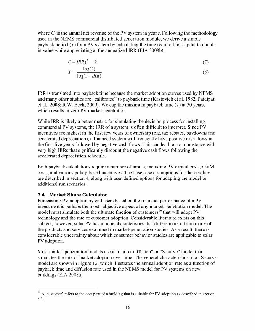
where Ct is the annual net revenue of the PV system in year t. Following the methodology used in the NEMS commercial distributed generation module, we derive a simple payback period (T) for a PV system by calculating the time required for capital to double in value while appreciating at the annualized IRR (EIA 2008b).

2)1( =+ TIRR (7)

)1log(

)2log(IRR

T+

= (8)

IRR is translated into payback time because the market adoption curves used by NEMS and many other studies are “calibrated” to payback time (Kastovich et al. 1982, Paidipati et al., 2008; R.W. Beck, 2009). We cap the maximum payback time (T) at 30 years, which results in zero PV market penetration.

While IRR is likely a better metric for simulating the decision process for installing commercial PV systems, the IRR of a system is often difficult to interpret. Since PV incentives are highest in the first few years of ownership (e.g. tax rebates, buydowns and accelerated depreciation), a financed system will frequently have positive cash flows in the first five years followed by negative cash flows. This can lead to a circumstance with very high IRRs that significantly discount the negative cash flows following the accelerated depreciation schedule.

Both payback calculations require a number of inputs, including PV capital costs, O&M costs, and various policy-based incentives. The base case assumptions for these values are described in section 4, along with user-defined options for adapting the model to additional run scenarios.

3.4 Market Share Calculator Forecasting PV adoption by end users based on the financial performance of a PV investment is perhaps the most subjective aspect of any market-penetration model. The model must simulate both the ultimate fraction of customers16

Most market-penetration models use a “market diffusion” or “S-curve” model that simulates the rate of market adoption over time. The general characteristics of an S-curve model are shown in Figure 12, which illustrates the annual adoption rate as a function of payback time and diffusion rate used in the NEMS model for PV systems on new buildings (EIA 2008a).

that will adopt PV technology and the rate of customer adoption. Considerable literature exists on this subject; however, solar PV has unique characteristics that differentiate it from many of the products and services examined in market-penetration studies. As a result, there is considerable uncertainty about which consumer behavior studies are applicable to solar PV adoption.

16 A ‘customer’ refers to the occupant of a building that is suitable for PV adoption as described in section 3.5.

17

Source: Adopted from LaCommare et al., 2003

Figure 12. Market share as a function of payback period used in NEMS

18

The curves in Figure 12 represent different payback periods, where products with a quicker payback time achieve a higher market share and have faster adoption rates. Market-penetration is simulated in the NEMS model by the product of the maximum market share and the adoption rate, expressed as follows:

PV Market Share(PV payback time, time) = Max Market Share(PV payback time) * Adoption Rate(time) (9)

SolarDS uses a similar dynamic market share calculator that is based on an S-Curve market diffusion model. PV market share is calculated by the product of the maximum market share (which is approximated using an empirical relationship to payback time) and the rate of adoption (which is approximated using a Bass diffusion model [Bass 1969, Mahajan, et al. 1990]). Figure 13 illustrates the computational steps in the market share module.

Figure 13. Computational steps involved in the market share module

SolarDS users have three options for characterizing the maximum market share as a function of payback time: (1) use the NEMS maximum market share curves (EIA 2004), (2) use the Navigant Consulting, Inc. curves (Paidipati et al. 2008), or (3) supply user-defined maximum market share curves. Each method has different maximum adoption curves to capture the different market dynamics for new and existing buildings. User-defined curves are calculated using an exponential fit (R.W. Beck 2009), defined as follows:

* e Payback Sensitivity Payback TimeMaximum Market Fraction −= (10)

19

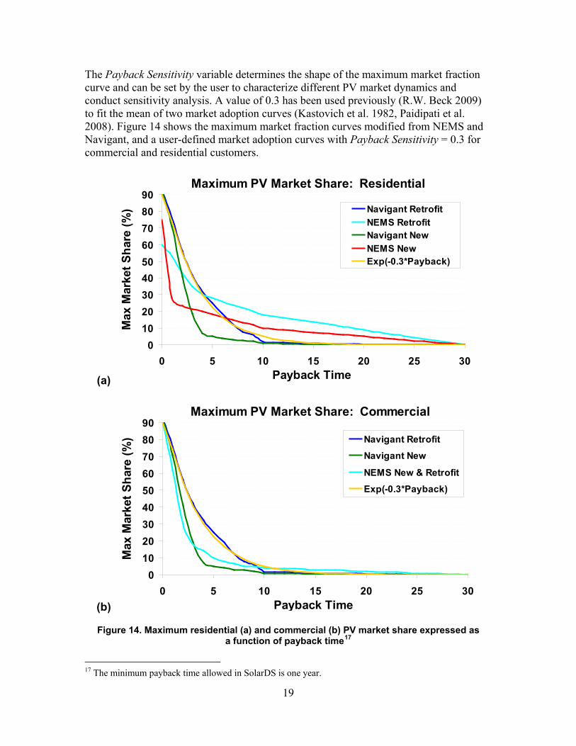
The Payback Sensitivity variable determines the shape of the maximum market fraction curve and can be set by the user to characterize different PV market dynamics and conduct sensitivity analysis. A value of 0.3 has been used previously (R.W. Beck 2009) to fit the mean of two market adoption curves (Kastovich et al. 1982, Paidipati et al. 2008). Figure 14 shows the maximum market fraction curves modified from NEMS and Navigant, and a user-defined market adoption curves with Payback Sensitivity = 0.3 for commercial and residential customers.

(a)

Maximum PV Market Share: Residential

0102030405060708090

0 5 10 15 20 25 30Payback Time

Max

Mar

ket S

hare

(%) Navigant Retrofit

NEMS RetrofitNavigant NewNEMS NewExp(-0.3*Payback)

(b)

Maximum PV Market Share: Commercial

0102030405060708090

0 5 10 15 20 25 30Payback Time

Max

Mar

ket S

hare

(%) Navigant Retrofit

Navigant New

NEMS New & Retrofit

Exp(-0.3*Payback)

Figure 14. Maximum residential (a) and commercial (b) PV market share expressed as a function of payback time17

17 The minimum payback time allowed in SolarDS is one year.

20

The rate of PV adoption (S-Curve) is calculated using the Bass-Diffusion model, expressed as follows:

Adoption Rate (t) = Tqp

Tqp

epqe

•+−

•+−

+

−

)(

)(

1

1 (11)

where T is the time from the initial year the product was introduced, p represents the “coefficient of innovation” characterizing early adopters of a technology, and q represents the “coefficient of imitation” characterizing late adopters of a technology. We simulate increasing adoption rates with decreasing payback times, as indicated by the three S-curves used in SolarDS that are shown in Figure 15. Additionally, users can modify the p and q parameters to simulate different PV diffusion rates.

Figure 15. PV adoption rates based on PV payback times and the amount of time PV has been in the market

One complication of using multiple S-curves is transitioning from one curve to another when PV payback periods decrease with PV cost reductions and/or increasing electricity rates. Since the market-penetration fraction scales the total building stock, this transition would lead to a step increase in PV adoption in the year that the model switched from one curve to another. To smooth this transition, we calculate the position on the new S-curve by solving for the “equivalent year” that represents the previous year’s market share, shown in Equation 12, which is equivalent to equation 11 solved for T using the previous year’s market share:

0%

20%

40%

60%

80%

100%

0 5 10 15 20 25 30

Years the Technology has been in the Market

Cum

ulat

ive

Ado

pter

s

payback < 3 years

3 < payback < 10 years

payback > 10 years

21

Max Market Share(t -1)1-Max Market Share(t)ln

Max Market Share(t -1) q1+ *Max Market Share(t) p

Equivalent Year =-(p+q)

(12)

After the equivalent year is calculated, the model steps forward in time by two years and solves for the total market share using the p and q parameters from the new S-curve. The initial year for the diffusion curves is set to 2001, when the total U.S. installations exceeded 25 MW. The initial year is set to 1999 in California to characterize the quicker adoption rates (Paidipati et al. 2008).

3.5 Calculating building stock and aggregating PV installations The market share calculator produces an array containing hundreds of thousands of PV purchasing probabilities that are unique to each building type, size, age, utility rate structure, and local solar insolation. To estimate the number of buildings that will have PV installed, PV adoption probabilities must be multiplied by the actual number of buildings corresponding to the combination of input parameters. The number of buildings is calculated in a building stock database that consists of multidimensional arrays that characterize the range of unique buildings types for residential and commercial buildings. This building stock database is populated from a variety of sources.

Residential Building Array The residential buildings stock for attached and detached single-family homes, mobile homes, and rental units is estimated from the 2000 U.S. Census. The fraction of each building type that is occupied by an owner or renter is estimated using the EIA’s 2005 Residential Energy Consumption Survey (RECS) (EIA 2005). The base building stock is scaled down to remove homes that are unsuitable for PV, primarily due to shading. Shading estimates are applied at the EIA’s “Census + 4” regions, which includes the census regions plus the four largest states. Data on shading are limited, and the base SolarDS case uses a previous national estimate that is adjusted to increase shading in the eastern United States and decrease shading in the Southwest. Shading fraction assumptions are listed in Appendix C.

The growth rate of residential building stock is forecasted in two-year increments from 2008 to 2030, based on census population projections at the state level. We assume that: (1) the building stock will grow in proportion to the state population, (2) the regional distribution of the population will stay fixed, and (3) the distribution of building types will remain constant.

After simulating the base number of homes suitable for PV, the building stock library categorizes these homes, based on the following seven array dimensions: SolarDS region, building size, roof orientation, finance type, rate type, rate bin, and building vintage.

1. SolarDS Region. Census data provide the numbers of detached single-family homes, attached single-family homes, and mobile homes in each state. The states

22

are then divided into SolarDS regions, based on census blocks. Each census block is assigned to a specific TMY meteorological site. The number of buildings in each SolarDS region is calculated from the fraction of the state population that resides in the associated census blocks.

2. Building PV Size. SolarDS calculates a range of residential PV system sizes based on building types, where the “average” size for a residential PV installation is 4.3 kW and 3.8 kW for new and existing detached single-family homes, 3.2 kW and 3.0 kW for new and existing attached single-family homes, and 2.0 kW for all mobile homes. The size distribution is assumed to be uniform in all geographical regions.

3. Roof Orientation. We assume a distribution of solar orientations in the SolarDS model. For residential homes, we assume that 10% of buildings have flat roofs and the remaining 90% have pitched roofs characterized by seven solar orientations that are uniformly distributed around 360°. Roof characteristics are assumed to be identical for all geographical regions. A table of roof orientations and distributions is provided in Appendix C.

4. Finance Type. SolarDS uses a distribution of down payment fractions and marginal tax rates to characterize the variety of financed residential PV systems (see Appendix D). Users can modify customer down payment fractions, marginal tax rates, loan rates, and loan terms to quantify the sensitivity of PV adoption to various scenarios.

5. Rate Type. SolarDS allows users to select from three rate types: all flat, all time-of-use (TOU), and a combination of flat and TOU rates that changes over time to reflect the gradual adoption of TOU rates. The “all flat” and “all TOU” options are provided to test the sensitivity of PV deployment using the two rate structure bounds.

6. Rate Bin. SolarDS splits residential customers into five rate bins in each region to characterize the distribution of customer rates, as discussed in section 2.2.

7. Vintage. The cost of PV installations on pre-existing buildings is higher than the cost of PV installations on new construction. SolarDS allows users to specify the relative cost reduction for new buildings, which in the reference case is set to 10%. New and existing buildings also use different maximum market-penetration curves, reflecting the different decision process made by the builder and homeowner. Existing buildings are calculated from the census data, as described above. New construction is primarily driven by the growth in building stock but also from rebuilds.

Rental properties represent a large fraction of commercial and residential buildings. This significantly limits the use of solar PV. Building owners, who do not pay the electric bill, have no incentive to install PV. Renters have limited incentive to make long-term capital investments on property they do not own. The fraction of homes that are rented for attached single-family, detached single-family, and mobile homes are 12%, 34%, and 17%, respectively, as taken from the 2001 Residential Energy Consumption Survey

23

(RECS) at the EIA’s “Census + 4” regions. PV adoption on rental units is simulated separately using decreased market-penetration curves that can be modified by the user.

Commercial Building Array Creation of the commercial building array begins with the “base” number of commercial buildings in the EIA’s 2003 Commercial Buildings Energy Consumption Survey (CBECS) (EIA 2003), allocated for the “Census + 4” regions. To account for roof shading, the amount of roof area is decreased by a regional shading fraction using a similar methodology as was used for residential buildings. Leased units are estimated using a uniform rent/own fraction for each region, based on the CBECS tax status in owned buildings (taxable/non-taxable). PV adoption on leased buildings is simulated using decreased market-penetration curves. This establishes the “base” number commercial buildings suitable for PV, which the building stock library then categorizes based on six array dimensions: SolarDS region, roof orientation, occupant class, building type, rate type, rate bin, and age.

1. SolarDS Region. Commercial buildings are allocated to SolarDS regions, based on the fraction of the state population in census blocks associated with TMY stations, as described previously.

2. Roof Orientation. Commercial PV orientations are based on the type on the “predominant roof material” of each building type, as reported in the CBECS database. If the reported roof material is shingle, wood, or slate, the roof is assumed to be pitched. For pitched roofs, we assume the same roof slope as residential buildings and the azimuth orientations listed in Appendix C. For the remaining roof types, we assume a flat roof surface filled with equal parts flat oriented PV and southerly facing PV, tilted at 25°. Fewer commercial roof orientations are evaluated than residential roof orientations because of the much larger size of the commercial building stock array.

3. Occupant Class. There are four classes of building occupants: for-profit owner occupied, non-profit owner occupied, leased, and government owned. These distinctions are made for three reasons. First, non-profit and government buildings are not taxable. Second, non-profit and government buildings may have a different decision-making process for evaluating PV investment. Finally, leased buildings likely have either a significantly lower market adoption rate or a third-party owner of the PV systems. Ownership data are derived from the CBECS tax status in owned buildings (taxable/non-taxable).

4. Building Type. SolarDS uses 14 building types from the Commercial Buildings Energy Consumption Survey database (EIA, 2003). Available roof area for PV is calculated by building type. PV installation sizes are calculated for each building type by scaling the available roof space by the module efficiency (W/ft2). The types of buildings and associated roof areas are listed in Appendix C.

5. Utility Rate Class. SolarDS allows users to select from four rate types: all flat rates, all time-of-use (TOU) rates, all demand-based rates, and mixed rates, which represent a combination of flat, TOU, and demand-based rates. The all flat, all

24

TOU, and all demand options are provided as benchmarks to test the sensitivity of PV adoption to commercial rate structures.

6. Vintage. As with residential buildings, users are given the option to set how much less expensive PV will be on new commercial buildings than on existing buildings. Also, new and existing buildings use different maximum market-penetration curves, reflecting the different decision-making processes followed by builders and owners. New and existing commercial building stock is calculated from census projections, similar to the way in which building stock is calculated for residential buildings.

Based on these assumptions, the total potential PV capacity (technical potential) in SolarDS by 2030 is 583 GW, including 271 GW of residential and 312 GW of commercial PV capacity, which is in line with previous estimates of U.S. rooftop PV capacity (Denholm and Margolis 2008). Using the Navigant Consulting maximum market-penetration curves, the maximum obtainable rooftop PV capacity18

Buildings Aggregator

by 2030 is 425 GW (182 GW residential, 243 GW commercial). Using the NEMS market-penetration curves, the maximum obtainable rooftop PV capacity by 2030 is 225 GW (95 GW residential, 130 GW commercial).

Once the residential and commercial buildings databases are established, the number of buildings adopting PV is calculated by multiplying the number of buildings in each class by the adoption fraction associated with each class. Figure 16 illustrates general approach for aggregating the new and existing buildings with PV. This process is run separately for residential and commercial buildings.

Figure 16. Aggregating buildings with PV

The submodule begins by calculating the existing building stock available for PV for each unique building type. The number of existing buildings with PV is calculated from

18 Minimum PV payback times are capped at one year in SolarDS due to model resolution.

Building Stock Aggregator

Initial building stock database

Existing Buildings Suitable for PV

New Buildings Suitable for PV

Home Rebuilds

No PV installed at the end of year

Existing Buildings with PV

Cumulative PV installations by State

Building growth projections database

25

the product of the fractional market share and the total number buildings in that particular building class.

The model similarly calculates the fraction of new buildings that install PV. The number of new buildings is calculated from the sum of (1) building growth calculated from census population projections at the state level, and (2) building rebuilds, which are assumed to be 1% of the existing buildings per year. The adoption of PV on new buildings is calculated from the product of the number of new buildings and the current adoption rate, calculated by the market share calculator. New buildings that do not adopt PV are then placed into the existing building stock.

The number of buildings with PV is summed over each building type to produce the amount of installed PV capacity (MW), and the fraction of buildings with PV for each state and time period. Total PV capacity (MW) is calculated from the product of the number of buildings that install PV and the size of the PV installation by building type. The state results are further aggregated to give national PV statistics for each time period.

4 SolarDS Results

SolarDS outputs the results of each simulation to a new Microsoft Excel workbook that includes user-defined run parameters saved in a main worksheet and the model output (at the state and national level) in a series of worksheets that include:

1. Annual PV Capacity

2. Cumulative PV Capacity

3. Annual Residential PV Capacity

4. Cumulative Residential PV Capacity

5. Annual Commercial PV Capacity

6. Cumulative Commercial PV Capacity

7. Annual # of Residential Buildings that Installed PV

8. Cumulative # of Residential Buildings that Installed PV

9. Annual # of Commercial Buildings that Installed PV

10. Cumulative # of Commercial Buildings that Installed PV

11. Fraction of Residential Buildings with PV

12. Fraction of Commercial Buildings with PV

13. Annual Cost of Residential Incentives

14. Annual Cost of Commercial Incentives

15. Cumulative Cost of Residential and Commercial Incentives

16. Residential Payback Times (aggregated to the state level)

17. Commercial Payback Times (aggregated to the state level)

26

The output file also contains an automated plotting tool to help the user quickly visualize SolarDS results.

4.1 SolarDS Example Results The amount of PV penetration simulated by SolarDS is highly dependent on model input parameters, primarily (1) future PV cost reductions, (2) the assumed maximum PV market-penetration curves as a function of PV financial performance, and (3) PV financing and policy-based assumptions. We illustrate the range of SolarDS output using six PV penetration scenarios. In the first four scenarios, we simulate PV adoption for combinations of high and low PV cost reductions and two maximum market share curves. In the last two scenarios, we illustrate the upper bound on PV penetration using high PV cost reductions in addition to aggressive financing and policy-based parameters. These parameters are defined by (1) decreasing the loan rate from 6% (real) to 4% (real), (2) increasing the loan term from 15 to 30 years for residential retrofit and commercial systems, (3) changing the residential loan structure so that 30% of customers pay no down payment on PV loans and 70% of customers pay a 20% down payment, (4) increasing the electricity rate escalations from AEO 2009 estimates to a 1% annual increase, and (5) adding a cost to future carbon emissions. The input parameters for the six model scenarios are summarized in Table 1.

27

Table 1. SolarDS Input Parameters Scenario ( PV Cost / Market-Penetration Curve / Finance & Policy )

EIA/ NEMS/ Base

EIA/ Navigant/

Base

DOE SETP/ NEMS/ Base

DOE SETP/

Navigant/ Base

DOE SETP/ NEMS/

Aggressive

DOE SETP/ Navigant/

Aggressive

PV Cost EIA EIA DOE-SETP

DOE-SETP

DOE-SETP DOE-SETP

Max PV Market Share

NEMS Navigant NEMS Navigant NEMS Navigant

Rate Escalation AEO 2009 AEO 2009 AEO 2009 AEO 2009 1% Annual 1% Annual Rate Structures Base Mix Base Mix Base Mix Base Mix Base Mix Base Mix

Carbon Pricea

-

-

-

-

$20/ton CO2 2010 - 2020 $30/ton CO2 2021 - 2030

$20/ton CO2 2010 - 2020 $30/ton CO2 2021-2030

Federal ITC 30% to 2016 com: 10% after

30% to 2016 com: 10% after

30% to 2016 com: 10% after

30% to 2016 com: 10% after

30% to 2016 res: 10% after com: 10% after

30% to 2016 res: 10% after com: 10% after

State Incentives Current Incentives

Current Incentives

Current Incentives

Current Incentives

Current Incentives

Current Incentives

Loan Rate 6% (real) 6% (real) 6% (real) 6% (real) 5% (real) 5% (real) Loan Term

(years) Com: 15b Resnew: 30 Resexisting: 15

Com: 15 Resnew: 30 Resexisting: 15





Down

Payment (%)

Com 20% 20% 20% 20% 20% 20% 20% of

Res Homes

100%

100%

100%

100%

0%

0%

80% of Res

Homes

20%

20%

20%

20%

20%

20%

a U.S. $2008 dollars b Bolinger (2009)

Simulated PV penetration is shown in Figures 17 through 19. It ranges from 15 to 193 GW of PV capacity installed by 2030. The amount of installed PV capacity is highly dependent on future PV cost reductions. Modeled cumulative installed PV capacity reaches approximately 12 GW if future cost reductions follow EIA estimates (PV reaches $4.23/W and $2.85/W by 2030 for residential and commercial systems). Simulated PV capacity is approximately five times higher if PV cost reductions follow the DOE SETP targets (PV reaches $2.09/W and $1.66/W for residential and commercial systems by 2030). PV penetration is also highly sensitive to financing parameters, where a combination of the attractive financing parameters and a cost associated with carbon emissions (summarized in Table 1) leads to 158-193 GW of PV capacity by 2030.

The different PV maximum adoption fractions based on PV financial performance (NEMS and Navigant, see Figure 14) lead to small differences in the lower penetration

28

scenarios, but significant differences (> 25 GW) in the high penetration scenario. This reflects similar adoption estimates for PV systems with higher payback times but a fundamental difference in estimated PV adoption for systems with very short payback periods. Additionally, the Navigant maximum market share curves lead to a significantly higher fraction of commercial to residential PV installations.

Cumulative Installed PV Capacity

0

25

50

75

100

125

150

175

200

2005 2010 2015 2020 2025 2030

PV C

apac

ity (G

W)


Figure 17. Cumulative installed PV capacity through 2030 for a range of model input

parameters, including PV costs (EIA and DOE SETP), PV market adoption rates (NEMS and Navigant), and PV financing and policy assumptions (base case and aggressive case)

Cumulative Residential PV Capacity

0

10

20

30

40

50

60

70

2005 2010 2015 2020 2025 2030

PV C

apac

ity (G

W)

PV Cost / Market Penetration / Finance & PolicyDOE SETP / Navigant / AggressiveDOE SETP / NEMS / AggressiveDOE SETP / NEMS / BaseDOE SETP / Navigant / BaseEIA / NEMS / BaseEIA / Navigant / Base

Figure 18. Cumulative installed residential PV capacity

29

Cumulative Commercial PV Capacity

0

20

40

60

80

100

120

140

2005 2010 2015 2020 2025 2030

PV C

apac

ity (G

W)


Figure 19. Cumulative installed commercial PV capacity

30

Table 2. Reference Case SolarDS Cumulative Installed PV Capacity

Scenario PV

Cost Market Share 2008 2010 2012 2014 2016 2018 2020 2022 2024 2026 2028 2030

Reference Casea

EIA

NEMS

Total 0.8 1.9 3.5 5.7 6.5 7.8 8.7 10.5 11.2 12.1 13.3 14.9 Residential 0.4 0.7 1.0 1.4 1.8 2.3 2.6 2.7 2.9 3.1 3.5 3.9 Commercial 0.4 1.2 2.5 4.3 4.8 5.5 6.1 7.8 8.3 9.0 9.8 10.9

EIA

Navigant


DOE SETP

NEMS


DOE SETP

Navigant


Attractive Caseb

DOE SETP

NEMS


DOE SETP

Navigant


a Reference case PV financing simulation, EIA electricity rate escalations, no carbon tax. b Attractive financing simulation, 1% annual electricity rate escalations and a $20-30/TonC cost for carbon emissions.

31

References

Ansar, J.; Sparks, R. (2009). “The Experience Curve, Option Value and the Energy Paradox.” Energy Policy (37); pp. 1012-1020. Bass, F.M. (1969). “A New Product Growth for Model Consumer Durables.” Management Science (18); pp. 215-227.

Boedecker, E.; Cymbalsky, J.; Wade, S. (2000). Modeling Distributed Electricity Generation in the NEMS Buildings Models. Washington, D.C.: EIA.

Bolinger, M. (2009). Financing Non-Residential Photovoltaics Projects: Options and Implications. LBNL-1410E. Berkeley, CA: Ernest Orlando Lawrence Berkeley National Laboratory. Denholm, P.; Margolis, R. M. (November 2008). Supply Curves for Solar PV-Generated Electricity for the United States. NREL/TP-670-44073. Golden, CO: National Renewable Energy Laboratory, 18 pp.

Denholm, P.; Margolis, R.; Milford, J. (2009). “Quantifying Avoided Fuel Use and Emissions from Solar Photovoltaic Generation in the Western United States.” Environ. Sci. Technol. (43); pp. 226-232.

DOE, U.S. Department of Energy (2008). Solar Energy Technologies Program: Multi Year Program Plan 2008-2012. Washington, DC: DOE, 125 pp.

Dutton, J.M.; Thomas, A. (1984). “Treating Progress Functions as a Managerial Opportunity.” Academy of Management Review (9:1); pp. 235-247.

Energy Information Administration (EIA), (2003). “Commercial Buildings Energy Consumption Survey.” http://www.eia.doe.gov/emeu/cbecs/. Accessed September 2009.

Energy Information Administration (EIA), (2004). The Electricity Market Module of the National Energy Modeling System: Model Documentation Report. DOE/EIA-M068(2004). Washington, DC: DOE, 253 pp.

Energy Information Administration (EIA), (2005). “Residential Energy Consumption Survey.” http://www.eia.doe.gov/emeu/recs/. Accessed September 2009.

Energy Information Administration (EIA), (2008a). Commercial Sector Demand Module of the National Energy Modeling System: Model Documentation 2008. DOE/EIA-M066(2008). Washington, DC: U.S. Department of Energy.

Energy Information Administration (EIA), (2008b). Model Documentation Report: Residential Sector Demand Module of the National Energy Modeling System. DOE/EIA-M067(2008). Washington, DC: U.S. Department of Energy.

http://www.eia.doe.gov/emeu/cbecs/�

32

Energy Information Administration (EIA), (2008c). Model Documentation: Renewable Fuels Module of the National Energy Modeling System. DOE/EIA-M069(2008). Washington, DC: U.S. Department of Energy.

Energy Information Administration (EIA), (2009a). Annual Energy Outlook 2009 with Projections to 2030. DOE/EIA-0383(2009). Washington, DC: U.S. Department of Energy.

Energy Information Administration (EIA), (2009b). State Energy Data System, www.eia.doe.gov/emeu/states/sep_sum/html/pdf/sum_pr_res.pdf. Accessed September 2009.

Fisher, J.C.; Pry, R.H. (1971). “A Simple Substitution Model of Technological Change.” Technological Forecasting and Social Change (3); pp. 75-88.

Fuller, M.C.; Portis, S.C.; Kammen, D.M. (2009). “Toward a Low-carbon Economy: Municipal Financing for Energy Efficiency and Solar Power.” Environment (January-February 2009).

Goldman, C.; Osborn J.; Hopper, N.; Singer, T. (2002). Market Trends in the U.S. ESCO Industry: Results from the NAESCO Database Project. LBNL-49601. Berkeley, CA: Ernest Orlando Lawrence Berkeley National Laboratory.

Griffith, B.; Long, N.; Torcellini, P.; Judkoff, R.; Crawley D.; Ryan J. (2008). Methodology for Modeling Building Energy Performance across the Commercial Sector. NREL/TP-550-41956. Golden, CO: National Renewable Energy Lab.

Hoff, T., Perez, R.; Margolis, R.M. (2007). “Maximizing the value of customer-sited PV systems using storage and controls.” Solar Energy (81:7); pp. 940-945.

Hoff, T.; Margolis, R.M. (2004). “Are Photovoltaic Systems Worth More to Residential Consumers on Net Metered Time-of-Use Rates?” Paper presented at the ASES 2004 Conference, July 11-14, 2004.

Jiang, Z.; Bass, F.M.; Bass, P.I. (2006). “Virtual Bass Model and the Left-hand Data-truncation Bias in Diffusion of Innovation Studies.” International Journal of Research in Marketing (23); pp. 93-106.

Kastovich, J.C.; Lawrence, R.R.; Hoffmann; Pavlak, C. (1982). Advanced Electric Heat Pump Market and Business Analysis. ORNL/Sub/79-2471/1. Prepared under subcontract for Oak Ridge National Laboratory by Westinghouse Electric Corp. Oak Ridge, TN: Oak Ridge National Laboratory.

LaCommare, K.H.; Edwards, J.L.; Marney, C. (2003). Distributed Generation Capabilities of the National Energy Modeling System (NEMS). LBNL-52432. Berkeley, CA: Ernest Orlando Lawrence Berkeley National Laboratory.

33

Mahajan, V.; Muller, E.; Bass, F.M. (1990). “New Product Diffusion Models in Marketing: A Review and Directions for Research.” Journal of Marketing (54); pp. 1-26.

Margolis, R.M.; Wood, F. (2004). “The Role for Solar in the Long-Term Outlook of Electric Power Generation in the U.S.” Paper presented at the 24th USAEE/IAEE North America Conference, Washington, DC, July, 8-10, 2004.

Marion, B.; Anderberg, M.; Gray-Hann, P. (November 2005). Recent Revisions to PVWATTS. NREL/CP-520-38975. Golden, CO: National Renewable Energy Laboratory.

Maycock, P.D. (2002). The World Photovoltaic Market. Report. Warrenton, VA: PV Energy Systems.

Mills, A.; Wiser, R.; Barbose, G.; Golove, W. (2008). “The Impact of Retail Rate Structures on the Economics of Commercial Photovoltaic Systems in California.” Energy Policy (36); pp. 3266-3277.

Nemet, G.F. (2006). “Beyond the Learning Curve: Factors Influencing Cost Reductions in Photovoltaics.” Energy Policy (34); pp. 3218-3232.

North Carolina Solar Center (2007). “Database of State Incentives for Renewables and Efficiency.” Raleigh, NC: North Carolina State University. http://www.dsireusa.org/. Accessed July 2009.

NREL (April 2007). National Solar Radiation Database1991-2005 Update: User’s Manual. NREL/TP-581-41364. Golden, CO: National Renewable Energy Laboratory.

Packey, D.J. (February 1993). Market Penetration of New Energy Technologies. NREL/TP- 462-4860. Golden, CO: National Renewable Energy Laboratory.

Paidipati, J.; Frantzis, L.; Sawyer, H.; Kurrasch, A. (February 2008). Rooftop Photovoltaics Market Penetration Scenarios. Subcontract Report NREL/SR-581-42306. Burlington, MA: Navigant Consulting, Inc.

R.W. Beck (January 2009). Distributed Renewable Energy Operating Impacts and Valuation Study. Prepared for Arizona Public Service by R.W. Beck, Inc.

Shama, A., ed. (1981). Marketing Solar Energy Innovations. New York: Praeger Scientific.

Short, W.; Packey, D.J.; Holt, T. (March 1995). A Manual for the Economic Evaluation of Energy Efficiency and Renewable Energy Technologies. NREL/TP-462-5173. Golden, CO: National Renewable Energy Laboratory.

Strategies Unlimited (March 2003). Photovoltaic Five-Year Market Forecast 2002-2007. Report PM-52. Mountain View, CA: Strategies Unlimited.

34

Wilcox, S.; Marion, W. ( May 2008). Users Manual for TMY3 Data Sets. NREL/TP-581-43156. Golden, CO: National Renewable Energy Laboratory.

Wiser, R.; Barbose, G.; Peterman, C. (February 2009). Tracking the Sun: The Installed Cost of Photovoltaics in the U.S. from 1998-2007. LBNL-1516E. Berkeley, CA: Lawrence Berkeley National Laboratory.

Wiser, R.; Bolinger, M.; Cappers, P.; Margolis, R. (2007). “Analyzing Historical Cost Trends in California’s Market for Customer-sited Photovoltaics.” Progr. Photovolt: Res. Appl. (15); pp. 69-85.

35

Bibliography

Canada Centre for Mineral and Energy Technology (CANMET), (1989). The Emerging Photovoltaic Industry: An Analysis of Literature on International Markets and Trends. Ottawa, Ont.: Peat Marwick Consulting Group. Farhar-Pilgrim, B.; Unseld, C.T. (1982). America’s Solar Potential: A National Consumer Study. New York: Praeger Scientific. Feldman, S.L.; Wirtshafter, R.M. (1980). On the Economics of Solar Energy: The Public Utility Interface. Lexington, MA: Lexington Books. Frantzis, L.; Friedman, D.; Hill, S.; Teagan, P. (1995). Building-Integrated Photovoltaics (BIPV): Analysis and U.S. Market Potential. Prepared for U.S. Department of Energy (DOE). No. 44513. Cambridge, MA: Arthur D. Little, Inc., 176 pp. Hamilton, B.; Shapiro, A. (April 1996). Market-Based Program Designs for Accelerated Implementation of Rooftop PV in New England. Report to the Boston Edison DSM Settlement Board. Burlington, VT: Vermont Energy Investment Corporation, 59pp. Iannucci, J.J.; Weinberg, C.J. (1991). A Diffusion Model for the Entry of Photovoltaics into Utilities, PG & E Research and Development Advanced Energy Systems Report 007.3-91.4, May 1991. San Ramon, CA: PG & E. Kendall, D.L.; Cates, S.C. (1991). Market Penetration of New Technologies, Programs and Services, Research Project 2864-1., Research Triangle Park, NC: Research Triangle Institute. Shama, A., ed. (1981). Marketing Solar Energy Innovations. New York: Praeger Scientific. Utility Photovoltaic Group (UPVG) (1994). Utility Planning for PV Systems, Part 3. Washington D.C.: Utility Photovoltaic Group.

36

Appendix A: Model Regions and Electricity Rates

Figure A-1. EIA Census + 4 Regions

Table A-1. SolarDS Electricity Price Regions

SolarDS Price Region

Representative Utility Residential Electricity Prices

Commercial Electricity Prices

Mean Min Max Mean Min Max Alabama Alabama Power Co 9.32 6.40 13.70 8.70 5.58 13.87 Arizona Arizona Public Service Co 9.66 5.31 13.19 8.27 2.05 12.06 Arkansas Entergy Arkansas Inc 8.73 5.43 12.59 6.91 4.10 10.73 California (North) Pacific Gas & Electric Co 14.41 8.40 23.42 13.23 6.11 14.21 California (South) Southern California Edison 14.41 5.88 24.21 11.86 2.55 21.44 Colorado Colorado Springs 9.25 6.06 13.80 7.62 2.24 18.55 Connecticut United Illuminating Co 19.08 11.68 20.62 13.60 10.81 17.42 Delaware Delmarva Power & Light Co. 13.15 10.78 15.70 10.59 8.55 15.29 District of Columbia Potomac Electric Power Co 11.15 11.16 14.26 9.72 10.98 14.01 Florida Florida Power Corp (Progress

Energy) 11.22 7.63 14.32 9.75 6.79 14.41

Georgia Georgia Power Co 9.10 5.47 13.63 8.07 5.79 12.50 Idaho Idaho Power Co 6.36 4.91 9.81 5.14 4.09 8.19 Illinois Commonwealth Edison Co 10.12 4.51 13.35 7.57 4.92 11.00 Indiana PSI Energy Inc (Cinergy) 8.26 4.80 10.98 7.29 4.21 20.71 Iowa Interstate Power (Alliant) 9.45 4.95 14.31 7.15 3.10 14.73 Kansas Kansas City Power & Light 8.19 4.85 14.42 6.84 2.74 34.12 Kentucky Kentucky Utilities Co 7.34 5.47 9.48 6.76 5.29 11.11 Louisiana Entergy Louisiana Inc 9.37 3.10 12.36 9.13 2.94 33.33 Maine Central Maine 9.62 9.37 34.64 8.27 9.23 23.82 Maryland Baltimore Gas & Electric Co 11.83 7.37 14.42 10.23 7.06 18.11 Massachusetts Boston Edison (Nstar) 15.53 9.21 18.65 12.56 10.06 19.87 Michigan Detroit Edison Co 10.21 6.21 18.31 8.69 6.38 17.01 Minnesota Northern States Power Co 9.18 5.36 14.58 7.48 1.88 13.59 Mississippi Entergy Mississippi Inc 9.36 7.22 12.01 8.92 6.94 12.70

37

Missouri Union Electric Co (Ameren) 7.69 4.67 13.48 6.34 3.96 13.52 Montana NorthWestern Energy LLC 8.77 4.67 11.16 8.18 1.57 10.58 Nebraska Omaha Public Power District 7.59 4.90 12.87 6.39 1.85 15.12 Nevada (North) Sierra Pacific Power Co 8.40 5.64 13.04 6.09 4.15 12.56 Nevada (South) Nevada Power Company 11.92 5.50 13.26 10.76 0.87 14.06 New Hampshire Public Service Co of NH 14.88 10.18 31.70 12.65 10.20 16.37 New Jersey Jersey Central Power & Lt Co 14.14 9.11 15.30 11.75 9.18 15.98 New Mexico Public Service Co of NM 9.12 7.59 16.65 7.66 3.86 41.97 New York (Long Island)

Long Island Power Authority 20.25 18.49 22.67 16.11 16.81 20.99

New York (NYC) Consolidated Edison-NYC 19.08 19.08 30.62 17.50 17.18 19.75 New York (Remain) Niagara Mohawk Power Corp 13.30 2.64 19.36 10.40 3.37 18.42 North Carolina Carolina Power & Light

(Progress) 9.40 6.70 13.86 7.43 5.94 16.67

North Dakota Northern States Power Co 7.30 4.93 9.73 6.58 1.90 9.32 Ohio Ohio Power Co (AEP) 9.35 5.56 12.85 8.22 4.71 13.24 Oklahoma Oklahoma Gas & Electric Co 8.58 5.37 16.40 7.33 4.48 28.99 Oregon Portland General Electric

Company 8.19 4.22 10.70 7.11 3.40 10.96

Pennsylvania PECO Energy Co 10.86 6.99 20.45 8.98 5.09 17.94 Rhode island Narragansett Electric Co 14.04 13.85 40.12 11.89 12.15 42.02 South Carolina South Carolina Electric & Gas 9.19 7.50 15.63 7.74 4.61 11.32 South Dakota Black Hills Power Inc 8.07 4.85 11.49 6.61 1.98 17.16 Tennessee Memphis City of 7.84 1.37 11.51 8.09 5.61 12.97 Texas TXU Energy Retail Co LP 12.34 7.32 18.16 9.87 4.10 16.24 Utah PacifiCorp 8.15 2.64 11.90 6.54 2.08 13.25 Vermont Central Vermont Pub Service 14.15 8.16 16.91 12.29 9.63 18.51 Virginia Virginia Electric & Power

(Dominion) 8.74 6.26 12.99 6.38 5.51 13.14

Washington Puget Sound Energy Inc 7.26 2.27 9.92 6.56 2.28 10.00 West Virginia Appalachian Power Co 6.73 6.15 13.15 5.85 5.58 13.20 Wisconsin Wisconsin Electric Power Co 10.87 6.17 15.45 8.71 5.65 13.87 Wyoming PacifiCorp 7.75 2.94 13.06 6.25 1.68 13.12

Because load patterns may vary for different climate patterns in northern and southern California, the state is separated into two regions to allow for different TOU rates. Nevada is split into two regions to allow for escalation based on the NEMS EMM regions. New York is separated into three regions. Generation and transmission into New York City and Long Island is severely constrained, resulting in much higher than average prices.

Table A-2. AEO 200919

Regiona

Rate Escalation by Region: Residential

2008 2010 2012 2014 2016 2018 2020 2022 2024 2026 2028 2030 % NE 1.00 0.93 0.97 0.97 0.97 0.98 0.99 0.98 0.99 1.01 1.02 1.03 0.1 MA 1.00 0.89 0.93 0.97 0.98 0.99 1.00 1.00 1.03 1.06 1.08 1.09 0.7

ENC 1.00 0.95 0.97 0.99 1.00 1.01 1.02 1.04 1.05 1.08 1.10 1.12 0.5 WNC 1.00 1.01 1.02 1.03 1.02 1.02 1.02 1.02 1.02 1.03 1.04 1.06 0.3 SA 1.00 0.96 0.99 1.00 1.01 1.02 1.03 1.04 1.06 1.10 1.13 1.14 0.8

ESC 1.00 0.98 0.98 0.98 0.98 0.99 0.99 1.00 1.02 1.05 1.08 1.10 0.8 WSC 1.00 0.93 0.95 0.97 0.98 1.00 1.03 1.04 1.06 1.10 1.13 1.14 0.7 MTN 1.00 1.02 1.02 1.03 1.05 1.09 1.11 1.12 1.17 1.22 1.26 1.30 1.4 PAC 1.00 0.96 0.94 0.93 0.93 0.94 0.94 0.94 0.95 0.98 1.00 1.01 0.1

a Regions are shown in Figure A-1.

19 Real, not nominal, electricity rate escalations (EIA 2009).

38

Table A-3. AEO 2009 Rate Escalation by Region: Commercial

Regiona 2008 2010 2012 2014 2016 2018 2020 2022 2024 2026 2028 2030 % NE 1.00 0.89 0.89 0.87 0.87 0.89 0.91 0.90 0.92 0.94 0.97 0.99 -0.1 MA 1.00 0.85 0.86 0.89 0.92 0.94 0.95 0.96 0.99 1.03 1.06 1.08 0.6 ENC 1.00 0.92 0.91 0.91 0.93 0.95 0.97 0.99 1.00 1.04 1.07 1.10 0.7 WNC 1.00 0.99 0.99 1.00 0.99 1.00 1.00 0.99 1.00 1.01 1.03 1.06 0.8 SA 1.00 0.92 0.94 0.94 0.94 0.95 0.96 0.96 0.98 1.02 1.05 1.06 0.7 ESC 1.00 0.95 0.94 0.92 0.92 0.93 0.93 0.94 0.96 0.99 1.02 1.04 0.3 WSC 1.00 0.90 0.90 0.92 0.92 0.96 0.99 1.00 1.03 1.08 1.12 1.14 0.5 MTN 1.00 0.97 0.94 0.93 0.94 0.97 0.98 0.98 1.02 1.06 1.10 1.13 0.9 PAC 1.00 0.97 0.92 0.89 0.89 0.90 0.90 0.89 0.90 0.93 0.95 0.97 -0.1 a Regions are shown in Figure A-1.

Table A-4. SolarDS Regions and Population Allocation

SolarDS Site Number

SolarDS Electricity

Rate Region

TMY Site (State & City)

Allocated Population (yr 2000)

Fraction of State

Population 1 AL AL Birmingham 1,572,515 35.36% 2 AL AL Huntsville 907,369 20.40% 3 AL AL Montgomery 759,750 17.08% 4 AL AL Mobile 620,977 13.96% 5 AL GA Columbus 302,428 6.80% 6 AL MS Meridian 102,777 2.31%

7 AL TN Chattanooga 97,596 2.19%

8 AL FL Tallahassee 69,559 1.56% 9 AL GA Atlanta 14,129 0.32%

10 AR AR Little Rock 1,329,509 49.73% 11 AR AR Fort Smith 628,182 23.50% 12 AR TN Memphis 395,581 14.80% 13 AR LA Shreveport 170,909 6.39% 14 AR MO Springfield 139,097 5.20% 15 AR MS Jackson 10,122 0.38% 16 AZ AZ Phoenix 3,275,528 63.84% 17 AZ AZ Tucson 1,094,445 21.33% 18 AZ AZ Flagstaff 296,989 5.79% 19 AZ AZ Prescott 179,906 3.51% 20 AZ NV Las Vegas 140,581 2.74% 21 AZ CA San Diego 122,405 2.39% 22 AZ UT Cedar City 9,379 0.18%

23 AZ NM Albuquerque 7,672 0.15%

24 AZ CO Grand Junction 3,727 0.07%

25 CA So CA Long Beach 8,706,405 25.70%

26 CA No CA San Francisco 7,101,835 20.97%

27 CA So CA Los Angeles 6,245,807 18.44%

28 CA No CA Sacramento 3,859,322 11.39% 29 CA So CA San Diego 3,285,362 9.70% 30 CA So CA Fresno 1,568,991 4.63% 31 CA So CA Daggett 1,103,365 3.26% 32 CA So CA Bakersfield 750,676 2.22% 33 CA So CA Santa Maria 658,686 1.94% 34 CA No CA Arcata 348,186 1.03% 35 CA No NV Reno 136,149 0.40% 36 CA No OR Medford 74,816 0.22% 37 CA So AZ Prescott 14,411 0.04% 38 CA So NV Tonopah 7,501 0.02%

39

39 CA So NV Las Vegas 7,002 0.02% 40 CA No OR Burns 1,594 0.00% 41 CA So AZ Phoenix 1,540 0.00% 42 CO CO Boulder 2,773,036 64.47%

43 CO CO Colorado Springs 667,357 15.52%

44 CO CO Grand Junction 251,827 5.85%

45 CO CO Pueblo 205,112 4.77% 46 CO CO Eagle 178,849 4.16% 47 CO CO Alamosa 87,957 2.04% 48 CO WY Cheyenne 65,940 1.53% 49 CO KS Goodland 46,235 1.07% 50 CO NE Scottsbluff 23,387 0.54% 51 CT CT Bridgeport 1,681,647 49.38% 52 CT CT Hartford 1,415,748 41.57% 53 CT RI Providence 204,546 6.01% 54 CT MA Worchester 54,689 1.61%

55 CT NY New York City 48,935 1.44%

56 DC VA Sterling 308,382 53.91% 57 DC MD Baltimore 263,677 46.09% 58 DE DE Wilmington 715,639 91.33% 59 DE NJ Atlantic City 65,930 8.41% 60 DE PA Philadelphia 2,031 0.26% 61 FL FL Tampa 4,380,438 27.41% 62 FL FL Miami 3,871,126 24.22%

63 FL FL Daytona Beach 2,863,036 17.91%

64 FL FL West Palm Beach 2,004,991 12.55%

65 FL FL Jacksonville 1,493,393 9.34% 66 FL FL Tallahassee 677,509 4.24% 67 FL AL Mobile 526,559 3.29% 68 FL AL Montgomery 89,085 0.56% 69 FL FL Key West 76,241 0.48% 70 GA GA Atlanta 4,094,795 50.02% 71 GA GA Macon 824,151 10.07% 72 GA GA Athens 754,462 9.22% 73 GA GA Savannah 545,545 6.66%

74 GA TN Chattanooga 455,212 5.56%

75 GA GA Columbus 435,625 5.32% 76 GA GA Augusta 430,861 5.26% 77 GA FL Tallahassee 386,233 4.72% 78 GA FL Jacksonville 223,874 2.73% 79 GA TN Knoxville 30,782 0.38% 80 GA NC Asheville 4,913 0.06% 81 KS IA Des Moines 879,236 30.05% 82 KS IL Moline 654,336 22.36% 83 KS IA Waterloo 603,638 20.63% 84 KS IA Sioux City 252,352 8.62% 85 KS IA Mason City 226,679 7.75% 86 KS NE Omaha 213,387 7.29% 87 KS WI La Crosse 43,869 1.50% 88 KS SD Sioux Falls 37,013 1.26% 89 KS MN Rochester 14,291 0.49%

90 KS MO Kansas City 1,523 0.05%

91 ID ID Boise 584,342 45.16% 92 ID ID Pocatello 425,334 32.87% 93 ID WA Spokane 267,814 20.70%

40

94 ID MT Missoula 14,240 1.10% 95 ID NV Elko 1,297 0.10% 96 IL IL Chicago 7,930,677 63.86% 97 IL IL Springfield 886,011 7.13% 98 IL MO St. Louis 872,763 7.03% 99 IL IL Rockford 793,140 6.39%

100 IL IL Peoria 696,099 5.60% 101 IL IN Evansville 384,252 3.09% 102 IL IL Moline 380,800 3.07% 103 IL WI Milwaukee 325,274 2.62% 104 IL IN Indianapolis 92,878 0.75% 105 IL MO Columbia 55,277 0.45% 106 IL WI Madison 2,122 0.02% 107 IN IN Indianapolis 2,563,710 42.16% 108 IN IN Fort Wayne 939,718 15.45% 109 IN IN South Bend 811,154 13.34% 110 IN IL Chicago 639,617 10.52% 111 IN IN Evansville 484,918 7.97% 112 IN KY Louisville 383,808 6.31% 113 IN KY Covington 176,230 2.90% 114 IN OH Dayton 81,330 1.34% 115 KS KS Wichita 854,287 31.78%

116 KS MO Kansas City 742,639 27.62%

117 KS KS Topeka 602,412 22.41% 118 KS KS Dodge City 247,028 9.19% 119 KS OK Tulsa 85,965 3.20% 120 KS MO Springfield 60,854 2.26%

121 KS NE Grand Island 44,366 1.65%

122 KS KS Goodland 42,533 1.58% 123 KS NE North Platte 5,953 0.22% 124 KS TX Amarillo 2,381 0.09% 125 KY KY Louisville 1,179,255 29.18% 126 KY KY Lexington 1,024,225 25.34% 127 KY IN Evansville 521,506 12.90% 128 KY KY Covington 401,353 9.93% 129 KY WV Huntington 343,734 8.50% 130 KY TN Nashville 295,411 7.31% 131 KY TN Bristol 138,437 3.43% 132 KY TN Knoxville 123,850 3.06% 133 KY TN Memphis 13,046 0.32%

134 LA LA New Orleans 1,650,111 36.92%

135 LA LA Baton Rouge 1,342,161 30.03%

136 LA LA Shreveport 789,351 17.66%

137 LA LA Lake Charles 581,675 13.02%

138 LA MS Jackson 101,030 2.26% 139 LA TX Port Arthur 2,323 0.05% 140 LA TX Lufkin 1,241 0.03% 141 LA AR Little Rock 1,084 0.02% 142 MA MA Boston 3,942,239 62.09% 143 MA MA Worchester 942,773 14.85% 144 MA RI Providence 681,104 10.73% 145 MA CT Hartford 667,208 10.51% 146 MA NY Albany 112,944 1.78% 147 MA NH Concord 2,829 0.04% 148 MD MD Baltimore 3,812,860 71.99% 149 MD VA Sterling 1,074,159 20.28% 150 MD DE Wilmington 225,657 4.26%

41

151 MD WV Elkins 101,035 1.91% 152 MD NJ Atlantic City 33,529 0.63% 153 MD VA Norfolk 24,184 0.46% 154 MD PA Harrisburg 22,844 0.43% 155 MD VA Richmond 2,218 0.04% 156 ME ME Portland 1,106,971 86.83% 157 ME ME Caribou 161,071 12.63% 158 ME NH Concord 6,879 0.54% 159 MI MI Detroit 4,119,864 41.45% 160 MI MI Flint 1,521,185 15.31%

161 MI MI Grand Rapids 1,268,740 12.77%

162 MI MI Lansing 916,640 9.22% 163 MI MI Muskegon 466,710 4.70% 164 MI OH Toledo 403,237 4.06%

165 MI MI Traverse City 402,807 4.05%

166 MI IN South Bend 312,555 3.14% 167 MI MI Alpena 161,440 1.62% 168 MI MI Houghton 159,262 1.60%

169 MI MI Sault Ste. Marie 83,312 0.84%

170 MI WI Green Bay 82,885 0.83% 171 MI IN Fort Wayne 39,807 0.40%

172 MN MN Minneapolis 2,925,313 59.46%

173 MN MN Saint Cloud 750,930 15.26% 174 MN MN Rochester 290,122 5.90% 175 MN ND Fargo 277,098 5.63% 176 MN MN Duluth 275,310 5.60% 177 MN SD Sioux Falls 128,968 2.62% 178 MN MN Int. Falls 102,273 2.08% 179 MN IA Mason City 100,571 2.04% 180 MN WI La Crosse 66,761 1.36% 181 MN MI Houghton 2,133 0.04% 182 MO MO St. Louis 2,305,473 41.20%

183 MO MO Kansas City 1,339,611 23.94%

184 MO MO Springfield 928,348 16.59% 185 MO MO Columbia 789,478 14.11% 186 MO TN Memphis 183,023 3.27% 187 MO IA Des Moines 25,526 0.46% 188 MO NE Omaha 7,522 0.13% 189 MO IL Moline 6,541 0.12% 190 MO AR Fort Smith 5,576 0.10% 191 MO AR Little Rock 3,290 0.06% 192 MS MS Jackson 987,829 34.73% 193 MS TN Memphis 640,766 22.53% 194 MS MS Meridian 566,672 19.92% 195 MS AL Mobile 392,699 13.80%

196 MS LA Baton Rouge 107,514 3.78%

197 MS LA New Orleans 106,861 3.76%

198 MS AL Huntsville 35,500 1.25% 199 MS AL Birmingham 4,255 0.15% 200 MS AR Little Rock 2,562 0.09% 201 MT MT Helena 215,795 23.92% 202 MT MT Billings 160,099 17.75% 203 MT MT Missoula 156,726 17.37% 204 MT MT Kalispell 114,474 12.69% 205 MT MT Great Falls 92,603 10.26%

42

206 MT MT Lewistown 48,210 5.34% 207 MT MT Miles City 46,451 5.15% 208 MT MT Glasgow 30,864 3.42% 209 MT MT Cut Bank 26,874 2.98% 210 MT WY Sheridan 9,725 1.08% 211 NC NC Raleigh 2,415,001 30.00% 212 NC NC Charlotte 1,937,866 24.07% 213 NC NC Greensboro 1,565,781 19.45% 214 NC NC Wilmington 968,937 12.04% 215 NC NC Asheville 553,844 6.88% 216 NC VA Norfolk 186,361 2.32% 217 NC TN Bristol 117,225 1.46%

218 NC NC Cape Hatteras 99,890 1.24%

219 NC SC Greenville 77,647 0.96% 220 NC TN Knoxville 72,009 0.89% 221 NC VA Richmond 54,752 0.68% 222 ND ND Fargo 299,370 46.62% 223 ND ND Bismarck 169,768 26.44% 224 ND ND Minot 161,314 25.12% 225 ND SD Rapid City 5,255 0.82% 226 ND SD Huron 3,288 0.51% 227 ND MT Miles City 3,205 0.50% 228 NE NE Omaha 1,003,230 58.63%

229 NE NE Grand Island 255,129 14.91%

230 NE NE Norfolk 170,039 9.94% 231 NE NE North Platte 123,185 7.20% 232 NE NE Scottsbluff 87,861 5.13% 233 NE IA Sioux City 44,784 2.62% 234 NE KS Topeka 14,250 0.83% 235 NE SD Pierre 4,749 0.28% 236 NE KS Goodland 3,696 0.22% 237 NE SD Rapid City 3,378 0.20% 238 NH NH Concord 1,036,495 83.87% 239 NH MA Boston 90,888 7.35% 240 NH MA Worchester 67,484 5.46% 241 NH ME Portland 40,919 3.31% 242 NJ NJ Newark 4,737,665 56.30% 243 NJ PA Philadelphia 1,393,310 16.56%

244 NJ NY New York City 1,183,079 14.06%

245 NJ NJ Atlantic City 802,935 9.54% 246 NJ PA Allentown 218,664 2.60% 247 NJ DE Wilmington 78,697 0.94%

248 NM NM Albuquerque 1,160,120 63.78%

249 NM TX El Paso 330,045 18.14% 250 NM NM Tucumcari 150,391 8.27% 251 NM TX Midland 88,442 4.86% 252 NM CO Alamosa 53,246 2.93%

253 NM CO Grand Junction 22,789 1.25%

254 NM CO Pueblo 7,509 0.41% 255 NM AZ Tucson 4,324 0.24% 256 NM TX Lubbock 2,180 0.12% 257 NV South NV Las Vegas 1,402,358 70.18% 258 NV North NV Reno 498,607 24.95% 259 NV North NV Elko 46,363 2.32%

260 NV North NV Winnemucca 29,454 1.47%

261 NV North NV Ely 10,799 0.54%

43

262 NV North NV Tonopah 8,231 0.41% 263 NV North UT Cedar City 2,445 0.12%

264 NYC NY New York City 10,444,179 55.04%

265 NY Long Is. CT Bridgeport 1,609,017 8.48% 266 NY Remain NY Albany 1,363,859 7.19% 267 NY Remain NY Buffalo 1,301,957 6.86% 268 NY Remain NY Syracuse 1,194,945 6.30% 269 NY Remain NY Rochester 1,167,876 6.15% 270 NY Remain NJ Newark 683,302 3.60% 271 NY Remain NY Binghamton 600,670 3.17% 272 NY Remain NY Massena 177,545 0.94% 273 NY Remain PA Bradford 162,687 0.86% 274 NY Remain VT Burlington 123,234 0.65% 275 NY Remain PA Williamsport 65,309 0.34%

276 NY Remain PA Wilkes-Barre 43,752 0.23%

277 NY Remain PA Erie 30,434 0.16% 278 NY Long Is. RI Providence 7,253 0.04% 279 OH OH Cleveland 2,081,112 18.33% 280 OH OH Columbus 1,971,782 17.37% 281 OH OH Dayton 1,575,838 13.88% 282 OH OH Akron 1,430,359 12.60% 283 OH KY Covington 1,401,769 12.35% 284 OH OH Toledo 950,637 8.37%

285 OH OH Youngstown 706,904 6.23%

286 OH OH Mansfield 584,256 5.15% 287 OH WV Huntington 264,509 2.33% 288 OH PA Pittsburgh 187,418 1.65% 289 OH WV Charleston 89,023 0.78% 290 OH IN Fort Wayne 86,071 0.76% 291 OH PA Erie 22,699 0.20%

292 OK OK Oklahoma City 1,532,614 44.42%

293 OK OK Tulsa 1,205,649 34.94%

294 OK TX Wichita Falls 258,003 7.48%

295 OK AR Fort Smith 245,796 7.12% 296 OK TX Fort Worth 79,327 2.30% 297 OK KS Wichita 64,081 1.86% 298 OK KS Dodge City 39,340 1.14% 299 OK TX Amarillo 22,345 0.65% 300 OK MO Springfield 2,625 0.08% 301 OR OR Portland 1,496,864 43.75% 302 OR OR Salem 600,743 17.56% 303 OR OR Eugene 416,059 12.16% 304 OR OR Medford 339,927 9.94% 305 OR OR Redmond 165,561 4.84% 306 OR OR Pendleton 129,504 3.79% 307 OR OR North Bend 124,757 3.65% 308 OR OR Astoria 63,423 1.85% 309 OR ID Boise 33,681 0.98% 310 OR OR Burns 19,947 0.58% 311 OR WA Yakima 19,267 0.56% 312 OR CA Arcata 11,269 0.33% 313 PA PA Philadelphia 3,234,722 26.34% 314 PA PA Pittsburgh 2,725,698 22.19% 315 PA PA Harrisburg 1,770,423 14.42% 316 PA PA Allentown 1,447,170 11.78%

317 PA PA Wilkes-Barre 763,011 6.21%

44

318 PA PA Williamsport 566,515 4.61% 319 PA PA Bradford 524,237 4.27% 320 PA DE Wilmington 429,600 3.50% 321 PA PA Erie 417,499 3.40%

322 PA OH Youngstown 207,952 1.69%

323 PA VA Sterling 87,401 0.71% 324 PA NY Binghamton 67,329 0.55% 325 PA WV Elkins 27,144 0.22% 326 PA MD Baltimore 6,507 0.05% 327 PA NJ Newark 5,846 0.05% 328 RI RI Providence 1,043,056 99.50% 329 RI MA Worchester 5,263 0.50% 330 SC SC Greenville 1,146,765 28.58% 331 SC SC Columbia 989,877 24.67% 332 SC SC Charleston 895,614 22.32% 333 SC NC Charlotte 340,746 8.49% 334 SC GA Augusta 205,513 5.12% 335 SC NC Wilmington 203,937 5.08% 336 SC GA Savannah 161,436 4.02% 337 SC GA Athens 40,482 1.01% 338 SC NC Asheville 17,608 0.44% 339 SC NC Raleigh 9,391 0.23% 340 SD SD Sioux Falls 261,762 34.68% 341 SD SD Rapid City 180,019 23.85% 342 SD SD Huron 170,861 22.64% 343 SD SD Pierre 74,640 9.89% 344 SD NE Norfolk 23,383 3.10% 345 SD IA Sioux City 21,031 2.79% 346 SD ND Fargo 14,552 1.93% 347 SD ND Bismarck 8,596 1.14% 348 TN TN Nashville 1,838,670 32.32% 349 TN TN Memphis 1,388,930 24.41% 350 TN TN Knoxville 1,085,595 19.08%

351 TN TN Chattanooga 691,610 12.16%

352 TN TN Bristol 486,175 8.55% 353 TN AL Huntsville 186,174 3.27% 354 TN NC Asheville 12,129 0.21% 355 TX TX Fort Worth 5,608,872 26.90% 356 TX TX Houston 4,955,756 23.77% 357 TX TX San Antonio 1,916,970 9.19% 358 TX TX Austin 1,434,729 6.88% 359 TX TX Brownsville 978,369 4.69%

360 TX TX Corpus Christi 750,132 3.60%

361 TX TX Waco 748,004 3.59% 362 TX TX El Paso 690,669 3.31% 363 TX TX Lufkin 637,769 3.06% 364 TX LA Shreveport 494,013 2.37% 365 TX TX Port Arthur 431,235 2.07% 366 TX TX Midland 390,808 1.87% 367 TX TX Lubbock 389,346 1.87% 368 TX TX Amarillo 382,332 1.83% 369 TX TX Abilene 309,567 1.48% 370 TX TX Victoria 273,952 1.31%

371 TX TX Wichita Falls 224,372 1.08%

372 TX TX San Angelo 208,457 1.00% 373 TX NM Tucumcari 12,779 0.06%

374 TX LA Lake Charles 6,917 0.03%

45

375 TX AR Fort Smith 3,715 0.02% 376 TX KS Dodge City 3,057 0.01%

377 UT UT Salt Lake City 1,999,247 89.53%

378 UT UT Cedar City 167,106 7.48%

379 UT WY Rock Springs 34,848 1.56%

380 UT CO Grand Junction 27,207 1.22%

381 UT ID Pocatello 2,774 0.12% 382 UT NV Ely 1,503 0.07% 383 VA VA Sterling 2,331,222 32.93% 384 VA VA Norfolk 1,596,461 22.55% 385 VA VA Richmond 1,298,552 18.34% 386 VA VA Lynchburg 686,010 9.69% 387 VA VA Roanoke 598,542 8.46% 388 VA TN Bristol 308,708 4.36% 389 VA NC Greensboro 114,750 1.62% 390 VA WV Elkins 100,092 1.41% 391 VA NC Raleigh 26,430 0.37% 392 VA WV Charleston 14,425 0.20% 393 VA TN Knoxville 3,323 0.05% 394 VT VT Burlington 469,834 77.17% 395 VT NH Concord 60,899 10.00% 396 VT NY Albany 49,152 8.07% 397 VT MA Worchester 16,013 2.63% 398 VT CT Hartford 12,929 2.12% 399 WA WA Seattle 3,616,970 61.37% 400 WA WA Spokane 572,474 9.71% 401 WA WA Yakima 476,574 8.09% 402 WA OR Portland 440,819 7.48% 403 WA WA Olympia 427,598 7.25% 404 WA OR Pendleton 253,513 4.30% 405 WA OR Astoria 63,216 1.07% 406 WA WA Quillayute 42,957 0.73% 407 WI WI Milwaukee 1,981,735 36.95% 408 WI WI Green Bay 1,203,284 22.43% 409 WI WI Madison 997,047 18.59% 410 WI WI Eau Claire 446,623 8.33% 411 WI WI La Crosse 297,580 5.55% 412 WI IL Rockford 157,144 2.93%

413 WI MN Minneapolis 117,746 2.20%

414 WI MN Duluth 96,387 1.80% 415 WI MI Houghton 46,879 0.87% 416 WI IL Moline 11,857 0.22% 417 WI MN Rochester 6,733 0.13% 418 WV WV Charleston 778,188 43.03% 419 WV WV Elkins 450,975 24.94% 420 WV WV Huntington 190,247 10.52% 421 WV PA Pittsburgh 166,590 9.21% 422 WV VA Sterling 147,523 8.16% 423 WV VA Roanoke 69,468 3.84% 424 WV TN Bristol 5,353 0.30% 425 WY WY Cheyenne 122,428 24.79% 426 WY WY Casper 94,348 19.11% 427 WY WY Sheridan 76,994 15.59% 428 WY WY Lander 52,669 10.67%

429 WY WY Rock Springs 49,670 10.06%

430 WY MT Billings 29,315 5.94% 431 WY ID Pocatello 25,100 5.08%

46

432 WY NE Scottsbluff 14,945 3.03%

433 WY UT Salt Lake City 14,695 2.98%

434 WY SD Rapid City 12,531 2.54% 435 WY CO Eagle 1,087 0.22%

47

Appendix B: PV Performance and Cost Reductions Table B-1. PV Derate Factor by Component

Component Derate Factor PV module nameplate DC rating 0.95 Inverter and transformer 0.92 Mismatch 0.98 Diodes and connections 0.995 DC wiring 0.98 AC wiring 0.99 Soiling 0.95 System availability 0.98 Overall DC-to-AC derate Factor 0.77a

a This corresponds to the derate factor of a new module. We also assume that PV output degrades over time, resulting in a 10% reduction in 20 years.

Table B-2. PV Cost Reductionsa

Year

Residential ($/kW)

Commercial ($/kW)

EIA DOE - SPT EIA DOE - SPT PV Inverterb PV Inverter PV Inverter PV Inverter

2008 8000 729 8000 500 6800 527 6800 500 2010 6603 729 5159 310 5515 519 4128 200 2012 6438 729 4458 290 5024 519 3389 190 2014 6214 721 3756 280 4533 512 2650 180 2016 5704 717 3303 260 4192 512 2212 170 2018 5403 713 3099 240 4000 508 2075 160 2020 5101 709 2894 220 3808 504 1938 165 2022 4928 705 2721 210 3616 501 1861 150 2024 4754 705 2547 200 3424 497 1783 140 2026 4580 697 2386 190 3232 497 1727 130 2028 4406 693 2239 190 3040 493 1692 130 2030 4233 689 2091 190 2848 489 1657 130

a In nominal 2008 U.S. dollars b Inverter replacement is scheduled every 10-20 years, with inverter lifetime increasing over time.

Learning-based Cost Reductions The idea of learning-based cost reductions stems from the observation that workers in manufacturing plants become more efficient as they produce more units. This idea has been extended to describe the cost reductions and quality improvements in a wide variety of manufactured products. One reason for its widespread use is the availability of data on unit production and unit cost. The learning rate, LR, is derived from cost data, Ct, and cumulative manufactured data, qt, using the following relationship:

ln(1 )ln(2)

11

tLR

tt t

t

qC Cq

−

++

=

(B-1)

48

The global cumulative installed PV amount/rate is inferred from the cumulative amount of PV installed in a given time period using the fraction of PV installed in the US, fUS,t, as follows:

,

,

US tt

US t

qq

f= (B-2)

Recent surveys of PV learning rates suggest values ranging from 17% to 26% (Maycock 2002; Strategies Unlimited 2003; Nemet 2006). The NEMS model uses a constant PV learning rate of approximately 13%. SolarDS allows users to specify both the learning rate and the fraction of U.S. to global cumulative installed PV capacity for each time period in SolarDS. Figure B-1 shows the PV cost reductions for fixed learning rates of 17% and 26%, assuming a fixed U.S. to global cumulative installed PV capacity fraction.

Relative Cost of PV

0

0.2

0.4

0.6

0.8

1

0 10 20 30 40 50

Installed PV (GW)

Rela

tive

Cost

LR = 0.26 (Maycock, 2002) LR = 0.17 (Strat. Unlim, 2003) Figure B-1. PV Cost reductions for two PV learning rates (LR) derived in recent studies.

Although PV prices can be reasonably expected to decrease with cumulative production, users should keep certain factors in mind when using learning rates. Extrapolating learning rates from historical PV price and production data may not reflect the current and future reductions in PV costs. Additionally, learning rates are based on the cumulative global PV market, of which the U.S. share has declined steadily from more than 30% in the mid-1990s to 11% in 2006. SolarDS does not forecast the global PV market, and the user must specify the U.S. fraction of the global PV market from 2008 to 2030.

49

Appendix C: Building Assumptions

Table C-1. Residential Roof Orientations

Orientation

Tilt

Azimuth

Flat

4-sided Roof

2-sided Roof

Rooftop Fraction 10% 45% 45%

1 0° 0° 100% - - 10% 2 25° -90° - - 14% 6% 3 25° -60° - - 14% 6% 4 25° -30° - 33% 14% 21% 5 25° 0° - 33% 14% 21% 6 25° 30° - 33% 14% 21% 7 25° 60° - - 14% 6% 8 25° 90° - - 14% 6%

Table C-2. Regional Roof Shading

Region (EIA Census + 4) Shaded Fraction (%) California 35 East North Central 55 East South Central 55 Florida 35 Mid Atlantic 55 Mountain 40 New England 60 New York 55 Pacific 40 South Atlantic 55 Texas 35 West North Central 45 West South Central 55

Table C-3. Commercial Roof Orientations

Orientation Tilt Azimuth Rooftop Fractiona

1 0° 0° 10-50% 2 25° 0° 40-50% 3 25° -30° 0-25% 4 25° 30° 0-25%

a Commercial roof orientation fractions vary by building type within the range specified.

50

Table C-4. Commercial PV Capacity by Building Typea

Building Type

Roof Area (1000

ft2/building)

Unshaded

Fraction (%)

Potential Roof Capacity

( kW / building ) Education 15.59 80 112 Food Sales 4.88 80 35 Food Service 4.10 80 30 Inpatient 46.00 80 331 Outpatient 6.28 80 45 Lodging 12.65 80 91 Retail (other than mall) 7.66 80 55 Enclosed and Strip Malls 26.90 80 194 Office 6.02 80 43 Public Assembly 8.69 80 63 Public Order and Safety 9.20 80 66 Religious Worship 6.32 80 45 Service 5.35 80 38 Warehouse and Storage 13.79 80 99

a Represents unshaded commercial PV capacity by building type. This capacity is further reduced by the regional shading assumptions in Table C.2.

51

Appendix D: PV Financing Assumptions

The residential and commercial financing parameters are user input options in the SolarDS model. The reference case financing assumptions and the distribution of residential financing options are given below.

Table D-1. Residential Financing Inputs

Financing Parameters New Construction Retrofit Construction Loan Rate 6.0% (real) 6.0% (real) Loan Term 30 years 15 years

Table D-2. Distribution of Residential Financing

Down Payment Fraction Tax Rate Fraction of Households 20% 25% 40% 20% 33% 40% 100% 25% 10% 100% 33% 10%

Table D-3. Commercial Financing Parameters

Commercial Inputs Value Loan Term 15 years Loan Rate 6.0% (real) Down Payment Fraction 20% IRR analysis period 25 years

Table D-4. Commercial Capital Depreciation Schedule (MACRS)

Year Depreciation Fraction 1 20.00% 2 32.00% 3 19.20% 4 11.52% 5 11.52% 6 5.76%

52

Appendix E: PV Market-Penetration Curves

NEMS The maximum annual adoption of PV by residential and commercial customers is calculated in NEMS as follows (EIA 2008a, 2008b):

0.30 0.75, ( )New ConstructionMaximum Penetration Min

Payback Time years=

(E-1)

Existing Buildings0.30 0.005,

40* ( )Maximum Penetration Min

Payback Time years=

(E-2)

Navigant, Inc. The maximum PV market share from Navigant (Paidipati et al. 2008) was based on a customer survey of the potential residential adoption of a theoretical heat pump technology that is 20% more efficient than existing technology (Kastovich et al. 1982). The heat pump curve was decreased slightly, based on industry interviews. The Navigant study decreased the adoption rate on new construction for payback periods greater than three years because builders may be hesitant to include a technology with longer payback periods. Navigant curves result in significantly higher PV penetration than result from using NEMS curves for shorter payback periods.

R.W. Beck, Inc. The maximum PV market share from R.W. Beck (2009) was calculated using an exponential increase in PV adoption with decreasing payback time:

0.3* ( ) Payback Time years

All BuildingsMaximum Penetration e−= (E-3)

This parameterization approximates the mean between the maximum PV market share curves assumed in the Navigant study and the original Kastovich et al. (1982) curve.

F1147-E(10/2008)

REPORT DOCUMENTATION PAGE Form Approved OMB No. 0704-0188

The public reporting burden for this collection of information is estimated to average 1 hour per response, including the time for reviewing instructions, searching existing data sources, gathering and maintaining the data needed, and completing and reviewing the collection of information. Send comments regarding this burden estimate or any other aspect of this collection of information, including suggestions for reducing the burden, to Department of Defense, Executive Services and Communications Directorate (0704-0188). Respondents should be aware that notwithstanding any other provision of law, no person shall be subject to any penalty for failing to comply with a collection of information if it does not display a currently valid OMB control number. PLEASE DO NOT RETURN YOUR FORM TO THE ABOVE ORGANIZATION. 1. REPORT DATE (DD-MM-YYYY)

September 2009 2. REPORT TYPE

Technical Report 3. DATES COVERED (From - To)

4. TITLE AND SUBTITLE

The Solar Deployment System (SolarDS) Model: Documentation and Sample Results

5a. CONTRACT NUMBER DE-AC36-08-GO28308

5b. GRANT NUMBER

5c. PROGRAM ELEMENT NUMBER

6. AUTHOR(S) P. Denholm, E. Drury, and R. Margolis

5d. PROJECT NUMBER NREL/TP-6A2-45832

5e. TASK NUMBER PVD9.1210

5f. WORK UNIT NUMBER

7. PERFORMING ORGANIZATION NAME(S) AND ADDRESS(ES) National Renewable Energy Laboratory 1617 Cole Blvd. Golden, CO 80401-3393

8. PERFORMING ORGANIZATION REPORT NUMBER NREL/TP-6A2-45832

9. SPONSORING/MONITORING AGENCY NAME(S) AND ADDRESS(ES)

10. SPONSOR/MONITOR'S ACRONYM(S) NREL

11. SPONSORING/MONITORING AGENCY REPORT NUMBER

12. DISTRIBUTION AVAILABILITY STATEMENT National Technical Information Service U.S. Department of Commerce 5285 Port Royal Road Springfield, VA 22161

13. SUPPLEMENTARY NOTES

14. ABSTRACT (Maximum 200 Words) The Solar Deployment System (SolarDS) model is a bottom-up, market-penetration model that simulates the potential adoption of photovoltaics (PV) on residential and commercial rooftops in the continental United States through 2030. NREL developed SolarDS to examine the market competitiveness of PV based on regional solar resources, capital costs, electricity prices, utility rate structures, and federal and local incentives. This report provices details on the model, which uses the projected financial performance of PV systems to simulate PV adoption for building types and regions then aggregates adoption to state and national levels. The main components of SolarDS include a PV performance simulator, a PV annual revenue calculator, a PV financial performance calculator, a PV market share calculator, and a regional aggregator. The model simulates a variety of installed PV capacity for a range of user-specified input parameters. PV market-penetration levels from 15 to 193 GW by 2030 were simulated in preliminary model runs. SolarDS results are primarily driven by three model assumptions: (1) future PV cost reductions, (2) the maximum PV market share assumed for systems with given financial performance, and (3) PV financing parameters and policy-driven assumptions, such as the possible future cost of carbon emissions.

15. SUBJECT TERMS SolarDS; photovoltaics; PV; PV capacity; PV systems; solar deployment system; adoption; residential; commercial; buildings; state; national; United States; model; model results; market model; market penetration; market competitiveness; regional solar resources; solar capital costs; electricity prices; utility rate structures; federal incentives; local incentives; annual revenue; financial performance calculator; market share; cost reductions; financing parameters

16. SECURITY CLASSIFICATION OF: 17. LIMITATION OF ABSTRACT

UL

18. NUMBER OF PAGES

19a. NAME OF RESPONSIBLE PERSON a. REPORT

Unclassified b. ABSTRACT Unclassified

c. THIS PAGE Unclassified 19b. TELEPHONE NUMBER (Include area code)

Standard Form 298 (Rev. 8/98) Prescribed by ANSI Std. Z39.18

the solar deployment system technical report report nrel/tp-6a2-45832 september 2009 the solar...

Documents