the solubility of spin-polarized 3

Journal of Low Temperature Physics, Vol. 100, Nos. 3/4, 1995

The Solubility of Spin-Polarized 3He in 4He and the Superfluidity of 3He in 3He-4He Mixtures

Lars P. Roobol,* Giorgio Frossati, Kevin S. Bedell, t and Alexander E. Meyerovich:~

Kamerlingh Onnes Laboratorium, Rijksuniversiteit Leiden, P.O. Box 9506, NL-2300 RA, Leiden, The Netherlands

(Received September 26, 1994; revised March 20, 1995)

We investigate the possibility of a large enhancement of the T = 0 finite solubility of 3He in 4He due to spin-polarization. The size of the effect depends on the fraction of SHe atoms in the system. We present two different approaches for the limits of a small and a large number of 3He atoms compared to the number of 4He atoms. Since the possible 3He superfluid phase transition depends' on 3He density, we calculate the consequences of this change in the solubility for its superfluid transition temperature. It is shown that for small fi'actions of SHe, the transition temperature is enhanced mostly due to the enlargement of the up-spin Fermi sphere. In the opposite limit the transition temperature is enhanced as a result of the increased 3He solubility. PACS: 67.60.Fp, 64.75. + g, 67.75. + z

1. INTRODUCTION

A superfluid transition of the 3He sub-system in 3He-4He mixtures remains one of the most intriguing problems of low-temperature physics, as it would provide us with a unique mixture of two distinct superfluids. At present, not only the transition temperature and its dependence on thermodynamic variables like pressure are unknown, but even the exact type of pairing and the symmetry of the order parameter are unclear. As a result, theoretical estimates for T c differ by several orders of magnitude. Nevertheless, all theories agree on the point that the properties of this mixture of superfluids should be very different from those of pure 3He or 4He. This can justify the considerable experimental effort necessary to try to observe the 3He superfluid transition in 3He-erie mixtures.

*Now at: RoyaI Holloway, University of London, Egham, Surrey, TW20 0EX, U.K. tLos Alamos National laboratory - T 11, MS-B262, Los Alamos, NM 87545, U.S.A. ;Department of Physics, University of Rhode Island - Kingston, RI 02881, U.S.A.

339

0022-2291/95/0800-0339507.50/0 �9 1995 Plenum Publishing Corporation

340 L.P. Rooboi et aL

Up until now, some laboratories have cooled mixtures of various concentrations down to temperatures of 0.1-0.2 mK, 1-5 but none of them suc- ceeded in observing the 3He superfluid transition in mixtures. Because of a large number of experimental parameters (temperature T, pressure P, 3He concentration X and magnetic field B) it is necessary to investigate in which region of this parameter space one is most likely to observe this superfluid transition.

We argue that one of the best strategies, from both the theoretical and experimental point of view, is to study 3He-4He mixtures with a relatively high degree of spin-polarization of the 3He component. Recent achievements in the methods of spin polarization 6-1~ can make such an approach feasible.

As we will see, spin polarization can lead to considerable changes in either the limiting solubility of 3He in 4He or the effective (3He-) interaction, depending on the model chosen. Since the transition temperature depends on these quantities exponentially, the effect of spin polarization on the transition temperature can be rather dramatic.

As examples, we will consider the relevanl effects in the frames of both the s-wave and the potential models. In some sense, these models are opposite to each other: the s-wave model uses an unrenormalized interaction and relates all the polarization changes to the change in density of states, while the main effect for the potential models is the change in effective interaction. Therefore, the s-wave model predicts large changes in solubility with polarization which causes the transition temperature to increase exponentially. On the other hand, the solubility changes for the potential models are less significant than the exponential dependence of the transition temperature on renormalized interaction. Despite these major differences between the models, both predict that spin polarization could cause a very significant increase in transition temperature. The fact that both these opposite models predict a large increase in Tc signals that the study of spin-polarized mixtures can be very promising.

As an example of the behaviour of a potential model, we will use the one originally proposed by Bardeen. Baym and Pines, 11 extended to finite polarization by van de Haar, Bedell and Frossati 12 for calculating the properties of the mixture. The corresponding properties of the pure phase are calculated using the "nearly metamagnetic model" put forward by Bedell and Sanchez-Castro 13 using the (3He-~ fit parameters of Sanchez Castro, Bedell and Wiegers. ~4 We were able to solve the equations for phase equilibrium in the case where the volume of the mixture is much larger than that of the pure phase. In the opposite case~ we were able to solve them using the dilute gas model.

In the next section, we briefly review the results on finite solubility m

The Solubility of Spin-Polarized 3He in 4He 341

zero magnetic field, extending it to finite field in Sec. III, using several different approaches. In Sec. IV we discuss the consequences for the transition temperature. It is shown that a possibly large enhancement of the solubility of spin-polarized 3He in 4He and the corresponding increase in density of states has a much larger effect on Tc than the increase in pairing interaction.

2. SOLUBILITY AT ZERO MAGNETIC FIELD

Below 0.8 K, one cannot mix 3He and 4He in arbitrary proportions: above a certain limiting concentration x,(T) of 3He, the mixture decom- poses, as first observed by Walters and Fairbank, is into dilute 3He-4He mixtures (dilute phase) and practically pure 3He (concentrated phase).

While the 3He-rich mixtures are self purifying (their 4He solubility limit becomes vanishingly small upon approaching zero temperature16'17 ), the dilute mixtures have a finite solubility 18 even at T= O.

In this paper, we consider a fixed volume V containing a phase separated mixture at T = 0 consisting of N4 4He atoms with N34 3He atoms dissolved, and N 3 atoms in the concentrated phase. We define the total 3He concentration X and the 3He concentration x ~< X in the mixture as

N 3 -~ N34 X - (la)

N3 .~_ N34 Af_ N4

N34 x (lb)

N34 -k N 4

2.1. The Chemical Potentials

In thermodynamic equilibrium, the 3He. chemical potentials of both phases must be equal, i.e.,

/[~3(n3, P3) ~]A34(///34, P34,///4) (2)

where n 3 (n34) is the 3He density in the pure (dilute) phase, n 4 is the 4He density in the mixture and P is the pressure. Letting the pressure on both sides be equal fixes the density n,(P) at which Eq. (2) is satisfied.

In a fixed volume V, the chemical potentials are linked through the Gibbs-Duhem equations

dP3 = n3 dlz3 (3a)

dP34 = n34 d/~34 -Jr- H e dlu 4 (3b)

342 L . P . Roobol et aL

The last equation can be simplified for low 3He concentration using d/a 4 ~dP/n~ with n o the density of pure 4He. The 3He chemical potential of the mixture contains three terms,

p2 l"/34 = e 0 ( ~ 4 ) -}- {- 'gint(/'14, ///34) ( 4 )

2m*(kt4)

where e 0 is a constant depending on the 4He chemical potential #4 (or pressure), the second term is the Fermi energy of a gas of free particles with mass m*, and Fermi momentum p F = h k F = h(37~2/~34) 1/3. Finally, eint is a term due to the interaction between the 3He particles. This interaction term can be approximated by various methods. We will compare the results of three of such methods:

1. A fit to experimental data of Seligman etal. , 19"2~ compiled in Ref. 21. Here it was assumed that the chemical potential can be expanded in the 3He density as

-L. ~ ~2/3 .~ r~5/3 //'/34 = CO - - ~1'~34 q- c 2 n 3 4 -}- ~3'~34 ~- ~ (5)

Since this approach also fits the two lowest order terms of expansion (4) in n34 , we do not have to use assumptions for the values of e o and m*.

2. The s-wave approximation, a microscopic approach in which the energy spectrum is calculated using perturbation theory. At all concentrations up to the demixing line, mixtures form a system of slowly moving quasi-particles with the interaction rapidly decreasing at large distances. In this limit, the scattering of quasi-particles reduces effectively to s-wave scattering. 22'23 Then all the interaction processes can be described using only one parameter, namely the s-wave scattering length a 0. The value of a 0 has to be obtained experimentally. For 3He-4He mixtures, the interaction between 3He quasi-particles is effectively attractive, so the s-wave scattering length is negative, ao= 0.088nm. 24 The interaction term of Eq. (4) is given by 25

F4 (6) eint = ~ kN 2 + 4 (11 - 2 ln(2)) )~2 + " j

1/3 is assumed to be where the dimensionless parameter ,)~=peao/=h oc n34 small, which is equivalent to the condition n34~ [ao1-3, and the single- particle impurity effective mass mi is defined as

m i = lim m * ( ~ 3 4 ) ( 7 ) ~ 3 4 ~ 0


while the effective mass caused by quasi particle interactions is

m* 8 - - = 1 + 2 2 ( 7 1 n 2 - 1 ) + - . . (8) mi

3. The local effective potential model of Bardeen, Baym and Pines, I1 where it is assumed that the quasi-particle interaction can be described by an effective potential veff(~7) = Vo cos(q/ks), where k~ is the effective range of the potential with strength v 0. The lowest Legendre moments of the scattering amplitudes were calculated by van de Haar, Frossati and Bedel112 (hereafter referred to as HFB) in the thermodynamic limit. (1) An attempt to obtain better agreement with experiment was made by defining ks(n34 ) =k~(1 .-~-flH34/l/ls), with fl a dimensionless parameter allowing for a stronger dependence of veff on/'/34. With the interaction parameters we can obtain the Fermi liquid interaction parameter f p S =f}~ ' + ~cr'fpi', with I p l = I p ' l = PF. The moments o f f H enter the expression for gin t at T= 0 as follows, 26

f ~ s dgP ' ~int = 2 (f~F)[pl=P~(27~h)3

= v o n 3 4 ( 1 + ] 1-cos(2K)K 4

3 cos(2K) sin(2K) + 2 K ~ - + 3 ~ - + . . . ) (9)

.1/3 In this approach, m* is defined as where K = kF/k s = pF/hks oc "o34"

m* F~ - 1 + - - ( 1 0 )

m i 3

where the Landau parameter F~ can be calculated from the scattering amplitude a~ given in Ref. 12.

In principle, similar calculations can be done using other model representations for the effective potential (see, e.g., reviews25'27).

~Note a misprint just after their equation 24 d):

Sx = sin(2K) and Cx = cos(2K)

344 L. P. Roobol et aL

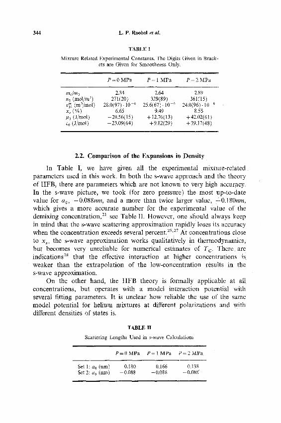
TABLE I

Mixture Related Experimental Constants. The Digits Given in Brack- ets are Given for Smoothness Only.

P = 0 MPa P = 1 MPa P = 2 MPa

mi/m 3 2.34 2.64 2.89 n 3 (mol/m 3) 271(20) 329(89) 361(15) v~4 (m3/mol) 28.0(97). 10 -6 25.6(67). 10 .6 24.0(96). 10 6 x~ (%) 6.65 9.49 8.55 /z 3 (J/mol) -20.56(15) +12.76(13) +42:02(61) eo (J/mol) -23.09(64) +9.82(29) +39.17(48)

2.2. Comparison of the Expansions in Density

In Table I, we have given all the experimental mixtm'e-related parameters used in this work. In bo th the s-wave approach and the theory of HFB, there are parameters which are not known to very high accuracy. In the s-wave picture, we took (for zero pressure) the most up-to-date value for ao, 0.088nm, and a more than twice larger value, -0 .180nm. which gives a more accurate number for the experimental value of the demixing concentrat ion, 21 see Table II. However. one should always keep in mind that the s-wave scattering approximat ion rapidly loses its accuracy when the concentrat ion exceeds several percent. 2s'27 At concentrat ions close to x, , the s-wave approximat ion works qualitatively in thermodynamics , but becomes very unreliable for numerical estimates of T c. There are indications 28 that the effective interaction at higher concentrat ions is weaker than the extrapolat ion of the low-concentrat ion results in the s-wave approximation.

On the other hand, the H F B theory is formally applicable at all concentrat ions, but operates with a model interaction potential with several fitting parameters. It is unclear how reliable the use of the same model potential for helium mixtures at different polarizations and with different densities of states is.

TABLE II

Scattering Lengths Used in s-wave Calculations

P=OMPa P = I M P a P=2MPa

Set 1: a o (nm) -0.180 -0.166 -0.138 Set 2: ao (nm) -0.088 -0.088 -0.088

The Solubility of Spin-Polarized 3He in 4He

TABLE II I

HFB Model Fit Parameters

P = 0 MPa P = 1 MPa P = 2 MPa

v0 (Jm 3) -1 .39 .10 -51 -1 .10 .10 -51 -0 .96 .10 -51 ks (m -1) 4.0.109 4.4.109 5.8.109 /~ 0.0 0.5 0.7

345

Instead of comparing malay different interaction potentials, we decided only to show results on one particular set of parameters for one particular potential, namely the one given by HFB, with the parameters given in Table III. This set of parameters is essentially the fit made by HFB to magnetostriction data,12 with the range parameter k~ adjusted to reproduce the experimental value of the solubility limit. Using the original fits of HFB did not change our results for x~ by more than 5 %.

It is instructive to compare the different expansions of the chemical potential as a function of the density. The experimental data and the HFB- expansion show the same functional dependence of/_t34 on F/34 , Eq. (5). The s-wave picture gives rise to an additional term proportional to n34-4/3. In Table IV, we compare the different terms for P = 0 MPa. The model of HFB is in good agreement with the experimental fit. The lowest order terms of the s-wave approach, especially for ao = -0 .088 nm, also agree with the experimental data. Because the functional dependence on //34 is different, it is better to compare the chemical potentials graphically, see Fig. 1, where we plotted chemical potential curves at P = 1 MPa for several models.

The steepest curve is the one for a Fermi gas without any interaction, which is equivalent to taking the a0 ---, 0 limit in the s-wave model or taking the Vo ~ 0 limit in the HFB model. At concentrations up to a few percent, the Fermi gas model and the s-wave model with ao = -0 .088 nm fit the

TABLE IV

Comparison Between Different Expansions of the Chemical Potential of 3He in Mixture #34 (J/tool) at P = 0 MPa in the 3He Density n34

(10 6 mol/m 3)

O2 n 2/3 o2 n o2 n 4/3 o2 n 5/3

experimental 194.6 -201 0 - 1.04.104 s-wave, ao = -0.18 nm 194.4 --387 1110 not listed s-wave, a o = --0.088 nm 194.4 - 189 266 not listed HFB model 181.9 - 2 3 4 0 -1 .10.104

346 L . P . R o o b o l et al.

4 - - - ao = - 0 " 0 8 8 nm j -

Fermi gas

3 e x p e r i m e n t J

HFB mode l j - - - J

o 2 ......... a 0 = - 0 . 1 6 6 n m / / - / f

~" 1 - / / " J -"~ ....................... v ~_ "" / .... :z~ 22-- J f

0 1 . . . . . . !

-2 / / " :

- 3 ! J ' ' r I , , . , I 4 , , ~ I , r r , I , ~ i

0 5 10 15 20 25

x(%) F i g . 1. T h e d i f f e r e n c e i n 3He c h e m i c a l p o t e n t i a l b e t w e e n p u r e 3 H e a n d 3He i n 3 H e - 4 H e

m i x t u r e s a s f u n c t i o n o f c o n c e n t r a t i o n a t P = 1 M P a . F u l l l i n e : e x p e r i m e n t a l c u r v e , d o t t e d l i n e :

s - w a v e a p p r o x i m a t i o n w i t h a 0 = - 0 . 0 8 8 n m , d a s h - d o u b l y d o t t e d l i n e : f r ee F e r m i g a s , d o t t e d

l i n e : s - w a v e a p p r o x i m a t i o n w i t h a 0 = - 0 . 1 6 6 n m , d a s h - d o t t e d l i n e : H F B m o d e l .

experimental data best, while the other curves lie below experiment. At higher concentrations, up until 15 %, deviations are smallest for the HFB model and the s-wave model with a 0 = -0 .166 nm, while the ones mentioned before keep on increasing steeply. This behaviour is seen at all pressures.

At concentrations higher than x~, the HFB curve is less steep than the s-wave curves. This means that in the s-wave picture it is more difficult to increase the concentration, because the energy needed to do so is higher.

The experimental data are extrapolated from 25 700 m K to T = 0 I see Ref. 21, and references therein). This means it is also possible to plot the chemical potential of mixtures of concentration above the T = 0 solubility limit (xs(T) = x~(0)(1 + flrT2)), up to X = 16 %. As we will see in Sec. IIIE. the solubility limit can be as high as 25%; theoretical curves lose their accuracy when extrapolated to such high concentrations.

Recent analysis 28 of experimental data 29'3~ on spin dynamics in 3He- 4He mixtures provides an additional confirmation that the effective attraction between 3He particles at high concentration is strongly suppressed m comparison with data at low concentration.


3. SOLUBILITY IN FINITE MAGNETIC FIELD

3.1. The Relative Amount of 3He

In a magnetic field B, the total system, the concentrated phase and the dilute mixture will have polarizations A, A 3 and A34, respectively, where

A - N3A3 + N34A34 (1 la) N3 + N34

N ~ - N ~ A, U~+U~ ( l ib)

Here ]" (+) stands for spin-up (down) particles and the index i is either "3" or "34". The relation between polarization and magnetic field is given by the susceptibility

8m 8A X =/A0 ~-~ =/20/A3Nn ~ (12)

where/10 = 4~. 10 7 j/(Am 2) is the magnetic permeability of the vacuum, /~3x = 0.778 mK/T the 3He nuclear magnetic moment and n is the number density of 3He particles. The susceptibility has only been measured in ther- mal equilibrium at low field; in the pure phase the measurements have been done by Ramm etal. ~L'32 and in mixtures by Ahonen etal. 33 Using the rapid melting technique, the susceptibility of pure 3He along the (depressed) melting curve has been measured by Wiegers, Wolff and Puech, 34 for polarizations up to A = 0.6. Otherwise, we have to estimate the susceptibility theoretically.

There is a distinct difference between polarization obtained in thermodynamic equilibrium by applying a large external field (the so-called brute force technique) and polarization determined by the history of the system, as in rapid melting experiments. This non-equilibrium polarization can be very long-lived, 7'8'35'36 and the evolution of the system, in this case, takes place at constant total polarization A, Eq. (lla). This imposes an additional constraint on the thermodynamic variables A3 and A34. In such a situation, one should describe the distribution of the 3He particles and polarization between the pure and dilute phase as a function of overall polarization A, the total number of 3He particles in the system, N = N3 + N34 and the total number of 4He particles N4. As a result, the solubility limit x, at T = 0 and the polarizations A 3 and A34 of both phases depend on A, N and N4. Then the corresponding value of xs(A, N, N4) dif- fers from the thermodynamic equilibrium value xs(A34, N34/N4) which does

348 L.P. Roobol et al.

not depend on N / N 4 . Therefore, one should carefully specify the experimental conditions under which the system demixes into a pure and a dilute phase.

In a magnetic field, the Gibbs-Duhem relations, Eqs. (3) change to

dP3 =//3 d/z3 + m3 dB (13a)

dP34 =//34 d,t-t 34 q- t/4 d//4 + m34 dB (13b)

where m =/z3NnA is the magnetization and B the magnetic field. Although Eqs. (13) are coupled by the condition dP3=dP34 in order to keep the pressure equal in both subsystems, many parameters can change in reac- tion to a change in, say, the external magnetic field.

A possible simplification is to restrict oneself to certain limits of X. For example, in the limit of X ~ 1, when most of the system is in the pure phase and the amount of mixture is very small, the presence of the dilute phase with polarization A34 and concentration x, practically does not affect the volume of the pure phase, nor its polarization A 3 ~, A, which is constant. Then the polarization A34 and the 3He density n34 depend only on A 3. The calculation of xs(A3) for these conditions is performed in Sec. IIIB. The opposite case, leading to a different solubility, corresponds to a system with a small amount of pure phase. In this case A34 ~ A is constant, and the polarization A 3 is a function of A34 while xs depends only on A34 and is not sensitive to A 3 .

Another possible approach is to reduce the number of parameters by demanding that certain boundary conditions must be met. In Sec. ItlC for example, we restrict ourselves to the case where d#4 = 0 and dP 3 = dP34 = O. Both approaches limit themselves to specific experimental arrangements, which makes it a priori difficult to compare them to each other.

3.2. XT1

The polarization dependence of the chemical potential #34 was calculated by Bashkin and Meyerovich 25 in the s-approximation using second order perturbation theory. In general, if the total polarization of the system is constant, the chemical potentials of the 3He Fermi liquids in the pure and dilute phases at T= 0 can be written as

(37"C2//3) 2/3 /A3(//3, A) - (1 + o'A) 2/3

2m* ~(A, n3)

(3~2n34) 2/3 /A~4(n34, A) = -e0(A,/~4, n34) -t-

2m*4,a(A, H4~ /734)

(14a)

(t +~rA) 2/3 (i4b)


If we assume, as was suggested in the previous Section, that the amount of 4He in the system is very small and the system consists mostly of pure 3He, X ~ 1, A3~A, we can equate /z~(A) and /z3~4(A) without having to use further equations for the polarizations. Restricting ourselves to the simplest realistic approximation in which eo is a constant and the effective masses do not depend on the signs of their spins, we get

I (Xs2(0)) 2/3 1 2/3 x,(A) = • +~2/3 (15a)

/1 V/3 / m 4(A) m].(0/] ~ = \ 2 n3v~') _(l +aA)Z/3m*(A) m*(0)j (15b)

where x = 19atn34, with ~)atn34, with v~ = 1/(n34 -}- 174) the average volume per atom in the mixture. This approximation is quite accurate for mixtures of not very high concentration; the error caused by the assumption rn~ -~ rn~' is unknown and should be higher than the error caused by the assumption eo = constant.

3.3. XJ, xs Imposing the conditions d#4=0 and dP=O on Eqs. (13) gives us the

simple relation 1

d/~i= -/13N Ai dB (16)

where i s { 3, 34}. Integrating this at constant density ni gives

B /ti(ni, B)-/ti(ni, O)=-/t3~ fo Ai(B')dB'=-Ii(ni, B) (17)

Then we set n34 = n~(B), the saturation density of the mixture in a magnetic field B and we use the phase equilibrium condition ,tt3(n3, B ) : -

/z34(ns(B), B) for both B = 0 and finite B which, combined with Eq. (17) and i = 3, 34 gives

,u34(///s(B), 0)-//34(iV/s(0), 0)= I34(ns(B), B ) - 13(Yt3, B) (18)

Allowing/z 4 to vary would lead to a more general result than the one presented here, where we keep it fixed. One could e.g. write

d, tA4 = ((~//4 ~ ( 0/'/34 ~ d, u34 = f(gt 34) d# 34 \0n34/~ \0/134/~

Then Eq. (16) would read

( 1 + F(n34)) d#34 = -#3N A34 dB

with F(n34 ) <0. Thus including the osmotic pressure effect tends to decrease the solubility enhancement. We thank Dr. G. Vermeulen for pointing this out to us.

350 L.P. Roobol et aL

With the help of the magnetic susceptibility we change from magnetic field to polarization, and use the identity

:(B) A' I(,% B) =#o# Nn Z(a'---) da' (19)

in order to calculate the limiting density G(B) self consistently from Eq. (18). In this approach, we need to know only the zero field chemical potential of the dilute phase, and do not need to know the chemical potential of the pure sub-system at all. In this calculation, the ratio of 3He to 4He particles enters the result only if we try to calculate the concentration x instead of the density %4. Here we assume that we have the same relation between x and n as in the unpolarized case, which is only true in the case X--~ X s.

3.4. Low Polarization (Thermodynamic Limit)

Phase separated mixtures have a rather low susceptibility, 3~ 33 which results in a very low polarization when placed in experimentally available fields (brute force polarization). For this reason, we derive approximations for the limit of low polarization, where the system is in thermodynamic equilibrium with an external magnetic field. Expanding the Gibbs function in the magnetization yields 37'3s

G(A) = G(0)+ �89 A2 -,U3NNBA (20)

The second term on the right side of the last equation represents the change of pressure of the system due to the magnetization (dPV/dM) at constant density, while the third term is the Zeeman energy. The magnetic Grfineisen parameter Gm is defined as

Gin=\ 01nn3 /.4

\ X ~/'/3//14 \X ~X//u4

with E** = (1 +F~) E* = ((1 +F~)/(m*/m)) EF. G~ was calculated for helium mixtures by Bedell and van de Haar. 39

From Eq. (20) it follows 37 that the limiting solubility x~(B) can be expanded as

x.(B) = Xs(0)(1 + tiM B2 + "" ) (22) with

1 -1 23) l M-2 o x&4 . 3 /


In the calculation of Dalfovo and Stringari, 37 which includes the magnetostriction effect, A is equal to the magnetic Grfineisen parameter, Gm. To compare with this thermodynamic calculation, we expand the integral given in Eq. (19) in the magnetic field:

I(n, B) = 1_~ X B2 + ... (24) 2#0n

which, although the present work does not include magnetostriction, leads to an equation for tim of the same form as Eq. (23), with A = 1.

Expanding Eq. (15) in the magnetic field and making the further assumption m~*(A)= rn~*(0) leads to

~M=~x[~Q2)--l/3--Q2)I/3tQ@)2 (25a)

m~ 4 [ r/3 ~2/3 C~=rn~34 + n4 ) (25b)

In the limit of a gas of Fermi particles with mass m* and susceptibility

2 3 n m*/m ZFL = I~O#3N 5 EF ; + F~ (26)

all models give similar expressions for tiM- This is to be expected, since they all agree on the first terms of the expansion Eq. (4) of #34 in n34 (eint = 0):

3 2 1 IMP4( f/~3~ 2/3 A34-- d3] (27) flM=to~13N--J~,3E~',34 l m* \naeJ

with * EF,3(34 ) the Fermi temperature of the pure (mixture) system using the effective mass m*.

The values of A3 and A34 are summarized in table V. It should be kept in mind though, that according to Fig. 1, the Fermi gas limit is a poor approximation for the chemical potential. Solving Eq. (18) with the approximation (24) gives A = 1, while the thermodynamic expansion (taking the concentration derivative of a not well known mixture susceptibility) yields A = G,~ = 0.53. For a Fermi gas, including the magnetostriction effect

2 gives A = G m = x. For the result obtained using Eqns. (18-19), the sign of fie4 is deter-

mined by the sign of (X34/n34-x3/n3), which changes sign between 0 and 1 MPa. At P = 0, A > 0.78 ensures f ly > 0, explaining the difference in sign between the thermodynamic expansion and the model for X+ x,. At high

352 L . P . Rooboi et aL

TABLE V

The Value of A3 and A34 , Defined in Eq. (27). All Coefficients are Obtained in the Limit of Low Polarization Using a Fermi Liquid

Susceptibility

X T 1 thermodynamic X + x~ Eq. (25a) expansion Eq. (24)

K 3 1/(F~(3)) 2 3(1 -x)/(F~(3)) 3(1 -x)/(F~(3)) K34 1/(F~(3)) 2 3G,,,(1 -x)/(F~o(34)) 3(1 -X)/(F~(34))

pressure the parameters change such that both approaches agree on the sign again.

In the case of X~ 1, the sign of tiM depends only on the ratio of the effective masses and the densities, which at all pressures yields a positive sign.

In table VI, we have listed the values of/?M at three different pressures using the different chemical potentials calculated with the various models, with the susceptibilities taken from experiment. 3~-33

3.5. Results for Arbitrary Polarization

In Fig. 2, we plot the limiting solubility xs as a function of total polarization as calculated from Eq. (15). Because we here consider the case XI" 1, the variable of interest is A3 ~ A. As it turns out, there are only minor differences between the two sets of scattering lengths given in Table IL In this calculation we have assumed that the effective masses as well as e are independent of polarization and equal to their zero field values, effectively reducing it to a free Fermi gas approximation. Depending on the pressure, the solubility limit is enhanced by a factor 2-4. Also, the zero pressure curve intersects the other two, indicating that one should be in the right pressure range if one aims for the highest solubility at a given polarization. Though at high concentrations (xs(A = 1) ~ 0.2) the s-wave model loses its

TABLE VI

The Coefficient of the Quadratic Term in the Expansion (22), ,8 M

0 MPa 1 MPa 2 MPa

X'~ 1, Eq. (25a) 9.9.10-7 1.1 �9 10-6 5.4.10-7 J(~, xs, Eq. (24) 1.9- 10 .6 - 4 . 8 . 1 0 - s --3.5- 10 .5 Dalfovo and Stringari --1.5 �9 10 -6 - 4 . t0 -6 - 6 . 1 0 -6


,--, 15

v

x 10

2 5 -

0 MPa j / 1 MPa ~ ~- 20

......... 2 MPa / ~ ~

i I i I i I ~ i i I r i I

0 20 40 60 80 100

,a = ,5 3 (%) Fig. 2. The limiting solubility x, as function of polarization A ~ A3, for a Fermi gas, in the

limit J f g 1. Full line: P = 0 MPa, dashed line: P = 1 MPa, dotted line: P = 2 MPa.

accuracy and cannot be applied quantitatively, it, nevertheless, indicates that the solubility may experience dramatic changes with polarization. The densities and zero field solubility were taken from Ref. 21, while the effective masses were taken from Ref. 40 (pure phase) and Ref. 33 (mixture).

Fig. 3, which plots the limiting solubility as function of the polarization of the dilute phase, is the result of solving Eq. (18) numerically for the density H34(A ). In this case (X~,xs) the mixture polarization /~34 ~ A is the proper variable to use. For 2'3, the susceptibility of the pure phase, we used the nearly metamagnetic model (an extension to finite polarization of Fermi liquid theory), put forward by Bedell and Sanchez-Castro 13 and worked out in the case of liquid 3He by Sanchez-Castro, Bedell and Wiegers. 14 For the properties of the dilute phase, we used the potential model of van de Haar, Frossati and Bedell, 12 as discussed above. Because the susceptibility is a function of 3He density, is necessary to evaluate the integral/34, Eq. 17 each time the density is changed, which makes the com- putation rather time consuming. In order to calculate the concentration x from the density ivt34 , we assume that the relation between density and concentration is independent of polarization. We also see that in this model


1~ I

9

v 8 i f)

x

7

\

I 0 MPa

. . . . . . . . . 21 MPaMPa I /

/ J

f J

I i I i i I r ! i i ~ ~ - - .

0 20 40 60 80 1 0 0

A = A 3 4 ( % )

Fig. 3. The limiting solubility x, as function of polarization A ~A34, as calculated using the HFB model for the mixture and the nearly metamagnetic mode! for the pure phase, in the limit X~ xs. Full line: P = 0 MPa, dashed line: P = 1 MPa, dotted line: P = 2 MPa.

the zero pressure curve intersects the P = 1 M P a curve, but that the changes in solubi l i ty l imit are not near ly as d ramat ic as in the s-wave

model . Only the P = 0 result shows an increase of 30 % in x s at A = 0.95. whereas the curves at 1 and 2 M P a go through a shal low minimum. approach ing more or less the zero field value at full polar iza t ion .

In Fig. 4 we p lo t the po la r iza t ions A 3 and A 3 4 a s a funct ion of magnet ic field, along the demixing line at a pressure of 1 M P a Because the susceptibi l i ty of the near ly me tamagne t i c model goes th rough a m a x i m u m at B ~ 1 0 2 T , ]4 the slope of the po la r iza t ion curve decreases, while the po la r iza t ion of the dilute phase cont inues to increase more or less l inearly in the H F B model . This results in the fact tha t at A oc 0,7, the polar iza t ion curves intersect and at higher magnet ic fields, A34 > A 3.

Fig. 5 shows the magnet ic energy s tored in the mixture and the pure phase as function of magnet ic field B at P = 1 MPa. The energy shift is a lmos t 2 J /mol at A----1, which is to be c o m p a r e d with Fig. 1. The difference between the curves (see Eq. (18)) however is quite small, mak ing the sign of ( x s ( A ) - x~(0)) not very certain, but we can conclude tha t at

The Solubility of Spin-Polarized 3He in SHe 355

1 O0

80

- - - - . 60 v

<I 40

20

0

J J

J

0 100 200 300 400 500

B (T) Fig. 4. The polarizations A 3 and A3~ in the dense and dilute phase, respectively, as a function of magnetic field B at a pressure of 1 MPa along the demixing line, using the HFB model for the mixture and the nearly metamagnetic model for the pure phase. Full curve: A3, dashed curve: A34.

elevated pressures this model predicts the change in limiting density to be small.

4. THE SUPERFLUID TRANSITION TEMPERATURE

Superfluid 3He dissolved in superfluid 4He is one of the "Holy Grails" of (ultra-) low temperature physics. It would provide us with a unique binary mixture of different superfluids which has never been observed before. As was mentioned in the introduction, different theoretical models give vastly different predictions not only for the transition temperature itself, but also for the type of superfluid pairing. Whatever the mechanism, the superfluid transition temperature can be enhanced by either enlarging the interatomic (attractive) interaction, or by increasing the density. We now, for the first time, calculate Tc taking into account that the 3He density in the mixture is affected by the polarization.

356 L.P. Rooboi et aL

2.0 /

/ ; 1.5 13 (pure phase)l /

- - - - - - 134 (mixture) I / / /" 0 ' - -J /

E 1.o

. ,m--

0.5

0.0

0 20 40 60 80 1 O0

A = A34 ( % ) Fig. 5. The magnetic energies 13 and I34 stored in the pure and the dilute subsystem, respectively, at a pressure of 1 MPa, along the demixing line. Full line: pure phase, dashed line: mixture.

4.1. S-wave Pairing in the Weak Coupling Limit

The interaction between 3He particles in the s-wave channel is attractive, making the s-wave superfluid transition one of the most probable scenarios for dilute mixtures. 12'27 In the case of s-wave pairing, the pairing particles have opposite spin projections. The spin polarization makes the Fermi momenta of particles with opposite spins, p~ and p~, different from each other. If the polarization is low, s-wave pamng is still feasible, though the corresponding Cooper pairs have non-zero momentum, while the transition temperature Tc(A34 ) is much lower than the transition temperature Tc(O ) in the absence of polarization. When the polarization becomes higher so that the difference of the Fermi energies for up- and down spins

2 :~ 2 p,/2m, -p,/2m, becomes larger than the pairing energy {oc Tc), s-wave pairing becomes impossible. In other words, to expect standard s-wave superfluidity, the polarization should not exceed Tc ( A= 0 ) TF. Since according to experimental data the value of Tc(0) is much less than 1 inK, even a polarization A34 less than 1% makes s-wave pairing impossible.


4.2. Standard p-wave Pairing in the Weak Coupling Limit

If the pairing particles have equal spin projections, the splitting into two Fermi spheres is not crucial since the onset of superfluidity first occurs on the larger sphere. The radius of this Fermi sphere increases because of polarization and could also increase if the 3He density is enhanced. This phase will have properties similar to the superfluid A1 phase of pure 3He in high magnetic field. 27 The expression of Tc can be written as

T~: -~ T ) e x p ( - y / x ) (28)

where 7 ~ b/ao characterizes the strength of the interaction in the p-wave " - T F ( 1 + aA) 2/3. Since there is insufficient information on the channel, T v -

interaction in the p-wave channel, it is very difficult to give a reliable estimate for y. This makes the numerical estimates for Tc (Eq. 28) not very accurate even by order of magnitude especially because y enters the index of the exponent and y/x ~> 1.

In the approach of Ref. 41,

= 3x/N~(O) a7 ~ (29)

where N~(0) is the density of states for particles with spin a, and a~ ~ is one of the Fermi liquid scattering parameters. The maximal possible density of states, and therefore, the highest transition temperature is determined by the maximal solubility of 3He in 4He.

The results for T c with 7 (Eq. 29) calculated with the help of the HFB model are given in Fig. 6. We see an enormous increase in Tc, from 2 to 4 orders of magnitude, depending on the pressure, with polarization. Unfortunately, the highest increase in T c is predicted for P = 0, which gives a far lower Tc than in the case P = I MPa. The estimate for 1 MPa, starting at a modest 10 ~tK, approaches the millikelvin regime at full polarization.

In Fig. 7, we plot the ratio of the Tc computed in this paper to the Tc's found in the original paper by HFB, a2 when the change in solubility was not taken into account. We see that including the polarization dependence of the solubility enhances the value of Tc by a factor of 4 only. In the original paper of HFB, keeping the solubility constant, the polarization increases the transition temperature by orders of magnitude. This is the effect of the change in effective interaction and the enlargement of the up-spin Fermi sphere, which in this model appears to be the main reason for the large enhancement of T c.


l e 3 - / /

/

le-4 ~

I---"-" ~''" l e - 5 o l e - 6 I f . ..........

le-7 0 Mea 1 MPa

le-8 -----~-~ 2 MPa [

l e - 9 ' ' ' ~ ' ' ' ' ' ' 0 20 40 60 80 1 O0

A = A34 ( % ) Fig. 6. The p-wave superfluid transition temperature along the demixing line as function of polarization A ~ A34 at different pressures, as calculated with the HFB/nearly metamagnetic model. The change in 3tte density with polarization is taken into account. Full line: P = 0 MPa, dashed line: P = 1 MPa, dotted line: P = 2 MPa.

In the dilute gas model, the p-wave scattering amplitude b and, therefore, 7 should be considered as constants independent of polarization. Then the effect of spin polarization on Tc reduces solely to the concentration dependence in Eq. (28). The value of b should be determined from experimental data. Unfortunately, the existing experiments at low concentration cannot provide the value of b; experimental information on b can only be obtained from experiments at high polarizations. 27 Therefore, at present the value of b is completely unknown, and it is impossible to give a numerical estimate for Tc .28

We can use Eq. (29) to fix 7 in Eq. (28) at zero polarization. Doing so, we can use this last equation to compute the p-wave superfluid transition temperature with the limiting concentrations resulting from Eq. (15). We have plotted the values of T c obtained in this way in Fig. 8. We see a dramatic increase in Tc of up to 5 orders of magnitude, generated by the large increase in xs(A). As in the case where X$ x~, the largest increase is seen at P = 0, while the highest Tc is predicted for P = 1 MPa. Note that in this approach the interactions are kept constant, while the increase in T c


4

3

2

J J

_~_._.

....... 0 MPa 1 MPa I

, -- 2 m F , N

0 v

(,0

X v

t j )

I -

v r

x v

0

I . - - .--:.. �9 -L':-. . / - /

�9 . . . . = . . . . . - -

0 20 40 60 80 1 O0

A = A34 ( % ) Fig. 7. The enhancement of the superfluid transition temperature along the demixing line compared to the HFB model (which keeps Xs constant) at different pressures. Full line: P = 0 MPa, dashed line: P = 1 MPa, dotted line: P = 2 MPa.

is generated solely by the increase in density. Making a plot like Fig. 7 would thus yield the trivial result Tc(A, x~(A)) = To(A, Xs(0)).

4.3. Kohn-anomaly p-wave Pairing in the Weak Coupling Limit

Recently, Kagan and Chubukov 42 have shown that the effective interaction in the p-wave channel is dominated by the attraction resulting from renormalizations induced in the second order terms of the s-wave interaction. In the weak coupling limit this approach yields higher values of the transition temperature than the standard p-wave model discussed above, but the dependence on concentration is weaker:

T~ = T% exp( - ) 7 / 3 5 2 / 3 ) (30)

where the dimensionless constant )Tg 1. Since at low concentrations x ~/3 < x, the increase in T c as a result of the enhanced solubility x is not as spectacular as in Eq. (28). However, the absolute value of T c 3~ itself should be much larger than the values obtained in the standard p-wave pairing model. 28


le-2 i

le-3 ./-/

le-4 JJ ~ J

t _ ~ le-6

le-7 f _ /~ ................. 0 MPa~

l e _ 9 i ~ , i , , , i , , , I . . . . . .

0 20 40 60 80 t00

A:A3(% ) Fig. 8. The p-wave superfluid transition temperature using the polarization dependent limiting solubility calculated for a Fermi gas with X~ 1, at different pressures. Tc(O) was taken from Eq.(29) and is therfore the same as in Fig. 6. Full line: P=0MPa, dashed line: P = 1 MPa, dotted line: P = 2 MPa.

5. C O N C L U S I O N S

We have applied some theoretical approaches to spin-polarized 3He and 3He-erie mixtures to the problem of the solubility limit. For low polarization, all calculations agree that changes in the solubility will be small, although there is disagreement even on the sign of the effect.

We examined two approaches which apply at arbitrary polarization, the HFB model combined with the nearly metamagnetic model in the limit Jf~ x~, and the dilute gas model in the limit X]" 1. At higher polarizations, these models disagree: for X ~ x~ the solubility is predicted to go through a minimum at P - - 1 - 2 MPa, after which it increases to about the zero polarization value. At zero pressure, //34 is predicted to increase by 30%. This is certainly not as optimistic as the model applied to the case X ~ 1, which predicts a 2-4 fold increase at all pressures (however, as it was mentioned before, the s-wave approach loses its accuracy with an increase in concentration).

Because the 3He superfluid phase transition temperature is a monotonously increasing function of/'/34, the solubility limit sets an upper


limit for Tc. Both theories predict an enormous enhancement of T c with polarization, though the sources of this increase are different. In the s-wave approximation (or, better, dilute gas model) the effective interaction is considered constant while all observable changes caused by polarization are explained in terms of relative changes in densities of state near the Fermi surfaces for up- and down spins. Then the increase in transition temperature is explained by a considerable increase in the limiting solubility and, therefore, increase in the density of states without changing the effective interaction. The HFB model also gives a large enhancement in Tc, about the same order of magnitude. However, this model relates all the effects to changes in phase space and effective interaction with polarization, while the changes in density play a secondary role. If there is a density (solubility) effect in the HFB/nearly metamagnetic model, it tends to diminish Tc, except at zero pressure.

Note, that the results can be very sensitive to whether one deals with equilibrium polarization caused by an external magnetic field, or with a long-lived non-equilibrium polarized state with a given overall polarization. In the latter case, which corresponds to more realistic ways of obtaining high polarizations, the calculations of the limiting solubility and polarization should be done with the additional constraint that the total polarization A=(A3N3+A34N34)/(N3+N34) remains constant. As a result, the limiting solubility, polarizations of both phases, and the transition temperature depend on the ratio of the total number of 3He and 4He particles in the system, (N34+N3)/N 4-= X/(1-X), and therefore on the details of the method of polarization. Of course, in thermodynamic equilibrium this ratio is irrelevant.

Generally speaking, all models which apply at arbitrary polarization give different estimates for the size of the change in solubility, causing a rather large spread in values for Tc. However, all models share the com- mon property that a sizeable increase in polarization results in an increase in T c by orders of magnitude, whatever the mechanism.

Concluding, we might say that spin polarization is a probable way of lifting the superfluid transition temperature up to experimentally accessible temperatures, although theories are inconclusive about the mechanism which causes the enhancement of T c. The results lead us to conclude that around 1 MPa one can expect the highest transition temperatures. Also, the overall concentration X in the sample cell might have a large effect on the value of T c. In spite of the theoretical uncertainties, we feel that investigation of dense polarized 3He-4He mixtures is strongly encouraged by the results.

362 L.P. Roobol et al.

ACKNOWLEDGMENTS

One of us (L. P. R.) would like to thank Prof. R. de Bruyn Ouboter for helpful discussions concerning the properties of the helium isotopes at zero temperature, Prof. F. Pobell for careful reading of the manuscript and the Alexander yon Humboldt Stiftung, Bonn. Federal Republic of Ger- many for awarding him a fellowship which enabled the completion of this paper. Two of the authors (A. E. M. and K. S. B. I would like to thank Prof. G. Frossati and his group for the hospitality during their visits to the Kamerlingh Onnes Laboratory and the Lorentz Institute while this work was being completed. A. E. M. is also grateful to NATO and NSF for support (grants CRG-910283 and DMR-9412769'I. This work is part of the research programme of the Stichting F.O.M., which is financially supported by the N.W.O., the Netherlands.

REFERENCES

1. J. R. Owers-Bradley, H. Chocolacs, R. M. Mueller, C. Buchal, M. Kubota, and F. Pobe11, Phys. Rev. Lett. ill, 2120 (1983).

2. H. Ishimoto, H. Fukuyama, N. Nishida, Y. Miura, Y. Takano, T. Fukuda, T. Tazaki, and S. Ogawa, J. Low Temp. Phys. 77, 133 (1989).

3. G. Oh, M. Nakagawa, H. Akimoto, O. Ishikawa, T. Hata, and T. Kodama, Physica B 165-166, 527 (1990).

4. R. K6nig and F. Pobell, Phys. Rev. Lett. 71, 2761 (1993). 5. G.-H. Oh, Y. Ishimoto, T. Kawae, M. Nakagawa, O: Ishikawa, T. Hata, and T. Kodama,

3". Low Temp. Phys. 95, 525 (1994). 6. P. Nacher, I. Shinkoda, P. Schleger, and W. Hardy, Phys. Rev. Lett. 67, 839 (I991). 7. L. P. Roobol, S. C. Steel, R. Jochemsen, G. Frossati, K. S. Bedell, and A. E. Meyerovich,

Europhys. Lett. 17, 219 (1992). 8. G. A. Vermeulen, J. Low Temp. Phys. 94, 5 (1994). 9. G. Tastevin, J. Low Temp. Phys. 89, 317 (1992).

10. D. Candela, M. E. Hayden, and P. J. Nacher, Phys. Rev. Lett. 73, 2587 (1994). tl. J. Bardeen, G. Baym, and D. Pines, Phys. Rev. Lett. 17, 372 (1966). 12. P. G. van de Haar, G. Frossati, and K. S. Bedell, J. Low Temp: Phys. 77, 35 (1989). 13. K. S. Bedetl and C. R. Sanchez-Castro, Phys. Rev. Lett. 57, 854 (1986). 14. C. R. Sanchez-Castro, K. S. Bedell, and S. A. J. Wiegers, Phys. Rev. B 40, 437453 (1989). 15. G. K. Walters and W. M. Fairbank, Phys. Rev. 103, 262 (1956). 16. D. O. Edwards, E. Ifft, and R. Sarwinski, Phys. Rev. 177, 380 (1969). 17. S. Yorozu, M. Hiroi, H. Fukuyama, H. Akimoto, H. Ishimoto, and S. Ogawa, Phys, Rev.

B 45, 12942 (1992). 18. D. O. Edwards and J. G. Daunt, Phys. Rev. 124, 640 (1961). 19. P. Seligmann, D. O. Edwards, R. E. Sarwinski, and J. T. Tough, Phys. Rev: 181, 415

(1969). 20. D. O. Edwards, D. F. Brewer, P. Seligmann, M. Skertic, and M. Yaqub0 Phys. Rev. Lett.

15, 773 (1965). 21. R. de Bruyn Ouboter and C. N. Yang, Physica B 144, 127 (1987). 22. K. Huang and C. N. Yang, Phys. Rev. 105, 767 (1957). 23. A. A. Abrikosov and I. M. Khalatnikov, Zh. Eksp. Teor. Fiz. 32, 1083 (1957); [Soy. Phys.

JETP 5 (1957) 887]. 24. J. H. Ager, R. M. Bowley, R. K6nig, and J. R. Owers-Bradley, Phys. Rev. B 50, 13062

(1994).


25. E. P. Bashkin and A. E. Meyerovich, Adv. Phys. 30, 1 (1981). 26. G. Baym and C. J. Pethick, Landay Fermi-liquid theory (John Wiley and Sons, Inc.,

New York, 1991), (and references therein). 27. A. E. Meyerovich, Spin-Polarized Phases of ~He (North Holland, Amsterdam, 1990),

W. P. Halperin and L. P. Pitaevskii, eds. (and references therein). 28. A. E. Meyerovich and K. A. Musaelian, Phys. Rev. Lett. 74, 1710 (1994). 29. L.-J. Wei, N. Kalenchofsky, and D. Candela, Phys. Rev. Lett. 71, 879 (1993). 30. J. Owers-Bradley, A. Child, and R. M. Bowley, Physica B 194-196, 903 (1994). 31. H. Ramm, P. Pedroni, J. R. Thompson, and H. Meyer, J. Low Temp. Phys. 2, 539 (1970). 32. J. R. Thompson Jr., H. Ramm, J. F. Jarvis, and H. Meyer, J. Low Temp. Phys. 2, 521

(1970). 33. A. I. Ahonen, M. A. Paalanen, R. C. Richardson, and Y. Takano, J. Low Temp. Phys. 25,

733 (1976). 34. S. A. J. Wiegers, P. E. Wolff, and L. Puech, Phys. Rev. Lett. 66, 2895 (1991), [Commented

by M. T. B6al-Monod and E. Daniel, Phys. Rev. Lett. 68 (1992) 38171. 35. B. Castaing and P. Nozi6res, J. Phys. (Paris) 40, 257 (1979). 36. S. A. J. Wiegers, C. C. Kranenburg, T. Hata, R. Jochemsen, and G. Frossati, Europhys.

Lett. 10, 477 (1989). 37. F. Dalfovo and S. Stringari, J. Low Temp. Phys. 71, 311 (1988). 38. K. S. Bedell, Phys. Rev. Lett. 54, 1400 (1985). 39. K. S. Bedell and P. G. van de Haar, Europhys. Lett. 14, 469 (t991). 40. D. S. Greywall, Phys. Rev. B 33, 7520 (1986). 41. B. R. Patton and A. Zaringhalam, Physics. Lett. 55A, 95 (1975). 42. M. Y. Kagan and A. Chubukov, Soy. Phys. JETP 50, 517 (1989).

the solubility of spin-polarized 3

Documents