the solution of multi-objective multimode resource ... · `silvae genetica (issn: 0037-5349)...

`SILVAE GENETICA (ISSN: 0037-5349)

Available online May 2015

www.sauerlander-verlag.com

20

The Solution of Multi-Objective Multimode Resource-Constrained Project

Scheduling Problem (RCPSP) with Partial Precedence Relations by Multi-

Objective Bees Algorithm

Behzad Ghasemi1,Amir Sadeghi

2*, Mehdi Roghani

3

1 Young Researchers and Elite Club, South Tehran Branch, Islamic Azad University, Tehran, Iran

2 PhD Student, Department of Industrial Management, College of Management & Accounting, South Tehran

Branch, Islamic Azad University, Tehran, Iran 3 department of Industrial Management omidiyeh branch, Islamic Azad University, Omidiyeh, Iran

*Corresponding author : [email protected]

ABSTRACT

Resource Constrained Project Scheduling Problem (RCPSP) is the most general scheduling problem. Job shop

scheduling, flow shop scheduling and other scheduling problems are the subsets of RCPSP. The present paper

examines the multimode multi-objective resource constrained project scheduling problem (RCPSP) with partial

precedence relations. To enhance the practical aspects of this prominent problem, important practical purposes

including minimizing the completion time of the project, maximizing the quality of project activities and

minimizing the total cost of the project were considered. After validation of the model using the Bees

Algorithm, the proposed multi-objective model was solved. The results obtained from the proposed model were

compared with those obtained from NSGA-II. The results demonstrated the good performance of the proposed

algorithm in solving RCPSPs.

Key words: Project scheduling, Resource constraints, Multi-objective, RCPSP, MOBEE algorithm, NSGA-

II

SILVAE GENETICA (ISSN: 0037-5349) Vol.57,No.1 (May 2015)

21

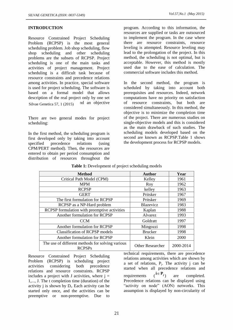
INTRODUCTION

Resource Constrained Project Scheduling

Problem (RCPSP) is the most general

scheduling problem. Job shop scheduling, flow

shop scheduling and other scheduling

problems are the subsets of RCPSP. Project

scheduling is one of the main tasks and

activities of project management. Project

scheduling is a difficult task because of

resource constraints and precedence relations

among activities. In practice, special software

is used for project scheduling. The software is

based on a formal model that allows

description of the real project only by one set

of scheduling constraints and an objective

function [1].

There are two general modes for project

scheduling:

In the first method, the scheduling program is

first developed only by taking into account

specified precedence relations (using

CPM/PERT method). Then, the resources are

entered to obtain per period consumption and

distribution of resources throughout the

program. According to this information, the

resources are supplied or tasks are outsourced

to implement the program. In the case where

there are resource constraints, resource

leveling is attempted. Resource leveling may

lead to the prolongation of the project. In this

method, the scheduling is not optimal, but is

acceptable. However, this method is mostly

used due to the ease of calculation. The

commercial software includes this method.

In the second method, the program is

scheduled by taking into account both

prerequisites and resources. Indeed, network

computations have no priority on satisfaction

of resource constraints, but both are

considered simultaneously. In this method, the

objective is to minimize the completion time

of the project. There are numerous studies on

single-objective models and this is considered

as the main drawback of such studies. The

scheduling models developed based on the

second are known as RCPSP.Table 1 shows

the development process for RCPSP models.

Table 1: Development of project scheduling models

Year Author Method

1961 Kelley Critical Path Model (CPM)

1962 Roy MPM

1963 kelley RCPSP

1967 Pritsker GERT

1969 Pritsker The first formulation for RCPSP

1983 Blazevicz RCPSP as a NP-Hard problem

1988 Kaplan RCPSP formulation with preemptive activities

1993 Alvarez Another formulation for RCPSP

1997 Goldratt CCM

1998 Mingozzi Another formulation for RCPSP

1998 Brucker Classification of RCPSP models

2000 Klein Another formulation for RCPSP

2000-2014 Other Researcher The use of different methods for solving various

RCPSPs

Resource Constrained Project Scheduling

Problem (RCPSP) is scheduling project

activities considering both precedence

relations and resource constraints. RCPSP

includes a project with J activities, where j =

1,..., J. The t completion time (duration) of the

activity j is shown by Di. Each activity can be

started only once, and the activities can be

preemptive or non-preemptive. Due to

technical requirements, there are precedence

relations among activities which are shown by

a set of relations, Pj. The activity j can be

started when all precedence relations and

requirements ( jPi) are completed.

Precedence relations can be displayed using

“activity on node” (AON) networks. This

assumption is displayed by non-circularity of

Silvae Genetica 57, 1 (2015)


22

the network. Each activity needs a specified

amount of resources to be performed [1].

According to Blazewicz et al [2], RCPSP is a

strong NP-Hard problem. The mathematical

model of RCPSP was developed by Pritsker et

al.[3] The standard RCPSP model is shown by

maxCprecps representing a project

scheduling problem with precedence relations

between activities aimed at minimizing the

project completion time. Although the RCPSP

model described above is a very capable

model, it cannot cover all real situations.

Accordingly, researchers have developed

many general models for project scheduling

problem. These models often use the standard

RCPSP model as a starting point.

RCPSP Types

Various RCPSP types have been studied in

different modes. RCPSPs can be classified as

follows:

1- Based on the nature of activities

2- Based on required resources

3- Based on precedence relations

4- Based on the type of objective function

5- Based on the number of objective functions

6- Based on the number of projects

The classification criteria and sub-criteria in

the following chart will be explained in detail.

Classification Criteria

The n

ature

of Ac

tivity

Reso

urce

Typ

e

Type

of P

rece

denc

e

Relat

ion

Type

of

Objec

tive F

uncti

on

Numb

er of

Objec

tive F

uncti

on

Natur

e of

Objec

tives

Numb

er of

proje

ct

Single Mode/ Multi Mode

Preemptive/Non-Preemptive

Probability/ Difinite /Fuzzy

Renewable

Non-Renewable

Dual

Partially Renewable

Dedicated Resource

Resource capacities

varying with time

Continous Resource

Partial

GPR

Regular

Unregular

Single objective

Bi-objective

Multi-objective

Time-based objective

Current-value base objective

Cost-based objective

Renewable Resource

based objective

Non-Renewable Resource

based objective

Consistency based objective

Single Project

Multi Project

Figure 1: Classification of RCPSPs


23

Multi-objective resource-constrained

project scheduling problem

Obviously, in an ideal situation it is better to

consider more than one objective to implement

the project scheduling. Considering only one

objective to solve such problems may cause

large losses in practice. Consequently, some

authors have used multiple objectives in

project scheduling.

Nadtasmbon and Randaha [4] proposed a

broad practical approach for considering

multiple objectives by creating a weighted

objective function of multiple objective

functions. The weighted function includes

several functions such as cost minimization,

minimizing weighted tardiness, resource

leveling and the usage of non-renewable

resources.

Witt and Vob [5] studied a multimode RCPSP

with three objectives including cost

minimization, minimizing weighted tardiness

and minimizing the preparation costs. The

activities can be categorized by taking into

account the preparation costs. This was in fact

a production planning problem in a steel

factory. Haouri and Al-Fawzan [6] integrated

two objectives including maximization of the

total free float and minimization of the

completion time of the project. The other

solution for multi-objective RCPSPs is to

develop an optimal Pareto scheduling. Davis et

al [7] investigated minimization of the project

completion time and overuse of renewable

resources. Viana and de Sousa [8] integrated

minimization of the overuse of nonrenewable

resources and the weighted tardiness. Hapke et

al [9] used a multi-objective approach

involving time-based, resource-based and

financial goals.Slowiniski et al [10] examined

a multimode RCPSP with a variety of

objectives including minimizing the project

duration and the delay weight of all delayed

activities, leveling the resource profile, the

weight of consumed resources and the present

value.Dorner et al [11] examined a time-cost

trade-off problem with three objectives. The

first objective was minimizing the project

completion time. The second and third

objectives were monetary and non-monetary

costs of the failure of activities.According to

Brooker Classification, the optimal Pareto

scheduling can be shown as a vector of all

objective functions.Weglarz and Nabrzynski

[12] used a well-known approach for the

multimode project scheduling problem and a

set of critical times and costs. They studied the

project completion time and resource leveling,

the delay weight of workflow (time), the

weight of total consumed resources and the

present value. Table 2 summarizes the theses

on RCPSP in Iran:

Table 2: Iranian Thesis on RCPSP

Thesis Title University Year

1 Analysis of DH branch and bound method for solving

multi resource-constrained project scheduling problem, a

data structure model and computer program

Isfahan

University of

Technology

2000

2 Scheduling the multi-mode resource-constrained project

activities considering the time value of money using the

refrigeration simulation and the Tabu search

Tehran

University 2005

3 Resource-constrained project scheduling by genetic

algorithm

Iran University

of Science and

Technology

2002

4 Multi-criteria resource-constrained fuzzy planning using

genetic algorithm

Tehran

University 2005

5 An efficient genetic algorithm for solving the resource-

constrained project scheduling problems

Tehran

University 2006

6 A heuristic algorithm for project scheduling using the

critical chain

Tehran

University 2002

7 The design of database-oriented decision support system

for scheduling RCSPS network

Amirkabir

University 2003

8 A heuristic method for RCSPS

Isfahan

University of 1986


24

Technology

9 A heuristic algorithm for project scheduling problem to

maximize the net present value

Isfahan

University of

Technology

2002

1

0 An algorithm to apply constraint theory in project

scheduling

Tarbiat

Modarres

University

1998

1

1 A method based on PSO algorithm for RCSPS Bu-Ali Sina

University 2009

1

2 The design of a combined genetic algorithm for solving

multimode RCSPS

Tarbiat

Modarres

University

2011

1

3 RCSPS: completion time, capabilities and NPV using the

MOPSO meta-heuristic method

Bu-Ali Sina

University 2011

The proposed model for the multi-objective

RCPSP

According to literature, the models used to

solve RCPSP suffer from some deficiencies.

Developing these models, a more

comprehensive and applicable model can be

obtained. The proposed model is defined to

cover the weaknesses of the previous models.

Due to the multi-objective nature of the

problem, a multi-objective model is proposed

considering the major objectives and goals of

executives in the industry.

The proposed model includes three objectives

of minimizing completion time, minimizing

the project costs and maximizing the quality of

the project activities. The first objective

(completion time minimization) is the most

famous objective in this kind of problems. By

minimizing the completion time of the last

activity in the project, this objective can be

achieved. Another objective in today's world

despite the enormous economic constraints is

minimizing the project costs. In this study, this

objective will be achieved through minimizing

the cost of each activity in the execution mode.

The last objective is to maximize the quality of

the project activities. This objective is highly

regarded by employers and project managers

in recent years. In this research, this objective

will be realized by maximizing the geometric

mean of the quality of each activity. To obtain

a more comprehensive and applicable model,

the general precedence relations between

activities are considered. Below, the decision

variables, presumptions and constraints are

described.

The presumptions of the proposed model are

as follows:

1- “This is multimode deterministic problem.”

The proposed model is intended to be

deterministic and thus the probable modes are

not considered. Therefore, it is recommended

to develop this model to consider uncertainty

or fuzzy modes in the proposed problem. In

addition, multimode project activities can be

included in the model. In practice, an activity

can be fulfilled in several ways. Therefore,

multimode activities are considered in the

proposed model.

2- “After the start of each activity, stoppage is

not permitted.”

In this research, preemptive mode is not

considered in the proposed problem and thus

activities can be done or failed at various

times. Therefore, after the start of an activity,

it must be continuously done until the end.

3- “The capacity of resources is specified and

limited.”

In the proposed model, the resources are

limited, renewable and non-renewable. The

capacity of resources is limited and specified

at the beginning of the project. Items such as

project budget are also considered as

renewable resources.

4- “No preparation time is required to perform

activities.”


25

According to literature, a time is considered

for preparation of resources to start and

perform an activity. In the proposed model, no

preparation time is needed for various project

activities.

Indices i, j: The number of project activities

mi: The executive mode of the activity i

ti: The time interval between the earliest and

latest start times of the activity i

k: The renewable or non-renewable resource

type

i : The nonrenewable resource k

di: Completion time of the activity

The decision variable

The decision variable is a binary variable

called Ximt. If the activity i is started at time t

in the executive mode m Ximt= 1, otherwise

Ximt=0. Ximt is defined as follows:

iiiimt lsestMmnix ,..,;,...,2,1;,...,2,1}1,0{

Since this is a multimode problem, three

indices are used for the decision variable. The

first index, i, represents the corresponding

activity, m denotes the executive mode of the

activity i and t shows the completion time of

the activity i and t is a time between the

earliest and latest start time of the activity i.

Model parameters

The parameters of the model are as follows:

i Activity i

Mi The executive modes of the activity i

A The set of activities

qim The quality of implementation of the

activity i in the executive mode m

Lsi The latest start time for the activity i

Esi The earliest start time for the activity i

Cim The implementation cost of the

activity i in the executive mode m

EFs The finish-start set of precedence

relations

FSij Minimal or maximal lag time between

the start and completion of the activity

i, j

dim The duration of the activity i in mode

m

rimk The per period usage of (total resource

consumption) of the activity j of

renewable resource k in the execution

mode m

The availability of the renewable

resource type k at each period

The per period usage of (total resource

consumption) of the activity j of

nonrenewable resource k in the

execution mode m

The availability of the nonrenewable

resource type k in the entire project

Mathematical model

The mathematical model of the problem is as

follows:

S.t.

s.t.

[1]

[2]

imt

Ai Mm

im

ls

est

XcfMini

i

i

3

k

imkr

ka

AM

m

imtim

ls

estAi

i i

i

XqfMax

1

1

1

n

n

ls

est

tnxtfMin 12 .

imt

Ai Mm

im

ls

est

XcfMini

i

i

3

1

1

iM

m

ils

iest

imtX

1 1

( ) ( , )j ji i

i i i

i j

M lsM ls

im ij im t jm t fs

m t es m t es

t d FS X tx i j E

k

n

i

M

m

lst

esdts

imsimk

i i

iim

xr

1 1

},1min{

},max{


26

[3] K=1,…,K , t=1,….,T

[4] K=1… K , t=1,…., T

[5]

I=1,,,, n

[6]

Presumptions

This is a deterministic problem with

multimode activities.

After the start of each activity,

stoppage is not permitted.

The time required to perform a certain

activity is deterministic.

No preparation time is required to

perform activities.

The capacity of resources is specified

and limited.

An activity is implementable when

the prerequisites are completely done.

The objective functions

The first objective is to maximize the quality

of the entire project. The geometric mean of

the quality of all activities is used to measure

the quality of the entire project. Basically, the

geometric mean is used for scattered quality of

activities.

The second objective is to minimize the

completion time of the last activity. As a

result, the project completion time is

minimized. The third objective is to minimize

the total cost of the project.

Constraints There are several constraints in the proposed

problem including:

- Start time

According to Constraint (1), each activity can

be implemented in a single mode. In fact, if an

activity has several execution modes and an

execution mode is selected based on

conditions, the activity will be executed in that

mode by the end of the activity. The execution

mode cannot be converted into other execution

modes.

- Precedence relations

As mentioned, partial precedence relations are

considered in the proposed model. Constraint

(2) is the most common constraint in all

RCPSPs with partial precedence relations.

This is a Finish-Start (FS) constraint. This

constraint is applied to those activities that can

be performed after an activity.

- Renewable resources

Like in the basic RCPSP, constraint (3)

concerns renewable resources. All resources

with the maximum applicable capacity in each

period are included. Renewable constraints

such as manpower and equipment are also

included in this constraint.

- Nonrenewable resources

Constraint (4) concerns non-renewable

resources. The total amount of nonrenewable

resources is specified at the beginning of the

project. The nonrenewable resources are

gradually reduced by consumption. Resources

such as project funding, supplies and

consumables are nonrenewable resources. The

implementation cost of activities is minimized

through the third objective function. In

addition, project funding also can be

considered as a renewable resource. Thus, to

avoid additional costs, a new constraint is not

defined and the project budget constraint is

included in the constraint (4).

k

n

i

M

m

ls

ess

imsimk

i i

i

xr 1 1

i

ls

est

imt

M

m

im

i

i

xq 1

1,0imtx


27

- Quality

Finally, the constraint (5) ensures that the

quality of each activity is not lower than a

predetermined level. The calculation rule is

explained in the following sections.

Constraint (6) shows the binary decision

variable, Ximt.

The standard PSPLIB problems are used as a

benchmark for the new model. Here,

multimode RCPSP are used. The number of

execution modes and the completion time for

each activity are available. The only change is

the amount of resources available. The amount

of resources in the new problem is 2 times the

amount of resources available in the basic

MRCPSP model. This is permitted due to the

complexity and multi-objective nature of the

problem.

Bees Algorithm

The Bees Algorithm is a population-based

search algorithm which was developed in

2005. It mimics the food foraging behavior of

honey bee colonies. In its basic version the

algorithm performs a kind of neighborhood

search combined with random search, and can

be used for both combinatorial optimization

(for simultaneous optimization of several

variables) and functional optimization. A

colony of honey bees can extend itself over

long distances and in multiple directions

simultaneously to harvest nectar or pollen

from multiple food sources (flower patches).

The flower patches with high nectar or pollen

that may be collected with less effort are

searched by a large fraction of the colony. The

flower patches with low nectar or pollen

attract a small fraction of the colony. The food

foraging is started by scout bees searching for

promising flower patches (with high hopes of

nectar or pollen).

The scout bees move randomly from a flower

patch to another. During the harvest season

(flowering), the colony keeps a number of

scout bees ready to continue food foraging.

When all flower patches were searched, the

scout bees perform a ritual known as waggle

dance on a highly profitable food source.

Through the waggle dance a scout bee

communicates the location of the flower patch,

the distance to the flower patch and its quality

to idle bees. Using this data, the follower bees

will go to the highly profitable flower patches

[13].

Figure 2: The Bees Algorithm flowchart for multi-objective problems [14]

http://en.wikipedia.org/wiki/Search_algorithm

http://en.wikipedia.org/wiki/Combinatorial_optimization

http://en.wikipedia.org/wiki/Continuous_optimization

http://en.wikipedia.org/wiki/Honey_bees


28

Most of follower bees go to more promising

flower patches with higher hopes of nectar and

pollen. When all bees go to the same area, they

will be scattered around the flower patch due a

limited dancing range. Accordingly, not a

flower patch, but the best flowers in the flower

patch are indentified. The Bees Algorithm

evaluates each point in the parametric space

(consisting of possible solutions) as a food

source. The scout bees are simulated as

random agents to simplify the solution space.

They report the quality of the searched sites by

a merit function. Simplified solutions are

ranked. Other "bees" are new forces to search

the surrounding area of the solution space to

find the elite sites called “flower patch”. The

algorithm selectively searches other flower

patches to find the maximum point of the

merit function [15]. Figure 2 shows the

flowchart of the Bees Algorithm for single-

objective and multi-objective problems. The

flowchart mimics the food foraging behavior

of bees to find the best food resources. The

next figure is the flowchart of the Bees

Algorithm for multi-objective problems.

Bees Algorithm parameters

The Bees Algorithm needs the following

parameters

n= number of scout bees

m= number of sites selected out of n

previously visited sites

e= number of sites selected out of the m

selected sites

nep= number of bees recruited for the best e

sites

nsp= number of bees recruited for other (m-e)

selected sites

ngh= the initial size of patches including the

site, its neighborhood and the stopping

criterion

The algorithm is started by n soldiers (scout

bees) placed randomly in the search space. The

suitability of the sites searched by scout bees

is assessed in the step 2.

Step 1: The initial population with random

solutions

Step 2: Evaluate fitness of population

Step 3: Forming new population

Step 4: Select sites for neighborhood search

Step 5: Recruit bees for the selected places and

evaluate fitness

Step 6: Select the fittest bee from each patch

Step 7: Assign remaining bees to search

randomly and evaluate their fitness

Step 8: The end

The proposed Bees Algorithm for multi-

objective RCPSP

The Bee Algorithm steps for solving multi-

objective RCPSP are as follows:

The parameters of the proposed algorithm

- Number of scout bees

- Number of archive solutions

- Number of selected sites

- Number of the best sites

- Number of bees assigned to search the

neighborhood of selected sites

- Number of bees assigned to search the

neighborhood of the best sites

The neighborhood is defined as in the single-

objective mode.

The steps of the proposed algorithm

Step 1: generate an initial solution

The scout bees are randomly placed in sites

containing the values of all three objectives.

Step 2: Ranking based on the Pareto

solutions


29

In this step, the generated solutions are ranked.

The Pareto solutions that are not dominated by

any solution rank 1. In contrast, the non-

dominated solutions relative to the first ranked

solutions which are dominated relative to other

solutions rank 2. Similarly, all solutions are

ranked.

The crowding distance (CD) is obtained for

each solution and then the solutions are sorted

based on the Pareto rank and crowding

distance. Then, all initial scout bees are

located in the archive list.

Step 3: the main loop of the algorithm

In this step, the following items are executed

for a predetermined number of iterations:

First, the scout bees in the archive list are

selected. Novice bees are determined based on

the following formula:

Number of novice bees= number of scout bees

× number of best sites

Waggle dance is performed for best sites and

the bees search the neighborhood of the best

sites. At the same time, the above operations

are performed for other selected sites which

are not best solutions. A random number

between 0 and 1 is generated for the excluded

site. If the random number is smaller than 0.5,

bees will randomly search for other sites

within the solution interval. Otherwise, they

will search for neighborhood in the previous

solution site.

Step 4: Archive Solutions

Solutions generated by new bees are added to

the archived solutions. Then, the archive is

sorted by the Pareto ranking and crowding

distance according to Step 2.

If the number of archived solutions is greater

than the number of predetermined archived

solutions (here equal to 50), the solutions at

the end of the list will be deleted such that the

remainder of the archive is equal to the

predetermined value.

Step 5 (final step): Return to Step 3

Comparison of the proposed Bees

Algorithm and NSGA-II

According to the literature [16], NSGA-II

outperforms strong algorithms such as PSA,

SPEA-II used for multi-objective RCPSP.

Therefore, this algorithm is compared with the

Bees Algorithm used in this study. To

compare the two algorithms, a standard

mathematical problem called FON function is

used. FON is defined as follows:

Figure 3: The Pareto solutions of the NSGA-

II

Figure 4: The Pareto solutions of the Bees

Algorithm

As can be seen(Fig 3,4), both algorithms give

reasonable results for this problem, but the

Bees Algorithm outperforms the NSGA-II in

terms of the regularity of Pareto solutions.

To evaluate these two algorithms in the

proposed model, “regularity”, “number”,

“relative and qualitative criteria”, “scattering”

and CPU time are used.

0 0.2 0.4 0.6 0.8 10

0.1

0.2

0.3

0.4

0.5

0.6

0.7

0.8

0.9

1

f1

f 2

Front 1

))3

1(exp(1)( 2

3

1

1 i

ixxf


30

Here, some small and large RCPSPs including

j102-2, j122-8, j141-8 and j301-1 are solved.

These problems are generated by MATLAB

according to the proposed RCPSP. The graphs

are compared with each other.

- Setting parameters for solving multi-

objective RCPSP

The following parameters are set to solve the

above multi-objective problems:

Number of scout bees: 20

Number of archived solutions: 50

Number of selected sites: 10

Number of best sites: 5

Number of bees assigned to search the

neighborhood of the selected sites: 10

Number of bees assigned to search the

neighborhood of the best sites: 30

To set the parameters, those influencing the

criteria were determined by solving various

problems. For this purpose, a variable

parameter was selected and other parameters

were fixed. The problems were solved several

times and the results were analyzed.

According to the results, the number of scout

bees and the number of bees assigned to the

selected sites and those assigned to the best

sites influence the performance of algorithm,

but other parameters have a very significant

impact on the results. Therefore, these three

parameters were adjusted.

To set the influencing parameters, an interval

was defined for each parameter according to

standard problems in the literature. Then, the

standard problems were solved using the

parameters with specified intervals. According

to the results, the value leading to the best

solution for multi-objective problems

including CPU time and the objective function

values was determined as the optimum value

of parameter.

The performance of two algorithms in

terms of “number”

The Bees Algorithm and NSGA-II were

compared according to the criteria defined in

the previous section. Table 2 summarizes the

results obtained for the criterion “number”

Table 3: Comparison of Bees Algorithm and NSGA-II in terms of “number”

NSGA-II Bees

Algorithm

Criterion Number

Problem

32 35 J102-2

30 35 J122-8

28 35 J141-8

31 33 J203-2

33 41 J301-1

As is clear from Table 2, the Bees Algorithm

outperforms the NSGA-II in terms of the

criterion “number” in all problems with

different sizes.

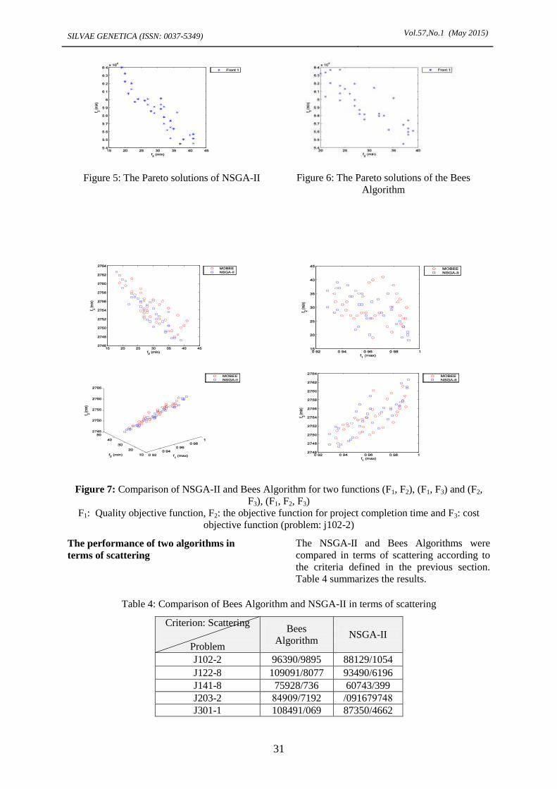
Figures 5 and 6 show the Pareto solutions of

j102-2 generated by NSGA-II and the Bees

Algorithm, respectively.


31

Figure 5: The Pareto solutions of NSGA-II


Algorithm

Figure 7: Comparison of NSGA-II and Bees Algorithm for two functions (F1, F2), (F1, F3) and (F2,

F3), (F1, F2, F3)

F1: Quality objective function, F2: the objective function for project completion time and F3: cost

objective function (problem: j102-2)


terms of scattering

The NSGA-II and Bees Algorithms were

compared in terms of scattering according to

the criteria defined in the previous section.

Table 4 summarizes the results.

Table 4: Comparison of Bees Algorithm and NSGA-II in terms of scattering

NSGA-II Bees

Algorithm

Criterion: Scattering

Problem

88129/1054 96390/9895 J102-2

93490/6196 109091/8077 J122-8

60743/399 75928/736 J141-8

/091674797 79444/7192 J203-2

87350/4662 108491/069 J301-1


32


the problem, j 122-8, generated by NSGA-II

and Bees Algorithm, respectively. As shown

in Table 4, the Bees Algorithm outperforms

the NSGA-II in all problems with various

tasks.



Algorithm

Figure 10: Comparison of NSGA-II and bees algorithm for two functions (F1, F2), (F1, F3) and (F2, F3),

(F1, F2, F3) F1: Quality objective function, F2: the objective function for project completion time and

F3: cost objective function (problem: j122-8)


terms of regularity

The NSGA-II and bees algorithms were

compared in terms of regularity according to

the criteria defined in the previous section.

Table 5 summarizes the results.

Table 5: Comparison of Bees Algorithm and

NSGA-II in terms of regularity

NSGA-

II

Bees

Algorithm

Criterion:

Regularity

Problem

0/4103 0/58989 J102-2

0/86105 0/83146 J122-8

0/87667 0/69209 J141-8

4/29746 4/71417 J203-2

0/66011 0/62211 J301-1


33


the problem, j 141-8, generated by NSGA-II

and Bees Algorithms, respectively. As shown

in Table 5, the Bees Algorithm outperforms

NSGA-II algorithms in most problems expect

for problems with 10 and 20 activities.


Figure 12: The Pareto solutions of bees algorithm

Figure 13: Comparison of NSGA-II and bees algorithm for two functions (F1, F2), (F1, F3) and (F2, F3),

(F1, F2,F3) F1: Quality objective function, F2: the objective function for project completion time and

F3: cost objective function (standard problem: j 203-2)


terms of relative and qualitative criteria

According to the criteria defined in the

previous section, the NSGA-II and bees

algorithms were compared in terms of relative

and qualitative criteria. Table 6 summarizes

the results.

Table 6: Comparison of Bees Algorithm and

NSGA-II in terms of relative and qualitative

criteria


34

NSGA-

II

Bees

Algorithm

Criterion: Relative

and qualitative

Problem

0/55357 0/54643 J102-2

0/63636 0/56364 J122-8

0/175 0/825 J141-8

4/725 4/675 J203-2

0/77083 0/72917 J301-1

In this case, NSGA-II outperforms the Bees

Algorithm. In contrast, the Bees algorithm

outperforms NSGA-II in J14 series problem. It

should be noted the difference between the

results is negligible as compared with other

criteria.


terms of CPU Time

Table 7: Comparison of the Bees Algorithm

and NSGA-II in terms of CPU time

NSGA-II Bees

Algorithm

Criterion:

CPU Time

(s)

Problem

74/1694 74/4429 J102-2

77/7491 79/6999 J122-8

44/6491 77/4192 J141-8

146/4614 47/4991 J203-2

164/4991 169/7169 J301-1

Of important criterion used to compare the

meta-heuristic algorithms is CPU time to

obtain a solution. Therefore, the NSGA-II and

Bees Algorithm were compared in terms of

CPU time. Obviously, with increasing the

number of activities, the time to achieve a

solution is increased. But in all cases, the Bees

Algorithm reaches the final result sooner with

the same number of iterations as compared

with NSGA-II. To implement both algorithms,

a computer with 2.1 GHz CPU and Windows

XP operating system was used. Since the

problem was solved in MATLAB software,

surely the time to solve these problems is

comparable to other algorithms used for

solving this problem. Almost all of them have

been programmed by C++ or Java and thus are

not comparable. Thus, only CPU times for j30

and j60 and j120 series are given and CPU

times are not compared with other algorithms.

Accordingly, it is recommended programming

the algorithm by C or Java to examine the

performance of the algorithm in terms of CPU

time.

Comprehensive analysis of the bees and the

NSGA-II algorithm

To evaluate the performance of the algorithm,

the performance of the proposed algorithm in

solving small and large problems was

investigated in detail. The results are given the

following tables and figures. The results show

the relative superiority of the Bees Algorithm.

For this purpose, 20 small problems (j10, j12,

j14, j 16 series) and 20 large problems (j18,

j20 and j30) were selected and solved by both

algorithms. The results are given in Table 8.

Table 8: The performance of NGSA-II and Bees Algorithm in solving small problems

Small

problems

Number Scattering Regularity

Relative and

qualitative

MOBEE

NSGA-

II MOBEE NSGA-II MOBEE

NSGA-

II MOBEE

NSGA-

II

1 j102-4 36 32 1839150.851 1612700.15 0.58352 0.61364 0.66038 0.33962

2 j104-2 32 35 1497739.15 1613744.11 0.89318 1.036 0.35849 0.64151

3 j106-3 36 35 2523933.408 2443121.95 0.62875 0.75111 0.39655 0.60345

4 j108-6 32 34 1661382.631 1763999.3 0.65665 0.89325 0.45455 0.54545

5 j1011-5 40 36 2177656.797 2032103.86 0.52433 0.75618 0.76923 0.23077

6 j1064-10 37 38 2082972.302 2138625.77 0.95624 0.62958 0.36207 0.63793

7 j1211-2 33 40 1957940.852 1979058.2 0.69657 0.80428 0.8722 1

8 j1211-10 36 36 2443121.949 1832490.31 0.63441 0.8996 0.39655 0.39655

9 j12-12-7 41 34 2751256.849 2240360.6 0.77645 0.83215 0.67857 0.32143


35

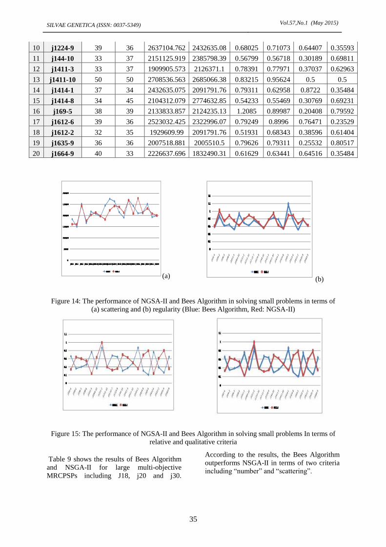
10 j1224-9 39 36 2637104.762 2432635.08 0.68025 0.71073 0.64407 0.35593

11 j144-10 33 37 2151125.919 2385798.39 0.56799 0.56718 0.30189 0.69811

12 j1411-3 33 37 1909905.573 2126371.1 0.78391 0.77971 0.37037 0.62963

13 j1411-10 50 50 2708536.563 2685066.38 0.83215 0.95624 0.5 0.5

14 j1414-1 37 34 2432635.075 2091791.76 0.79311 0.62958 0.8722 0.35484

15 j1414-8 34 45 2104312.079 2774632.85 0.54233 0.55469 0.30769 0.69231

16 j169-5 38 39 2133833.857 2124235.13 1.2085 0.89987 0.20408 0.79592

17 j1612-6 39 36 2523032.425 2322996.07 0.79249 0.8996 0.76471 0.23529

18 j1612-2 32 35 1929609.99 2091791.76 0.51931 0.68343 0.38596 0.61404

19 j1635-9 36 36 2007518.881 2005510.5 0.79626 0.79311 0.25532 0.80517

20 j1664-9 40 33 2226637.696 1832490.31 0.61629 0.63441 0.64516 0.35484

(b) (a)

Figure 14: The performance of NGSA-II and Bees Algorithm in solving small problems in terms of

(a) scattering and (b) regularity (Blue: Bees Algorithm, Red: NGSA-II)

Figure 15: The performance of NGSA-II and Bees Algorithm in solving small problems In terms of

relative and qualitative criteria

Table 9 shows the results of Bees Algorithm

and NSGA-II for large multi-objective

MRCPSPs including J18, j20 and j30.

According to the results, the Bees Algorithm

outperforms NSGA-II in terms of two criteria

including “number” and “scattering”.


36

Table 9: The performance of Bees Algorithm and NSGA-II in solving large problems

Large

problems

Number Scattering Regularity

Relative and

qualitative

MOBEE NSGA-

II MOBEE NSGA-II MOBEE

NSGA-

II MOBEE

NSGA-

II

1 j181-1 37 36 1085767.516 105681.7881 0.6926 0.68306 0.55556 0.44444

2 j1810-6 33 33 1097612.673 1081743.445 0.76626 0.76626 0.36872 0.46513

3 j1812-2 33 35 1675511.336 1631433.53 0.632 0.67321 0.75432 0.73144

4 j1812-9 38 38 1092453.633 1093534.524 0.78445 0.6723 0.8791 0.85632

5 j1821-1 40 41 2198343.342 2298843.111 0.6421 0.67622 0.5681 0.67132

6 j2011-8 36 33 1091636.622 1060042.94 0.70381 1.064 0.72 0.48

7 j2012-8 37 37 1894211.633 1954465.345 0.3463 0.5352 0.53 0.6722

8 j2030-1 39 40 1979058.203 1909915.573 0.89325 0.89987 0.67857 0.67857

9

j2030-

10 35 35 187531.131 186632.1313 0.5653 0.7632 0.61 0.57913

10 j2050-7 35 36 2637304.762 2432635.075 0.62103 0.71073 0.64417 0.75593

11 j2061-8 39 36 2637104.762 2432635.075 0.68025 0.71324 0.64407 0.45391

12 j2062-1 34 33 1408232.322 1058232.421 0.5211 0.6792 0.5613 0.6711

13

j2064-

10 36 36 1872431.231 1866131.001 0.4421 0.7619 0.8713 0.6721

14 j304-1 36 41 105655.7086 1260267.683 0.60549 0.72183 0.7069 0.52778

15 j304-3 40 38 147611.3211 1466671.313 0.8101 0.67813 0.6711 0.78131

16 j305-2 38 38 107903.4213 1086932.434 0.67432 0.64533 0.65242 0.59083

17 j304-10 37 35 1198776.322 1187763.434 0.7832 0.69024 0.6732 0.7133

18 j309-9 42 42 189123.131 183432.2412 0.7523 0.7632 0.67452 0.59032

19 j3050-6 39 40 2179058.203 2092915.573 0.89325 0.89987 0.67857 0.67857

20

j3064-

10 40 42 121740.7972 127806.096 0.64304 0.82878 0.50755 0.79245

For the ease of comparison, the results listed in Table 9 are depicted in Figures 16 and 17.


37

(a)

(b)

Figure 16: The performance of the Bees Algorithm and NSGA-II in solving large problems

in terms of number and scattering

(a)

(b)

Figure 17: The performance of the Bees Algorithm and NSGA-II algorithms in solving large

problems

in terms of (a) regularity and (b) the relative

and qualitative criteria

Conclusion The present paper proposed a multi-objective

mathematical model with the most important

objectives in the real world to solve the

multimode project scheduling problem. The

problem was then solved by the meta-heuristic

Bees Algorithm. According to the literature,

NGSA-II outperforms other algorithms in

solving multi-objective problems. Thus, the

results were compared with the results of

NSGA-II. The results demonstrated the good

performance of the meta-heuristic Bees

Algorithm. It is recommended to develop the

mathematical model proposed in this study to

replace the partial precedence relations with

general precedence relations (GPR). In

addition, the preparation time can be included

in the model to develop a more complex and

more practical problem.

References

1. Demeulemeester W S.,.Herrolen W S,2002,

Project Scheduling,Kluwer Academic

Publishers.

2. Blazewicz J., Lenstra J.K., Rinnooy Kan

A.H.G.,1983 , Scheduling subject to resource

constraints: Classification and complexity,

Discrete Applied Mathematics 5,11-24

3. Pritsker A.A.B., Watters L.J., Wolfe

P.M.,1969,, Multiproject scheduling with

limited resources: A zero-one programming

approach, Management Science6,93-107.


38

4. Sadeghi A.,Kalanaki A,Noktehdan A.,Safi

Samghabadi A. and Barzinpour F., 2011,Using

Bees Algorithm to Solve the Resource

Constrained. Project Scheduling Problem in

PSPLIB, Communications in Computer and

Information Science Volume 164, pp 486-494

5. Vos S., Witt A,2007, Hybrid flow shop

scheduling as a multi-mode multiproject

scheduling problem with batching

requirements: A real-world

application,International Journal of Production

Economics ,105,2,445-458.

6. Al-Fawzan M., Haouari M., ,2005, A bi-

objective model for robust resource

constrained project scheduling, International

Journal of Production Economics ,96,175-187.

7. Davis K.R., A. Stam, R.A. Grzybowski, 1992,

Resource constrained project scheduling with

multiple objectives: A decision support

approach, Computers and Operations Research

,19,7,657-669

8. Viana A., de Sousa J.P,2000, Using

metaheuristics in multi objective

resourceconstrained project scheduling,

European Journal of Operational Research,

120,359-374.

9. Ling Wang, Chen Fang, Ponnuthurai

Nagaratnam Suganthan, Min Liu , 2014,

Solving system-level synthesis problem by a

multi-objective estimation of distribution

algorithmOriginal Research Article, Expert

Systems with Applications, Volume 41, Issue

5, Pages 2496-2513,

10. SLowinski R. , B. Soniewicki, J. 1994,

We_glarz, DSS for multiobjective project

scheduling, European Journal of Operational

Research, 79, (2) , 220–229.

11. Dorner K.F., Gutjahr W.J., Hartl R.F., Strauss

C., Stummer C.,2008, Natureinspired

metaheuristics for multiobjective activity

crashing, Omega 3,6,1019-1037.

12. Blazewicz J., Ecker K., Pesch E., Schmidt G.,

Weglarz J.,2007, Handbook on Scheduling,

Springer, Berlin, Germany.

13. Pham D.T., Ghanbarzadeh A. ,2007, Multi-

Objective Optimisation using the Bees

Algorithm, Proceedings of IPROMS

Conference

14. Pham D. T. and Ghanbarzadeh A., 2007.

Multi-Objective Optimisation using the Bees

Algorithm,3rd International Virtual

Conference on Intelligent Production

Machines and Systems (IPROMS2007),

Whittles, Dunbeath, Scotland.

15. Amir Sadeghi; Abolfazl Kalanaki; Azadeh

Noktehdan; Azamdokht Safi Samghabadi;

Farnaz Barzinpour,2011,Using Bees Algorithm

to Solve the Resource Constrained Project

Scheduling Problem in PSPLIB,

Communications in Computer and Information

Science, 486-494.

16. Francisco Ballestín, Rosa Blanco , January

2011, Theoretical and practical fundamentals

for multi-objective optimisation in resource-

constrained project scheduling problems

Original Research Article , Computers &

Operations Research, Volume 38, Issue 1,

Pages 51-62.

http://link.springer.com/bookseries/7899

http://link.springer.com/bookseries/7899

the solution of multi-objective multimode resource ... · `silvae genetica (issn: 0037-5349)...

Documents