the solutions of nonlinear heat conduction equation via ...the solutions of nonlinear heat...
TRANSCRIPT
The Solutions of Nonlinear Heat Conduction Equation via Fibonacci&Lucas
Approximation Method
Zehra Pınara Turgut Öziş
b
aNamık Kemal University, Faculty of Science & Letters, Department of Mathematics, , 59030
Tekirdağ, Turkey
bEge University, Science Faculty, Department of Mathematics, 35100 Bornova-İzmir, Turkey
Abstract: To obtain new types of exact travelling wave solutions to nonlinear partial differential
equations, a number of approximate methods are known in the literature. In this study, we extend
the class of auxiliary equations of Fibonnacci&Lucas type equations. The proposed
Fibonnacci&Lucas approximation method produces many new solutions. Consequently, we
introduce new exact travelling wave solutions of some physical systems in terms of these new
solutions of the Fibonacci&Lucas type equation. In addition to using different ansatz, we use
determine different balancing principle to obtain optimal solutions.
Key Words: Nonlinear heat conduction equation, Fibonacci&Lucas equation, travelling wave
solutions, nonlinear partial differential equation, auxiliary equation
b Corresponding author: Zehra Pınar ([email protected] , +90282 2552706)

1. Introduction
The inspection of nonlinear wave phenomena physical systems is of great interest from both
mathematical and physical points of view. In most cases, the theoretical modeling based on
nonlinear partial differential equations (NLPDEs) can accurately describe the wave dynamics of
many physical systems. The critical importance is to find closed form solutions for NLPDEs of
physical significance. This could be a very complicated task and, in fact, is not always possible
since in various realistic problems in physical systems. So, searching for some exact physically
significant solutions is an important topic because of wide applications of NLPDEs in biology,
chemistry, physics, fluid dynamics and other areas of engineering[2,3].
Since many of the most useful techniques in analysis are formal or heuristic the trend in recent
years has also been to justify and provide the new procedures or methods rigorously[18]. Hence,
over the past decades, a number of approximate methods for finding travelling wave solutions to
nonlinear evolution equations have been proposed/or developed and furthermore modified [6-
20]. The solutions to various evolution equations have been found by one or other of these
methods. The technique of these methods consist of the solutions of the nonlinear evolution
equations such that the target solutions of the nonlinear evolution equations can be expressed as
a polynomial in an elementary function which satisfies a particular ordinary differential
equation. Recently, to determine the solutions of nonlinear evolution equations, many exact
solutions of various auxiliary equations have been utilized [22-27].
In this paper, we will examine the consequences of the choice of the Fibonacci&Lucas type
equation for determining the solutions of the nonlinear evolution equation in consideration and
more we search for additional forms of new exact solutions of nonlinear differential equations
which satisfying Fibonacci&Lucas type equation(s). To obtain wave solutions of nonlinear
partial differential equations via Fibonacci&Lucas transformation n optimal index value is
proposed.
2. Fibonacci & Lucas Polynomials
In this section, we determine Fibonacci&Lucas polynomials. Ordinary differential equations
satisfied by two families of Fibonacci and Lucas polynomials are derived using identities which
relate them to the generalized polynomials, and nonpolynomial solutions are deduced from
corresponding solutions of the partial differential equations.
The single variable polynomials (1, ) and (1, ), 0,n nF z L z n with the properties
( , ) (1, ),
( , ) (1, ),
n
n n
n
n n
F x y x F
L x y x L
where 2/y x , are referred to as the Fibonacci and Lucas polynomials, respectively, by Doman
and Williams [1]. Galvez and Devesa [4] have shown that they satisfy the ordinary differential
equations
Using the earlier results, it can be shown that a second linearly independent solution of the
Eq.(1) is (1, ) / 1 4nL , and a second linearly independent solution of the Eq.(2) is
1 4 (1, )nF .
The polynomials ( ,1) and ( ,1),n nF L also referred to as Fibonacci and Lucas polynomials by
Hoggatt and Bicknell [5], are related to the generalized polynomials by
( 1) / 2 / 2( , ) ( ,1), ( , ) ( ,1),n n
n n n nF x y y F L x y y L
where /x y , that they satisfy the ordinary differential equations
2
2 2
2
22 2
2
(4 ) 3 ( 1) 0, (3)
(4 ) 0,
n nn
n nn
d F dFn F
d d
d L dLn L
d d
(4)
which also have solutions 2 2( ,1) / 4 and 4 ( ,1)n nL F , respectively.
As seen above, Eqs(1)-(4) are depends on n index value, so the solutions of Eqs(1)-(4) are different
solutions for each n index values. But, one of the important questions is ‘Which n index value produce
an available basis for the given problem?’ and the answer is given in the following section.
3. Methodology
2
2
2
2
(1 4 ) [( 1) 2(2 5) ] ( 1)( 2) 0, (1)
(1 4 ) [( 1) 2(2 3) ] ( 1) 0.
n nn
n nn
d F dFn n n n F
d d
d L dLn n n n L
d d
(2)

The fundamental nature of the auxiliary equation technique is given by many authors in the
literature [6-15] and it is applied to this new approximation . Let us have a nonlinear partial
differential equation
( ) (5)
and let by means of an appropriate transformation which is depended on Fibonacci&Lucas type
equation(s), this equation is reduced to nonlinear ordinary differential equation
( ) . (6)
For large class of the equations of the type (6) have exact solutions which can be constructed via
finite series
( ) ∑ ( )
(7)
Here, ( ) are parameters to be further determined, is an integer fixed by a
balancing principle and elementary function ( ) is the solution of some ordinary differential
equation referred to as the auxiliary equation[15,16,17,19, 21].
It is worth to point out that we happen to know the general solution(s), ( ), of the auxiliary
equation beforehand or we know at least exact analytical particular solutions of the auxiliary
equation.
The outline of the method:
A) Define the solution of Eq.(6) by the ansatz in form of finite series in Eq.(7) where (
) are parameters to be further determined, is an integer fixed by a balancing
principle and elementary function ( ) is the solutions of Eqs(1-4) be considered which are
depended on n index values which helps us to obtain wave solution for the given problem. But,
for each n index values, we obtain different solutions of auxiliary equations(1)-(4), so we need to
determine n index values to control the availability of the given problem. To determine n
index values of Fibonacci&Lucas function from the balancing principle we proposed a novel
balancing given below
is highest degree
1,0,1 mod( )
m
m
u
n m
(8)
B) Substitute Eq.(7) into ordinary differential equation Eq.(6) to determine the parameters
( ) with the aid of symbolic computation.

C) Insert predetermined parameters and elementary function ( ) of the auxiliary equation
into Eq.(7) to obtain travelling wave solutions of the nonlinear evolution equation in
consideration.
It is very apparent that determining the elementary function ( ) via auxiliary equation is
crucial and plays very important role finding new travelling wave solutions of nonlinear
evolution equations. This fact, indeed, compel researchers to search for a novel auxiliary
equations with exact solutions.
In this study, we use Fibonacci& Lucas differential equations are given above.
4. Travelling Wave Solutions of Nonlinear Heat Conduction Equation In Terms of
Fibonacci&Lucas Equation Regarding As An Ansatz.
In this section, we consider the following nonlinear heat conduction equation
2 2 0 (9)t xxu u pu qu
where ,p q are real constants. To use Fibonacci&Lucas approximation method, we consider the
determined variables , instead of the wave variable. Although the wave transformation is not used to
obtain the wave solution, it is obtained by Fibonacci&Lucas transformations which are determined by
, . The , variables carries Eq. ( ) into the ordinary differential equation.
From the balancing principle, is obtained. Therefore, the ansatz yields
0 1( ) ( ) (10)U g g z
where ( )z may be determined by the solution of Eqs.(1)-(4).
Case 1: We consider 2/y x transformation and Eq(1) is considered as an auxiliary equation,
The variables carries Eq. ( ) into the ordinary differential equation
2
2 2 3
2 6 6 4
( ) ( ) ( ) ( )8 8 ( ) 12 ( ) ( ) ( ) 0 (11)
U U U Ut U t U t pU qU
x x x x
and here the ansatz is assumed as following
Hence, substituting Eqs.(1) and(12) into Eq.(11) and letting each coefficient of ( )nF to be zero,
we obtain algebraic equation system and solving the system by the aid of Maple 16, we can
determine the coefficients:
0 1( ) ( ) (12)nU g g F

2
1 1 2 2 0 2
2 3 3 3 2 3 3 2 2 2 2 2 3 2 4 3 2 2 2 2
1 2
8 (2 3 )) , ,
3 (1 )
64 2144 256 1312 1088 3 6 21 48 24 64 160 32
12 (1 ) (1 17 2 8 )
n ni C C C C g
qx
n n n qx qx qx qx qx n n ng
qx n n
2 7
1 1 2 2 2 3
1 1
2
0 2
(1 )) ,
5( 1 12 36 8 8 )
8 (2 3 )
3 (1 )
pxii C C C
g g
n ng
qx
Substituting the above coefficients into ansatz (12) with the solution of Lucas type equation, we
obtain one of new solution of nonlinear heat conduction equation.
2 2 3 3 3 2 3 3 2 2 2 2 2 3 2 4 3 2 2 2 2
2 2
1
8 (2 3 ) 64 2144 256 1312 1088 3 6 21 48 24 64 160 32( , )
3 (1 ) 12 (1 ) (1 17 2 8 )
n n n n n qx qx qx qx qx n n nu x t
qx qx n n
C hyperge
2 2
2
( 8 3 ) 2 2
2 2 2
9 73 60 12 9 73 60 122 , 2 ,[ 3 9],1
2 2 2 2
7 73 60 12 7 73 60 121 , ,[ 7 3 ],1
2 2 2 2
n
n n n n tom n n n
x
t n n n n tC hypergeom n n n
x x
2 2
1 22
12( 8 3 )2 7 2
2 2 3 2
1 1
9 73 60 12 9 73 60 122 , 2 ,[ 3 9],1
2 2 2 28 (2 3 )
( , )3 (1 )
(1 ) 7 73 60 12 7 71 ,
5( 1 12 36 8 8 ) 2 2 2
n
n n n n tC hypergeom n n n
xn n
u x t gqx
px t n nhypergeom n n
g g x
2
2
3 60 12,[ 7 3 ],1
2
n n tn
x
To obtain suitable solution, 1n is obtained from Eq(8).For the special values of parameters,
the solutions are shown in Figure 1.

(a) (b)
Figure 1. (a) is for the first solution for 2 12, 1, 0.5, 1C q C n , (b) is for the second
sloution where 1 11, 1, 1, 1p C g n ,
If n index values are chosen arbitrary, not using balancing formula Eq(8), the solutions of
Eqs(1)-(4) don’t construct a basis for the given equation. In that case, the behavior of solutions
changes respect to n index values. Therefore, to obtain travelling wave solutions for the given
equation, we need to use the balancing formula Eq(8). For this example, if n index values are
taken as 2,3,4,...n , which are not satisfy the Eq(8), then for these index values we don’t
obtain solutions or these index values distort wave behavior of the obtained solutions. It is seen
in the Figure 2.
(a) (b)

Figure 2. (a) is for the 2n index value, (b) is for the 4n index value
Case 2: We consider /x y transformation and Eq(4) is considered as an auxiliary
equation. The variables carries Eq. ( ) into the ordinary differential equation
2
3
3/ 2
( ) ( ) ( )2 2 ( ) ( ) ( ) 0 (13)
2
U x U UU pU qU
t t t
and here the ansatz is assumed as following from the balancing principle
Hence, substituting Eqs.(4) and(14) into Eq.(13) and letting each coefficient of ( )nL to be zero,
we obtain algebraic equation system and solving the system by the aid of Maple 16, we can
determine the coefficients:
1 1 2 2 0 1 1, , , , 0,C C C C n n p p g g g
and
2
2
1 1 2
1
22
2 2
2
0 1 122
2
2
4 arctan4
, , ,2
4arctan
4, 0,
4arctan (4 )
4
C C C n ng
p g g g
t
Substituting the above coefficients into ansatz (14) with the solution of Lucas type equation, we
obtain new solutions of nonlinear heat conduction equation.
2 22 2
1 1 22 2
1 1( , ) sin 8 2 arctan cos 8 2 arctan
2 24 4
n x x x xU x t x g C pt px C pt px
t tt x t x
2
2 2
1 12
1
4 arctan cos arctan4 4
( , ) sin arctan4
n
x x xx n
tx t x t xU x t x g C n
g tt x
To obtain optimal solution, 1n is obtained from Eq(8).For the special values of parameters,
the solutions are shown in Figure 3.
0 1( ) ( ) (14)nU g g L
(a) (b)
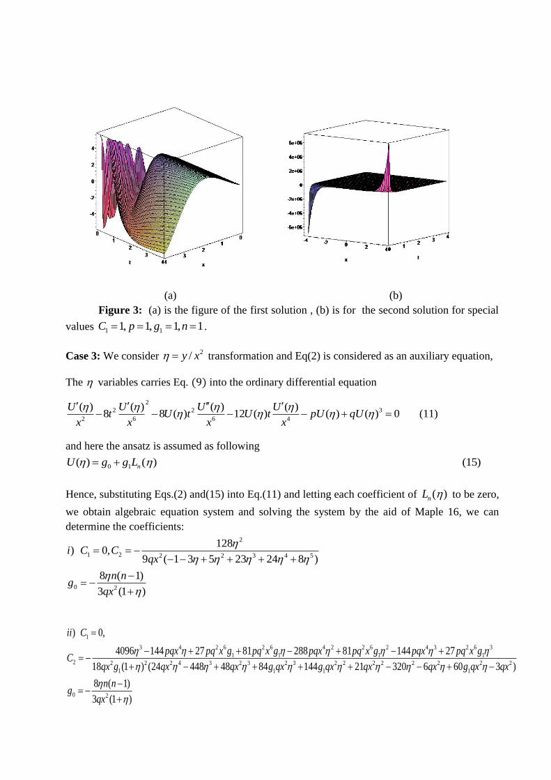
Figure 3: (a) is the figure of the first solution , (b) is for the second solution for special
values 1 11, 1, 1, 1C p g n .
Case 3: We consider 2/y x transformation and Eq(2) is considered as an auxiliary equation,
The variables carries Eq. ( ) into the ordinary differential equation
2
2 2 3
2 6 6 4
( ) ( ) ( ) ( )8 8 ( ) 12 ( ) ( ) ( ) 0 (11)
U U U Ut U t U t pU qU
x x x x
and here the ansatz is assumed as following
Hence, substituting Eqs.(2) and(15) into Eq.(11) and letting each coefficient of ( )nL to be zero,
we obtain algebraic equation system and solving the system by the aid of Maple 16, we can
determine the coefficients: 2
1 2 2 2 3 4 5
0 2
128) 0,
9 ( 1 3 5 23 24 8 )
8 ( 1)
3 (1 )
i C Cqx
n ng
qx
1
3 4 2 6 2 6 4 2 2 6 2 4 3 2 6 3
1 1 1 12 2 2 2 4 3 2 3 2 3 2 2 2 2 2 2 2 2
1 1 1 1
0
) 0,
4096 144 27 81 288 81 144 27
18 (1 ) (24 448 48 84 144 21 320 6 60 3 )
8 ( 1)
3
ii C
pqx pq x g pq x g pqx pq x g pqx pq x gC
qx g qx qx g qx g qx qx qx g qx qx
n ng
qx
2 (1 )
0 1( ) ( ) (15)nU g g L

4 3 4 3 3 4 2 2
2 6 4 2
3 3 2 2 3 2 3 3 2 2 2 2 2 3 2 4
1 2
0 2
2048 (2 5 1 35 33 8 3 51 9 ))
18 (1 ) ( 1 8 )
256 3 6 288 544 64 32 21 48 24
12 (1 )(2 8 1 9 )
8 ( 1)
3 (1 )
n n n n n n n n niii p
q x
n qx qx n n n n qx qx qxg
qx n n
n ng
qx
Substituting the above coefficients into ansatz (15) with the solution of Lucas type equation, we
obtain one of new solution of nonlinear heat conduction equation.
2 2
2( 4 3 )
2
12 2 2 2 3 4 5
3 25 36 12 3 25 36 12, ,[ 3 3 ],1
2 2 2 28 ( 1) 128( , ) 1
3 (1 ) 9 ( 1 3 5 23 24 8 )
n
n n n n thypergeom n n n
xn n tu x t g
qx x qx
3 4 2 6 2 6 4 2 2 6 2 4 3 2 6 3
1 1 1 1
2 2 2 4 3 2 3 2 3 2 2 2 2 2 2 24 1 1 1 1
2
4096 144 27 81 288 81 144 278 ( 1)( , )
18 (1 ) (24 448 48 84 144 21 320 6 60 33 1
pqx pq x g pq x g pqx pq x g pqx pq x gtn nu x t
t qx g qx qx g qx g qx qx qx g qx qqx
x
( 4 3 )
2 2
2 2
2
1)
3 25 36 12 3 25 36 12 , ,[ 3 3 ],1
2 2 2 2
nt
x x
n n n n thypergeom n n n
x
3 3 2 2 3 2 3 3 2 2 2 2 2 3 2 4
24
2
2
1
8 ( 1) 256 3 6 288 544 64 32 21 48 24( , )
12 (1 )(2 8 1 9 )3 1
5 25 36 122
2 2
tn n n qx qx n n n n qx qx qxu x t
t qx n nqx
x
n nC hypergeom n
2
2
( 4 3 ) 2 2
2 2 2
5 25 36 12, 2 ,[5 3 ],12 2
3 25 36 12 3 25 36 121 , ,[ 3 3 ],1
2 2 2 2
n
n n tn n
x
t n n n n tC hypergeom n n n
x x
To obtain optimal solution, 1n is obtained from Eq(8).For the special values of parameters,
the solutions are shown in Figure 4.
(a) (b)
(c)
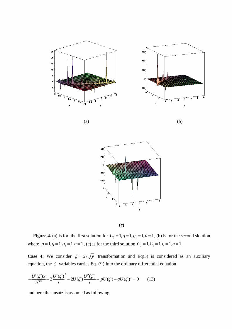
Figure 4. (a) is for the first solution for 2 11, 1, 1, 1C q g n , (b) is for the second sloution
where 11, 1, 1, 1p q g n , (c) is for the third solution 2 11, 1, 1, 1C C q n
Case 4: We consider /x y transformation and Eq(3) is considered as an auxiliary
equation, the variables carries Eq. ( ) into the ordinary differential equation
2
3
3/ 2
( ) ( ) ( )2 2 ( ) ( ) ( ) 0 (13)
2
U x U UU pU qU
t t t
and here the ansatz is assumed as following
Hence, substituting Eqs.(3) and(16) into Eq.(13) and letting each coefficient of ( )nF to be zero,
we obtain algebraic equation system and solving the system by the aid of Maple 16, we can
determine the coefficients:
2 2 4 3 2 2 2 6 5 2 4 3 2 8 7 2
1 2 1 2 1 2 1 2 1 21
2 2 4 3 2
1
32 8 4 32 18 4 64 32 4 10 8 4 16 16 4 4 32
4 4 2 4 4 4 2
g C g C g C g C g CC
g
Substituting the above coefficients into ansatz (16) with the solution of Lucas type equation, we
obtain one of new solution of nonlinear heat conduction equation.
2 2 2 4 3 2 2 2 6 5 2 4 3 2 8 7 2
1 2 1 2 1 2 1 2 1 2
1
2 2 4 3 2 2
12 2
4 32 8 4 32 18 4 64 32 4 10 8 4 16 16 4 4 32( , )
4 4 2 4 4 4 24 4
g C g C g C g C g Cu x t g
Cg
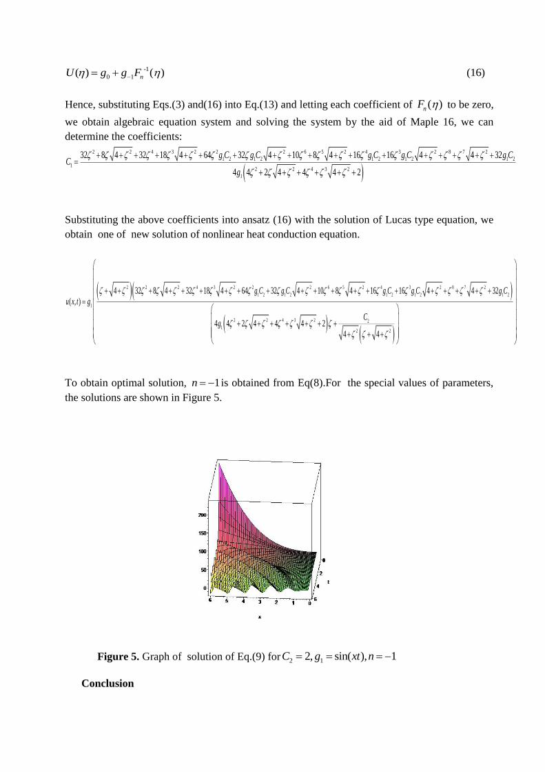
To obtain optimal solution, 1n is obtained from Eq(8).For the special values of parameters,
the solutions are shown in Figure 5.
Figure 5. Graph of solution of Eq.(9) for 2 12, sin( ), 1C g xt n
Conclusion
-1
0 1( ) ( ) (16)nU g g F
As it is seen, the key idea of obtaining new travelling wave solutions for the nonlinear equations
is using the exact solutions of different types equations as an ansatz. By means of
Fibonacci&Lucas type equation, the wave transformation is not used to obtain the wave
solutions, the Fibonacci&Lucas transformation is used to obtain the wave solutions. But, the
wave solutions are not obtained by the standard Fibonacci&Lucas transformations. For this
reason, the n optimal index value is proposed in Eq(8). Using the solutions of Fibonacci&Lucas
type equation, we have successfully obtained a number of new exact periodic solutions of the
nonlinear heat conduction equation by employing the solutions of the Fibonacci&Lucas type
equation regarding as an auxiliary equation in proposed method.
In this letter, we have obtained new solutions of the nonlinear equation in hand using the
Fibonacci&Lucas type equation (Eqs.(1-4)) for distinct cases. However, it is well known that the
n optimal index value produces new travelling wave solutions for many nonlinear problems.
The presented method could lead to finding new exact travelling wave solutions for other
nonlinear problems.
5. References
[1] B. G. S. Doman & J. K. Williams. "Fibonacci and Lucas Polynomials.'1 Math. Proc.
Cambridge Philos. Soc. 9.0 (1981):385-87.
[2] L.Debnath, Nonlinear partial differential equations for scientists and Engineers (2nd
ed.)
Birkhauser, Boston (2005)
[3] G.B.Whitham, A general approach to linear and nonlinear waves using a Lagrangian, J.
Fluid Mech.,22(1965) 273-283
[4] F. J. Galvez & J. S. Dehasa. "Novel Properties of Fibonacci and Lucas Polynomials."
MathProc. Cambridge Philos. Soc. 91 (1985): 159-6
[5] V. E. Hoggatt, Jr., & M. Bicknell "Roots of Fibonacci Polynomials." The Fibonacci
Quarterly 11.3 (1973):271-74
[6] C. Yong, L. Biao, Z. Hong-Quing, Generalized Riccati equation expansion method and
its application to Bogoyaylenskii’s generalized breaking soliton equation, Chinese Physics. 12
(2003) 940–946.2004.
[7] G. Cai, Q. Wang, J. Huang, A modified F-expansion method for solving breaking soliton
equation, International Journal of Nonlinear science 2(2006) 122-128
[8] X. Zeng, X. Yong, A new mapping method and its applications to nonlinear partial
differential equations, Phy. Lett. A. 372 (2008) 6602–6607.
[9] X. Yong, X. Zeng, Z. Zhang, Y. Chen, Symbolic computation of Jacobi elliptic function
solutions to nonlinear differential-difference equations, Comput.Math. Appl.
doi:10.1016/j.camwa2009.01.008.
[10] W. X. Ma, T. Huang, Y. Zhang, A multiple Exp-function method for nonlinear
differential equations and its applications, Phys. Scr. 82(2010) 065003(8pp)
[11] T. Ozis, I. Aslan, Symbolic computation and construction of New exact traveling wawe
solutions to Fitzhugh-Nagumo and Klein Gordon equation, Z. Naturforsch. 64a(2009) 15-20
[12] T. Ozis, I. Aslan, Symbolic computations and exact and explicit solutions of some
nonlinear evolution equations in mathematical physics, Commun. Theor. Phys., 51(2009) 577-
580
[13] Sirendaoreji, Auxiliary equation method and new solutions of Klein–Gordon equations,
Chaos, Solitons and Fractals 31 (2007) 943–950
[14] B. Jang, New exact travelling wave solutions of nonlinear Klein–Gordon equations,
Chaos, Solitons and Fractals 41 (2009) 646–654
[15] X. Lv, S. Lai, Y.H. Wu, An auxiliary equation technique and exact solutions for a
nonlinear Klein–Gordon equation, Chaos, Solitons and Fractals 41 (2009) 82–90
[16] E. Yomba, A generalized auxiliary equation method and its application to nonlinear
Klein–Gordon and generalized nonlinear Camassa–Holm equations, Physics Letters A 372
(2008) 1048–1060
[17] J. Nickel, Elliptic solutions to a generalized BBM equation, Physics Letters A 364
(2007) 221–226
[18] E.T. Whittaker, G.N. Watson, A Course of Modern Analysis, Cambridge Univ. Press,
Cambridge, 1927.
[19] E. Yomba, The extended Fan’s sub-equation method and its application to KdV-MKdV,
BKK and variant Boussinesq equations, Phys. Lett. A, 336(2005) 463-476
[20] Z. Y. Yan, An improved algebra method and its applications in nonlinear wave
equations,Chaos Solitons & Fractals 21(2004)1013-1021
[21] M.A. Abdou, A generalized auxiliary equation method and its applications, Nonlinear
Dyn 52 (2008) 95–102
[22] Z. Pinar, T. Ozis, An Observation on the Periodic Solutions to Nonlinear
Physical models by means of the auxiliary equation with a sixth-degree
nonlinear term, Commun Nonlinear Sci Numer Simulat, 18(2013)2177-2187
[23] N.K. Vitanov, Z. I. Dimitrova, K. N. Vitanov, On the class of nonlinear PDEs that can be
treated by the modified method of simplest equation. Application to generalized Degasperis–
Processi equation and b-equation, Commun Nonlinear Sci Numer Simulat 16 (2011) 3033–3044
[24] RI. Ivanov, Water waves and integrability, Phil Trans R Soc A, 365(2007) 2267–80
[25] L. Debnath, Nonlinear water waves, New York, Academic Press; 1994
[26] RS. Johnson, The classical problem of water waves: a reservoir of integrable and nearly-
integrable equations, J Nonlin Math Phys 10 (2003) 72–92
[27] N. K. Vitanov, Modified method of simplest equation: Powerful tool for obtaining exact
and approximate traveling-wave solutions of nonlinear PDEs, Commun Nonlinear Sci Numer
Simulat 16 (2011) 1176–1185

List of Figures
Figure 1. (a) is for the first solution for 2 12, 1, 0.5, 1C q C n , (b) is for the second
sloution where 1 11, 1, 1, 1p C g n ,
Figure 2. (a) is for the 2n index value, (b) is for the 4n index value
Figure 3: (a) is the figure of the first solution , (b) is for the second solution for special values
1 11, 1, 1, 1C p g n .
Figure 4. (a) is for the first solution for 2 11, 1, 1, 1C q g n , (b) is for the second sloution
where 11, 1, 1, 1p q g n , (c) is for the third solution 2 11, 1, 1, 1C C q n
Figure 5. Graph of solution of Eq.(9) for 2 12, sin( ), 1C g xt n