J. Math. Anal. Appl. 369 (2010) 712–718

Contents lists available at ScienceDirect

Journal of Mathematical Analysis andApplications

www.elsevier.com/locate/jmaa

The solvability and explicit solutions of two integral equations viageneralized convolutions

Nguyen Minh Tuan a,∗, Nguyen Thi Thu Huyen b

a Dept. of Math. Analysis, University of Hanoi, 334 Nguyen Trai Str., Hanoi, Viet Namb Dept. of Math., University of Phuong Dong, 201B Trung Kinh Str., Hanoi, Viet Nam

a r t i c l e i n f o a b s t r a c t

Article history:Received 9 November 2009Available online 10 April 2010Submitted by Goong Chen

Keywords:Generalized convolutionHermite functionIntegral equation of convolution typeNormed ring

This paper presents the necessary and sufficient conditions for the solvability of twointegral equations of convolution type; the first equation generalizes from integralequations with the Gaussian kernel, and the second one contains the Toeplitz plus Hankelkernels. Furthermore, the paper shows that the normed rings on L1(Rd) are constructed byusing the obtained convolutions, and an arbitrary Hermite function and appropriate linearcombination of those functions are the weight-function of four generalized convolutionsassociating F and F̌ . The open question about Hermitian weight-function of generalizedconvolution is posed at the end of the paper.

© 2010 Elsevier Inc. All rights reserved.

1. Introduction and statements of main results

The main aim of this paper is to solve the Fredholm integral equation

λϕ(x) + 1

(2π)d2

∫Rd

K (x, y)ϕ(y)dy = g(x) (1.1)

in the separate cases of kernel: K is of the form

K (x, y) = 1

(2π)d2

∫Rd

[k1(u)Φα(x − u − y) + k2(u)Φα(x + u − y)

+ k3(u)Φα(x − u + y) + k4(u)Φα(x + u + y)]

du, (1.2)

where Φα is the Hermite function or the appropriate linear combination of those functions, and K is sum of the Toeplitzand Hankel kernels, i.e.

K (x, y) = k1(x − y − h1) + k2(x − y + h2) + k3(x + y − h3) + k4(x + y + h4), (1.3)

where h1,h2,h3,h4 ∈ Rd (called shifts or delays) are given.

The integral equation (1.1) with the kernels (1.2), (1.3) attract attention of many authors as that with (1.2) generalizesfrom the equations with Gaussian kernel which has applications in radiative wave transmission and in many problemsof Medicine and Biology, and that with the kernel (1.3) has many useful applications in such diverse fields as scattering

* Corresponding author.E-mail address: tuannm@hus.edu.vn (N.M. Tuan).

0022-247X/$ – see front matter © 2010 Elsevier Inc. All rights reserved.doi:10.1016/j.jmaa.2010.04.019

N.M. Tuan, N.T.T. Huyen / J. Math. Anal. Appl. 369 (2010) 712–718 713

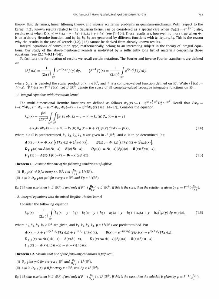
theory, fluid dynamics, linear filtering theory, and inverse scattering problems in quantum-mechanics. With respect to the

kernel (1.2), known results related to the Gaussian kernel can be considered as a special case when Φ0(x) = e− 12 |x|2 ; also,

results exist when K (x, y) = k1(x − y − h1)+k4(x + y + h2) (see [1–10]). Those results are, however, no more true when Φα

is an arbitrary Hermite function, and k1,k2,k3,k4 are generated by different functions with h1,h2,h3,h4. This is the reasonwhy the results in the case of kernels (1.2), (1.3) cannot be derived from already known results.

Integral equations of convolution type, mathematically, belong to an interesting subject in the theory of integral equa-tions. Our study of the above-mentioned kernels is motivated by a sufficiently long list of materials concerning thoseequations (see [2,5,7–9,11–14]).

To facilitate the formulation of results we recall certain notations. The Fourier and inverse Fourier transforms are definedas:

(F f )(x) = 1

(2π)d2

∫Rd

e−i〈x,y〉 f (y)dy,(

F −1 f)(x) = 1

(2π)d2

∫Rd

ei〈x,y〉 f (y)dy,

where 〈x, y〉 is denoted the scalar product of x, y ∈ Rd , and f is a complex-valued function defined on R

d . Write ( f̌ )(x) :=f (−x), ( F̌ f )(x) := (F −1 f )(x). Let L1(Rd) denote the space of all complex-valued Lebesgue integrable functions on R

d .

1.1. Integral equations with Hermitian kernel

The multi-dimensional Hermite functions are defined as follows Φα(x) := (−1)|α|e 12 |x|2 Dα

x e−|x|2 . Recall that FΦα =(−i)|α|Φα , F −1Φα = (i)|α|Φα , Φα(−x) = (−1)|α|Φα(x) (see [14–17]). Consider the equation

λϕ(x) + i|α|

(2π)d

∫Rd

∫Rd

[k1(u)Φα(x − u − v) + k2(u)Φα(x + u − v)

+ k3(u)Φα(x − u + v) + k4(u)Φα(x + u + v)]ϕ(v)du dv = p(x), (1.4)

where λ ∈ C is predetermined, k1,k2,k3,k4, p are given in L1(Rd), and ϕ is to be determined. Put

A(x) := λ + Φα(x)[(Fk1)(x) + ( F̌ k2)(x)

], B(x) := Φα(x)

[(Fk3)(x) + ( F̌ k4)(x)

],

D F , F̌ (x) := A(x)A(−x) − B(x)B(−x), D F (x) := A(−x)(Fp)(x) − B(x)(Fp)(−x),

D F̌ (x) := A(x)(Fp)(−x) − B(−x)(Fp)(x). (1.5)

Theorem 1.1. Assume that one of the following conditions is fulfilled:

(i) D F , F̌ (x) �= 0 for every x ∈ Rd, and D F

D F , F̌∈ L1(Rd).

(ii) λ �= 0, D F , F̌ (x) �= 0 for every x ∈ Rd, and Fp ∈ L1(Rd).

Eq. (1.4) has a solution in L1(Rd) if and only if F −1( D FD F , F̌

) ∈ L1(Rd). If this is the case, then the solution is given by ϕ = F −1( D FD F , F̌

).

1.2. Integral equations with the mixed Toeplitz–Hankel kernel

Consider the following equation

λϕ(x) + 1

(2π)d2

∫Rd

[k1(x − y − h1) + k2(x − y + h2) + k3(x + y − h3) + k4(x + y + h4)

]ϕ(y)dy = p(x), (1.6)

where h1,h2,h3,h4 ∈ Rd are given, and k1,k2,k3,k4, p ∈ L1(Rd) are predetermined. Put

A(x) := λ + e−i〈x,h1〉(Fk1)(x) + ei〈x,h2〉(Fk2)(x), B(x) := e−i〈x,h3〉(Fk3)(x) + ei〈x,h4〉(Fk4)(x),

D F , F̌ (x) := A(x)A(−x) − B(x)B(−x), D F (x) := A(−x)(Fp)(x) − B(x)(Fp)(−x),

D F̌ (x) := A(x)(Fp)(−x) − B(−x)(Fp)(x).

Theorem 1.2. Assume that one of the following conditions is fulfilled:

(i) D F , F̌ (x) �= 0 for every x ∈ Rd, and D F

D F , F̌∈ L1(Rd).

(ii) λ �= 0, D F , F̌ (x) �= 0 for every x ∈ Rd, and Fp ∈ L1(Rd).

Eq. (1.6) has a solution in L1(Rd) if and only if F −1( D FD ) ∈ L1(Rd). If this is the case, then the solution is given by ϕ = F −1( D F

D ).

F , F̌ F , F̌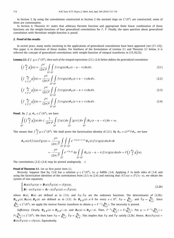

714 N.M. Tuan, N.T.T. Huyen / J. Math. Anal. Appl. 369 (2010) 712–718

In Section 3, by using the convolutions constructed in Section 2 the normed rings on L1(Rd) are constructed; some ofthem are commutative.

In Section 4, Theorem 4.1 states that arbitrary Hermite function and appropriate finite linear combination of thosefunctions are the weight-functions of four generalized convolutions for F , F̌ . Finally, the open question about generalizedconvolution with Hermitian weight-function is posed.

2. Proof of the results

In recent years, many works involving in the applications of generalized convolutions have been appeared (see [17–23]).This paper is in directions of those studies. For briefness of the formulation of Lemma 2.1 and Theorem 2.1 below, it isreferred the concept of generalized convolutions with weight-function of integral transforms in [15,18,23].

Lemma 2.1. If f , g ∈ L1(Rd), then each of the integral expressions (2.1)–(2.4) below defines the generalized convolution:(f

Φα∗F

g)(x) = i|α|

(2π)d

∫Rd

∫Rd

f (v)g(u)Φα(x − u − v)du dv, (2.1)

(f

Φα∗F ,F , F̌

g)(x) = i|α|

(2π)d

∫Rd

∫Rd

f (v)g(u)Φα(x + u − v)du dv, (2.2)

(f

Φα∗F , F̌ ,F

g)(x) = i|α|

(2π)d

∫Rd

∫Rd

f (v)g(u)Φα(x − u + v)du dv, (2.3)

(f

Φα∗F , F̌ , F̌

g)(x) = i|α|

(2π)d

∫Rd

∫Rd

f (v)g(u)Φα(x + u + v)du dv. (2.4)

Proof. By f , g,Φα ∈ L1(Rd), we have∫Rd

(f

Φα∗F

g)(x)dx � 1

(2π)d

∫Rd

∣∣ f (u)∣∣du

∫Rd

∣∣g(v)∣∣dv

∫Rd

∣∣Φα(x − u − v)∣∣dx < ∞.

This means that fΦα∗F

g ∈ L1(Rd). We shall prove the factorization identity of (2.1). By Φα = (i)|α| FΦα , we have

Φα(x)(F f )(x)(F g)(x) = i|α|

(2π)3d2

∫Rd

∫Rd

∫Rd

e−i〈x,u+v+t〉Φα(t) f (v)g(u)du dv dt

= i|α|

(2π)3d2

∫Rd

e−i〈x,y〉 dy

∫Rd

∫Rd

Φα(y − u − v) f (v)g(u)du dv = F(

fΦα∗F

g)(x).

The convolutions (2.2)–(2.4) may be proved analogously. �Proof of Theorem 1.1. Let us first prove item (i).

Necessity. Suppose that Eq. (1.4) has a solution ϕ ∈ L1(Rd), i.e. ϕ fulfills (1.4). Applying F to both sides of (1.4) andusing the factorization identities of the convolutions from (2.1) to (2.4) and noticing that (F f )(x) = ( F̌ f )(−x), we obtain thesystem of two equations{

A(x)(Fϕ)(x) + B(x)( F̌ϕ)(x) = (Fp)(x),

B(−x)(Fϕ)(x) + A(−x)( F̌ϕ)(x) = ( F̌ p)(x),(2.2b)

where A(x), B(x) are defined as in (1.5), and Fϕ, F̌ϕ are the unknown functions. The determinants of (2.2b):

D F , F̌ (x), D F (x), D F̌ (x) are defined as in (1.5). As D F , F̌ (x) �= 0 for every x ∈ Rd , Fϕ = D F

D F , F̌, and F̌ϕ = D F̌

D F , F̌. Since

D FD F , F̌

∈ L1(Rd), we apply the inverse Fourier transform to obtain ϕ = F −1( D FD F , F̌

). The necessity is proved.

Sufficiency. Clearly, D F , F̌ (x) ≡ D F , F̌ (−x), and D F (x) ≡ D F̌ (−x). Then, F −1( D FD F , F̌

) = F (D F̌

D F , F̌). Put ϕ := F −1( D F

D F , F̌) =

F (D F̌

D F , F̌) ∈ L1(Rd). We then have Fϕ = D F

D F , F̌, F̌ϕ = D F̌

D F , F̌. This implies that Fϕ and F̌ϕ satisfy (2.2b). Hence, A(x)(Fϕ)(x) +

B(x)( F̌ϕ)(x) = (Fp)(x). Equivalently,

N.M. Tuan, N.T.T. Huyen / J. Math. Anal. Appl. 369 (2010) 712–718 715

F

(λϕ(x) + i|α|

(2π)d

∫Rd

∫Rd

[k1(u)Φα(x − u − v) + k2(u)Φα(x + u − v)

+ k3(u)Φα(x − u + v) + k4(u)Φα(x + u + v)]ϕ(v)du dv

)= (Fp)(x).

By the inverse Fourier transform, ϕ fulfills (1.4) for almost every x ∈ Rd . Item (i) is proved.

Instead of the proof of item (ii), we shall prove the following claim.

Claim 2.1. Assume that λ �= 0. Then:

(i) D F , F̌ (x) �= 0 for every x outside a ball with finite radius.

(ii) If D F , F̌ (x) �= 0 ∀x ∈ Rd, and if Fp ∈ L1(Rd), then D F

D F , F̌∈ L1(Rd).

(i) By the Riemann–Lebesgue lemma, the function D F , F̌ is continuous on Rd and lim|x|→∞ D F , F̌ (x) = λ2 (see [24, Theo-

rem 7.5]). Now item (i) follows from λ �= 0 and the continuity of D F , F̌ .

(ii) By the continuity of D F , F̌ and lim|x|→∞ D F , F̌ (x) = λ2 �= 0, there exist R > 0, ε1 > 0 so that inf|x|>R |D F , F̌ (x)| > ε1.

Since the function D F , F̌ is continuous and not vanished in the compact set S(0, R) = {x ∈ Rd: |x| � R}, there exists ε2 > 0

so that inf|x|�R |D F , F̌ (x)| > ε2. We then have supx∈Rd1

|D F , F̌ (x)| � max{ 1ε1

, 1ε2

} < ∞. Hence, the function 1|D F , F̌ (x)| is continuous

and bounded on Rd . Note that the functions A, B are continuous and bounded on R

d . As Fp ∈ L1(Rd), each of two termsdefining D F as in (1.5) belongs to L1(Rd), i.e. D F ∈ L1(Rd). Due to the continuity and boundary of 1

|D F , F̌ (x)| , D FD F , F̌

∈ L1(Rd).

The claim is proved.The proof of Theorem 1.1 is complete. �

Remark 2.1. (a) In the general theory of integral equations, the requirement that D F , F̌ (x) �= 0 for every x ∈ Rd is the

normally solvable condition of the equation (see [12,13]). If λ �= 0, then the assumptions in item (ii) of Theorem 1.1 aresimpler and easier to check than that in item (i); these assumptions are well fair.

(b) If |α| = 0, then Φ0 is the Gaussian function. It is possible to prove that if k1,k2,k3,k4 are the Gaussian functions,so K (x, y) is. Many mathematical models of the problems in Physics, Medicine and Biology were constructed that reducedintegral equations with the Gaussian kernel (see [7–9,14]).

Put θ(x) = e−i〈x,h〉. We recall the theorem for proving Theorem 1.2.

Theorem 2.1. (See [6].) If f , g ∈ L1(Rd), then each one of the integral expressions from (2.5) to (2.8) defines the generalized convolu-tion: (

fθ∗F

g)(x) = 1

(2π)d2

∫Rn

f (x − y − h)g(y)dy, (2.5)

(f

θ∗F ,F , F̌

g)(x) = 1

(2π)d2

∫Rn

f (x + y − h)g(y)dy, (2.6)

(f

θ∗̌F

g)(x) = 1

(2π)d2

∫Rn

f (x − y + h)g(y)dy, (2.7)

(f

θ∗F̌ , F̌ ,F

g)(x) = 1

(2π)d2

∫Rn

f (x + y + h)g(y)dy. (2.8)

One interesting fact possessed by the factorization identities in this theorem is that the shift (or delay) h in the left-sidemoved only into the weight-function in the right-side. This is the main key for solving integral equations with differentshifts or delays.

Proof of Theorem 1.2. Note that the h in the convolutions (2.5)–(2.8) is separate. Therefore, by arguments similar to that inthe proof of item (i) in Theorem 1.1 we can prove easily item (i) of this theorem (see also [6]).

The assertion in the item (ii) of Theorem 1.2 is an immediate consequence of the following claim, the proof of which issimilar to that of Claim 2.1. �

716 N.M. Tuan, N.T.T. Huyen / J. Math. Anal. Appl. 369 (2010) 712–718

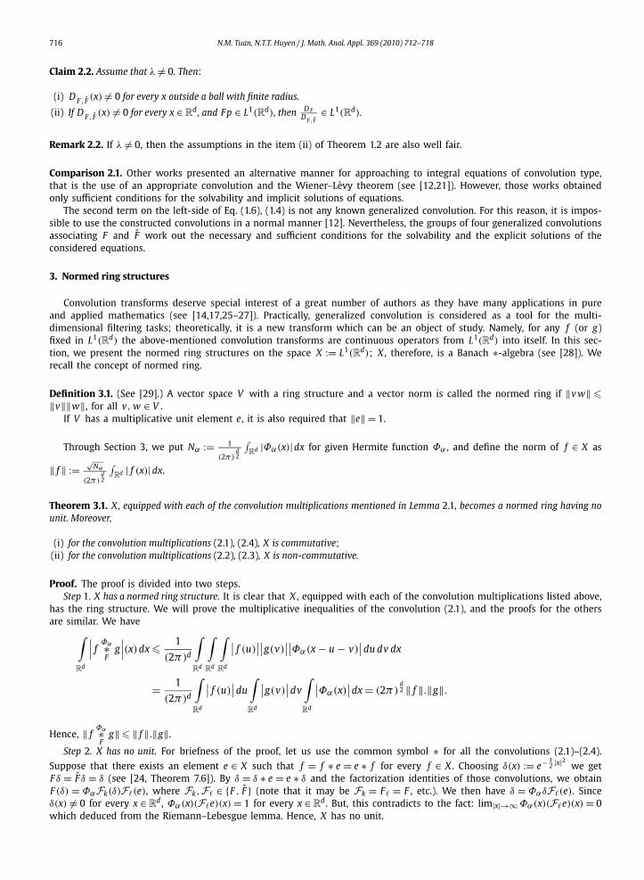
Claim 2.2. Assume that λ �= 0. Then:

(i) D F , F̌ (x) �= 0 for every x outside a ball with finite radius.

(ii) If D F , F̌ (x) �= 0 for every x ∈ Rd, and Fp ∈ L1(Rd), then D F

D F , F̌∈ L1(Rd).

Remark 2.2. If λ �= 0, then the assumptions in the item (ii) of Theorem 1.2 are also well fair.

Comparison 2.1. Other works presented an alternative manner for approaching to integral equations of convolution type,that is the use of an appropriate convolution and the Wiener–Lèvy theorem (see [12,21]). However, those works obtainedonly sufficient conditions for the solvability and implicit solutions of equations.

The second term on the left-side of Eq. (1.6), (1.4) is not any known generalized convolution. For this reason, it is impos-sible to use the constructed convolutions in a normal manner [12]. Nevertheless, the groups of four generalized convolutionsassociating F and F̌ work out the necessary and sufficient conditions for the solvability and the explicit solutions of theconsidered equations.

3. Normed ring structures

Convolution transforms deserve special interest of a great number of authors as they have many applications in pureand applied mathematics (see [14,17,25–27]). Practically, generalized convolution is considered as a tool for the multi-dimensional filtering tasks; theoretically, it is a new transform which can be an object of study. Namely, for any f (or g)fixed in L1(Rd) the above-mentioned convolution transforms are continuous operators from L1(Rd) into itself. In this sec-tion, we present the normed ring structures on the space X := L1(Rd); X , therefore, is a Banach ∗-algebra (see [28]). Werecall the concept of normed ring.

Definition 3.1. (See [29].) A vector space V with a ring structure and a vector norm is called the normed ring if ‖v w‖ �‖v‖‖w‖, for all v, w ∈ V .

If V has a multiplicative unit element e, it is also required that ‖e‖ = 1.

Through Section 3, we put Nα := 1

(2π)d2

∫Rd |Φα(x)|dx for given Hermite function Φα , and define the norm of f ∈ X as

‖ f ‖ :=√

Nα

(2π)d2

∫Rd | f (x)|dx.

Theorem 3.1. X, equipped with each of the convolution multiplications mentioned in Lemma 2.1, becomes a normed ring having nounit. Moreover,

(i) for the convolution multiplications (2.1), (2.4), X is commutative;(ii) for the convolution multiplications (2.2), (2.3), X is non-commutative.

Proof. The proof is divided into two steps.Step 1. X has a normed ring structure. It is clear that X , equipped with each of the convolution multiplications listed above,

has the ring structure. We will prove the multiplicative inequalities of the convolution (2.1), and the proofs for the othersare similar. We have∫

Rd

∣∣∣ fΦα∗F

g∣∣∣(x)dx � 1

(2π)d

∫Rd

∫Rd

∫Rd

∣∣ f (u)∣∣∣∣g(v)

∣∣∣∣Φα(x − u − v)∣∣du dv dx

= 1

(2π)d

∫Rd

∣∣ f (u)∣∣du

∫Rd

∣∣g(v)∣∣dv

∫Rd

∣∣Φα(x)∣∣dx = (2π)

d2 ‖ f ‖.‖g‖.

Hence, ‖ fΦα∗F

g‖ � ‖ f ‖.‖g‖.

Step 2. X has no unit. For briefness of the proof, let us use the common symbol ∗ for all the convolutions (2.1)–(2.4).

Suppose that there exists an element e ∈ X such that f = f ∗ e = e ∗ f for every f ∈ X . Choosing δ(x) := e− 12 |x|2 we get

F δ = F̌ δ = δ (see [24, Theorem 7.6]). By δ = δ ∗ e = e ∗ δ and the factorization identities of those convolutions, we obtainF (δ) = Φα Fk(δ)F(e), where Fk, F ∈ {F , F̌ } (note that it may be Fk = F = F , etc.). We then have δ = ΦαδF(e). Sinceδ(x) �= 0 for every x ∈ R

d , Φα(x)(Fe)(x) = 1 for every x ∈ Rd . But, this contradicts to the fact: lim|x|→∞ Φα(x)(Fe)(x) = 0

which deduced from the Riemann–Lebesgue lemma. Hence, X has no unit.

N.M. Tuan, N.T.T. Huyen / J. Math. Anal. Appl. 369 (2010) 712–718 717

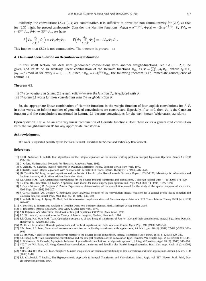
Evidently, the convolutions (2.2), (2.3) are commutative. It is sufficient to prove the non-commutativity for (2.2), as that

for (2.3) might be proved analogously. Consider the Hermite functions: Φ0(x) = e− 12 |x|2 , Φ1(x) = −2x1e− 1

2 |x|2 . By FΦα =(−i)|α|Φα , F̌Φα = (i)|α|Φα , we have

F(Φ0

Φα∗F ,F , F̌

Φ1

)= iΦαΦ0Φ1, F

(Φ1

Φα∗F ,F , F̌

Φ0

)= −iΦαΦ0Φ1.

This implies that (2.2) is not commutative. The theorem is proved. �4. Claim and open question on Hermitian weight-function

In this small section, we deal with generalized convolutions with another weight-functions. Let r ∈ {0,1,2,3} begiven, and let Ψ be an arbitrary linear combination of the Hermite functions Φαk as Ψ = ∑N

k=1 akΦαk , where ak ∈ C,|αk| = r (mod 4) for every k = 1, . . . , N . Since FΦαk = (−i)|αk|Φαk , the following theorem is an immediate consequence ofLemma 2.1.

Theorem 4.1.

(i) The convolutions in Lemma 2.1 remain valid whenever the function Φα is replaced with Ψ .(ii) Theorem 3.1 works for those convolutions with the weight-function Ψ .

So, the appropriate linear combination of Hermite functions is the weight-function of four explicit convolutions for F , F̌ .In other words, an infinite number of generalized convolutions are constructed. Especially, if |α| = 0, then Φ0 is the Gaussianfunction and the convolutions mentioned in Lemma 2.1 become convolutions for the well-known Weierstrass transform.

Open question. Let Ψ be an arbitrary linear combination of Hermite functions. Does there exists a generalized convolutionwith the weight-function Ψ for any appropriate transforms?

Acknowledgment

This work is supported partially by the Viet Nam National Foundation for Science and Technology Development.

References

[1] B.D.O. Anderson, T. Kailath, Fast algorithms for the integral equations of the inverse scatting problem, Integral Equations Operator Theory 1 (1978)132–136.

[2] G. Arfken, Mathematical Methods for Physicists, Academic Press, 1985.[3] K. Chanda, P.C. Sabatier, Inverse Problems in Quantum Scattering Theory, Springer-Verlag, New York, 1977.[4] T. Kailath, Some integral equations with “nonrational” kernels, IEEE Trans. Inform. Theory IT-12 (1966) 442–447.[5] J.N. Tsitsiklis, B.C. Levy, Integral equations and resolvents of Toeplitz plus Hankel kernels, Technical Report LIDS-P-1170, Laboratory for Information and

Decision Systems, M.I.T., silver edition, December 1981.[6] B.T. Giang, N.M. Tuan, Generalized convolutions for the Fourier integral transforms and applications, J. Siberian Federal Univ. 1 (4) (2008) 371–379.[7] P.S. Cho, H.G. Kuterdem, R.J. Marks, A spherical dose model for radio surgery plan optimization, Phys. Med. Biol. 43 (1998) 3145–3148.[8] F. Garcia-Vicente, J.M. Delgado, C. Peraza, Experimental determination of the convolution kernel for the study of the spatial response of a detector,

Med. Phys. 25 (1998) 202–207.[9] F. Garcia-Vicente, J.M. Delgado, C. Rodriguez, Exact analytical solution of the convolution integral equation for a general profile fitting function and

Gaussian detector kernel, Phys. Med. Biol. 45 (3) (2000) 645–650.[10] T. Kailath, B. Levy, L. Ljung, M. Morf, Fast time-invariant implementations of Gaussian signal detectors, IEEE Trans. Inform. Theory IT-24 (4) (1978)

469–477.[11] A. Böttcher, B. Silbermann, Analysis of Toeplitz Operators, Springer Monogr. Math., Springer-Verlag, Berlin, 2006.[12] H. Hochstadt, Integral Equations, John Wiley & Sons, New York, 1973.[13] A.D. Polyanin, A.V. Manzhirov, Handbook of Integral Equations, CRC Press, Boca Raton, 1998.[14] E.C. Titchmarsh, Introduction to the Theory of Fourier Integrals, Chelsea, New York, 1986.[15] B.T. Giang, N.V. Mau, N.M. Tuan, Operational properties of two integral transforms of Fourier type and their convolutions, Integral Equations Operator

Theory 65 (3) (2009) 363–386.[16] M. Rösler, Generalized Hermite polynomials and the heat equations for Dunkl operator, Comm. Math. Phys. 192 (1998) 519–542.[17] N.M. Tuan, P.D. Tuan, Generalized convolutions relative to the Hartley transforms with applications, Sci. Math. Jpn. 70 (1) (2009) 77–89 (e2009, 351–

363).[18] L.E. Britvina, A class of integral transforms related to the Fourier cosine convolution, Integral Transforms Spec. Funct. 16 (5–6) (2005) 379–389.[19] B.T. Giang, N.M. Tuan, Generalized convolutions and the integral equations of the convolution type, Complex Var. Elliptic Equ. 55 (4) (2010) 331–345.[20] B. Silbermann, O. Zabroda, Asymptotic behavior of generalized convolutions: an algebraic approach, J. Integral Equations Appl. 18 (2) (2006) 169–196.[21] N.X. Thao, V.K. Tuan, N.T. Hong, Generalized convolution transforms and Toeplitz plus Hankel integral equation, Fract. Calc. Appl. Anal. 11 (2) (2008)

153–174.[22] N.D.V. Nha, D.T. Duc, V.K. Tuan, Weighted lp -norm inequalities for various convolution type transformations and their applications, Armen. J. Math. 1 (4)

(2008) 1–18.[23] S.B. Yakubovich, Y. Luchko, The Hypergeometric Approach to Integral Transforms and Convolutions, Math. Appl., vol. 287, Kluwer Acad. Publ., Dor-

drecht/Boston/London, 1994.

718 N.M. Tuan, N.T.T. Huyen / J. Math. Anal. Appl. 369 (2010) 712–718

[24] W. Rudin, Functional Analysis, McGraw–Hill, New York, 1991.[25] B.T. Giang, N.M. Tuan, Generalized convolutions for the integral transforms of Fourier type and applications, Fract. Calc. Appl. Anal. 12 (3) (2009)

253–268.[26] H. Glaeske, V. Tuan, Mapping properties and composition structure of multidimensional integral transform, Math. Nachr. 152 (1991) 179–190.[27] Z. Tomovski, V.K. Tuan, On Fourier transforms and summation formulas of generalized Mathieu series, Math. Sci. Res. J. 13 (1) (2009) 1–10.[28] A.A. Kirillov, Elements of the Theory of Representations, Nauka, Moscow, 1972 (in Russian).[29] M.A. Naimark, Normed Rings, P. Noordhoff Ltd., Groningen, The Netherlands, 1959.