the sonar simulation toolset, release 4.1: science ... · the comprehensive acoustic system...
TRANSCRIPT
Applied Physics Laboratory University of Washington1013 NE 40th Street Seattle, Wash ing ton 98105-6698
The Sonar Simulation Toolset, Release 4.1:Science, Mathematics, and Algorithms
Technical Report
APL-UW TR 0404March 2005
Approved for public release; distribution is unlimited
by Robert P. Goddard
ONR Contracts N00014-01-G-0460 and N00014-98-G-0001
UNIVERSITY OF WASHINGTON • APPLIED PHYSICS LABORATORY
Acknowledgments
The Sonar Simulation Toolset was developed with sponsorship from several U. S. Navysources, most recently ONR Code 333 (Adam Nucci) and ONR’s “ARL Project”(Code 321US, John Tague). Earlier sponsors included the Naval Surface WarfareCenter, Carderock (William Beatty) and the Naval Underwater Systems Center, NewLondon, CT (Walter Hauck and Thomas Wheeler).
The SST development team at APL-UW consists of the author, Pete Brodsky,Patrick Tewson, Brandon Smith, and Don Percival. Warren Fox, Jim Luby, andChris Eggen have provided guidance, testing, and leadership. Earlier team mem-bers included Beth Kirby, Kou-Ying Moravan, Megan Hazen, Bill Kooiman, GordonBisset, and undergraduates Pat Lasswell and Jason Smith. Kou-Ying Moravan andPierre Mourad supplied the original Fortran implementations from which several ofthe boundary models started. Mike Boyd, Warren Fox, Greg Anderson, and ChrisEggen have contributed CASS expertise. The REVGEN project, where SST got itsstart, was led by Dave Princehouse.
The Comprehensive Acoustic System Simulation (CASS) program is availablethrough the support of the Naval Undersea Warfare Center, Newport (NUWCDI-VNPT). Permission to use and distribute CASS and GSM is granted by NUWC(Emily McCarthy).
SST’s users are the ingredients that make SST a useful tool instead of an aca-demic exercise. Special thanks are due to the many SST users at ARL/PSU andNUWC (Newport, RI), with whom we have enjoyed a long and fruitful collaborativerelationship.
Typeset August 20, 2004
ii TR 0404

UNIVERSITY OF WASHINGTON • APPLIED PHYSICS LABORATORY
Abstract
The Sonar Simulation Toolset (SST) is a computer program that produces simu-lated sonar signals, enabling users to build an artificial ocean that sounds like a realocean. Such signals are useful for designing new sonar systems, testing existing sonars,predicting performance, developing tactics, training operators and officers, planningexperiments, and interpreting measurements. SST’s simulated signals include rever-beration, target echoes, discrete sound sources, and background noise with specifiedspectra. Externally generated or measured signals can be added to the output sig-nal or used as transmissions. Eigenrays from the Generic Sonar Model (GSM) orthe Comprehensive Acoustic System Simulation (CASS) can be used, making all ofGSM’s propagation models and CASS’s Gaussian Ray Bundle (GRAB) propagationmodel available to the SST user. A command language controls a large collection ofcomponent models describing the ocean, sonars, noise sources, targets, and signals.The software runs on several different UNIX computers. The software runs on severalUNIX computers and Windows. SST’s primary documentation is the SST Web (alarge HTML “web site” distributed with the SST software), supported by a collectionof documented examples.
This report emphasizes the science, mathematics, and algorithms underlying SST.This report is intended to be updated often and distributed with SST as an integralpart of the SST documentation.
TR 0404 iii

UNIVERSITY OF WASHINGTON • APPLIED PHYSICS LABORATORY
Contents
Acknowledgments ii
Abstract iii
Contents iv
List of Figures vii
List of Tables viii
1 Introduction 1
1.1 Purpose . . . . . . . . . . . . . . . . . . . . . . . . . . . . . . . . . . 1
1.2 Objectives and Attributes . . . . . . . . . . . . . . . . . . . . . . . . 2
1.3 History . . . . . . . . . . . . . . . . . . . . . . . . . . . . . . . . . . . 3
1.4 Release . . . . . . . . . . . . . . . . . . . . . . . . . . . . . . . . . . . 5
1.5 Outline . . . . . . . . . . . . . . . . . . . . . . . . . . . . . . . . . . . 5
1.6 Notation . . . . . . . . . . . . . . . . . . . . . . . . . . . . . . . . . . 5
2 Overview 6
2.1 Assumptions . . . . . . . . . . . . . . . . . . . . . . . . . . . . . . . . 6
2.2 Outputs . . . . . . . . . . . . . . . . . . . . . . . . . . . . . . . . . . 7
2.3 Inputs . . . . . . . . . . . . . . . . . . . . . . . . . . . . . . . . . . . 7
2.4 Models . . . . . . . . . . . . . . . . . . . . . . . . . . . . . . . . . . . 8
2.5 Units and Coordinate Systems . . . . . . . . . . . . . . . . . . . . . . 10
2.6 Computers . . . . . . . . . . . . . . . . . . . . . . . . . . . . . . . . . 11
3 Example 12
4 Signals and Signal Transformations 13
4.1 Signal Representations . . . . . . . . . . . . . . . . . . . . . . . . . . 13
4.1.1 Real Samples . . . . . . . . . . . . . . . . . . . . . . . . . . . 13
4.1.2 Complex Envelope . . . . . . . . . . . . . . . . . . . . . . . . 14
4.1.3 Windowed Frequency Domain . . . . . . . . . . . . . . . . . . 15
4.2 Second Moment Time Series: Power Spectra and Scattering Functions 16
4.2.1 Power Spectra . . . . . . . . . . . . . . . . . . . . . . . . . . . 16
4.2.2 Scattering Functions . . . . . . . . . . . . . . . . . . . . . . . 18
iv TR 0404

UNIVERSITY OF WASHINGTON • APPLIED PHYSICS LABORATORY
4.3 Data Flow Design . . . . . . . . . . . . . . . . . . . . . . . . . . . . . 18
4.4 Data Flow Classes . . . . . . . . . . . . . . . . . . . . . . . . . . . . 22
4.5 Basic Signal Operations . . . . . . . . . . . . . . . . . . . . . . . . . 24
4.5.1 Variable Delays . . . . . . . . . . . . . . . . . . . . . . . . . . 25
4.5.2 Variable Finite Impulse Response Filters . . . . . . . . . . . . 27
4.6 Generating Signals . . . . . . . . . . . . . . . . . . . . . . . . . . . . 28
4.6.1 Generating Gaussian Noise . . . . . . . . . . . . . . . . . . . . 28
4.6.2 Generating Harmonic Tone Families . . . . . . . . . . . . . . . 30
4.6.3 Generating Modulated Tones . . . . . . . . . . . . . . . . . . 30
4.7 Window Functions . . . . . . . . . . . . . . . . . . . . . . . . . . . . 31
4.8 Grids . . . . . . . . . . . . . . . . . . . . . . . . . . . . . . . . . . . . 32
5 The Eigenray Model 33
5.1 Straight-line Eigenray Model . . . . . . . . . . . . . . . . . . . . . . . 35
5.2 CASS/GRAB Eigenrays . . . . . . . . . . . . . . . . . . . . . . . . . 37
5.3 Generic Sonar Model (GSM) Eigenrays . . . . . . . . . . . . . . . . . 37
5.4 Eigenray Interpolation and Ray Identity . . . . . . . . . . . . . . . . 38
6 Ocean Model 39
6.1 Ocean Depth . . . . . . . . . . . . . . . . . . . . . . . . . . . . . . . 39
6.2 Ocean Sound Speed . . . . . . . . . . . . . . . . . . . . . . . . . . . . 40
6.3 Ocean Volume Attenuation . . . . . . . . . . . . . . . . . . . . . . . . 40
6.4 Surface and Bottom Models . . . . . . . . . . . . . . . . . . . . . . . 40
6.4.1 Reflection Coefficients . . . . . . . . . . . . . . . . . . . . . . 41
6.4.2 Bistatic Scattering Strength . . . . . . . . . . . . . . . . . . . 42
6.4.3 Boundary Classes . . . . . . . . . . . . . . . . . . . . . . . . . 42
6.5 Volume Scattering Strength . . . . . . . . . . . . . . . . . . . . . . . 43
7 Sonar and Source Models 44
7.1 Trajectories and Coordinate Transformations . . . . . . . . . . . . . . 45
7.2 Beam Patterns . . . . . . . . . . . . . . . . . . . . . . . . . . . . . . 46
7.3 Sonar Transformation . . . . . . . . . . . . . . . . . . . . . . . . . . . 48
7.4 Source Transformation . . . . . . . . . . . . . . . . . . . . . . . . . . 48
8 Direct Sound Propagation Models 49
8.1 DirectSignal . . . . . . . . . . . . . . . . . . . . . . . . . . . . . . . . 50
8.2 DirectSpectrum . . . . . . . . . . . . . . . . . . . . . . . . . . . . . . 50
TR 0404 v

UNIVERSITY OF WASHINGTON • APPLIED PHYSICS LABORATORY
9 Target Echo Model 51
9.1 Target Models . . . . . . . . . . . . . . . . . . . . . . . . . . . . . . . 52
9.1.1 PointTarget . . . . . . . . . . . . . . . . . . . . . . . . . . . . 52
9.1.2 HighlightTarget . . . . . . . . . . . . . . . . . . . . . . . . . . 53
9.1.3 ExternalTarget . . . . . . . . . . . . . . . . . . . . . . . . . . 53
10 Reverberation 54
10.1 Generating Reverberation . . . . . . . . . . . . . . . . . . . . . . . . 55
10.2 Computing the Scattering Function . . . . . . . . . . . . . . . . . . . 56
11 Summary and Plans 58
REFERENCES 61
vi TR 0404

UNIVERSITY OF WASHINGTON • APPLIED PHYSICS LABORATORY
List of Figures
1 SST Component Models . . . . . . . . . . . . . . . . . . . . . . . . . 8
2 Total Signal for Pursuit Example . . . . . . . . . . . . . . . . . . . . 11
TR 0404 vii

UNIVERSITY OF WASHINGTON • APPLIED PHYSICS LABORATORY
List of Tables
1 Signal Classes . . . . . . . . . . . . . . . . . . . . . . . . . . . . . . . 22
2 Spectrum Classes . . . . . . . . . . . . . . . . . . . . . . . . . . . . . 23
3 Scattering Function Classes . . . . . . . . . . . . . . . . . . . . . . . 23
4 Window Function Classes . . . . . . . . . . . . . . . . . . . . . . . . 32
5 Surface and Bottom Models . . . . . . . . . . . . . . . . . . . . . . . 43
6 Beam Pattern Models . . . . . . . . . . . . . . . . . . . . . . . . . . . 47
viii TR 0404
UNIVERSITY OF WASHINGTON • APPLIED PHYSICS LABORATORY
1 Introduction
1.1 Purpose
The Sonar Simulation Toolset (SST) is a computer program that produces simulatedsonar signals as “heard” by a user-specified active or passive sonar in a user-specifiedocean environment. It enables a user to create an “artificial ocean” that may be usedto test new or proposed sonar systems or tactics, to train sonar operators, to planexperiments, or to validate models of underwater acoustic phenomena by comparingsimulation results with measurements.
This paper focuses on the science, mathematics, and algorithms used in SST. It isintended, in part, as a tutorial to introduce scientists and engineers to the technicalissues that must be addressed by any sonar signal simulation system. It is alsointended as a supplement to the existing SST documentation, adding informationon “how it works” and “why” to the existing descriptions of “how to do it”. Andit is intended to help scientists, engineers, trainers, and technical managers decidewhether SST might be useful in their projects.
This report started as an on-line, extended version of a paper for the classified USNavy Journal of Underwater Acoustics. To enable wider distribution, that paper’ssensitive “Applications” section is omitted here. Because it is intended to be used asan integral part of the SST documentation, this report contains software-specific de-tails that were omitted from the JUA version. It contains several features to enhanceon-line browsing, including active (click-through) references to equations, figures, re-lated text sections, and citations. This report will be updated often as the softwarechanges.
A separate on-line document, the SST Web [SST Web], gives details about how touse SST. It includes working examples of SST simulations for several different kinds ofactive and passive sonar systems. Yet another on-line document, which is generatedfrom the source code and comments therein using the Doxygen [Doxygen] software,covers the internal design of SST.
The SST software, together with all of the documentation just mentioned (in-cluding this report), are delivered to DoD agencies and contractors via a secure Website [APL SBU].
We will assume that the reader is familiar with underwater sound at the levelof [Urick 1983], and with digital sonar processing at the level of Knight et al. [Knight
TR 0404 1
UNIVERSITY OF WASHINGTON • APPLIED PHYSICS LABORATORY
1981]. It will be helpful, but not required, for the reader to be familiar with discrete-time signal processing [Oppenheim Schafer 1989] and the fundamentals of object-oriented software design [Page-Jones 2000].
1.2 Objectives and Attributes
SST is certainly not the only sonar simulation system available to the Navy commu-nity. It may or may not be appropriate for a given application, depending on thepurpose of the simulation. General modeling tools like CASS [Weinberg et al. 2001]or SWAT [Sammelmann 2002], real-time simulators like WAF [Correia 1988, Katyl2000], tactical simulators like TRM, or application-specific tools may have a place ina simulation tool kit. To understand where SST fits, consider the following objectivesand attributes of SST:
Signal Level Simulation: SST produces sound, suitable as input for users’ ears,for the front end of a sonar system, or for a computer model of an existing orproposed sonar front end. It does not produce plots or predict performance byitself.
Portable: SST is designed to run on nearly any modern general-purpose computer.Each distribution includes pre-built versions for SPARC/Solaris, Intel/Linux,and Intel/Windows/Cygwin [Cygwin] systems, plus source code and portingtools to make it as easy as possible to port it to other systems.
General: SST is suitable for simulating a wide variety of active or passive sonarsystems, sound sources, and targets in many different environments and scenar-ios. Multiple sound sources, multiple targets, complicated sonar systems andsignals, arbitrary trajectories, variable bathymetry, various surface and bottommodels, and many other details can be specified using SST’s flexible commandlanguage.
Broadband: SST is suitable for signals of any bandwidth. The frequency range islimited primarily by its ray-based propagation models, which can be useful aslow as a few kHz in shallow water or even lower in deep water, depending onthe requirement for fidelity.
Multistatic: There can be any number of sound sources, receivers, and targets onany number of platforms.
Multi-channel: The sonar can have any number of channels, each of which is char-acterized by its own sensitivity pattern and offset. A channel may represent the
2 TR 0404

UNIVERSITY OF WASHINGTON • APPLIED PHYSICS LABORATORY
signal behind one transducer (element-level) or for one beam behind the beamformer (beam-level). Correlations between channels are carefully controlled.
Non-Real-Time: SST is not constrained to run in real time.
Flexible Fidelity: SST’s lack of real-time constraint allows the user to trade offspeed for fidelity and detail, striking whatever balance is consistent with theuser’s requirements, budget, and patience. The idea is to support whateverlevel of fidelity and detail is required for each application, without unnecessarilyslowing the simpler simulations. The level of realism can, if necessary, be quitehigh, and simple simulations can achieve much faster than real-time throughput.
Embeddable: SST may be used as a signal generation component within a higher-level simulation. It is being used that way within TRM at ARL-PSU.
Streamable: SST’s results are produced in time order. The early parts of the outputare written as soon as possible, usually well before the simulation is finished.This feature is essential for embedded applications and for parallel processing(currently in development), and it helps minimize memory requirements forlong runs. Another advantage is that users can examine partial results beforedeciding whether to continue a long simulation run.
Object Oriented: SST’s command language, its primary implementation language(C++), and SST’s design are organized around the concepts of objects, classes,encapsulation, inheritance, and polymorphism. The advantages of this approachare documented in standard software engineering texts [Page-Jones 2000].
Unclassified: SST’s distribution is limited to DoD and DoD contractors only (crit-ical technology), but the code and documentation are not classified.
1.3 History
Most of the support for SST’s development has come through projects supportingspecific applications. Hence SST’s current capabilities reflect, to a dominant degree,the union of the requirements specified for those applications. In response to changingrequirements, innovations were introduced in roughly the following order:
• SST’s roots trace back to the REVGEN (Reverberation Generator) [Princehouse1975,Princehouse 1978,Goddard 1986] project of the 1970s and early 1980s. SSTitself started in 1989. The focus was on high-frequency, narrow-band, monos-tatic active sonar systems. The initial few versions generated reverberation andtarget echoes using a narrow-band point scatterer model (Sec. 10).
TR 0404 3
UNIVERSITY OF WASHINGTON • APPLIED PHYSICS LABORATORY
• In the early 1990s the emphasis shifted to broadband sonars. This led to up-dated high-frequency environmental models [APL Models 1994], an optionalscattering-function reverberation model [Luby Lytle 1987], frequency-dependentenvironmental models and beam patterns, and the “data flow” architecture(Sec. 4.3).
• Another thrust during the middle 1990s was toward multistatic operation.SST’s monostatic reverberation models were replaced by a fully bistatic, broad-band one based on scattering functions (Sec. 10). Bistatic surface and bottommodels were also introduced (Sec. 6).
• During this period, both the number of SST users and the size and complexityof the code rose dramatically. In response, we replaced the earlier text docu-mentation with an extensively cross-linked HTML Web version [SST Web], andC++ replaced C as the primary programming language.
• Starting in 1997 several applications involved frequencies below 10 kHz. Thisled to a new mid-frequency bistatic surface model [Gilbert 1993], an upgradedbottom model, an external target model (Sec. 9.1.3), and better support forpassive sonars.
• The Navy’s concern shifted from deep water to littoral environments. In re-sponse, we added support in SST for range-dependent propagation using eigen-rays computed using the GRAB [Weinberg Keenan 1996] eigenray model.
• In broadband, shallow-water applications, SST users recognized that the pro-cessing gain for simulated target echoes versus reverberation and countermea-sures was too optimistic. The main culprit was identified as near-specular scat-tering from the surface and bottom. In response, we added time and frequencyspreading (reduced coherence in frequency and time) (Sec. 11).
• Several users wanted to use SST as a signal generation component in a higher-level tactical simulation. Other users wanted to use some of SST’s models inother environments. These requirements have led to a continuing push towardinteroperability.
• Current efforts, driven by user concerns, include improved coherence control,faster element-level simulations for systems with a very large number of hy-drophones, user interface support for combined active and passive processing,ship wakes, very long active transmissions, and better realism at lower frequen-cies.
• Everyone always wants more speed, better documentation, fewer software er-rors, a simpler and more intuitive user interface, more checks to prevent user
4 TR 0404

UNIVERSITY OF WASHINGTON • APPLIED PHYSICS LABORATORY
mistakes, interoperability with other systems, and more and better support forusers. We are constantly working to improve SST and our services in all ofthese measures.
SST has played a significant role in many studies over the years. Unclassifiedpublished ones include [Eggen Goddard 2002], [Goddard 2000], and [Rouseff et al.2001].
1.4 Release
The version of SST described here is Release 4.1, dated November 2002.
1.5 Outline
Section 2 is a general overview of SST and its component models. Section 3 presentsa simple example showing the results of an SST simulation. The bulk of the paperdescribes the science and mathematics underlying SST. The order in which SST’svarious sub-models are described is intended to support linear reading by placingthe background needed to understand a model’s requirements before that model’sdescription. We conclude, in Section 11, with a brief description of current andplanned projects to improve SST’s realism, scope, and ease of use.
1.6 Notation
In nearly all of this paper, we treat the signals, transformations, and models ascontinuous in time, space, frequency, and direction. This is a physicist’s point of view,not a software engineer’s. Of course, as in any digital implementation, conceptuallycontinuous functions are sampled at discrete values of their independent variables,and integrations are implemented as finite sums, and precision is limited. We discussdigital samples when it is necessary to do so. In our view, however, the physicaland mathematical concepts are easier to understand in the continuous domain, sowe remain there whenever possible. The mapping between continuous and digitaldomains is covered well by standard texts [Oppenheim Schafer 1989,Hamming 1973].
SST is object oriented on two levels, the SST command language and the imple-mentation language. For the most part, an SST input file consists of statements thatdefine objects that are instances of built-in SST classes, and assign values to named
TR 0404 5
UNIVERSITY OF WASHINGTON • APPLIED PHYSICS LABORATORY
attributes (parameters) of those objects. Each of the classes visible through thecommand language is implemented in terms of a C++ class having the same name,with attributes corresponding to C++ member variables. We do not distinguish herebetween the two kinds of classes.
Within paragraph text, class names are displayed in bold sans serif font andcapitalized; examples are Signal, PistonBeam, and JacksonBottom. Names of classattributes are displayed in slanted sans serif font and uncapitalized; examples arefrequency , radius, and soundSpeedRatio.
2 Overview
2.1 Assumptions
The simulated sound produced by SST consists of a digital representation of thepredicted signal in each channel of the sonar receiver’s processing path. This soundmay contain components from four types of sources:
Discrete sound sources: “Passive targets,” such as ships or countermeasures, thatradiate noise from a compact region
Diffuse sound sources: Environmental noise and self noise
Discrete scatterers: “Active targets,” such as submarines or rocks, that echo anactive sonar’s transmitted pulses (or other sound) back to the sonar receiver
Reverberation: Diffuse scatterers, such as the ocean bottom, that send back manyoverlapping echoes of an active sonar’s pulse
The sonar system can be passive (receiver only), or it can be active (listening forechoes of its own transmissions). Active sonars can be monostatic (transmitter andreceiver on the same platform), bistatic (transmitter and receiver on two differentplatforms), or multistatic (employing several transmitters or receivers).
The receiver can have any number of channels (transducers or beams). Therecan be any number of sound sources and targets, and any number of sound paths(eigenrays) connecting sources, scatterers, and receivers. For both passive and activesonars, the signals can have an arbitrarily wide range of frequencies. The ocean,sound scatterers, and beam patterns act as filters that alter the frequency content of
6 TR 0404

UNIVERSITY OF WASHINGTON • APPLIED PHYSICS LABORATORY
the sound. Transmissions and listening intervals can be arbitrarily long. Of course,all of these parameters will have an impact on size and speed, so the practical limitsdepend on available disk space, memory, processor speed, and the patience of theuser.
Over the last decade, SST’s most active users (and most of its financial support)have come from the torpedo development community. Therefore, its high-frequencyenvironmental models are more complete and up-to-date than its lower-frequencymodels. The current propagation models are based on eigenrays, not on direct solu-tions of the wave equation. These factors limit the realism of SST’s simulations forlow frequencies, especially in shallow water.
2.2 Outputs
SST’s primary output is multi-channel sampled sound: a digital representation ofthe simulated signal somewhere in the sonar receiver. A channel can represent eitherthe signal behind a transducer (for element-level simulations) or an output of thebeamformer (for beam-level simulations).
SST can also produce several other types of data, including the reverberation scat-tering function, various types of spectra and cross-spectra, and synthesized signalsintended for use as transmissions or noise sources. Some of these are intermediateproducts used in the simulation, and some result from general-purpose signal process-ing tools (like a spectrum analyzer) that the user can apply to any signal.
These simulated signals and related data can be written into an external file inany of several user-specified forms, binary or text. Any of these forms can be readby SST as well as written. The ways that SST can represent or store signals aredescribed in Sec. 4.
SST does not produce plots or other displays. Post-run analysis and plotting canbe done using commercial packages like Mathematica [Mathematica] or Matlab [Mat-lab], or public-domain tools like Octave [Octave] or Gnuplot [Gnuplot], specializedtools like the SIO package from Scripps [Hodgkiss 1989], or many other tools. A largeand growing set of useful Matlab scripts are provided with SST.
2.3 Inputs
The primary inputs to an SST simulation consist of commands for generating thevarious types of signals, plus assignment statements in which the user specifies the
TR 0404 7

UNIVERSITY OF WASHINGTON • APPLIED PHYSICS LABORATORY
Figure 1: SST Component Models
Ocean
SoundSpeed
Absorption
BoundaryReflection
Scattering
Sonar Transmitter
Trajectory
Beam(freq)
Signal
T
Sonar Receiver
Beam(freq)
R
RTrajectory Signal
Eigenray
delay, loss(freq), directions
Target
Trajectoryhighlights
Source
TrajectorySignalBeam
Filters, Delays
Reverberation
Target Echo
One-way Signal
GenerateBroadband Noise
Spectra
Any External Signal
Bathymetry
characteristics of the ocean environment, the sonar transmitter and receiver, activeand passive targets, and the format of the simulated signal. These specifications andcommands are expressed in a simple but flexible language with an object-orientedflavor reminiscent of Python or C++. They may be entered from the keyboard,read from text files, or passed via a pipe from a higher-level program. The languagesupports user-defined variables and comments to help make the scripts readable.
Signals used as transmissions or noise sources can come from external files havingthe same file formats as SST’s outputs. SST also includes tools for specifying andgenerating these signals internally (Sec. 4.6).
Eigenrays and beam patterns can come from external files, text or binary.
2.4 Models
SST is based on a large number of underlying models — mathematical representationsof physical phenomena — which specify how each element of the environment affectsthe sound. Figure 1 summarizes those component models and the relationships amongthem.
8 TR 0404
UNIVERSITY OF WASHINGTON • APPLIED PHYSICS LABORATORY
Eigenray Model: SST’s sound propagation models are based on eigenrays —paths through the water along which sound propagates between two specified end-points. Sound in the neighborhood of a receiver or scatterer is a sum of copies of theoriginal transmitted sound, each of which arrives at a different time from a differentdirection, and each of which has been attenuated in a frequency-dependent way. SSTprovides three choices (plus variants) for eigenray models: a straight-line model withreflections (the base class), one based on eigenrays from the GRAB eigenray modelin the CASS software, and one based on any of several eigenray models provided bythe GSM software. The eigenray models are discussed in Sec. 5.
Ocean Model: The SST user specifies the ocean environment by describingcharacteristics of the surface and bottom, the depth, the volume scattering strength,and the sound speed and absorption rate of the water itself. These models act asinputs to the eigenray model and the reverberation model. The various componentsof the ocean model are discussed in Sec. 6.
Sonar and Source Models: The sonar receiver is specified by giving its trajec-tory through the water, the location of each channel’s phase center, and the beampattern giving each channel’s sensitivity versus direction and frequency. Each discretesound source is described in terms of its trajectory, the signal it transmits, and thedirectional behavior of the transmission (beam patterns). An active sonar’s transmit-ter is treated just like any other sound source; hence the “Sonar Transmitter” modelin Fig. 1 is the same as the “Source” model. These models are discussed in Sec. 7.
Target Model: Each target (for active sonars) is an object (with a trajectory)that receives a signal from a source and re-transmits it to a sonar; hence it acts like agroup of receivers and sources back to back. Several target models are available; eachone provides a different way to specify the relationship between the received soundand the re-transmitted sound. The current target models describe that relationshipin terms of highlights. They are described in Sec. 9.1.
Direct (One-way) Sound Propagation: The heavy arrows in Fig. 1 representthe various ways that a source signal is transformed on its way to being received bya sonar system. The simplest one, marked “One-way Signal” on the diagram, is alsocalled “direct” sound propagation. This transformation combines properties of thesource model, the eigenray model, and the sonar model, and reduces them to a set offilters and delays that transform the signal emitted by a source into the signal receivedby a sonar via paths that may involve reflection and refraction but not scattering.This transformation is described in Sec. 8.
Target Echoes: The heavy arrows in Fig. 1 marked “Target Echo” representsound that scatters from a discrete target. It is essentially two “one-way signals” inseries, with the target model in between. This transformation is described in Sec. 9.
TR 0404 9

UNIVERSITY OF WASHINGTON • APPLIED PHYSICS LABORATORY
Reverberation: The heavy arrows in Fig. 1 marked “Reverberation” representsound that scatters from a very large number of very small scatterers distributedthroughout the environment. This is conceptually very similar to a lot of targetechoes, but SST treats them statistically, so the implementation of the transformationis quite different from target echoes. Reverberation is described in Sec. 10.
Noise and Other Sound: Sound from any source can be added to SST’s one-way signals, target echoes, and reverberation. SST can produce broadband Gaussiannoise having a user-specified power spectrum, as described in Sec. 4.6.1; this type ofnoise is useful to represent ambient noise, self-noise, and electronic noise. BroadbandGaussian noise can also be used as the emission from any sound source, for which itmay be combined with harmonic families of tones or active transmit pulses. Signalsfor any of these purposes may be generated internally by SST, or read in from anexternally generated file.
Signal Processing: All of the signal transformations are built on top of a di-verse set of general-purpose signal processing tools for generating, summing, filtering,delaying, scaling, Fourier analyzing, and otherwise transforming signals. All of thesesignal processing tools can be hooked together like plumbing, or they can be used sep-arately. The “data flow” architecture that makes this flexibility possible is describedin Sec. 4.3, and the components themselves are described in Sec. 4.4.
2.5 Units and Coordinate Systems
In SST and in this paper, acoustic pressure is expressed in micro-Pascals (µPa),acoustic intensity is in µPa2 or in dB//µPa2, and angles are in degrees. All othermeasurements are expressed in MKS units.
In the Earth-centered coordinate system, vector components are in the order(North, East, Down) with an origin at an arbitrary point on the surface of the ocean.Earth curvature is ignored, except insofar as it is included in the CASS and GSMeigenray models (Sec. 5). In platform-centered coordinate systems (used for beampatterns, element offsets, and target highlights), vector components are in the order(Forward, Starboard, Below) relative to an arbitrary origin on the platform (sonar,source, or target). The mapping between the two types of coordinate systems isdefined by the trajectory attribute of the vehicle, as described in Sec. 7.1.
10 TR 0404

UNIVERSITY OF WASHINGTON • APPLIED PHYSICS LABORATORY
Figure 2: Total Signal for Pursuit Example
Tim
e (s
)
Frequency (kHz)
Total Signal, Ping 1
29 29.5 30 30.5
0.5
1
1.5
2
2.5
3 10
20
30
40
50
60
70
80
40 60 80 100
0.5
1
1.5
2
2.5
3
Level (dB // uPa2)
2.6 Computers
This release of SST has been tested on SPARC/Solaris and Intel/Linux computers.An Intel/Windows port under the Cygwin [Cygwin] environment is planned. SST isdesigned to be portable, and previous versions of SST have been ported to severalother UNIX-like systems.
TR 0404 11

UNIVERSITY OF WASHINGTON • APPLIED PHYSICS LABORATORY
3 Example
Figure 2 is a Matlab display showing the result of SST’s “Pursuit” example, whichis one of the standard examples provided with SST. The Pursuit scenario featuresa monostatic, high-speed, torpedo-like active sonar chasing after a submarine-liketarget. SST produced the multi-channel signal heard by the sonar, which includesthe target echo, reverberation, and noise produced by the fleeing target. The Matlabscripts that produced the figure sliced that signal into short segments, computedthe power spectral density for each segment, and displayed the results, both as atime-dependent spectrum and as total signal level.
The dominant feature in the figure is the reverberation, which comes primarilyfrom the surface in this scenario. The early part of the signal comes from almostdirectly overhead, via the sidelobes of the beam pattern; hence it has very littleDoppler shift. The later part of the reverberation comes from the main lobe, almoststraight ahead; hence it has a high upward Doppler shift (the main ridge down themiddle of the spectrum). This obvious “reverberation hook” from low early Dopplerto high late Doppler is characteristic of forward-looking sonars. Less obvious is thestreak that starts at about 0.9 seconds and merges with the main ridge; that comesfrom a path that reflects from the bottom.
The target echo is the blip just after 1.0 second and just above 29.5 kHz. It hasa lower Doppler shift than the main reverberation ridge because it is running away.This is an “easy” high-Doppler detection despite the fact that the level of the targetreturn is well below the level of the reverberation (the target doesn’t show at all onthe level plot on the right).
Note that this is a very simple analysis of a very simple scenario. Only one channelis shown (although the receiver in the example has 5 channels); complications likeinter-channel correlations are in the SST-generated signal but not shown by thisanalysis. The pulse is a narrow-band pure tone, so the Fourier analysis used here isnearly optimal; a broadband pulse would require more complex analysis, probablyfeaturing replica correlation. The sonar is monostatic, and only a few eigenrays aresignificant. These limitations are not imposed by SST, which can support much morecomplicated scenarios requiring much more complicated processing, both by SST andby the post-processing algorithms needed to analyze the results.
The SST script for this example can run in a few seconds on a modern workstation— close to real-time throughput (but not real-time in terms of response deadlines).More complicated scenarios would take more time.
12 TR 0404

UNIVERSITY OF WASHINGTON • APPLIED PHYSICS LABORATORY
4 Signals and Signal Transformations
The inputs, outputs, and much of the intermediate data of SST consist of signals.In this section we address the question, “What is a signal?” from several points ofview, including abstract meaning, sampled representations, and software components.These issues are addressed early because they form the scaffolding on which much ofthe SST system is built.
4.1 Signal Representations
Conceptually, a signal xc(t) is a continuous, band-limited, multi-channel function oftime t, with channels indexed by c. A signal may represent (for example) voltage ona set of wires or sound pressure at a set of locations in the water. Within SST eachsignal is represented as a sequence of sets of sample values xc(tn) corresponding todiscrete values tn of the time. SST supports three distinct, equivalent representationsof a signal: real samples, complex envelope, and windowed frequency domain. Allsignals in SST, whether they are used for input, output, or in between, are representedin one of these three ways.
4.1.1 Real Samples
The most straightforward way to represent a real signal xc(t) in SST is as a sequenceof real samples on a uniform grid of time values:
xc(tn) = xc(t0 + nh), (1)
where n is an integer and h is the time increment between samples.
If the Fourier transform of the original continuous signal xc(t) is negligible forfrequencies greater than some maximum frequency Fmax, and the sample interval his chosen such that Fmax is within the Nyquist band:
h < 1/(2Fmax), (2)
then the original signal can be recovered (in principle) using band-limited interpola-tion:
xc(t) =∞∑
n=−∞
(sin(π(t− tn)/h)
π(t− tn)/h
)xc(tn). (3)
TR 0404 13

UNIVERSITY OF WASHINGTON • APPLIED PHYSICS LABORATORY
The problematic infinities and long decay time of this equation will be dealt with inSection 4.5.1, when we describe the delay algorithm.
SST Class: The base class from which all time-domain signals are derived isSignal, which has attributes frequency , isComplex , and times. To specify the realsample representation in any class derived from Signal, set isComplex to false andtimes to a UniformGrid specifying the sample times. More details about this familyof classes will be given in the subsections 4.3 and 4.4 below.
4.1.2 Complex Envelope
For a band-limited signal, a bandwidth W and a center frequency F exist such thatthe Fourier transform of the signal is negligibly small outside the frequency rangeFmin = F − W/2 to Fmax = F + W/2. If W is sufficiently small compared to F , itis often advantageous to express such signals in complex envelope notation [Knight1981]. The real-valued signal xc(t) is expressed in terms of a complex envelope xc(t):
xc(t) =√
2<(xc(t) e2πiFt
). (4)
The inverse transformation is (ideally)
xc(t) =√
2[xc(t) e−2πiFt
]LP
, (5)
where <() denotes the real part of a complex number, and the subscript LP denotesapplication of an ideal low-pass filter with a passband of −W/2 to W/2 and unitygain. The complex envelope xc(t) is advantageous because it varies much more slowlywith time than does the real signal xc(t) (to the extent that W � F ). The complexenvelope may be sampled and interpolated using Eq. (3) just like the original realsignal, but now the maximum sample interval h required to fully recover the signal isdetermined by the bandwidth, not the maximum frequency Fmax:
h ≤ 1/W, (6)
i.e., the Nyquist band extends from F − 1/(2h) to F + 1/(2h). As a general rule,the complex envelope notation is advantageous whenever the ratio of bandwidth tomaximum frequency is less than about 25%.
Normalization: The constant√
2 in Eqs. (4) and (5) is chosen to preserve power:Av {|xc(t)|2} = Av {[xc(t)]
2}, where Av {} denotes a time average.
SST Class: To specify the complex envelope representation in any class derivedfrom the base class Signal, set frequency to the center frequency F , isComplex to true,and times to a UniformGrid specifying the sample times.
14 TR 0404

UNIVERSITY OF WASHINGTON • APPLIED PHYSICS LABORATORY
SST Class: Transformations between real samples and complex envelope samplesare implemented in SST class ResampleSignal, which uses approximate forms ofEqs. (4) and (5) employing window functions to combine finite-length filters withfinite-order interpolation.
4.1.3 Windowed Frequency Domain
The third signal representation used in SST is a windowed frequency domain form.Currently, the primary application for the windowed frequency domain representationis in the implementation of class DirectSpectrum, which will be discussed in Sec. 8.
Conceptually, we break the continuous signal into blocks of a convenient size (oneper update cycle) and perform a Fourier transform on each block. To avoid end effects,we enlarge the blocks so that they overlap, and multiply each one by a smooth “pre-window function” w(t) whose properties are specified below. The transformationstarting from a continuous signal is
Xc(f, tu) =
∫ ∞
−∞w(t− tu) xc(t) e−2πif(t−tu) dt, (7)
where the index u labels an update time on a uniform grid with interval ∆:
tu = t0 + u∆. (8)
Note that the update interval ∆ is normally much larger than the signal samplingfrequency h used in Eq. (1).
The inverse operation, from windowed frequency domain to continuous signal,involves an inverse Fourier transform, multiplication by a “post-window function”w′(t), a time shift, and a summation:
xc(t) =∑
u
w′(t− tu)
∫ ∞
−∞Xc(f, tu) e2πif(t−tu) df. (9)
Of course, in the computer Xc(f, tu) is sampled on uniform grids in two dimensions,frequency f and update time tu. For real signals the values of Xc(f, tu) for negativefrequencies are not stored because
Xc(f, tu) = X∗c (−f, tu), (10)
where the asterisk represents complex conjugation.
TR 0404 15
UNIVERSITY OF WASHINGTON • APPLIED PHYSICS LABORATORY
The requirement that Eqs. (7) and (9) are inverses of one another imposes thefollowing requirement on the two window functions:∑
u
w′(t− tu) w(t− tu) = 1 (11)
for all times t. Typically, the pre-window w(t) is a Hann (cosine squared) window,and the post-window w′(t) is rectangular. We will return to window functions at theend of this section.
Normalization: The sampled version of Xc(f, tu) is normalized such that itconverges to Eq. (7) as the sampling interval h → 0.
SST Classes: To specify a signal in windowed frequency domain form, use asubclass of class Spectrum with attributes isPower = false, isComplex = true, andisCorrelated = false. Attributes times and frequencies are Grid objects (Sec. 4.8)specifying the update times tu and the frequencies f where the spectrum is sampled.
The transformations defined in Eqs. (7) and (9) are implemented by SST classesSpectrumFromSignal and SignalFromSpectrum, respectively.
4.2 Second Moment Time Series: Power Spectra and Scat-tering Functions
Each of the three representations in the previous subsection is “complete” in that itcarries enough information to uniquely specify a continuous signal. SST also supportstwo types of time series, power spectra and scattering functions, that represent second-order statistical descriptors of a signal. These are “incomplete” in that they do notsupport unique reconstruction of the original signal.
4.2.1 Power Spectra
The power spectral density (PSD) of a stationary random signal is normally defined asthe expectation of the Fourier transform of the autocovariance of the signal. For multi-channel signals, this definition is easily generalized to include covariances betweenchannels. For nonstationary signals or those with non-random components (e.g.,tones), the definition must be modified further to bring in window functions to ensurethat the result is finite and to restrict it to a time interval over which the spectrumcan be considered quasi-stationary.
16 TR 0404

UNIVERSITY OF WASHINGTON • APPLIED PHYSICS LABORATORY
A useful estimator of the PSD for multi-channel, non-stationary signals shouldbe defined and normalized in such a way that it approximates the true PSD in caseswhere the signal is random and stationary. The expectation value of such an estimatoris
Pcc′(f, tu) =E {Xc(f, tu) X∗
c′(f, tu)}∫ ∞−∞ |w(τ)|2 dτ
, (12)
where Xc(f, tu) is given by Eq. (7), w(τ) is the window function used in that equation,and E {·} denotes the statistical expectation value. For signals in µPa, the units ofPcc′(f, tu) are µPa2/Hz . The diagonal elements (c = c′) are measures of the power perunit frequency in a given channel in the neighborhood of the update time tu, where theneighborhood is defined by the weighting function w(τ). The off-diagonal elements(c 6= c′) are measures of the cross-correlation between channels versus frequency inthe same neighborhood.
For stationary signals, Eq. (12) gives the true PSD convolved with the PSD of thewindow function w(τ). Hence the interpretation of Eq. (12) as a “time dependentPSD” is most meaningful if the time series is random and a window function w(τ)can be found that satisfies both of the following conditions:
• The time series xc(t) is quasi-stationary over the time interval where the windowfunction w(τ) is significantly nonzero.
• The power spectrum Pcc′(f, tu) is quasi-stationary in frequency f over a fre-quency interval whose width is that of the interval in which the Fourier trans-form of the window function is significantly nonzero.
The first criterion favors short windows (in the time domain), whereas the second onefavors long windows. As a practical matter, Eq. (12) is a “good” PSD estimate if thewindow length lies within a range of window lengths over which the result doesn’tdepend strongly on the window length.
SST Classes: SST class Spectrum is the base of a hierarchy from which allspectra derive — both complex vector-valued amplitude spectra Xc(f, tu) and matrix-valued power spectral densities Pcc′(f, tu). Their primary common feature is thatthey represent functions of both time and frequency. The two types of spectra aredistinguished by a Boolean attribute isPower . More details about this family of classeswill be given in subsections 4.3 and 4.4 below.
SST Classes: Equation (12) (omitting the expectation value operator) is imple-mented by SST class SpectrumFromSignal with attribute isPower set to true. (WithisPower set to false, that class implements Eq. (7).)
TR 0404 17

UNIVERSITY OF WASHINGTON • APPLIED PHYSICS LABORATORY
4.2.2 Scattering Functions
A scattering function Zrr′s(Γ, f, T ) can be thought of as a generalization of the in-tensity impulse response function [Dahl 2001] for reverberation — generalized in thatit includes Doppler spread, frequency dependence, and inter-channel correlation aswell as time spread. It expresses the relationship between the PSD of a source signaland the PSD of the resulting reverberation signal received by a multi-channel sonarreceiver. The details of that relationship are the subject of Sec. 10. For now, justconsider it a matrix-valued function of Doppler shift Γ, frequency f , and two-waytravel time T , for a given source channel s, where the function value is a non-negativedefinite square matrix (indices rr′) whose dimension is the number of receiver chan-nels. The Doppler shift Γ is defined as the ratio of received frequency to transmitfrequency, which can differ from unity due to motion of the source, receiver, andscatterers. The scattering function is introduced here because it shares the data-flowdesign of signals and spectra, as outlined in the following subsection.
SST Classes: SST class ScatFun is the base of a hierarchy from which all scat-tering functions derive. All of them represent matrix-valued functions of Doppler,frequency, and time. More details about this family of classes will be given in thenext two subsections and in section 10.
4.3 Data Flow Design
All of the SST classes that produce, modify, and store time series are based on adata flow design. They represent continuous functions of time, sampled on a uni-form grid of time values. Each data-flow class is based on one of three base classes:Signal, which depends only on time, Spectrum, which depends on both frequencyand time, and ScatFun (a scattering function), which depends on Doppler, frequency,and time. Subclasses within each hierarchy differ according to how samples are storedor computed. From the common “data flow” point of view, all such classes produceand/or consume a block of numbers (samples) for each value of time in some uniformlyincreasing sequence of times.
The samples themselves, however, may or may not be contained within an objectof one of these classes. Instead, these objects should be regarded as sources or sinksof samples, which can be made to produce or accept blocks of samples, in time order,in response to readBlock or writeBlock requests on the object. Creating an object orassigning it to a variable merely establishes a link, and perhaps a path along whichthe samples will flow.
18 TR 0404

UNIVERSITY OF WASHINGTON • APPLIED PHYSICS LABORATORY
Most of SST’s work is done under control of a CopySignal command, which simplyreads successive blocks of data from one data-flow object and writes the resulting datainto another such object. The object on the “write” side of a CopySignal commandis typically rather simple: It just stores the data in a file or memory buffer in somespecified format. The processing on the “read” side of a CopySignal command canbe much more complex. Data-flow objects are typically organized into a network, inwhich each object might contain references to other data-flow objects that supply itsinputs. For example, an object of class VarDelay contains references to at least twoother data-flow objects: one to supply the signal to be delayed, and one to supplythe time-varying delay by which the first signal is to be delayed.
The protocol is common to all such objects: In response to a “read” request, eachobject figures out which data it needs from each of its input data-flow objects, andissues corresponding “read” requests. These requests propagate upstream until theyreach a “leaf” object that can satisfy its request, for example by computing its outputor reading from a file. The resulting data propagate downstream as the requests aresatisfied, as each object uses data from its input data-flow objects (if any) to computeits output. Eventually the block originally requested by the CopySignal command isstored by the object on the “write” side of the command, and the cycle repeats forthe next block.
The following very simple SST script illustrates the concept:
# Variable Delay Example
insig = HarmonicFamily{
isComplex = false
times = UniformGrid:{ first=-2; last=5; rate=8000 }
fundamental = 220 #Hz
harmonics = (
# number ampDB phaseDeg
1 -3 0.0
2 -6 90.0
)
}
delay = InternalSignal{
isComplex = false
times = UniformGrid:{ first=0; last=5; interval=1 }
buf = ( 1.00 1.10 1.25 1.45 1.7 2.0 )
}
outsig = SoundSignal{ file = "myDelayedSignal.snd" }
delayGenerator = VarDelay {
TR 0404 19

UNIVERSITY OF WASHINGTON • APPLIED PHYSICS LABORATORY
isComplex = false
times = UniformGrid:{ first=0; last=5; rate=8000 }
inSignal = insig
commonDelayBuf = delay
}
CopySignal delayGenerator outsig
This fragment creates four objects of various subclasses of Signal, and assignsthem the user-selected names insig, delay, outsig, and delayGenerator. The VarDe-lay requires two input Signal objects as attributes: inSignal specifies the signal tobe delayed, and commonDelayBuf specifies a time-dependent delay to be applied toall channels. In this case, the signal to be delayed consists of a HarmonicFamilyspecifying two tones sampled at 8 kHz, and the delay is an InternalSignal specifyinga steadily increasing delay, sampled once per second.
The main point of this example is that, until the final CopySignal statement,the only object that contains samples of a signal is the InternalSignal called delay.The other objects merely specify how signals are to be produced or stored. TheCopySignal statement works essentially like this: First CopySignal calls openReadon the input signal and openWrite on the output signal to get things started. Thenit executes a loop that reads a block from delayGenerator, writes the result to outsig,and repeats. At the end of the input signal, it calls the close method on both inputand output signals to shut them down. We have omitted complications related tostarting, stopping, and managing buffers, but the central loop of CopySignal reducesto readBlock, writeBlock, repeat. Each subclass of Signal implements these operationsin its own way:
• VarDelay::readBlock reads the necessary samples from each of the inputs (thedelay and the signal to be delayed), interpolates the delay and the input signalto implement the delay, and returns the results. The block requested from theinput signal is earlier than the output times, depending on the delay.
• HarmonicFamily::readBlock computes the requested samples and returns themto the caller.
• InternalSignal::readBlock returns the requested samples from its internal buffer.
• SoundSignal::writeBlock writes the samples into a file in a form that mostcomputers can play through their speakers.
20 TR 0404
UNIVERSITY OF WASHINGTON • APPLIED PHYSICS LABORATORY
Requests for data propagate up the chain of readBlock operations and the resultspropagate back down, with a transformation at each step. The result, in this example,is an audio file with tones that get lower as the rate of change of delay gets larger.
The pattern illustrated by this example is typical of SST simulations, which havethe following characteristics:
• Data-flow classes belong to any of three hierarchies, based at classes Signal,Spectrum, or ScatFun. All of them represent continuous functions of time.The three hierarchies differ in whether they depend on frequency or Doppler aswell as time. Subclasses within each hierarchy differ according to how samplesare stored or computed.
• Data-flow objects can represent nearly any time-dependent quantity, includingsome that are not normally considered “signals”. These include the time-varyingdelay used to control a VarDelay object (as shown in the example above) andthe time-varying filter coefficients used by VarFirFilter.
• Classes that compute samples on demand are read-only ; they implement read-Block and openRead, but not writeBlock or openWrite. Many of the read-onlyobjects accept other data-flow objects as attributes; these supply streams ofinput samples to be transformed. Chains of transformations formed in thisway can be of any length. Read-only objects can be used as the source of aCopySignal command or as an input to a transformation.
• Classes that contain or store samples are read-write; they implement both read-Block and writeBlock operations, plus the openRead and openWrite methods.They can be used in the same contexts as the read-only objects, and can alsobe specified as the destination of a CopySignal command.
• SST’s data-flow processing chains are demand driven: the caller determineswhich samples are required, and the called function delivers those samples.This “pull” model is in contrast to the “push” model used in most real-timesignal processing systems, which are input driven; they process input data asthey arrive.
• The class hierarchies satisfy the Liskov Substitutability Principle [Stroustrup2000] (mostly): if a role (e.g., an attribute) calls for an object of one of thethree base classes, any member of the same hierarchy can be used there. Themain exception is the obvious one: read-only classes cannot be used as thedestination of CopySignal.
TR 0404 21
UNIVERSITY OF WASHINGTON • APPLIED PHYSICS LABORATORY
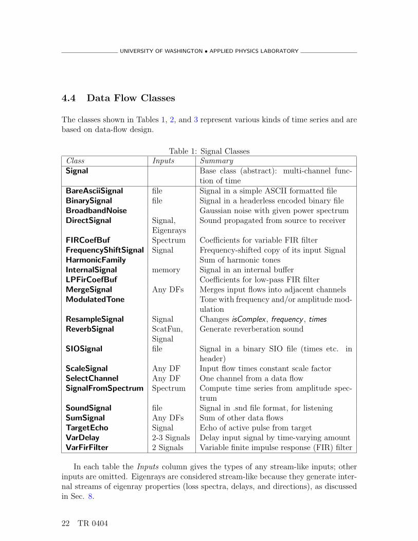
4.4 Data Flow Classes
The classes shown in Tables 1, 2, and 3 represent various kinds of time series and arebased on data-flow design.
Table 1: Signal ClassesClass Inputs SummarySignal Base class (abstract): multi-channel func-
tion of timeBareAsciiSignal file Signal in a simple ASCII formatted fileBinarySignal file Signal in a headerless encoded binary fileBroadbandNoise Gaussian noise with given power spectrumDirectSignal Signal,
EigenraysSound propagated from source to receiver
FIRCoefBuf Spectrum Coefficients for variable FIR filterFrequencyShiftSignal Signal Frequency-shifted copy of its input SignalHarmonicFamily Sum of harmonic tonesInternalSignal memory Signal in an internal bufferLPFirCoefBuf Coefficients for low-pass FIR filterMergeSignal Any DFs Merges input flows into adjacent channelsModulatedTone Tone with frequency and/or amplitude mod-
ulationResampleSignal Signal Changes isComplex , frequency , timesReverbSignal ScatFun,
SignalGenerate reverberation sound
SIOSignal file Signal in a binary SIO file (times etc. inheader)
ScaleSignal Any DF Input flow times constant scale factorSelectChannel Any DF One channel from a data flowSignalFromSpectrum Spectrum Compute time series from amplitude spec-
trumSoundSignal file Signal in .snd file format, for listeningSumSignal Any DFs Sum of other data flowsTargetEcho Signal Echo of active pulse from targetVarDelay 2-3 Signals Delay input signal by time-varying amountVarFirFilter 2 Signals Variable finite impulse response (FIR) filter
In each table the Inputs column gives the types of any stream-like inputs; otherinputs are omitted. Eigenrays are considered stream-like because they generate inter-nal streams of eigenray properties (loss spectra, delays, and directions), as discussedin Sec. 8.
22 TR 0404

UNIVERSITY OF WASHINGTON • APPLIED PHYSICS LABORATORY
Table 2: Spectrum ClassesClass Inputs SummarySpectrum (abstract) Base class: multi-channel function of fre-
quency and timeAsciiSpectrum file Spectrum in an ASCII text fileBinarySpectrum file Spectrum in a plain binary fileDirectSpectrum Spectrum,
EigenraysSpectrum of sound propagated from source toreceiver
FactorSpectrum Spectrum Cholesky factorization (matrix square root)of a power spectrum
GaussianSpectrum Spectrum Generate Gaussian random realization of aspectrum
InternalSpectrum memory Spectrum in an internal bufferReverbSpectrum ScatFun,
SpectrumConvolve reverberation ScatFun with pulsespectrum
SIOSpectrum file Spectrum in a binary SIO file (times, frequen-cies, etc. in header)
SpectrumFromSignal Signal Analyze a Signal into a time-dependent Spec-trum
UnfactorSpectrum Spectrum Square a factored Spectrum to get back apower spectrum
VarSpectFilter Spectrum,Signal
Frequency Domain Finite Impulse Responsefilter
Table 3: Scattering Function ClassesClass Inputs SummaryScatFun (abstract) Base class: multi-channel function of Doppler,
frequency, and timeAsciiScatFun file A ScatFun in a simple ASCII formatted fileBBBDirectionalScat Eigenrays Broadband Bistatic Scattering Function using
spherical tesselationBBBScatFun Eigenrays Compute a Broadband Bistatic Scattering
FunctionInternalScatFun memory A ScatFun in an internal bufferSIOScatFun file A ScatFun in a binary SIO file
TR 0404 23

UNIVERSITY OF WASHINGTON • APPLIED PHYSICS LABORATORY
Classes with “file” or “memory” in the Inputs column are read-write, and the restare read-only. The “file” or “memory” referred to in that column can be used forinput, output, or both. The samples in the “memory” classes can be used as inputby setting the values from the command language as in the example in Sec. 4.3; theycan be used as output by printing the object using SST’s print command; or theycan serve as temporary storage, written by one CopySignal command and read byanother. The “file” classes can be uses similarly, except the samples are in a separatefile.
Classes with “Any DF” or “Any DFs” in the Inputs column can accept as inputsclasses from any of the three data flow hierarchies Signal, Spectrum, or ScatFun.They are “chameleons” that take on the logical character of their inputs. For example,a SumSignal object that has ScatFun objects as its inputs effectively becomes aScatFun, and can be copied into an output ScatFun subclass such as SIOScatFun.The extra attributes that come with ScatFun (e.g. the dopplers grid) tunnel throughthe SumSignal from the inputs to the result. Unfortunately, this masquerade isincomplete: The chameleon classes can be used as inputs to other chameleon classesor the CopySignal command (which has a similar chameleon character), and theycan be used anywhere that a Signal is required, but they cannot be used in othercontexts where a Spectrum or ScatFun is required.
A few of the classes in Tables 1, 2, and 3 are high-level classes that are essentialparts of the user’s view of SST. These include BBBScatFun, DirectSignal, Reverb-Signal, SumSignal, and TargetEcho; each of these classes will be discussed in moredetail in subsequent sections. The rest are storage options, classes used internallyby higher-level classes, and utilities that SST users have found useful. All of themare available for use by SST users through the command language, and all of themcan be substituted anywhere that an object of the base class is required (subject toread/write constraints).
4.5 Basic Signal Operations
Signal processing operations are handled by those classes in Tables 1 and 2 that acceptonly other signals or spectra as inputs. Some of these have already been described,and others are simple and obvious. That leaves a few operations that are central toSST’s operation: delays, filters, and noise generation.
24 TR 0404

UNIVERSITY OF WASHINGTON • APPLIED PHYSICS LABORATORY
4.5.1 Variable Delays
Ideally, SST class VarDelay accomplishes the following:
yc(t) = xc(t− Tc(t)), (13)
where xc(t) is the input signal to be delayed (attribute inSignal). The time-varyingdelay Tc(t) is the sum of two input Signal objects: a single-channel commonDelayBufto be applied to all channels, and a multi-channel channelDelayBuf to be appliedseparately to corresponding channels of the signal. Either of the two delays may beomitted. Typically, the delays vary much more slowly than the signal itself, so thesampling rate for the delays is much lower than that of the input signal (typically afew samples per second or less). For example, in one application Tc(t) is the soundpropagation delay along one ray path from the source to the receiver, which changeswith time because the source and receiver are moving.
The algorithm involves two interpolations. First, the delay Tc(t) is interpolatedto the sample times required for the output signal yc(t). Because Tc(t) varies slowly,this first interpolation is always linear. Second, the input signal xc(t − Tc(t)) isinterpolated to the times given by the output sample times minus the interpolateddelay. Typically this second interpolation must be done using a relatively high order;i.e., one must make use of a relatively large number of samples of the input signal inthe neighborhood of each desired time t− Tc(t).
The ideal band-limited interpolation formula, Eq. (3), has the disadvantage that ithas a very long decay time — all of the samples in the signal are required to computea single interpolated value. The first of two compromises used by class VarDelay isto introduce a window function to limit the number of samples used:
yc(t) =
M/2−1∑k=−M/2
d
(t− tn′
h+ k
)xc(tn′ − kh), (14)
where M−1 is the interpolation order (determined by the order attribute of the inputsignal xc(t)) and tn′ is the largest input sample time less than the desired time:
n′ = b(t− t0)/hc. (15)
The interpolation weights d(z) are the ideal weights from Eq. (3) multiplied by aHann window of length M samples:
d(z) = cos2(πz/M)
(sin(πz)
πz
), (16)
TR 0404 25

UNIVERSITY OF WASHINGTON • APPLIED PHYSICS LABORATORY
where −M/2 ≤ z ≤ M/2. When the order is 3 or less (M ≤ 4), polynomial interpo-lation is used instead of Eq. (16).
The second compromise (if M > 4) is to tabulate the interpolation coefficients toavoid re-calculating them, using a time grid that is L times finer than the grid usedfor the signal:
d(z) ≈ d
(⌊z
L+
1
2
⌋L
). (17)
The sub-sampling ratio L can be specified by the user, but the default value of 512is almost always sufficient.
To determine what interpolation order to use, it is helpful to view the interpolationalgorithm as a band-pass filter. The spectrum of a discrete-time sampled signalconsists of repeated copies of the desired spectrum, one within the Nyquist band(Eq. (2) or (6)) and others above and below the Nyquist band [Oppenheim Schafer1989]. Interpolating it to a band-limited continuous signal is equivalent to filteringout all of the extra copies outside the Nyquist band.
In the ideal version of Eq. (3), the filter has a spectral response of unity throughoutthe Nyquist band, and zero elsewhere. Using a window function to reduce the filterlength makes this transition more gradual. The width of this transition zone, for anM -sample Hann window, is roughly 2.5/(Mh) (from table 7.2 of [Oppenheim Schafer1989]). Our objective is for the filter to have a spectral response near unity overthe part of the Nyquist band in which the signal has significant power. In addition,we want the response to decrease to essentially zero at the locations of those extracopies, outside the Nyquist band, that must be filtered out. In between, near the edgeof the band, a finite-length filter produces an incorrect result — so we must ensurethat there are clear zones near the band edges where the input signal does not havesignificant power.
The suggested rule of thumb: if the significant parts of the signal cover a fractionα of the Nyquist band (in the range F ± α/(2h) for complex signals, or 0 to α/(2h)for real signals), use an interpolation order M − 1 satisfying
M ≥ 2.5/(1− α). (18)
For example, for the common case of 80% band coverage (α = 0.8), at least M = 13is required. Even values of M (odd values of the Signal attribute order) are slightlymore efficient, so order should be 13 or more.
The default value of order is 5, which is appropriate for no more than 50% bandcoverage.
26 TR 0404

UNIVERSITY OF WASHINGTON • APPLIED PHYSICS LABORATORY
4.5.2 Variable Finite Impulse Response Filters
SST needs filters whose spectral response depends (slowly) on time as well as fre-quency:
yc(t) =
∫ ∞
−∞hc(τ, t) xc(t− τ) dτ, (19)
where the filter impulse function hc(τ, t) should ideally satisfy
hc(τ, t) =
∫ ∞
−∞Hc(f, t) e2πifτ df, (20)
where Hc(f, t) is the filter’s specified time-dependent spectral response. This treat-ment differs from the usual textbook case in that both Hc(f, t) and hc(τ, t) dependparametrically on time t. As written, this is theoretically sloppy (what does Hc(f, t)really mean?), but as a practical matter it can be rescued by requiring that thechange in Hc(f, t) is negligible over intervals of t comparable to the range of τ [thewidth of the impulse response hc(τ, t)]. Equivalently, we require that the frequencyresponse Hc(f, t) varies slowly in frequency on a scale given by the inverse of the scaleof its time variation. For example, in one application Hc(f, t) is the sensitivity of abeam pattern to broadband sound arriving along one ray path from the source to thereceiver, which changes with time because the source and receiver are maneuvering.
To eliminate the infinities in the integration limits (making a finite impulse re-sponse, or FIR, filter), we use the window method [Oppenheim Schafer 1989]: Eq. (20)is replaced by
hc(τ, t) = w(τ)
∫ F+1/(2h)
F−1/(2h)
Hc(f, t) e2πifτ df , (21)
where w(τ) is a smooth window function whose length is short compared to the scaleon which Hc(f, t) varies with time t, and whose Fourier transform is narrow on thescale on which Hc(f, t) varies with frequency f .
The choice of w(τ) enforces the smoothness requirements of the previous para-graph. The actual frequency response of this filter is the convolution of the desiredfrequency response, Hc(f, t), with the Fourier transform of the window, W (f). Hence,W (f) should have a narrow central peak and low sidelobes. This issue is discussed atlength in signal processing texts [Oppenheim Schafer 1989]. SST uses a Hann (cosinesquared) window.
SST Class: Class VarFirFilter implements the discrete version of Eq. (19), givenan input signal xc(t) and a stream of filter coefficients hc(τ, t) sampled in both τand t. Normally the sample interval in t for the coefficients is much larger than thesample interval common to τ and the signal. For a given lag τ the coefficients are
TR 0404 27

UNIVERSITY OF WASHINGTON • APPLIED PHYSICS LABORATORY
interpolated linearly in t between the input samples. The convolution is done directly,in the time domain, if the filter is short. For longer filters the convolution is doneusing fast Fourier transforms (FFTs). The break-even point, determined empirically,is currently at 48 samples in τ ; the user can adjust it via a global parameter namedfirFourierCutoff .
SST Class: Class FIRCoefBuf is a data-flow class whose input stream is a time-dependent spectrum Hc(f, t) giving the desired filter response, and whose output isa stream of filter coefficients hc(τ, t). Most of its work is done by class FIRCoef.Together, these classes implement Eq. (21).
SST Class: Class VarSpectFilter is equivalent to VarFirFilter, except that its in-put and output signals are in the windowed frequency domain representation (Eq. (7)).Because FIRCoefBuf uses FFTs whenever it is faster than the time domain implemen-tation, VarSpectFilter is advantageous only if the input is already in the frequencydomain, or if the desired output is in the frequency domain, or if several filters areto be applied consecutively and the filters are relatively long. VarSpectFilter is usedinternally to implement class DirectSpectrum, which is discussed in Sec. 8.
4.6 Generating Signals
Most of SST is about what happens to signals between a source and a receiver. Butwhere do the original signals come from? One option is from “outside”: SST can readsignals, spectra, and scattering functions in all of the same file formats that it usesfor writing them (the entries with “file” or “memory” under the “Inputs” column inTables 1, 2, and 3). If measured data or externally generated signals are available,simply put it in one of those forms to use it as an input to SST. If the external signalisn’t quite right, use SST’s signal processing tools (or external tool collections likeMatlab) to filter, sum, delay, or resample them.
Most SST simulations, however, have no need of external input signals becauseSST provides a useful collection of simple tools to generate signals having specifiedproperties. The remainder of this section outlines those tools.
4.6.1 Generating Gaussian Noise
Gaussian noise with a specified power spectrum can be used as a component of thesignal put into the water by a source like a submarine or ship. To do that, use it as thesignal component of a Source (sec. 7). Such noise can also be used as “background”noise, including sonar self-noise and other distributed noise sources for which SST
28 TR 0404

UNIVERSITY OF WASHINGTON • APPLIED PHYSICS LABORATORY
has no explicit model. To do that, use SumSignal to add it to the output signal fromthe simulation.
Given a power spectral density (PSD) Pcc′(f, tu), our objective is to generate amulti-channel Gaussian random signal xc(t) such that applying Eqs. (7) and (12)returns a close approximation to the original PSD. Such a signal is a “realization” ofthe original PSD. To be more precise, if the expectation operator E {·} in Eq. (12) isreplaced by an average over independent realizations, that average should convergeto the original PSD as the number of realizations increases. This is a well-definedand common problem for stationary, single-channel signals, and extending the usualmethods to multiple channels is straightforward. Stationary, in this context, meansthe PSD Pcc′(f, t) is independent of time t.
To extend it efficiently to a nonstationary PSD, an additional assumption is re-quired: that an update interval ∆ exists such that the time variation of Pcc′(f, tu) isslow on a scale of ∆ and the frequency variation is slow on a scale of 1/∆. Under thoseconditions, the following variant of the method of Mitchell and McPherson [MitchellMcPherson 1981] generates acceptable Gaussian realizations of Pcc′(f, tu).
The first step is to factor the PSD: A generator Gcc′(f, tu) is needed that satisfies
Pcc′(f, tu) =∑c′′
Gcc′′(f, tu) G∗c′c′′(f, tu). (22)
This factorization always exists because, for any given frequency f and time tu, thematrix Pcc′(f, tu) is non-negative definite (its eigenvalues are positive or zero). Thisfactorization is not unique, and there are several good ways to compute Gcc′(f, tu);SST uses Cholesky factorization [Golub Van Loan 1996], which is fast, reasonablystable, and produces a triangular result.
The second step is to multiply the generator by a vector of independent, complex,unit-variance Gaussian random numbers gc(f, tu)
Xc(f, tu) =∑
c′
Gcc′(f, tu) gc′(f, tu), (23)
where the random numbers satisfy
E {gc(f, tu)g∗c′(f ′, tu′)} = δcc′ δuu′ δ(f − f ′), (24)
where δcc′ is a Kronecker delta function and δ(x) is a Dirac delta function. Of course,in the discrete domain the Dirac delta is effectively replaced by the Kronecker delta.
TR 0404 29

UNIVERSITY OF WASHINGTON • APPLIED PHYSICS LABORATORY
The third step is the same as Eq. (9): Inverse Fourier transform, window, andadd. However, for this application the requirement on the post-window function is∑
u
|w′(t− tu)|2 = 1 (25)
instead of Eq. (11). This is satisfied, for example, by a set of cosine windows with 50%overlap. However, the Mitchell-McPherson window function [Mitchell McPherson1981], which also satisfies Eq. (25), has somewhat better spectral properties.
SST Classes: The Mitchell-McPherson method of generating nonstationary Gaus-sian noise is implemented by the sequence of FactorSpectrum (Eq. (22)), Gaus-sianSpectrum (Eq. (23)), and SignalFromSpectrum (Eq. (9)). This same sequenceis used within class ReverbSignal to generate realizations of reverberation. For sta-tionary, single-channel noise, a simpler implementation is provided by class Broad-bandNoise.
4.6.2 Generating Harmonic Tone Families
Harmonic tone families normally represent machinery noise. The usual way to gener-ate the noise emitted by a submarine, ship, or weapon is to use SumSignal to combineseveral HarmonicFamily objects with a BroadbandNoise object. The result is usedas the signal component of a Source object representing the vehicle.
The signal generated by a HarmonicFamily object has the following form:
x(t) =∑
n
An cos(2πnf1t + φn), (26)
where the frequency of each term is an integer multiple of f1. The user specifies f1
(attribute fundamental) and a three-column table giving the harmonic number n, theamplitude in decibels (20 log(An)), and the phase at t = 0 in degrees ((180/π)φn) foreach harmonic.
4.6.3 Generating Modulated Tones
Class ModulatedTone is designed primarily to generate the pulses transmitted bythe transmitter of an active sonar system. A ModulatedTone object, or severalModulatedTone objects combined using a SumSignal, may be used to generatealmost any of the pulses commonly used by active sonar systems.
30 TR 0404

UNIVERSITY OF WASHINGTON • APPLIED PHYSICS LABORATORY
The signal generated by a ModulatedTone has the following form:
x(t) = A e(t) cos(φ(t)) (27)
φ(t) = φ0 +
∫ t
t0
m(τ) dτ
e(t) = envelope(t)
m(τ) = 2π frequencyModulation(τ)
A = 10level/20
φ0 = (π/180) startingPhase
where envelope, frequencyModulation, level , and startingPhase are user-specified at-tributes of class ModulatedTone. In particular, envelope and frequencyModulation,which specify the time-dependent amplitude and frequency of the generated tone, arefunction objects (objects of any subclass of base class Function) that can representany arbitrary function of time. Often objects of class TableFunction are used here.The window functions described in Sec. 4.7 are often useful for the envelope attribute.If envelope is omitted, it is a constant function with value 1.0. If frequencyModulationis omitted for complex envelope signals, it is a constant function whose value is thesignal’s center frequency (F in Eq. (4)).
The integration used to compute the phase φ(t) in Eq. (27) is done numericallyusing two-point (third order) Gaussian integration from each output sample to thenext. This is exact for polynomial frequency modulation functions up to cubic. Thephase is always continuous throughout the pulse sequence.
The SST Web contains examples showing how to use ModulatedTone to specifyshaded pure-tone pulses, FM sweeps, and sequences of shaded or unshaded tones orsweeps. When used with SumSignal, ModulatedTone can also generate chords andother non-sinusoidal signals.
4.7 Window Functions
Table 4 shows the window functions that SST provides for use with Spectrum-FromSignal, SignalFromSpectrum, or ModulatedTone. Those marked “Squared,Eq. (25)” in the “Sum Rule” column are appropriate for generating noise or reverber-ation. Those listing “Linear, Eq. (11)” can be used as either the pre-window w(t) orthe post-window w′(t) for transforming signals between time-domain and windowedfrequency-domain representations (Eqs. (7) and (9)), provided the other window is aRectangularWindow. Window functions used for power spectrum analysis (Eq. (12))or as the envelope of a shaded ModulatedTone need not satisfy any particular sum
TR 0404 31
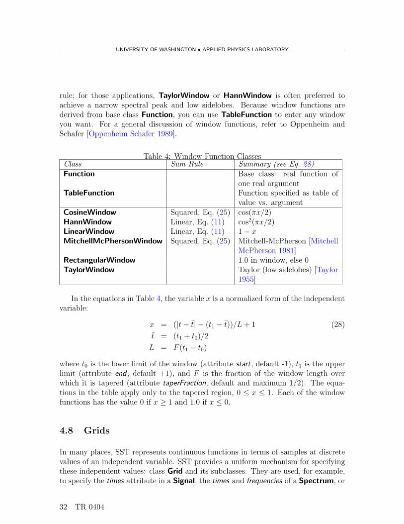
UNIVERSITY OF WASHINGTON • APPLIED PHYSICS LABORATORY
rule; for those applications, TaylorWindow or HannWindow is often preferred toachieve a narrow spectral peak and low sidelobes. Because window functions arederived from base class Function, you can use TableFunction to enter any windowyou want. For a general discussion of window functions, refer to Oppenheim andSchafer [Oppenheim Schafer 1989].
Table 4: Window Function ClassesClass Sum Rule Summary (see Eq. 28)Function Base class: real function of
one real argumentTableFunction Function specified as table of
value vs. argumentCosineWindow Squared, Eq. (25) cos(πx/2)HannWindow Linear, Eq. (11) cos2(πx/2)LinearWindow Linear, Eq. (11) 1− xMitchellMcPhersonWindow Squared, Eq. (25) Mitchell-McPherson [Mitchell
McPherson 1981]RectangularWindow 1.0 in window, else 0TaylorWindow Taylor (low sidelobes) [Taylor
1955]
In the equations in Table 4, the variable x is a normalized form of the independentvariable:
x = (|t− t| − (t1 − t))/L + 1 (28)
t = (t1 + t0)/2
L = F (t1 − t0)
where t0 is the lower limit of the window (attribute start, default -1), t1 is the upperlimit (attribute end , default +1), and F is the fraction of the window length overwhich it is tapered (attribute taperFraction, default and maximum 1/2). The equa-tions in the table apply only to the tapered region, 0 ≤ x ≤ 1. Each of the windowfunctions has the value 0 if x ≥ 1 and 1.0 if x ≤ 0.
4.8 Grids
In many places, SST represents continuous functions in terms of samples at discretevalues of an independent variable. SST provides a uniform mechanism for specifyingthese independent values: class Grid and its subclasses. They are used, for example,to specify the times attribute in a Signal, the times and frequencies of a Spectrum, or
32 TR 0404

UNIVERSITY OF WASHINGTON • APPLIED PHYSICS LABORATORY
the times, frequencies, and dopplers of a ScatFun. They are also used to specify theindependent variables of TableFunction or TableFunction2 objects, which can beused to specify window functions, the power spectrum in BroadbandNoise, and en-vironmental parameters such as sound speed versus depth, volume absorption versusfrequency, or ocean depth versus location.
Class Grid is the base class for a family of classes designed to specify an orderedset of values of an independent variable where some function is to be evaluated,or sampled. UniformGrid is the simplest subclass of Grid, in which the intervalbetween adjacent values is constant (Eq. (1)). Other members of the family includeGeometricGrid (in which the ratio between adjacent values is constant), ListGrid(for arbitrary values), and SubGrid (a subset of values from some other Grid).
5 The Eigenray Model
The model that describes how sound is transformed as it propagates from one partof the ocean to another — the eigenray model — is central to SST’s operation.This transformation requires two time-dependent sets of inputs: the sound to betransformed, and the set of losses and delays to be applied to that sound. Theeigenray model supplies the second set in the form of a finite list of eigenrays, eachof which represents a distinct path by which sound can travel from one place in theocean to another. Each eigenray takes as its input the source and receiver locations inthe ocean, rS and rR. Given that pair, eigenray p produces the following information:
• Tp(rR, rS) is the propagation delay for path p; i.e., the time required for soundto travel from one end of the path to the other.
• Lp(f, rR, rS) is the complex-valued propagation loss factor for path p includingspreading loss, boundary reflection loss, and volume absorption. Its unit isinverse length (m−1). It gives the ratio of the sound pressure at rR to thetransmitted sound pressure at rS reduced to a distance of one meter, as afunction of acoustic frequency f .
• SSp(rR, rS) = ∇STp(rR, rS) is the slowness vector at the source, which is de-fined as the spatial gradient of the time delay with respect to the source locationrS. Its direction is opposite the direction of propagation along the eigenray atthe source, and its magnitude is the inverse of the local sound speed at thesource.
TR 0404 33

UNIVERSITY OF WASHINGTON • APPLIED PHYSICS LABORATORY
• SRp(rR, rS) = ∇RTp(rR, rS) is the slowness vector at the receiver R; i.e., thespatial gradient of the time delay with respect to the receiver location rR. Itpoints in the direction of propagation along the eigenray at the receiver, andits magnitude is the inverse of the local sound speed at the receiver.
At one level, the eigenray model consists of a finite set of maps whose inputs are twoend-point locations, rR and rS, and whose outputs are the four pieces of informationlisted above: Tp, Lp(f), SSp, and SRp.
At a slightly higher level, the presence of the gradients SSp and SRp suggests useof a first-order Taylor expansion to compute the time delay, not just between thegiven end points, but between two points in small neighborhoods around the givenend points:
Tp(rR + ρR, rS + ρS) = Tp(rR, rS) + SRp · ρR + SSp · ρS + · · · , (29)
where the offset vectors ρR and ρS are assumed to be small compared to the totalpropagation distance. This is useful because sources and receivers have finite size.Given an eigenray from one point on the source to one point on the receiver, thisexpansion can be used to compute (approximately) the delay from any part of thesource to any part of the receiver.
For most purposes the “local plane wave” approximation (first-order Taylor ex-pansion) of Eq. (29) is sufficient. However, for a long array and a source at shortrange, wave-front curvature may be significant. More to the point, large-aperturepassive sonars like towed arrays use wave-front curvature as an important clue forestimating target range. The eigenray model does not give enough information for afull second-order expansion of the time delay, but SST gets part way there using aspherical wave approximation. In this approximation, the wave front at each end islocally spherical, with a center located at the apparent location of the other end asinferred from the time delay and the local sound speed. Each of the dot products inEq. (29) is replaced by a second-order expression of the form
τp(S, ρ) = S · ρ +|S|2|ρ|2 − (S · ρ)2
2Tp
. (30)
This approximation is good for straight-line propagation, and remains useful for hor-izontal curvature in most scenarios. It is less trustworthy for vertical curvature in thepresence of ray bending.
Another important property is that the delay Tp does not depend on frequencybecause the ocean is nondispersive; i.e., the dependence of the sound speed on fre-quency is very weak [Urick 1983]. Small violations of the nondispersive assumptioncan be absorbed into the phase of the complex loss Lp(f, rR, rS).
34 TR 0404

UNIVERSITY OF WASHINGTON • APPLIED PHYSICS LABORATORY
It is equally important to note that the eigenray model does not give gradientsof the propagation loss Lp(f, rR, rS). This is a value judgment, not a fundamentallimitation. The eigenray model computes the gradients of time delay because beamformers are very sensitive to variation in propagation time between one part of asource or sonar and another part. However, variation in propagation loss in a regionthe size of a source or sonar is not so important, so it is ignored. The loss Lp(f, rR +ρR, rS + ρS) is assumed to be independent of ρR and ρS over such regions. Largesonar arrays or targets for which these assumptions do not hold can still be modeled,but to do so SST must treat them as compact groups of elements or highlights, andexplicitly compute the eigenrays to the center of each group.
Thus, at the second level, the inputs to the eigenray model are not two points,but two regions around those points. For each eigenray, the eigenray model gives theloss and delay from any point in one region to any point in the other region.
There is a third level, too: the eigenray model specifies a linear transformationwhose input is a sound source field qS(t, r) emitted from various parts of a sourcein the neighborhood of rS, and whose output is the resulting sound field p(t, r) inthe neighborhood of rR. SST assumes that this transformation has the followingmathematical form (in the time domain):
pR(t, rR + ρR) =∑
p
∫ ∫lp(τ, rR, rS) (31)
×qS (t− Tp(rR + ρR, rS + ρS)− τ, rS + ρS) dτ dρS.
The offset vectors ρR and ρS have the same scale as the size of the receiver andsource, respectively, and are assumed to be small compared to the total propagationdistance. The sum is over eigenrays (paths) p.
The propagation impulse response lp(τ, rR, rS) in Eq. (31) is the inverse Fouriertransform of the propagation loss:
lp(τ, rR, rS) =
∫ ∞
−∞Lp(f, rR, rS) e2πifτ df. (32)
Because Lp(f, rR, rS) varies slowly with frequency, lp(τ, rR, rS) is sharply peaked intime delay τ . Eq. (31) will be combined with the source and receiver models in Sec. 8.
5.1 Straight-line Eigenray Model
Of SST’s three choices for the eigenray model, the only one that is contained entirelywithin the SST software is the base class, EigenrayModel. This model is valid only
TR 0404 35

UNIVERSITY OF WASHINGTON • APPLIED PHYSICS LABORATORY
if the sound speed is independent of depth and location, the ocean depth is constant,and the surface and bottom properties are the same everywhere. Sound travels instraight lines except where it reflects in the specular (mirror) direction from thesurface or bottom.
SST computes the eigenrays using the method of images. Effectively, the soundtravels in a straight line from the source to an image of the receiver, which is placed atthe apparent location of the receiver as seen from the source, possibly via surface andbottom reflections. Each image is above or below the actual position of the receiver,by a distance that depends on the ocean depth and the number and order of thereflections. The vector from the source to the image of the receiver for path p is givenby
Rp = rR − rS − 2|Sp −Bp|zRz ± 2BpDz (33)
where Bp is the number of bottom reflections for path p, Sp is the number of surfacereflections, D is the ocean depth, rR is the receiver location, rS is the source location,z is a unit vector in the z direction (down), and zR = rR · z is the receiver depth. Thesign of the last term is + if the reflection closest to the source is from the bottom, or− if it is from the surface. There are four images (i.e., four paths p) for each nonzerovalue of Bp: Sp = Bp − 1, Sp = Bp + 1, and two with Sp = Bp.
The time delay for path p is
Tp = Rp/c (34)
where Rp = |Rp| is the slant range from the source to the image of the receiver andc is the sound speed.
The propagation loss includes spherical spreading, volume absorption, and reflec-tion losses:
Lp(f) = R−1p eα(f)Rp [LS(s, f)]Sp [LB(s, f)]Bp (35)
where LS(s, f) is the reflection loss for each surface bounce, LB(s, f) is the reflectionloss for each bottom bounce, s is the sine of the grazing angle, f is the frequency,and α(f) ≤ 0 is the volume absorption rate per meter (from the volume attenuationmodel, Sec. 6.3).
The slowness vectors are given by:
SRp = Rp/(cRp) (36)
SSp = −Rp/(cRp)
except that the sign of the vertical (Z) component of SRp is reversed if the totalnumber of bounces, Sp + Bp, is odd.
36 TR 0404

UNIVERSITY OF WASHINGTON • APPLIED PHYSICS LABORATORY
5.2 CASS/GRAB Eigenrays
The Comprehensive Acoustic System Simulation (CASS) [Weinberg et al. 2001] soft-ware, developed by Henry Weinberg and others at NUWC Newport, models oceans inwhich the sound speed may vary with all three dimensions, and the bathymetry andbottom type may depend on horizontal location. The eigenrays can bend, and thedirection of the forward bottom reflection depends on the local bottom slope. CASSis a self-contained modeling environment that can compute and plot many differentresults of interest for sonar analysis and performance prediction. The only componentof CASS used by SST is the Gaussian Ray Bundle (GRAB) [Weinberg Keenan 1996]eigenray model.
CASS produces eigenrays in external files, which SST reads and uses in its simula-tions. Two different SST classes may be used, depending on the relationship betweenthe CASS run and the SST run. The recommended choice is to run only SST, andspecify class CASSEigenrayRun for the eigenray model. In that case, SST generatesthe CASS input files based on its own input parameters, and runs CASS as a sub-process. This is the recommended choice in most cases because SST ensures that theCASS and SST run streams are consistent. It is also less work than CASSEigenray-Model because you need to prepare only SST’s input files, not CASS’s.
SST users may choose to prepare CASS input files, run CASS to generate eigen-rays, and then run SST independently. In that case, choose class CASSEigenray-Model and specify the names of the eigenray files that CASS wrote. This is stronglydiscouraged because it is very difficult to maintain consistency between CASS andSST. CASSEigenrayModel remains in SST primarily to facilitate testing.
5.3 Generic Sonar Model (GSM) Eigenrays
The Generic Sonar Model (GSM) [Weinberg 1985], a much older product of HenryWeinberg at NUWC, models oceans in which the sound speed may depend only ondepth. The sound speed, ocean depth, and boundary properties are assumed to beindependent of horizontal location (range independent). GSM includes five differentuser-selectable eigenray models, of which the most useful with SST (in our opinion)are the Multipath Expansion (MULTIP) and Fast Multipath Expansion (FAME)models.
Use of GSM is somewhat simpler than use of CASS, but otherwise very similar.Like CASS, GSM can be run separately before SST, using the SST class GSMEigen-rayModel. Your other choice is to run only SST, specifying class GSMEigenrayRun
TR 0404 37
UNIVERSITY OF WASHINGTON • APPLIED PHYSICS LABORATORY
for the eigenray model; SST then runs GSM as a subprocess. The same issues ofconsistency arise with GSM as with CASS, but because GSM is simpler, the prob-ability of getting it right with GSMEigenrayModel is somewhat better than withCASSEigenrayModel. Nevertheless, GSMEigenrayRun is the recommended option.
NUWC no longer supports GSM. We continue to support its use in SST, at leastuntil our users have time to convert their SST scripts to CASS.
5.4 Eigenray Interpolation and Ray Identity
For many reasons, it is important that the delay, loss, and slowness vectors for agiven eigenray are continuous functions of the end points rR and rS. Continuityof the delay Tp is especially important, in part because the first derivative of thedelay is the Doppler shift, to which many sonar receivers are especially sensitive.Achieving continuity for the straight-line eigenray model is easy because its propertiesare computed as needed, and because the identity of each eigenray is uniquely specifiedby the number and order of its surface and bottom reflections.
For both CASS and GSM eigenrays, the eigenray files read by SST contain eigen-rays (sets of eigenray properties) at discrete values of the end point locations. Valuesbetween those locations must be computed using interpolation. Given a list of eigen-rays at one location and another such list at a neighboring location, we are faced withthe problem of matching the members of one list with the members of the other listin such a way that it makes physical sense to interpolate eigenray properties betweenthe matching eigenrays at different locations. Matching eigenrays are assigned to asingle ray (an object of some subclass of base class Ray). The expectation is that fora given ray object identified by index p, the maps from the location pair (rR, rS) tothe properties Tp, Lp(f), SSp, and SRp are continuous and physically meaningful.
CASS and GSM help with this matching by providing a signature for each eigenray,consisting of the numbers of surface bounces, bottom bounces, upper vertexes, andlower vertexes for each one. Unfortunately, the signature is not sufficient to specifyuniquely how to match eigenrays at different locations because there can be anynumber of eigenrays (including zero) with the same signature for the same locationpair, and that number can change from location to location.
At the start of a simulation, SST reads the CASS or GSM eigenray files into itsmemory and organizes them into a set of internal tables designed to support interpo-lation in the tables. To do this, each set of eigenray properties read from the files isassigned a ray identity, and eigenrays with the same identity are eventually mappedinto the same ray object. Eigenrays with the same signature are assigned their ray
38 TR 0404
UNIVERSITY OF WASHINGTON • APPLIED PHYSICS LABORATORY
identities using a complex set of heuristics that take into account the closeness of theattributes (especially delay) of one eigenray to a simple extrapolation of the attributesof an adjacent eigenray. These heuristics work well in our tests, but our tasks wouldbe much easier and our confidence would be higher if the eigenray models provided aunique signature to support unambiguous matching for interpolation.
6 Ocean Model
The primary inputs to the eigenray model (besides the locations of the end points)come from properties of the ocean, which is an object of class Ocean. The propertiesused as inputs to the eigenray model are the depth, sound speed, volume attenua-tion, and the reflection coefficients of the surface and bottom. These properties areused directly by the straight-line EigenrayModel, and they are passed in table formto CASS or GSM by class CASSEigenrayRun or GSMEigenrayRun, respectively.Classes CASSEigenrayModel or GSMEigenrayModel do not use them, since theyget their inputs from the user-supplied CASS input file.
In addition, class Ocean supplies the scattering strengths used by SST’s rever-beration model, which will be described in Sec. 10.
6.1 Ocean Depth
The depth attribute of class Ocean is, in general, a function of horizontal locationD(x, y), in meters, with x and y in meters north and east of an arbitrary origin. Itstype is class Function2, which is an abstract base class for describing any real-valuedfunction of two real variables. That means the user can assign to depth an object ofany subclass of Function2. By default, it is an object of class ConstantFunction2;the user simply assigns a value, e.g., “ocean.depth = 200”.
If CASS eigenrays are used, the bathymetry can be specified by assigning to thedepth attribute an object of class TableFunction2, which provides several ways toenter a table of depth on a rectangular grid versus horizontal location (meters northand east of an arbitrary origin). Interpolation in the table is normally bilinear (order1), although the user can specify the order up to cubic (order 3).
Alternatively, assign to Ocean’s depthFile attribute the name of a file in CASS’sinput format containing a “BOTTOM DEPTH TABLE” section. SST will search for thatsection, parse it, extract the bathymetry, and build a TableFunction2 object fromthe data.
TR 0404 39

UNIVERSITY OF WASHINGTON • APPLIED PHYSICS LABORATORY
6.2 Ocean Sound Speed
The soundspeed attribute of class Ocean is, in general, a function of depth c(z) inmeters per second, versus depth z in meters. Its type is class Function, which is anabstract base class for describing any real-valued function of one real variables. Bydefault, it is an object of class ConstantFunction; the user simply assigns a value,e.g., “ocean.soundspeed = 1500”. The default value is 1520 m/s.
If CASS or GSM eigenrays are to be used, the sound speed profile can be specifiedby assigning to the soundspeed attribute an object of class TableFunction, whichprovides several different ways to enter a table of sound speed versus depth. Thistable is passed to CASS or GSM, which does its own interpolation.
CASS permits the sound speed to depend on horizontal location as well as depth.However, SST does not yet provide a way to specify this horizontal variability.
6.3 Ocean Volume Attenuation
The volumeAttenuation attribute of class Ocean is, in general, a function of frequencyA(f) in dB per km, versus frequency f in Hz. By default, it is an object of classConstantFunction; the user simply assigns a value, e.g., “ocean.volumeAttenuation= -2.1”. The default value is 0 dB/km.
To specify frequency-dependent attenuation, one option is to assign to the vol-umeAttenuation attribute an object of class TableFunction, which allows the user toenter a table of attenuation versus frequency using tables of the same formats usedfor the sound speed. Another option is to assign ThorpAttenuation to the attribute.This option computes the absorption using the expression in [Urick 1983] page 108.
6.4 Surface and Bottom Models
Class Ocean contains attributes surface and bottom, both of which are objects ofclass Boundary. SST users can assign to them any object of any class derived fromBoundary, including APLBottom, JacksonBottom, APLSurface, GilbertSurface,and McDanielSurface.
40 TR 0404

UNIVERSITY OF WASHINGTON • APPLIED PHYSICS LABORATORY
6.4.1 Reflection Coefficients
Each of these classes defines two complex-valued member functions TotalForwardAmpand CoherentForwardAmp, each of which is a function of two arguments, sinAngle(the sine of the grazing angle) and frequency (in Hz).
The straight-line EigenrayModel class uses these functions to compute the factorsLS(s, f) and LB(s, f) in the eigenray propagation loss, Eq. (35); classes CASSEigen-rayRun and GSMEigenrayRun use them similarly. For each boundary, SST calls themember function CoherentForwardAmp when the eigenrays are being used for one-way propagation or target echoes, but it calls TotalForwardAmp when the eigenraysare being used for reverberation. The theory behind this practice is based on thefollowing distinction:
• For reverberation, the distinction between near-specular forward scattering andspecular reflection is unimportant; all that matters is how much energy isremoved from the total. Hence, SST calls TotalForwardAmp, which treatsforward-scattered energy as if it were specularly reflected.
• For passive reception or target echoes, scattered energy is effectively lost be-cause scattering reduces the coherence of the signal (reducing processing gain),stretches it out in time, and spreads it in angle, all of which tend to push itdown under the background. Hence, SST calls CoherentForwardAmp, whichtreats forward-scattered energy as if it were absorbed.
This theory is flawed; for many purposes TotalForwardAmp is too large and Coher-entForwardAmp is too small. We are currently addressing this issue by developingnew algorithms to control the coherence of the simulated signal; the “coherent ver-sus incoherent” dichotomy will be replaced by explicit and quantitative control ofcoherence.
For most purposes the distinction is unimportant anyway because CoherentFor-wardAmp is used only by the straight-line EigenrayModel. If CASSEigenrayRunor GSMEigenrayRun is selected, the TotalForwardAmp function is called repeatedlywith different values of frequency and grazing angle to build a “SURFACE REFLECTION
COEFFICIENT TABLE” and a “BOTTOM REFLECTION COEFFICIENT TABLE” to be passedto CASS or GSM. This tends to overestimate the reflection coefficient, except for re-verberation. The table is passed in decibels; CASS and GSM ignore the phase.
(Note: CASS accepts a table of phase shifts too, but CASSEigenrayRun doesn’tprovide it. This needs to be fixed soon.)
TR 0404 41

UNIVERSITY OF WASHINGTON • APPLIED PHYSICS LABORATORY
6.4.2 Bistatic Scattering Strength
Each Boundary subclass also provides a function called BistaticStrength, denotedSl(f, Sp, Sq). It computes the scattering differential cross section per unit area of theboundary; it is dimensionless (an area divided by an area). It takes as its input afrequency f and two slowness vectors, Sq giving the direction from which incidentsound arrives at the boundary, and Sp giving the direction toward which it scatters.The subscript l denotes a scattering layer (surface or bottom) and the subscripts pand q denote the outgoing and incoming eigenrays.
Most of the Boundary subclasses are fully bistatic. That means the two slownessvectors reduce to at least three independent parameters: two grazing angles (fromthe boundary plane to each of the two slowness vectors) and a bistatic angle (from avertical plane containing one vector to the other vector). Under most conditions, thebistatic strength is strongly peaked in the region of the specular direction.
The older Boundary subclasses, APLBottom and APLSurface, are monostatic.That means they define a backscattering strength Sl(f, sin(θ)), which is a function ofonly one angle, the grazing angle θ. For those classes, the BistaticStrength methodcomputes the backscattering strength for each of the two grazing angles (incoming andoutgoing) and returns the geometric average (the square root of the product). This isthe same form used by CASS. It is a reasonably good approximation for geometriesthat are close to backscattering (i.e., if the two slowness vectors are nearly equal)and for bubble-dominated surface scattering. It is a particularly bad approximationfor the region near the specular direction because it does not produce a peak in thatregion. The monostatic models may be removed in a future SST release.
6.4.3 Boundary Classes
The Boundary classes are listed in Table 5 with the literature references from whichthey were taken and a brief indication of applicability. In the table “high frequency”means over 10 kHz and “mid frequency” means 1 to 10 kHz (roughly).
The base class Boundary allows the user to enter either or both of the reflectioncoefficient functions and the monostatic backscattering strength as tables versus an-gle and frequency. By default the reflection coefficients are unity (no loss) and thebackscattering strength is zero in energy terms (no scattering). Boundary may beused for either the surface or the bottom.
For the surface models APLSurface, GilbertSurface, and McDanielSurface, To-talForwardAmp includes all of the incident intensity except the fraction that is ab-
42 TR 0404

UNIVERSITY OF WASHINGTON • APPLIED PHYSICS LABORATORY
Table 5: Surface and Bottom ModelsClass References UseBoundary Monostatic, table drivenAPLBottom [APL Models 1994, Mourad
Jackson 1989]Bottom, monostatic, highfrequency
JacksonBottom [Williams Jackson 1998, APLModels 1994, Mourad Jackson1993, Mourad Dahl Jackson1991,Moe Jackson 1994, Schul-ten Anderson Gordon 1979]
Bottom, bistatic, mid tohigh frequency
APLSurface [APL Models 1994] Surface, monostatic, highfrequency
GilbertSurface [Gilbert 1993,Kulbago 1994] Surface, bistatic, low to midfrequency
McDanielSurface [McDaniel 1990, Lang Culver1992, Donelan Hamilton Hui1985]
Surface, bistatic, high fre-quency
sorbed by bubbles and converted to heat. CoherentForwardAmp also removes scat-tered intensity using a simple model of surface roughness [APL Models 1994]; thisloss can be very substantial whenever the wave height is comparable to or greaterthan the acoustic wavelength. The only environmental input to these models is thewind speed.
For the bottom models APLBottom and JacksonBottom, the TotalForwardAmpand CoherentForwardAmp are identical. The reflected intensity includes all of theincident intensity except the fraction that is refracted into the bottom, as estimatedusing a lossy Rayleigh coefficient [Mackenzie 1959]. Bottoms of these classes maybe specified using sets of parameters describing surface roughness, sediment soundspeed, absorption rate, and scattering within the sediment. Sets of named bottomtypes (e.g., MediumSand or CoarseSilt) are also provided.
6.5 Volume Scattering Strength
Volume scattering tends to occur in layers because sea life tends to congregate at re-stricted ranges of depth. Therefore, volume scattering is specified in SST by defininga list of ReverbLayer objects, each of which specifies the volume scattering strength(assumed constant) between specified upper and lower depth limits. Currents arespecified by giving the average horizontal velocity of the scatterers in each layer.
TR 0404 43

UNIVERSITY OF WASHINGTON • APPLIED PHYSICS LABORATORY
Currently, SST’s reverberation model (Sec. 10) treats each layer as if all of the scat-terers were concentrated in a thin sheet in the center of the layer.
7 Sonar and Source Models
The sonar model (the box labeled “Sonar Receiver” in Fig. 1) describes any compactobject that can receive sound from the ocean. The source model (the boxes labeled“Sonar Transmitter” and “Source”) describes any compact object that emits soundinto the ocean. These are represented in SST by objects of classes Sonar and Source,respectively. For passive sonar scenarios the Source is whatever the sonar is listeningto. For active sonar scenarios the Source is the transmitter. Other Source objectsmay represent countermeasures, the sonar’s own vehicle, interfering ships in the area,pile drivers, explosions, or anything else that produces sound from a small region.Sonar and Source objects are also used internally to model target echoes (Sec. 9).
Classes Sonar and Source are almost identical. Each object of either of thoseclasses contains the following attributes:
• trajectory : an object of a class derived from base class Traject. It determinesthe location and orientation of the sonar or source platform as a function oftime.
• beams: a list of objects derived from base class Beam. They determine thespatial properties of each channel, including its directional sensitivity and thelocation of its phase center.
• signal : an object of a class derived from base class Signal. For a Source, thisis an input representing transmitted sound. For a Sonar, it is an output repre-senting received sound. (The association of a Signal with a Sonar is implicit;it is not formally an attribute of class Sonar.)
An active sonar system consists of a Sonar and at least one Source. It is mono-static if those components share a single trajectory, and it is bistatic if they havedifferent trajectories.
44 TR 0404

UNIVERSITY OF WASHINGTON • APPLIED PHYSICS LABORATORY
7.1 Trajectories and Coordinate Transformations
In Sonar, Source, and Target objects, the local geometric properties (the locationsand beam patterns of the transducers, sources, or highlights) are expressed in aplatform-centered coordinate system whose components are in the directions (For-ward, Starboard, Below) relative to some arbitrarily defined “center” of a particularplatform (its origin). Global properties of the ocean are expressed in the Earth-centered coordinate system, whose components are in the directions (North, East,Down) relative to an origin at an arbitrary point on the surface of the ocean. Thetime-dependent mapping between the local and global coordinate systems is definedby the trajectory attribute of each vehicle. An SST user specifies the trajectory byassigning to this attribute an object of any subclass of class Traject — usually aTrajectory, but sometimes a CombinedTraject.
Two kinds of vectors need to be transformed between local and coordinate systems:locations and directions (slowness vectors). These transformations take the followinglinear form:
r′ = MX(t) (r − rX(t)) (37)
S′ = MX(t) S ,
where the primed vectors are expressed in platform coordinates and the unprimedvectors are in Earth-centered coordinates. The vector rX(t) is the location of theorigin of platform X, and MX(t) is the 3-by-3 rotation matrix determined by theorientation of the platform (sonar, source, or target). Each vehicle’s trajectory sup-plies the time-dependent location rX(t) and rotation matrix MX(t) used in thesecoordinate transformations.
A Trajectory (the most commonly used subclass of Traject) specifies a body’smotion using a list of Snapshot objects. Each Snapshot is a “picture” of the position,velocity, orientation, and rotation rate of a body (four attributes, three numbers each)at a single specified time. For intermediate times the trajectory is computed usingself-consistent cubic interpolation, in which all four attributes are continuous in time.For times outside the range of the list, each Trajectory is extrapolated using theassumption that the velocity and the rotation rate remain constant in the body’sown coordinate system. Thus, a Trajectory containing a single Snapshot can beused to specify motion in a straight line, a circle, or a helix.
The other Traject subclass is CombinedTraject, which is specified in terms oftwo other Traject objects: one to specify the motion of a body with respect to anintermediate coordinate system, and another to specify the motion of that intermedi-ate coordinate system with respect to a global system. A CombinedTraject can be
TR 0404 45

UNIVERSITY OF WASHINGTON • APPLIED PHYSICS LABORATORY
used anywhere that a Traject is required, but its primary application is internal, inthe implementation of SST’s target models.
Internally, orientations and rotations are represented using quaternions [Dean1966], also known as Cayley-Klein parameters [Goldstein 1950]. This representationis chosen for its combination of compactness with efficient support of coordinatetransformations, composition of rotations, interpolation, and extrapolation.
7.2 Beam Patterns
Each Sonar and each Source contains an attribute called beams, which consists of auser-specified list of objects belonging to classes derived from the base class Beam,one object per channel in the associated signal . Each Beam object provides memberfunctions that compute the following quantities:
• Bc(f, S′): the directional sensitivity pattern used in Eq. (39) (or the corre-sponding one for source beams), given the frequency f and the slowness vectorS′ in platform coordinates. For element-level simulations, this is the sensitiv-ity pattern of one element, as modified by the physical supports and bafflessurrounding it and by any preamplifiers or filters between the element and theinjection point chosen for the simulation. For beam-level simulations, this is theeffective sensitivity pattern of the array plus surrounding hardware, as modifiedby any signal processing steps from the array through the beamformer.
• r′c: the channel offset. This is the location, in platform coordinates, of thephase center of channel c. For element-level simulations, this is the locationof a transducer relative to the array center. For beam-level simulations, it isoften zero, or sometimes the center of a sub-array used to form an “offset phasecenter” beam.
• τp(S′, r′c): the offset delay used in Eq. (31). The expression used is essentially
Eq. (30), using the channel offset r′c in place of ρR and with inputs in platformcoordinates.
Subscript c stands for the receiver channel r or the source channel s.
The various subclasses of class Beam differ from one another in the algorithmused to compute Bc(f, S′). They are listed in Table 6.
The first section in the table contains simple, self-contained beam patterns, mostof which are based on equations in Chapter 3 of [Urick 1983]. For example, Stick-Beam, PistonBeam, and LineBeam come from the first three rows of Urick’s Table
46 TR 0404

UNIVERSITY OF WASHINGTON • APPLIED PHYSICS LABORATORY
Table 6: Beam Pattern ModelsClass SummaryBeam Abstract base classOmniBeam Omnidirectional (1.0 everywhere)BinomialBeam Binomial weighted, steered line arrayConeBeam 1.0 inside a cone, 0 outsideDCLineBeam Dolph-Chebyshev weighted line array [Albers 1965]ElementSumBeam Sum of weighted elements beam patternLineBeam Uniformly weighted, steered line arrayPistonBeam Circular piston transducerRecPistonBeam Rectangular piston transducerStickBeam Continuous, uniform line transducerEBFTableBeam Interpolated from table vs. elevation, bearing, frequencyEFIntensityBeam Intensity vs. sin(elevation) and frequencySIOBeam Table vs. elev, bear, freq in binary SIO fileDecibelBeam Beam pattern transformed from decibels to pressure ratioProductBeam Product of input beam patternsRotatedBeam Beam pattern rotated with respect to the platform coor-
dinatesSumBeam Sum of element beam patternsWeightedBeam Beam pattern multiplied by a weight and phase-shifted for
delay
3.2 (second column, omitting the squaring operation). Each beam pattern object isconstructed using input parameters that differ from class to class. For example, Pis-tonBeam requires a piston diameter and axis direction, whereas LineBeam requiresthe number and spacing of the elements, axis direction, and steering delay.
The classes in the second section in the table accept tables of numbers; Bc(f, S′)is computed by interpolation. EFIntensityBeam and SIOBeam optionally acceptanother beam pattern as input, in which case the table is computed by sampling theinput pattern; the result may be used in this or subsequent runs to speed up thesimulation.
The classes in the third section of the table are transformations that accept oneor more input beam patterns and transform them in some way.
All beam patterns accept, in addition to their class-specific input parameters, anoffset vector r′c and an additional delay to be added to the offset delay τp(S
′, r′c).
TR 0404 47

UNIVERSITY OF WASHINGTON • APPLIED PHYSICS LABORATORY
7.3 Sonar Transformation
The sonar model has a more abstract interpretation: it represents a transformationwhose output is the signal yr(t) in all channels r of receiver R, and whose input isthe sound field in the water, pR(t, r), for r in the neighborhood of the sonar originrR. Such a sound field is produced as the output of the eigenray transformation(Eq. (31)). The sonar transformation takes the following form (in the time domainand platform coordinates):
yr(t) =
∫ ∫br(τ,ρ
′r) p′R(t− τ, r′r + ρ′
r) dτ dρ′r , (38)
where r′r is the channel offset vector provided by the beam pattern model for receiverchannel r (Sec. 7.2). The time-space domain kernel br(τ,ρ
′r) for receiver channel r is
related to the receiver’s beam pattern Br(f, S′) by a four-dimensional spatiotemporalFourier transform:
br(τ,ρ′r) =
∫ ∫Br(f, ν ′/f) e2πi(fτ+ν′·ρ′
r) df dν ′ , (39)
where ν ′ is the wave number vector in vehicle coordinates. The spatial kernel br(τ,ρ′r)
is nonzero over the region ρ′r where the receiver is sensitive. For an ideal piston beam
the sensitive region is the disk at the face of the transducer, although in practiceeffects like baffling and shadowing tend to make it more complicated. SST startsfrom the frequency-direction form, Br(f, S′), where S′ = ν ′/f (beam patterns versusfrequency and look direction).
The primed coordinates in Eqs. (38) and (39) are expressed in a platform-centeredcoordinate system whose origin is at rR(t). Equation (37) defines their relationshipto the unprimed, Earth-centered coordinates used in the eigenray transformation(Eq. (31)).
7.4 Source Transformation
The source model has a similarly abstract interpretation: it represents a transforma-tion whose input is the signal xs(t) emitted through each channel s of the source S,and whose output is the sound source field qS(t, rS + ρS) in the neighborhood of rS.This sound source field is the input of the eigenray transformation (Eq. (31)). Thesource transformation takes the following form (in the time domain):
qS(t, rS + ρS) =∑
s
∫b′s(τ,MS(t) ρS − r′s) xs(t− τ) dτ , (40)
48 TR 0404
UNIVERSITY OF WASHINGTON • APPLIED PHYSICS LABORATORY
where r′s is the channel offset vector provided by the beam pattern model for sourcechannel s (Sec. 7.2). The time-space domain kernel b′s(τ,ρ
′s) for source channel s is
related to the source’s beam pattern Bs(f, S′) as per the receiver (Eq. (39)) exceptfor the sign in the relationship S′ = −ν ′/f . The relations between platform-centered(primed) and Earth-centered (unprimed) coordinates are given by Eq. (37).
8 Direct Sound Propagation Models
The “direct” sound propagation model is a transformation whose input is the soundxs(t) emitted by all channels s of a given source, and whose output is that portionof the received sound yr(t) that does not scatter from objects or irregularities on itsway to receiver channel r. Conceptually, it consists of the successive application ofthe source model, the eigenray model, and the receiver model, whose time-domainexpressions are given by Eqs. (40), (31), and (38), respectively. If we combine thoseequations in series, the spatial integrations reduce to Dirac delta functions and dropout. The remaining operations can be arranged into successive signal transformations,as follows:
xsp(t) = xs (t− Tp − τp(MSSSp, r′s)) (41)
xp(t) =∑
s
∫ [∫e2πifSτ ′
S Bs(fS, MSSSp)dfS
]xsp(t− τ ′S) dτ ′S (42)
yp(t) =
∫ [∫e2πifτ Lp(f)df
]xp(t− τ) dτ (43)
xrp(t) =
∫ [∫e2πifRτ ′
R Br(fR, MRSRp)dfR
]yp(t− τ ′R) dτ ′R (44)
yrp(t) = xrp (t− τp(MRSRp, r′r)) (45)
yr(t) =∑
p
yrp(t). (46)
Thus, the transformation of a source channel signal xs(t) to a receiver channel signalyr(t) involves three filters [source beam pattern Bs(f, S′
Sp), eigenray loss Lp(f), andreceiver beam pattern Br(f, S′
Rp)] plus three delays [source channel offset τp(S′Sp, r
′s),
eigenray Tp, and receiver channel offset τp(S′Rp, r
′r)], plus sums over eigenrays and
source channels. The offset delays are given by Eq. (30). The three inverse Fouriertransforms (in square brackets) compute the time-domain impulse responses for thefilters, and the three time integrations convolve those impulse responses with thesignal.
TR 0404 49
UNIVERSITY OF WASHINGTON • APPLIED PHYSICS LABORATORY
Note that all of the filters and delays depend parametrically on time t because thetrajectory attributes rR, rS, MR, and MS depend on time (the sonar and source canmove), and the eigenray attributes SSp, Tp, Lp(f), and SRp depend on the eigenray’send points rR and rS.
8.1 DirectSignal
Equations (41) through (45) represent “ideal” filters and delays. Their implementa-tion by SST class DirectSignal looks very much like those equations, except that theconvolutions and interpolations are forced to have finite length. For each path p, Di-rectSignal sets up a chain of five “data flow” objects (Sec. 4.3) in series: two VarDelayobjects (Sec. 4.5.1) implementing Eqs. (41) and (45), sandwiching three VarFirFilterobjects (Sec. 4.5.2) implementing Eqs. (42), (43), and (44). The chains p feed intoa SumSignal object implementing Eq. (46). The VarDelay and VarFirFilter objectsare fed by lower-volume internal data flow objects carrying the time-varying delaysand filter responses from the eigenray model and the source and receiver models.
This entire network of interconnecting objects is set up by the openRead operationat the start of the CopySignal operation. In the CopySignal main loop,each readBlockoperation activates all of the objects in that network as required to compute thatblock. At the end of the CopySignal operation, the close operation of DirectSignalshuts down and destroys the network of data flow objects.
8.2 DirectSpectrum
As the signal bandwidth increases, the lengths of the required FIR filters may increaseto the point where it becomes advantageous to do all three filters (Eqs. (42) through(44)) in the frequency domain. To do this, SST offers class DirectSpectrum as analternative to DirectSignal. DirectSpectrum produces its results in the windowedfrequency domain form as defined by Eq. (7), as follows:
Yr(f, t) =∑
p
Br(f, MRSRp) Lp(f)∑
s
Bs(f, MSSSp) (47)
×Xs(f, t− Tp − τp(MSSSp, r′s)) .
For each eigenray p the initial delay, which includes the source channel offset delaysτp(MSSSp, r
′s) and the eigenray delay Tp, is done in the time domain using class
VarDelay, just as it is in DirectSignal. Following that delay DirectSpectrum trans-forms the signal into the windowed frequency domain form (class SpectrumFrom-Signal, Eq. (7)). The three successive filters (source beams, eigenray, and receiver
50 TR 0404

UNIVERSITY OF WASHINGTON • APPLIED PHYSICS LABORATORY
beams) are done in the frequency domain, and the result remains in the frequencydomain. For cases where the filters are long, this saves the time needed to transformback and forth between time and frequency domains between filters. Unfortunately,SST does not (yet) have a frequency-domain delay operation, so DirectSpectrumcannot be used if the receiver channels have offsets. DirectSpectrum was used heav-ily in a passive-sonar application several years ago, and (to my knowledge) has notbeen used since.
9 Target Echo Model
SST class TargetEcho is a data-flow class (Sec. 4.3) whose attributes include aSource, a Sonar, and a Target. The output represents sound that has been transmit-ted by the Source; received, altered, and re-transmitted by the Target; and finallyreceived by the Sonar.
From TargetEcho’s point of view, a target consists of a group of receivers (Sonarobjects) and a group of transmitters (Source objects) back to back, with a target-specific transformation that determines what happens to the received sound before itis re-transmitted.
Class TargetEcho is implemented using one or more DirectSignal objects to carrysound from the source to the target, and one or more DirectSignal objects to carrysound from the target to the receiver. The transformation from the sound received bythe Target to the sound re-transmitted by the Target is determined by the Targetsubclass. The TargetEcho object sets up the network of DirectSignal objects at thestart of a CopySignal operation, and tears it down at the end of that operation.
This algorithm is inherently bistatic — nowhere is it assumed that the source andthe receiver are at the same location. The common monostatic case is modeled byassigning the same trajectory to both the source and the receiver. The code thatSST executes is exactly the same for either monostatic or bistatic systems. In fact,the source need not be a conventional active transmitter, and the signal need notbe a pulse. This flexibility enables SST to model tactically interesting effects suchas scattering of sound emitted by a broadband jammer countermeasure from thesubmarine that launched it, as heard by another submarine. That situation is notwhat is conventionally thought of as a “target echo”, but SST’s TargetEcho classwill handle it.
TR 0404 51

UNIVERSITY OF WASHINGTON • APPLIED PHYSICS LABORATORY
9.1 Target Models
All of SST’s target models are derived from the base class Target. Every Targetcontains a trajectory (Sec. 7.1). Each subclass of Target adds other attributes, whichdetermine the relationship between the sound received by the target and the soundit re-transmits. All of the existing subclasses of Target express that relationship interms of highlights, which are point scatterers that move as a group along the target’strajectory. However, the Target interface used by TargetEcho (summarized above)is general enough to support not only highlight-based target models but also artificialtargets and active countermeasures.
The three existing target models differ in how the placement and properties oftheir highlights are determined.
9.1.1 PointTarget
Class PointTarget is SST’s simplest target model. The user specifies a list of pointscatterers, each of which is characterized by its scattering strength and its positionand velocity relative to the target’s local coordinate system. The signal transmittedfrom each highlight’s location is simply a scaled copy of the signal received at thathighlight.
The user can choose between common center processing and multiple center pro-cessing. In the common center case the PointTarget creates only one receiver andone transmitter located at the target’s origin, each of which has multiple channels,one per highlight. This causes TargetEcho to create only two DirectSignal objects,with multiple channels at the target end. In the multiple center case the PointTargetcreates a separate, single-channel receiver and transmitter for each highlight. Thiscauses TargetEcho to create two separate DirectSignal objects for each highlight.
The common center option is always faster, but it introduces an additional ap-proximation: the offsets from the target center to the individual highlight locationsaffect only the arrival times of the echoes, and not the directions from which theyarrive. Therefore, the multiple center option should be chosen whenever the targetis close enough for the sonar system to detect and use the target’s cross-range extent(e.g., to compute “line-like” classification clues).
PointTarget also allows the user to specify a randomPosition value, which givesthe root mean square value of a Gaussian random component to be added to thespecified highlight locations. This can be used to break up unrealistic grating effectsfrom regularly spaced highlights.
52 TR 0404

UNIVERSITY OF WASHINGTON • APPLIED PHYSICS LABORATORY
9.1.2 HighlightTarget
Class HighlightTarget improves on PointTarget in three ways:
• Each highlight may have a complex, frequency-dependent response.
• Each highlight may have a delay between reception and transmission.
• Each highlight is assigned a group number. All highlights with the same groupnumber are treated as channels in a single receiver-transmitter pair. This pro-vides the flexibility to model cross-range extent (e.g., by placing stern highlightsin one group and bow highlights in another) without paying the performanceprice of treating each highlight as a separate target. Assigning each highlighta different group number is equivalent to setting commonCenter to false inPointTarget. Assigning the same group number to all highlights is equivalentto setting commonCenter to true in PointTarget.
9.1.3 ExternalTarget
Class ExternalTarget is functionally identical to HighlightTarget except for thesource of its highlights. When you create an ExternalTarget object, it starts upan external program provided by the user. At the start of each ping (when theTargetEcho object is opened for reading), the ExternalTarget object sends to theexternal program the distance and direction to the active sonar’s transmitter andreceiver and the range of signal frequencies. The external program sends back a listof highlights. Once that exchange is complete, ExternalTarget behaves exactly likea HighlightTarget.
This information exchange occurs via a pair of pipes connected to the externalprogram’s standard input and standard output streams. The protocol involves textcommands, and the data are in text form. Hence the external program can be testedin isolation, without SST. The SST distribution includes a Fortran skeleton to serveas a starting point, or the protocol can be implemented in the user’s favorite language.
Existing target models in use by the Navy take the form of subroutines thatreturn lists of highlights. Several of these models have been wrapped for use withSST using class ExternalTarget. Among other advantages, this allows simulators touse classified target models while keeping the SST code unclassified.
TR 0404 53

UNIVERSITY OF WASHINGTON • APPLIED PHYSICS LABORATORY
10 Reverberation
Reverberation can be thought of as the sum of echoes from a very large number ofdiscrete scatterers, each of which sends back a delayed, filtered, Doppler-shifted copyof the source signal. Other descriptions are also valid, and mostly equivalent. Rever-beration scatterers are on the surface (waves and bubbles), the bottom (roughnessand embedded inhomogeneities), and the ocean volume (mostly marine life). Thephysical assumptions are the same as those used for target echoes: linearity, eigenraypropagation, single scattering, and restriction to the far field of the transmitter andreceiver.
A few more assumptions are added for reverberation: the scatterers that con-tribute to reverberation are randomly distributed, and their density is so high thatthe sonar system cannot resolve them as individual scatterers. Further, the numberof scatterers in each resolution cell of the sonar is assumed high enough to reach theGaussian limit. The consequence is that reverberation has Gaussian statistics.
Certain tactically important phenomena that are conventionally regarded as re-verberation, most notably rock outcrops, often do not satisfy that assumption. Fornow this problem is defined away by saying, “Reverberation is Gaussian. Echoes thatare not Gaussian are target echoes.” If false targets are tactically important, theonly current recourse is to model them explicitly as targets. We are working on otheroptions.
One way to generate simulated reverberation is the “point scatterer” approach:Generate a very large number of discrete random scatterers with random locations,velocities, and sizes, generate target echoes for each one, and add them up. If enoughscatterers are used in each sonar resolution cell, the resulting signal will approacha Gaussian distribution by virtue of the Central Limit Theorem. Early versions ofSST [Goddard 1989] and REVGEN [Princehouse 1975, Princehouse 1978, Goddard1986] used variants of that approach. Unfortunately, as the system time-bandwidthproduct increases, the point scatterer approach becomes impractical, both becausethe required density of scatterers increases and because frequency dependence in theecho model becomes important.
SST’s current reverberation model is based on the scattering function approach,which is less direct and obvious than the point scatterer approach, but much moreefficient. The task of generating simulated reverberation is broken into two majorsteps:
• Compute the scattering function, a generalized intensity impulse response func-tion introduced in Sec. 4.2.2.
54 TR 0404

UNIVERSITY OF WASHINGTON • APPLIED PHYSICS LABORATORY
• Combine the scattering function with the source signal and a stream of randomnumbers to generate a realization of the reverberation signal.
This approach is not new. The basic idea has been described by Luby and Ly-tle [Luby Lytle 1987], Hodgkiss [Hodgkiss 1984], and Chamberlain and Galli [Cham-berlain Galli 1983], all of which built on the classic work of Faure [Faure 1964],Ol’shevskii [Ol-shevskii 1967], and Middleton [Middleton 1967]. SST’s implemen-tation is applicable to far more real systems than the versions described in thosereferences because we have discarded most of the simplifying assumptions: shortnarrowband pulses, isovelocity single-path propagation, monostatic geometry, andothers.
10.1 Generating Reverberation
We begin with the second of the two steps: given a scattering function and a sourcesignal, generate a stochastic realization of the received reverberation.
SST computes the power spectral density for reverberation by performing a two-dimensional convolution (versus Doppler Γ and two-way travel time T ) of the scat-tering function Zrr′s(f, Γ, T ) with the power spectral density of the transmit signal:
Prr′s(f, tu) =
∫ ∫Γ−2 Zrr′s(Γ, f, tu − tu′) Ps(f/Γ, tu′) dΓ dtu′ . (48)
The source PSD Ps(f, tu) comes from applying Eqs. (7) and (12) to the source signal.
Starting with this estimate for the PSD, SST generates Gaussian random real-izations of the reverberation using the same Mitchell-McPherson algorithm used forGaussian noise, described in Sec. 4.6.1. The validity of this step depends on the sameassumptions required for noise: that the statistics are Gaussian and that an updateinterval ∆ exists such that the time variation of Prr′s(f, tu) is slow on a scale of ∆and, simultaneously, the frequency variation is slow on a scale of 1/∆. The resultingsignal has a very narrow frequency coherence width (order 1/∆) and a coherence timethat is usually of the same order as the inverse of the signal bandwidth but no longerthan ∆. This is realistic if the scattering function is sufficiently smooth.
SST Classes: Class ReverbSignal generates a realization of Gaussian rever-beration starting from the scattering function and the transmit signal. It is im-plemented using an object of class ReverbSpectrum, which implements Eq. (48),together with SpectrumFromSignal [to compute Ps(f, tu), Sec. 4.2] and the Mitchell-McPherson noise generation classes FactorSpectrum, GaussianSpectrum, and Sig-nalFromSpectrum (Sec. 4.6.1).
TR 0404 55

UNIVERSITY OF WASHINGTON • APPLIED PHYSICS LABORATORY
10.2 Computing the Scattering Function
A detailed derivation of the scattering function, and a discussion of the approxi-mations and assumptions on which it is based, are beyond the scope of this paper.Some of those issues are discussed in a technical report [Goddard 1993] written earlyin SST’s development. We are preparing a paper to update that material and addnew material on control of spatial and temporal coherence. Here, we will skip thederivation and go directly to the answer.
The scattering function Zrr′s(Γ, f, T ) is computed by evaluating the following in-tegral:
Zrr′s(Γk, fm, Tν) =1
H (δΓk)
∑plq
∫Akν,plqs
Uplqs(fm, r) (49)
×Br(fm, MRSRp(r)) B∗r′(fm, MRSRp(r)) e2πifm τrr′p(r) dr ,
where
Uplqs(fm, r) = |Bs(fm, MSSSq(r))|2 |Lp(fm, rR, r)|2 |Lq(fm, r, rS)|2 (50)
×Sl(fm, STp(r), STq(r))
and τrr′p(r) is the difference between the first-order offset delays for receiver channelsr and r′:
τrr′p(r) = (MRSRp(r)) · (r′r − r′r′). (51)
The other factors in the integrand are familiar: the beam patterns Bx(f, S′), thepropagation losses Lp(f, rR, rS), and the bistatic scattering strength Sl(f, Sp, Sq).The sum in Eq. (49) is over receive-path eigenrays p connecting the scattering fieldat r to the receiver, transmit-path eigenrays q connecting the source to r, and ascattering layer indexed by l. These “layers” include the surface, the bottom, andany number of volume scattering layers. SST treats volume scattering layers as if allof the scatterers were concentrated on a thin sheet at the center of the layer; thisreduces the spatial integration from three dimensions to two.
The scattering function has three conceptually continuous independent variables,all of which are divided into bins for sampling: the Doppler shift Γ, the frequencyf , and the two-way travel time T . It also has three discrete indices: the source (orsource channel) s and two receiver channels r and r′. The appearance of two receiverchannels underscores the nature of the scattering function as a second-order statistic;the off-diagonal elements (r 6= r′) give rise to correlations between receiver channels.
The subtle part is defining the domain of integration. For each layer and pair ofeigenrays, the domain of integration Akν,plqs in Eq. (49) is defined implicitly as the
56 TR 0404

UNIVERSITY OF WASHINGTON • APPLIED PHYSICS LABORATORY
locus of locations r on layer l for which the total round-trip propagation time fallswithin time bin ν (centered on Tν with width H) and for which the Doppler shift dueto platform motion falls within Doppler bin k (centered on Γk with width δΓk) for agiven receive-leg path p, scattering layer l, and transmit-leg path q.
For a straight-line propagation model with a flat or uniformly sloping bottom, thelocus of constant two-way travel time is an ellipse. For a general eigenray model, thereis no closed-form mapping from time and Doppler to location, so SST uses standardnumeric root-finding techniques to define an approximately elliptical integration pathand to partition it into segments that fall into each Doppler bin. The details arebeyond the scope of this paper.
SST Classes: SST provides two classes, BBBScatFun and BBBDirection-alScat, which differ primarily in the strategy used to partition the scattering layersinto time-Doppler bins. BBBScatFun does the integration of Eq. (49) separately foreach eigenray pair and layer plq, and sums them. The partitioning and integrationare done with considerable care for continuity and accuracy. Evaluation of the receivebeam patterns is in the inner loop; the number of beam pattern evaluations scaleswith the product of the square of the number of beams, the square of the number ofeigenrays, the number of scattering layers, and the number of source channels.
The second choice, BBBDirectionalScat, gains speed (sometimes) by factoringout the receive beam patterns and taking less care with the numerics. The first stageis computing the directional scattering function:
Zs(Γk, fm, θi, φj, Tν) =1
H (δΓk)
∑plq
∫Akijν,plqs
Uplqs(fm, r) dr , (52)
where now the integrand (Eq. (50)) excludes the receive beam patterns, and theintegration area Akijν,plqs is a patch on the scattering layer such that the eigenraydirection at the receiver falls in a small cell centered on elevation angle θi and bearingangle φj in receiver-centered coordinates. For a given time bin Tν , this large datastructure is accumulated by evaluating the integrand for each ray pair and layer plqat a number of sample points around the locus of constant travel time Tν , and addinga properly scaled increment to the closest cell in Γ, θ, and φ for all frequencies fm.
The directional scattering function is almost always very sparse. For a given sources and time Tν , four dimensions remain. The contribution for a given eigenray pairand layer plq falls on a thin, closed band on the unit sphere, and those bands movetoward the equator (low elevation) as travel time increases. For a given directioncell ij, typically only one Doppler cell k is nonzero. BBBDirectionalScat uses acompromise memory management scheme that avoids wasting memory without alarge performance penalty.
TR 0404 57

UNIVERSITY OF WASHINGTON • APPLIED PHYSICS LABORATORY
SST includes hooks and Matlab scripts to create a Matlab movie that shows howthe directional scattering function evolves with time.
The second stage of BBBDirectionalScat inserts the receiver beam patterns andthe phase shift due to receiver channel offsets:
Zrr′s(Γk, fm, Tν) =∑ij
(δθi) (δφj) Zs(Γk, fm, θi, φj, Tν) (53)
×Br(fm, Sij) B∗r′(fm, Sij) e2πifm Sij ·(r′
r−r′r′ ) ,
where Sij is the slowness vector corresponding to elevation θi and bearing φj inreceiver-centered coordinates. The cell sizes in θ and φ are chosen by the user to besmall compared to the resolution of the sonar. The beam patterns are evaluated onlyonce for the required angles and frequencies, and used for all time steps.
The advantage of BBBDirectionalScat is that it is often faster than BBBScat-Fun, especially when the sonar has many channels and there are many eigenrays (e.g.,in shallow water). The main disadvantage is that the resulting scattering functiontends to be somewhat jagged; neighboring direction cells may have very differentvalues depending on where the integration sample points happen to fall. Users areadvised to start with BBBScatFun for its more careful numeric techniques. Thosewho switch to BBBDirectionalScat for speed should compare the results of the twomethods and adjust the sample density until they give close to the same answers. Ofcourse, only the user can judge how close is close enough.
11 Summary and Plans
The Sonar Simulation Toolset is a mature, well-supported software product that hascontributed to many Navy projects since its first release in 1989. It produces sound,suitable for listening or for feeding into a sonar front end, using commonly availablecomputers. SST is portable, general, broadband, bistatic, multi-channel, embeddable,streamable, object oriented, unclassified, and offers flexible fidelity. It is available toany DoD agency or contractor.
SST is actively supported and continuously improving. Development is alwaysdriven by users’ requirements and sponsors’ priorities. We conclude with some direc-tions that SST may move from here.
Coherence Control: In SST 4.1, the version described in this report, forward prop-agation (Sec. 8) is entirely distinct from reverberation (Sec. 10). Forward spec-ular reflections can involve loss of energy but no loss of coherence, whereas the
58 TR 0404

UNIVERSITY OF WASHINGTON • APPLIED PHYSICS LABORATORY
reverberation model produces almost complete loss of coherence. The truth issomewhere between those extremes. The solution is to integrate the forwardreflection and forward scattering models into a single, consistent model thatgenerates FAT (Frequency, Angle, Time) spreading for all forward-propagatedsignals. Under current funding from ONR 321US, SST soon will include aninitial model for FAT spreading, based in large part on work by Dahl [Dahl1996, Dahl 1999, Dahl 2001, Dahl 2002]. Applications will include design andevaluation of longer, higher-bandwidth active transmit signals, LPI pulses, andacoustic communications.
Performance Tuning and Parallel Processing: SST is not intended as real-timesoftware. Nevertheless, speed is important to users. Current funding fromONR 333 includes performance tuning, including work toward parallel algo-rithms based on the MPI library [Gropp Lusk Skjellum 1999]. This will providedramatic performance increases for multi-processor computers and Beowulf-style [Beowulf] clusters of commodity computers.
Target-like Clutter: Gaussian reverberation does not tell the whole story; a sta-tistical model of target-like bottom clutter will be required for realistic perfor-mance prediction in many important shallow-water environments. Such modelsare under development [Abraham Lyons 2002]. Current work funded by ONR333 will bring statistical clutter models into SST.
Interoperability: SST lies in the middle of the modeling and simulation hierarchybecause it is both a consumer of other people’s models and a producer of signalsfor input to higher-level simulations like TRM. Hence, portability and interop-erability are especially important concerns. The TEAMS [TEAMS] (and other)standardization efforts will guide us in making SST more open, both from belowand from above.
Wakes: Ship wakes are a huge, complex problem, especially from the point of view oftorpedo defense. Current funding from ONR 321US supports simple modelingof wakes, but that is only a start. Fundamental, innovative changes to currentmodeling approaches will be necessary to model wakes more accurately andcomprehensively.
Updating Component Models: Improving the fidelity of SST’s underlying mod-els is a continuing task, driven both by improvements in our scientific under-standing and by the requirements of new SST applications. Examples of im-provements that should be included in SST are the small-slope approximationfor rough-surface scattering [Thorsos Broschat 1995] and elastic bottom scat-tering [Jackson Ivakin 1998]. In addition, SST’s support for very long passive
TR 0404 59

UNIVERSITY OF WASHINGTON • APPLIED PHYSICS LABORATORY
scenarios is incomplete, and SST’s practice of treating volume scattering lay-ers as thin sheets of scatterers produces artifacts early in the return in somesituations. These and similar shortcomings must be corrected.
Lower Frequencies: Users in the air ASW community and others want SST-likesignal level simulation tools for lower frequencies. A bottom model with pen-etration to sub-bottom layers would be a good start. A more radical changewould be to incorporate a wave-based propagation model.
Verification, Validation, and Accreditation: Making sure that SST simulationsreflect reality with useful accuracy is a continuing effort. We are always lookingfor challenging data sets that are sensitive tests of SST’s unique capabilities.
Support: We support SST users by answering their questions, helping them setup simulations, tracking down mysteries, fixing bugs, and distributing releases.In return, our users keep us in touch with what is important or not, whatworks well or doesn’t, what seems easy or hard to do, and what needs fixing orenhancement. User support is one of the most important components in eachSST contract.
More Applications: We feel that only a small fraction of the Navy users who couldbenefit from SST are using it. Our primary reward for the work that we do isto see it make a positive difference to the national defense. Torpedoes, torpedodefense, acoustic communications, shipboard and submarine sonars, bottom-mounted arrays, sonobuoys, and many other classes of systems are candidatesfor SST simulations. Early idea testing, advanced development, performanceprediction, interpretation of experiments, operator training, and many otherobjectives can be served using realistic simulated sonar signals. We look forwardto continuing and expanded service to the U.S. Navy.
60 TR 0404

UNIVERSITY OF WASHINGTON • APPLIED PHYSICS LABORATORY
REFERENCES
[Abraham Lyons 2002] D. A. Abraham and A. P. Lyons, “Novel Physical Interpreta-tions of K-Distributed Reverberation,” IEEE J. Ocean. Eng. 27, 800-813(2002). 11
[Albers 1965] V. C. Albers, Underwater Acoustics Handbook – II (Pennsylvania StateUniversity Press, University Park, PA, 1965), 188-189. 6
[APL Models 1994] “APL-UW High Frequency Ocean Environmental Acoustic Mod-els Handbook,” APL-UW TR 9407, Applied Physics Laboratory, Univer-sity of Washington, Seattle, WA, October 1994. 1.3, 5, 6.4.3
[APL SBU] “Applied Physics Laboratory Sensitive But Unclassified Information”,https://www.sbu.apl.washington.edu 1.1
[Beowulf] Beowulf: Introduction, History, Overview, NASA, http://beowulf.
gsfc.nasa.gov/overview.html. 11
[Chamberlain Galli 1983] S. G. Chamberlain and J. C. Galli, “A Model for NumericalSimulation of Non-Stationary Sonar Reverberation Using Linear SpectralPrediction,” IEEE J. Ocean. Eng. OE-8, 21-36 (1983). 10
[Correia 1988] E. Correia, “Weapons Assessment Facility (WAF)”, Technology Di-gest, Naval Undersea Warfare Center Division Newport, September 1988,pp. 85-86. 1.2
[Cygwin] CygwinTM, Red Hat, Inc., http://www.redhat.com/software/cygwin/.1.2, 2.6
[Dahl 1996] P. H. Dahl, “On the spatial coherence and angular spreading of soundforward scattered from the sea surface: Measurements and interpretivemodel,” J. Acoust. Soc. Am. 100, 748-758 (1996). 11
[Dahl 1999] P. H. Dahl, “On bistatic sea surface scattering: Field measurements andmodeling,” J. Acoust. Soc. Am. 105, 2155-2169 (1999). 11
[Dahl 2001] P. H. Dahl, “High-Frequency Forward Scattering from the Sea Surface:The Characteristic Scales of Time and Angle Spreading,” IEEE J. Ocean.Eng. 26, 141-151 (2001). 4.2.2, 11
[Dahl 2002] P. H. Dahl, “Spatial Coherence of Signals Forward Scattered from theSea Surface in the East China Sea,” in Impact of Littoral EnvironmentalVariability on Acoustic Predictions and Sonar Performance,edited by N. G.
TR 0404 61
UNIVERSITY OF WASHINGTON • APPLIED PHYSICS LABORATORY
Pace and F. B. Jensen (Kluwer Academic Publishers, Netherlands, 2002),pp. 55-62. 11
[Dean 1966] R. A. Dean, Elements of Abstract Algebra (John Wiley and Sons, NewYork, 1966). 7.1
[Donelan Hamilton Hui 1985] M. A. Donelan, J. Hamilton and W. H. Hui, “Direc-tional Spectra of Wind-Generated Waves,” Phil. Trans. R. Soc. Lond. A315, 509-562 (1985). 5
[Doxygen] D. van Heesch, Doxygen, http://www.doxygen.org. 1.1
[Eggen Goddard 2002] C. Eggen and R. Goddard, “Bottom Mounted Active Sonarfor Detection, Localization, and Tracking,” in Proceedings Oceans ’02MTS/IEEE (IEEE Publication 0-7803-7534-3, 2002), Vol. 3, pp. 1291-1298, http://ieeexplore.ieee.org/Xplore/DynWel.jsp. 1.3
[Faure 1964] P. Faure, “Theoretical Model of Reverberation Noise,” J. Acoust. Soc.Amer. 36, 259-268 (1964). 10
[Gilbert 1993] K. E. Gilbert, “A stochastic model for scattering from the near-surfaceoceanic bubble layer,” J. Acoust. Soc. Am. 94, 3325-3334 (1993). 1.3, 5
[Gnuplot] T. Williams and C. Kelley, gnuplot, http://www.gnuplot.info/. 2.2
[Goddard 1986] R. P. Goddard, “REVGEN-4 High-Fidelity Simulation of SonarPulses,” APL-UW 8505, Applied Physics Laboratory, University of Wash-ington, Seattle, WA, June 1986. 1.3, 10
[Goddard 1989] R. P. Goddard, “The Sonar Simulation Toolset,” in ProceedingsOceans ’89, The Global Ocean (IEEE Publication Number 89CH2780-5,1989), Vol. 4, pp. 1217-1222. 10
[Goddard 1993] R. P. Goddard, “Simulating Ocean Reverberation: A Review ofMethods and Issues,” APL-UW 9313, Applied Physics Laboratory, Uni-versity of Washington, Seattle, WA, October 1993. 10.2
[Goddard 2000] R. P. Goddard, “SST Bistatic Reverberation Modeling: North SeaExperiment, April-May 1998,” APL-UW TM 5-00, Applied Physics Lab-oratory, University of Washington, Seattle, WA, May 2000. 1.3
[Goldstein 1950] H. Goldstein, Classical Mechanics (Addison-Wesley, Reading, MA,1950). 7.1
[Golub Van Loan 1996] G. H. Golub and C. F. Van Loan, Matrix Computations(Johns Hopkins University Press, Baltimore, MD, 1996), 3rd ed. 4.6.1
62 TR 0404

UNIVERSITY OF WASHINGTON • APPLIED PHYSICS LABORATORY
[Gropp Lusk Skjellum 1999] W. Gropp, E. Lusk, and A. Skjellum, Using MPI:Portable Parallel Programming with the Message-Passing Interface (MITPress, Cambridge, MA, 1999), 2nd ed. 11
[Hamming 1973] R. W. Hamming, Numerical Methods for Scientists and Engineers(McGraw-Hill, New York, 1973), 2nd ed. 1.6
[Hodgkiss 1984] W. S. Hodgkiss, “An Oceanic Reverberation Model,” IEEE J. Ocean.Eng. OE-9, 63-72 (1984). 10
[Hodgkiss 1989] W. S. Hodgkiss, “A Modular Approach to Exploratory Data Anal-ysis,” in Proceedings Oceans ’89, The Global Ocean (IEEE PublicationNumber 89CH2780-5, 1989), pp. 1100-1104. 2.2
[Jackson Ivakin 1998] D. R. Jackson and A. N. Ivakin, “Scattering from elastic seabeds: First-order theory,” J. Acoust. Soc. Am. 103, 336-345 (1998). 11
[Katyl 2000] D. Katyl, “Distributed Systems at the Weapons Analysis Facility”, Sim-ulation Technology Magazine, Vol. 2, Issue 4b, June 28, 2000, http:
//www.sisostds.org/webletter/siso/Iss_62/. 1.2
[Knight 1981] W. C. Knight, R. G. Pridham, and S. M. Kay, “Digital Signal Process-ing for Sonar,” Proc. IEEE 69, 1451-1506 (1981). 1.1, 4.1.2
[Kulbago 1994] L. J. Kulbago, “A Study of Acoustic Backscatter from the Near-Surface Oceanic Bubble Layer,” Master of Engineering thesis, The Penn-sylvania State University, State College, PA, 1994. 5
[Lang Culver 1992] D. C. Lang and R. L. Culver, “A High Frequency Bistatic OceanSurface Scattering Strength,” ARL-PSU TM 92-342, Applied ResearchLaboratory, Pennsylvania State University, State College, PA, December1992. 5
[Luby Lytle 1987] J. C. Luby and D. W. Lytle, “Autoregressive Modeling of Nonsta-tionary Multibeam Sonar Reverberation,” IEEE J. Ocean. Eng. OE-12,116-129 (1987). 1.3, 10
[McDaniel 1990] S. T. McDaniel, “Models for Predicting Bistatic Surface ScatteringStrength,” ARL-PSU TM 90-88, Applied Research Laboratory, Pennsyl-vania State University, State College, PA, March 1990. 5
[Mackenzie 1959] K. V. Mackenzie, “Reflection of sound from coastal bottoms,” J.Acoust. Soc. Am. 32, 221-231 (1959). 6.4.3
TR 0404 63

UNIVERSITY OF WASHINGTON • APPLIED PHYSICS LABORATORY
[Mathematica] Mathematica, Wolfram Research, Inc., http://www.wolfram.com/
products/mathematica. 2.2
[Matlab] Matlab, The MathWorks, Inc., http://www.mathworks.com/products/matlab/. 2.2
[Middleton 1967] D. Middleton, “A Statistical Theory of Reverberation and SimilarFirst-Order Scattered Fields. Part I: Waveforms and the General Process,”IEEE Trans. Inf. Theory IT-13, 372-392 (1967). 10
[Mitchell McPherson 1981] R. L. Mitchell and D. A. McPherson, “Generating Non-stationary Random Sequences,” IEEE Trans. Aerospace Electron. Syst.AES-17, 553-560 (1981). 4.6.1, 4.6.1, 4
[Moe Jackson 1994] J. E. Moe and D. R. Jackson, “First-order perturbation solutionfor rough surface scattering cross section including the effects of gradients,”J. Acoust. Soc. Am. 96, 1748-1754 (1994). 5
[Mourad Dahl Jackson 1991] P. D. Mourad, P. H. Dahl, and D. R. Jackson, “Bot-tom Backscatter Modeling and Model/Data Comparison for 100-1000 Hz,”APL-UW TR 9107, Applied Physics Laboratory, University of Washing-ton, Seattle, WA, September 1991. 5
[Mourad Jackson 1989] P. D. Mourad and D. R. Jackson, “High Frequency SonarEquation Models for Bottom Backscatter and Forward Loss,” in Pro-ceedings OCEANS 89, The Global Ocean (IEEE Publication Number89CH2780-5, 1989), pp. 1168-1175. 5
[Mourad Jackson 1993] P. D. Mourad and D. R. Jackson, “A model/data comparisonfor low-frequency bottom backscatter,” J. Acoust. Soc. Am. 94, 344-358(1993). 5
[Octave] Octave, University of Wisconsin, http://www.octave.org/. 2.2
[Ol-shevskii 1967] V. V. Ol-shevskii, Characteristics of Sea Reverberation (Consul-tants Bureau, New York, NY, 1967). 10
[Oppenheim Schafer 1989] A. V. Oppenheim and R. W. Schafer, Discrete-Time Sig-nal Processing (Prentice-Hall, Englewood Cliffs, NJ, 1989). 1.1, 1.6, 4.5.1,4.5.2, 4.5.2, 4.7
[Page-Jones 2000] M. Page-Jones, Fundamentals of Object-Oriented Design in UML(Addison-Wesley, New York, NY, 2000). 1.1, 1.2
64 TR 0404
UNIVERSITY OF WASHINGTON • APPLIED PHYSICS LABORATORY
[Princehouse 1975] D. W. Princehouse, “REVGEN, A Real-time Reverberation Gen-erator: Concept Development,” APL-UW 7511, Applied Physics Labora-tory, University of Washington, Seattle, WA, September 1975. 1.3, 10
[Princehouse 1978] D. W. Princehouse, “Reverberation Generator Algorithm, A Sta-tus Report,” APL-UW 7806, Applied Physics Laboratory, University ofWashington, Seattle, WA, February 1978. 1.3, 10
[Rouseff et al. 2001] D. Rouseff, D. R. Jackson, W. L. J. Fox, C. D. Jones, J. A.Ritcey, and D. R. Dowling, “Underwater Acoustic Communication byPassive-Phase Conjugation: Theory and Experimental Results,” IEEE J.Ocean. Eng. 26, 821-831 (2001) 1.3
[Sammelmann 2002] Gary Steven Sammelmann, “PC SWAT 7.0: Users’ Manual,”CSS Draft Report, Coastal Systems Station Code R22, Panama City, FL,February 2002. 1.2
[Schulten Anderson Gordon 1979] Z. Schulten, D. G. M. Anderson, and R. G. Gor-don, “An Algorithm for the Evaluation of the Complex Airy Functions,”J. Comp. Phys. 31, 60-75 (1979). 5
[SST Web] R. P. Goddard, “The Sonar Simulation Toolset Web, Release 4.1”, APL-UW TM 10-96 (Electronic Document), REVISED 2002, Applied PhysicsLaboratory, University of Washington, Seattle, WA, November 2002. 1.1,1.3
[Stroustrup 2000] B. Stroustrup, The C++ Programming Language (Addison-Wesley, Reading, MA, 2000), Special Ed. 4.3
[Taylor 1955] T. T. Taylor, “Design of Line Sources Antennas for Narrow Beamwidthand Low Sidelobes,” IRE Transaction on Antennas and Propagation AP-3, 16-28 (1955). Also in C. A. Balonis, Antenna Theory — Analysis andDesign (Wiley & Sons, New York, 1997), pp. 358-362. 4
[TEAMS] Undersea Warfare TEAMS, led by ONR 333, ARL/PSU, and NUWC(Newport, RI), http://uswteams.arl.psu.edu/homepage/Homepage.
svlt. 11
[Thorsos Broschat 1995] E. I. Thorsos and S. L. Broschat, “An investigation of thesmall slope approximation for scattering from rough surfaces. Part I. The-ory,” J. Acoust. Soc. Am. 97, 2082-2093 (1995). 11
[Urick 1983] R. J. Urick, Principles of Underwater Sound (McGraw Hill, New York,NY, 1983), 3rd Ed. 1.1, 5, 6.3, 7.2
TR 0404 65

UNIVERSITY OF WASHINGTON • APPLIED PHYSICS LABORATORY
[Weinberg 1985] H. Weinberg, “Generic Sonar Model,” NUSC TD 5971D, Naval Un-derwater Systems Center, New London, CT, June 1985. 5.3
[Weinberg Keenan 1996] H. Weinberg and R. E. Keenan, “Gaussian ray bundlesfor modeling high-frequency propagation loss under shallow-water con-ditions,” J. Acoust. Soc. Am. 100, 1421-1431 (1996). 1.3, 5.2
[Weinberg et al. 2001] H. Weinberg, R. L. Deavenport, E. H. McCarthy, and C. M.Anderson, “Comprehensive Acoustic System Simulation (CASS) Refer-ence Guide”, NUWC-NPT TM 01-016, Naval Undersea Warfare CenterDivision, Newport, RI, March 2001. 1.2, 5.2
[Williams Jackson 1998] K. L. Williams and D. R. Jackson, “Bistatic bottom scat-tering: Model, experiments, and model/data comparison,” J. Acoust. Soc.Am. 103, 169-181 (1998). 5
66 TR 0404

REPORT DOCUMENTATION PAGEForm Approved
OPM No. 0704-0188
Public reporting burden for this collection of information is estimated to average 1 hour per response, including the time for reviewing instructions, searching existing data sources, gathering and main tain ing the data needed, and reviewing the collection of information. Send comments regarding this burden estimate or any other aspect of this collection of information, including suggestions for reducing this burden, to Washington Headquarters Services, Directorate for Information Operations and Reports, 1215 Jefferson Davis Highway, Suite 1204, Arlington, VA 22202-4302, and to the Offi ce of In for ma tion and Regulatory Affairs, Offi ce of Management and Budget, Washington, DC 20503.
1. AGENCY USE ONLY (Leave blank) 2. REPORT DATE 3. REPORT TYPE AND DATES COVERED
5. FUNDING NUMBERS4. TITLE AND SUBTITLE
6. AUTHOR(S)
7. PERFORMING ORGANIZATION NAME(S) AND ADDRESS(ES) 8. PERFORMING ORGANIZATION REPORT NUMBER
9. SPONSORING / MONITORING AGENCY NAME(S) AND ADDRESS(ES) 10. SPONSORING / MONITORING AGENCY REPORT NUMBER
11. SUPPLEMENTARY NOTES
12a. DISTRIBUTION / AVAILABILITY STATEMENT12a. DISTRIBUTION / AVAILABILITY STATEMENT 12b. DISTRIBUTION CODE
13. ABSTRACT (Maximum 200 words)
14. SUBJECT TERMS
17. SECURITY CLASSIFICATION OF REPORT
18. SECURITY CLASSIFICATION OF THIS PAGE
19. SECURITY CLASSIFICATION OF ABSTRACT
15. NUMBER OF PAGES
16. PRICE CODE
20. LIMITATION OF ABSTRACT
NSN 7540-01-280-5500 Standard Form 298 (Rev. 2-89)Prescribed by ANSI Std. 239-18299-01
Unclassifi ed Unclassifi ed Unclassifi ed SAR
73sonar, signal, reverberation, target echo, Generic Sonar Model (GSM), Comprehensive Acoustic System Simulation (CASS), Gaussian Ray Bundle (GRAB)
The Sonar Simulation Toolset (SST) is a computer program that produces simulated sonar signals, enabling users to build an artifi cial ocean that sounds like a real ocean. Such signals are useful for designing new sonar systems, testing existing sonars, predicting performance, developing tactics, training operators and offi cers, planning experiments, and interpreting measure-ments. SST's simulated signals include reverberation, target echoes, discrete sound sources, and background noise with speci-fi ed spectra. Externally generated or measured signals can be added to the output signal or used as transmissions. Eigenrays from the Generic Sonar Model (GSM) or the Comprehensive Acoustic System Simulation (CASS) can be used, making all of GSM's propagation models and CASS's Baussian Ray Bundle (GRAB) propagation model available to the SST user. A com-mand language controls a large collection of component models describing the ocean, sonars, noise sources, targets, and signals. The software runs on several different UNIX computers. The software runs on several UNIX computers and Windows. SST's primary documentation is the SST Web (a large HTML "web site" distributed with the SST software), supported by a collection of documented examples.
This report emphasizes the science, mathematics, and algorithms underlying SST. This report is intended to be updated often and distributed with SST as an integral part of the SST documentation.
The Sonar Simulation Toolset, Release 4.1: Science, Mathematics, and Algorithms
Approved for public release; distribution is unlimited
Applied Physics LaboratoryUniversity of Washington1013 NE 40th StreetSeattle, WA 98105-6698
March 2005 Technical Report
Robert P. Goddard
ONR N00014-01-G-0460 andN00014-98-G-0001
Offi ce of Naval Research, Code 333Adam Nucci800 N. Qunicy StreetArlington, VA 22217-5660
TR 0404