the squeac method - fanta project squeac method uses a two-stage screening test model: stage 1...
TRANSCRIPT

The SQUEAC MethodSQUEAC is a coverage assessment method developed by Valid International, FHI 360/FANTA, UNICEF, Concern Worldwide, World Vision International, Action Against Hunger, Tufts University, and Brixton Health.
After discussions with implementing partners in the NGO, U.N., and government sectors, the following attributes were considered important:
• The method must be both quick and cheap to allow frequent and ongoing evaluation of program coverage and identification of barriers to service access and uptake.
• The method must provide a similar richness of information as that provided by the CSAS method, including:
• Evaluation of the spatial pattern of coverage• Identification of barriers to service access and uptake
• Estimation of overall program coverage was considered to be desirable but not essential.
• The method should encourage the routine collection, analysis, and use of program planning and evaluation data.
• Individual components of the method should provide information capable of informing program activities and reforms.
• The method should not require the use of computers.
The SQUEAC method presented here:
• Is semi-quantitative, using a mixture of quantitative (numerical) data collected from routine program monitoring activities, small studies, small surveys, and small-area surveys, as well as qualitative data collected using informal group discussions and interviews with a variety of informants.
• Makes use of routine program monitoring data (e.g., charts of trends in admission, exit, recovery, in-program deaths, and defaulting) and data that are already collected on beneficiary record cards (e.g., admission MUAC and the home villages of program beneficiaries).
• Makes use of data such as agriculture, labour, disease, and food-consumption calendars as well as market price monitoring data that might already be available from such sources as nutritional anthropometry surveys, agricultural assessments, livelihood surveys, and food-security assessments (see Figure 6). When these data are not readily available, they may be collected using informal group discussions and interviews with a variety of informants.
• Makes use of data that may already be collected routinely by programs or may be collected with little additional work. These additional data have been selected to provide benefits to programs outside the narrow requirement of evaluating access and coverage.
• Uses small studies, small surveys, and small-area surveys to confirm or deny hypotheses about program coverage that arise from the analysis of program and qualitative data.
• Uses Bayesian techniques to estimate overall program coverage with a small-sample survey.
The SQUEAC method achieves rapidity and low cost by collecting and analysing diverse data intelligently, rather than by using the mechanistic and more focussed data collection and analysis techniques employed by the CSAS method.
SQUEAC/SLEAC Technical Reference 9
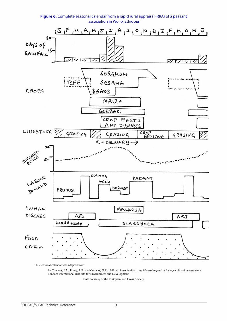
Figure 6. Complete seasonal calendar from a rapid rural appraisal (RRA) of a peasant association in Wollo, Ethiopia
This seasonal calendar was adapted from:
McCracken, J.A.; Pretty, J.N.; and Conway, G.R. 1988. An introduction to rapid rural appraisal for agricultural development. London: International Institute for Environment and Development.
Data courtesy of the Ethiopian Red Cross Society
SQUEAC/SLEAC Technical Reference 10

The SQUEAC method uses a two-stage screening test model:
Stage 1 identifies areas of low and high coverage as well as reasons for coverage failure using routine program data, already available data, quantitative data that may be collected with little additional work, and qualitative data.
Stage 2 confirms the location of areas of high and low coverage and the reasons for coverage failure identified in Stage 1 using small studies, small surveys, small-area surveys.
If appropriate and required, an additional stage may be performed:
Stage 3 provides an estimate of overall program coverage using Bayesian techniques.
SQUEAC consists of a set of tools each of which is designed to identify and investigate coverage and factors influencing coverage.
The tools presented here have been developed and tested in use-studies and by SQUEAC practitioners that have undertaken more than 50 SQUEAC investigations of CMAM programs in many countries in Africa and Asia.
It is expected that new tools will be added and existing tools refined as practitioners gain more experience with the SQUEAC method. A SQUEAC investigation will typically use some (but not all) of the tools described here.
Diverse Tools and Analyses
SQUEAC relies on a diversity of analyses pursued through the use of diverse sources of information, diverse means of collecting information, and diverse methods of analysing information (triangulation). Accuracy and completeness are achieved by investigating coverage and factors influencing coverage in a variety of ways. The ‘truth’ about coverage is approached by a rapid and intelligent accumulation of diverse information, rather than by a single process of dumb statistical replication (although some dumb statistical replication will play a useful role in almost all SQUEAC investigations). Use of routine data, secondary data (e.g., from food-security assessments and nutritional anthropometry surveys), semi-structured interviews, case-histories, informal group discussions, small studies, small surveys, small-area surveys, and the preparation of maps and diagrams all contribute to a progressively accurate and complete analysis of program coverage.
SQUEAC is a semi-structured activity designed to rapidly accumulate new and relevant information about coverage and factors influencing coverage and to develop and test hypotheses about coverage and factors influencing coverage.
SQUEAC/SLEAC Technical Reference 11

SQUEAC is:
• Investigative. SQUEAC is not a survey technique. It is a technique for investigating coverage and factors influencing coverage. A SQUEAC investigation will, if needed, include surveys, but should never be limited to undertaking surveys.
• Iterative. The process of a SQUEAC investigation is not fixed, but is modified as knowledge is acquired. This can be thought of as a process of ‘learning as you go’. New information is used to decide the next steps of the investigation.
• Innovative. There is no standardised SQUEAC method. SQUEAC is a set of tools for investigating coverage and factors influencing coverage. If, when, and how these tools are used depends on the particular setting and the skills of the investigator. Different tools may be used and new tools may be developed as required.
• Interactive. The method collects information through intelligent interaction with program staff, program beneficiaries, and community members using semi-structured interviews, case histories, and informal group discussions.
• Informal. The method uses informal but guided interview techniques as well as formal survey instruments to collect information about coverage and factors influencing coverage.
• In the community. Much of the information used in SQUEAC investigations is collected in the community through interaction with community members. SQUEAC lets you see your program as it is seen by the community.
• Intelligent. Triangulation is a purposeful and intelligent process. Data from different sources and methods are compared with each other. Discrepancies in the data are used to inform decisions about whether to collect further data. If further data collection is required, these discrepancies help determine which data to collect, as well as the sources and methods to be used to collect them.
When done correctly, a SQUEAC investigation will contain all these elements and provide useful information about coverage and factors influencing coverage.
Data Sources and Methods of Analysis: Routine Program Data
The most important item of routine program data is the number of admissions over time. This should be graphed with time on the x axis and number of admissions on the y axis. Since there is likely to be considerable weekly or monthly variation in the number of admissions it is advisable to apply some form of smoothing using, for example, the method of moving averages to the data (Figure 7 and Figure 8). Smoothing time-series data using moving averages is discussed in Appendix 1.
Experience with CMAM programs in a variety of emergency settings shows that programs with reasonable coverage display a distinctive pattern in the plot of admissions over time. Figure 9 shows this pattern over an entire program cycle for an emergency-response program. The number of admissions increases rapidly, falls slightly before stabilising, and finally drops away as the emergency abates and the program is scaled down and approaches closure. Major deviations from this pattern in the absence of evidence of mass migration or significant improvements in the health, nutrition, and food-security situation of the program’s target population indicates a potential problem with a program’s recruitment procedures. For example, Figure 10 shows a plot of admissions over time in an emergency-response CMAM program that had neglected to undertake effective community mobilisation and outreach activities. Admissions initially increased rapidly and then fell away rapidly. Such a pattern is indicative of a program with limited spatial coverage relying on self-referrals. An acceptable pattern was established in this program after effective remedial action was undertaken.
SQUEAC/SLEAC Technical Reference 12

The pattern of admissions in a non-emergency setting is likely to be more complicated and, once the program has been established, should vary with the incidence of SAM in the program’s catchment area (e.g., as in Figure 8). Making sense of the plot of admissions over time in such settings requires information about the probable or expected incidence of SAM. This can be determined using seasonal calendars of human diseases associated with SAM in children (e.g., diarrhoea, fever, and acute respiratory tract infection) and food availability. This information may be available from health and nutrition or food-security assessments (e.g., as in Figure 6). If this information is not already available, it should be collected at the start of the program or during the SQUEAC investigation. Figure 11 shows an example data collection form. Prevalence and incidence data may be available from previous nutritional anthropometry surveys, surveillance systems, and clinic workload returns. Figure 12, for example, shows a plot of admissions over time with seasonal calendars of human diseases and food availability. The pattern of the plot of admissions over time conforms to expectations (i.e., the program treated more cases at times when the incidence of SAM was likely to be high). Deviation from the expected pattern indicates a potential problem with a program’s recruitment procedures.
Figure 7. Plot of program admissions over time (with and without smoothing)
SQUEAC/SLEAC Technical Reference 13
Raw data smoothed using moving medians of span = 3 followed by moving averages of span = 3.
Data courtesy of Concern Worldwide
0 1 2 3 4 5 6 7 8 9 10 11 12 13 14 15 16 17 18 19 20
50
75
100
125
150
Months since start of program
Ad
mis
sion
s
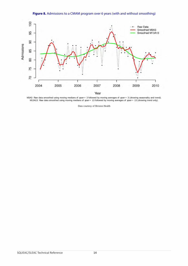
Figure 8. Admissions to a CMAM program over 6 years (with and without smoothing)
M3A3: Raw data smoothed using moving medians of span = 3 followed by moving averages of span = 3 (showing seasonality and trend).M13A13: Raw data smoothed using moving medians of span = 13 followed by moving averages of span = 13 (showing trend only).
Data courtesy of Brixton Health
SQUEAC/SLEAC Technical Reference 14
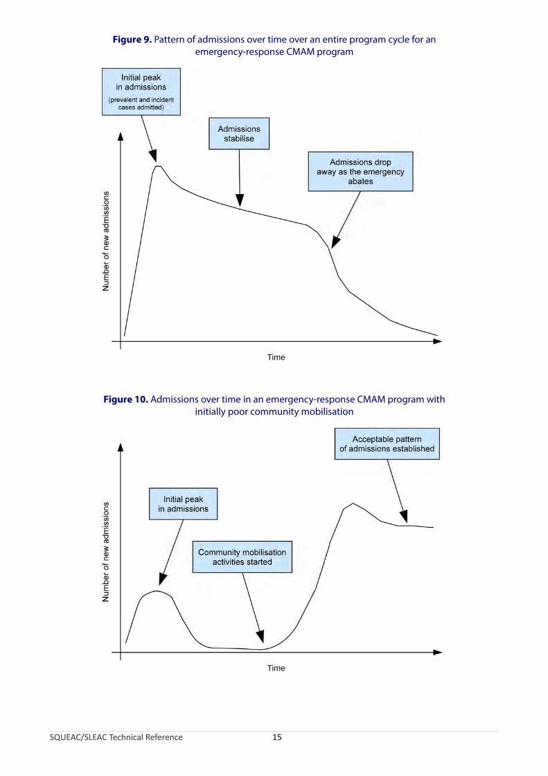
Figure 9. Pattern of admissions over time over an entire program cycle for an emergency-response CMAM program
Time
Figure 10. Admissions over time in an emergency-response CMAM program with initially poor community mobilisation
SQUEAC/SLEAC Technical Reference 15
Time
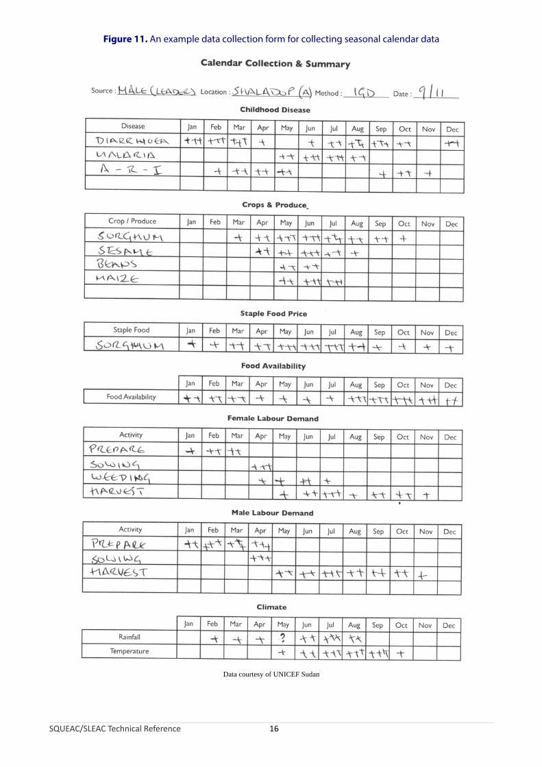
Figure 11. An example data collection form for collecting seasonal calendar data
Data courtesy of UNICEF Sudan
SQUEAC/SLEAC Technical Reference 16

Figure 12. Pattern of CMAM admissions over time with seasonal calendars of human diseases associated with SAM in children and household food availability
SQUEAC/SLEAC Technical Reference 17
Time
Num
ber
of n
ew
ad
mis
sio
ns
Diarrhoea
ARI
Fever Fever
ARI
Fever
Dis
eas
e
Diarrhoea
Foo
d e
ate
n
Plotting admissions over time is useful but ignores the issue of the timeliness of admissions. Children with MUAC below program admission criteria or with nutritional oedema should be in the program. If many of these children are not in the program then program coverage will be low. These children can be divided into two groups:
• Children that meet program admission criteria but never get admitted to the program. These children either recover outside of the program or die. It is possible to identify some of these children using referral monitoring or surveys.
• Children that are admitted to the program, but only after they have met program admission criteria for a considerable period of time. These children are late admissions and can be identified using data that are usually recorded on the beneficiary record card.
Late admissions are direct coverage failures (because they will have been non-covered SAM cases for a considerable period of time before admission) but they also affect coverage indirectly. Late admission is associated with the need for inpatient care, longer treatment, defaulting, and poor treatment outcomes (e.g., death). These can lead to poor opinions of the program circulating in the host population, which may lead to more late presentations and admissions and a cycle of negative feedback may develop (Figure 13).
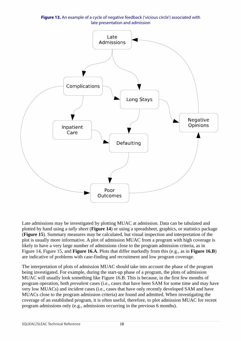
Figure 13. An example of a cycle of negative feedback (‘vicious circle’) associated with late presentation and admission
SQUEAC/SLEAC Technical Reference 18
Late admissions may be investigated by plotting MUAC at admission. Data can be tabulated and plotted by hand using a tally sheet (Figure 14) or using a spreadsheet, graphics, or statistics package (Figure 15). Summary measures may be calculated, but visual inspection and interpretation of the plot is usually more informative. A plot of admission MUAC from a program with high coverage is likely to have a very large number of admissions close to the program admission criteria, as in Figure 14, Figure 15, and Figure 16.A. Plots that differ markedly from this (e.g., as in Figure 16.B) are indicative of problems with case-finding and recruitment and low program coverage.
The interpretation of plots of admission MUAC should take into account the phase of the program being investigated. For example, during the start-up phase of a program, the plots of admission MUAC will usually look something like Figure 16.B. This is because, in the first few months of program operation, both prevalent cases (i.e., cases that have been SAM for some time and may have very low MUACs) and incident cases (i.e., cases that have only recently developed SAM and have MUACs close to the program admission criteria) are found and admitted. When investigating the coverage of an established program, it is often useful, therefore, to plot admission MUAC for recent program admissions only (e.g., admissions occurring in the previous 6 months).

Figure 14. Admission MUAC tabulated/plotted by hand using a tally sheet for a CMAM program admitting on MUAC < 115 mm
Data courtesy of World Vision International
SQUEAC/SLEAC Technical Reference 19

Figure 15. Admission MUAC plotted using a statistics package for a CMAM program admitting on MUAC < 110 mm
Data courtesy of Save the Children (USA) and the Friedman School of Nutrition Science and Policy (Tufts University)
SQUEAC/SLEAC Technical Reference 20
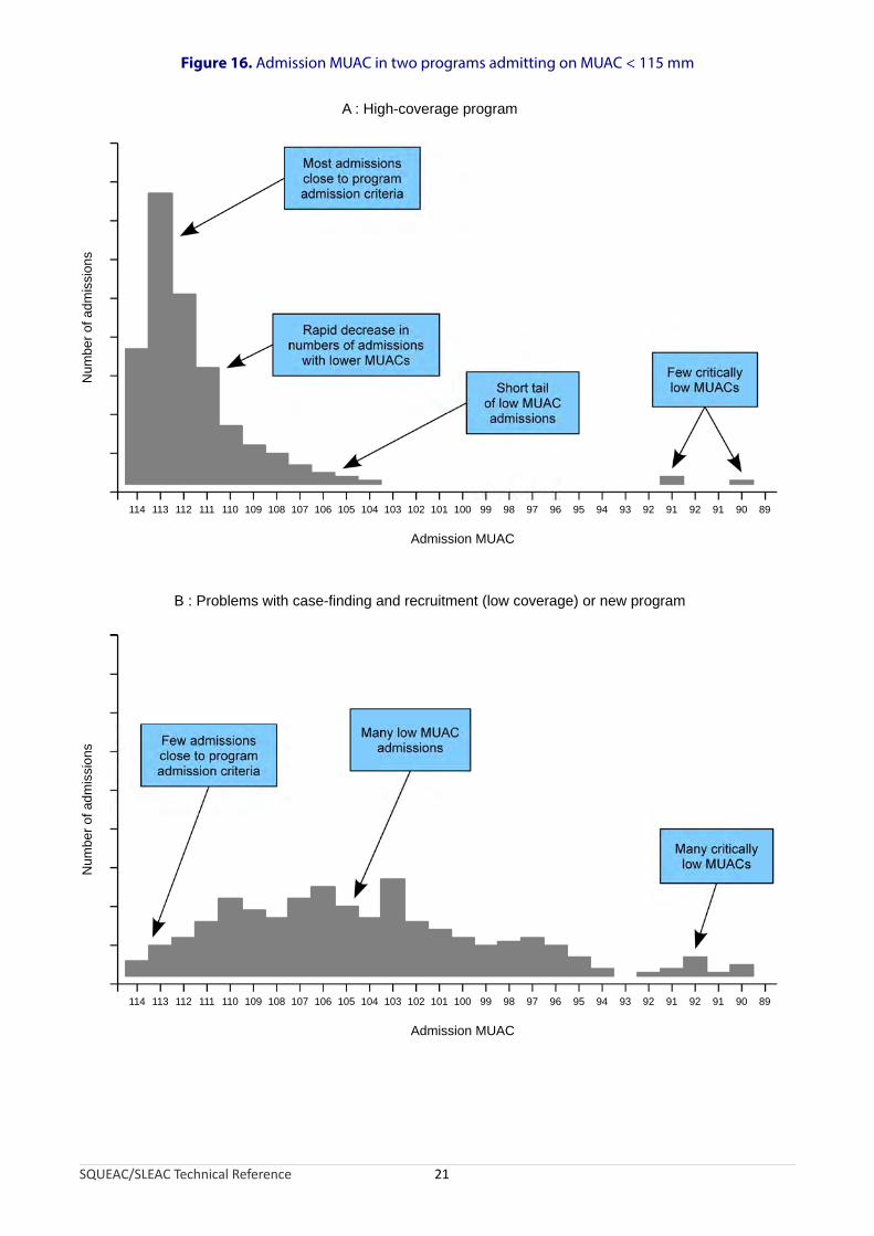
Figure 16. Admission MUAC in two programs admitting on MUAC < 115 mm
SQUEAC/SLEAC Technical Reference 21
114 113 112 111 110 109 108 107 106 105 104 103 102 101 100 99 98 97 96 95 94 93 92 91 92 91 90 89
Admission MUAC
Num
ber
of a
dmis
sion
s
114 113 112 111 110 109 108 107 106 105 104 103 102 101 100 99 98 97 96 95 94 93 92 91 92 91 90 89
Admission MUAC
Num
ber
of a
dm
issi
ons
A : High-coverage program
B : Problems with case-finding and recruitment (low coverage) or new program

Another way of investigating late admissions is to calculate the proportion of program beneficiaries requiring inpatient care at admission:
Number of program beneficaries requiring inpatient care at admission × 100Total number of inpatient and outpatient admissions
Interpretation of the proportion of program beneficiaries requiring inpatient care at admission should also take into account the phase of the program being investigated. The proportion of program beneficiaries requiring inpatient care at admission is likely to be high during the start-up phase of a program. In an established program, however, the proportion of program admissions requiring inpatient care should not exceed 5%.
Note that the calculation of the proportion of program beneficiaries requiring inpatient care at admission uses the number of program beneficiaries requiring inpatient care at admission rather than the number of program beneficiaries admitted to inpatient care as the numerator. This is because many carers may not accept a referral to an inpatient facility.
The proportion of program beneficiaries requiring inpatient care at admission may also be analysed (classified) using the simplified Lot Quality Assurance Sampling (LQAS) classification technique presented later in this section.
An investigation of late admissions will usually identify some very late admissions (e.g., the three cases with MUAC < 90 mm in Figure 14). Children that remain untreated for such long periods with declining nutritional status should be treated as critical incidents. Investigation of critical incidents often reveals useful information about program performance. For example, a SQUEAC investigation of a CMAM program in Bangladesh reported:
A child was admitted to the program with a MUAC of 82 mm. The mother of this case had moved (within the program catchment area) to live with her father because of family problems. While at her grandfather’s house, the child developed diarrhoea with fever and rapid weight loss. The child spent 12 days in the local hospital before being discharged with a MUAC approaching 82 mm. The community nutrition volunteers at the grandfather’s home union and the mother’s home union were not informed by the hospital. Program staff were also not informed by the hospital. The case was, however, picked up by the community nutrition volunteer at the grandfather’s home union, referred to the community nutrition volunteer at the case’s home union, and admitted to the program. The referring community nutrition volunteer also informed program staff of the referral.
In this example, the investigation of a critical incident revealed good communications within the program but a problem with the interface between the local hospital and the program and prompted further investigation into the interface between the local hospital and the program.
Examining the duration of the treatment episode (i.e., the time from admission to discharge) may also provide useful information about program coverage. The duration of the treatment episode is sometimes called the ‘length of stay’.
Long treatment episodes may be due to late admission or poor adherence to the CMAM treatment protocol by program staff (e.g., failure to give a systemic antimicrobial, RUTF stock-outs) and beneficiaries (e.g., intra-household sharing of RUTF, lack of continuity of care). Programs with long treatment episodes tend to be unpopular with beneficiaries and suffer from late treatment seeking and high levels of defaulting (both of which are failures of coverage).
SQUEAC/SLEAC Technical Reference 22
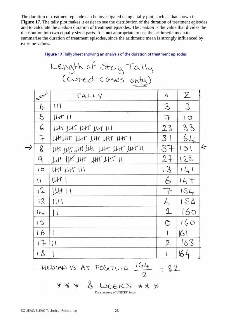
The duration of treatment episode can be investigated using a tally plot, such as that shown in Figure 17. The tally plot makes it easier to see the distribution of the duration of treatment episodes and to calculate the median duration of treatment episodes. The median is the value that divides the distribution into two equally sized parts. It is not appropriate to use the arithmetic mean to summarise the duration of treatment episodes, since the arithmetic mean is strongly influenced by extreme values.
Figure 17. Tally sheet showing an analysis of the duration of treatment episodes
Data courtesy of UNICEF Sudan
SQUEAC/SLEAC Technical Reference 23

Higher coverage programs tend to have a median duration of treatment episodes of less than or equal to about 8 weeks.
When examining the duration of treatment episodes you should restrict the analysis to planned discharges (i.e., include cases discharged as cured and as non-responders in the analysis, but exclude defaulters and transfers to other programs from the analysis). The analysis presented in Figure 17, for example, was restricted to cured cases only.
The interpretation of plots and summaries of duration of treatment episodes should take into account the phase of the program being investigated. For example, during the start-up phase of a program, there may be many long duration treatment episodes. This is because, in the first few months of program operation, both prevalent (old) and incident (new) cases are found and admitted. When investigating the coverage of an established program, it is often useful, therefore, to plot and summarise duration of treatment for recent discharges only (e.g., discharges occurring in the previous 6 months).
Plots of admissions over time and admission MUAC can reveal potential problems with a program’s recruitment procedures, but ignore the problem of defaulters. Defaulters are children that have been admitted to the program but leave the program without being formally discharged, without being transferred to another service, or without having died. Defaulters are, therefore, children that should be in the program but are not in the program. This means that high defaulting rates are associated with low program coverage. Standard program indicator graphs should show a consistently low rate of defaulting. Figure 18 shows a standard program indicator graph from a CMAM program. This graph shows an increasing defaulting rate. This was due to the program having too few sites. More cases were found and admitted as the program’s outreach activities were expanded, but more of these cases defaulted after the initial visit because beneficiaries and carers had to travel too far to access services. Note that deaths in Figure 18 show a similar pattern to defaulters. The bulk of these deaths were in late admissions from communities furthest from program sites.
SQUEAC/SLEAC Technical Reference 24

Figure 18. Standard therapeutic feeding program indicator graph
Data courtesy of Concern Worldwide
In some programs, defaulting rates may vary over time. This will usually be due to a deterioration in the security situation, meteorological conditions (e.g., difficulties travelling in rainy or hot seasons), or patterns of labour demand. Figure 19, for example, shows a plot of the defaulting rate over time with a seasonal calendar of household labour demands. In this example, defaulting is associated with household labour demands. Such a problem could be corrected by reducing the cost of attendance by, for example, opening additional program sites, using mobile clinics, reducing contact frequency from weekly to fortnightly contact, or reducing waiting times at program sites. Plots of defaulting rates over time should present defaults as a proportion of all program exits, as in Figure 18. As with admissions data, it is advisable to apply smoothing to the raw data before plotting.
SQUEAC/SLEAC Technical Reference 25
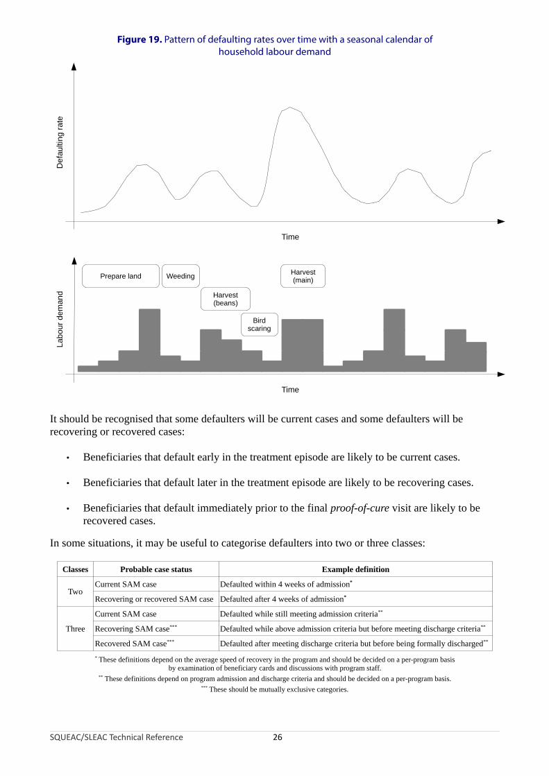
Figure 19. Pattern of defaulting rates over time with a seasonal calendar ofhousehold labour demand
Time
De
fau
ltin
g ra
teL
abo
ur d
eman
d
Prepare land Harvest(main)Weeding
Harvest(beans)
Birdscaring
Time
It should be recognised that some defaulters will be current cases and some defaulters will be recovering or recovered cases:
• Beneficiaries that default early in the treatment episode are likely to be current cases.
• Beneficiaries that default later in the treatment episode are likely to be recovering cases.
• Beneficiaries that default immediately prior to the final proof-of-cure visit are likely to be recovered cases.
In some situations, it may be useful to categorise defaulters into two or three classes:
Classes Probable case status Example definition
Current SAM case Defaulted within 4 weeks of admission*
TwoRecovering or recovered SAM case Defaulted after 4 weeks of admission*
Current SAM case Defaulted while still meeting admission criteria**
Three Recovering SAM case*** Defaulted while above admission criteria but before meeting discharge criteria**
Recovered SAM case*** Defaulted after meeting discharge criteria but before being formally discharged**
* These definitions depend on the average speed of recovery in the program and should be decided on a per-program basisby examination of beneficiary cards and discussions with program staff.
** These definitions depend on program admission and discharge criteria and should be decided on a per-program basis.*** These should be mutually exclusive categories.
SQUEAC/SLEAC Technical Reference 26
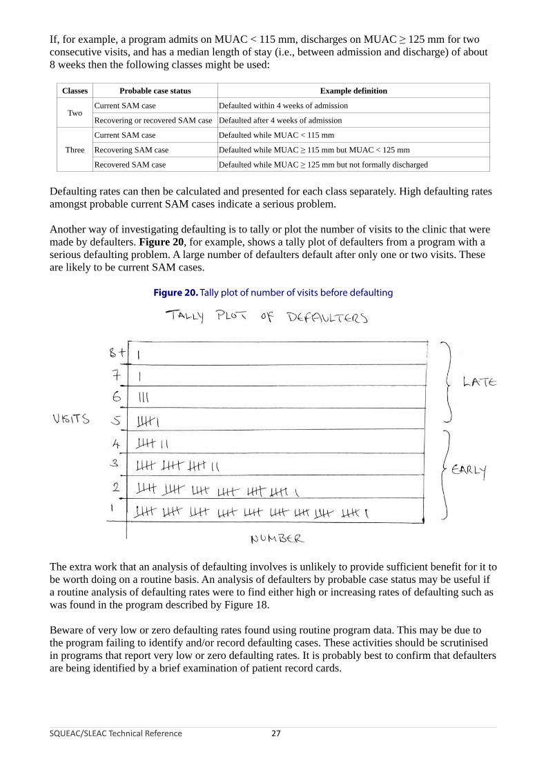
If, for example, a program admits on MUAC < 115 mm, discharges on MUAC ≥ 125 mm for two consecutive visits, and has a median length of stay (i.e., between admission and discharge) of about 8 weeks then the following classes might be used:
Classes Probable case status Example definition
Current SAM case Defaulted within 4 weeks of admissionTwo
Recovering or recovered SAM case Defaulted after 4 weeks of admission
Current SAM case Defaulted while MUAC < 115 mm
Three Recovering SAM case Defaulted while MUAC ≥ 115 mm but MUAC < 125 mm
Recovered SAM case Defaulted while MUAC ≥ 125 mm but not formally discharged
Defaulting rates can then be calculated and presented for each class separately. High defaulting rates amongst probable current SAM cases indicate a serious problem.
Another way of investigating defaulting is to tally or plot the number of visits to the clinic that were made by defaulters. Figure 20, for example, shows a tally plot of defaulters from a program with a serious defaulting problem. A large number of defaulters default after only one or two visits. These are likely to be current SAM cases.
Figure 20. Tally plot of number of visits before defaulting
The extra work that an analysis of defaulting involves is unlikely to provide sufficient benefit for it to be worth doing on a routine basis. An analysis of defaulters by probable case status may be useful if a routine analysis of defaulting rates were to find either high or increasing rates of defaulting such as was found in the program described by Figure 18.
Beware of very low or zero defaulting rates found using routine program data. This may be due to the program failing to identify and/or record defaulting cases. These activities should be scrutinised in programs that report very low or zero defaulting rates. It is probably best to confirm that defaulters are being identified by a brief examination of patient record cards.
SQUEAC/SLEAC Technical Reference 27

The home location of the beneficiary is usually recorded on the beneficiary record card. Mapping the home locations of beneficiaries attending each program site is a simple way of defining the actual (rather than the intended) catchment area of each program site. Figure 21, for example, shows the home location of each beneficiary attending a program site who was admitted to the program in the previous 2 months. This plot suggests that the program has limited spatial coverage, with coverage restricted to areas close to program sites or along the major roads leading to program sites.
Mapping is also a useful way of assessing outreach activities. Figure 22, for example, shows the villages visited by program outreach workers in the previous 2 months. The pattern is similar to that observed on the map of the home locations of beneficiaries attending the program site (Figure 21) with outreach activities having limited spatial coverage (i.e., restricted to areas close to program sites or along the major roads leading to program sites).
Figure 21. Home locations of program beneficiaries
Size of symbol is proportional to the number of admissions from each location.
Intended catchment
Major road
Towns and villages
Program site
Legend
Home locations
SQUEAC/SLEAC Technical Reference 28

Figure 22. Villages visited by program outreach workers in the previous 2 months
SQUEAC/SLEAC Technical Reference 29
Intended catchment
Major road
Towns and villages
Program site
Legend
Outreach visits
A complementary way of assessing outreach activities is to record the dates of outreach visits against a complete list of villages in the program’s intended catchment area (Figure 23). The performance categories in Figure 23 corresponds to:
Poor : Zero, one, or two outreach visits in the previous 6 months
OK : Three or four outreach visits in the previous 6 months
Good : Five or more outreach visits in the previous 6 months
Other categories could be used (e.g., based on the date of the most recent outreach visit) but it is usually best to work with three categories.
Mapping and tabulation complement each other. Maps allow simple spatial analysis (e.g., Figure 22). Tables allow more complicated analyses. For example, Figure 23 shows an analysis of outreach activities by place and time that:
• Presents a calender of recent outreach activities• Identifies coverage failures localised in both place and time• Shows level of success achieved by place• Assesses the performance of outreach teams
It should be noted that, despite the multi-variable sophistication of the tabular analysis presented in Figure 23, it fails to make explicit that outreach activities were restricted to areas close to program sites or along the major roads leading to program sites. Mapping and tabulation complement each other.
From Figure 22 and Figure 23 it can be seen that this program has both poor spatial and temporal coverage of outreach activities. Maps or lists of the home locations of community-based volunteers (CBVs) and community health workers (CHWs) provide similar information for programs that use CBVs and CHWs for case-finding and carer support and mentoring. The spatial and/or temporal coverage of outreach activities may also be analysed using the simplified LQAS classification technique presented later in this section.

Figure 23. Dates of outreach visits against a complete list of villages
SQUEAC/SLEAC Technical Reference 30
Month of visit
Village Team Jun Jul Aug Sep Oct NovNumber
of visitsLevel ofsuccess
Bene Mukenda A 4/6/10 5/7/10 13/8/10 3/9/10 8/10/10 5/11/10 6 Good
Bwanaali A 4/6/10 13/8/10 3/9/10 8/10/10 5/11/10 5 Good
Bwese A 11/6/10 30/7/10 24/8/10 3 OK
Kasha A 11/6/10 30/7/10 27/8/10 24/9/10 4 OK
Kingombe A 4/6/10 5/7/10 13/8/10 3/9/10 15/10/10 19/11/10 6 Good
Kiyana A 11/6/10 9/7/10 6/8/10 3/9/10 22/10/10 5 Good
Lumanisha A 18/6/10 1 Poor
Mupuluzi A 23/7/10 20/8/10 2 Poor
Mushanyondo A 4/6/10 9/7/10 6/8/10 10/9/10 15/10/10 26/11/10 6 Good
Muyumba A 25/6/10 1 Poor
Muzee A 18/6/10 1 Poor
Mwaka A 4/6/10 2/7/10 13/8/10 3 OK
Mwaza A 4/6/10 9/7/10 13/8/10 17/9/10 19/11/10 5 Good
Mwendebule A 18/6/10 23/7/10 2 Poor
Kamangu B 18/6/10 1 Poor
Kandolu B 0 Poor
Kasangati B 0 Poor
Kikumbi B 18/6/10 1 Poor
Lwanga B 25/6/10 1 Poor
Mbaruku B 0 Poor
Milambi B 18/6/10 9/10/10 2 Poor
Misuyu B 4/6/10 1 Poor
Mubonga B 0 Poor
Munganga B 11/6/10 1 Poor
Mwezia B 25/6/10 23/7/10 2 Poor
Note: Tables like this are useful for analysing spatial data over time. In this table:
Location (i.e., village) is shown in rows.
Time (i.e., month) is shown on in columns.
Empty cells represent coverage failures at particular places at particular times.
It is possible to add more dimensions to the analysis. In this table, the numbers of visits to each village are tallied and used to classify levels of success achieved over the entire reporting period (see text). Analysis by outreach team, for example, is possible. Team A is doing better than Team B:
Team A Team B
Mean number of visits 3.50 0.82
Level ofsuccess
Good 6 (43%) 0 (0%)
OK 3 (21%) 0 (0%)
Poor 5 (36%) 11 (100%)
This analysis is simpler when the table is sorted by outreach team (as above).

It is also useful to map the home locations of defaulting cases. Figure 24, for example, shows the home locations of beneficiaries that defaulted in the previous 2 months. Most defaulting cases come from villages far from the program site, suggesting that lack of proximity to services (either to the program site or to outreach and support services) is a leading cause of defaulting. It may also be useful to record and map cases that did not attend (DNA) the program despite having been referred to the program. DNA cases can be identified by referral monitoring (see below). Follow-up of defaulting and DNA cases (with home visits) should also be undertaken to identify reasons for defaulting and non-attendance.
Figure 24. Home locations of program beneficiaries that defaulted in the previous 2 months
SQUEAC/SLEAC Technical Reference 31
Intended catchment
Major road
Towns and villages
Program site
Legend
Defaulting cases
Mapping does not require the use of sophisticated mapping or geographical information system (GIS) software packages or the use of Global Positioning System (GPS) receivers. All of the mapping work outlined in this section can be performed with a paper map of useful scale, transparent plastic sheets, adhesive masking tape (masking tape can be written on and is easy to remove, which reduces damage to paper maps), Post-it™ notes, and marker pens. Figure 25, for example, shows a coverage assessment worker mapping the home locations of admissions and defaulters (labelled ‘ABANDONS’) on a map covered by a transparent plastic sheet. The use of transparent plastic sheets, masking tape, and Post-it™ notes preserves paper maps for later coverage assessments or other purposes. Recording different data on separate transparent plastic sheets and overlaying these on the map is very useful because it allows several dimensions of data to be compared and analysed at the same time.

Figure 25. A coverage assessment worker mapping the home locations of program beneficiaries
Photograph courtesy of Save the Children (Canada)
An alternative to mapping is to use lists and tables. This approach is useful for analysing spatial data over time. This is illustrated in Figure 23, which shows how a table can be used to identify gaps (in both space and time) in program outreach activities.
Lists and tables are also useful when maps are not available or where mapping may prove difficult, such as in urban, peri-urban, or ‘shanty’ areas. For example, Table 1 shows how a table can be used to investigate the effect of distance (travel time) on admissions and defaulting in an urban program. The data in Table 1 suggests that, in this program, distance has an effect on both admissions (higher close to the clinic) and defaulting (higher further from the clinic). Listing is a useful and simple way of identifying locations where coverage is likely to be poor (i.e., locations from which there are very few or no admissions) or defaulting is likely to be high (see Table 2). This approach requires you to have a complete list of locations (e.g., villages) in the catchment area of a program or program site.
Table 1. Use of a table to investigate the effect of distance on admissions and defaulting in the previous month in a single clinic catchment area
Healthzone
Distance(time-to-travel)
Admissions DefaultersGrouped distance
(time-to-travel)Admissions Defaulters
DefaultersAdmissions × 100
2 10 minutes 3 1
1
4
5
15 minutes
2 0
1 1
2 2
6
720 minutes
0 0
3 0
≤ 20 minutes 11 4 36.00%
3 30 minutes 0 0
8
945 minutes
1 0
0 0
10 60 minutes 0 0
11 90 minutes 1 1
> 20 minutes 2 1 50%
Data courtesy of Lusaka District Health Management Team
SQUEAC/SLEAC Technical Reference 32
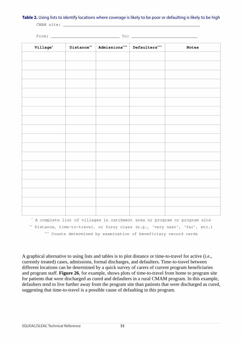
Table 2. Using lists to identify locations where coverage is likely to be poor or defaulting is likely to be high
CMAM site: ________________________________________________________
From: ____________________________ To: ___________________________
Village* Distance** Admissions*** Defaulters*** Notes
* A complete list of villages in catchment area or program or program site
** Distance, time-to-travel, or fuzzy class (e.g., ‘very near’, ‘far’, etc.)
*** Counts determined by examination of beneficiary record cards
A graphical alternative to using lists and tables is to plot distance or time-to-travel for active (i.e., currently treated) cases, admissions, formal discharges, and defaulters. Time-to-travel between different locations can be determined by a quick survey of carers of current program beneficiaries and program staff. Figure 26, for example, shows plots of time-to-travel from home to program site for patients that were discharged as cured and defaulters in a rural CMAM program. In this example, defaulters tend to live further away from the program site than patients that were discharged as cured, suggesting that time-to-travel is a possible cause of defaulting in this program.
SQUEAC/SLEAC Technical Reference 33
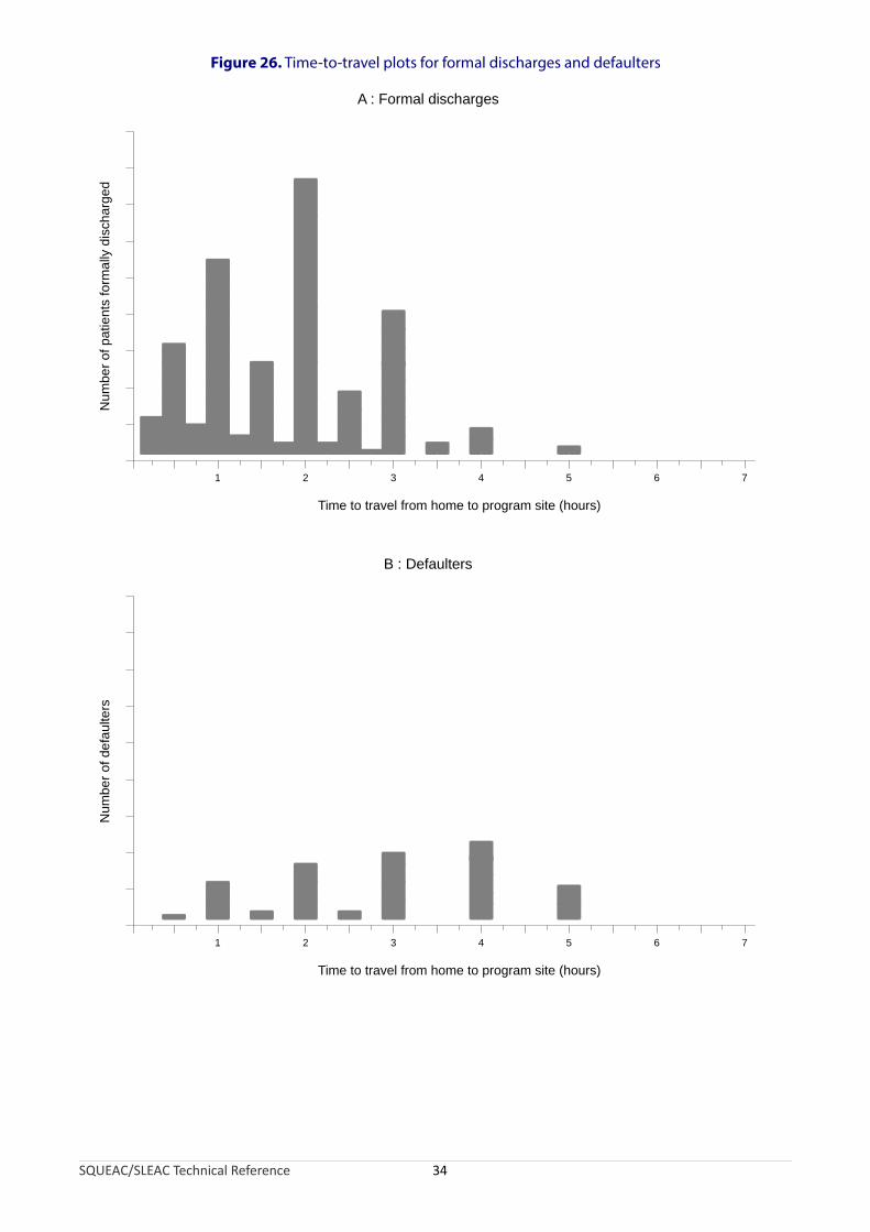
Figure 26. Time-to-travel plots for formal discharges and defaulters
SQUEAC/SLEAC Technical Reference 34
1 2 3 4 5 6
Time to travel from home to program site (hours)
Num
ber
of p
atie
nts
form
ally
dis
char
ge
dA : Formal discharges
1 2 3 4 5 6
Time to travel from home to program site (hours)
Num
ber
of d
efa
ulte
rs
B : Defaulters
7
7

Plotting time-to-travel is also useful for checking assumptions regarding program site catchment areas. Figure 27 shows a plot of the time-to-travel for active (i.e., currently treated) cases for a single program site in a rural CMAM program. When this program was established, it was assumed that beneficiaries would attend from as far as 18 km away from this program site. Examination of Figure 27 reveals that this assumption was probably optimistic. Assuming that a mother carrying a sick child over rough and forested terrain can sustain a walking speed of about 3 km/hour, the actual boundary of the effective (actual) catchment area for the program site was unlikely to extend beyond about 12 km from the program site.
Figure 27. Time-to-travel for active (currently treated) cases for a single program site in a rural CMAM program
Data courtesy National Food and Nutrition Council of Zambia
SQUEAC/SLEAC Technical Reference 35

It is important to realise that shrinking the distance from the program site to the boundary of the catchment area can have a large effect on the area (A) covered by the program site:
18 km
12 km
8 km6 km
A=1018km2 A=452km2 A=201km 2 A=113km2
The intended catchment area of the program site illustrated in Figure 27 was about:
AreaIntended = π r 2 = π × 182 = π × 324 = 1018km 2
Figure 27 shows that no currently treated case came from villages more than 4 hours’ walk (i.e., about 12 km) from the program site. This means that the effective catchment area of the program site is unlikely to have extended more than about 12 km from the program site. The effective (actual) catchment area of the program site illustrated in Figure 27 was about:
Area 2 2 2Effective = πr = π × 12 = π × 144 = 452km
The effective catchment area includes:
AreaEffective 452× 100= × 100= 44.4%AreaIntended 1018
of the intended catchment area. This means that more than half of the intended catchment area for this program site was probably not covered.
When examining plots of time-to-travel, such as those shown in Figure 27, it is important to consider the pattern of settlement in the intended program site catchment area. This can be used to create an expected distribution of time-to-travel that can be compared to the observed distribution of time-to-travel. The expected distribution need only be approximate. Discrepancies between the shapes of the expected and the observed distributions are suggestive of problems with program coverage. In this approach, ‘expected distribution’ means the shape of the distribution we would expect to see if coverage were spatially even and the comparison is between the shapes of the expected and observed distributions. The expected distribution shown in Figure 28, for example, was created using a simple count of villages within each hour-wide ring (with the main town where the program site is located being counted as four villages) and assumes that villages were similar in population size and the incidence of SAM did not vary much over the program site’s intended catchment area.
SQUEAC/SLEAC Technical Reference 36

Figure 28. Expected and observed pattern for time-to-travel for active (currently treated) cases within the intended catchment area of a program site in a rural CMAM program
Comparing the shapes of the expected and observed distribution of active cases in Figure 28 reveals that recruitment tends to decrease with increasing distance, when it is expected to increase with increasing distance (because the number of villages in the intended catchment area increases with increasing distance from the program site). This suggests that coverage is likely to be poor in villages located more than about 3 hours’ walk from the program site.
SQUEAC/SLEAC Technical Reference 37
0 to 1 hour
1 to 2 hours
2 to 3 hours
3 to 4 hours
4 to 5 hours
Time-to-travel
4
2
6
6
9
Villages
0-1 1-2 2-3 3-4 4-5
0
1
2
3
4
5
6
7
8
9
1 0
Expected Distribution
Time-to-travel
Nu
mb
er
of
vill
ag
es
0-1 1-2 2-3 3-4 4-5
0
1
2
3
4
5
6
7
8
9
1 0
Observed Distribution
Time-to-travel
Nu
mb
er
of
ca
se
s
Rings are spaced about 1 hour's travelling time apart
Count villages in each ring
Town countedas four villages
Compare the shapesof the two distributions
Village counts
Counts taken fromroutine program data
Approximate boundary ofintended clinic catchment area
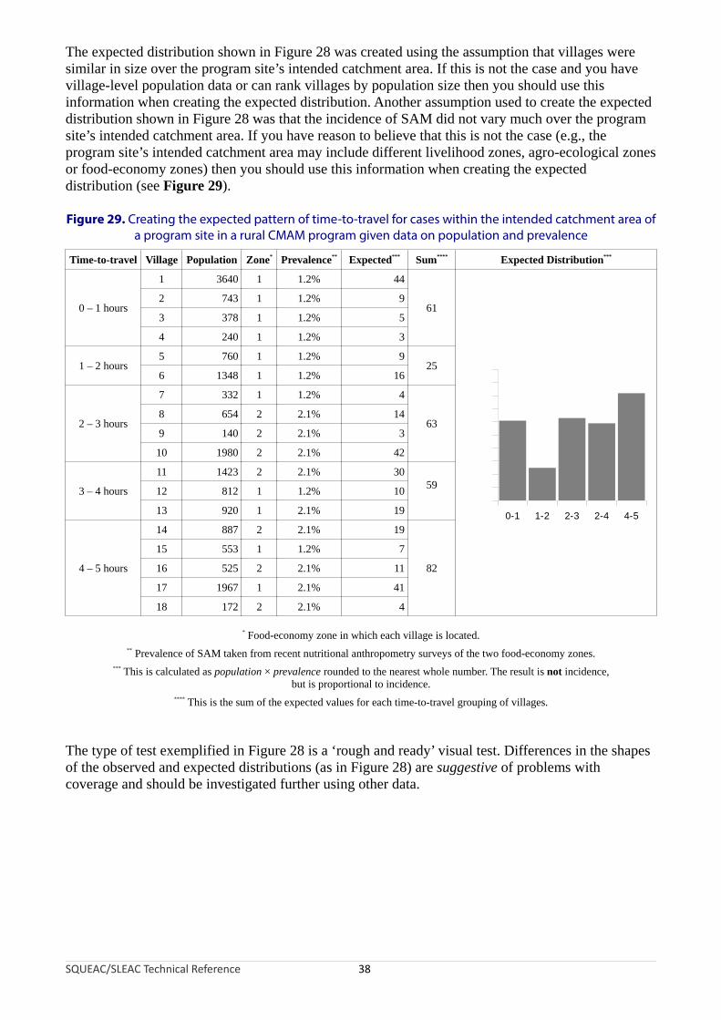
The expected distribution shown in Figure 28 was created using the assumption that villages were similar in size over the program site’s intended catchment area. If this is not the case and you have village-level population data or can rank villages by population size then you should use this information when creating the expected distribution. Another assumption used to create the expected distribution shown in Figure 28 was that the incidence of SAM did not vary much over the program site’s intended catchment area. If you have reason to believe that this is not the case (e.g., the program site’s intended catchment area may include different livelihood zones, agro-ecological zones or food-economy zones) then you should use this information when creating the expected distribution (see Figure 29).
Figure 29. Creating the expected pattern of time-to-travel for cases within the intended catchment area of a program site in a rural CMAM program given data on population and prevalence
Time-to-travel Village Population Zone* Prevalence** Expected*** Sum**** Expected Distribution***
0 – 1 hours
1 3640 1 1.2% 44
61
0-1 1-2 2-3 2-4 4-5
0
10
20
30
40
50
60
70
80
90
100
2 743 1 1.2% 9
3 378 1 1.2% 5
4 240 1 1.2% 3
1 – 2 hours5 760 1 1.2% 9
256 1348 1 1.2% 16
2 – 3 hours
7 332 1 1.2% 4
638 654 2 2.1% 14
9 140 2 2.1% 3
10 1980 2 2.1% 42
3 – 4 hours
11 1423 2 2.1% 3059
12 812 1 1.2% 10
13 920 1 2.1% 19
4 – 5 hours
14 887 2 2.1% 19
82
15 553 1 1.2% 7
16 525 2 2.1% 11
17 1967 1 2.1% 41
18 172 2 2.1% 4
* Food-economy zone in which each village is located.** Prevalence of SAM taken from recent nutritional anthropometry surveys of the two food-economy zones.
*** This is calculated as population × prevalence rounded to the nearest whole number. The result is not incidence,but is proportional to incidence.
**** This is the sum of the expected values for each time-to-travel grouping of villages.
The type of test exemplified in Figure 28 is a ‘rough and ready’ visual test. Differences in the shapes of the observed and expected distributions (as in Figure 28) are suggestive of problems with coverage and should be investigated further using other data.
SQUEAC/SLEAC Technical Reference 38

Experience with CMAM programs shows that the distance or time that carers are willing or able to walk to access services varies greatly between settings. A simple way of estimating this distance is to identify hamlets, villages, and towns on a map:
Typeof place
Populationrange* Features
Hamlet < 1,000 Very small local market or no market
Village 1,000 – 4,000Market and small shops serving the village and the surrounding hamlets
Town > 4,000Large market, many shops (some specialised), guest houses, bus station, government offices
* These ranges may need to be adjusted to match local circumstances.
Then, measure the distances (d) between the neighbouring villages and towns with markets and calculate the mean (average) of these distances:
Mean distance = ∑ d
n
where:
∑ d : Sum of the distances between neighbouring villages and towns with markets
n : The number of distances between neighbouring villages and towns with markets
The distance that carers are willing or able to walk to access services will be approximately half of this mean distance. A worked example of this ‘half-distance between markets’ approach is shown in Figure 30.
SQUEAC/SLEAC Technical Reference 39
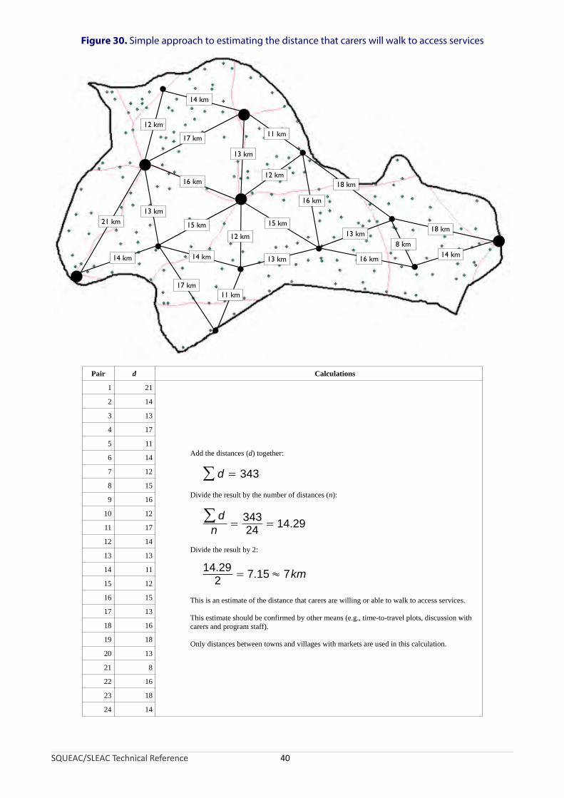
Figure 30. Simple approach to estimating the distance that carers will walk to access services
Pair d Calculations
1 21
Add the distances (d) together:
∑ d = 343
Divide the result by the number of distances (n):
∑ dn
= 34324
= 14.29
Divide the result by 2:
14.29
2= 7.15≈ 7km
This is an estimate of the distance that carers are willing or able to walk to access services.
This estimate should be confirmed by other means (e.g., time-to-travel plots, discussion with carers and program staff).
Only distances between towns and villages with markets are used in this calculation.
2 14
3 13
4 17
5 11
6 14
7 12
8 15
9 16
10 12
11 17
12 14
13 13
14 11
15 12
16 15
17 13
18 16
19 18
20 13
21 8
22 16
23 18
24 14
21 km
14 km
17 km11 km
14 km
13 km
12 km
17 km
14 km
16 km
13 km
18 km
14 km8 km
18 km
16 km
15 km
13 km
12 km
11 km
13 km
16 km
15 km
12 km
SQUEAC/SLEAC Technical Reference 40

The half-distance between markets approach should be used to provide a first estimate only. This estimate should be confirmed by other means (e.g., time-to-travel plots, discussion with carers and program staff). It is very important that the cultural and security context are taken into consideration. For example:
• In some settings, women may not engage in trade or may not engage in trade outside of their home community. This often means that women are reluctant to travel far from their home community in order to access CMAM services.
• In other settings, women must be accompanied by a male family member when they leave their immediate neighbourhood.
• In other settings, it may be dangerous for women to leave their home community.
The half-distance between markets approach may overestimate the distance or time that carers are willing or able to walk to access services in such settings. The estimate should, therefore, always be confirmed by other sources and methods.
A useful way to confirm the results from the half-distance between markets approach is to use group discussions with carers to find the ranges of time-to-travel or distance associated with descriptions such as ‘very near’, ‘near’, ‘not far’, ’not near’, ‘far’, and ‘very far’ and to plot these as as fuzzy numbers:
very not notnear far very far
near far near
0 5 10 15 20 30 60
Time-to-travel (minutes)
In this example, the boundary between far and very far (i.e., just under one hour’s walk) is the probable limit of a program site’s effective catchment area.
Data on program site catchment areas collected using one or more of the suggested methods allows you to map the probable spatial coverage of a program. In Figure 31, for example, the large filled circles around the program sites have a radius of approximately 7 km. This is the distance found by the half-distance between markets approach applied to the program area. This is also the distance that could be comfortably walked in about one-and-a-half hours by a woman carrying a sick child (confirmed by interviews with carers at program sites, program staff, and CBVs) and was consistent with time-to-travel plots of recent program admissions. It is clear from Figure 31 that a large proportion of the population resides a considerable distance from program sites and that coverage is likely to be very low in areas that are distant from program sites. This hypothesis was confirmed by small-area surveys.
SQUEAC/SLEAC Technical Reference 41
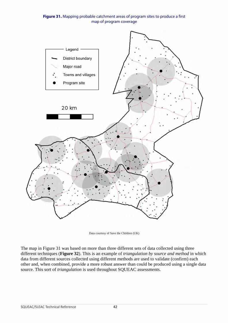
Figure 31. Mapping probable catchment areas of program sites to produce a first map of program coverage
Data courtesy of Save the Children (UK)
The map in Figure 31 was based on more than three different sets of data collected using three different techniques (Figure 32). This is an example of triangulation by source and method in which data from different sources collected using different methods are used to validate (confirm) each other and, when combined, provide a more robust answer than could be produced using a single data source. This sort of triangulation is used throughout SQUEAC assessments.
SQUEAC/SLEAC Technical Reference 42

Figure 32. Triangulation by source and method used to produce the map shown in Figure 31
SQUEAC/SLEAC Technical Reference 43
Interviewswith carers
Time-to-travelplots
Half-distancebetween markets
Probablespatial pattern
of coverage
Interviewswith CBVs
Interviewswith program
staff
Referrals that do not attend the program (DNA referrals) are, like defaulters, children that should be in the program but are not in the program. DNA referrals are also more likely than defaulters to be current cases. This means that high DNA rates are associated with low program coverage. DNA rates can be calculated by monitoring referrals. Mapping of DNA cases can provide information about problems of proximity to services and other barriers to service access and uptake that may also be spatially distributed (e.g., ethnic or religious groups). Follow-up of DNA cases with home visits should be undertaken to identify reasons for non-attendance.
CBVs often have low levels of literacy and numeracy. This means that a different approach to referral monitoring may have to be adopted in programs that use CBVs instead of (or as well as) program extension workers and/or CHWs. One approach is to use ‘cloakroom tickets’ or ‘raffle tickets’ for referral slips (Figure 33). These have two unique identifying numbers (which may be used to identify the referring CBV and the sequence number of the referral) and are available in a variety of colours (which can be used, for example, to identify a particular zone of program operations, program site, or intervention). Routine analysis of referral slips can identify CBVs that may not be making referrals and, using a simple listing technique, provide data that can be used to estimate DNA rates. Figure 34 shows an example of an analysis of referrals from a single CBV. In the example illustrated in Figure 34, it is easy to identify DNA cases, inappropriate referrals, and
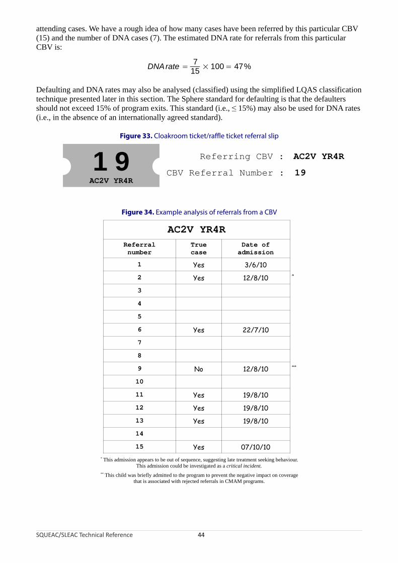
attending cases. We have a rough idea of how many cases have been referred by this particular CBV (15) and the number of DNA cases (7). The estimated DNA rate for referrals from this particular CBV is:
7DNArate = × 100= 47%
15
Defaulting and DNA rates may also be analysed (classified) using the simplified LQAS classification technique presented later in this section. The Sphere standard for defaulting is that the defaulters should not exceed 15% of program exits. This standard (i.e., ≤ 15%) may also be used for DNA rates (i.e., in the absence of an internationally agreed standard).
Figure 33. Cloakroom ticket/raffle ticket referral slip
SQUEAC/SLEAC Technical Reference 44
1 9AC2V YR4R
Referring CBV :
CBV Referral Number :
AC2V YR4R
19
Figure 34. Example analysis of referrals from a CBV
AC2V YR4R
Referralnumber
Truecase
Date ofadmission
1 Yes 3/6/10
2 Yes 12/8/10 *
3
4
5
6 Yes 22/7/10
7
8
9 No 12/8/10 **
10
11 Yes 19/8/10
12 Yes 19/8/10
13 Yes 19/8/10
14
15 Yes 07/10/10* This admission appears to be out of sequence, suggesting late treatment seeking behaviour.
This admission could be investigated as a critical incident.** This child was briefly admitted to the program to prevent the negative impact on coverage
that is associated with rejected referrals in CMAM programs.
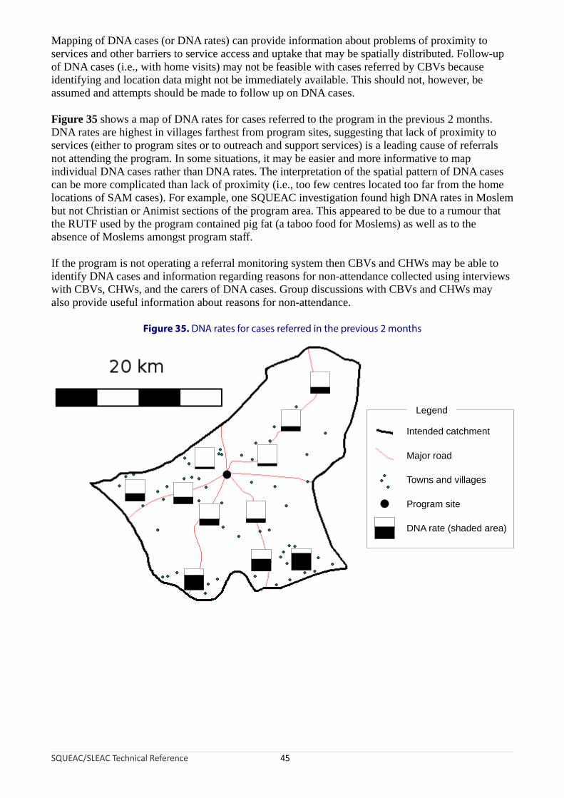
Mapping of DNA cases (or DNA rates) can provide information about problems of proximity to services and other barriers to service access and uptake that may be spatially distributed. Follow-up of DNA cases (i.e., with home visits) may not be feasible with cases referred by CBVs because identifying and location data might not be immediately available. This should not, however, be assumed and attempts should be made to follow up on DNA cases.
Figure 35 shows a map of DNA rates for cases referred to the program in the previous 2 months. DNA rates are highest in villages farthest from program sites, suggesting that lack of proximity to services (either to program sites or to outreach and support services) is a leading cause of referrals not attending the program. In some situations, it may be easier and more informative to map individual DNA cases rather than DNA rates. The interpretation of the spatial pattern of DNA cases can be more complicated than lack of proximity (i.e., too few centres located too far from the home locations of SAM cases). For example, one SQUEAC investigation found high DNA rates in Moslem but not Christian or Animist sections of the program area. This appeared to be due to a rumour that the RUTF used by the program contained pig fat (a taboo food for Moslems) as well as to the absence of Moslems amongst program staff.
If the program is not operating a referral monitoring system then CBVs and CHWs may be able to identify DNA cases and information regarding reasons for non-attendance collected using interviews with CBVs, CHWs, and the carers of DNA cases. Group discussions with CBVs and CHWs may also provide useful information about reasons for non-attendance.
Figure 35. DNA rates for cases referred in the previous 2 months
SQUEAC/SLEAC Technical Reference 45
Intended catchment
Major road
Towns and villages
Program site
Legend
DNA rate (shaded area)
Information Provided by Routine Program Data
Routine program data and readily available contextual data can provide useful information about program coverage:
• Examination of the pattern of admissions over time, admission MUAC, and the need for inpatient facilities can identify potential problems with recruitment procedures.
• Examination of the pattern of defaulters and DNA cases over time can identify potential problems with attendance costs, beneficiary retention, proximity to services, and contact frequency.
• Mapping of beneficiary home locations and outreach activities can identify potential problems with the spatial reach of a program. Simple listing and plotting techniques can identify potential problems with the spatial and temporal coverage of a program.
• Mapping of the home locations of defaulting and DNA cases can identify potential problems with proximity to services and other barriers to service access and uptake that may be spatially distributed. Simple listing and plotting techniques can be used to estimate or classify defaulting and DNA rates.
Routine program data can provide a great deal of useful information about program coverage but it is important to realise that the information provided is limited. Routine program data can identify whether distance is a factor influencing program attendance. Routine program data cannot identify, for example, rude and insulting behaviour toward unmarried mothers by program staff as a leading cause of defaulting and DNA cases. Investigation of these sorts of barriers to access and uptake requires different data collected using different approaches. For example, follow-up visits to defaulting and DNA cases identified from simple analyses of routine program data may be used to identify barriers to service access and uptake.
Data Sources and Methods of Analysis: Qualitative DataThree methods of collecting qualitative data from a variety of sources are commonly used in SQUEAC investigations. These are:
1. Semi-structured interviews with key informants such as:
• Program staff• Clinic staff• Community-based informants such as schoolteachers, traditional healers,
traditional birth attendants (TBAs), health extension workers, agriculture extension workers, and CBVs
• Carers of children in the program• Carers of non-covered, defaulting, and DNA cases
2. Simple structured interviews, undertaken as part of routine program monitoring and during small-area surveys, with:
• Carers of defaulting and DNA cases• Carers of non-covered cases found by surveys
3. Informal group discussions with:
• Carers of children attending program sites• Relatively homogenous groups of key informants (e.g., community leaders and
religious leaders) and lay informants (e.g., mothers and fathers)• Program staff• CBVs
SQUEAC/SLEAC Technical Reference 46

Other methods of collecting qualitative data (e.g., formal focus groups and more structured and in-depth interviews) may also prove useful in some contexts.
The collection of qualitative data should concentrate on discovering reasons for both non-attendance and defaulting.
Methods of Collecting Qualitative Data: Semi-Structured Interviews
Semi-structured interviews are based on an interview guide. This is a set of clear instructions comprising a list of questions that should be asked and topics that should be covered in the interview. Box 1, for example, shows an interview guide for use early in a SQUEAC investigation with carers of children in the program.
The exact order and wording of questions may differ from informant to informant and is likely to change as data collection proceeds and the focus of the data-collection effort changes. The interviewer does not have to stick strictly to the questions in the interview guide and may follow ‘leads’ and new topics as they arise in the course of an interview, although all questions and topics outlined in the interview guide should be covered in each interview.
The use of an interview guide helps the interviewer make efficient use of the time available for an interview. This is important when interviewing informants that may not be able or willing to spend a lot of time in an open-ended discussion with the interviewer.
The structure imposed on the interview by the interview guide shows the informant that you are clear about what you want from the interview. This is important when dealing with, for example, clinic staff and government officials.
The flexibility of being able to investigate new ‘leads’ introduced by the informant sets this method apart from simple structured interviews (see below).
Two types of semi-structured interview have proved useful in SQUEAC investigations:
Focussed interviews (in-depth interviews). Focussed interviews are used to intensively investigate a single topic. The purpose of a focused interview is to gain a complete and detailed understanding of the topic under investigation. Focussed interviews are very useful toward the end of the data-collection effort to resolve discrepancies in previously collected data or when collecting data from informants with an in-depth knowledge about a single topic (e.g., asking outreach workers, CHWs, and CBVs about probable reasons for non-attendance and defaulting). Case histories (case studies). A case history is similar to history-taking in clinical medicine, except that the emphasis of the history is less on eliciting a history of symptoms (although this is useful for identifying mismatches between program and community aetiologies/definitions of malnutrition as in Box 1) and more on eliciting the context to a specific situation. Case histories are most useful when you need to understand a situation in depth and when information-rich cases (e.g., carers of defaulting and DNA cases) can be found.
SQUEAC/SLEAC Technical Reference 47

Box 1. Example interview guide for first interviews with carers of children in a program
How did this child get to be in this program?
The intention of this question is to:
Elicit a history.
Explore local SAM aetiologies.
Explore treatment seeking behaviour/pathways to care (i.e., for contrast with the program’s case-finding and referral methods).
The carer may start by, for example, describing events around case-finding and referral. Keep this as a ‘reference point’ during the interview and probe:
‘What happened after that?’
‘What happened before that?’
Do you know of any children in your village that are like your child that are not attending this program?
When asking and following up on this question, refer to/ask about:
The index child’s specific history (from above).
Common SAM aetiologies (e.g., not recovered well after an illness).
Specific signs (e.g., thin arms, swollen feet, kwashiorkor signs).
Treatment seeking behaviour/pathways to care.
Encourage narratives/histories.
If YES: Why do you think the child is not attending this program?
Reflect back responses to elicit further information.
Probe: ‘How do you know this?’, ‘Any other reasons?’, ‘Any other children?’.
Encourage narratives/histories.
Record the name and home location of the informant for follow-up.
If NO: If there were children like your child that are not attending this program, why do you think they would not attend the program?
Note the question is hypothetical. This may need explaining.
Reflect back responses to elicit further information.
Probe: ‘Any other reasons?’
If I wanted to find children like your child and the children we have spoken about, how would I best describe them to other people?
The intention of this question is to discover local terms and aetiologies for SAM. Probe for definitions of local terms. Some terms will be descriptive. Other terms will reflect local/folk aetiologies (e.g., kwashiorkor is a Ga language term for ‘the sickness the baby gets when the new baby comes’). You will find this useful for case-finding in surveys and to contrast with program messages.
Give examples of specific signs and ask for local terms.
Probe: ‘Any other names for this?’, ‘Will most people understand what I am asking if I ask about [TERM]?’.
Ask about how this differs from the program messages (e.g., ‘Are these [TERMS] the same thing as “malnutrition”?’).
If I wanted to find children like your child and the children we have spoken about, who would best be able to help me to find them?
Probe: ‘Anyone else?’. Make sure you ask directly about midwives/traditional birth attendants, traditional healers, the people mentioned in histories when exploring treatment seeking behaviour/pathways to care (above), and the people used by the program for case-finding and referral.
Probe: ‘Why?’ and ‘Why not?’.
Confirm: ‘You are saying that I should ask [PERSON] to take me to see children with [TERMS]. Is that right?’
This information will be used for case-finding in surveys.
SQUEAC/SLEAC Technical Reference 48

Box 2. Simple structured interview questionnaire to be applied to carers of non-covered cases
Questionnaire for carers of cases not in the program
Village: __________________________________________________________
Program site: __________________________________________________________
Name: __________________________________________________________
__ 1. Do you think that this child is malnourished? |__|
If YES ...
2. Do you know of a program that can treat malnourished children?
__ |__| If YES ...
3. What is the name of this program?
___________________________________________________
4. Where is this program?
___________________________________________________
5. Why is this child not attending this program?
Do not prompt. Probe ‘Any other reason?’ __ |__| Program site is too far away |__| No time/too busy to attend the program |__| Carer cannot travel with more than one child |__| Carer is ashamed to attend the program |__| Difficulty with childcare |__| The child has been rejected by the program
Record any other reasons ...
__________________________________________________
__________________________________________________
__________________________________________________
6. Has this child ever been to the program site or examined by program staff? __ |__| If YES ...
7. Why is this child not in the program now? __ |__| Previously rejected |__| Defaulted |__| Discharged as cured |__| Discharged as not cured
Thank carer. Issue a referral slip. Inform carer of site and date to attend.
The tick box items for question 5 were selected after analysis of the collected program and qualitative data. Using tick boxes forthe most commonly expected responses simplifies both data collection and analysis. See Figure 2 and Figure 45 for
examples of how this type of data should be presented.
SQUEAC/SLEAC Technical Reference 49

Methods of Collecting Qualitative Data: Simple Structured Interviews
Structured interviews expose every informant to the same stimulus. This usually means that the same questions are asked in the same order. Survey questionnaires are an example of a simple structured interview and are used in both SQUEAC assessments and CSAS surveys. Box 2 (previous page) shows an example of a simple structured interview questionnaire that may be applied to carers of non-covered cases found during SQUEAC small-area surveys. A similar questionnaire could be applied to carers of defaulting and DNA cases. The questionnaire shown in Box 2 yields qualitative data (i.e., questions regarding the how? and why? of decision making in carers of non-covered cases) that can be analysed using simple quantitative techniques as in Figure 2 and Figure 45. It should be noted that the use of the case-history approach (see above) may yield important data from carers of defaulting and DNA cases that cannot be captured by a simple structured interview.
Methods of Collecting Qualitative Data: Informal Group Discussions
With informal group discussions, the interviewer has an idea of the topics that are to be covered in the interview, but there is no strict order in which the topics are to be covered and there is no strict wording of the questions to be asked. The discussion should be informal and conversational. Informants are encouraged to express themselves in their own terms rather than those dictated by the interviewer.
The key skill for the leader of a successful informal group discussion is the ability to stimulate informants to provide useful data without injecting too many of the interviewer’s words and concepts into the discussion. The group discussion approach allows the interviewer to respond to differences between informants and to follow and explore ‘leads’ as they arise.
The basic focus of informal group discussions in SQUEAC investigations is to discover reasons for non-attendance and defaulting. The informants usually either will not have a child eligible for entry into the program (e.g., community leaders) or will already have a child attending the program (e.g., carers of children attending program sites). This means that the collected data are often limited to perceptions of the motivations of others, rather than direct reports of personal motives. Data collected using informal group discussions in these groups are, therefore, most useful for finding relevant questions and wordings for later semi-structured and structured interviews with other informants and should always be triangulated with data collected using other methods.
Informal group discussions can be useful sources of information about perceptions of health services and consumer experiences with health services. It is particularly important to collect this data when investigating the coverage of integrated CMAM services (e.g., CMAM services delivered using government-run health facilities as part of an integrated management of childhood illness [IMCI] package). In this context, informants may not be able to distinguish between CMAM services and general healthcare provision, and negative opinions and negative experiences of clinics might act to reduce the coverage of all services, including CMAM services.
Validating and Analysing Qualitative Data
It is important that the collected qualitative data are validated. In practice, this means that data are collected from as many different sources as possible. Data sources are then cross-checked against each other. If data from one source are confirmed by data from another source then the data can be considered to be useful. If data from one source is not confirmed by data from other sources then more data should be collected, either from the same sources or from new sources, for confirmation. This process is known as triangulation.
SQUEAC/SLEAC Technical Reference 50

There are two types of triangulation:
• Triangulation by source refers to data confirmed by more than one source. It is better to have data confirmed by more than one type of source (e.g., community leaders and clinic staff) rather than just by more than one of the same type of source. Type of source may also be defined by demographic, socio-economic, and spatial attributes of informants. Lay informants such as mothers and fathers are sources of differing gender. Lay informants from different economic strata, different ethnic groups, different religious groups, or widely separated locations are also different types of source.
• Triangulation by method refers to data confirmed by more than one method. It is better to have data confirmed by more than one method (e.g., semi-structured interviews and informal group discussions) than by a single method.
You should plan data collection to ensure triangulation by both source and method. Table 3, for example, shows an example data collection plan for triangulation regarding seasonal calendars.
Table 3. A data collection plan for triangulation by source and method of data regarding seasonal calendars of disease, labour demand, and food availability
Data Source Method Person Notes
Diseasecalendar
Medical assistant SSI Farah
Nursing staff SSI Farah
Carers IDI Sara Add to histories
Carers IGD Iptihalat
Clinic returns Data extraction FarahClinic and state Ministry of
Health
TBA SSI Iptihalat
Traditional healer SSI Farah
Labourcalendar
Tea-shop customers IGD Taj El Dein
Carers IGD Iptihalat
Clinic guard SSI Farah
Agriculture extension worker
SSI Taj El Dein
Foodavailability
calendar
Tea-shop customers IGD Taj El Dein
Agricultureextension worker
SSI Taj El Dein
Carers IGD Iptihalat
Market dataData
extractionFarah WFP monitoring data
SSI = Semi-structured interview; IDI = In-depth (focussed) interview; IGD = Informal group discussion
Data courtesy UNICEF Sudan
SQUEAC/SLEAC Technical Reference 51

Data from qualitative sources and methods are also triangulated with routine program data and data from small studies, small surveys, and small-area surveys (Figure 36).
Figure 36. Triangulation of SQUEAC data
SQUEAC/SLEAC Technical Reference 52
Routineprogram data
Small-areasurveys
Informalgroup
discussions
Semi-structuredinterviews
Structuredinterviews
Reasons fornon-attendanceand defaulting
Spatial patternof coverage
Small surveys
Small studies

Data collection using triangulation is a purposeful and intelligent process. Data from different sources and methods should be regularly and frequently compared with each other. Discrepancies in the data are then used to inform decisions about whether to collect further data. If further data collection is required, these discrepancies help determine which data to collect, as well as the sources and methods to be used.
It is important that the data are exhaustive. This means identifying as many useful data sources as possible and continuing to collect data until no new information is coming to light. This process is known as sampling to redundancy.
Collection, validation, and analysis of qualitative data are not separate processes. Data are analysed during collection and more data are collected to confirm or deny findings using both triangulation and sampling to redundancy.
Storing, Organising, and Analysing Findings
The semi-quantitative approach used in SQUEAC investigations collects a broad set of data using a variety of methods from diverse sources in an intelligent and purposive manner. This is very different from the traditional survey approach in which a narrow set of data is collected using a single method (e.g., structured interview by formal questionnaire) from a large number of the same type of data source in a mechanistic manner.
Both the SQUEAC and traditional survey approaches need tools to store and organise findings. The survey approach uses tools such as spreadsheets and databases. These tools are well suited to working with survey data. Data are entered and stored as rows in a spreadsheet or as records in a database. Data analysis is usually performed only when all data has been collected, entered, checked, and cleaned. Data collection, validation (checking), and analysis are separate processes that follow each other in time.
Spreadsheets and databases are useful in SQUEAC investigations for working with data from purely quantitative sources, such as standard program indicators, admission over time, MUAC at admission, and time-to-travel. SQUEAC data are simple enough to be collected and analysed using paper databases and spreadsheets (e.g., Figure 23; Table 1, page 31; and Figure 34) and tally sheets (e.g., Figure 14, Figure 27, and Figure 44). SQUEAC treats this sort of data just like survey data, with data being collected, entered, checked, and then analysed numerically or graphically. These are, however, just components of a much broader SQUEAC dataset collected using the principles of triangulation (by source and method) and sampling to redundancy.
Spreadsheets and databases are not very useful when dealing with data collected using the principles of triangulation (by source and method) and sampling to redundancy. This is because:
• The data are in a variety of formats ranging from, for example, a simple column of numbers representing admission MUACs to a detailed discussion of local/folk aetiologies and traditional treatment of SAM with a traditional healer. Each type of data is organised, stored, analysed, and presented in different ways. Spreadsheets and databases work best when all data are organised, stored, analysed, and presented in the same way.
• Data are analysed as they are collected. Data from different sources and methods are compared with each other. Discrepancies in the data are then used to inform decisions about whether to collect further data. If further data collection is required, these discrepancies help determine which data to collect, as well as the sources and methods to be used. Spreadsheets and databases work best when data analysis is performed after all data have been collected.
SQUEAC/SLEAC Technical Reference 53

What is required is a means of storing, organising, and analysing data that is designed to generate, visualise, structure, and classify data and ideas in order to solve problems, make decisions, and aid in summarising and reporting complex data. SQUEAC uses techniques known as concept-mapping and mind-mapping to do this:
• Concept-mapping is a graphical data-analysis technique that is useful for representing relationships between findings. Concept-maps show findings and the connections (relationships) between findings. Figure 13 is an example of a concept-map using only ‘results in’ or ‘leads to’ relationships. Other types of relationships (e.g., ‘required for’, ‘contributes to’, ‘encourages’, ‘helps create’, ‘allows’) may be specified (as in Figure 37) and explanatory annotations added (as in Figure 38). Concept-maps are useful for note-taking during interviews, when working out and communicating how different findings (e.g., barriers) are related and interact with each other each other in complex or cyclical processes (e.g., vicious or virtuous circles), and in forming hypotheses for further investigation. Concept-maps are also useful when scoring findings to estimate overall program coverage.
• Mind-mapping is a graphical way of storing and organising data and ideas. A mind-map organises findings using tree structures organised around a central theme and summarises the findings of a SQUEAC investigation. It is drawn and modified as the investigation proceeds. Figure 39 shows an example of a mind-map from a SQUEAC investigation.
A mind-map is used to summarise the findings of the SQUEAC investigation and is drawn and modified as the investigation proceeds. Figure 40 shows a mind-map as it developed during a SQUEAC investigation.
Mind-maps may be created using some (or all) of the following guidelines:
• Start with the central theme (‘Coverage’) in the centre of the page.
• Keep the mind-map clear by using a branching hierarchy. SQUEAC mind-maps tend to use the hierarchy of:
Central Theme → Data Source/Method → Individual Findings
• Present each finding alone; relationships between findings may be shown using, for example, dotted lines, symbols, or colours.
• Use images, symbols, and codes throughout the mind-map:
• Use the ? symbol to mark unconfirmed findings.
• Use the ✓ or ↑ symbol to mark positive findings.
• Use the ✗ or ↓ symbol to mark negative findings.
• Use the ~ or ↔ symbol to mark neutral findings.
• Combine symbols (e.g., use ?↑ to mark unconfirmed but indicative positive findings).
• Use boxes, circles, shading, etc. for emphasis.
• Write key words using uppercase or lowercase letters and use colour and underlining.
• Lines should be connected and start from the central theme.
• Vary line thickness to denote importance/influence.
• Use colours throughout the mind-map to encode or group.
• Use emphasis and show relationships in the mind-map.
• Redraw and re-organise the mind-map as it becomes confused and untidy.
These are guidelines, not rules. The only rule is that findings should be organised in tree structures organised around a central theme.
SQUEAC/SLEAC Technical Reference 54

Figure 37. An example of a concept-map using explicitly defined relationship types
Data courtesy of Save the Children (USA) and the Friedman School of Nutrition Science and Policy (Tufts University)
Note: This concept-map shows an example of a virtuous cycle driving coverage up and keeping coverage high.
SQUEAC/SLEAC Technical Reference 55
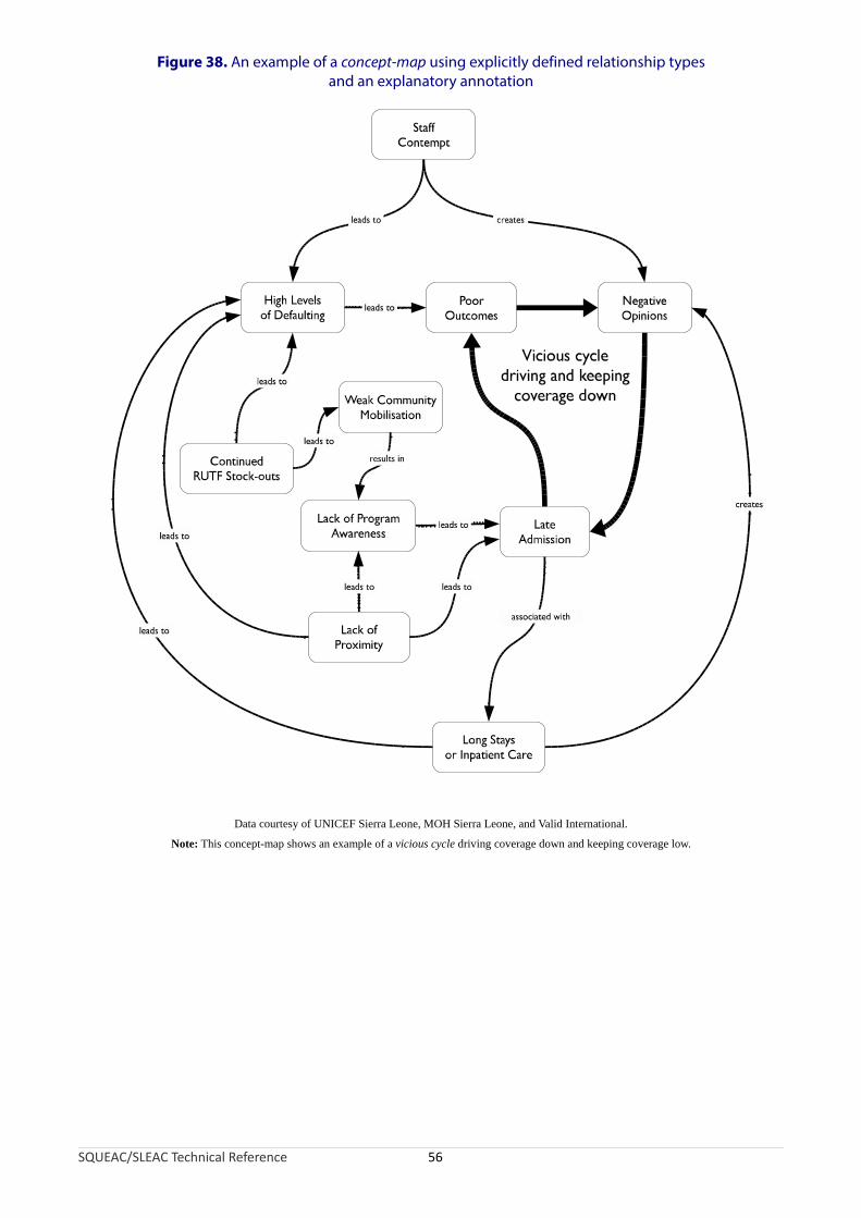
Figure 38. An example of a concept-map using explicitly defined relationship types and an explanatory annotation
Data courtesy of UNICEF Sierra Leone, MOH Sierra Leone, and Valid International.
Note: This concept-map shows an example of a vicious cycle driving coverage down and keeping coverage low.
SQUEAC/SLEAC Technical Reference 56
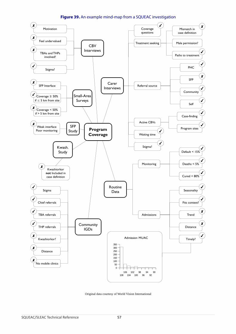
Figure 39. An example mind-map from a SQUEAC investigation
Original data courtesy of World Vision International
Coverage < 50%if > 5 km from site
CarerInterviews
Coveragequestions
Mismatch incase definition
Male permission?
Paths to treatment
Referral source
Active CBVs
Waiting time
Case-finding
Program sites
Stigma?
PHC
SFP
Community
Self
RoutineData
Monitoring
Default < 15%
Deaths < 5%
Cured < 80%
Admissions
Seasonality
Fits context?
Trend
Distance
Timely?
CBVInterviews
Motivation
Feel undervalued
TBAs and THPsinvolved?
Stigma?
CommunityIGDs
Stigma
Chief referrals
TBA referrals
THP referrals
Kwashiorkor?
Distance
No mobile clinics
Kwash.Study
Kwashiorkornot Included incase definition
SFPStudy
Weak interfacePoor monitoring
Small-AreaSurveys
SFP Interface
Coverage ≥ 50%if ≤ 5 km from site
ProgramCoverage
✘
✘
✘
✘
✘
✘
✘
✘
✘
✘
✔
✔
✔
✔
✔
✔
✘
✘
✘
✘
✔
✔
✔
✔
✔
✔
✔
✔
✔
✔
✔
✔
✔
✔
✔
108106
104102
10098
9694
9290
0
50
100
150
200
250
300
350
Admission MUAC
Treatment seeking
SQUEAC/SLEAC Technical Reference 57
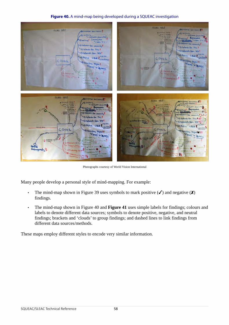
Figure 40. A mind-map being developed during a SQUEAC investigation
Photographs courtesy of World Vision International
Many people develop a personal style of mind-mapping. For example:
• The mind-map shown in Figure 39 uses symbols to mark positive (✓) and negative (✗) findings.
• The mind-map shown in Figure 40 and Figure 41 uses simple labels for findings; colours and labels to denote different data sources; symbols to denote positive, negative, and neutral findings; brackets and ‘clouds’ to group findings; and dashed lines to link findings from different data sources/methods.
These maps employ different styles to encode very similar information.
SQUEAC/SLEAC Technical Reference 58

Figure 41. A completed SQUEAC mind-map (following from Figure 40)
Photograph courtesy of World Vision International
The style of mind-mapping extends to the organisation or branching hierarchy of the tree structure around the central theme. Trees may be organised using source → method → issue as branching hierarchy:
SQUEAC/SLEAC Technical Reference 59
CentralTheme
Source
IssueMethod
Method
Method
Issue
Method
Findings
FindingsSource
Issue
Method Method
Issue
Method
Findings Findings
Source
Issue
Method
Method
MethodIssue
Method
Findings
Findings
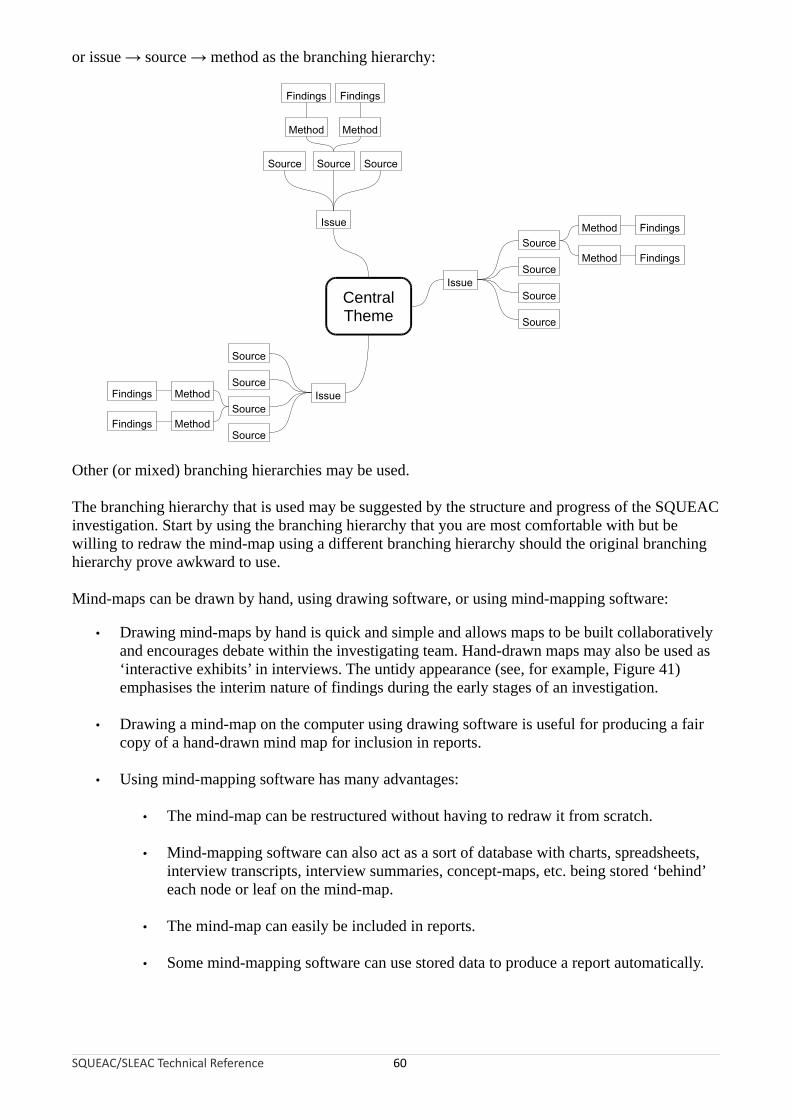
or issue → source → method as the branching hierarchy:
SQUEAC/SLEAC Technical Reference 60
CentralTheme
Issue
MethodSource
Source
Source
Method
Source
Findings
Findings
Issue
Method
Source Source
Method
Source
Findings Findings
Issue
Method
Source
Source
SourceMethod
Source
Findings
Findings
Other (or mixed) branching hierarchies may be used.
The branching hierarchy that is used may be suggested by the structure and progress of the SQUEAC investigation. Start by using the branching hierarchy that you are most comfortable with but be willing to redraw the mind-map using a different branching hierarchy should the original branching hierarchy prove awkward to use.
Mind-maps can be drawn by hand, using drawing software, or using mind-mapping software:
• Drawing mind-maps by hand is quick and simple and allows maps to be built collaboratively and encourages debate within the investigating team. Hand-drawn maps may also be used as ‘interactive exhibits’ in interviews. The untidy appearance (see, for example, Figure 41) emphasises the interim nature of findings during the early stages of an investigation.
• Drawing a mind-map on the computer using drawing software is useful for producing a fair copy of a hand-drawn mind map for inclusion in reports.
• Using mind-mapping software has many advantages:
• The mind-map can be restructured without having to redraw it from scratch.
• Mind-mapping software can also act as a sort of database with charts, spreadsheets, interview transcripts, interview summaries, concept-maps, etc. being stored ‘behind’ each node or leaf on the mind-map.
• The mind-map can easily be included in reports.
• Some mind-mapping software can use stored data to produce a report automatically.

Figure 42 shows a SQUEAC mind-map being edited using an open-source mind-mapping software package called XMind. This is available free from:
http://www.xmind.net/
This screenshot shows the text stored ‘behind’ the node for the findings of interviews with village doctors as well as a graph of routine program monitoring data. The XMind software can automatically produce a formatted and illustrated report using the entered findings and the hierarchical structure of the mind-map.
Most SQUEAC investigators use both hand-drawn mind-maps and mind-mapping software. It is particularly useful to use both methods during training. A large hand-drawn mind-map, such as is shown in Figure 40 and Figure 41, is useful for managing a SQUEAC investigation, providing a rich summary of the current state of the investigation and can serve as a focal point when deciding data-collection needs and dividing tasks between team members. The collaborative focus provided by the mind-map facilitates team building and improves the quality of the investigation.
SQUEAC/SLEAC Technical Reference 61
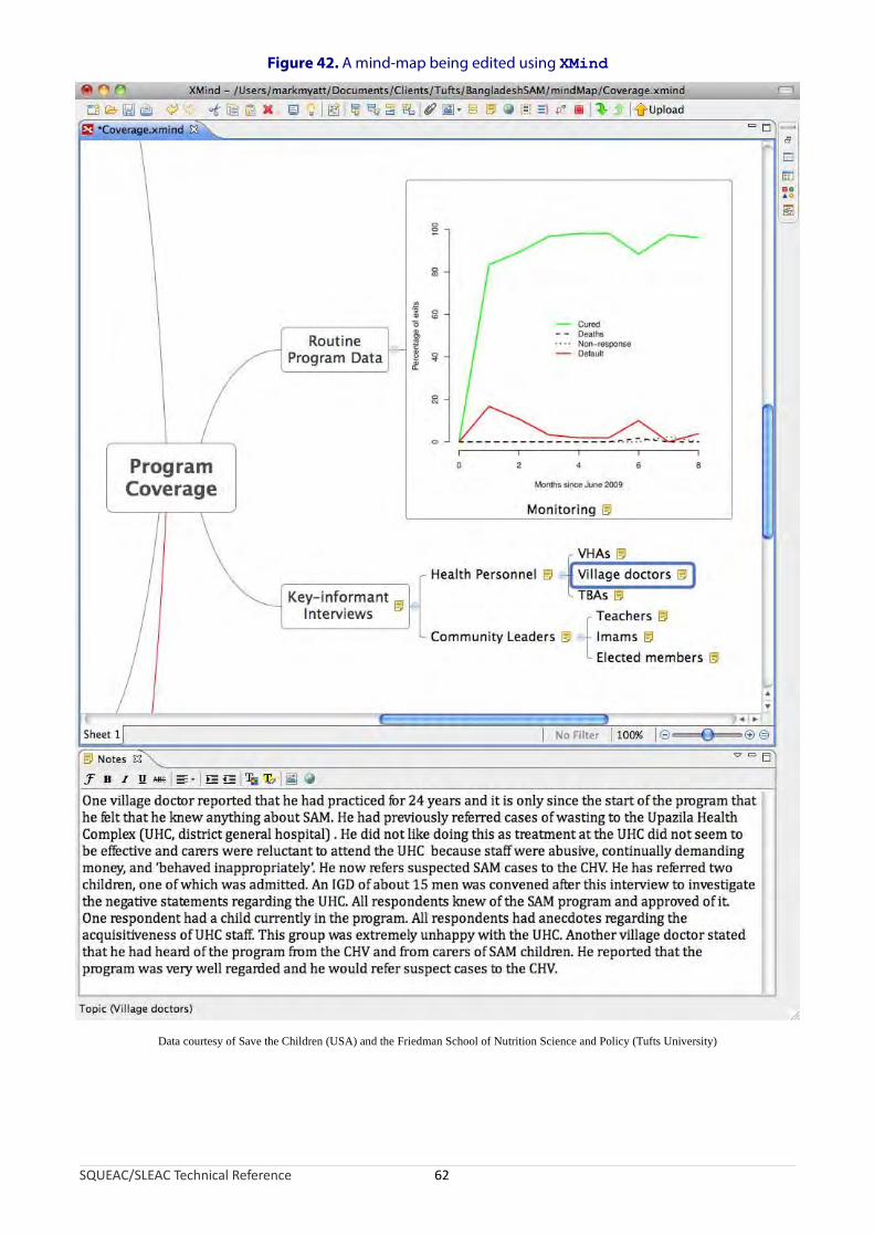
Figure 42. A mind-map being edited using XMind
Data courtesy of Save the Children (USA) and the Friedman School of Nutrition Science and Policy (Tufts University)
SQUEAC/SLEAC Technical Reference 62
Combining and Confirming Findings from Routine Program and Qualitative Data
The data collected from routine program data and qualitative data, when combined, provide information about where coverage is likely to be satisfactory and where coverage is likely to be unsatisfactory, as well as information about the likely barriers to service access and uptake that exist within a program (Figure 36). This information can be considered or stated as a set of hypotheses that can be tested. The SQUEAC method uses small studies, small surveys, and small-area surveys to test these hypotheses.
Organising findings using concept-maps and mind-maps helps in formulating hypotheses. The findings shown in the mind-map in Figure 39, for example, suggested (amongst other things) the following hypotheses:
1. There will be a number of cases that were admitted to a supplementary feeding program (SFP) but that failed to respond and have become severely malnourished. This has not been recognised and they are now in the wrong program. These cases are not covered. This hypothesis was suggested by the absence of referrals from the SFP to the therapeutic feeding program (TFP). This hypothesis was tested by a small study at SFP sites, which revealed that there was no effective monitoring system in the SFP (leaving SAM cases undetected) and that SFP staff were unsure how to transfer cases from the SFP to the TFP. Small-area surveys also found SAM cases that were (inappropriately) in the SFP.
2. Distance between program sites and communities is a significant barrier to access. This is suggested by the analysis of admissions, by informal group discussions in outlying communities, and by the request for mobile clinics made in pastoralist communities. This hypothesis was tested using several small-area surveys undertaken in communities at different distances from program sites. These surveys found good coverage in communities located within 5 km of a program site and poor coverage in communities located further than 5 km from a program site.
Hypotheses about coverage should always be stated before undertaking small studies, small surveys, or small-area surveys. Hypotheses about coverage will usually take the form of identifying areas where the combined data suggest that coverage is likely to be satisfactory and areas where the combined data suggest that coverage is likely to be unsatisfactory. Figure 43, for example, shows an area of probable low coverage identified by mapping beneficiary home locations, analysis of outreach activities, defaulter follow-up, and qualitative data. The hypothesis about coverage in this area was:
• Coverage is below the Sphere minimum standard for coverage of TFPs in rural settings of 50% due to:
• A mismatch between the program’s definition of malnutrition (i.e., anthropometric criteria and problems of food-security) and the community’s definition of malnutrition (i.e., as a consequence of illness, particularly diarrhoea with fever).
• Patchy coverage of outreach services, particularly with regard to the ongoing follow-up of children with marginal anthropometric status.
• Distance to program sites and other opportunity costs.
A small-area survey was undertaken in this area to confirm this hypothesis. This survey involved using active and adaptive case-finding (see Box 3, page 65) in all villages in the area identified (shaded) in Figure 43 and the application of a questionnaire similar to that shown in Box 2 (page 49) to carers of non-covered cases found by the survey. Analysis of the collected data confirmed that coverage in the identified area was likely to be below 50%. The data are shown in Figure 44 and the details of the analysis are shown below.
SQUEAC/SLEAC Technical Reference 63

Figure 43. Area of probable low coverage identified by mapping of home locations (shown), analysis of outreach activities, defaulter follow-up, and qualitative data
Photograph courtesy of Concern Worldwide
SQUEAC/SLEAC Technical Reference 64
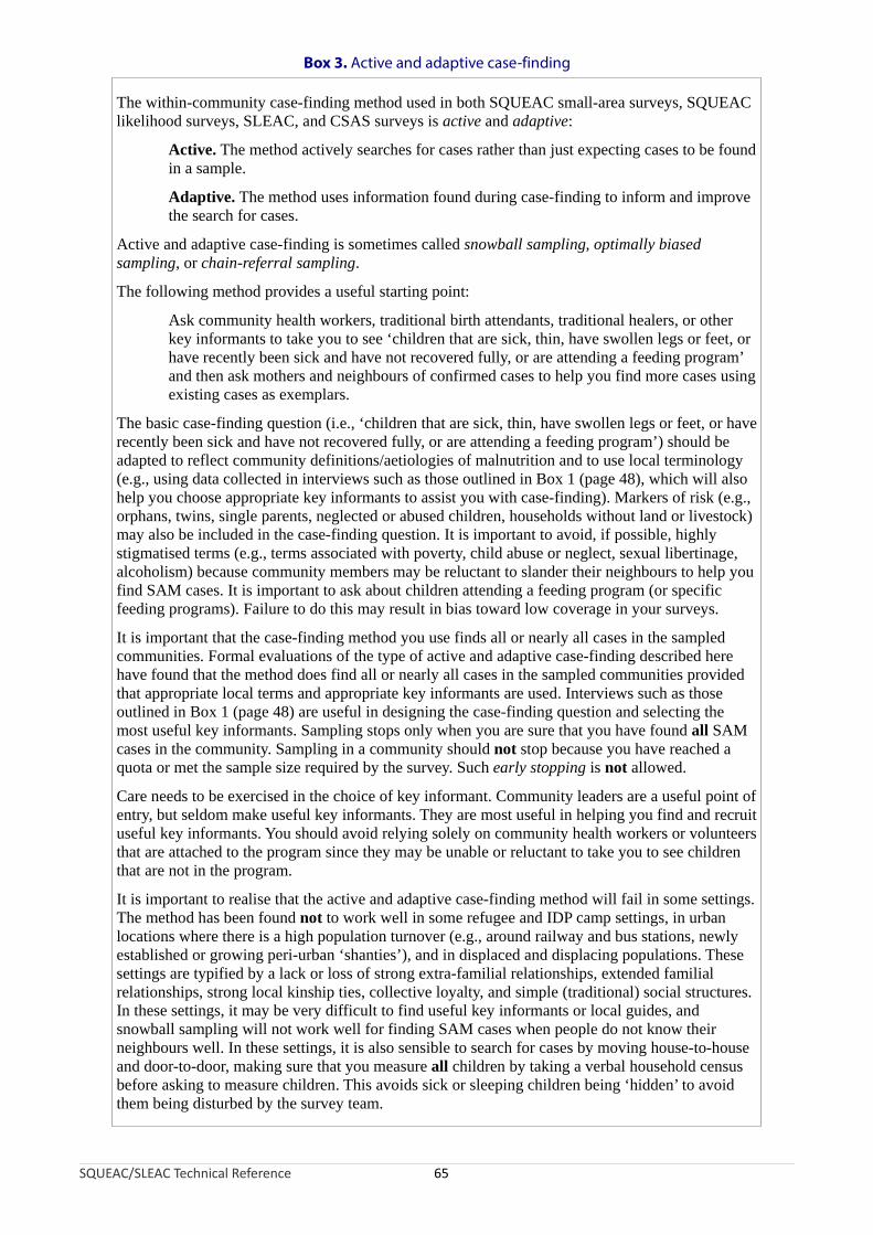
Box 3. Active and adaptive case-finding
The within-community case-finding method used in both SQUEAC small-area surveys, SQUEAC likelihood surveys, SLEAC, and CSAS surveys is active and adaptive:
Active. The method actively searches for cases rather than just expecting cases to be found in a sample.
Adaptive. The method uses information found during case-finding to inform and improve the search for cases.
Active and adaptive case-finding is sometimes called snowball sampling, optimally biased sampling, or chain-referral sampling.
The following method provides a useful starting point:
Ask community health workers, traditional birth attendants, traditional healers, or other key informants to take you to see ‘children that are sick, thin, have swollen legs or feet, or have recently been sick and have not recovered fully, or are attending a feeding program’ and then ask mothers and neighbours of confirmed cases to help you find more cases using existing cases as exemplars.
The basic case-finding question (i.e., ‘children that are sick, thin, have swollen legs or feet, or have recently been sick and have not recovered fully, or are attending a feeding program’) should be adapted to reflect community definitions/aetiologies of malnutrition and to use local terminology (e.g., using data collected in interviews such as those outlined in Box 1 (page 48), which will also help you choose appropriate key informants to assist you with case-finding). Markers of risk (e.g., orphans, twins, single parents, neglected or abused children, households without land or livestock) may also be included in the case-finding question. It is important to avoid, if possible, highly stigmatised terms (e.g., terms associated with poverty, child abuse or neglect, sexual libertinage, alcoholism) because community members may be reluctant to slander their neighbours to help you find SAM cases. It is important to ask about children attending a feeding program (or specific feeding programs). Failure to do this may result in bias toward low coverage in your surveys.
It is important that the case-finding method you use finds all or nearly all cases in the sampled communities. Formal evaluations of the type of active and adaptive case-finding described here have found that the method does find all or nearly all cases in the sampled communities provided that appropriate local terms and appropriate key informants are used. Interviews such as those outlined in Box 1 (page 48) are useful in designing the case-finding question and selecting the most useful key informants. Sampling stops only when you are sure that you have found all SAM cases in the community. Sampling in a community should not stop because you have reached a quota or met the sample size required by the survey. Such early stopping is not allowed.
Care needs to be exercised in the choice of key informant. Community leaders are a useful point of entry, but seldom make useful key informants. They are most useful in helping you find and recruit useful key informants. You should avoid relying solely on community health workers or volunteers that are attached to the program since they may be unable or reluctant to take you to see children that are not in the program.
It is important to realise that the active and adaptive case-finding method will fail in some settings. The method has been found not to work well in some refugee and IDP camp settings, in urban locations where there is a high population turnover (e.g., around railway and bus stations, newly established or growing peri-urban ‘shanties’), and in displaced and displacing populations. These settings are typified by a lack or loss of strong extra-familial relationships, extended familial relationships, strong local kinship ties, collective loyalty, and simple (traditional) social structures. In these settings, it may be very difficult to find useful key informants or local guides, and snowball sampling will not work well for finding SAM cases when people do not know their neighbours well. In these settings, it is also sensible to search for cases by moving house-to-house and door-to-door, making sure that you measure all children by taking a verbal household census before asking to measure children. This avoids sick or sleeping children being ‘hidden’ to avoid them being disturbed by the survey team.
SQUEAC/SLEAC Technical Reference 65
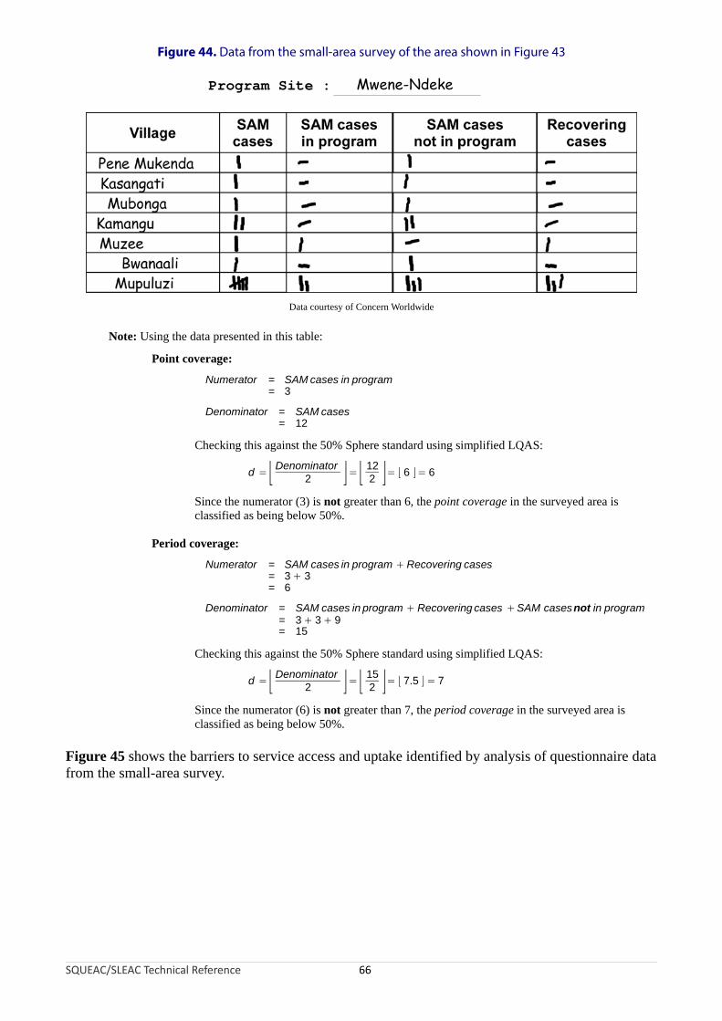
Figure 44. Data from the small-area survey of the area shown in Figure 43
Data courtesy of Concern Worldwide
Program Site : Mwene-Ndeke
Note: Using the data presented in this table:
Point coverage:
Numerator = SAM cases in program= 3
Denominator = SAM cases= 12
Checking this against the 50% Sphere standard using simplified LQAS:
d =⌊ Denominator 12= = ⌊ 6 ⌋= 62 ⌋ ⌊ 2 ⌋
Since the numerator (3) is not greater than 6, the point coverage in the surveyed area is classified as being below 50%.
Period coverage:
Numerator = SAM cases in program + Recovering cases= 3 + 3= 6
Denominator = SAM cases in program + Recovering cases +SAM casesnot in program= 3 + 3 + 9= 15
Checking this against the 50% Sphere standard using simplified LQAS:
d =⌊ Denominator2 ⌋= ⌊ 15
2 ⌋= ⌊ 7.5 ⌋ = 7
Since the numerator (6) is not greater than 7, the period coverage in the surveyed area is classified as being below 50%.
Figure 45 shows the barriers to service access and uptake identified by analysis of questionnaire data from the small-area survey.
SQUEAC/SLEAC Technical Reference 66

Figure 45. Barriers to service uptake found in a SQUEAC small-area survey
Data courtesy of Concern Worldwide
Note: This type of graph is most effective when you have a limited number (e.g., ≤ 10) of barriers to report. Similar barriers should be grouped together. For example, the barriers:
Carer not aware of program
Carer did not know location of program site
Carer did not know that the program site provided RUTF
could be merged into a single ‘Lack of knowledge about the program’ category.
Infrequently reported barriers should be grouped into a single ‘Other’ category. Pie charts should not be used to present this type of data.
The findings of the small-area survey confirmed, in general terms, the hypothesis under test and also identified a problem with the application of case definitions leading to some cases being admitted to the wrong program (i.e., some SAM cases were admitted to the SFP due to confusion around the use of weight-for-height and MUAC in admission criteria).
Information collected regarding barriers to service access and uptake may also be used to inform the design of a questionnaire that is applied to carers of non-covered cases found by small-area surveys. A variation on the standard CSAS questionnaire, such as that shown in Box 2 (page 49), will usually be used for this purpose.
Small-area surveys are used to test hypotheses regarding the spatial distribution of coverage:
• If previously collected data indicates that coverage is likely to be patchy then small-area surveys are used to test this hypothesis. This requires surveys in areas where coverage is believed to be high as well as in areas where coverage is believed to be low.
• If previously collected data indicates that coverage is likely to be even then small-area surveys are used to test this hypothesis. The hypothesis states that coverage will be high (or low) wherever we look. This hypothesis can be tested by selecting survey areas at random. A better approach might be to select survey areas purposively (e.g., at different distances from program sites). A convenience sampling approach should never be used to test this hypothesis, as this is likely to sample areas close to program sites or along roads connecting program sites where coverage is expected to be similar.
Small-area surveys are used in almost all SQUEAC investigations.
SQUEAC/SLEAC Technical Reference 67
Data Sources and Methods of Analysis
SQUEAC uses small studies and surveys to test hypotheses about coverage generated by the analysis of routine program data and qualitative data. Three types of investigation are commonly used:
Small studies. Small studies are usually short, semi-quantitative pieces of work that focus on testing a single hypothesis. The hypothesis being tested usually relates to processes that affects coverage rather than to coverage directly. Sampling and study design are directed by the hypothesis being tested. For example, testing a hypothesis that patient monitoring in an SFP was poor might be investigated by an observational study (i.e., a study in which the SFP processes are observed) at one or more SFP sites. If the hypothesis being tested can be expressed quantitatively (e.g., ‘less than 80% of cases that have been in the program for at least 4 weeks and have failed to gain weight have received counselling from clinic staff’) then data can be analysed using the simplified LQAS classification technique outlined below. Some small studies may be descriptive. In programs with high defaulting rates, for example, a small study finding defaulters and asking about reasons for non-attendance may provide information that can guide program reforms. Figure 46, for example, displays a ranked list of reasons for defaulting found in a rural CMAM program with unacceptably high levels of defaulting.
Small surveys. Small sample surveys are undertaken in population groups that are hypothesised to have high or low coverage (e.g., agrarians and pastoralists, Christians and Moslems). Each and every group is surveyed separately. If population groups live apart and members of each group are relatively easy to identify (e.g., agrarians and pastoralists) then separate small-area surveys (see below) in each population group may be undertaken. If population groups do not live apart then a single survey may be undertaken and data on group membership collected for all cases. The survey dataset may then be divided after data collection and the data from the different groups analysed separately. When using a single survey to collect data on two or more groups, you need to make sure that you use all appropriate local terms in case-finding questions. You may also need to recruit different key informants to help with case-finding in different groups. Data from small surveys may be analysed using the simplified LQAS classification technique outlined below.
Small-area surveys. Small-area surveys are small sample size surveys used to test hypotheses regarding the spatial distribution of coverage. Results may be combined with previously collected data (e.g., time-to-travel plots, carer interviews, half-distance between markets) to draw maps of coverage.
Small surveys and small-area surveys tend to use the same in-community sampling and data-collection methods as CSAS surveys, with communities or sub-communities selected purposively (i.e., directed by the hypothesis being tested). Cases are found using an active and adaptive case-finding method (Box 3, page 65). When a case is found, the carer is asked whether the child is already in the program. A short questionnaire (Box 2, page 49) is administered if the malnourished child is not already in the program.
SQUEAC/SLEAC Technical Reference 68
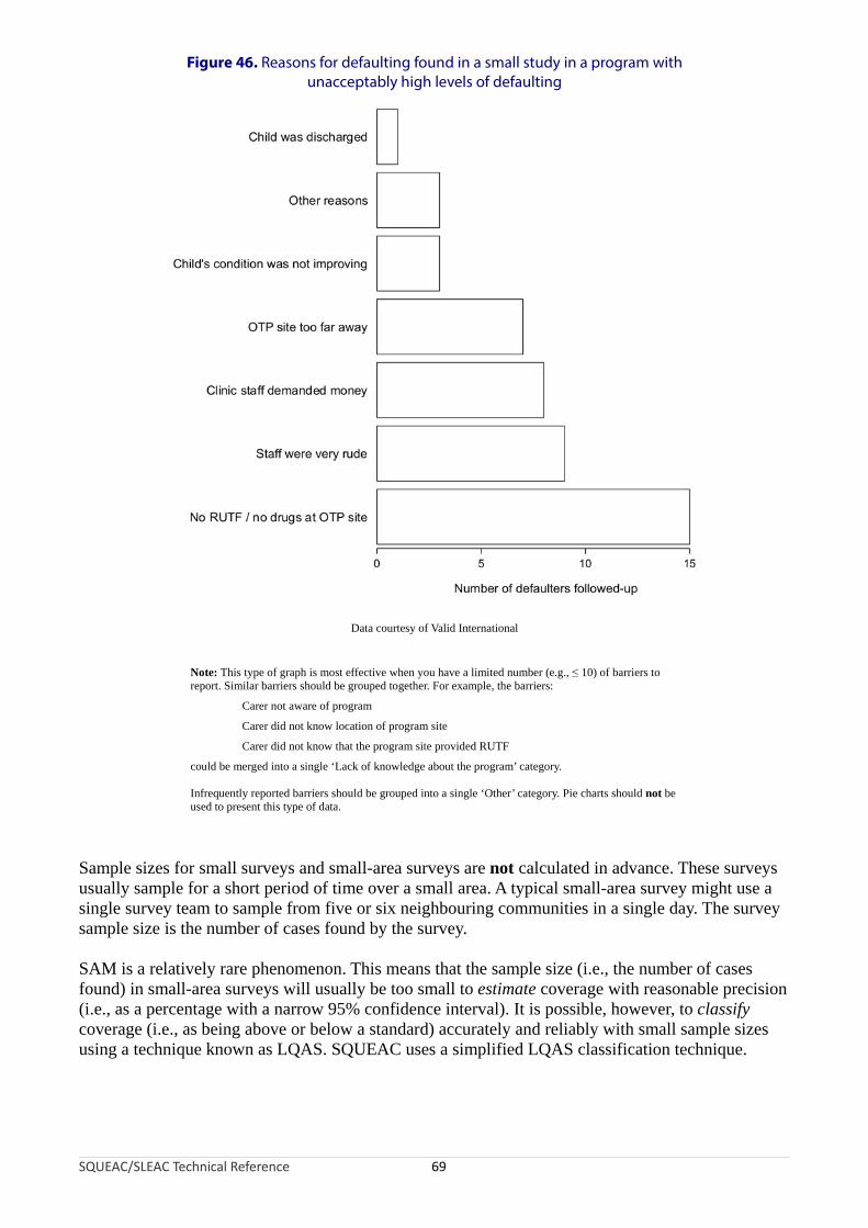
Figure 46. Reasons for defaulting found in a small study in a program with unacceptably high levels of defaulting
Data courtesy of Valid International
Note: This type of graph is most effective when you have a limited number (e.g., ≤ 10) of barriers to report. Similar barriers should be grouped together. For example, the barriers:
Carer not aware of program
Carer did not know location of program site
Carer did not know that the program site provided RUTF
could be merged into a single ‘Lack of knowledge about the program’ category.
Infrequently reported barriers should be grouped into a single ‘Other’ category. Pie charts should not be used to present this type of data.
Sample sizes for small surveys and small-area surveys are not calculated in advance. These surveys usually sample for a short period of time over a small area. A typical small-area survey might use a single survey team to sample from five or six neighbouring communities in a single day. The survey sample size is the number of cases found by the survey.
SAM is a relatively rare phenomenon. This means that the sample size (i.e., the number of cases found) in small-area surveys will usually be too small to estimate coverage with reasonable precision (i.e., as a percentage with a narrow 95% confidence interval). It is possible, however, to classify coverage (i.e., as being above or below a standard) accurately and reliably with small sample sizes using a technique known as LQAS. SQUEAC uses a simplified LQAS classification technique.
SQUEAC/SLEAC Technical Reference 69

Analysis of data using the simplified LQAS classification technique involves examining the number of cases found (n) and the number of covered cases found:
• If the number of covered cases found exceeds a threshold value (d) then coverage is classified as being satisfactory (i.e., coverage meets or exceeds the standard).
• If the number of covered cases found does not exceed this threshold value (d) then coverage is classified as being unsatisfactory (i.e., coverage does not meet or exceed the standard).
The threshold value (d) depends on the number of cases found (n) and the standard (p) against which coverage is being evaluated.
A specific combination of n and d is called a sampling plan.
The Sphere minimum standard for coverage of TFPs in rural settings is 50%. The following rule-of-thumb formula may be used to calculate a value of d appropriate for classifying coverage as being above or below a standard of 50% for any sample size (n):
d = ⌊ n2 ⌋
The ⌊ and ⌋ symbols mean that you should round down the number between the ⌊ and ⌋ symbols to the nearest whole number. For example:
⌊ 6.5 ⌋ = 6
With a sample size (n) of 11, for example, an appropriate value for d would be:
⌊ n ⌋ ⌊ 11d = =
2 2 ⌋= ⌊ 5.5 ⌋ = 5
For standards other than 50%, the following rule-of-thumb formula may be used to calculate a suitable threshold value (d) for any coverage proportion (p) and any sample size (n):
d = ⌊ pn ×
100 ⌋For example, with a sample size (n) of 11 and a coverage proportion (p) of 70% (i.e., the Sphere minimum standard for coverage of TFPs in urban and camp settings), an appropriate value for d would be:
d = ⌊ pn ×
100 ⌋= ⌊ 7011 ×
100 ⌋= ⌊ 11 × 0.7 ⌋ = ⌊ 7.7 ⌋ = 7
The sample size (n) is seldom decided in advance of collecting data but is the number of current SAM cases (or current and recovering SAM cases) found by a survey. This is usually limited to the number of cases that can be found by a single survey team in a single day. The appropriate value for d is calculated after the survey data have been collected.
Figure 47 shows a nomogram that can be used to find appropriate values for d given n and p.
SQUEAC/SLEAC Technical Reference 70

Figure 47. Simplified LQAS nomogram for finding d given n and p
SQUEAC/SLEAC Technical Reference 71
0 5 10 15 20 25 30 35 40 450
10
20
30
40
50
d (round down to nearest whole number)
Sam
ple
size
(n
)p = 10% p = 20% p = 30% p = 40% p = 50% p = 60% p = 70% p = 80% p = 90%
Example showing d = 15 when n = 22 and p = 70%

Figure 44 shows the data collected in the small-area survey of the area shown in Figure 43. The survey found 12 current SAM cases and 3 of these cases were in the program. The appropriate value of d for a sample size (n) of 12 and a coverage standard of 50% is:
d = ⌊ n ⌋= ⌊ 12 = ⌊2 2 ⌋ 6 ⌋ = 6
Since 3 is not greater than 6, the coverage in the surveyed area is classified as being below 50% (i.e., coverage does not meet the 50% standard).
In a small-area survey undertaken in a rural CMAM program, nine current SAM cases were found and six of these cases were in the program. The appropriate value of d for a sample size (n) of 9 and a coverage standard of 50% is:
9d ⌊ n=
2 ⌋= ⌊ 2 ⌋= ⌊ 4.5 ⌋ = 4
Since 6 is greater than 4, the coverage in the surveyed area is classified as being greater than or equal to 50% (i.e., coverage meets or exceeds the 50% standard).
In a small-area survey undertaken in an urban CMAM program, nine current SAM cases were found and six of these cases were in the program. The appropriate value of d for a sample size (n) of nine and a coverage standard (p) of 70% (i.e., the Sphere minimum standard for coverage of TFPs in urban settings) is:
d = ⌊ pn ×
100 ⌋= ⌊ 709 ×
100 ⌋= ⌊ 9 × 0.7 ⌋ = ⌊ 6.3 ⌋ = 6
Since 6 is not greater than 6, the coverage in the survey area is classified as being below 70% (i.e., coverage does not meet the 70% standard).
If the hypothesis being tested in a small study can be expressed quantitatively then the simplified LQAS classification technique may be used to analyse the study data. For example, the study hypothesis is:
Less than 80% of cases that have been in the supplementary feeding program (SFP) for at least 4 weeks and have failed to gain weight have received counselling from clinic staff
Examination of 102 beneficiary record cards found 13 children that had been in the program for at least 4 weeks and had failed to gain weight. Short interviews with the carers of these children revealed that 4 of them had received counselling from SFP staff. The decision threshold is:
d = ⌊ pn × ⌋= ⌊ 80
13 × ⌋= ⌊ 13 × 0.8 ⌋ = ⌊ 10.4 ⌋ =10100 100
Since 4 is not greater than 10, the hypothesis is confirmed.
The simplified LQAS classification technique may be used to test whether the proportion of program beneficiaries requiring inpatient care at admission is not above a 5% standard. For example, an examination of beneficiary record cards for the 140 most recent program admissions found 5 cases requiring inpatient care:
d = ⌊ pn × ⌋= ⌊ 5
140 × 7100 ⌋= ⌊140 × 0.05⌋ =
100
SQUEAC/SLEAC Technical Reference 72
Since 5 is not greater than 7, the proportion of program beneficiaries requiring inpatient care at admission is classified as being satisfactory (i.e., not above 5%).
The simplified LQAS classification technique may be used to classify the coverage of outreach activities. For example, using the data presented in Figure 23 and a coverage standard of 50% of villages in the program’s intended catchment area receiving five or more outreach visits in the previous 6 months:
d = ⌊ n2 ⌋= ⌊ 25
2 ⌋= ⌊ 12.5 ⌋ = 12
In this example, there are 25 villages in the program’s intended catchment area and 6 of them had received five or more outreach visits in the previous 6 months. Since 6 is not greater than 12, the coverage of outreach activities is classified as being unsatisfactory (i.e., below 50%). Note that the definition of success used here has both a spatial component (i.e., it is applied to each village separately) and a temporal component (i.e., frequency of five or more visits over a recent fixed period of the previous 6 months).
The simplified LQAS classification technique may also be used to classify defaulting and DNA rates. For example, using the data presented in Figure 34 and a standard for DNA rates of 15% (maximum):
d = ⌊ p 15n ×
100 ⌋= ⌊15 ×100 ⌋= ⌊ 15 × 0.15 ⌋ = ⌊ 2.25 ⌋ = 2
In this example, there are 7 DNA cases from 15 referrals. Since 7 is greater than 2, the DNA rate for referrals from this particular CBV is classified as being unsatisfactory (i.e., above 15%).
The results of all small studies, small surveys, and small-area surveys undertaken should be recorded on the investigation’s mind-map as results become available.
Using SQUEAC Data to Estimate Overall Program Coverage
The tools already presented in this section are capable of revealing a great deal about coverage and are sufficient to identify barriers to access and care and to devise appropriate remedial action. They do not, however, provide an overall estimate of program coverage. SQUEAC uses a Bayesian technique to provide this information when it is required.
In classical (frequentist) statistics, data collected using, for example, a survey are used to learn about unknown quantities, such as the coverage of a program. This is the approach used by the CSAS and SLEAC coverage survey methods. The classical approach uses only the survey data to estimate overall coverage. The survey data are treated as the only relevant source of information about coverage.
In Bayesian statistics, any relevant information may be used in addition to survey data. This is a useful approach for SQUEAC investigations because the analysis of routine program data; the intelligent collection of qualitative data; and the finding of small studies, small surveys, and small-area surveys can provide a great deal of relevant information about program coverage.
The main advantage to using the Bayesian approach is that smaller survey sample sizes are required. This is particularly useful when dealing with a rare condition, such as SAM. Another advantage of the Bayesian approach is that it provides a framework for thinking about SQUEAC data. The process of creating the prior (see below) has been found to be useful to SQUEAC investigators even when there was no intention of estimating overall coverage.
SQUEAC/SLEAC Technical Reference 73

Bayesian methods allow findings from work done prior to a survey to be combined with data from the survey. Survey data are treated as just another source of information and are used to update the prior information:
Prior information Estimate of(SQUEAC tools) overall coverage
New information(SURVEY)
The prior information, survey data, and the resulting estimate have special names:
PRIOR POSTERIOR
LIKELIHOOD
The process of combining the prior and the likelihood to arrive at the posterior is known as a conjugate analysis. A conjugate analysis requires that the prior and the likelihood are expressed in similar ways.
The result of a survey may be viewed as a probability distribution. Figure 48, for example, shows the binomial probability density arising from a survey of 20 SAM cases of which 10 were covered:
• The point estimate (i.e., 50%) is the most likely value (mode) for coverage but other values, such as 35%, 42%, 48%, 58%, and 68%, are also probable values for coverage.
• Values for coverage below about 27% and above about 73% are not probable. These are the upper and lower 95% confidence limits for the point estimate.
• Values for coverage below about 18% and above about 82% are extremely unlikely.
The distribution of the likelihood in a Bayesian analysis of coverage will look something like the probability density shown in Figure 48.
SQUEAC/SLEAC Technical Reference 74
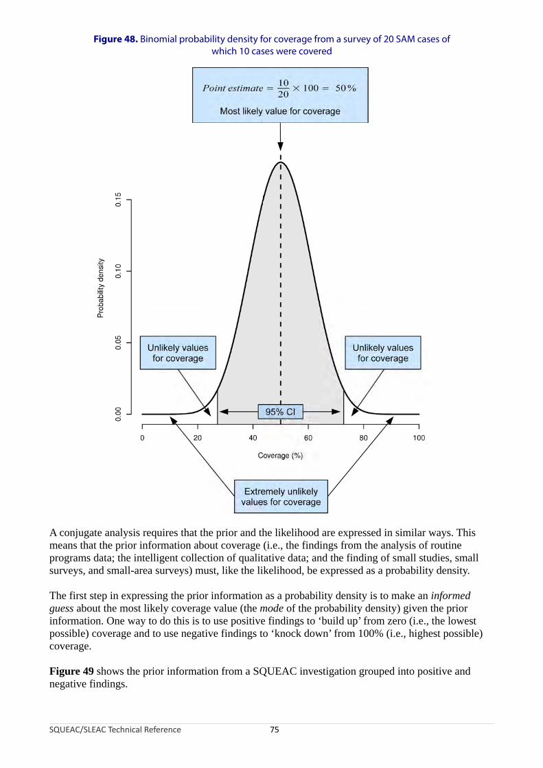
Figure 48. Binomial probability density for coverage from a survey of 20 SAM cases of which 10 cases were covered
A conjugate analysis requires that the prior and the likelihood are expressed in similar ways. This means that the prior information about coverage (i.e., the findings from the analysis of routine programs data; the intelligent collection of qualitative data; and the finding of small studies, small surveys, and small-area surveys) must, like the likelihood, be expressed as a probability density.
The first step in expressing the prior information as a probability density is to make an informed guess about the most likely coverage value (the mode of the probability density) given the prior information. One way to do this is to use positive findings to ‘build up’ from zero (i.e., the lowest possible) coverage and to use negative findings to ‘knock down’ from 100% (i.e., highest possible) coverage.
Figure 49 shows the prior information from a SQUEAC investigation grouped into positive and negative findings.
SQUEAC/SLEAC Technical Reference 75

Positive Findings Negative Findings
Finding
Scores
Finding
Scores
Simple Weighted Simple Weighted
Self-referrals 5% 5% Poor interface with SFP 5% 5%
Referrals from the community:
Carers of previous patients
Village leaders
Traditional healers
TBAs
5% 5%Lack of formal involvement of traditional healers and TBAs for case-finding and referral
5% 5%
Timely treatment seeking (admission MUAC)
5% 5% Poor remuneration of CBVs 5% 3%
Program indicators:
High proportion cured
Low mortality
Low defaulting
5% 5%Lack of oedema a sign in program messages and training of CBVs
5% 3%
Reduction of stigma associated with malnutrition
5% 3% Declining trends in admissions 5% 3%
Active cadre of CBVs 5% 3% SUM OF SCORES 25% 19%
Spatial homogeneity (small-area surveys)
5% 3%
Coverage questions (from carer interviews)
5% 1%
Short waiting times/efficient patient flow at program sites
5% 1%
Admissions respond by season 5% 1%
SUM OF SCORES 50% 32%
Data courtesy of World Vision International
Figure 49. Prior information from a SQUEAC investigation grouped into positive and negative findings with simple and weighted scores
SQUEAC/SLEAC Technical Reference 76

The simplest approach to deciding the mode of the prior is to score all findings equally (labelled ‘Simple’ in Figure 49, which uses a score of 5 for all findings). The positive scores are added together. The sum of the negative scores is subtracted from 100%. The average of the two resulting numbers is then taken. Using the ‘Simple’ scores presented in Figure 49:
50 % + (100% − 25%) 50 % + 75 %Prior Mode = = = 62.5%
2 2
Another approach to deciding the mode of the prior is to use scores or weights that reflect the relative importance or likely effect on coverage of each finding (labelled ‘Weighted’ in Figure 49, which uses scores between 1 and 5 to denote importance or the likely effect of each finding). The positive scores are added together. The sum of the negative scores is subtracted from 100%. The average of the two resulting numbers is then taken. Using the ‘Weighted’ scores presented in Figure 49:
32% +(100% − 19%) 32 % + 81 %Prior Mode = = = 56.5%
2 2
The ‘Weighted’ approach requires a more thorough review of the prior information than the simpler method. The principal advantage of this approach is that it is likely to yield a more credible value for the mode of the prior than the simpler method. This approach does not involve any extra work, because ranking of findings by their relative importance is something that will need to be done for reporting purposes.
It should be noted that these methods can produce silly results (i.e., prior modes below 0% or above 100%). For example, with an investigation with 24 positive results and 3 negative results all receiving a score of 5, this method would give an impossible value for the prior mode of:
120% +(100% − 15%) 120% + 85%Prior Mode = = = 102.5%
2 2
In cases such as this, the maximum score could be scaled so that neither the sum of positive scores or the sum of negative scores can exceed 100%. In the example given above a suitable maximum score might be:
Maximum score = ⌊10024 ⌋= 4
Using a maximum score of 4 gives:
96 % + (100% − 12 %) 96 %+ 88 %Prior Mode = = = 92%
2 2
Figure 50 presents an alternative approach to deciding the mode of the prior using estimates of program performance for key processes associated with coverage (i.e., recruitment, treatment seeking, defaulting).
These methods can yield a first guess at a credible value for the mode of the prior and should be reviewed by returning to the prior information and, if necessary, recalculated or adjusted. The value of the mode of the prior may be changed at any time before you start collecting data for the likelihood survey. If data from previous CSAS surveys, SLEAC surveys, or SQUEAC investigations are available then they may also be used to help decide a credible value for the mode of the prior.
SQUEAC/SLEAC Technical Reference 77

Figure 50. Deciding the mode of the prior as the product of program performance at key processes associated with program coverage
Data courtesy of UNICEF Sudan
SQUEAC/SLEAC Technical Reference 78

There is always uncertainty about the value of the prior mode. The amount of uncertainty about the mode of the prior is the same as the probable range of values of coverage that is consistent with the prior information. This is specified using:
• The minimum probable value for coverage that is consistent with the prior information
• The maximum probable value for coverage that is consistent with the prior information
A simple way of doing this is to use a fixed quantity, such as ± 25 percentage points. For example, with the prior information summarised in Figure 49, a value of 56.5% for the prior mode was decided. A suitable minimum probable value for this prior might be:
Minimum probablevalue = 56.5% − 25% = 31.5%
A suitable maximum probable value for this prior might be:
Maximum probable value = 56.5% + 25% = 81.5%
If there is very little uncertainty about the value of the prior mode then ± 20 percentage points might be used. It is seldom appropriate (and particularly in a program’s first SQUEAC investigation) to use a smaller value than ± 20 percentage points when specifying uncertainty about the prior mode.
There is no requirement that the distribution of the prior be symmetrical about its mode. If, for example, the maximum probable value of 81.5% calculated above is considered to be extremely unlikely (i.e., it is considered extremely unlikely that coverage could be as high as 81.5%) then it could be replaced with a more credible value (e.g., 75%).
Another situation when a symmetrical prior is likely to be unsuitable is when coverage is expected to be either very low or very high. If, for example, coverage is expected to be about 20% then values for the minimum and maximum probable values of 10% and 40% might be specified.
Note that coverage cannot be below 0% or above 100%. This means that the minimum probable value cannot be below 0% and the maximum probable value cannot be above 100%.
Another way of deciding minimum and maximum probable values is to draw a histogram prior:
1. Draw x and y axes. Label the x axis ‘Coverage’ and mark a scale of 0% to 100% in 10% intervals (decades). Label the y axis ‘Probability’ or ‘Belief’.
2. Mark the prior mode with a tall column.
3. Mark the extremely unlikely values with horizontal lines close to the x axis.
4. Mark the relative (i.e., to the prior mode) probability of coverage for each remaining decade.
5. Draw a smooth line that captures the shape of the histogram.
6. Mark the position of the minimum and maximum probable values.
This process is illustrated in Figure 51. In this example, the prior mode is about 55% and the minimum and maximum probable values are about 25% and 80%, respectively.
When deciding suitable values to describe the prior, it is important to be realistic about the strength of the prior information. The use of a narrow range of probable values should only be used when there is very little uncertainty about coverage. The mode and the minimum and maximum probable values of the prior distribution should be credible and reflect the prior information, not wishful thinking.
SQUEAC/SLEAC Technical Reference 79
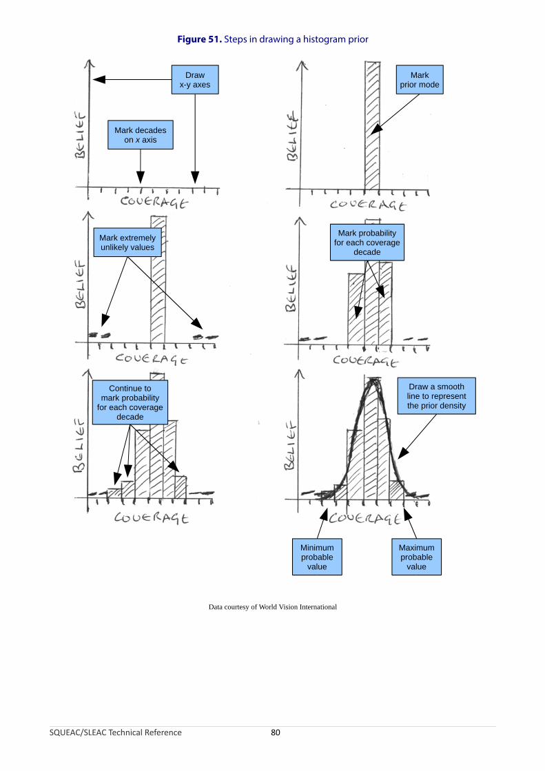
Figure 51. Steps in drawing a histogram prior
Data courtesy of World Vision International
Drawx-y axes
Markprior mode
Mark decadeson x axis
Draw a smoothline to representthe prior density
Minimumprobable
value
Maximumprobable
value
Mark extremelyunlikely values
Mark probabilityfor each coverage
decade
Continue tomark probability
for each coveragedecade
SQUEAC/SLEAC Technical Reference 80

The conjugate analysis method used in SQUEAC requires the distribution of the prior to be summarised by two numbers called shape parameters, which are labelled αPrior and βPrior. Suitable values for αPrior and βPrior may be calculated using the mode and the minimum probable value and maximum probable value of the prior with the following formulas:
minimum + 4 × mode + maximumμ =6
maximum − minimumσ =6
αPrior = μ ×(μ × (1 − μ)σ2 − 1)
(μ × (1 − μ)βPrior =(1 −μ) ×
σ 2 − 1)It should be noted that these formulas require values to be expressed as proportions, not percentages.
To convert a percentage to a proportion:
PercentageProportion =
100
For example, 55% expressed as a proportion is:
55 = 0.55100
Applying the formulas for calculating αPrior and βPrior to a prior with a mode of 55% and the minimum and maximum probable values of 25% and 80% (from Figure 51) yields:
0.25 + 4 × 0.55 + 0.80μ = = 0.546
0.80 − 0.25σ = = 0.096
0.54 × (1 − 0.54)αPrior = 0.54 × ( − 1
0.0081 )= 16.02
βPrior =(1 − 0.54)× (0.54 ×(1 − 0.54)−1)= 13.65
0.0081
A prior distribution created using these αPrior and βPrior is shown in Figure 52. Note how similar this is to the prior distribution in the histogram prior (Figure 51).
SQUEAC/SLEAC Technical Reference 81

25% 55% 80%
Figure 52. The Beta(16.02, 13.65) prior
The formulas for calculating αPrior and βPrior given above provide approximate values. The approximate values produced by these formulas are, however, accurate enough for practical purposes.
Table 4 shows approximate values for αPrior and βPrior for different prior modes at two different levels of uncertainty (i.e., ± 25 percentage points and ± 20 percentage points) calculated using these formulas. The values given in Table 4 are likely to be useful in the majority of SQUEAC investigations.
When deciding a suitable range for the prior, it is important to be realistic about the strength of the prior information. In SQUEAC investigations, values of αPrior and βPrior above 35 are likely to be inappropriately high. Values of αPrior and βPrior that are much above 35 should be used only when you are very certain about the true value of program coverage and will usually only be appropriate after a series of SQUEAC investigations or if coverage has been been estimated by a reasonably recent CSAS survey or classified by a reasonably recent SLEAC survey.
SQUEAC/SLEAC Technical Reference 82

Table 4. Approximate values for αPrior and βPrior for different prior modes at two different levels of uncertainty
SQUEAC/SLEAC Technical Reference 83
Uncertainty
± 25 percentage points ± 20 percentage points
Prior mode αPrior βPrior αPrior βPrior
20% 7.0 28.0
25% 6.5 19.5 10.3 30.9
30% 8.8 20.5 13.9 32.4
35% 11.1 20.6 17.6 32.6
40% 13.4 20.1 21.2 31.8
45% 15.6 19.1 24.6 30.1
50% 17.5 17.5 27.6 27.6
55% 19.1 15.6 30.1 24.6
60% 20.1 13.4 31.8 21.2
65% 20.6 11.1 32.6 17.6
70% 20.5 8.8 32.4 13.9
75% 19.5 6.5 30.9 10.3
80% 28.0 7.0
Example of use
Prior mode : 55%
Uncertainty : ± 25%
αPrior : 19.1From table
βPrior : 15.6
The values given in the table are approximate but are accurateenough for practical purposes.

Prior information expressed using the αPrior and βPrior shape parameters can be combined with survey (likelihood) data using a conjugate analysis:
Conjugateanalysis
PRIOR POSTERIOR
LIKELIHOOD
Survey (likelihood) data can be summarised using a numerator and a denominator. For example, the formula for a simple (point) coverage estimator is:
SQUEAC/SLEAC Technical Reference 84
Coverage = Number of current cases attending the programNumber of current cases
Numerator
Denominator
A conjugate analysis combines the αPrior and βPrior shape parameters for the prior with the numerator and denominator of the likelihood survey estimator to give the posterior probability density:
Conjugateanalysis
PRIOR POSTERIORBeta(α
Prior , β
Prior) Beta(α
Prior+ numerator, β
Prior+ denominator - numerator)
LIKELIHOODBinomial(denominator, numerator)
The posterior probability density is:
Posterior = Beta prior numerator, prior denominator − numerator
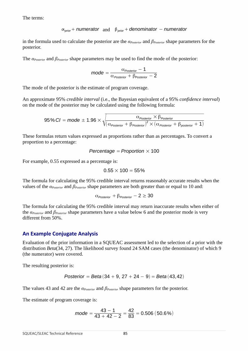
The terms:
prior numerator and priordenominator − numerator
in the formula used to calculate the posterior are the αPosterior and βPosterior shape parameters for the posterior.
The αPosterior and βPosterior shape parameters may be used to find the mode of the posterior:
αmode = Posterior − 1
αPosterior + βPosterior − 2
The mode of the posterior is the estimate of program coverage.
An approximate 95% credible interval (i.e., the Bayesian equivalent of a 95% confidence interval) on the mode of the posterior may be calculated using the following formula:
α ×β95% CI = mode ± 1.96 ×√ Posterior Posterior
(α 2Posterior + βPosterior ) × (αPosterior + βposterior + 1)
These formulas return values expressed as proportions rather than as percentages. To convert a proportion to a percentage:
Percentage =Proportion × 100
For example, 0.55 expressed as a percentage is:
0.55 × 100 = 55%
The formula for calculating the 95% credible interval returns reasonably accurate results when the values of the αPosterior and βPosterior shape parameters are both greater than or equal to 10 and:
αPosterior +βPosterior − 2 ≥ 30
The formula for calculating the 95% credible interval may return inaccurate results when either of the αPosterior and βPosterior shape parameters have a value below 6 and the posterior mode is very different from 50%.
An Example Conjugate Analysis
Evaluation of the prior information in a SQUEAC assessment led to the selection of a prior with the distribution Beta(34, 27). The likelihood survey found 24 SAM cases (the denominator) of which 9 (the numerator) were covered.
The resulting posterior is:
Posterior = Beta 34 9, 27 24 − 9 = Beta 43,42
The values 43 and 42 are the αPosterior and βPosterior shape parameters for the posterior.
The estimate of program coverage is:
43 − 1 42mode = = = 0.506 (50.6%)
43 + 42 − 2 83
SQUEAC/SLEAC Technical Reference 85
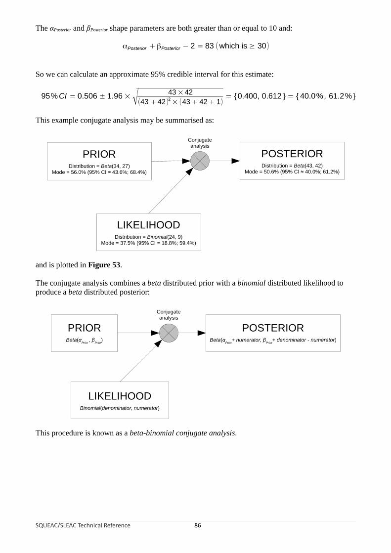
The αPosterior and βPosterior shape parameters are both greater than or equal to 10 and:
αPosterior +βPosterior − 2 = 83 (which is ≥ 30)
So we can calculate an approximate 95% credible interval for this estimate:
×95%CI 0.506 ± 1.96 ×√ 43 42= 2 = {0.400, 0.612 } = { 40.0% , 61.2%}(43 + 42) × (43 + 42 + 1)
This example conjugate analysis may be summarised as:
SQUEAC/SLEAC Technical Reference 86
PRIORDistribution = Beta(34, 27)
Mode = 56.0% (95% CI ≈ 43.6%; 68.4%)
LIKELIHOODDistribution = Binomial(24, 9)
Mode = 37.5% (95% CI = 18.8%; 59.4%)
POSTERIORDistribution = Beta(43, 42)
Mode = 50.6% (95% CI ≈ 40.0%; 61.2%)
Conjugateanalysis
and is plotted in Figure 53.
The conjugate analysis combines a beta distributed prior with a binomial distributed likelihood to produce a beta distributed posterior:
Conjugateanalysis
PRIOR POSTERIORBeta(α
Prior , β
Prior) Beta(α
Prior+ numerator, β
Prior+ denominator - numerator)
LIKELIHOODBinomial(denominator, numerator)
This procedure is known as a beta-binomial conjugate analysis.
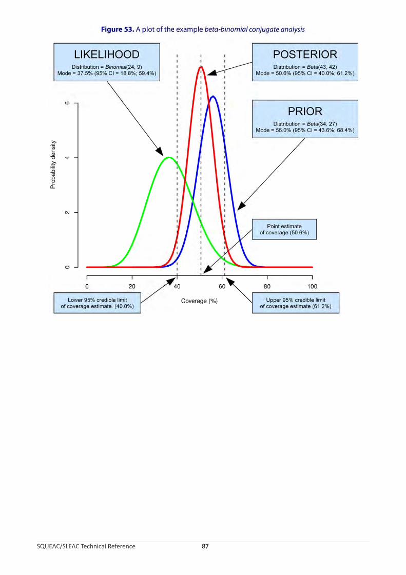
SQUEAC/SLEAC Technical Reference 87

All of the calculations required for a beta-binomial conjugate analysis may be performed using a simple pocket calculator with a square-root function (Figure 54).
Figure 54. Pocket calculator with square-root function
Beta-Binomial Conjugate Analysis Software
An open-source software package called BayesSQUEAC may also be used to perform a beta-binomial conjugate analysis. This software was designed for use in SQUEAC investigations and performs all the calculations required for a beta-binomial conjugate analysis:
• Figure 55 shows the example beta-binomial conjugate analysis being performed using the BayesSQUEAC software.
• Figure 56 shows a sample size calculation (i.e., for the likelihood survey) being performed using the BayesSQUEAC software (see page 97).
SQUEAC/SLEAC Technical Reference 88
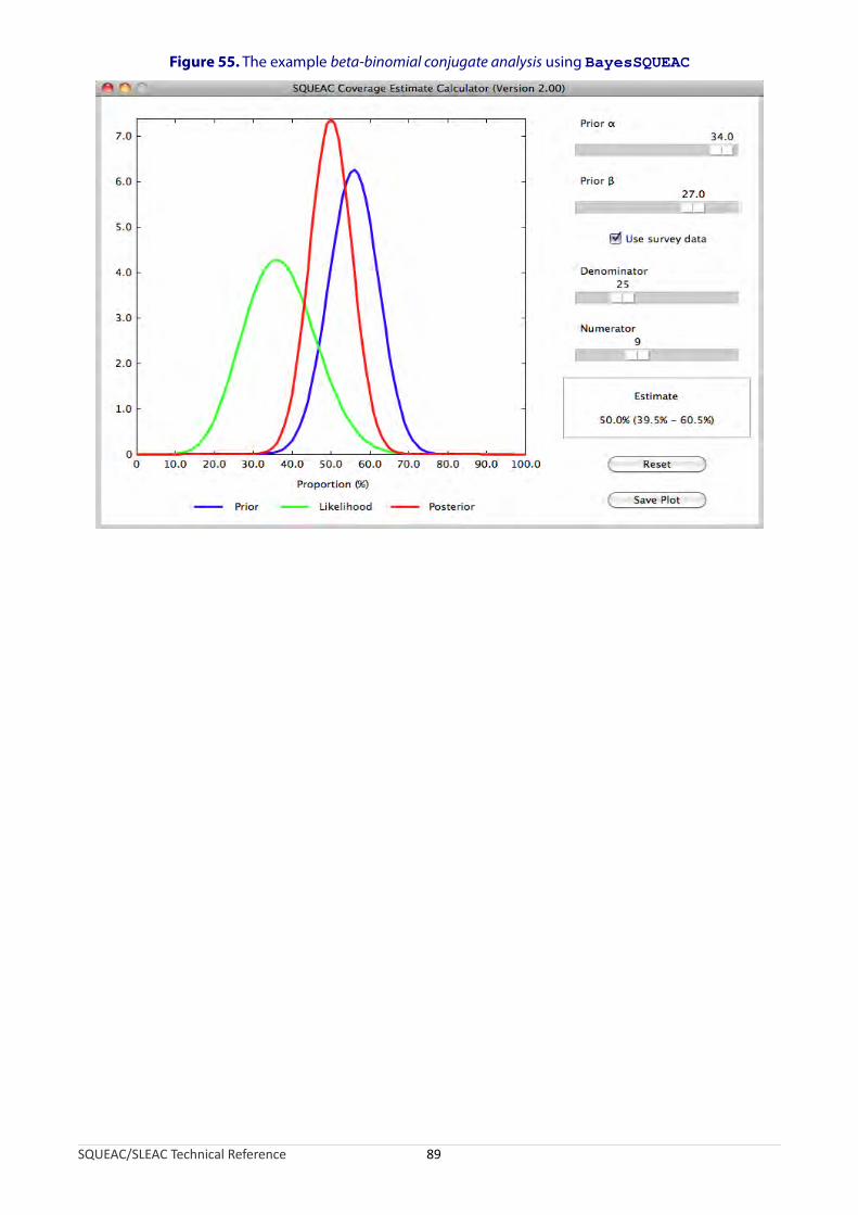
Figure 55. The example beta-binomial conjugate analysis using BayesSQUEAC
SQUEAC/SLEAC Technical Reference 89

Figure 56. Using BayesSQUEAC to calculate the sample size required to estimate coverage with a precision of ± 10% using a Beta(29, 13) prior using the simulation approach
Different numerators and denominators are tried until the displayed estimate shows the required precision
The BayesSQUEAC software also simplifies the process of performing a beta-binomial conjugate analysis by:
• Allowing the specification of the prior as a curve that matches the shape of a histogram prior without the need to calculate the αPrior and βPrior shape parameters.
• Automatic calculation of the posterior mode and 95% credible interval.
• Production of summary/diagnostic plots of the beta-binomial conjugate analysis.
• Allowing calculation of the likelihood sample size by simulation.
The BayesSQUEAC software is available for free from:
http://www.brixtonhealth.com/bayessqueac.html
SQUEAC/SLEAC Technical Reference 90
Diagnosing Coverage Estimates
It is important to realise that the beta-binomial conjugate analysis method used in SQUEAC has an important limitation. If the sample size used for the likelihood survey is small and the prior is both inaccurate and strong then the prior will dominate the analysis and the resulting coverage estimate will be biased (i.e., inaccurate). An inaccurate prior is one in which the mode of the prior is very different from the the true coverage proportion. The tendency is for the prior to overestimate coverage. This mistake is common when investigating the coverage of your own programs. It is also commonly made by inexperienced SQUEAC investigators who tend to favour evidence from program staff over other evidence from other sources. A strong prior is one with a narrow range of probable values and large values of the αPrior and βPrior shape parameters. The use of a narrow range of probable values should only be used when there is very little uncertainty about coverage and is almost never appropriate in the first SQUEAC investigation of a program.
The sample size that can be collected for the likelihood survey is limited by prevalence and the time and resources available. This means that the only way to avoid this bias problem is to be scrupulous when specifying the prior. This means being realistic about the position of the prior mode and realistic about how much the prior information can tell you about coverage. If you are unsure about the position of the prior mode then you should specify a weak prior with a wide range of probable values by using small values for the αPrior and βPrior shape parameters.
You will only know if you have specified a prior that is both inaccurate and strong after you have analysed the data. If you find that coverage estimated from the likelihood data alone using:
NumeratorCoverageLikelihood = × 100
Denominator
is very different from the position of the prior mode then the prior and the likelihood are said to conflict and the results of the beta-binomial conjugate analysis should be treated with caution.
The BayesSQUEAC software automatically produces a summary/diagnostic plot of the beta-binomial conjugate analysis. If there is little or no overlap between the distributions of the prior and the likelihood then the prior and likelihood conflict (see Figure 57). Note that the posterior is of similar width to the prior when the prior and the likelihood conflict. This means that the likelihood survey has not reduced uncertainty about coverage (i.e., it was a waste of time and resources).
There is nothing that you can do to fix the problem if the prior and the likelihood conflict other than report the problem or start the survey from scratch with a more realistic prior and collect new data. It is better, therefore, to avoid the problem by being scrupulous when specifying the prior.
SQUEAC/SLEAC Technical Reference 91
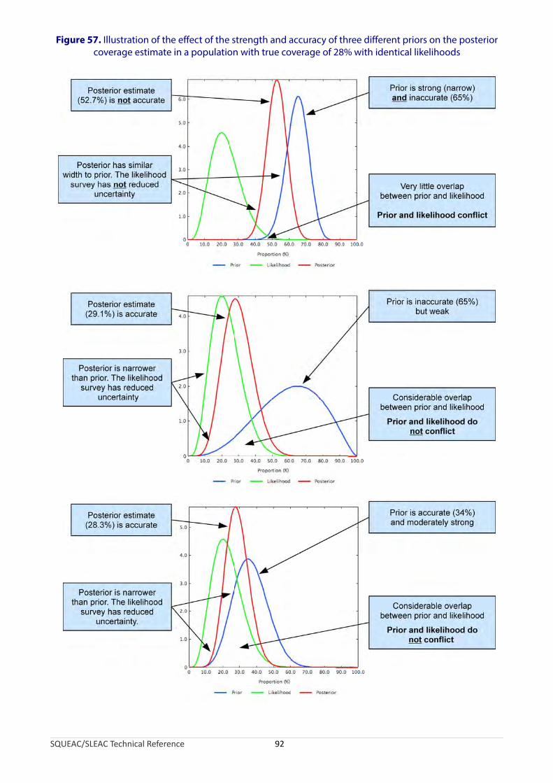
Figure 57. Illustration of the effect of the strength and accuracy of three different priors on the posterior coverage estimate in a population with true coverage of 28% with identical likelihoods
SQUEAC/SLEAC Technical Reference 92
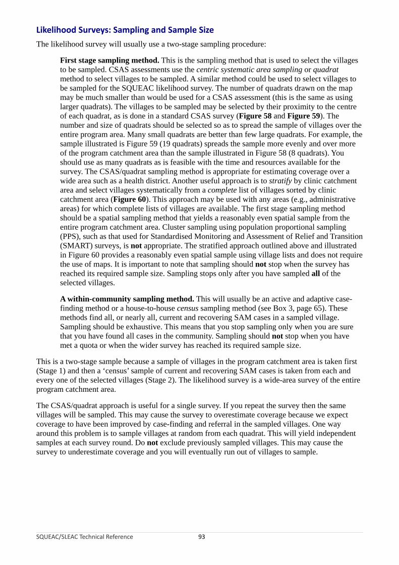
Likelihood Surveys: Sampling and Sample Size
The likelihood survey will usually use a two-stage sampling procedure:
First stage sampling method. This is the sampling method that is used to select the villages to be sampled. CSAS assessments use the centric systematic area sampling or quadrat method to select villages to be sampled. A similar method could be used to select villages to be sampled for the SQUEAC likelihood survey. The number of quadrats drawn on the map may be much smaller than would be used for a CSAS assessment (this is the same as using larger quadrats). The villages to be sampled may be selected by their proximity to the centre of each quadrat, as is done in a standard CSAS survey (Figure 58 and Figure 59). The number and size of quadrats should be selected so as to spread the sample of villages over the entire program area. Many small quadrats are better than few large quadrats. For example, the sample illustrated is Figure 59 (19 quadrats) spreads the sample more evenly and over more of the program catchment area than the sample illustrated in Figure 58 (8 quadrats). You should use as many quadrats as is feasible with the time and resources available for the survey. The CSAS/quadrat sampling method is appropriate for estimating coverage over a wide area such as a health district. Another useful approach is to stratify by clinic catchment area and select villages systematically from a complete list of villages sorted by clinic catchment area (Figure 60). This approach may be used with any areas (e.g., administrative areas) for which complete lists of villages are available. The first stage sampling method should be a spatial sampling method that yields a reasonably even spatial sample from the entire program catchment area. Cluster sampling using population proportional sampling (PPS), such as that used for Standardised Monitoring and Assessment of Relief and Transition (SMART) surveys, is not appropriate. The stratified approach outlined above and illustrated in Figure 60 provides a reasonably even spatial sample using village lists and does not require the use of maps. It is important to note that sampling should not stop when the survey has reached its required sample size. Sampling stops only after you have sampled all of the selected villages.
A within-community sampling method. This will usually be an active and adaptive case-finding method or a house-to-house census sampling method (see Box 3, page 65). These methods find all, or nearly all, current and recovering SAM cases in a sampled village. Sampling should be exhaustive. This means that you stop sampling only when you are sure that you have found all cases in the community. Sampling should not stop when you have met a quota or when the wider survey has reached its required sample size.
This is a two-stage sample because a sample of villages in the program catchment area is taken first (Stage 1) and then a ‘census’ sample of current and recovering SAM cases is taken from each and every one of the selected villages (Stage 2). The likelihood survey is a wide-area survey of the entire program catchment area.
The CSAS/quadrat approach is useful for a single survey. If you repeat the survey then the same villages will be sampled. This may cause the survey to overestimate coverage because we expect coverage to have been improved by case-finding and referral in the sampled villages. One way around this problem is to sample villages at random from each quadrat. This will yield independent samples at each survey round. Do not exclude previously sampled villages. This may cause the survey to underestimate coverage and you will eventually run out of villages to sample.
SQUEAC/SLEAC Technical Reference 93

Figure 58. A coarse CSAS/quadrat sample of villages
Intended catchment
Major road
Towns and villages
Sampling locations
Legend
SQUEAC/SLEAC Technical Reference 94
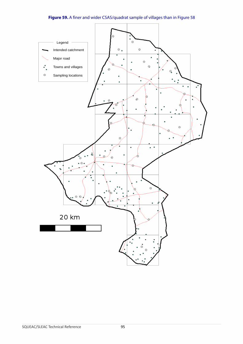
Figure 59. A finer and wider CSAS/quadrat sample of villages than in Figure 58
Intended catchment
Major road
Towns and villages
Sampling locations
Legend
SQUEAC/SLEAC Technical Reference 95
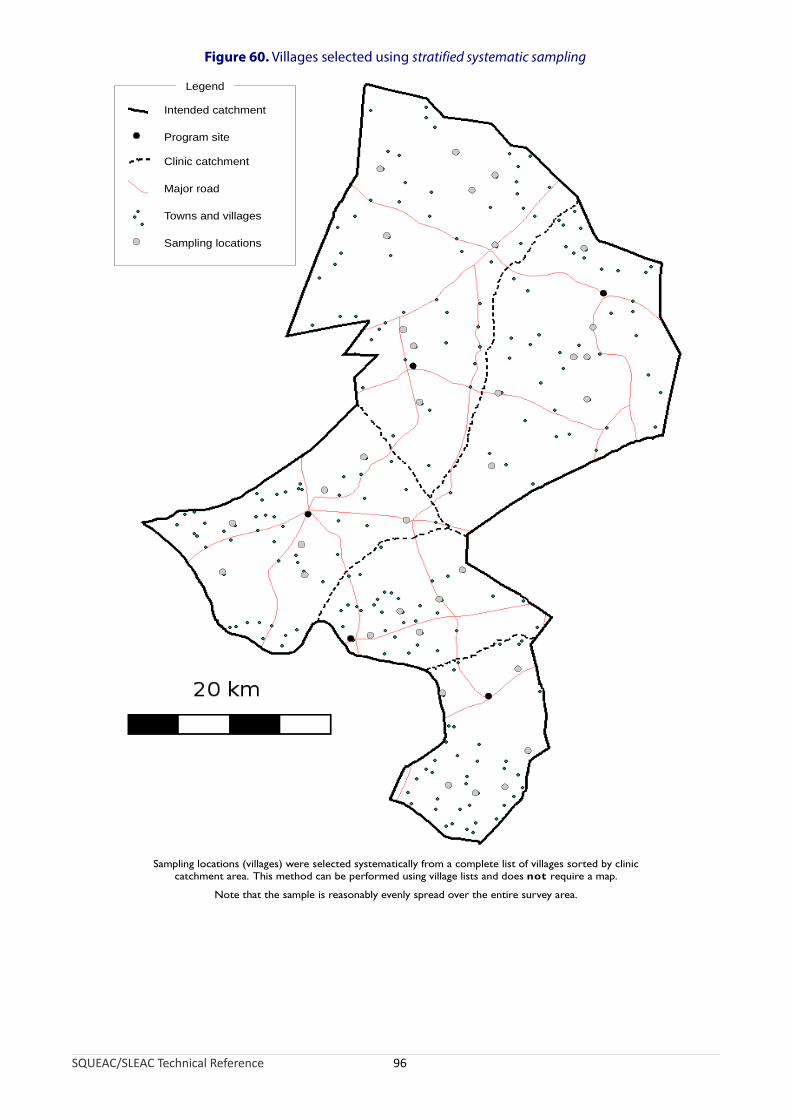
Figure 60. Villages selected using stratified systematic sampling
Intended catchment
Major road
Towns and villages
Sampling locations
Legend
Clinic catchment
Program site
Sampling locations (villages) were selected systematically from a complete list of villages sorted by cliniccatchment area. This method can be performed using village lists and does not require a map.
Note that the sample is reasonably evenly spread over the entire survey area.
SQUEAC/SLEAC Technical Reference 96

The sample size required for a likelihood survey depends on the prior and the precision required for the posterior estimate and can be calculated using the following formula:
mode ×(1 −mode )nLikelihood =⌈ (precision ÷ 1.96)2
− (αPrior +βPrior − 2)⌉where mode is the mode of the prior, αPrior and βPrior are the shape parameters of the prior, and precision is the precision required for the posterior estimate.
The ⌈ and ⌉ symbols mean that you should round up the number between the ⌈ and ⌉ symbols to the nearest whole number. For example:
⌈ 24.5 ⌉ = 25
It should be noted that this formula requires mode and precision values to be expressed as proportions, not percentages.
For example, estimating coverage with a precision of ± 10% using a Beta(29, 13) prior with a mode of 70% would require a likelihood survey with a sample size:
0.7 ×(1 − 0.7)nLikelihood =⌈ 29
( ÷ 1.96)2−( + 13 − 2)
0.1 ⌉= 41
Sample sizes for likelihood surveys are usually calculated to achieve a precision of ± 10 percentage points or better on the posterior estimate. This is the same precision as provided by the Expanded Program of Immunisation (EPI) vaccine coverage survey method. It is common practice to specify broader precisions (e.g., ± 15 percentage points or even ± 20 percentage points) and use smaller sample sizes when populations are sparse or small and the prevalence of SAM is low. In these contexts, it will be very difficult to collect a large sample and the sample size of the likelihood survey will be decided by what can be collected with the time and resources available for the survey.
The precision of the posterior estimate can be improved by increasing the sample size of the likelihood survey or by using a stronger prior (i.e., a prior with larger αPrior and βPrior shape parameters). It is only legitimate to use a stronger prior if you collect more data that allows you to specify a stronger prior. It is never legitimate to use a stronger prior to increase precision of the posterior estimate without collecting more data.
It is a good idea to use a minimum sample size of about:
nmin = αPrior + βPrior − 2
Using the example above:
nmin = αPrior +βPrior − 2
nmin = 29 + 13 − 2 = 40
Since 40 is less than or equal to 41, it would be safe, in this example, to use n = 41 in the likelihood survey.
SQUEAC/SLEAC Technical Reference 97

The purpose of this minimum sample size guideline is to ensure that the sample size of the likelihood survey is sufficiently large to be able to correct a poorly specified prior. Since a prior defined as Beta(αPrior, βPrior) is equivalent to a survey with a sample size of:
n = αPrior + βPrior − 2
the formula for nmin:
nmin = αPrior + βPrior − 2
ensures that the likelihood is at least as strong as the prior.
It is important to apply the minimum sample size guideline when there is considerable uncertainty about the accuracy of the prior (which should also be reflected in small values of αPrior and βPrior shape parameters of the prior).
If you are using a prior with small values of αPrior and βPrior and will be analysing data by hand using the formulas presented above then you should check that your survey sample size is likely to result in values of αPosterior and βPosterior that are greater than or equal to 10:
⌊ αPrior + mode × nLikelihood ⌋ ≥ 10 and ⌊ βprior + nLikelihood − mode × nLikelihood ⌋≥ 10
You should also check that:
αPrior + βprior + nLikelihood − 2 ≥ 30
If, for example, you are using a Beta(5, 7) prior that has a mode of 40% then a sample size of at least n = 20 is required since:
⌊ 5 + 0.4 × 20 ⌋ = 13 and ⌊ 7 + 20 − 0.4 × 20 ⌋ = 19 and 5 + 7 + 20 − 2 = 30
The purpose of this minimum sample size guideline is to ensure that the formula for calculating the 95% credible interval returns reasonably accurate results.
BayesSQUEAC can be used to calculate sample sizes using a simulation approach:
• The prior is specified using the ‘Prior α’ and ‘Prior β’ sliders.
• The expected survey data (i.e., different numerators and denominators) are simulated so that:
numerator ≈ demominator × prior mode
A convenient way of doing this is to change the sample size using the ‘Denominator’ slider and then change the numerator using the ‘Numerator’ slider so that the modes of the prior and the likelihood coincide. This is usually much quicker than calculating the numerator for each change in the denominator.
• Different numerators and denominators are tried systematically until the displayed estimate shows the required precision. The denominator at this point is the required sample size.
Figure 56 shows BayesSQUEAC being used to calculate a sample size to estimate coverage with a precision of ± 10% using a Beta(29, 13) prior with a mode of 70%.
SQUEAC/SLEAC Technical Reference 98
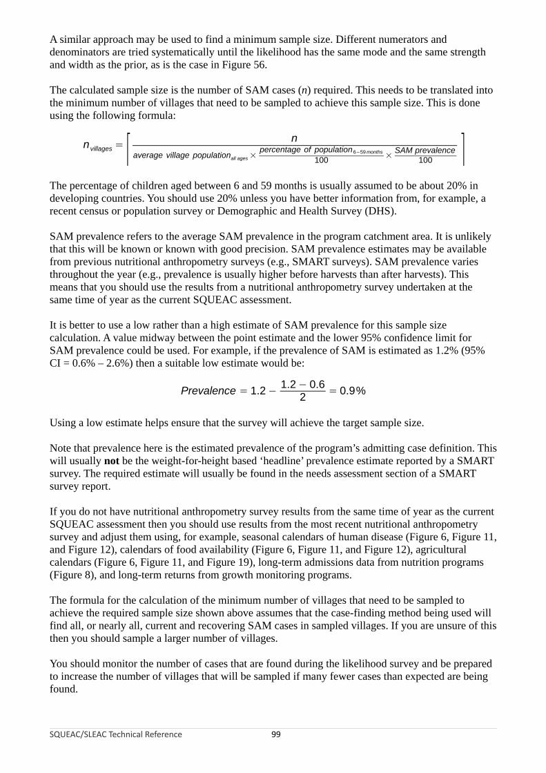
A similar approach may be used to find a minimum sample size. Different numerators and denominators are tried systematically until the likelihood has the same mode and the same strength and width as the prior, as is the case in Figure 56.
The calculated sample size is the number of SAM cases (n) required. This needs to be translated into the minimum number of villages that need to be sampled to achieve this sample size. This is done using the following formula:
nvillages = ⌈ npercentage of population
average village population 6 – 59 months SAM prevalenceall ages × ×
100 100 ⌉The percentage of children aged between 6 and 59 months is usually assumed to be about 20% in developing countries. You should use 20% unless you have better information from, for example, a recent census or population survey or Demographic and Health Survey (DHS).
SAM prevalence refers to the average SAM prevalence in the program catchment area. It is unlikely that this will be known or known with good precision. SAM prevalence estimates may be available from previous nutritional anthropometry surveys (e.g., SMART surveys). SAM prevalence varies throughout the year (e.g., prevalence is usually higher before harvests than after harvests). This means that you should use the results from a nutritional anthropometry survey undertaken at the same time of year as the current SQUEAC assessment.
It is better to use a low rather than a high estimate of SAM prevalence for this sample size calculation. A value midway between the point estimate and the lower 95% confidence limit for SAM prevalence could be used. For example, if the prevalence of SAM is estimated as 1.2% (95% CI = 0.6% – 2.6%) then a suitable low estimate would be:
1.2 − 0.6Prevalence = 1.2 − = 0.9%
2
Using a low estimate helps ensure that the survey will achieve the target sample size.
Note that prevalence here is the estimated prevalence of the program’s admitting case definition. This will usually not be the weight-for-height based ‘headline’ prevalence estimate reported by a SMART survey. The required estimate will usually be found in the needs assessment section of a SMART survey report.
If you do not have nutritional anthropometry survey results from the same time of year as the current SQUEAC assessment then you should use results from the most recent nutritional anthropometry survey and adjust them using, for example, seasonal calendars of human disease (Figure 6, Figure 11, and Figure 12), calendars of food availability (Figure 6, Figure 11, and Figure 12), agricultural calendars (Figure 6, Figure 11, and Figure 19), long-term admissions data from nutrition programs (Figure 8), and long-term returns from growth monitoring programs.
The formula for the calculation of the minimum number of villages that need to be sampled to achieve the required sample size shown above assumes that the case-finding method being used will find all, or nearly all, current and recovering SAM cases in sampled villages. If you are unsure of this then you should sample a larger number of villages.
You should monitor the number of cases that are found during the likelihood survey and be prepared to increase the number of villages that will be sampled if many fewer cases than expected are being found.
SQUEAC/SLEAC Technical Reference 99
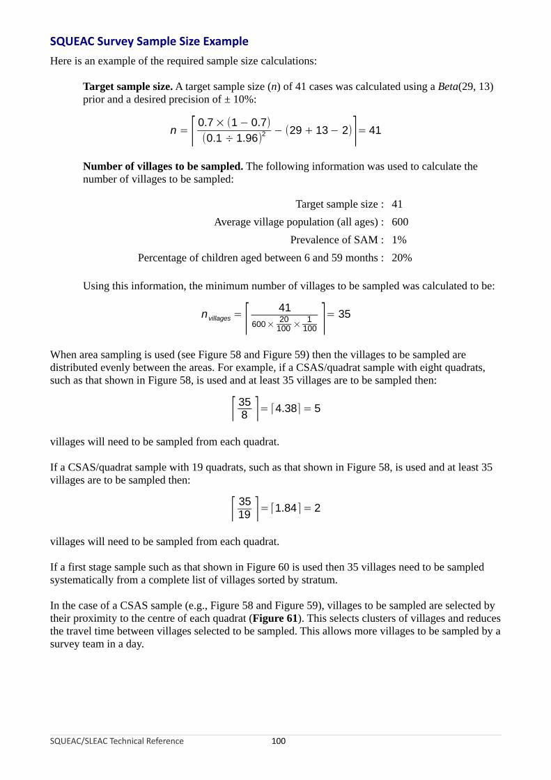
SQUEAC Survey Sample Size Example
Here is an example of the required sample size calculations:
Target sample size. A target sample size (n) of 41 cases was calculated using a Beta(29, 13) prior and a desired precision of ± 10%:
n = ⌈ 0.7 × (1 − 0.7)− (29 + 13− 2) = 41
(0.1 ÷ 1.96)2 ⌉Number of villages to be sampled. The following information was used to calculate the number of villages to be sampled:
Target sample size : 41
Average village population (all ages) : 600
Prevalence of SAM : 1%
Percentage of children aged between 6 and 59 months : 20%
Using this information, the minimum number of villages to be sampled was calculated to be:
nvillages = ⌈ 41 =20 1 35600 × ×100 100 ⌉
When area sampling is used (see Figure 58 and Figure 59) then the villages to be sampled are distributed evenly between the areas. For example, if a CSAS/quadrat sample with eight quadrats, such as that shown in Figure 58, is used and at least 35 villages are to be sampled then:
⌈ 35 ⌉= ⌈4.38⌉ = 58
villages will need to be sampled from each quadrat.
If a CSAS/quadrat sample with 19 quadrats, such as that shown in Figure 58, is used and at least 35 villages are to be sampled then:
⌈ 3519 ⌉= ⌈1.84 ⌉ = 2
villages will need to be sampled from each quadrat.
If a first stage sample such as that shown in Figure 60 is used then 35 villages need to be sampled systematically from a complete list of villages sorted by stratum.
In the case of a CSAS sample (e.g., Figure 58 and Figure 59), villages to be sampled are selected by their proximity to the centre of each quadrat (Figure 61). This selects clusters of villages and reduces the travel time between villages selected to be sampled. This allows more villages to be sampled by a survey team in a day.
SQUEAC/SLEAC Technical Reference 100
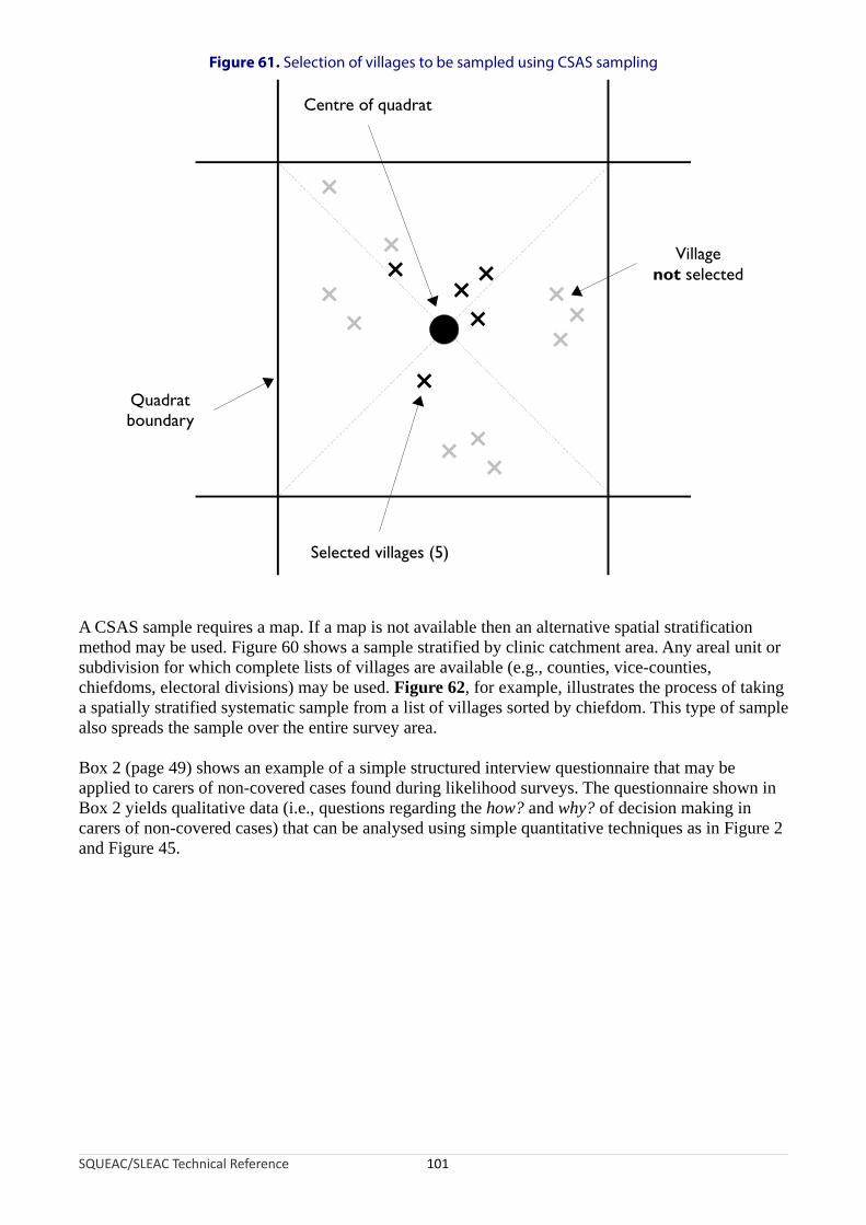
Figure 61. Selection of villages to be sampled using CSAS sampling
Quadratboundary
Villagenot selected
Selected villages (5)
Centre of quadrat
×××
×
×
×××
××
×
××
×
×
A CSAS sample requires a map. If a map is not available then an alternative spatial stratification method may be used. Figure 60 shows a sample stratified by clinic catchment area. Any areal unit or subdivision for which complete lists of villages are available (e.g., counties, vice-counties, chiefdoms, electoral divisions) may be used. Figure 62, for example, illustrates the process of taking a spatially stratified systematic sample from a list of villages sorted by chiefdom. This type of sample also spreads the sample over the entire survey area.
Box 2 (page 49) shows an example of a simple structured interview questionnaire that may be applied to carers of non-covered cases found during likelihood surveys. The questionnaire shown in Box 2 yields qualitative data (i.e., questions regarding the how? and why? of decision making in carers of non-covered cases) that can be analysed using simple quantitative techniques as in Figure 2 and Figure 45.
SQUEAC/SLEAC Technical Reference 101
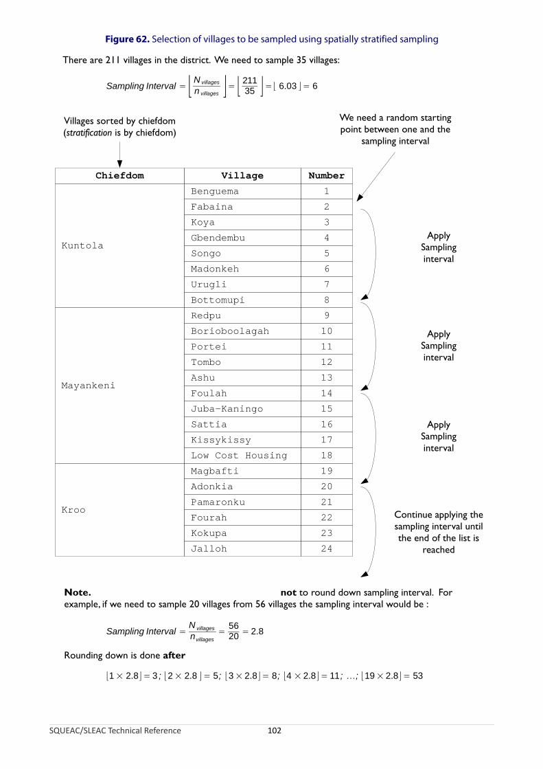
Figure 62. Selection of villages to be sampled using spatially stratified sampling
SQUEAC/SLEAC Technical Reference 102
1
2
3
4
5
6
7
8
9
10
11
12
13
14
15
16
17
18
19
20
21
22
23
24
Benguema
Fabaina
Koya
Gbendembu
Songo
Madonkeh
Urugli
Bottomupi
Redpu
Borioboolagah
Portei
Tombo
Ashu
Foulah
Juba-Kaningo
Sattia
Kissykissy
Low Cost Housing
Magbafti
Adonkia
Pamaronku
Fourah
Kokupa
Jalloh
Kuntola
Mayankeni
Kroo
Chiefdom Village Number
Villages sorted by chiefdom(stratification is by chiefdom)
We need a random startingpoint between one and the
sampling interval
There are 211 villages in the district. We need to sample 35 villages:
Sampling Interval = ⌊N villages
n villages ⌋= ⌊ 21135 ⌋=⌊ 6.03 ⌋ = 6
ApplySamplinginterval
ApplySamplinginterval
ApplySamplinginterval
Continue applying thesampling interval untilthe end of the list is
reached
Note. not to round down sampling interval. Forexample, if we need to sample 20 villages from 56 villages the sampling interval would be :
Rounding down is done after
Sampling Interval =N villages
nvillages=
5620 = 2.8
⌊1 × 2.8⌋ = 3 ; ⌊2 × 2.8 ⌋ = 5; ⌊3 × 2.8⌋ = 8; ⌊4 × 2.8⌋ = 11; …; ⌊19 × 2.8⌋ = 53

A Note on Generating Random Numbers
Random and systematic sampling both make use of random numbers. Random numbers can be generated by tossing a coin. Tossing a coin has two outcomes (i.e., heads and tails) and the method of generating random numbers by tossing a coin works by using powers of 2.
Here are some powers of 2:
Power of 2 Value Power of 2 Value
20 1 26 64
21 2 27 128
22 4 28 256
23 8 29 512
24 16 210 1024
25 32 211 2048
Each power of 2 is double the previous number so, for example, 212 = 2048 × 2 = 4096.
To generate a random number between 1 and x by tossing coins, you must work out how many coin tosses are needed. This is the smallest power of 2 that is greater than or equal to x. If, for example, you need to generate a random number between 1 and 28, you would use 25 (32) since this is the smallest power of 2 that is greater than or equal to 28. This power of 2, in this case 5, is the number of coin tosses (t) required to generate a random number between 1 and 28.
Write down powers of two starting at 20 and stopping at 2t - 1. For example:
1 2 4 8 16 Write down powers of 2 starting at 20 andstopping at 2t - 1.
Toss a coin t times and record the result of the tosses below each power of 2. For example:
1 2 4 8 16
H T H H T Toss a coin t times and record the result of thetosses below each power of 2.
Replace each heads result with its associated power of 2 and replace each tails result with 0. For example:
1 2 4 8 16
H T H H T
1 0 4 8 0 Replace each head result with its associated powerof 2 and replace each tail result with 0.
SQUEAC/SLEAC Technical Reference 103

Add up these numbers and then add 1. This is the random number. For example:
1 2 4 8 16
H T H H T
1 0 4 8 0
1 + 4 + 8 + 1 = 14 Add up these numbers and then add 1.This is the random number.
If a random number generated by this method is out of range (i.e., larger than you need) then you should discard that number and start again.
Coverage Estimators
Two estimators of coverage of selective feeding programs are in common use:
Point coverage. This estimator uses data for current cases only. It is calculated using the following formula:
Number of current cases attending the programPoint coverage = Number of current cases
Period coverage. This estimator uses data for both current and recovering cases. It is calculated using the following formula:
Period Number of current and recovering cases attending the program=
coverage (Number of current and recovering cases attending the program+ Number of current cases notattending the program )
Sphere project guidelines are unclear with regard to which coverage estimator should be used.
Both estimators have value:
• The point coverage estimator provides a snapshot of program performance and places a strong emphasis on the coverage and timeliness of case-finding and recruitment.
• The period coverage estimator includes recovering cases. These are children that should be in the program because they have not yet met program discharge criteria.
SQUEAC/SLEAC Technical Reference 104

Both estimators also have problems.
The point coverage estimator can give a misleading picture of program coverage in high-coverage programs with good case-finding and recruitment and short lengths of stay. In such cases, the two estimators will yield very different results. For example, a survey found:
Number of current cases : 2
Number of current cases in the program : 0
Number of current cases not in the program : 2
Number of recovering cases in the program : 34
The point coverage estimator returns:
0Point coverage = = 0= 0%2
but the period coverage estimator returns:
0+ 34Period coverage = = 0.944 = 94.4%0 + 34 + 2
In this example, the point coverage estimate penalises good performance, and the period coverage estimator is probably the better indicator of program coverage.
On the other hand, the period coverage estimator can give a misleading picture of program coverage in programs with poor case-finding and recruitment and long lengths of stay due to late presentation and/or late admission. In such cases, the two estimators will yield very different results. For example:
Number of current cases : 12
Number of current cases in the program : 3
Number of current cases not in the program : 9
Number of recovering cases in the program : 22
The point coverage estimator returns:
3Point coverage = = 0.250 = 25.0%12
but the period coverage estimator returns:
3 + 22Period coverage = = 0.735 = 73.5%
3 + 22 + 9
In this example, the point coverage estimator is probably the better indicator of program coverage.
The overall coverage estimate varies with the estimator used and results can be difficult to interpret without contextual information.
SQUEAC/SLEAC Technical Reference 105

Reporting Overall Coverage Estimates
The choice of estimator to report should be informed by context:
• If the program has good case-finding and recruitment and short lengths of stay then the period coverage estimator is likely to be appropriate.
• If the program has poor case-finding and recruitment and long lengths of stay due to late presentation and/or late admission then the point coverage estimator is likely to be appropriate.
You should decide which estimator is most appropriate to report and report that indicator. You should justify the selection of point or period coverage estimator in the body of the report with reference to findings regarding case-finding and recruitment and lengths of stay. You should only report the most appropriate estimator. It is not legitimate to report both estimators. It is not legitimate to pick the estimator on the basis of it yielding the higher coverage estimate.
It should be noted that a natural definition of program coverage would be:
Number of current and recovering cases attending the programProgram coverage = Total number of current and recovering cases
The denominator (i.e., the total number of current and recovering cases) in this definition is, however, difficult to collect accurately. The exclusion of recovering cases not in the program from the denominator of the period coverage estimator causes it to overestimate coverage, particularly when there are a large number of recovering cases that are not in the program, as will be the case in programs with high levels of defaulting.
It is tempting to place considerable emphasis on the overall coverage estimate from a SQUEAC investigation when reporting results. This emphasis is usually inappropriate:
• The overall coverage estimate varies with the estimator used, and estimates can be misleading (see above) and results may be difficult to interpret without contextual information.
• Overall coverage is the average coverage across the entire survey area. It conveys no information about the spatial pattern of coverage. If there is considerable spatial variation (patchiness) in coverage then the average can be misleading. Figure 1, for example, shows a map from a CSAS survey of the point coverage in a program with (generally) low and patchy coverage:
• The overall point coverage found for this program was 17.6%.
• Zero coverage was found in 8 of the 26 (31%) quadrats surveyed.
• Coverage in 16 of the 26 (62%) quadrats surveyed differed from the overall coverage estimate by more than 15 percentage points.
Figure 63 shows the distribution of per-quadrat point coverage presented in Figure 1:
• Coverage is close to the overall estimate in only about one-fifth of the areas (quadrats) surveyed.
SQUEAC/SLEAC Technical Reference 106

Figure 63. Distribution of per-quadrat point coverage found by the survey reported in Figure 1
Data courtesy of Save the Children (UK)
Both a program in which overall coverage is 17.6% but is not patchy and a program in which overall coverage is 17.6% and is patchy are failing programs, but will probably need very different reforms to improve coverage. Overall coverage results should, therefore, be accompanied by some indication of the patchiness of coverage.
If coverage is patchy, it is reasonable to not estimate overall program coverage and report the results of small-area surveys and present a map showing areas of probable high and low coverage areas.
Data collected in SQUEAC investigations include:
• Maps of home locations of beneficiaries (Figure 21 and Figure 25)
• Maps of recent outreach activity (Figure 22)
• Tabular analyses of outreach activities (Figure 23)
• Maps of homes locations of defaulting cases (Figure 24 and Figure 25)
• Tabular analysis of distance on admissions and defaulters (Table 1, page 31; and Table 2, page 32)
• Time-to-travel plots (Figure 26 and Figure 27)
• Comparison of expected and observed time-to-travel (Figure 28)
• Catchment mapping (Figure 31)
• Maps of DNA rates (Figure 35)
• Results from small-area surveys and small surveys
SQUEAC/SLEAC Technical Reference 107
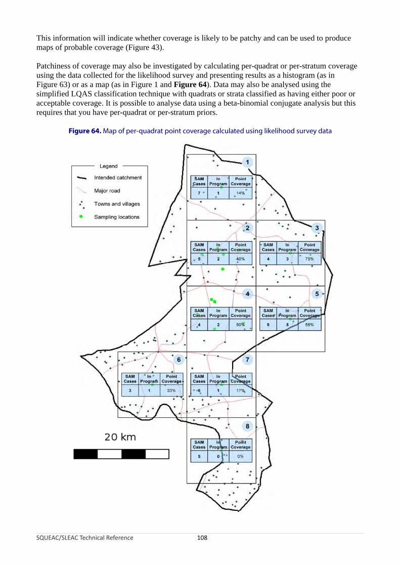
This information will indicate whether coverage is likely to be patchy and can be used to produce maps of probable coverage (Figure 43).
Patchiness of coverage may also be investigated by calculating per-quadrat or per-stratum coverage using the data collected for the likelihood survey and presenting results as a histogram (as in Figure 63) or as a map (as in Figure 1 and Figure 64). Data may also be analysed using the simplified LQAS classification technique with quadrats or strata classified as having either poor or acceptable coverage. It is possible to analyse data using a beta-binomial conjugate analysis but this requires that you have per-quadrat or per-stratum priors.
Figure 64. Map of per-quadrat point coverage calculated using likelihood survey data
SQUEAC/SLEAC Technical Reference 108
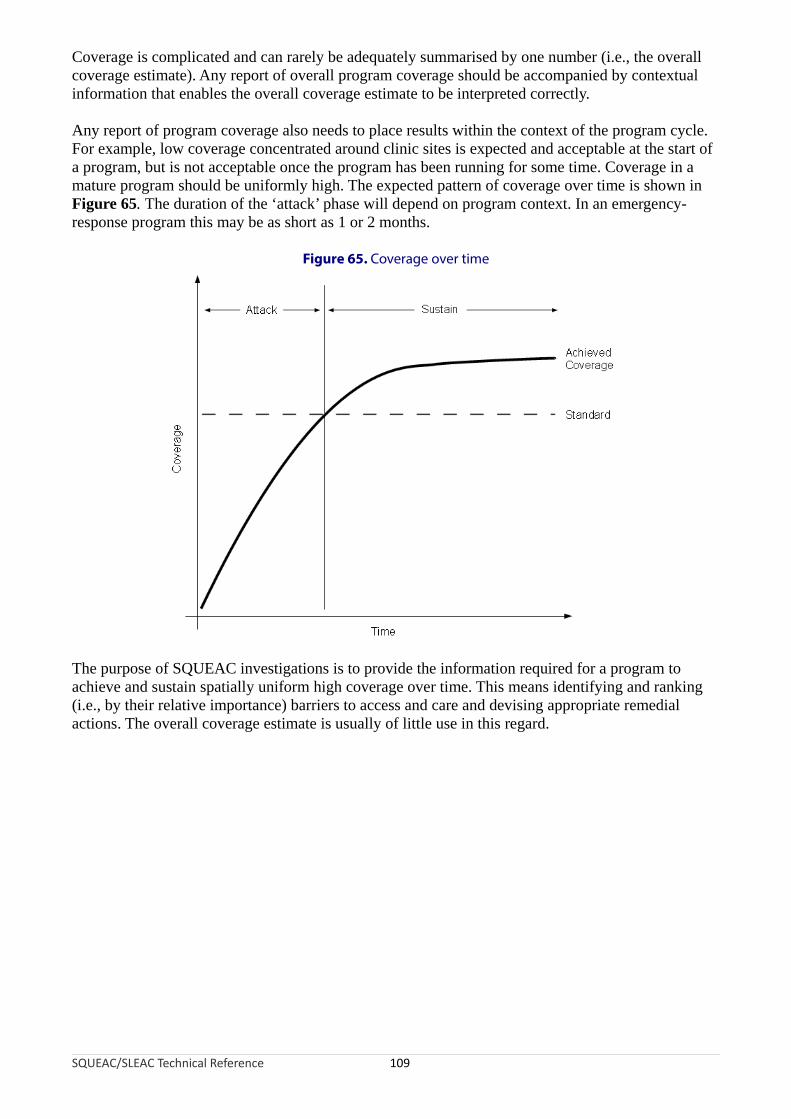
Coverage is complicated and can rarely be adequately summarised by one number (i.e., the overall coverage estimate). Any report of overall program coverage should be accompanied by contextual information that enables the overall coverage estimate to be interpreted correctly.
Any report of program coverage also needs to place results within the context of the program cycle. For example, low coverage concentrated around clinic sites is expected and acceptable at the start of a program, but is not acceptable once the program has been running for some time. Coverage in a mature program should be uniformly high. The expected pattern of coverage over time is shown in Figure 65. The duration of the ‘attack’ phase will depend on program context. In an emergency-response program this may be as short as 1 or 2 months.
Figure 65. Coverage over time
SQUEAC/SLEAC Technical Reference 109
The purpose of SQUEAC investigations is to provide the information required for a program to achieve and sustain spatially uniform high coverage over time. This means identifying and ranking (i.e., by their relative importance) barriers to access and care and devising appropriate remedial actions. The overall coverage estimate is usually of little use in this regard.
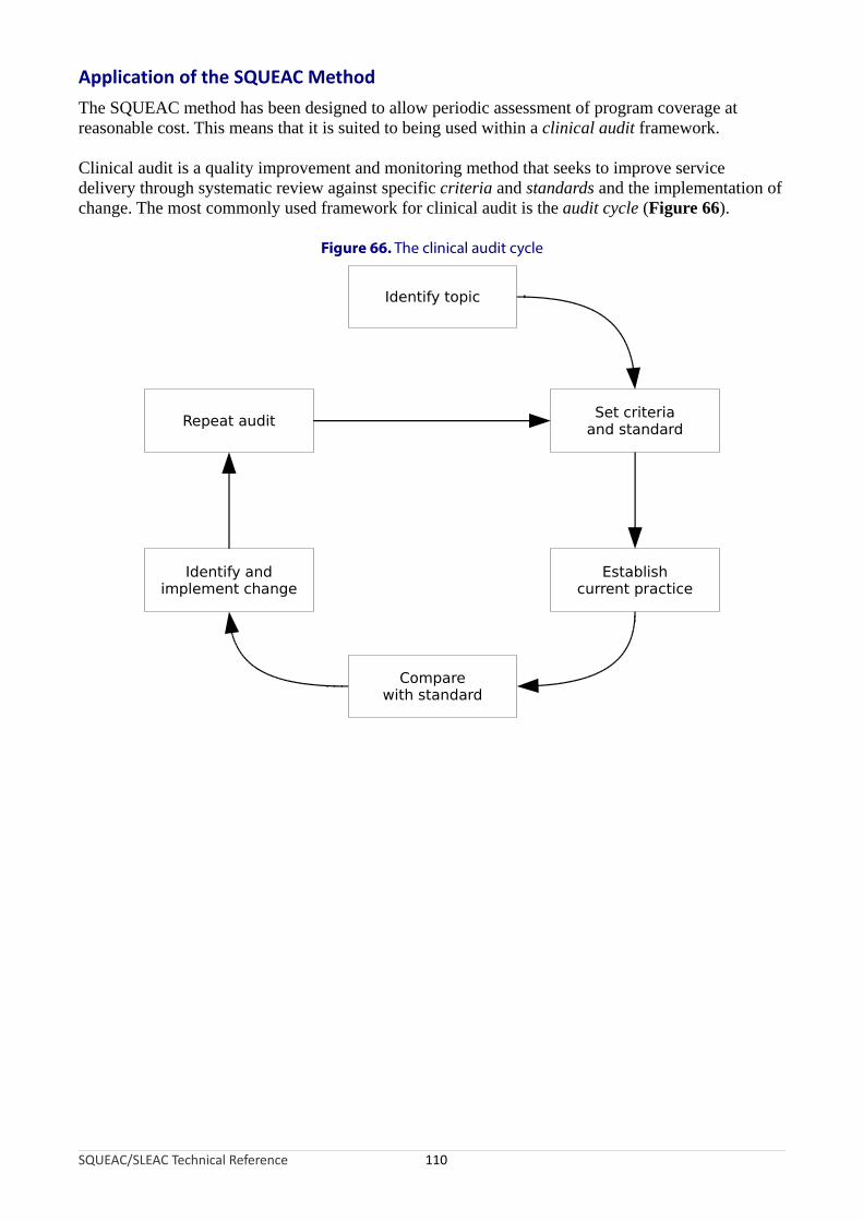
Application of the SQUEAC Method
The SQUEAC method has been designed to allow periodic assessment of program coverage at reasonable cost. This means that it is suited to being used within a clinical audit framework.
Clinical audit is a quality improvement and monitoring method that seeks to improve service delivery through systematic review against specific criteria and standards and the implementation of change. The most commonly used framework for clinical audit is the audit cycle (Figure 66).
Figure 66. The clinical audit cycle
SQUEAC/SLEAC Technical Reference 110
Identify topic
Comparewith standard
Repeat audit
Identify andimplement change
Set criteriaand standard
Establishcurrent practice
The six components of the audit cycle are:
Identify topic. In SQUEAC assessments, the topic is usually ‘program coverage’. In some cases, a SQUEAC investigation may focus on one aspect of a program (e.g., program outreach activities). In such cases, the topic will reflect the focus of the investigation.
Set criteria and standard. The criteria is what should be happening. In SQUEAC assessments, this is usually:
A child suffering from, or recovering from, severe acute malnutrition should be attending a therapeutic feeding program
The standard is how frequently the criteria should be happening. The standard used for SQUEAC assessments should, as a starting point, be the appropriate Sphere minimum standard (e.g., 50% coverage for a TFP in a rural setting). Sphere standards are minimum standards, and CMAM programs are capable of delivering coverage levels that are much higher than Sphere minimum standards. Initial SQUEAC assessments are likely to use the appropriate Sphere minimum standard (or a lower standard), but this standard should be increased (e.g., for coverage) or decreased (e.g., for defaulting and DNA rates) in subsequent SQUEAC assessments (i.e., once the program is consistently meeting the appropriate Sphere minimum standard). The standard used should be informed by the program cycle (see Figure 65). Initial SQUEAC investigations (i.e., during the ‘attack’ phase) may legitimately use standards lower than the Sphere minimum standards.
Establish current practice. This is done using the SQUEAC method or another method designed to classify or estimate program coverage and identify barriers to service access and uptake (e.g., CSAS, SLEAC).
Compare with standard. The results of the SQUEAC investigation are compared with the current standard.
Identify and implement change. The results of the SQUEAC investigation should indicate that the standard is not being met and why and where this is the case. The SQUEAC assessment identifies problems with the program and suggests remedial actions to be implemented.
Repeat audit. Audit is a cyclical process and SQUEAC investigations should be repeated every 3 or 4 months to investigate how effective any changes have been and whether further work is required.
The audit cycle aims to provide continual and incremental improvements to practice. This means that the standard should be increased once a previous standard has been met. The aim of clinical audit is to approach best practice over a number of audit cycles. Once best practice has been achieved (e.g., in CMAM programs in rural settings this means coverage levels of 80% or higher), the audit process continues in order to confirm that best practice is being sustained.
SQUEAC/SLEAC Technical Reference 111

Clinical Audit, SQUEAC, and the Observer Effect
SQUEAC and other coverage assessments tend to create an observer effect, with the assessment itself acting to improve program coverage in the short term regardless of whether or not remedial action has been implemented. There are many reasons for this:
• Follow-up of defaulting cases may result in some cases returning to the program.
• Follow-up of DNA cases may result in some cases attending the program for the first time.
• Outreach workers, CBVs, and other program staff may perform better when they know that their work is being assessed.
• Collection of qualitative data may have a ‘community mobilisation’ effect and increase awareness in the community with regard to the program’s existence, purpose, location, clinic days and times, and admission criteria.
• Small-area and likelihood surveys refer cases to the program from areas in which coverage was previously unsatisfactory.
SQUEAC investigations that are repeated too frequently are likely to observe these short-term improvements in program coverage and spatial reach and, mistakenly, attribute such improvements to the remedial actions implemented as a result of the assessment. It is advisable, therefore, that SQUEAC investigations are performed at intervals of no shorter than 3 or 4 months. This will allow time for the observer effect to ‘fade’ and for changes to be implemented and take effect. Analysis of, for example, the home locations of beneficiaries should be restricted to admissions in the 2 months prior to the start of the SQUEAC investigation.
The interval between SQUEAC investigations should be informed by context. In NGO-implemented emergency-response programs, remedial actions may be implemented quickly. In this context, an interval of 3 months between investigations would be reasonable. In developmental and post-emergency settings, remedial actions tends to be implemented less rapidly, and longer intervals (e.g., 6 or 12 months) between SQUEAC investigations might be reasonable. It should also be noted that, in many settings, SAM is highly seasonal and that finding cases of SAM outside of the ’hunger season’ can be both difficult and time-consuming. This means that survey-based activities are best left to SQUEAC investigations that are carried out during the ‘hunger season’. SQUEAC investigations that are carried out at other times might concentrate on program activities, such as staff training, community mobilisation, CBV recruitment and training, and program logistics.
These time frames apply to full SQUEAC investigations. Some SQUEAC activities can and should be done more frequently. For example, routine program monitoring data should be analysed and plotted on a monthly basis, short interviews and informal group discussions with carers at clinic sites can be done on a weekly or monthly basis, and discussions with outreach workers and volunteers can be done on a monthly basis. The aims of these activities is to reduce the work required for future full SQUEAC investigations and to provide a way of identifying potential problems with coverage as they occur to allow prompt remedial actions to be taken.
SQUEAC/SLEAC Technical Reference 112

Conclusions
The SQUEAC approach meets the design goals of a low-resource method for evaluating access and coverage:
• It is a suitable method for frequent and ongoing evaluation of program coverage and identification of barriers to service access and uptake. Initial SQUEAC investigations are unlikely to be quicker and cheaper than CSAS surveys. Subsequent SQUEAC investigations become both quicker and cheaper over time.
• The SQUEAC approach provides a similar or greater richness of information than the CSAS method provides (i.e., evaluation of the spatial pattern of coverage, identification of barriers to service access and uptake, and an estimate of overall program coverage).
• Adoption of the SQUEAC approach encourages the routine collection, analysis, and use of program planning and evaluation data.
• Individual components of the SQUEAC method provide information capable of informing program activities and reforms.
• The SQUEAC approach does not require the use of computers.
SQUEAC/SLEAC Technical Reference 113