the star complement technique - school of...
TRANSCRIPT

LECTURE NOTES ON
The Star Complement Technique
B. Tayfeh-Rezaie
Institute for studies in theoretical Physics and Mathematics (IPM)
P.O. Box 19395-5746, Tehran, Iran
For an updated version, visit
http://math.ipm.ac.ir/tayfeh-r/research.htm
January 3, 2009
1

1 Introduction
Star sets and star partitions were first introduced by Cvetkovic, Rowlinson and Simic in1993 as a way to study eigenspaces of graphs and also to investigate the graph isomorphismproblem [40]. Simultaneously, Ellingham [41] introduced the notion of star complement (heused the name µ-basis). Seemingly, the word star complement was first used by Rowlinsonin [32]. In 1995, the star partitions and the related notion of star bases were used in [35]to reestablish a result of Babai et al. [42] which states that the graph isomorphism can bedone in polynomial time for graphs with bounded eigenvalue multiplicities. Apparently,there has not been done much work after this result on star partitions. On the other hand,star sets and star complements have been proved to be helpful ideas and a lot of researcheshave been devoted to these topics. Mainly, they have been used to give bounds on the sizeof graphs and also to give characterizations of some well know graphs.
Let H be a graph of order t with no eigenvalue µ. The star complement techniqueis a method to construct a graph G with H as an induced subgraph and having µ as aneigenvalue of multiplicity equal to n− t (n, the order of G). H is said to be a star comple-ment for µ in G. The technique has been used for example to determine all exceptionalgraphs. Another main result asserts that if µ 6= −1, 0, then n ≤ (
t+12
)and therefore there
are a finite number of graphs G. The method has also been used to characterize some wellknown families of graphs by their star complements. The technique seems promising andhopefully more problems related to graph spectra will be resolved in the future by thismethod.
2 Orthogonal projection
We will need the notion of orthogonal projection to present an algebraic definition of starsets. Let W be a vector subspace of Rn. Let x be a vector. The projection of x on W isdefined as a vector y ∈ W such that x−y is orthogonal to any vector in W , i.e. x−y ∈ W⊥
(the inner product is the standard one). It is easily seen that the projection exists andis unique. If u1,u2, . . . ,um is an orthonormal basis for W , then the projection of x onW is given by
∑mi=1 < x,ui > ui. Note that the projection of x on Rn is itself and so if
v1,v2, . . . ,vn is an orthonormal basis for Rn, we have x =∑n
i=1 < x,vi > vi.
Let W and V be vector subspaces of Rn. Then the orthogonal projection of V onto W
is the linear map from V into W which sends any x ∈ V to its projection on W . Note thatthe kernel of this map is V ∩W⊥. Let V = Rn. Then the n by n matrix P representing the
2

orthogonal projection is a matrix whose columns are the projections of the standard basisof Rn represented also in the standard basis. Note that the columns of P span W . Let S
be a matrix whose columns form a basis for W . Then it is easy to see P = S(ST S)−1ST .Note that P 2 = P T = P .
The angle between two vectors x and y is defined as < x,y > /(|x||y|). The anglebetween x and W is defined as the angle between x and its projection on W .
3 Star sets and star complements
It is well known that a symmetric matrix of rank r has a full rank principle submatrix oforder r. A proof is given in the following lemma.
Lemma 1 Let M =
[A BT
B C
], where A and C are symmetric and the columns corre-
sponding to A constitute a basis for M . Then A is full rank.
Proof Every column of BT is a linear combination of columns of A which means thatevery row of B is a linear combination of rows of A. ¤
Let A be a real symmetric matrix whose columns and rows are indexed by {1, 2, . . . , n}and let µ be its eigenvalue. Let P be the matrix representing the orthogonal projectionof Rn onto the eigenspace E(µ). Since the columns of P span E(µ), we can choose a setof linearly independent columns of P to be a basis for E(µ). Using this we present analgebraic definition of star sets. Let e1, e2, . . . , en denote the standard orthonormal basisof Rn.
Definition A subset X of {1, 2, . . . , n} is called a star set if the vectors Pej(j ∈ X)form a basis for E(µ).
We also have a combinatorial definition of star sets.
Definition A subset X of {1, 2, . . . , n} is called a star set if the matrix obtained fromA by removing rows and columns corresponding to X does not have µ as an eigenvalue.In graph theory context, a star set for an eigenvalue µ in G is a subset X of vertices suchthat µ is not an eigenvalue of G \X. The graph G \X is called a star complement for µ
in G.
3

We now show that the two definitions are equivalent. We give it for graphs, but it alsoholds for any symmetric matrix.
Theorem 1 Each of the following is a necessary and sufficient condition for a k-subsetX of V (G) to be a star set for the eigenvalue µ of multiplicity k:
(i) Pej(j ∈ X) is a basis of E(µ).
(ii) E(µ) has a basis of eigenvectors xs(s ∈ X) such that xTs et = δst whenever s, t ∈ X.
(iii) µ is not an eigenvalue of G \X.
(iv) Rn = E(µ)⊕ V, where V =< ej : j 6∈ X >.
Proof (i) → (ii): P has a full rank principle submatrix of order k by Lemma 1. So thecorresponding columns of P (which are eigenvectors) can be transformed into the standardform. (ii) → (iii): Every column of µI −A corresponding to X is a linear combination ofcolumns not corresponding to X, so the result follows by Lemma 1. (iii) → (iv): We haveE(µ) ∩ V = 0. So the assertion follows. (iv) → (i): Let Pej(j ∈ X) be dependent. Thenthere is a nonzero vector x ∈ E(µ)⊥ such that it is zero on X. We have x = y + z, wherey ∈ E(µ) and z is zero on X. So x and y coincide on X and therefore using xy = 0, wehave x = 0, a contradiction. ¤
The existence of star sets can also be seen in other ways. Let G be graph witheigenvalue µ of multiplicity k. Then there exists a vertex v such that G \ v has eigenvalueµ of multiplicity k − 1. This is since the multiplicity of µ in G \ v is k − 1, k or k + 1 (byinterlacing theorem). Now by
P ′(G) =∑
v
P (G \ v)
it is clear that for some v, the multiplicity should be k − 1. So there exists a set X ofvertices of size k such that G \ X does not have µ as an eigenvalue. We also have thefollowing reasoning. Since µI −A has rank n− k, it has a principle submatrix µI − C oforder n− k such that C has no eigenvalue µ.
Since removing a vertex from a graph changes the multiplicity of an eigenvalue by atmost one, we have the following result.
Theorem 2 Let X be a star set for eigenvalue µ of multiplicity k in G and let S ⊆ X.Then µ is an eigenvalue of G \ S of multiplicity k − |S|.
4

Corollary 1 Let G be a graph with X and H as star set and star complement, respectively.Then for any Y ⊆ X, G \ Y has H as a star complement.
The following theorems are also straightforward.
Theorem 3 Let Y be a subset of V (G) such that G \Y does not have µ as an eigenvalue.Then there is a star set X such that X ⊆ Y .
Theorem 4 Let S be a subset of V (G) such that G\S has µ as an eigenvalue of multiplicityk − |S| (k, the multiplicity of µ). Then there is a star set X such that S ⊆ X.
4 Star partitions
This section is independent from the subsequent sections and so it may be neglected. LetA be a real symmetric matrix whose columns and rows are indexed by {1, 2, . . . , n}. LetA =
∑mi=1 µiPi be the spectral decomposition of A, where µi are distinct eigenvalues and
Pi denotes the matrix representing the orthogonal projection of Rn onto the eigenspaceE(µi). Since the columns of Pi span E(µi), we can choose a set of linearly independentcolumns of Pi to be a basis for E(µi). The question is that if we can find these bases suchthat their corresponding indices of columns partition {1, 2, . . . , n}.
Definition A partition X1∪X2∪· · ·∪Xm of {1, 2, . . . , n} is called a star partition if thevectors Piej(j ∈ Xi) form a basis for E(µi) for i = 1, . . . , m. The set of vectors Piej(j ∈ Xi)is called a star basis for E(µi) and the set of vectors Piej(j ∈ Xi) (1 ≤ i ≤ m) is called astar bases for Rn.
The motivation for investigating star bases is the graph isomorphism problem. This isnot to be discussed here.
Theorem 5 Any real symmetric matrix has a star partition.
Proof Let µ1, µ2, . . . , µm be distinct eigenvalues of real symmetric matrix A of order n.Let {R1, R2, . . . , Rm} be a partition of {1, 2, . . . , n} and let x1,x2, . . . ,xn be an orthonor-mal basis of Rn such that {xj : j ∈ Ri} is a basis of E(µi). Consider the transition matrixT = (tij) from the basis x1,x2, . . . ,xn to the standard basis e1, e2, . . . , en. So we have
ej =n∑
k=1
tkjxk.
5

Multiplying by Pi, we getPiej =
∑
k∈Ri
tkjxk.
By the multiple Laplacian expansion of det(T ), we have
det(T ) =∑{
±∏
det(Ti)}
,
where the summation is taken over all partitions of columns of T of type same as thepartition {R1, R2, . . . , Rm}. Since det(T ) 6= 0, for some partition we have that
∏det(Ti)
is nonzero, and so det(Ti) 6= 0 for all i. Now since {xj : j ∈ Ri} is a basis of E(µi), we findthat {Piej : j ∈ Ri} is a basis of E(µi) for all i and consequently the assertion follows. ¤
Example 1 A star partition for the Petersen graph is shown in Figure 1. This graph has750 distinct star partitions which fall into 10 nonisomorphic classes determined by theautomorphism of the graph [33].
tt
t t
t
t
t
t t
tXXX
¡¡
@@
»»»´
´´
´´££££££
BB
BB
BB
´´
´´
´LLLLLL ¯
¯¯¯¯¯
−2−2
1 1
−2−23
1
1 1
Figure 1: A star partition
For a discussion on star partitions in well known graphs such as complete graphs,complete bipartite graphs, cycles, paths and so on see Chapter 3 of [26].
With a slight modification in the proof of Theorem 5, we can prove a stronger result.
Theorem 6 Let X be a star set in G. Then there is a star partition consisting of X asone of its elements.
Note that one cannot always extend two star sets to a star partition. A counterexampleis the Petersen graph.
The next theorem follows immediately from Theorem 1.
6

Theorem 7 Each of the following is a necessary and sufficient condition for the partitionX1 ∪X2 ∪ · · · ∪Xm of V (G) to be a star partition:
(i) For each i, Piej(j ∈ Xi) is a basis of E(µi).
(ii) For each i, Rn = E(µi)⊕ Vi, where Vi =< ej : j 6∈ Xi >.
(iii) For each i, µi is not an eigenvalue of G \Xi.
(iv) For each i, E(µi) has a basis of eigenvectors xs(s ∈ Xi) such that xTs et = δst when-
ever s, t ∈ Xi.
The following theorem is obvious by Theorem 7(iv).
Theorem 8 If the eigenspaces of the (labeled) graphs G1 and G2 coincide for all pairs µ1i
and µ2i (1 ≤ i ≤ m), then the star partitions of G1 are precisely the star partitions of G2.
Theorem 9 Let G be a connected regular graph whose complement is also connected. Thenthey have the same star partitions.
Proof Since the adjacency matrices of G and G commute, there is a common basis ofeigenvectors. Also since both are regular and connected, the multiplicities of the eigenvaluepairs (µ,−1 − µ) and also of the pair (λmax, n − 1 − λmax) (n, the order of G) are thesame and therefore the eigenspaces coincide for all pairs and the assertion follows fromTheorem 8. ¤
Star partitions and star bases were originally introduced as a way to investigate thegraph isomorphism problem. For a graph we can associate a specific star bases which wecall canonical and it is minimal in some ordering of bases. Then it turns out that twographs are isomorphic if and only if they have the same eigenvalues and canonical starbases. Finding a star partition (and so a star bases) can be done in polynomial time. Ifthere is a polynomial time algorithm to determine the canonical star bases, then the graphisomorphism problem will be polynomial. See [33] for a comprehensive discussion of thesubject.
5 Operations on graphs
The following theorem is trivial. We state it since it is useful in finding star sets fordisconnected graphs.
7

Theorem 10 Let G = G1 + G2. Then X = X1 ∪X2 is a star set for G if and only if X1
and X2 are star sets in G1 and G2, respectively.
6 Galaxy graphs
A graph is called galaxy if all star sets for all eigenvalues are independence sets. Examplesinclude graphs with all eigenvalues being simple, stars, double stars and book graphs.Some results concerning these graphs are given in [28].
One also may consider the case where all star sets induce complete graphs.
7 Conjugate and opposite eigenvalues
Theorem 11
(i) Let µ1 and µ2 be conjugate (i. e. they have the same minimal polynomial overrationals). Then X is a star set for µ1 if and only if it is a star set for µ2.
(ii) Let µ1 and µ2 be opposite in a bipartite graph (i. e. µ1 = −µ2). Then X is a starset for µ1 if and only if it is a star set for µ2.
Proof (i) Since conjugate eigenvalues have the same multiplicity in a graph ??????????,the assertion easily follows. (ii) The eigenspace of µ2 is obtained from the eigenspace ofµ1 by negating entries in each eigenvector corresponding to one part of the vertices. Nowapply Theorem 1(ii). ¤
8 µ-rank
Let µ be an eigenvalue (of multiplicity m) of a graph G of order n. Then t = n−m is calledµ-rank of G. Note that µ-rank is equal to the eigenspace codimension of the eigenvalue µ.Also note that µ-rank is the rank of µI − A, A the adjacency matrix of G. Hence 0-rankis precisely the rank of G.
Note that if we add a vertex to a graph or remove a vertex from a graph, then themultiplicity of an eigenvalue changes by at most one. If we add a vertex to a graph, then
8

its µ-rank increases by at most 2. If we remove a vertex from a graph, then its µ-rankdecreases by at most 2.
9 Structural considerations for µ 6= −1, 0
Theorem 12 Let X be a star set and s ∈ X. Then the neighborhood of x in X is nonemptyor x is isolated and µ = 0.
Proof Suppose that the neighborhood of x in X is empty. Then H = G− (X \ {x}) hasµ as an eigenvalue of multiplicity 1. Removing x from H only changes the multiplicityof eigenvalue 0. Hence µ = 0. Now Suppose that x is adjacent to y in X. Consider aneigenvector which is 1 on y and zero on X \ {y} (Theorem 1(ii)). Then the sum of entrieson the the neighborhood of x is 1, a contradiction. ¤
This theorem is especially useful for cubic graphs since it shows that a star set in acubic graph is a union of cycles and matching.
The closed neighborhood of a vertex is the set obtained by adding the vertex itself toits neighborhood. The following is also straightforward using Theorem 1(ii).
Theorem 13 Let X be a star set and s, t ∈ X. If the neighborhoods of s and t in X arethe same, then
• s ∼ t, µ = −1 and s and t have the same closed neighborhood or
• s 6∼ t, µ = 0 and s and t have the same neighborhood.
Corollary 2 If µ 6∈ {−1, 0}, then the neighborhoods of elements of X in X are distinctand nonempty.
Corollary 3 For given t, there are only finitely many graphs of µ-rank t, where µ 6∈{−1, 0}.
Theorem 14 Let X be a star set and let the multiplicity of µ be k and k′ in G andG \X, respectively. Then there are at least k − k′ vertices in X which have a nonemptyneighborhood in X.
9

Proof For u ∈ X, let Γ(u) = {v ∼ u : v ∈ X} and Γ(u) = {v ∼ u : v ∈ X}. LetΓ(X) =
⋃u∈X Γ(u).
Let P denote the matrix representing the orthogonal projection ofRn onto the eigenspaceE(µ). From PA = µP , for u ∈ X we have
∑
v∈Γ(u)
Pev = µPeu −∑
v∈Γ(u)
Pev.
We show that these vectors µPeu −∑
v∈Γ(u) Pev span a space of dimension k − k′ andso
∑v∈Γ(u) Pev is a subspace of dimension k − k′ of space spanned by {Pej : j ∈ Γ(X)}
which yields |Γ(X)| ≥ k − k′. Consider the linear transformation
Peu → µPeu −∑
v∈Γ(u)
Pev.
It has the matrix µI−AX (AX , the adjacency matrix of G\X) in the basis Peu and sinceit has rank k − k′, the assertion follows. ¤
10 Structural considerations for µ = −1, 0
A graph is called reduced if it has no duplicated vertices, i.e. vertices with the sameneighborhood. A graph is called coreduced if it has no coduplicated vertices, i.e. verticeswith the same closed neighborhood. Note that from a given graph, we finally find a uniquegraph which is reduced (coreduced) by shrinking vertices with the same neighborhood(closed neighborhood) to one vertex step by step (the order does not matter).
Theorem 15 Let H be a star complement in graph G for µ = 0 and suppose that A, theadjacency matrix of G, is of the form
A =
(AX BT
B C
),
where C is the adjacency matrix of H. Let N = [B C]. Then G is reduced if and only ifthe columns of N are distinct.
Proof If G is reduced, then the result follows from Theorem 13. The converse is trivial.¤
10

Theorem 16 Let H be a star complement in graph G for µ = −1 and suppose that A,the adjacency matrix of G, is of the form
A =
(AX BT
B C
),
where C is the adjacency matrix of H. Let N = [B C + I]. Then G is coreduced if andonly if the columns of N are distinct and nonzero.
Proof If G is coreduced, then the result follows from Theorems 12 and 13. The converseis trivial. ¤
Corollary 4 For given t and µ = 0 (µ = −1), there are only finitely many reduced(coreduced) graphs of µ-rank t.
11 First bounds
Theorem 17 Let G be a graph of order n and µ-rank t. Then
• If µ 6= −1, 0, then n ≤ 2t + t− 1.
• If µ = 0 and G is reduced, then n ≤ 2t.
• If µ = −1 and G is coreduced, then n ≤ 2t − 1.
Proof For µ 6= −1, 0, the result follows from Corollary 2. For µ = 0 and µ = −1 theresult follows from Theorems 15 and 16, respectively. ¤
For non-integral eigenvalues, there is a linear bound given in the following theorem.
Theorem 18 Let G be a graph of order n and µ-rank t. If µ has l conjugates (l ≥ 2, if µ
is not integral) and the index of G is not equal to µ or any of its conjugates, then
n ≤ t− 1l − 1
+ t.
Proof Let µ be of multiplicity k. Then any of its conjugates is also of multiplicity k
?????????? and the assertion follows. ¤
11

12 Connectivity
In the proof of the following theorem we use the observation that a graph is connectedif and only if we can order its vertices such that each vertex (except for the first one) isadjacent to a preceding vertex.
Theorem 19 A connected graph has a connected star complement for any eigenvalue.
Proof Let A be the adjacency matrix of a connected graph G. Suppose that G is ofµ-rank t. We order the vertices such that each vertex (except for the first one) is adjacentto a preceding vertex. We now choose t columns of µI −A starting from the first columnand omitting any column which is a linear combination of the preceding columns. ByLemma 1, we obtain an induced subgraph H with no eigenvalue µ. We prove that H isconnected by showing that each vertex (except for the first one) is adjacent to a precedingvertex. Let y > 1 be a vertex of H and let j be the first vertex adjacent to it in G. Thenrow y in µI −A has −1 in the position (y, j) and has zero in all positions (y, i) for i < j.This shows that column j belongs to our selected columns and hence j is a vertex of H.¤
As a converse, we have the following.
Theorem 20 Let H be a star complement for µ 6= 0 in graph G and let X be the star set.Then
(i) If H is connected, then G is connected.
(ii) If H is 2-connected, then one of the following holds:
– G is 2-connected.
– µ 6= −1 and G has a pendant edge at a vertex of X.
– µ = −1 and G has a cut vertex v in X whose neighbors in X induce a completesubgraph which is a component of G \ v.
Proof (i) is trivial by Theorem 12.
We prove (ii). Suppose that H is 2-connected while G has a cutvertex v. By Theorem12, v ∈ X. Consider the neighborhood Γ(v) of v in X. Note that all vertices (X \ {v}) ∪
12

(X \Γ(v)) belong to a component C of G \ v. Hence the vertices of Γ(v) are distributed insome components Ci of G \ v and also probably in C. If µ 6= −1, then by Theorem 13, Ci
have only one vertex and we are done. Now let µ = −1. ?????????????????????????? ¤
13 Extension by a vertex
Theorem 21 Let G′ be a graph obtained from G by adding a new vertex v and character-istic vector b. Therefore, G′ has the adjacency matrix
A =
(0 bT
b A
),
where A is the adjacency matrix of G. Then mG′(µ) = mG(µ)+1 if and only if b ∈ EG(µ)⊥
and G′ has a µ-eigenvector which is nonzero in the new vertex.
Proof Let mG′(µ) = mG(µ) + 1. Consider a star set X for µ in G. Then X ∪ {v} isa star set for µ in G′. By Theorem 1, EG′(µ) has a basis of eigenvectors which has anidentity matrix form on X ∪ {v}. Therefore, G′ has a µ-eigenvector which is nonzero in v
and b ∈ EG(µ)⊥. The converse is similarly proved using star set and Theorem 1. ¤
14 Graph dominance
Definition A subset D of V (G) is called a dominating set if each vertex in D is adjacentto a vertex in D. A dominating set D is a location-dominating set if for any distinct pairu1, u2 ∈ D, we have Γ(u1)∩D 6= Γ(u2)∩D. The dominating number (respectively, location-dominating number) of a graph is the least cardinality of a dominating set (location-dominating set). By Theorems 12 and 13, we have the following.
Theorem 22 Let G be a graph with no isolated vertices. Then any star complement in G
is a dominating set and it is also a location-dominating set if µ 6∈ {−1, 0}.
For the proof of the following theorem, see [38].
Theorem 23 Let X be a star set for µ 6∈ {−1, 0} in a regular graph G. Let X be aminimal dominating set. Then
13

• If each vertex of X is isolated in G \X, then µ = 1 and G is a union of K2.
• If no vertex of X is isolated in G \ X, then µ = 1 and G is a union of Petersengraphs.
For more results on the connections of dominating sets with star sets, see [22].
15 Regular graphs with regular star complement
A star set X is called uniform if all vertices in X have the same number of neighbors inX. So if G is regular and X is uniform, then the star complement is also regular and wehave the following corollary. We denote the neighborhood of a vertex v in a graph G byG(v).
Theorem 24 Let X be a uniform star set in a graph G, say |G(v)∩X| = b for all v ∈ X.If µ is not a main eigenvalue of G, then G \X is regular of degree µ + b.
Proof For u ∈ X, let Γ(u) = {v ∼ u : v ∈ X} and Γ(u) = {v ∼ u : v ∈ X}.
Let P denote the matrix representing the orthogonal projection ofRn onto the eigenspaceE(µ). From PA = µP , for u ∈ X we have
∑
v∈Γ(u)
Pev = µPeu −∑
v∈Γ(u)
Pev.
Summing over X , we obtain∑
v∈X
bPev = µ∑
u∈X
Peu −∑
u∈X
duPeu,
where du denotes the degree of u in G \X. Since P j = 0, we obtain∑
u∈X
(µ− du + b)Peu,= 0
However, Peu are independent and so du = µ + b. ¤
Corollary 5 Let a r-regular graph H be a star complement for µ in a k-regular graph G
and let X be the star set. Then one of the following holds:
• µ = k, r = k − 1 and each component of G is a complete graph.
14

• r − k ≤ µ ≤ r − 1 and X induces a regular subgraph of degree µ + k − r.
For more results and examples and also a discussion on cubic graphs, see [37].
16 Reconstruction
Theorem 25 (The Reconstruction Theorem and its Converse) Let X be a set ofk vertices in a graph G and suppose that A, the adjacency matrix of G, is of the form
A =
(AX BT
B C
),
where AX is the adjacency matrix of the subgraph induced by X. Then X is a star set forµ in G if and only if µ is not an eigenvalue of C and
µI −AX = BT (µI − C)−1B.
In this situation, E(µ) consists of the vectors of the form(
x(µI − C)−1Bx
),
where x ∈ Rk and so (eu
(µI − C)−1bu
), u ∈ X
is a basis for E(µ).
Proof Let X be a star set for µ. By definition, µ is not an eigenvalue of C. We nowshow that
µI −AX = BT (µI − C)−1B.
We have
µI −A =
(µI −AX −BT
−B µI − C
).
By definition, µI −A and µI − C are of rank n− k. Therefore, there is L such that
[µI −AX −BT ] = L[−B µI − C].
So we have µI − AX = −LB and −BT = L(µI − C) and the assertion follows. For the
converse, it is sufficient to show that the vectors
(x
(µI − C)−1Bx
), where x ∈ Rk are
eigenvectors for µ in G and it is easily proved by a simple calculation. The result thenfollows from Theorem 3. ¤
15

The theorem can also be stated in the following form. It is just a statement of thecompatibility graph (see the next section).
Theorem 26 Let X be a set of k vertices in a graph G and suppose that A, the adjacencymatrix of G, is of the form
A =
(AX BT
B C
),
where AX is the adjacency matrix of the subgraph induced by X. Then X is a star setfor µ in G if and only if µ is not an eigenvalue of C and (G \ X) + u + v has µ as aneigenvalue of multiplicity 2 for every distinct pair u, v ∈ X.
Remark If µ is not an eigenvalue of a matrix C, then (µI − C)−1 is expressed as apolynomial in C (using the minimal polynomial of C). We have the following.
Lemma 2 Suppose that µ is not an eigenvalue of a matrix C with the minimal polynomial
m(x) = xd+1 + cdxd + cd−1x
d−1 + · · ·+ c1x + c0.
Thenm(µ)(µI − C)−1 = adC
d + ad−1Cd−1 + · · ·+ a1C + a0I,
where for 0 ≤ i ≤ d
ad−i = µi + cdµi−1 + cd−1µ
i−2 + · · ·+ cd−i+1.
Notation Let x and y be two column vectors of dimension equal to the order of µI−C.Then we define
< x,y >= xT (µI − C)−1y.
Remark Let bu denote the columns of B. Then we have
< bu,bv >=
µ if u = v,
−1 if u ∼ v,
0 otehrwise.
Let S = [B C − µI]. Then it is easy to see that
µI −A = ST (µI − C)−1S.
16

This implies
< su, sv >=
µ if u = v,
−1 if u ∼ v,
0 otehrwise,
where si denote the columns of S.
17 The compatibility graph
From the reconstruction theorem (Theorems 25 and 26), it is seen that if G has H asa star complement, then any induced subgraph of G containing H also has H as a starcomplement. Therefore, we need only to consider maximal graphs containing H. Forµ = 0 (µ = −1), note that if G is reduced (coreduced), then any induced subgraph of G
containing H is also reduced (coreduced) (see Theorems 15 and 16).
Let H be a graph with no eigenvalue µ and |V (H)| = t. Let C be the adjacency of H.We define the compatibility graph of H and µ as follows: The vertices are (0,1) vectorsbu of dimension t such that
< bu,bu >= µ,
and two vertices bu and bv are adjacent if and only if
< bu,bv >= −1, 0.
(For µ = 0,−1, we also have that the vectors −b are not the columns of µI − C.)
Now the problem of finding maximal graphs (reduced or coreduced in cases µ = −1, 0)having H as a star complement for eigenvalue µ is equivalent to find the maximal cliquesin the compatibility graph of H and µ.
Example 2 We find the maximal graphs for the star complement H for eigenvalue 1,where H is the pentagon 123451. From Lemma 2, we have
(I − C)−1 = 3I − C2 =
1 0 −1 −1 00 1 0 −1 −1
−1 0 1 0 −1−1 −1 0 1 0
0 −1 −1 0 1
.
We should have < bu,bu >= bTu (I − C)−1bu = 1. We denote bu by a set S, where
S is the set of corresponding nonzero value vertices in bu. A simple calculation shows
17

that S consists of a single vertex or three consecutive vertices of the pentagon. Hence,the compatibility graph has 10 vertices and is illustrated in Figure 2. The automorphismgroup of H has three orbits on maximal cliques (of orders 2,3 and 5). These determinethree maximal graphs shown in Figure 3, where the vertices of H are circled.
x
xx
x x
¯¯
¯¯
¯¯
¯¯
LLLLLLLLL
QQQ
´´
´´
´´
´´
xx
x
xx
QQQ
¯¯
¯¯
¯¯
¯¯
¯¯
¯¯
¯¯
¯
¯¯¯¯¯¯¯¯¯¯¯¯¯
´´
´´
´´
´´
´´
´´
´´
´´
´´
´´
´´
´´
´´
LLLLLLLLLLLLLLLL
LL
LL
LL
LL
LL
LLL
¤¤¤¤¤¤¤¤¤¤¤¤¤¤¤¤¤¤C
CCCCCCCCCCCCCCCCC
""
""
""
""
""
""
""
"""
bb
bb
bb
bb
bb
bb
bb
bbb
bb
bb
bb
¤¤¤¤¤¤¤
""
""
""
CCCCCCC
{1}
{2}
{3}{4}
{5}
{2, 3, 4}{3, 4, 5}
{4, 5, 1} {1, 2, 3}
{5, 1, 2}
Figure 2: The compatibility graph for the pentagon and eigenvalue 1
18 G(µ, t)
For given µ and t, we saw that the set G(µ, t) of graphs (reduced or coreduced in casesµ = 0,−1) of µ-rank t is finite (Corollaries 3 and 4). Consider the poset G(µ, t) with the
18

t
t
tt
tttt
m
m
m
mm
m
m
m m
m
m
m
m m
m
t
t
t t
t tt
´´
´´
´LLLLLL ¯
¯¯¯¯¯
,,
,,
,,
,
ll
ll
ll
l££££££
BBBBBB
££
££
££
BB
BB
BB
,,
,,,
ll
lll
,,
,,,
ll
lll
ttt
t t
t
t t
t
t
XXX
¡¡
@@
»»»´
´´
´´££££££
BB
BB
BB
´´
´´
´LLLLLL ¯
¯¯¯¯¯
(a) (b) (c)
Figure 3: The maximal graphs with C5 as a star complement for 1
induced subgraph partial order. The minimal elements of this poset are precisely graphsof order t with no eigenvalue µ. Any element has at least one induced subgraph of order t
which is a star complement for eigenvalue µ. It is easy to see that the maximal elementsof this poset are exactly those maximal graphs obtained from the compatibility graphs ofall graphs of order t with no eigenvalue µ. The compatibility graphs provide an algorithmto generate G(µ, t). Note that if G in G(µ, t), it is not true that any induced subgraph ofG is also in G(µ, t).
19 Maximal elements of G(0, t)
First we give some elementary properties of maximal elements of G(0, t). Note that suchelements always have an isolated vertex. However, we consider these elements withouttheir isolated vertices. In the following, G(u) dentes the neighborhood of u.
Lemma 3 Let G be a maximal element of G(0, t). Let u and v be two nonadjacent verticessuch G(u) ∩G(v) = ∅. Then there is a vertex w such that G(w) = G(u) ∪G(v).
Proof Trivial. ¤
This lemma shows that such elements are connected and non-bipartite (except for K2).We also have the following.
19

Lemma 4 Every maximal element of G(0, t) has diameter at most 3.
Proof Consider two vertices u and v. Then apply Lemma 3 to v and some x ∈ G(u).Then the assertion easily follows. ¤
It is shown that Kn is a maximal and at the same time a minimal element of G(0, n)[41]. Some other families of graphs which are maximal in G(0, t) are also known (see[1, 41]). Also all reduced graphs with rank at most 7 are found in [1]. For rank 8, allmaximum reduced graphs are obtained [1].
20 m(µ, t)
The maximum order of a graph in G(µ, t) is denoted by m(µ, t). In [1], it is conjecturedthat
m(0, t) =
{2(t+2)/2 − 1 if t is even,
5.2(t−3)/2 − 1 if t is odd and t > 1.
In [1, 34], by a simple construction it is shown that the above provides a lower bound form(0, t). An upper bound is given in Theorem 17. For µ 6= −1, 0, we will give a quadraticbound in the next section. However, for µ = 0, it is not possible to give a polynomialbound since there are examples of exponential orders. Here is an example: Consider areduced graph G of order n and rank t. Duplicate each vertex and add a new vertex andconnect it to one of pairs of vertices. The resulting graph G′ is of order 2n + 1 and rankt + 2. It has the adjacency matrix
A A jt
A A 0j 0 0
,
where A is the adjacency matrix of G. Starting form a single vertex we found a graphof order 2(t+2)/2 − 1 and rank t for any even t. Kotlov and Lovasz [34] have shown thatfor a reduced graph of rank t, the number of vertices is less than c2t/2 for some constantc. One question which arises is that what happens for coreduced graphs. Note that if wedrop the property of being reduced (coreduced), then the order of graph is not boundedfrom the above.
20
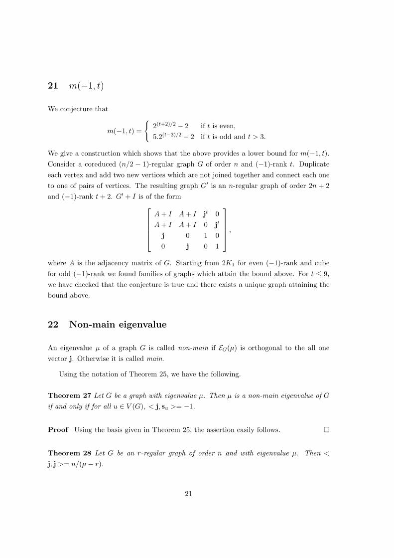
21 m(−1, t)
We conjecture that
m(−1, t) =
{2(t+2)/2 − 2 if t is even,
5.2(t−3)/2 − 2 if t is odd and t > 3.
We give a construction which shows that the above provides a lower bound for m(−1, t).Consider a coreduced (n/2 − 1)-regular graph G of order n and (−1)-rank t. Duplicateeach vertex and add two new vertices which are not joined together and connect each oneto one of pairs of vertices. The resulting graph G′ is an n-regular graph of order 2n + 2and (−1)-rank t + 2. G′ + I is of the form
A + I A + I jt 0A + I A + I 0 jt
j 0 1 00 j 0 1
,
where A is the adjacency matrix of G. Starting from 2K1 for even (−1)-rank and cubefor odd (−1)-rank we found families of graphs which attain the bound above. For t ≤ 9,we have checked that the conjecture is true and there exists a unique graph attaining thebound above.
22 Non-main eigenvalue
An eigenvalue µ of a graph G is called non-main if EG(µ) is orthogonal to the all onevector j. Otherwise it is called main.
Using the notation of Theorem 25, we have the following.
Theorem 27 Let G be a graph with eigenvalue µ. Then µ is a non-main eigenvalue of G
if and only if for all u ∈ V (G), < j, su >= −1.
Proof Using the basis given in Theorem 25, the assertion easily follows. ¤
Theorem 28 Let G be an r-regular graph of order n and with eigenvalue µ. Then <
j, j >= n/(µ− r).
21

Proof Use <∑
su, j >= −n. ¤
Theorem 29 Let G be a graph with star set X and star complement H for eigenvalue µ.Then µ is a non-main eigenvalue of G if and only if µ is a non-main eigenvalue of H + u
for all u ∈ X.
Proof We use the basis given in Theorem 25. Every eigenvector of this basis correspondsto an eigenvector of H + u for some unique u ∈ X. Therefore the assertion easily follows.¤
23 Bound on the order of graphs
The following inequality is proved using a well known technique in algebraic combinatorics:Consider a vector space of polynomials of dimension n and find a set of m independentpolynomials. Then m ≤ n.
Theorem 30 Let G 6= K2, 2K2 be a graph of order n and of µ-rank t > 1 for eigenvalueµ 6= −1, 0. Then
n ≤(
t + 12
),
and hence a star set has size at most(
t2
).
Proof Let
A =
(AX BT
B C
),
where A and AX are the adjacency matrices of A and the subgraph induced by a starset X, respectively. Let S = [B C − µI] and let su denote the columns of S. Definepolynomials Fu : Rt → R as
Fu(x) =< su,x >2
which are quadratic homogenous functions of the general form f(x1, x2, . . . , xt) =∑
cix2i +∑
dijxixj . If we prove that Fu are independent, then we have n ≤ t +(
t2
)=
(t+12
).
First we suppose that G is connected and µ is not its index. Let b = (b1, b2, . . . , bn)T
be the positive eigenvector corresponding to the index. Let b′ = (bn−t+1, b2, . . . , bn)T .Assume that
∑αuFu = 0. Let a = (α1, α2, . . . , αn)T and a′ = (α1b1, α2b2, . . . , αnbn)T .
We haveAa = −µ2a
22

andAa′ = µa′.
Since µ 6= −µ2, we have aTa′ = 0, i. e∑
α2ubu = 0 and so α1 = α2 = · · · = αn = 0.
The first relation follows from∑
αuFu(x) = 0 by letting x = si and the second relationfollows from
∑αuFu(x) = 0 by letting x = si + b′ (note that < su,b′ >= −bu by the
reconstruction Theorem).
The rest of proof is straightforward. ¤
Remark The above bound is sharp since it is attained in the following examples: (i)The unique exceptional graph of order 36 (here µ = −2 and t = 8) which is obtained fromL(K8) by switching with respect to the vertices in a clique of size 8, (ii) K3, µ = 2 and(ii) P3, µ = ±√2.
Remark A strongly regular graph attaining the absolute bound is called extremal. Theonly known extremal strongly regular graphs are pentagon, complete multipartite graphs,the Schlafli graph (27 vertices), the McLaughlin graph (275 vertices) and the complementof these two latter graphs. It is a long time standing question whether these are the onlyexamples.
Remark The bounds given in this section extend the absolute bound (which is equal tothe bound given in Theorem 32) for regular graphs and any graph in general.
Theorem 31 Let G be a graph of order n and of µ-rank t > 2 for a non-main eigenvalueµ 6= −1, 0. Then
n ≤(
t + 12
)− 1 =
12(t− 1)(t + 2).
Proof We use the notation in the proof of Theorem 30. Let
F (x) =< j,x >2 .
We show that F is not in the span of Fu. Assume by the contrary that F =∑
βuFu. Wehave
< j,x >< j,y >=∑
βu < su,x >< su,y > .
First let x = y = si to findj = (µ2I + A)b,
23

where b = (β1, . . . , βn). Then let x = si and y = j to find
< j, j > j = (µI −A)b.
From these we see that b is a constant value vector. Let βu = β. Now
β2(∑
< su,x >< su,y >)2 =< j,x >2< j,y >2= β2∑
< su,x >2∑
< su,y >2 .
From the Cauchy-Schwarz inequality, we have < su,x >= α < su,y > and so x = αywhich means that t = 1. ¤
Theorem 32 Let G be a r-graph of order n and of µ-rank t > 2 for an eigenvalue µ 6=−1, 0, r. Then
n ≤(
t + 12
)− 1 =
12(t− 1)(t + 2).
Moreover, equality holds if and only if G is an extremal strongly regular graph with µ asits eigenvalue of greatest multiplicity.
Proof The first part follows from Theorem 31. For the second part, a proof is given in[14]. We here give an easier proof. Define f(x) =< x,x > . By the proof of Theorem31, f is in the span of Fu(x) =< su,x > and F (x) =< j,x >. So we may write f =δF +
∑u εuFu. We have < x,y >= δ < j,x >< j,y > +
∑u εu < x, su >< y, su >. If
we put x = si and y = −j, then we obtain that (µI − A)ε is a constant vector, whereεt = (ε1, . . . , εn). If we evaluate f in si, then we obtain that (µ2I + A)ε is a constantvector. This shows that εu are constant. Now if put x = si and y = sj , then we find thatany two vertices have a constant number of common neighbors. ¤
Remark For µ = 0, consider (n−t)K1∪Kt and for µ = −1, consider (t−1)K1∪Kn−t+1.This shows that in these cases n is not bounded by t.
24 An application: Graph construction
Sometimes the star complement technique can be used to construct graphs with givenspectral (or topological) properties. In this approach, first the star complement is guessedand then it is possibly extended to a whole graph using the compatibility graph.
We present two successful applications of this method. One of the main achievementsin this direction was the classification of all maximal exceptional graphs (473 graphs in
24

total). A thorough treatment of the problem can be found in [11] and [15]. We only makesome comments. An exceptional graph is a connected graph with least eigenvalue at least−2 which is not a generalized line graph. It was proved many years ago that such a graphhas at most 36 vertices and has degree at most 28. All regular exceptional graphs, 187 innumber, were found very soon. Also exceptional graphs with least eigenvalue greater than−2 (573 graphs) were known in early years. However, the general problem remained openuntil it was answered recently in [17], where all maximal exceptional graphs were found.Note that any exceptional graph is an induced subgraph of a maximal exceptional graph.The classification was done by the star complement technique making an extensive use ofcomputer. The key observation was that any exceptional graph has an exceptional starcomplement with least eigenvalue greater than −2.
The other application is on extremal strongly regular graphs. Rowlinson [6] investigatessuch graphs having a maximum number of independent vertices (obtained from Cvetkovic’sTheorem). He proves that such a graph is necessarily the Schlafli graph or the McLaughlingraph.
25 The general and restricted problems
The general problem is to find all graphs having a given graph as a star complement.In other words, in the reconstruction theorem (Theorem 25), given C, we want to findAX , B, µ. The restricted problem is to find all graphs having a given graph as a starcomplement for the eigenvalue µ. In other words, in the reconstruction theorem, given C
and µ, we want to find all AX and B.
Why are these problems interesting? We can give three reasons: First it is a naturalcuriosity to try to identify the maximal graphs corresponding to nice star complements(such as complete, path, cycle, tree,...). Secondly, the maximal graphs obtained in thisway might be objects with interesting properties. Thirdly, the maximal graphs obtainedin this way provide lower bounds on the maximum order of a graph of a given µ-rank.
The known results are as follows. In the following, H is used to denote a star comple-ment.
25

25.1 Graphs with small µ-rank
The general problem has been answered for all graphs with at most 5 vertices and µ 6= −1, 0[25]. All maximal reduced graphs with rank at most 7 are obtained in [41]. In [1], thenumber of all reduced graphs with rank at most 7 is given. For rank 8, all maximumreduced graphs are found [1].
25.2 Independence set
For H = Kt, there is a simple characterization given in [32].
25.3 Star
For H = K1,s, there is a thorough discussion in [32]. Also for regular extensions, we referto [23]. The case K1,5 is teated in full generality in [24]. See also [26].
25.4 Complete bipartite graphs
For H = Kr,s, some general observations are given in [30]. Also in this reference, the caseK2,5 is treated in detail. All these and the case H = Kr,s + tK1 with a general discussionon µ, are also available at [26].
25.5 Star+isolated vertices
For H = K1,s + 2K1 (µ = 1) and H = K1,s + 2K1 (µ = −2), the maximal graphs arefound in [29]. In this reference, also the similar problem has been solved for H being agraph consisting of an isolated vertex together K2,s with a pendant edge at a vertex ofdegree s. The case H = K1,16 + 6K1 for µ = 2 is done in [26] (also presented in [16]).
25.6 Union of two paths or a path and a cycle
For H = Pr, H = Pr + Ps and H = Pr + Cs and µ = −2, the results are given in [13].Note that these types of star complements are more difficult and involved than those oftypes in the previous subsections.
26

25.7 Union of odd cycles
For H =⋃
i C2si+1, there is a complete answer in [27] and [8].
25.8 Complete graphs
For H = K8 and µ = −2, it is shown (using a computer search) that there are exactly 363maximal graphs [10].
25.9 Line graph of trees
Let T be tree. For H = L(T ) and µ = −2, the results are given in [11]. In this reference,there are also results for line graph of odd-unicyclic graphs.
25.10 Trees, unicyclic and complete graphs with 1 as the second largest
eigenvalue
See (Stanic, 2007 [4]) and (Stanic and Simic, [2]).
26 Other problems
26.1 Matching type problem
Sometimes it is interesting to find AX , µ, C for given B in Theorem 25. An example is a“matching type problem”, where B is assumed to be the identity matrix [21].
26.2 Extremal strongly regular graphs
The only known extremal strongly regular graphs are pentagon, complete multipartitegraphs, the Schlafli graph, the McLaughlin graph and the complement of these two lattergraphs. It is a long time standing question whether these are the only examples.
27

26.3 (−1)-rank
Can we make better the bound given in Theorem 17 for m(−1, t)? What can be saidabout the maximal elements of G(−1, t)?
26.4 Characterization of the well known graphs by star complement
For example Kneser graph KG(n, 2) is the unique regular graph with the star complementK1,n−3 + 2K1 for the eigenvalue 1. There are many results of this type. See for example[29]. For the Hoffman-Singleton graph, see [3].
26.5 rank
Prove the conjecture for m(0, t). Give a characterization of maximal elements in G(0, t).Give a characterization of minimal elements in G(0, t). Give a characterization of minimal-maximal elements in G(0, t).
Acknowledgments I am thankful to Professor P. Rowlinson for providing me with someof the references. I am also grateful to F. Ramezani for drawing the figures.
28

The following is a complete (?) list of papers which deal with the star
complement technique. The entries are sorted by date.
References
[1] S. Akbari, P. J. Cameron and G. B. Khosrovshahi, Ranks and signatures ofadjacency matrices, preprint.
[2] Zoran Stanic and S. K. Simic, On graphs with unicyclic star complement for 1as the second largest eigenvalue, preprint.
[3] P. Rowlinson, Some properties of the Hoffman-Singleton graph, Appl. Anal. Dis-crete Math., to appear.
[4] Zoran Stanic, On graphs whose second largest eigenvalue equals 1—the star com-plement technique, Linear Algebra Appl. 420 (2007), no. 2-3, 700–710.
[5] D. M. Cvetkovic, P. Rowlinson and S. K. Simic, Star complements andexceptional graphs, Linear Algebra Appl. 423 (2007), no. 1, 146–154.
[6] P. Rowlinson, Co-cliques and star complements in extremal strongly regular graphs,Linear Algebra Appl. 421 (2007), no. 1, 157–162.
[7] Francis K. Bell, Marzi Li, Maria Enzo and Slobodan K. Simic, Some newresults on graphs with least eigenvalue not less than −2, Rend. Sem. Mat. MessinaSer. II 9(25) (2003), 11–30 (2004).
[8] Francis K. Bell and Slobodan K. Simic, On graphs whose star complement for−2 is a path or a cycle, Linear Algebra Appl. 377 (2004), 249–265.
[9] M. I. Skvortsova and I. V. Stankevich, On a relationship between the eigen-vectors of weighted graphs and their subgraphs, Discrete Math. Appl. 14 (2004), no.6, 569–577
[10] P. Rowlinson, Star complements and maximal exceptional graphs, Publ. Inst. Math.(Beograd) (N.S.) 76(90) (2004), 25–30.
[11] D. M. Cvetkovic, P. Rowlinson and S. K. Simic, Spectral generalizationsof line graphs, On graphs with least eigenvalue −2, London Mathematical SocietyLecture Note Series, 314, Cambridge University Press, Cambridge, 2004.
29

[12] D. M. Cvetkovic and P. Rowlinson, Spectral graph theory, In: Topics in alge-braic graph theory (eds. L. W. Beinke and R. J. Wilson), Cambridge University Press,Cambridge, 2004, pp. 88-112.
[13] Francis K. Bell, Line graphs of bipartite graphs with Hamiltonian paths, J. GraphTheory 43 (2003), no. 2, 137–149.
[14] F. K. Bell and P. Rowlinson, On the multiplicities of graph eigenvalues, Bull.London Math. Soc. 35 (2003), no. 3, 401–408.
[15] Dragos Cvetkovic, Graphs with least eigenvalue −2; a historical survey and recentdevelopments in maximal exceptional graphs, Linear Algebra Appl. 356 (2002), 189–210.
[16] P. S. Jackson and P. Rowlinson, Star complements and switching in graphs,Linear Algebra Appl. 356 (2002), 135–143.
[17] D. M. Cvetkovic, M. Lepovic, P. Rowlinson and S. K. Simic, The maximalexceptional graphs, J. Combin. Theory Ser. B 86 (2002), no. 2, 347–363.
[18] P. Rowlinson, Star complements in finite graphs: a survey, 6th Workshop on Com-binatorics (Messina, 2002). Rend. Sem. Mat. Messina Ser. II 8(24) (2001/02), suppl.,145–162.
[19] D. M. Cvetkovic, P. Rowlinson and S. K. Simic, The maximal exceptionalgraphs with maximal degree less than 28, Bull. Cl. Sci. Math. Nat. Sci. Math. No.26 (2001), 115–131.
[20] D. M. Cvetkovic, P. Rowlinson and S. K. Simic, Graphs with least eigenvalue−2: the star complement technique, J. Algebraic Combin. 14 (2001), no. 1, 5–16.
[21] N. E. Clarke, W. D. Garraway, C. A. Hickman and R. J. Nowakowski,Graphs where star sets are matched to their complements, J. Combin. Math. Combin.Comput. 37 (2001), 177–185.
[22] Bolian Liu and P. Rowlinson, Dominating properties of star complements, Publ.Inst. Math. (Beograd) (N.S.) 68(82) (2000), 46–52.
[23] P. Rowlinson, Star sets in regular graphs, J. Combin. Math. Combin. Comput. 34(2000), 3–22.
30

[24] P. Rowlinson, Star sets and star complements in finite graphs: a spectral con-struction technique, Discrete mathematical chemistry (New Brunswick, NJ, 1998),323–332, DIMACS Ser. Discrete Math. Theoret. Comput. Sci., 51, Amer. Math. Soc.,Providence, RI, 2000.
[25] F. K. Bell and P. Rowlinson, Graph eigenspaces of small codimension, DiscreteMath. 220 (2000), no. 1-3, 271–278.
[26] P. S. Jackson, Star sets and related aspects of algebraic graph theory, Ph.D. thesis,University of Stirling, 1999.
[27] F. K. Bell, Characterizing line graphs by star complements, Linear Algebra Appl.296 (1999), no. 1-3, 15–25.
[28] F. K. Bell, D. M. Cvetkovic, P. Rowlinson and S. K. Simic, Some additionsto the theory of star partitions of graphs, Discuss. Math. Graph Theory 19 (1999),no. 2, 119–134.
[29] D. M. Cvetkovic, P. Rowlinson and S. K. Simic, Some characterizations ofgraphs by star complements, Linear Algebra Appl. 301 (1999), no. 1-3, 81–97.
[30] P. S. Jackson and P. Rowlinson, On graphs with complete bipartite star com-plements, Linear Algebra Appl. 298 (1999), no. 1-3, 9–20.
[31] D. M. Cvetkovic, M. Lepovic, P. Rowlinson and S. K. Simic, A databaseof star complements of graphs, Univ. Beograd. Publ. Elektrotehn. Fak. Ser. Mat. 9(1998), 103–112.
[32] P. Rowlinson, On graphs with multiple eigenvalues, Linear Algebra Appl. 283(1998), no. 1-3, 75–85.
[33] D. M. Cvetkovic, P. Rowlinson and S. K. Simic, Eigenspaces of graphs,Encyclopedia of Mathematics and its Applications, 66, Cambridge University Press,Cambridge, 1997.
[34] A. Kotlov and L. Lovasz, The rank and size of graphs, J. Graph Theory 23(1996), 185–189.
[35] D. M. Cvetkovic, Star partitions and the graph isomorphism problem, Linear andMultilinear Algebra 39 (1995), 109–132.
31

[36] D. M. Cvetkovic, P. Rowlinson and S. K. Simic, On some algorithmic investi-gations of star partitions of graphs, Partitioning and decomposition in combinatorialoptimization, Discrete Appl. Math. 62 (1995), no. 1-3, 119–130.
[37] P. Rowlinson, Star partitions and regularity in graphs, Linear Algebra Appl.226/228 (1995), 247–265
[38] P. Rowlinson, Dominating sets and eigenvalues of graphs, Bull. London Math. Soc.26 (1994), no. 3, 248–254.
[39] P. Rowlinson, Eutactic stars and graph spectra, Combinatorial and graph-theoretical problems in linear algebra (Minneapolis, MN, 1991), 153–164, IMA Vol.Math. Appl., 50, Springer, New York, 1993.
[40] D. M. Cvetkovic, P. Rowlinson and S. K. Simic, A study of eigenspaces ofgraphs, Linear Algebra Appl. 182 (1993), 45–66.
[41] M. N. Ellingham, Basic subgraphs and graph spectra, Australas. J. Combin. 8(1993), 247–265.
[42] L. Babai, D. Grigorjev and D. M. Mount, Isomorphism of graphs with boundedeigenvalue multiplicities, Proc. 14th Annual ACM symp. on the theory of computing(San Franscisco 1982), New York, (1982), 310–324.
32