the strange logic of galton-watson trees
TRANSCRIPT

The Strange Logic of Galton-Watson Trees
by
Moumanti Podder
A dissertation submitted in partial fulfillment
of the requirements for the degree of
Doctor of Philosophy
Department of Mathematics
New York University
May 2017
Professor Joel Spencer


Acknowledgements
First and foremost, I would like to acknowledge my parents, my grandpar-
ents, my aunt, uncle and cousin for being extremely supportive of my education
throughout. Their liberal outlook and interest in academia have always been an
inspiration, and they continue to support and motivate me in all my mathematical
and creative endeavours. My sincere gratitude goes out to my doctoral advisor,
Prof. Joel Spencer, and my collaborators: Prof. Tim Austin, Dr. Alexander Hol-
royd, Prof. Mihyun Kang, Prof. Maxim Zhukovski, Dr. Tobias Johnson, Dr. Fiona
Skerman, Dr. Oliver Cooley, Dr. Krishanu Maulik, Dr. Ecaterina Sava-Huss, Gun-
delinde Wiegel and Avi Levy for their valuable guidance and cooperation in our
respective joint research projects. An especially profound thanks to Prof. Spencer
for being an excellent mentor, an ingenious pedagogue and a loving father figure,
all rolled into one.
I would like to thank all my teachers from primary and high school (notably
Sharmila Ma’am, Shubhankar Sir, Sushmita Ma’am, Sumana Ma’am, Sunanda
Ma’am), my professors from undergraduate and master’s programmes at the Indian
Statistical Institute, Kolkata (notably Prof. Parthanil Roy, Prof. Alok Goswami,
Prof. Sreela Gangopadhyay), and my professors at the Courant Institute of Mathe-
matical Sciences (notably Prof. Eyal Lubetzky, Prof. Pierre Germain, Prof. Henry
McKean, Prof. Anne-Laure Dalibard, Prof. Raghu Varadhan, Prof. Yuri Bakhtin).
I would like to express my heartfelt gratitude to my closest friends, without
whose constant supply of courage and persistence I would not have gotten very
far: Subhabrata Sen, Snigdha Panigrahi, Pragya Sur, Rounak Dey, Raka Mandal,
Shrijita Bhattacharya, Sayar Karmakar, Kushal Kumar Dey, Saswati Saha, Arpita
Mukherjee, Sabyasachi Bera, Deepan Basu, Rejaul Karim among my undergradu-
iii
ate friends; Sylvester Eriksson-Bique, Reza Gheissari, Manas Rachh, Ian Tobasco,
Aukosh Jagannath, Monty Essid, Stephanie Crooks, Megan Lytle among my grad-
uate friends; Prateeti Pal, Aaheli Sengupta, Sreyoshi Mukherjee, Sreemala Das
Majumdar and Arunima Bhattacharya among others. Last but not the least, I
would like to thank my gracious landlady, Jennifer Tichenor, our previous admin-
istrator, Tamar Arnon, current administrators Melissa Kushner Vacca, Michelle K.
Shin and Betty Tsang, human resources manager Karen Micallef, and previous and
current mailmen Larry Cohen and Michael Laguerre, for all the help throughout
my stay in New York.
iv

Abstract
My dissertation is on the analysis of the probabilities of different classes of
properties, parametrized by mathematical logic, on the well-known Galton-Watson
(GW) branching porcess. Most of the results hold for very general offspring distri-
butions (with only the assumption of having exponential moments), but we mainly
work with the Poisson(λ) offspring distribution. The first part of my dissertation
focuses on probabilities of first order (FO) sentences which capture local struc-
tures inside the tree. I give a complete description of the probabilities Pλ[A] of all
possible FO sentences A conditioned on the survival of the GW tree. Here Pλ[A]
denotes the probability of A under the Galton-Watson measure induced by the
Poisson(λ) offspring distribution. There are, up to tautology, only a finite number
of FO sentences of given quantifier depth k. For an arbitrary k, I introduce a
natural distributional recursion Ψk, such that the probabilities of these sentences
form a fixed point of Ψk. I further show that Ψk is a contraction, and that its fixed
point is unique and analytic in λ.
The second part of my dissertation focuses on existential monadic second order
(EMSO) properties of the GW tree. Survival of the rooted tree is an EMSO
property. I show that finiteness of the rooted tree, the negation of survival, is not
an EMSO; furthermore, there is no EMSO which can express finiteness on all but
a measure 0 subset of trees.
The final part of my dissertation considers the alternating quantifier depths
(a.q.d.) of FO sentences. I give a specific sequence KEINs of sentences and
show that the a.q.d. of KEINs is precisely s. In particular this implies that the
a.q.d. hierarchy for this sequence does not collapse.
v
Contents
Acknowledgements . . . . . . . . . . . . . . . . . . . . . . . . . . . . . . iii
Abstract . . . . . . . . . . . . . . . . . . . . . . . . . . . . . . . . . . . . v
List of Figures . . . . . . . . . . . . . . . . . . . . . . . . . . . . . . . . . viii
Introduction . . . . . . . . . . . . . . . . . . . . . . . . . . . . . . . . . . 1
0.1 Ehrenfeucht games . . . . . . . . . . . . . . . . . . . . . . . . . . . 3
0.2 Existential monadic second order properties on rooted trees . . . . . 6
1 Analysis of first order probabilities, conditioned on the survival
of the Galton-Watson tree 10
1.1 Outline of the chapter, introduction and main results . . . . . . . . 10
1.2 Containing all finite trees . . . . . . . . . . . . . . . . . . . . . . . . 19
1.3 Universal trees exist! . . . . . . . . . . . . . . . . . . . . . . . . . . 28
1.4 Probabilities conditioned on infiniteness of the tree . . . . . . . . . 35
1.5 Extension of results to general offspring distributions . . . . . . . . 41
1.6 At criticality, under Poisson offspring distribution . . . . . . . . . . 44
2 Probabilities of first order sentences as fixed points of a contract-
ing map 46
2.1 Outline of the chapter . . . . . . . . . . . . . . . . . . . . . . . . . 46
vi
2.2 The Contraction formulation . . . . . . . . . . . . . . . . . . . . . . 55
2.3 Universality . . . . . . . . . . . . . . . . . . . . . . . . . . . . . . . 59
2.4 Unique fixed point . . . . . . . . . . . . . . . . . . . . . . . . . . . 66
2.5 A proof of contraction . . . . . . . . . . . . . . . . . . . . . . . . . 66
2.6 Implicit function . . . . . . . . . . . . . . . . . . . . . . . . . . . . 73
3 Finiteness is not almost surely an EMSO 75
3.1 Introduction and outline of the chapter . . . . . . . . . . . . . . . . 75
3.2 The description of the games . . . . . . . . . . . . . . . . . . . . . . 77
3.3 Further notions required for the proof that types game is stronger
than set-pebble Ehrenfeucht . . . . . . . . . . . . . . . . . . . . . . 80
3.4 The types game is stronger than EHR . . . . . . . . . . . . . . . . 90
3.5 Duplicator wins the type game . . . . . . . . . . . . . . . . . . . . . 108
3.6 Recursiveness of the property of being ubiquitous . . . . . . . . . . 121
4 Alternating quantifier depth of a class of recursively defined prop-
erties 123
4.1 The description of the problem . . . . . . . . . . . . . . . . . . . . 123
4.2 The specialized Ehrenfeucht game to prove this . . . . . . . . . . . 124
4.3 The inductive construction . . . . . . . . . . . . . . . . . . . . . . . 126
4.4 The inductive winning strategy for Duplicator . . . . . . . . . . . . 128
Bibliography 139
vii
List of Figures
1.1 Example of a typical neighbourhood class of the root . . . . . . . . 39
2.1 Probability of survival of the tree. . . . . . . . . . . . . . . . . . . . 48
2.2 Probability of having no node with exactly one child. . . . . . . . . 49
4.1 Trees T(s+1,k,m)1 and T
(s+1,k,m)2 . . . . . . . . . . . . . . . . . . . . . 127
4.2 Trees T(s,k,m)1 and T
(s,k,m)2 . . . . . . . . . . . . . . . . . . . . . . . . 128
4.3 T(s+1,k,m)1 with detailed view of T
(s+1,k,m)1 (um+1) . . . . . . . . . . . 131
4.4 T(s+1,k,m)2 with detailed view of T
(s+1,k,m)2 (vm+1) . . . . . . . . . . . 131
viii
Introduction
The Poisson Galton-Watson tree (henceforth, GW tree) T = Tλ with parameter
λ > 0 is a much studied object (see [3], [10] and [11]). It is a random rooted tree,
with a single root, and each node, independently, has Z children where Z follows
Poisson distribution with mean λ. We let Pλ denote the probability under Tλ. We
shall set
p∗ = p∗(λ) = Pr[Tλ is infinite]. (1)
As is well known, when λ ≤ 1, p∗ = 0 while when λ > 1, p∗ is the unique positive
solution to the equation
1− x = e−xλ. (2)
We let T ∗λ denote the process Tλ conditioned on the survival of the tree. When
examining T ∗λ , we tacitly assume λ > 1. For any property A of rooted trees, we
let Pλ[A] and P ∗λ [A] denote the probabilities of A being satisfied by Tλ and T ∗λ
respectively. In the sequel, we often drop the subscript λ, as we always work with
an arbitrary but fixed λ.
Let T be the space of all rooted trees with finite-degree nodes. For any tree
T ∈ T , we let V (T ) denote its vertex set, and its root is denoted by RT . For any
v ∈ V (T ), we let d(v) denote the depth of v in T , where d(RT ) = 0. For v ∈ V (T ),
let T (v) denote the subtree of T that is rooted at v. For any positive integer n
and any T ∈ T , let T |n denote the truncation of T , retaining up to depth n. We
call T |n the n-cutoff of T (this is defined even if no vertices are at generation s).
We can similarly define T (v)|n, and call it the n-cutoff of T (v).
In Chapters 1 and 2, we shall examine the first order language on rooted trees T .
In this language, the root RT is a constant symbol. We have two relations: equality
1
= of nodes and the parent-child relationship π (in our notation, π(v) denotes the
parent of v for all vertices v 6= RT ). Purists may prefer a binary relation π[v, w],
which denotes that w is the parent of v. Sentences must be finite and made
up of the usual Boolean connectives (¬,∨,∧, =⇒ ,⇔ etc.) and existential and
universal quantifications ∃ and ∀ over vertices. The quantifier depth of a sentence
A is the depth of the nesting of the existential and universal quantifiers. A formal
definition of quantifier depth may be found in Section 1.2 of [5], along with many
other aspects of first order logic on random structures.
We illustrate with a few examples what a typical first order sentence looks like.
Example 0.0.1. Consider the property that there exists a node in the tree that has
precisely two children. This can be expressed in first order language as follows:
∃ u[∃ v1
[∃ v2
[π(v1) = u ∧ π(v2) = u∧
[∀ v π(v) = u =⇒ (v = v1) ∨ (v = v2)]]]]
.
In this particular example, the quantifier depth is 4.
Example 0.0.2. Consider the property that the root of the tree has precisely one
child and precisely one grandchild. Observe that the root of the tree being a desig-
nated symbol, this property is written in first order language as follows:
∃ u[∃ v[π(u) = RT ∧ π(v) = u ∧ [∀ u′π(u′) = RT
=⇒ (u′ = u)] ∧ [∀ v′π(v′) = u =⇒ (v′ = v)]]].
The quantifier depth in this example is 3.
2
Example 0.0.3. Consider the property that no node in the tree has precisely one
child. This can be expressed as follows:
¬[∃ u[∃ x[π(x) = u ∧ ∀ z[π(z) = u =⇒ z = x
]]. (3)
We allude to this example once again in Chapter 2, and show a plot of the proba-
bility of this property in Figure 2.1.
We refer the reader to [5] for further discussion on first order logic.
0.0.1 Fictitious continuation:
This is a particularly useful way of viewing the Galton-Watson process that
comes in handy in both Chapters 1 and 2. Let X1, X2, . . . be a countable sequence
of mutually independent and identically distributed Poisson(λ) random variables.
Let Xi be the number of children of the i-th node, when the tree is explored using
breadth first search (the root is considered the first node so that X1 is its number
of children; siblings are labeled in a lexicographic manner). If and when the tree
terminates (this occurs when∑n
i=1Xi = n − 1 for the first time) the remaining
(fictitious) Xj are not used.
0.1 Ehrenfeucht games
The Ehrenfeucht games, also sometimes known as the Ehrenfeucht-Fraısse games,
serve as a key tool, in various forms, in all of Chapters 1 through 4. The form
in which they are used depends on the language we are investigating (first order,
existential monadic second order etc.), and the kind of problem we are concerned
3

with. However, the most standard form is commonly known as the pebble-move
Ehrenfeucht game. We introduce this form in this section, and give rough ideas
about the other forms used in Chapters 3 and 4.
The Ehrenfeucht games are what bridges the gap between mathematical logic
and a complete structural description of logical statements on rooted trees (and
other structures, such as general graphs). The pebble-move Ehrenfeucht games
are described as follows.
Definition 0.1.1. Fix an arbitrary positive integer k. The k-round pebble-move
Ehrenfeucht game is played between two players: the Spoiler and the Duplicator,
and on two given rooted trees T1 and T2. The quantities T1, T2 and k are known a
priori to both players. Each round consists of a move by the Spoiler, followed by
a move by the Duplicator. In each round, Spoiler picks a vertex from either of T1
and T2; in reply, Duplicator picks a vertex from the other tree. Let (xi, yi) denote
the pair of vertices selected from V (T1) × V (T2) in the i-th round, for 1 ≤ i ≤ k.
Unless otherwise states, we almost always adopt the following convention: we set
x0 = RT1 , y0 = RT2 . (4)
Set [k] = 0, 1, . . . k. Duplicator wins this game, which we denote byEHR[T1, T2, k],
if she can maintain both of the following conditions: for all i, j ∈ [k],
i. xi = xj ⇔ yi = yj;
ii. π(xj) = xi ⇔ π(yj) = yi.
The pebble-move Ehrenfeucht game is primarily used to analyze first order
sentences on rooted trees. We write T1 ≡k T2 if and only if Duplicator wins
4
EHR[T1, T2, k]. The relation ≡k is an equivalence relation, and it partitions the
space T of all rooted trees into finitely many equivalence classes. Let Σ = Σk
denote the set of all these equivalence classes. For any tree T , the equivalence
class to which it belongs is generally called the k-round Ehrenfeucht value of T .
In order to avoid confusion arising from different versions of the game, we shall
in particular refer to this as the pebble-move Ehrenfeucht value in Chapters 1 and
2. The following lemma sets up a crucial connection between the pebble-move
Ehrenfeucht game and first order properties on rooted trees.
Lemma 0.1.2. Two rooted trees T1 and T2 have the same k-Ehrenfeucht value iff
they satisfy precisely the same first order properties of quantifier depth at most k.
That is, given a first order sentence A of quantifier depth at most k, if A holds
true for T1, then it holds true for T2, and vice versa.
We give Chapter 2 of [5], Section 6.1, and in particular Exercise 6.11 therein,
of [7], and Lemma 2.4.8 of [8] as general references for more detailed discussion of
these, and other pertinent, results. We shall often drop the subscript k from ≡kand Σk in the sequel, but it will always be implicitly present. This is because, in
all our analysis, we choose an arbitrary k and fix it a priori.
We now allude briefly to the variants of the above game we need later on. In
Section 1.1.2 of Chapter 1, we discuss the distance preserving Ehrenfeucht game
(denoted EHRM [B1, B2, k]) in the first order setting. We define this on balls B1
and B2 of radius M , centered around designated nodes inside given trees, and k
denotes the number of rounds in the game. The games corresponding to EMSO
sentences involve an additional relation: the “colour” of each node in the two trees.
But we describe these in the following section, as we require first a formal definition
of EMSO properties.
5
0.2 Existential monadic second order properties
on rooted trees
Existential monadic second order (EMSO) properties are able to capture global
properties of rooted trees (examples below), unlike first order properties that only
capture local structures. This is because EMSO’s allow quantification (existential)
over subsets of vertices. EMSO sentences on T are typically of the form
∃ S1 . . . ∃ Sn[P ],
where S1, . . . Sn are pairwise disjoint subsets of vertices and P is a first-order sen-
tence that involves the root as a constant symbol and the relations = (equality
of nodes), π (parent-child relationship) and ∈ (inclusion in one of the subsets
S1, . . . Sn). A classical example would be the survival of the tree, which is express-
ible as follows:
∃ S[RT ∈ S ∧
∀ u ∈ S ∃ v ∈ S[π(v) = u]
]. (5)
In (5), what we essentially express is that there is at least one infinite path inside
the tree that starts at the root, and this is clearly enough to obtain survival of the
tree. Another classical example of EMSO is the property that the tree contains a
complete binary subtree, which starts at the root. This asks for the following: the
root has at least two children; at least two of those children have each at least two
children of their own, and so on. This can be expressed as follows:
∃ S[RT ∈ S ∧
∀ u ∈ S ∃ v1 ∃v2 ∈ S[π(v1) = π(v2) = u]
]. (6)
6

A very important and useful way of analyzing EMSO on rooted trees is via the
well-known tree automaton method. A general reference for tree automata will be
[12]. A finite-state tree automaton consists of a given finite set Σ of colours, a
count k ∈ N, and a function Γ : [k]Σ → Σ, where [k] = 0, 1, . . . k. The function
Γ is often called the rule of the automaton. One considers assigning colours to
the nodes of any tree T , say ω : V (T ) → Σ, such that ω is compatible with the
automaton, i.e. for every v ∈ V (T ), we have
ω(v) = Γ(~n), where ~n = (nσ ∧ k : σ ∈ Σ),
and nσ is the number of children of v that are coloured σ. Although we do not
directly use tree automata in our treatment of EMSO’s in Chapter 3, tree automata
are an integral part of the study of EMSO, and have been used extensively in our
ongoing work outside of the thesis. It is instructive to mention them here.
For example, we can express the survival property via a tree automaton where
Σ = red, green, the count k = 1, and Γ(nred, ngreen) = green if and only if
ngreen ≥ 1. We can express the property in (6) via a tree automaton with Σ =
red, green, the count k = 2, and Γ(nred, ngreen) = green if and only if ngreen = 2.
However, the goal of Chapter 3 is to focus on one very special property: the
finiteness of a rooted tree, and investigate if this is expressible as an EMSO. Since
this is the complement of the event described in (5), this is expressible as a univer-
sal monadic second order statement. There are two main parts to Chapter 3. In
Section ??, we prove that finiteness property of rooted trees is actually not express-
ible as an EMSO, tautologically. Once again, our main tool in proving this result is
a suitable version of the Ehrenfeucht games, known as the set-pebble Ehrenfeucht
7
games, as defined in Definition 3.2.2. This game consists of an additional set round
(before the usual pebble rounds), where the Spoiler colours one specific tree out of
the two (this round, he cannot choose between the two trees) and the Duplicator,
in reply, colours the other tree. Given the number of colours r and the number of
rounds k, we construct two specific trees (no randomness so far), T1 which is finite
and T2 which is not, such that Duplicator wins the game. What this shows is that,
no EMSO can distinguish between finiteness and survival tautologically.
However, in our construction, Pλ[T2] = 0, i.e. under the Galton-Watson regime
with Poisson(λ) offspring distribution (for any fixed λ), the specific infinite tree
we construct is not of positive measure. So, in the second, main part of Chapter
3, we show a stronger result: given k ∈ N, we can find a subset of rooted trees
of positive measure under the GW Poisson (λ) regime, such that no EMSO of
quantifier depth k is able to express finiteness on this subset. The formal result
is stated in Theorem 3.1.2. The analysis here is significantly more complicated
than Section ??, and requires invoking another version of the Ehrenfeucht game.
This is the distance preserving Ehrenfeucht game, in the EMSO setting. This is
described in Definition 3.3.3. Unlike the distance preserving version in the first
order setting, this game is played on two coloured trees. The Duplicator needs to
maintain not only the parent-child relationship, equality of nodes and distances
between corresponding pairs, but also the colours of the corresponding nodes.
We also introduce in our work a new classes of games, known collectively as the
types games. The purpose of these games is the following: if the Duplicator is able
to win the types game with certain parameters, she is able to win the set-pebble
Ehrenfeucht game with some related parameters. In the end, we show that she
wins the “stronger” types game “with positive probability” (the formal statement
8
is given in Theorem 3.5.6).
9

Chapter 1
Analysis of first order
probabilities, conditioned on the
survival of the Galton-Watson
tree
1.1 Outline of the chapter, introduction and main
results
Our main results (Theorem 1.4.8 and Corollary 1.4.9) will be a characterization
of the possible P ∗λ [A], as functions of λ, where A is any first order property. To this
end, given a finite tree T0, We say T contains T0 as a subtree if for some v ∈ T ,
T (v) ∼= T0 (where ∼= denotes the usual graph isomorphism). We note that this is a
first order property. If T0 have s nodes, the first order sentence is that there exist
distinct v1, . . . , vs having all the desired parent-child relations (as should be in T0)
10
and with v1, . . . , vs having no additional children.
Before proceeding further, let us introduce some notations that are specifically
useful in this chapter. We call a vertex w an i-descendant of vertex v if there is a
sequence v = x0, x1, . . . , xi = w so that xj is the parent of xj+1 for 0 ≤ j < i (we say
v is a 0-descendant of itself). In the Ulam-Harris notation for trees (see [9], [13] and
[14] for more on Ulam-Harris trees), this can be expressed as w = (x0, x1, . . . , xi)
where x0 = v and xi = w. We say that w is a (≤ i)-descendant of v if it is a
j-descendant of v for some 0 ≤ j ≤ i. As an example, 3-descendants are great-
grandchildren.
We now state our first main theorem of this chapter.
Theorem 1.1.1. Fix an arbitrary finite tree T0. Consider the following statement:
A := either T contains T0 as a subtree or T is finite. (1.1)
Then P [A] = 1.
This is one of our main results. Note that, in particular, Theorem 1.1.1 imme-
diately implies that for any arbitrary but fixed finite T0,
P ∗λ [∃ v : T (v) ∼= T0] = 1. (1.2)
This gives us a good structural description of the infinite random Galton-Watson
tree, in the sense that every local neighbourhood is almost surely present some-
where inside the tree.
11
1.1.1 Rapidly Determined Properties
We say (employing a useful notion of Donald Knuth) that an event is quite
surely determined in a certain parameter s if the probability of the complement of
that event is exponentially small in s.
Definition 1.1.2. Consider the fictitious continuation process Tλ. We say that
an event B is rapidly determined if quite surely B is tautologically determined by
X1, X2, . . . , Xs. Here, tautologically determined means that for every point ω in
the sample space, the realization (X1(ω), X2(ω), . . . , Xs(ω)) completely determines
whether the event B occurs or not. This means that for every sufficiently large
s ∈ N,
P [B is not determined by X1, X2, . . . , Xs] ≤ e−βs (1.3)
where β > 0 is independent of s.
Theorem 1.1.3. The event A described in (1.1) is a rapidly determined property.
We shall now prove Theorem 1.1.1 subject to Theorem 1.1.3. Fix an arbitrary
finite T0. Assume Theorem 1.1.1 is false so that P [A] < 1, where A is as in
(1.1). For each s ∈ N, with probability at least 1 − P [A], the values X1, . . . , Xs
do not terminate the tree, nor do they force a copy of T0. Then A would not be
tautologically determined. So A would not be rapidly determined and Theorem
1.1.3 would be false. Taking the contrapositive, Theorem 1.1.3 implies Theorem
1.1.1. We prove Theorem 1.1.3 in §1.2.1.
Remark 1.1.4. The conclusion of Theorem 1.1.1 is really that, fixing any finite
tree T0, T ∗λ contains T0 as a subtree with probability one. We can say a bit more.
For any positive integer L, define T0[L] by adding L new vertices v0, . . . , vL−1 and
12
making vi a child of vi−1, 1 ≤ i ≤ L − 1, and RT0 a child of vL−1, where RT0 is,
according to our notation, the root of T0. T ∗λ contains T0[L] with probability one.
But then it contains a T0 where the root of T0 is at distance at least L from the
root RT of T . We thus deduce that for any finite T0 and any L ∈ N, there will,
with probability one in T ∗λ , be a v at distance at least L from the root such that
T (v) ∼= T0.
1.1.2 Ehrenfeucht Games
In Section 0.1, we have already described the most standard version of the
Ehrenfeucht games, the pebble-move games. We now describe a modified version
of the pebble-move game that is useful in the exposition of Chapter 1. We call this
the distance preserving Ehrenfeucht game in the first order setting. But since in
Chapters 1 and 2, we only deal with first order properties, we often simply refer to
this as the distance preserving Ehrenfeucht game (DEHR). However, this is not to
be confused with the distance preserving Ehrenfeucht game in the EMSO setting
(Definition 3.3.3) described in Chapter 3. Let T be a rooted tree, v ∈ T , and
r > 0. Let T− be the (undirected) tree on the same vertex set with x, y adjacent
iff one of them is the parent of the other. Let B(v, r) = BT (v, r) denote the ball
of radius r around v in T (where we often drop the subscript T when its meaning
is apparent), i.e.
B(v, r) = u ∈ V (T ) : ρ(u, v) < r in T− (1.4)
Here ρ(·, ·) gives the usual graph distance. (For example, cousins are at distance
four.)
13
Let k (the number of rounds) and M (an upper bound on the maximal distance)
be fixed. Let T1, T2 be trees with designated nodes v1 ∈ T1 and v2 ∈ T2. Set
Bi = BTi(vi, bM/2c), i = 1, 2.
Then the M -distance preserving Ehrenfeucht game of k rounds, denoted by
EHRM [B1, B2, k], played on the balls B1, B2, is described as follows. In each
of the k rounds, Spoiler picks a vertex from either of T1 and T2, and in reply,
Duplicator picks a vertex from the other tree. We let (xi, yi) denote the pair of
vertices selected from V (T1)×V (T2) in round i, for 1 ≤ i ≤ k. We also set x0 = v1
and y0 = v2 (unlike in the case of (4), now v1 and v2 are the designated vertices).
Duplicator wins if, for all i, j ∈ [k],
• ρ(xi, xj) = ρ(yi, yj); equivalently, for all 1 ≤ s ≤ M , we have ρ(xi, xj) = s if
and only if ρ(yi, yj) = s;
• π(xj) = xi ⇔ π(yj) = yi;
• xi = xj ⇔ yi = yj.
Two balls B1, B2 (as described above) are said to have the same (M,k)-
Ehrenfeucht value if Duplicator wins EHRM [B1, B2, k]. We denote this by
B1 ≡M,k B2 (1.5)
This being an equivalence relation, the space of all such balls with designated
centers, is partitioned into (M,k)-equivalence classes. We let ΣM,k denote the set
of all (M,k)-equivalence classes.
14
We create a first order language consisting of =, π(x, y) and ρ(x, y) = s for
1 ≤ s ≤ M (note that s is not a variable here). There are only finitely many bi-
nary predicates (relations involving two variables). (In general adding the distance
function would add an unbounded number of binary predicates. In our case, how-
ever, the diameter is bounded by M and so we are only adding the M predicates
ρ(x, y) = s, 1 ≤ s ≤ M .) Hence the number of equivalence classes corresponding
to this game will also be finite. That is, ΣM,k is a finite set.
1.1.3 Universal Trees
A universal tree, as defined below, shall have the property that once T contains
it, all first order statements up to quantifier depth k depend only on the local
neighborhood of the root.
Definition 1.1.5. Fix a positive integer k. Let
M0 = 2 · 3k+1. (1.6)
A finite tree T0 will be called universal if the following phenomenon happens: Take
any two trees T1, T2 with roots R1, R2 such that:
i. The 3k+1 neighbourhoods around the root have the same (M0, k) value, i.e.
BT1(R1, 3k+1) ≡M0,k BT2(R2, 3
k+1). (1.7)
ii. For some u1 ∈ T1, u2 ∈ T2 such that
ρ(R1, u1) > 3k+2, ρ(R2, u2) > 3k+2, (1.8)
15
we have
T1(u1) ∼= T2(u2) ∼= T0. (1.9)
Then T1 ≡k T2. Equivalently, Duplicator wins the k-round pebble-move Ehren-
feucht game played on T1, T2.
Remark 1.1.6. Technically, we should call such a T0 as described in Definition
1.1.5 k-universal. However, in the sequel, we simply refer to this as universal for
the convenience of notation, and since the dependence on k will be clear in each
context.
We prove in Theorem 1.3.3 that such a universal tree indeed exists, by imposing
sufficient structural conditions on it.
Remark 1.1.7. Fix a certain universal tree UNIVk, given k ∈ N. Using theorem
1.1.1, we conclude that T ∗λ will almost surely contain UNIVk. From Remark 1.1.4,
we say further that there will almost surely exist a node v at distance > 3k+2 from
the root such that
T (v) ∼= UNIVk.
From the definition of universal trees, the pebble-move Ehrenfeucht value of T ∗λ
will be determined by the (M0, k)-Ehrenfeucht value of BT ∗λ(R, 3k+1), i.e. the 3k+1-
neighbourhood of the root R, where M0 is as in (1.6).
1.1.4 An Almost Sure Theory
Let Bi, 1 ≤ i ≤ N for some positive integer N , denote the finitely many (M0, k)-
equivalence classes. Note that these are defined on balls of radius 3k+1 centered at
a designated vertex which is a node in some tree. Then for every realization T of
16
T ∗λ ,
BT (R, 3k+1) ∈ Bi for precisely one i, 1 ≤ i ≤ N. (1.10)
Almost surely for two realizations T1, T2 of T ∗λ which have the same local neigh-
bourhoods of the roots, i.e.
BT1(R1, 3k+1) ∈ Bi, BT2(R2, 3
k+1) ∈ Bi for the same i,
we have T1 ≡k T2. As the Bi are equivalence classes over the space of rooted trees
they may be considered properties of rooted trees and so have probabilities P ∗λ [Bi]
in T ∗λ . As they finitely partition the space of all rooted trees
N∑i=1
P ∗λ [Bi] = 1. (1.11)
Let ASλ denote the almost sure theory for T ∗λ . That is, ASλ consists of all
first order sentences B such that P ∗λ [B] = 1. We now give an axiomatization of
ASλ (and this also shows that the almost sure theory really does not depend on
λ). Let Sλ be defined by the following schema:
A [T0] := ∃ v : T (v) ∼= T0 , for all T0 finite trees. (1.12)
Theorem 1.1.8. Under the probability P ∗λ ,
Sλ = ASλ (1.13)
That is, the first order statements B with P ∗λ [B] = 1 are precisely those statements
derivable from the axiom schema Sλ.
17
As Sλ does not depend on λ, we also have:
Corollary 1.1.9. The almost sure theory ASλ is the same for all λ > 1.
We henceforth denote Sλ by S and ASλ by AS, as these do not involve λ.
That S ⊆ AS is already clear from Theorem 1.1.1. To show the reverse inclu-
sion, consider, for every 1 ≤ i ≤ N , the theory S + Bi. What this theory means is
the following: if a tree T satisfies S+Bi, then every finite T0 is contained as a sub-
tree of T , and the 3k+1-neighbourhood of the root RT belongs to the equivalence
class Bi. As discussed above in Remark 1.1.7, this set of information completely
determines the pebble-move Ehrenfeucht value of the infinite tree. That is, for any
first order sentence A of quantifier depth k,
either S + Bi |= A or S + Bi |= ¬A. (1.14)
The standard notation T |= A for a tree T and a property A means that the
property A holds true for tree T . Set
JA = 1 ≤ i ≤ N : S + Bi |= A. (1.15)
Under T ∗λ , the property A holds if and only if Bi holds for some i ∈ JA. Thus we
can express
P ∗λ [A] =∑i∈JA
P ∗λ [Bi]. (1.16)
In Section 1.4 we shall use this to express all P ∗λ [A] in reasonably succinct form.
Now suppose that P ∗λ [A] = 1. Thus A holds on all but a subset Tbad of infinite
trees of measure 0. As the Bi’s partition the neighbourhoods around the roots of
trees, hence∨Ni=1 Bi is a tautology. That is, given any infinite tree T , the 3k+1-
18
neighbourhood of the root RT will belong to a unique equivalence class Bi. Suppose
Ti is the set of all infinite trees such that the 3k+1-neighbourhoods of their roots
belong to Bi. Then we have P ∗λ [Ti ∩ Tbad] = 0 for every 1 ≤ i ≤ N . This implies
that JA = 1, 2, . . . N, i.e. S + Bi |= A for all 1 ≤ i ≤ N . Hence A is derivable
from S. Thus AS ⊆ S.
In Section 1.4 below, we turn to the computation of the possible P ∗λ [A]. As
seen above, in the space of T ∗λ , the neighbourhoods around the root of sufficiently
large radius are instrumental in determining the pebble-move Ehrenfeucht value
of the tree. It only makes sense, therefore, to compute the probabilities of having
specific neighbourhoods around the root conditioned on the tree being infinite. We
shall do this in a recursive fashion, using induction on the number of generations
below the root that we are considering.
1.2 Containing all finite trees
1.2.1 A Rapidly Determined Property
We prove here Theorem 1.1.3. We fix an arbitrary finite tree T0 with depth d0.
We let A[T0], as before, denote the event (or property) that there exists some vertex
v inside Tλ such that Tλ(v) ∼= T0. We alter the fictitious continuation process Tλ
described previously. We show here that A[T0] is rapidly determined in s, where s
is the number of vertices whose children counts are exposed.
If for some finite, first s ∈ N, we have∑s
i=1Xi = s − 1, then the actual tree
has vertices 1, . . . , s. If this phenomenon does not happen for any finite s, then we
have one infinite tree described by our fictitious continuation. If the tree does abort
after s vertices, we begin a new tree with vertex s + 1 as the root, and generate
19
it from Xs+1, Xs+2, . . .. Again, if this tree terminates at some s1 we begin a new
tree with root s1 + 1. Continuing, we generate an infinite forest, with vertices the
positive integers. We call this the forest process and label it T forλ .
Then we define, for every s ∈ N, the event (in Tλ)
good(s) = A is completely determined by X1, . . . Xs, (1.17)
where A is as in (1.1). Set bad(s) = good(s)c. For every node i ∈ N, define in T forλ
Ii = 1T (i)∼=T0 . (1.18)
That is, Ii is the indicator function of the event that in the random forest T (i) ∼= T0.
Set
Y =
bεd0sc∑i=1
Ii, (1.19)
where, with foresight, we require
0 < ε <1
λ+ 1. (1.20)
(Our ε is chosen sufficiently small so that quite surely in s, in T forλ , all of the
(≤ d0)-descendants j of all i ≤ sε have j ≤ s.) We create a martingale, setting,
for 1 ≤ i ≤ s,
Yi = E[Y |X1, X2, . . . Xi], Y0 = E[Y ]. (1.21)
In T forλ , for x ∈ R+, i ∈ N, set
Si(x) = indices of all i-descendants of nodes 1, 2, . . . bxc (1.22)
20
with S0(x) = 1, 2, . . . bxc, where an i-descendant has been defined in Section 1.1.
Define, for i ∈ N,
gi(x) = highest index recorded ini⋃
j=0
Sj(x). (1.23)
Lemma 1.2.1. For any x ∈ R+, d ∈ N,
gd(x) = gd1(x). (1.24)
Here gd1 denotes the d-times composition of g1.
Proof. We prove this using induction on d. For d = 1 this is true by defini-
tion of g1. For d = 2, the highest possible index of all the children and grand-
children of 1, 2, . . . bxc is equal to the highest index of the children of the nodes
1, 2, . . . g1(bxc) = g1(x), which is g1(g1(x)). Now suppose we have proved the claim
for some d ∈ N, d ≥ 2. Once again, a similar argument comes into play. The
highest index among all the (d+ 1)-descendants of nodes 1, 2, . . . bxc, is also equal
to the highest index among all the d-descendants of the nodes 1, 2, . . . g1(x), which
by induction hypothesis will be gd1(g1(x)) = gd+11 (x).
When gd0(bεd0sc) ≤ s, the descendents j of 1, . . . , bεd0sc down to generation d0
will all have j ≤ s. Thus Y will be completely determined by X1, . . . Xs. That is,
gd01 (bεd0sc) ≤ s ⇒ Ys = Y. (1.25)
A few observations about the function g1(·) are important. First,
g1(x) ≥ bxc for all x ∈ R+. (1.26)
21

In T forλ every time the tree terminates, we start a new tree, and that uses up one
extra index for the root of the new tree. But while counting the nodes 1, 2, . . . bxc,
for any x ∈ R+, at most bxc many new trees need be started. Therefore
g1(x) ≤ bxc+
bxc∑i=1
Xi. (1.27)
Further, by the definition of g1(·), it is clear that it is monotonically increasing.
We shall use the inequality in (1.27) to show that, for ε as chosen in (1.20),
quite surely in s, we have Ys = Y , i.e. Y is tautologically determined by X1, . . . , Xs
with exponentially small failure probability in s. This involves showing that for i
this small, i.e. 1 ≤ i ≤⌊εd0s
⌋, T (i) is quite surely determined by X1, . . . , Xs.
We employ Chernoff bounds. For x ∈ R+ and any α > 0,
P [g1(εx) > x] =P [eαg1(εx) > eαx]
≤E[eαg1(εx)]e−αx
≤E[eα(εx+∑bεxci=1 Xi)]e−αx
=eαεxbεxc∏i=1
E[eαXi ]e−αx
=e−(1−ε)αx exp [λ (eα − 1)]bεxc
≤e−(1−ε)αx exp [λ (eα − 1)]εx
= exp−[(1− ε)α− λ(eα − 1)ε]x. (1.28)
It can be checked that for any α ∈(0, log
(1−ελε
)), the exponent in (1.28) is
22
negative, i.e. −[(1− ε)α− λ(eα − 1)ε] < 0. We set
η = [(1− ε)α− λ(eα − 1)ε] (1.29)
Observe that η is positive. Now we have the upper bound:
P [g1(εx) > x] ≤ e−ηx. (1.30)
We make the following claim:
Lemma 1.2.2. For any d, s ∈ N,
P [gd1(εds) > s] ≤d−1∑i=0
e−εiηs. (1.31)
Proof. We prove this using induction on d. We have already seen that this holds
for d = 1. This initiates the induction hypothesis. Suppose it holds for some
d ∈ N. Then
P [gd+11 (εd+1s) > s] =P [gd+1
1 (εd+1s) > s, g1(εd+1s) > εds]
+ P [gd+11 (εd+1s) > s, g1(εd+1s) ≤ εds]
≤P [g1(εd+1s) > εds] + P [gd1(εds) > s]
≤e−η·εds +d−1∑i=0
e−εiηs, by induction hypothesis and (1.30);
=d∑i=0
e−εiηs.
Here’s a short explanation as to how we derive the second summand of the first
inequality. Because g1
(εd+1s
)≤ εds, and gd1 is monotonically increasing, hence we
23
have gd1(εds)≥ gd1
(g1
(εd+1s
))= gd+1
1
(εd+1s
). This completes the proof.
From Lemma 1.2.2, we conclude that
P [gd01 (bεd0sc) > s] ≤
d0−1∑i=0
e−εiηs, (1.32)
From (1.25), this means
P [Ys = Y ] ≥ 1−d0−1∑i=0
e−εiηs. (1.33)
As promised earlier, we therefore have that, quite surely, Ys = Y . In the following
definition, we describe the event Ys = Y as globalgood(s), emphasizing the depen-
dence on the parameter s. What we can conclude from the above computation is
that globalgood(s) fails to happen with only exponentially small failure probability
in s.
Definition 1.2.3. globalgood(s) is the event Ys = Y . globalbad(s) is the comple-
ment of globalgood(s).
We now claim that the martingale Yi : 0 ≤ i ≤ s satisfies a Lipschitz Condi-
tion.
Lemma 1.2.4. There exists constant C > 0 such that for 1 ≤ i ≤ s,
|Yi − Yi−1| ≤ C. (1.34)
Proof. For 1 ≤ i ≤ s, fix a sequence ~x = (x1, . . . xi−1) ∈ (N ∪ 0)i−1, and then
consider the random variable (since note that we are conditioning on the random
24
variable Xi)
yi = E[Y |X1 = x1, . . . Xi−1 = xi−1, Xi] =∑
1≤j≤bεd0sc
E[Ij|X1 = x1, . . . Xi−1 = xi−1, Xi].
We also consider (and this is not a random variable anymore):
yi−1 = E[Y |X1 = x1, . . . Xi−1 = xi−1] =∑
1≤j≤bεd0sc
E[Ij|X1 = x1, . . . Xi−1 = xi−1].
Ij will be affected by the extra information about Xi only if either j = i or
node j is an ancestor of node i at distance ≤ d0 from i. If j = i, then it will of
course affect the conditional expectation because Xi gives the number of children
of j in that case. When j > i, this is immediate, because any subtree rooted at j
has no involvement of Xi. When j < i, but not an ancestor of i, i is not a part
of the subtree T (j) rooted at j. Therefore Xi, the number of children of node i,
does not contribute anything to the probability of the presence of T0 rooted at j.
When j is an ancestor of i but at distance > d0 from i, i won’t be a part of the
subtree T (j)|d0 at all.
When j is an ancestor of i and at distance d0 from i, then i is a leaf node of
T (j)|d0 and therefore Xi, the number of children of i, will actually play a role,
because to ensure that T (j) ∼= T0, the leaf nodes of T (j)|d0 must have no children
of their own in T forλ .
That is, we need be concerned with the at most d0 ancestors of node i, plus i
iteself, and for each of them, the difference in the conditional expectations of Ij
can be at most 1. Denoting by∑∗ the sum over j = i and j an ancestor of i at
25
distance ≤ d0 from i, this gives us:
|yi − yi−1| =∣∣∣∣∣∗∑E[Ij|X1 = x1, . . . Xi−1 = xi−1, Xi]− E[Ij|X1 = x1, . . . Xi−1 = xi−1]
∣∣∣∣∣≤
∗∑|E[Ij|X1 = x1, . . . Xi−1 = xi−1, Xi]− E[Ij|X1 = x1, . . . Xi−1 = xi−1]|
≤d0 + 1.
Notice that this inequality is true for all possible values of x1, . . . xi−1. Hence even
when we consider the conditional expectations (which are both random variables)
Yi = E[Y |X1, . . . , Xi] and Yi−1 = E[Y |X1, . . . , Xi−1], then too this inequality holds
for every sample point. The final inequality follows from the argument above that∑∗ involves summing over at most d0 + 1 many terms, and each summand is
at most 1, since each summand is the difference of the expectations of indicator
random variables. This proves Lemma 1.2.4, with C = d0 + 1.
Given Lemma 1.2.4 we apply Azuma’s inequality. Consider the martingale
Y ′i =E[Y ]− Yid0 + 1
, 0 ≤ i ≤ s.
Set, for a typical node v in a random Galton-Watson tree T with Poisson(λ)
offspring distribution,
P [T (v) ∼= T0] = p0, (1.35)
so that E[Y ] = bεd0scp0. Applying Azuma’s inequality to Y ′i , 0 ≤ i ≤ s, for any
26
β > 0,
P [Y ′s > β√s] < e−β
2
=⇒ P
[E[Y ]− Ysd0 + 1
> β√s
]< e−β
2
=⇒ P[Ys < E[Y ]− (d0 + 1)β
√s]< e−β
2
.
We choose
β =εd0p0
√s
2(d0 + 1).
This gives
P
[Ys <
εd0p0
2· s− p0
]< exp
− ε2d0p2
0
4(d0 + 1)2· s. (1.36)
Writing
ξ =εd0p0
2, ϕ =
ε2(d0)p20
4(d0 + 1)2,
we can rewrite the above inequality as
P [Ys < ξs− p0] < e−ϕs. (1.37)
Putting everything together, we get for all s large enough:
P [Y = 0] =P [Y = 0, Ys = Y ] + P [Y = 0, Ys 6= Y ]
≤P [Ys < ξs− p0] + P [Ys 6= Y ]
≤e−ϕs +
d0−2∑i=0
e−εiηs; from (1.33) and (1.37);
which is an upper bound exponentially small in s. This gives us the proof of
Theorem 1.1.3.
27
1.3 Universal trees exist!
In this section, we shall establish sufficient conditions that guarantee the exis-
tence of universal trees. Fixing k ∈ N, set M0 = 2 · 3k+1 as in (1.6). Assume T0 is
a finite tree with root RT0 = R0 with the following properties:
i. For every σ ∈ ΣM0,k, there are distinct nodes vi;σ ∈ T0, 1 ≤ i ≤ k, with the
following conditions satisifed: for every σ ∈ ΣM0,k and every 1 ≤ i ≤ k, we
have
ρ(R0, vi;σ) > 3k+2; (1.38)
for every σ1, σ2 ∈ ΣM0,k and 1 ≤ i1, i2 ≤ k, with (σ1, i1) 6= (σ2, i2), we have
ρ(vi1;σ1 , vi2;σ2) > 3k+2; (1.39)
and for all 1 ≤ i ≤ k, σ ∈ ΣM0,k,
B(vi;σ, 3k+1) ∈ σ. (1.40)
ii. For every 1 ≤ i ≤ k, every choice of u1, . . . ui−1 ∈ T0, and every choice of
σ ∈ ΣM0,k, there exists a vertex ui ∈ T0 such that
ρ (ui, uj) > 3k+2, for all 1 ≤ j ≤ i− 1, (1.41)
ρ (R0, ui) > 3k+2, (1.42)
28
and
B(ui, 3
k+1)∈ σ. (1.43)
Remark 1.3.1. Observe that Condition (ii) is stronger than Condition (i) and actu-
ally implies the latter. However, for pedagogical clarity, and since (i) gives a nice
structural description of the Christmas tree that is described in Theorem 1.3.3,
we retain (i). Furthermore, we state (i) before (ii) since, we feel, it is an easier
condition to visualize.
Lemma 1.3.2. T0 with properties described above will be a universal tree.
Proof. Recall the definition of universal trees. We start with two trees T1, T2 with
roots RT1 = R1 and RT2 = R2, and which satisfy the following conditions:
i. The balls B(R1, 3k+1), B(R2, 3
k+1) satisfy
B(R1, 3k+1) ≡M0,k B(R2, 3
k+1). (1.44)
ii. For some u1 ∈ T1, u2 ∈ T2 such that
ρ(R1, u1) > 3k+2, ρ(R2, u2) > 3k+2, (1.45)
we have each of T1(u1) and T2(u2) isomorphic to T0. If ϕ1 : T0 → T1(u1), ϕ2 :
T0 → T2(u2) are these isomorphisms, then
ϕ1(vi;σ) = v(1)i;σ , ϕ2(vi;σ) = v
(2)i;σ ,
for all σ ∈ ΣM0,k, 1 ≤ i ≤ k.
29
Now we give a winning strategy for the Duplicator. We assume that since
R1, R2 are designated vertices, x0 = R1, y0 = R2. Let (xi, yi) be the pair chosen
from T1 × T2 in the i-th move, for 1 ≤ i ≤ k. Now, we claim the following:
The Duplicator can play the game such that, for each 0 ≤ i ≤ k,
• she can maintain
B(xi, 3k+1−i) ≡M0,k B(yi, 3
k+1−i),
(Our proof only needs
B(xi, 3k+1−i) ≡M0,k−i B(yi, 3
k+1−i),
but the stronger assumption is a bit more convenient);
• for all 0 ≤ j < i such that xj ∈ B(xi, 3k+1−i), the corresponding
yj ∈ B(yi, 3k+1−i), and vice versa, according to the winning strategy of
EHRM0 [B(xi, 3k+1−i), B(yi, 3
k+1−i), k]. Again, this is overkill as one need
only consider the Ehrenfeucht game of k − i moves at this point.
We prove this using induction on the number of moves played so far. For i = 0,
we have chosen x0 = R1, y0 = R2, and we already have imposed the condition
B(R1, 3k+1) ≡M0,k B(R2, 3
k+1)
in (1.44). So suppose the claim holds for 0 ≤ j ≤ i− 1. Without loss of generality
suppose Spoiler chooses xi ∈ T1. There are two possibilities:
30
i. Inside move:
xi ∈i−1⋃j=0
B(xj, 2 · 3k+1−i). (1.46)
So xi ∈ B(xl, 2 · 3k+1−i) for some 0 ≤ l ≤ i− 1. By the induction hypothesis,
B(xl, 3k+1−l) ≡M0,k B(yl, 3
k+1−l).
Duplicator now follows his winning strategy of
EHRM0 [B(xl, 3k+1−l), B(yl, 3
k+1−l), k] and picks yi ∈ B(yl; 3k+1−l). This
means that,
ρ(xi, xl) < 2 · 3k+1−i ⇒ B(xi; 3k+1−i) ⊂ B(xl; 3k+1−l),
since l < i. In the same way
B(yi, 3k+1−i) ⊂ B(yl, 3
k+1−l),
and further,
B(xi, 3k+1−i) ≡M0,k B(yi, 3
k+1−i).
This last relation follows from the fact that yi is chosen cor-
responding to xi in the winning strategy of the Duplicator for
EHRM0 [B(xl, 3k+1−l), B(yl, 3
k+1−l), k]. Since M0, as chosen in Equa-
tion (1.6), is greater than 2 · 3k+1−i, hence for Duplicator to win
EHRM0 [B(xl, 3k+1−l), B(yl, 3
k+1−l), k], he must be able to win the game
played within the smaller balls B(xi, 3k+1−i) and B(yi, 3
k+1−i).
31
ii. Outside move:
xi /∈i−1⋃j=0
B(xj, 2 · 3k+1−i). (1.47)
Then we consider B(xi, 3k+1−i) and we know, from (1.41), (1.42) and (1.43),
that there exists some v ∈ T2 such that
ρ(v, yl) > 3k+2, for all 0 ≤ l ≤ i− 1,
and
B(v, 3k+1) ≡M0,k B(xi, 3k+1).
We choose yi = v. Note that then we automatically have
B(yi, 3k+1−i)
⋂i−1⋃j=0
B(yj, 3k+1−i)
= φ,
and
B(xi, 3k+1−i) ≡M0,k B(yi, 3
k+1−i).
Once again, Duplicator is choosing yi so that B(yi, 3k+1) ≡M0,k B(xi, 3
k+1),
i.e. he wins
EHRM0
[B(xi, 3
k+1), B(yi, 3k+1), k
].
Then he must be able to win the game within the smaller balls B(xi, 3k+1−i)
and B(yi, 3k+1−i), since his winning involves being able to preserve mutual
distances of pairs of nodes up to M0.
This shows that the Duplicator will win EHR[T1, T2, k], which finishes the
proof.
32
Theorem 1.3.3. For each k ∈ N there is a universal tree T .
Proof. T will be a Christmas tree which is constructed as follows. For each σ ∈
ΣM0,k select and fix a specific ball B(v, 3k+1) ∈ σ. For each such σ and each
1 ≤ i ≤ k create disjoint copies Ti,σ = B(vi;σ, 3k+1) such that B(vi;σ, 3
k+1) ∼=
B(v, 3k+1), with the isomorphism mapping vi;σ to v. These B(vi;σ, 3k+1) are the
balls decorating the Christmas tree. Let wi;σ be the top vertex (i.e. the root of the
subtree) of B(vi;σ, 3k+1). That is, it is the unique node in the ball with no ancestor
in the ball. It can be seen that this node is actually the ancestor of vi;σ which is
at distance 3k+1 away from vi;σ, or in other words, vi;σ is a 3k+1-descendant of this
node. Let R be the root of T . Draw disjoint paths of length 3k+4 from R to each
wi;σ. These will be like the strings attaching the balls to the Christmas tree.
We now explain why this T satisfies Conditions (i) and (ii). Once again, for
pedagogical clarity, we first show a detailed reasoning why T satisfies (i), although
technically, it suffices to verify only (ii). First, observe that the vi;σ we have defined
in the previous paragraph, for 1 ≤ i ≤ k and σ ∈ ΣM0,k, immediately satisfy (1.38)
and (1.39), since
ρ (R, vi;σ) = ρ (R,wi;σ) + ρ (vi;σ, wi;σ) = 3k+4 + 3k+1 > 3k+2,
for every σ1, σ2 ∈ ΣM0,k, 1 ≤ i1, i2 ≤ k with (σ1, i1) 6= (σ2, i2), we indeed have
ρ (vi1;σ1 , vi2;σ2) = ρ (vi1;σ1 , R) + ρ (R, vi2;σ2) > 2 · 3k+4 > 3k+2.
33
To see that (1.40) holds, note that by our construction,
B(vi;σ, 3k+1) ∼= B(v, 3k+1) ∈ σ,
with vi;σ mapped to v, for all 1 ≤ i ≤ k, and for all σ ∈ ΣM0,k.
Finally, we verify that (ii) holds. Consider any 1 ≤ j ≤ k. Suppose we have
selected any j−1 vertices u1, . . . uj−1 from T . For any σ ∈ ΣM0,k and 1 ≤ i ≤ k, we
consider the branch of the tree consisting of the ball B(vi;σ, 3
k+1)
and the string
joining R to wi;σ, and we call that branch free if no ul, 1 ≤ l ≤ j− 1 is picked from
that branch. Since there are k copies of balls for each σ, and j ≤ k, hence we shall
always have at least one free branch from each σ ∈ ΣM0,k. So we simply choose
uj = vi;σ for some i such that the corresponding branch is free.
Since no ul, 1 ≤ l ≤ j − 1, belongs to that branch, each of them must be at
least as far away from uj as the root is from vi;σ. That is, we will have
ρ (uj, ul) > 3k+4 + 3k+1; ρ (uj, R) = 3k+4 + 3k+1.
And of course, by our choice, we would have B(uj, 3
k+1)∈ σ.
34
1.4 Probabilities conditioned on infiniteness of
the tree
As before, let T be a tree with roote RT = R; then B(R, i) = BT (R, i) denotes
the neighbourhood of R with radius i, i.e.
BT (R, i) = u ∈ T : ρ(u,R) < i.
We define the closed ball (neighbourhood)
BT (R, i) = u ∈ T : ρ(u,R) ≤ i.
So, BT (R, i) captures up to the i-th generation of the tree, R being the 0-th
generation. For each i ∈ N, we give a set of equivalence classes Γi which will be
relatively easy to handle and which we show in Theorem 1.4.2 is a refinement of
Σi,k. We set
C = 0, 1, . . . , k − 1, ω. (1.48)
Here ω is a special symbol with the meaning “at least k.” That is, to say that there
are ω copies of someting is to say that there are at least k copies. We set
Γ1 = C = 0, 1, . . . , k − 1, ω. (1.49)
A BT (R, 1) is of type i ∈ Γ1 if the root has i children. Since the game has k rounds,
if the roots has x, y children in the two trees with both x, y ≥ k then Duplicator
35
wins the modified game. Inductively we now set
Γi+1 = g : Γi → C. (1.50)
Each child v of the root generates a tree to generation ≤ i. This tree belongs to an
equivalence class σ ∈ Γi. A BT (R, i+ 1) has state g ∈ Γi+1 if for all σ ∈ Γi the root
has g(σ) children v whose subtree T (v) upto generation i belongs to equivalence
class σ, i.e. T (v)|i ∈ σ.
Example 1.4.1. Consider k = 4, i = 2. Then a typical example of BT (R, i) will
be: the root has two children with no chidren, at least four children with one child,
three children with two children, no children with three children, and one child with
at least four children. Thus g(0) = 2, g(1) = ω, g(2) = 3, g(3) = 0, g(ω) = 1.
Theorem 1.4.2. Γi is a refinement on Σi,k.
Proof. Let BT1(R1, i), BT2(R2, i) lie in the same Γi equivalence class (where RT1 =
R1 and RT2 = R2). It suffices to show that Duplicator wins the k-move modified
Ehrenfeucht game on these balls. We show this using induction on i.
The case i = 1 is immediate. Suppose it holds good for all i′ ≤ i − 1. In
the Ehrenfeucht game let Spoiler select w1 ∈ T1. Let v1 be the child of the root
such that w1 belongs to the tree generated by v1 up to depth i− 1, i.e. T1(v1)|i−1.
Duplicator allows Spoiler a free move of v1. Let σ be the Γi−1 class for T1(v1)|i−1.
In T2 Duplicator finds a child v2 of the root R2 in T2 such that T2(v2)|i−1 ∈ σ.
Duplicator now moves v2 and then, by induction hypothesis, finds the appropriate
response w2 ∈ T2(v2)|i−1 corresponding to w1. For any further moves by the
Spoiler with the same v1 or v2, Duplicator plays, inductively, on the two subtrees
T1(v1)|i−1, T2(v2)|i−1. And if Spoiler chooses some y1 ∈ BT1(R1, i) − T1(v1)|i−1,
36
then again we repeat the same procedure as above. There are only k moves, hence
Duplicator can continue in this manner and so wins the Ehrenfeucht game.
When σ ∈ Γi we write P [σ], P ∗λ [σ] for the probabilities, in Tλ, T∗λ respectively,
that BT (R, i) is in equivalence class σ. Let Γ = Γs with s = 3k+1.
For any first order A with quantifier depth k let JA be as in (1.15). Applying
Theorem 1.4.2 for each i ∈ JA the class Bi splits into finitely many classes τ ∈ Γ.
Let KA denote the set of such classes. The equation (1.16) can be rewritten as
P ∗λ [A] =∑τ∈KA
P ∗λ [τ ]. (1.51)
For 0 ≤ i < k set
Pi(x) = P [Po(x) = i] = e−xxi
i!, (1.52)
and set
Pω(x) = P [Po(x) ≥ k] = 1−k−1∑i=0
Pi(x). (1.53)
We now make use of a special property of the Poisson distribution. Let
Ω = 1, . . . , n be some finite state space. Let pi ≥ 0 with∑n
i=1 pi = 1 be
some distribution over Ω. Suppose v has Poisson mean λ children and each child
independently is in state i with probability pi. The distribution of the number of
children of each type is the same as if for each i ∈ Ω there were Poisson mean
piλ children of type i and these values were mutually independent. For example,
assumming boys and girls equally probable, having Poisson mean 5 children is the
same as having Poisson mean 2.5 boys and, independently, having Poisson mean
37
2.5 girls. This is known as Poisson thinning.
The probability, in Tλ, that the root has u children (including u = ω) is then
Pu(λ). Suppose, by induction, that Pτ (x) has been defined for all τ ∈ Γi such that
P (τ) = Pτ (λ). Let σ ∈ Γi+1 so that σ is a function g : Γi → C. In Tλ the root
has Poisson mean λ children and, for each τ ∈ Γi, the i-generation tree rooted
at a child is in the class τ with probability Pτ (λ). By the special property above
we equivalently say that the root has Poisson mean λPτ (λ) children of type τ for
each τ ∈ Γi and that these numbers are mutually independent. The probability
Pσ(λ) is then the product, over τ ∈ Γi, of the probability that a Poisson mean
λPτ (λ) has value g(τ). Setting
Pσ(x) =∏τ
Pg(τ)(xPτ (x)), (1.54)
we have
P [σ] = Pσ(λ). (1.55)
Example 1.4.3. Continuing Example 1.4.1, set xi = e−λλi/i! for 0 ≤ i < 4
and xω = 1 − ∑3i=0 xi. The root has no child with three children with prob-
ability exp[−x3λ]. It has one child with at least four children with probability
exp[−xωλ](xωλ). It has at least four children with one child with probability
1− exp[−x1λ](1 + (x1λ) + (x1λ)2/2 + (x1λ)3/6]. It has two children with no chil-
dren with probability exp[−x0λ](x0λ)2/2. It has three children with two children
with probability exp[−x2λ](x2λ)3/6. The probability of the event is then the prod-
uct of these five values.
Example 1.4.4. This example is illustrated using the following diagram: Here we
consider the following possible number of children: 0, 1, 2, and ω, where ω denotes
38

Figure 1.1: Example of a typical neighbourhood class of the root
any count ≥ 3. Thus here, the root has no child with no child, ω children with 1
child each, 1 child with 2 children and 1 child with ω children. This happens with
probability
P [Poi(λx0) = 0] · P [Poi(λx1) = ω] · P [Poi(λx2) = 1] · P [Poi(λxω) = 1]
= e−λx0 ·
1−2∑i=0
e−λx1λixi1i!
· λx2e
−λx2 · λxωe−λxω .
While Equation (1.55) gives a very full description of the possible P [σ] the
following less precise description may be more comprehensible.
Definition 1.4.5. Let F be the minimal family of function f(λ) such that
i. F contains the identity function f(λ) = λ and the constant functions fq(λ) =
q, q ∈ Q.
ii. F is closed under finite addition, subtraction and multiplication.
iii. F is closed under base e exponentiation. That is, if f(λ) ∈ F then ef(λ) ∈ F .
We call a function f(λ) nice if it belongs to F .
39
In Corollary 1.4.9 we show that the probability of any first order property,
conditioned on the tree being infinite, is actually such a nice function.
Theorem 1.4.6. Then for all k and all i, if σ ∈ Γi then P [σ] is a nice function
of λ.
This is an immediate consequence of the recursion (1.54).
Example 1.4.7. The statement “the root has no children which have no children
which have no children” is the union of classes σ with k = 1, i = 3. It has
probability exp[−λ exp[−λ exp[−λ]]].
Let T finλ denote Tλ conditioned on Tλ being finite. For any k, i and any σ ∈ Γi
let P fin[σ] be the probability of event σ in T fin. Assume λ > 1. As mentioned in
(2), let p∗ = p∗(λ) be the probability that Tλ is infinite. By the duality principle
for branching processes (see [3]), T finλ has the same distribution as Tqλ, where
q = q(λ) = 1− p∗(λ) = P [Tλ is finite]. (1.56)
Thus
P fin[σ] = Pσ(qλ). (1.57)
For any k, i and σ ∈ Γi
P [σ] = P fin[σ]q + P ∗λ [σ]p (1.58)
and hence
P ∗λ [σ] = p−1[P [σ]− P fin[σ]q]. (1.59)
40
For any first order sentence A of quantifier depth k, letting KA be as in (1.51),
P ∗λ [A] =∑σ∈KA
p−1[P [σ]− P fin[σ]q]. (1.60)
Combining previous results gives a description of possible P ∗λ [A].
Theorem 1.4.8. Let A be a first order sentence of quantifier depth k. Let KA be
as in (1.51) Let
f(x) =∑σ∈KA
Pσ(x). (1.61)
Then
P ∗λ [A] = p−1[f(λ)− qf(qλ)]. (1.62)
As before, it is also convenient to give a slightly weaker form.
Corollary 1.4.9. For any first order sentence A we may express
P ∗λ [A] = p−1[f(λ)− qf(qλ)] (1.63)
where f is a nice function in the sense of Definition 1.4.5.
1.5 Extension of results to general offspring dis-
tributions
We have so far dealt with Galton-Watson trees with Poisson offspring distribu-
tion. The results of Sections 1.2 and 1.3 extend to some other classes of offspring
distributions. In this section, we outline briefly these extensions. We consider a
general probability distribution D on N0 = 0, 1, 2, . . ., where pi is the probability
41
that a typical node in the random tree has exactly i children, i ∈ N0. We shall de-
note the probabilities under this regime by PD. We also assume that the moment
generating function of D exists on a non-degenerate interval [0, γ] on the real line.
Fix an arbitrary finite T0 of depth d0. We assume that PD[T0] > 0. In other
words, this means that if T is the random Galton-Watson tree with offspring
distribution D, then PD[T ∼= T0] > 0. Consider the statement
A = ∃ v : T (v) ∼= T0 ∨ T is finite . (1.64)
We can show, similar to our results in Section 1.2, that PD[A] = 1, provided (1.69)
holds for some α ∈ (0, γ] and 0 < ε < 1. Of course, the non-trivial case to consider
is when D has expectation greater than 1, as only then does it make sense to talk
about the infinite Galton-Watson tree.
The proof of this fact follows the exact same steps as shown in Section 1.2. We
consider again a fictitious continuation X1, X2, . . . which are i.i.d. D. For every
node i, we let Ii be the indicator for the event T (i) ∼= T0. For a suitable ε > 0
that we choose later, we let
Y =
bεd0sc∑i=1
Ii, (1.65)
and we define the martingale Yi = E[Y |X1, . . . , Xi] for 1 ≤ i ≤ s, with Y0 = E[Y ].
Defining g1 as in Equation (1.23), we similarly argue that
g1(x) ≤ bxc+
bxc∑i=1
Xi. (1.66)
The only difference is in the estimation of the probability that g1(εx) exceeds x.
We employ Chernoff bounds again, but we no longer have the succinct form of the
42
moment generating function as in the case of Poisson. For any 0 < α ≤ γ,
P [g1(εx) > x] =P [eαg1(εx) > eαx]
≤E[eαg1(εx)]e−αx
≤E[eα(εx+∑bεxci=1 Xi)]e−αx
=eαεxbεxc∏i=1
E[eαXi ]e−αx
=ϕ(α)bεxce−α(1−ε)x, (1.67)
where ϕ(α) = E[eαX1 ]. Since X1 is non-negative valued, ϕ(α) > 1 for α > 0, hence
we can bound the expression in (1.67) above by
ϕ(α)εxe−α(1−ε)x =ϕ(α)εe−α(1−ε)x . (1.68)
If we are able to choose α > 0 such that for some 0 < ε < 1, we have
ϕ(α)εe−α(1−ε) < 1, (1.69)
then the exact same argument as in Section 1.2 goes through, and we have the
desired result.
In particular, it is easy to see that (1.69) is indeed satisfied when D is a prob-
ability distribution on a finite state space ⊆ N0.
The sufficient conditions for a tree to be universal nowhere uses the offspring
distribution. Once the results of Section 1.2 hold for a given D, it is not too
difficult to see that the conclusion of Remark 1.1.7 should hold in this regime as
well. We hope to return to this more general setting in our future work.
43
1.6 At criticality, under Poisson offspring distri-
bution
A further object of future study is a more detailed analysis of Tλ at the critical
value λ = 1, under the Poisson offspring regime. The analysis for other offspring
distributions at their corresponding criticality will be similar, but here we focus on
the Poisson case alone. While P ∗λ is technically not defined at the critical value,
we approach this via the incipient infinite tree.
For a description of the measure induced by the incipient infinite tree, we refer
to [9]. The following definitions and results are directly quoted from this paper.
For any given tree t, let ln(t) denote the number of individuals in generation n of
t (this number is 0 when t has less than n generations). We define the measure ν
as follows:
ν [T |n = t] = ln(t)Pλ [T |n = t] , (1.70)
where n ∈ N and t is some tree up to generation n. Then ν has a unique extension
to the space of all rooted infinite trees, and is called the measure of the incipient
infinite tree. The almost sure structure of the random incipient infinite tree, which
we denote by T , is described in the following theorem:
Theorem 1.6.1. Almost surely [ν], the tree T consists of an infinite path of de-
scent, i.e. a unique infinite path P consisting of the root R = v0, v1, v2, . . ., such
that vi is a child of vi−1 for all i ≥ 1. If Ni denotes the number of children of vi for
i ≥ 0, then N0, N1 . . . are i.i.d. with ν Ni = k = e−1/(k − 1)!, k ∈ N. Suppose
ui,j, 1 ≤ j ≤ Ni denote the children of vi. Conditioned on the backbone and the ran-
dom variables Ni, i ≥ 0, the subtrees T (ui,j), for i ≥ 0, 1 ≤ j ≤ Ni and ui,j 6= vi+1
44

for all i, are i.i.d. Galton-Watson with Poisson(1) offspring distribution.
For each i, let T (vi) \ P denote the subtree that comes out of vi in T but
intersects P only at vi. Then from Theorem 1.6.1, we can conclude that T (vi) \ P ,
i ≥ 0, are i.i.d. Galton-Watson with Poisson(1) offspring distribution. Suppose now
we fix any finite tree T0. We attach a parent node R′0 to the original root RT0 = R0
of T0, and consider this new finite tree T ′0 that has root R′0. Let Pλ[T′0] = p′0. Then
ν
[s⋂i=0
T (vi) \ P 6∼= T ′0
]=
s∏i=0
ν[T (vi) \ P 6∼= T ′0
]= (1− p′0)s+1. (1.71)
The reason for adding the auxiliary root R′0 to the root R0 of T0 is really technical:
it ensures that if T (vi) \ P ∼= T ′0, then vi has a single child v′i, and T (v′i)∼= T0.
Thus, if, as before, A[T0] denotes the property that T0 is present as a subtree inside
T , then from (1.71), A[T0] is rapidly determined.
We can construct the universal tree as defined in Theorem 1.3.3. From above,
we can conclude that the universal tree will almost surely be present as a subtree
inside T . This leads to a similar conclusion as before: the set of first order prop-
erties of quantifier depth ≤ k that T satisfies will be almost surely determined by
a neighbourhood of radius 3k+2 of its root. However, we have not attempted to
compute the probabilities of these neighbourhoods in the critical regime, and this
is something we hope to investigate more in our future work.
45
Chapter 2
Probabilities of first order
sentences as fixed points of a
contracting map
2.1 Outline of the chapter
We outline our results in this chapter. As mentioned in the introduction, for
any first order sentence A, set
P [A] = Pλ[A] = P [Tλ |= A], (2.1)
which is the probability that T = Tλ has the property A. Except in examples, we
will work with the quantifier depth k of A. The value k shall be arbitrary but fixed
throughout this chapter. We will show in (2.4) that there is a finite dimensional
probability vector ~x = ~x(λ) that depends only on λ (in a smooth manner), and that
46
each P [A] is the sum of a subset of the coordinates of ~x. In Section 2.1.2, we show
that the xj(λ) are solutions to a finite system of equations involving polynomials
and exponentials. The solution is described as the fixed point of a map Ψλ over
the m-dimensional simplex D, where m is the number of different sentences (up
to logical equivalence, made more precise later) of quantifier depth k. In Theorem
2.4.1 we show that this system has a unique solution. In Sections 2.2.3 (for the
subcritical case) and 2.5 (for the general case) we show that Ψλ is a contraction.
Employing the Implicit Function Theorem in Section 2.6, we then achieve one of
our main results:
Theorem 2.1.1. Let A be first order. Then P [A] is an analytic function of λ.
As a consequence, we also get that P [A] is a C∞(0,∞) function of λ, i.e. all
derivatives of P [A] with respect to λ exist and are continuous at all λ > 0.
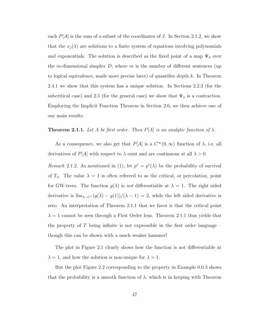
Remark 2.1.2. As mentioned in (1), let p∗ = p∗(λ) be the probability of survival
of Tλ. The value λ = 1 is often referred to as the critical, or percolation, point
for GW-trees. The function g(λ) is not differentiable at λ = 1. The right sided
derivative is limλ→1+(g(λ) − g(1))/(λ − 1) = 2, while the left sided derivative is
zero. An interpretation of Theorem 2.1.1 that we favor is that the critical point
λ = 1 cannot be seen through a First Order lens. Theorem 2.1.1 thus yields that
the property of T being infinite is not expressible in the first order language –
though this can be shown with a much weaker hammer!
The plot in Figure 2.1 clearly shows how the function is not differentiable at
λ = 1, and how the solution is non-unique for λ > 1.
But the plot Figure 2.2 corresponding to the property in Example 0.0.3 shows
that the probability is a smooth function of λ, which is in keeping with Theorem
47
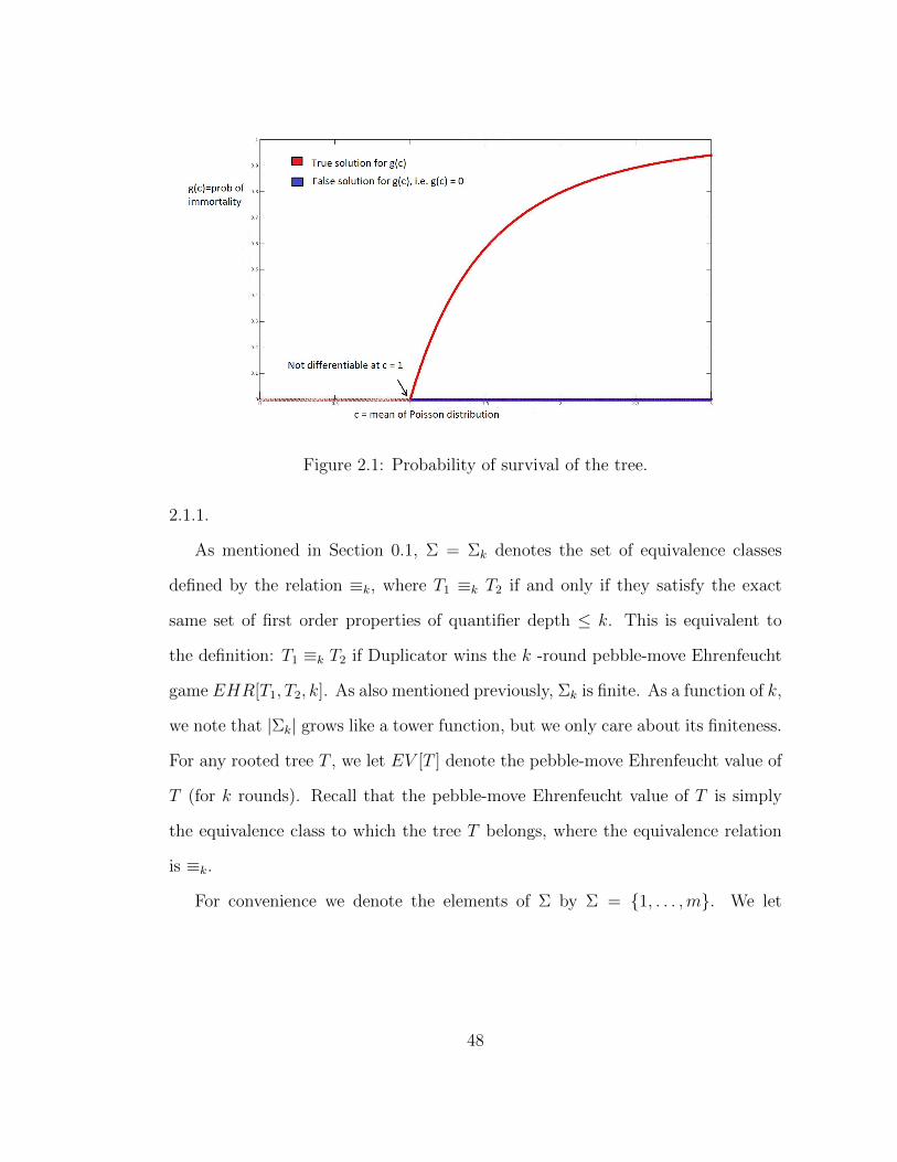
Figure 2.1: Probability of survival of the tree.
2.1.1.
As mentioned in Section 0.1, Σ = Σk denotes the set of equivalence classes
defined by the relation ≡k, where T1 ≡k T2 if and only if they satisfy the exact
same set of first order properties of quantifier depth ≤ k. This is equivalent to
the definition: T1 ≡k T2 if Duplicator wins the k -round pebble-move Ehrenfeucht
game EHR[T1, T2, k]. As also mentioned previously, Σk is finite. As a function of k,
we note that |Σk| grows like a tower function, but we only care about its finiteness.
For any rooted tree T , we let EV [T ] denote the pebble-move Ehrenfeucht value of
T (for k rounds). Recall that the pebble-move Ehrenfeucht value of T is simply
the equivalence class to which the tree T belongs, where the equivalence relation
is ≡k.
For convenience we denote the elements of Σ by Σ = 1, . . . ,m. We let
48
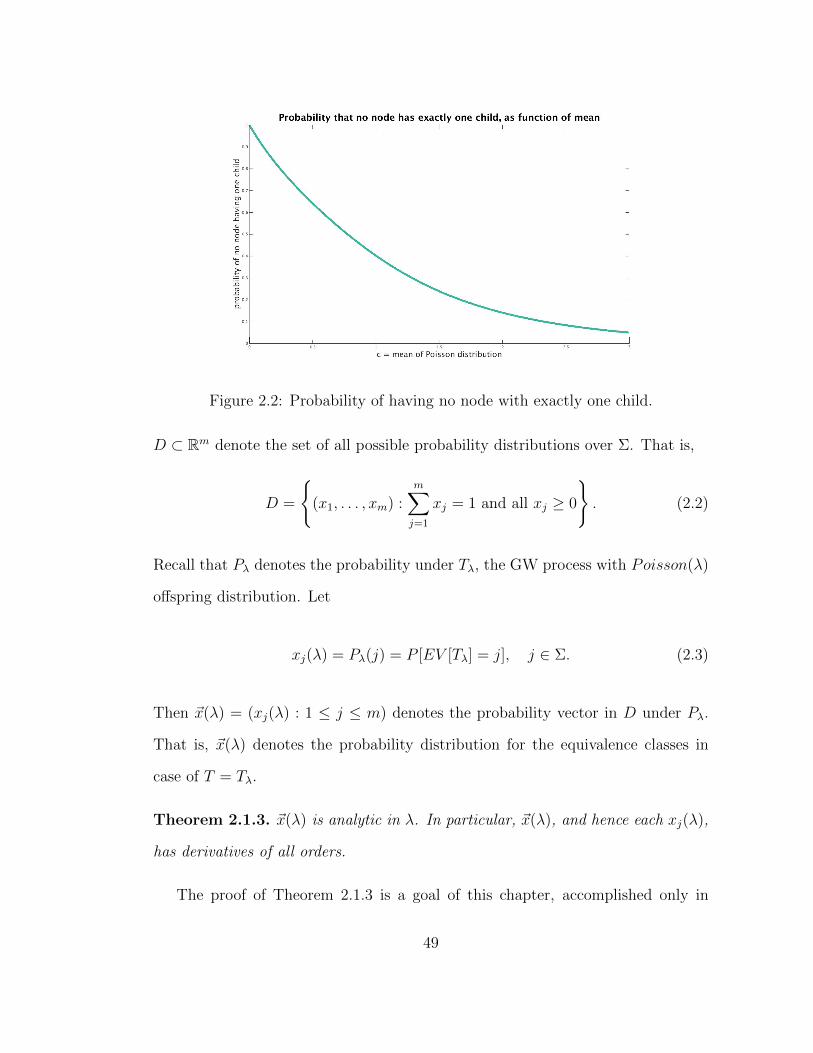
Figure 2.2: Probability of having no node with exactly one child.
D ⊂ Rm denote the set of all possible probability distributions over Σ. That is,
D =
(x1, . . . , xm) :
m∑j=1
xj = 1 and all xj ≥ 0
. (2.2)
Recall that Pλ denotes the probability under Tλ, the GW process with Poisson(λ)
offspring distribution. Let
xj(λ) = Pλ(j) = P [EV [Tλ] = j], j ∈ Σ. (2.3)
Then ~x(λ) = (xj(λ) : 1 ≤ j ≤ m) denotes the probability vector in D under Pλ.
That is, ~x(λ) denotes the probability distribution for the equivalence classes in
case of T = Tλ.
Theorem 2.1.3. ~x(λ) is analytic in λ. In particular, ~x(λ), and hence each xj(λ),
has derivatives of all orders.
The proof of Theorem 2.1.3 is a goal of this chapter, accomplished only in
49
Section 2.6 after many preliminaries. Any first order sentence A of quantifier
depth ≤ k is determined, tautologically, by the set S(A) of those j ∈ Σ such that
all T with EV [T ] = j have property A. For any j ∈ Σ either all T with EV [T ] = j
have property A, or no T with EV [T ] = j hase property A. We may therefore
decompose the Pλ[A] of (2.1) into
Pλ[A] =∑j∈S(A)
xj(λ). (2.4)
Theorem 2.1.1 will therefore follow from Theorem 2.1.3.
2.1.1 Recursive States
The following notion will be made more precise in the sequel: in the k-round
pebble-move Ehrenfeucht game, all counts ≥ k are roughly all “the same.” This
will be made precise in the subsequent Lemma 2.1.4. We define
C = 0, 1, . . . , k − 1, ω. (2.5)
The phrase “there are ω copies” is to be interpreted as “there are ≥ k copies.”
We call v ∈ T a rootchild if its parent is the root R. For w 6= R we say v is
the rootancestor of w if v is that unique rootchild with w ∈ T (v). Of course, a
rootchild is its own rootancestor.
Lemma 2.1.4 roughly states that the pebble-move Ehrenfeucht value of a tree
T is determined by the Ehrenfeucht values EV [T (v)] for all the rootchildren v.
To clarify: ω rootchildren means at least k rootchildren, while i rootchildren,
i ∈ C \ ω, means precisely i rootchildren.
50
Recall that Σ = Σk is the set of all equivalence classes under ≡k., and we are
setting |Σ| = m.
Lemma 2.1.4. Let ~n = (n1, . . . , nm) with all nj ∈ C. Let T have the property that
for all 1 ≤ j ≤ m there are nj rootchildren v with EV [T (v)] = j. Then σ = EV [T ]
is uniquely determined.
Definition 2.1.5. Let
Γ : (n1, . . . , nm) : ni ∈ C for all 1 ≤ i ≤ m → Σ (2.6)
be given by σ = Γ(~n) with ~n, σ satisfying the conditions of Lemma 2.1.4. Then Γ
is called the recursion function.
Proof of Lemma 2.1.4. Let T, T ′ have the same ~n. We give a strategy for the
Duplicator in the Ehrenfeucht game EHR[T, T ′, k]. Duplicator will create a partial
matching between the rootchildren v ∈ T and the rootchildren v′ ∈ T ′. When v, v′
are matched, EV [T (v)] = EV [T ′(v′)]. At the end of any round of the game call
a rootchild v ∈ T (similarly v′ ∈ T ′) free if no w ∈ T (v) (correspondingly no
w′ ∈ T ′(v′)) has yet been selected.
Suppose Spoiler plays w ∈ T (similarly w′ ∈ T ′) with rootancestor v. Suppose
v is free. Duplicator finds a free v′ ∈ T ′ with EV [T (v)] = EV [T ′(v′)]. When
EV [T (v)] = j ∈ Σ and nj 6= ω, then as the number of rootchildren of T with
Ehrenfeucht value j is exactly the same as that in T ′, hence this can be done. In
the special case where nj = ω the vertex v′ may be found as there have been at
most k − 1 rounds prior to this move and so there are at most k − 1 rootchildren
w′ ∈ T ′ with EV [T ′(w′)] = j that are not free. Duplicator then matches v, v′.
Duplicator can win EHR[T (v), T ′(v′), k] as EV [T (v)] = EV [T ′(v′)]. Once v, v′
51
have been matched any move z ∈ T (v) is responded to with a move z′ ∈ T ′(v′),
and vice versa, using the strategy for EHR[T (v), T ′(v′), k].
Remark 2.1.6. Tree automata consist of a finite state space Σ, an integer k ≥ 1, a
map Γ as in (2.6) and a notion of accepted states. While first order sentences yield
tree automata, the notion of tree automata is broader. Tree automata roughly
correspond to second order monadic sentences, especially EMSO’s. See [12] for
more general discussions on this topic.
2.1.2 Solution as Fixed Point
We come now to the central idea. We define, for λ > 0, a map Ψλ : D → D.
Let ~x = (x1, . . . , xm) ∈ D, a probability distribution over Σ. Imagine root R
has Poisson mean λ children. To each child we assign, independently, a j ∈ Σ
with distribution ~x. Let nj ∈ C be the number of children assigned j. Let ~n =
(n1, . . . , nm). Apply the recursion function (equation 2.6) Γ to get σ = Γ(~n). We
then define Ψλ(~x) to be the distribution of this random σ.
The special nature of the Poisson distribution allows a concise expression.
When the initial distribution is ~x, the number of children assigned j will have
a Poisson distribution with mean λxj, and these numbers are mutually indepen-
dent over j ∈ Σ. Thus,
P [nj = u] = e−λxj(λxj)
u
u!for u ∈ C, u 6= ω, (2.7)
and
P [nj = ω] = 1−k−1∑u=0
P [nj = u]. (2.8)
52
From the independence, for any ~a = (a1, . . . , am) with a1, . . . , am ∈ C,
P [~n = ~a] =m∏j=1
P [nj = aj]. (2.9)
Thus, writing Ψλ(x1, . . . , xm) = (y1, . . . , ym),
yj = ΣP [~n = ~a] (2.10)
where the summation is over all ~a with Γ(~a) = j.
We place all Ψλ into a single map ∆:
∆ : D × (0,∞)→ D by ∆(~x, λ) = Ψλ(~x). (2.11)
Setting ∆(x1, . . . , xm, λ) = (y1, . . . , ym), the yj are finite sums of products of poly-
nomials and exponentials in the variables x1, . . . , xm, λ. In particular, all partial
derivatives of all orders exist everywhere.
Recall from (2.3) that ~x(λ) denotes the probability distribution for the equiv-
alence classes under the probability measure Pλ for T = Tλ.
Lemma 2.1.7. Let Ψλ : D → D be as defined in 2.1.2, where D is the set of
all probability distributions on Σ, the set of equivalence classes from the k-round
Ehrenfeucht game in the first order setting, as defined in 0.1.1. Suppose ~x(λ) is a
fixed point for Ψλ : D → D. That is, Ψλ(~x(λ)) = ~x(λ).
53
Proof. By definition of Γ, we know, for any j ∈ Σ,
Ψλ(~x(λ))(j) =∑
~a∈CΣ:Γ(~a)=j
m∏i=1
P [ni = ai|~x = ~x(λ)], from (2.9),
=∑
~a∈CΣ:Γ(~a)=j
m∏i=1
P [Poisson(λ · xi(λ)) = ai]
=∑
~a∈CΣ:Γ(~a)=j
Pλ[~n = ~a]
=Pλ[j] = xj(λ).
Example 2.1.8. For many particular A, the size of Σ, which may be thought of
as the state space, may be reduced considerably. Let A be the property given in
Example 0.0.3, that no node has precisely one child. For every node in a given
tree, we define state 1 which denotes that A is true for the subtree rooted at this
node, and state 2 which denotes that A is false for the subtree rooted at this node.
We set C = 0, 1, ω with ω meaning “at least two.” Let n1, n2 ∈ C be the number
of rootchildren v with T (v) having state 1, 2 respectively. Then T is in state 1
if and only if ~n = (n1, n2) has one of the values (0, 0), (ω, 0). Let D be the set
of distributions on the two states, D = (x, y) : 0 ≤ x ≤ 1, y = 1 − x. Then
Ψλ(x, y) = (z, w) with w = 1− z and
z = e−λxe−λy + e−λy[1− e−λx − (λx)e−λx] = e−λy[1− (λx)e−λx]. (2.12)
The fixed point (x, y) then has x = P [A] satisfying the equation
x = e−λ(1−x)[1− (λx)e−λx]. (2.13)
54
Example 2.1.9. Let A be that there is a vertex v with precisely one child who has
precisely one child. Let state 1 be that A is true. Let state 2 be that A is false but
that the root has precisely one child. Let state 3 be all else. Set C = 0, 1, ω, with
ω meaning ≥ 2. Set D = x, y, z : x + y + z = 1, x ≥ 0, y ≥ 0, z ≥ 0. T is in
state 1 if and only if ~n = (n1, n2, n3) has either n1 6= 0 or n1 = 0, n2 = 1, n3 = 0.
T is in state 2 if and only if ~n = (0, 0, 1). Then ~x(λ) = (x, y, z) must satisfy the
system (noting z = 1− x− y is dependent):
x = (1− e−λx) + e−λx(λye−λy)e−λz = 1− e−λx + λye−λ (2.14)
y = e−λxe−λy(λze−λz) = λze−λ (2.15)
Here x = P [A].
In general, however, P [A] will be the sum (2.4).
2.2 The Contraction formulation
2.2.1 The Total Variation Metric
On D, we let ||x − y||2 denote the usual Euclidean metric, and ||~x − ~y||1 the
L1 distance. We let TV (~x, ~y) denote the total variation distance. With ~x =
(x1, . . . , xm) and ~y = (y1, . . . , ym) this standard metric is given by
TV (~x, ~y) =1
2||~x− ~y||1 =
1
2
m∑j=1
|xj − yj|. (2.16)
Total variation distance between any two probability distributions µ, ν on the
55
same probability space has a natural interpretation in terms of coupling µ and ν.
This is captured in the following standard result:
Theorem 2.2.1. For any two probability distributions µ, ν on a common proba-
bility space, TV (µ, ν) = minP [X 6= Y ] : (X, Y ) any coupling of µ, ν.
The coupling at which this minimum is indeed attained is known as the optimal
coupling. We refer the reader to Chapter 4 of [6] for further reading, especially
Proposition 4.7 for a proof of existence of the optimal coupling.
2.2.2 The Contraction Theorem
Theorem 2.2.2. Fix any arbitrary λ > 0. Let Ψλ : D → D be as defined in
2.1.2, where D is the set of all probability distributions on Σ, the set of equivalence
classes from the k-round pebble-move Ehrenfeucht game, as defined in 0.1.1. Then
there exists a positive integer s and an α < 1 such that for all ~x, ~y ∈ D,
||Ψsλ(~x)−Ψs
λ(~y)||2 ≤ α||~x− ~y||2. (2.17)
The proof of this result is given in several parts over the next few sections.
The subcritical case is considered in Subsection 2.2.3, whereas the proof in the
supercritical regime requires a more delicate analysis, which is given in detail in
Section 2.5.
The map Ψsλ : D → D has a natural interpretation. Let ~x = (x1, . . . , xm) ∈ D.
Generate a random GW tree T = Tλ but stop at generation s (the root is at
generation 0). To each node (there may not be any) v at generation s assign
independently j ∈ Σ from distribution ~x. Now we work up the tree towards the
root. Suppose, formally by induction, that the nodes w at generation i have been
56

assigned some j ∈ Σ. A v at generation i − 1 will then have nj children assigned
j (allowing nj = ω). The value at v, which is now determined by Lemma 2.1.4,
is given by the recursion function Γ(~n) of Definition 2.6. Ψsλ(~x) will then be the
distribution of the Ehrenfeucht value assigned to the root.
Remark 2.2.3. While this work examines first order properties on rooted trees, it
is instructive to consider the non-first order property A that T is infinite. Set C =
0, ω (ω denoting ≥ 1), and let state 1 be that T is infinite, state 2 that it is not.
T is in state 1 if and only if ~n = (ω, 0) or (ω, ω). Then D = (x, 1−x) : 0 ≤ x ≤ 1
and
Ψλ(x, 1− x) = (1− e−λx, e−λx). (2.18)
However, when λ > 1, Ψλ has two fixed points: (0, 1) and the “correct” (p∗(λ), 1−
p∗(λ)). The contraction property (2.17) will not hold. With ε small, 1− e−λε ∼ cε
and so ~x = (0, 1), and ~y = (ε, 1 − ε) become further apart on application of Ψλ,
when λ > 1.
2.2.3 The Subcritical Case
Here we prove Theorem 2.2.2 under the additional assumption that λ < 1. The
proof in this case is considerably simpler. Further, it may shed light on the general
proof.
Theorem 2.2.4. Fix any arbitrary λ < 1. Let Ψλ : D → D be as defined in
2.1.2, where D is the set of all probability distributions on Σ, the set of equivalence
classes from the k-round pebble-move Ehrenfeucht game. Then, for any ~x, ~y ∈ D,
TV (Ψλ(~x),Ψλ(~y)) ≤ λ · TV (~x, ~y). (2.19)
57
Proof. The main idea is to use a suitable coupling of ~x and ~y. First we fix s ∈ N.
We now imagine two pictures. In both pictures, let v have smany children v1, . . . vs.
In the first picture, we assign, mutually independently, labels X1, . . . Xs ∈ Σ to
v1, . . . vs respectively, with Xi ∼ ~x, 1 ≤ i ≤ s. In the second picture, we assign,
again mutually independently, labels Y1, . . . Ys ∈ Σ to v1, . . . vs, with Yi ∼ ~y, 1 ≤
i ≤ s. The pairs (Xi, Yi), 1 ≤ i ≤ s, are mutually independent, but for every i,
(Xi, Yi) is coupled so that
P [Xi 6= Yi] = TV (~x, ~y). (2.20)
Suppose Xv is the label of the root v in the first picture that we get from the
recursion function Γ (from (2.6)), and Yv that in the second picture. Then Xv ∼
Ψλ(~x), Yv ∼ Ψλ(~y).
TV (Ψλ(~x),Ψλ(~y)) ≤ P [Xv 6= Yv]
≤∞∑s=0
P [Poisson(λ) = s]s∑i=1
P [Xi 6= Yi]
=∞∑s=0
P [Poisson(λ) = s] · s · TV (~x, ~y)
=λ · TV (~x, ~y).
Lemma 2.2.5. Fix any λ < 1. Let Ψλ : D → D be as defined in 2.1.2, where D
is the set of all probability distributions on Σ, the set of equivalence classes from
the k-round pebble-move Ehrenfeucht game. Then Theorem 2.2.2 holds.
58
Proof. The inequalities
||~z||1 ≥ ||~z||2 ≥ m−1/2||~z||1 (2.21)
bound the L1 and L2 norms on Rm by multiples of each other. As TV (~x, ~y) =
12||~x− ~y||1,
TV (~x, ~y) ≥ 1
2||~x− ~y||2 ≥ m−1/2 · TV (~x, ~y). (2.22)
Applying Theorem 2.2.4 repeatedly,
TV (Ψsλ(~x),Ψs
λ(~y)) ≤ λs · TV (~x, ~y). (2.23)
Combining (2.22 and 2.23)
||Ψsλ(~x)−Ψs
λ(~y)||2 ≤ 2 · TV (Ψsλ(~x),Ψs
λ(~y)) ≤ 2λs · TV (~x, ~y) ≤ 2λs√m ||~x− ~y||2.
(2.24)
We select s so that 2λs√m < 1 and set α = 2λs
√m.
2.3 Universality
We define a function Rad[i] on the nonnegative integers by the recursion
Rad[0] = 0 and Rad[i+ 1] = 3Rad[i] + 1 for i ≥ 0. (2.25)
Recall from Chapter 1 that ρ(v, w) is the usual graph distance between any two
nodes v and w in a given tree T . As in Chapter 1, we consider, for r a nonnegative
integer and v ∈ V (T ), the ball B(v, r) of radius r around v, with v a designated
59

vertex of B(v, r).
We can define an equivalence relation, depending on k, on such balls. This is
somewhat more general and less restrictive a definition than the equivalence ≡M ;k
we discuss in Chapter 1. Although Section 2.3 largely derives from Chapter 1, we
retain it here because of this reason, and its relevance in Section 2.5. Moreover,
(2.25) gives a more concise formula for the radius Rad[k] of the neighbourhood
around the root we need to consider, to conclude about all first order properties
of quantifier depth ≤ k.
As in Section 0.1, we define B(v, r) ≡k B(v′, r) if the two balls satisfy the same
first order sentences of quantifier depth at most k − 1, with v, v′ as designated
vertices, allowing the relations π and =. Equivalently, B(v, r) ≡k B(v′, r) if Du-
plicator wins the k-round pebble-move Ehrenfeucht game on these sets in which
the 0-th round is mandated to be the pair (v, v′) and Duplicator must preserve the
relations π and =. Let ΣBALLk denote the set of all equivalence classes under the
equivalence relation ≡k, on all such balls with designated vertices inside trees.
Definition 2.3.1. We say S1, S2 ⊂ T are strongly disjoint if there are no v1 ∈ S1,
v2 ∈ S2 with ρ(v1, v2) ≤ 1.
Definition 2.3.2. We say T is k-full if for any v1, . . . , vk−1 ∈ T and any σ ∈ ΣBALLk
there exists a vertex v such that
i. B(v,Rad[k − 1]) is in equivalence class σ.
ii. B(v,Rad[k − 1]) is strongly disjoint from all B(vi, Rad[k − 1]).
iii. B(v,Rad[k − 1]) is strongly disjoint from B(R,Rad[k]), R the root.
60

Definition 2.3.3. Fix a positive integer k. Consider two trees T and T ′, and two
subsets of vertices C in T and C ′ in T ′. Let the induced subgraphs on C and C ′
both be connected. Suppose we are also given nodes z1, . . . zw in C and z′1, . . . z′w
in C ′ for some 1 ≤ w ≤ k. We say that C and C ′ are k-equivalent if the Duplicator
can win the k-move Ehrenfeucht game on it, maintaining = and π, where zi and
z′i, 1 ≤ i ≤ w, are designated vertices.
Remark 2.3.4. Note that the k-move Ehrenfeucht game with designated vertices
z1, . . . , zw ∈ T , z1 . . . , z′w ∈ T is equivalent to the k + w-move Ehrenfeucht game
in which the first w moves are mandated to be zi ∈ T, z′i ∈ T ′
When T is k-full our next result shows that the truth value of first order
sentences of quantifier depth at most k is determined by examining T “near” the
root. This “inside-outside” strategy is well known, see, for example, [5].
Theorem 2.3.5. Let T, T ′ with roots R,R′ both be k-full. Suppose
B(R,Rad[k]) ≡k+1 B(R′, Rad[k]). Then T, T ′ have the same (k round) pebble-
move Ehrenfeucht value.
Proof. Let T, T ′ satisfy the conditions of Theorem 2.3.5. We give a strategy for
Duplicator to win the k-move Ehrenfeucht game. For convenience we add a round
zero in which the roots R,R′ are selected. Duplicator will insure inductively that
with i moves remaining the following somewhat complicated condition, denoted as
OK[i], holds:
Let x0, x1, . . . , xk−i ∈ T , y0, y1 . . . , yk−i ∈ T ′, where x0 and y0 are the roots of T
and T ′ respectively. Let Si denote the union of the balls B(xj, Rad[i]), 0 ≤ j ≤ k−i
and let S ′i denote the union of the balls B(yj, Rad[i]), 0 ≤ j ≤ k − i. The set Si
splits T and the set S ′i splits T ′ into components. Duplicator wants to ensure
61
that for every such component C in T and the corresponding component C ′ in
T ′, if xj ∈ C then yj ∈ C ′ and vice versa; also, C and C ′ should be equivalent
components in the sense of Definition 2.3.3, with exactly those xj (correspondingly
yj), 0 ≤ j ≤ k − i, as designated vertices that are in C (correspondingly C ′).
When i = k, OK[k] holds because x0 = R, y0 = R′ and by the hypothesis of
Theorem 2.3.5, B(R,Rad[k]) ≡k+1 B(R′, Rad[k]).
Now suppose, by induction, that k ≥ i > 0 and x0, x1, . . . , xk−i ∈ T ,
y0, y1 . . . , yk−i ∈ T ′ satisfy OK[i], with x0 the root of T and y0 that of T ′. In the
next round suppose (the other case being identical) Spoiler selects xk−i+1 ∈ T .
Now there are two possible cases:
i. Inside case: There exists xj with 0 ≤ j ≤ k − i, such that
ρ (xj, xk−i+1) ≤ 2Rad[i − 1] + 1. Then the ball B (xk−i+1, Rad[i− 1])
is entirely contained in B (xj, Rad[i]), from the recursion (2.25)). So, we can
choose the corresponding v in B (yj, Rad[i]) which allows him to win the game
on the components containing B (xj, Rad[i]) , B (yj, Rad[i]), of k rounds.
By induction hypothesis, the components formed by⋃k−il=0 B (xl, Rad[i])
are equivalent; the balls B (xk−i+1, Rad[i− 1]) and B (yk−i+1, Rad[i− 1])
are contained in the balls B (xj, Rad[i]) and B (yj, Rad[i]) respectively.
Consequently, the components formed by⋃k−i+1l=0 B (xl, Rad[i− 1]) will also
be equivalent.
ii. Outside case: Suppose xk−i+1 is chosen such that ρ (xj, xk−i+1) > 2Rad[i −
1] + 1 for all 0 ≤ j ≤ k− i. Using the definition of k-full as in 2.3.2, we know
62
that there exists v ∈ T ′ such that B (v,Rad[k − 1]) is strongly disjoint from
B (yj, Rad[k − 1]) for all 1 ≤ j ≤ k− i, and from B (R′, Rad[k − 1]); further,
B (v,Rad[k − 1]) ≡k B (xk−i+1, Rad[k − 1]). Duplicator chooses yk−i+1 = v.
Then observe that for every 0 ≤ j ≤ k − i, B (xj, Rad[i− 1]) (correspond-
ingly B (yj, Rad[i− 1])) is strongly disjoint from B (xk−i+1, Rad[i− 1])
(correspondingly B (yk−i+1, Rad[i− 1]), and thus in the component⋃k−il=0 B (xl, Rad[i− 1])
c(correspondingly
⋃k−il=0 B (yl, Rad[i− 1])
c);
further B (yk−i+1, Rad[k − 1]) ≡k B (xk−i+1, Rad[k − 1]).
So, regardless of Spoiler’s choice of xk−i+1 ∈ T , Duplicator has selected yk−i+1 ∈
T ′ and OK[i− 1] is satisfied.
Thus Duplicator can play the entire k rounds so that at the end of the game
OK[0] holds. But the union of the balls of radius zero around the vertices selected
are equivalent in T, T ′. Hence Duplicator has won!
Definition 2.3.6. We replace the complex notion of k-full by a simpler sufficient
condition. For each σ ∈ ΣBALLk create k copies of a ball in that class. Take a
root vertex v and on it place k · |ΣBALLk | disjoint paths (parent to child) of length
Rad[k] + Rad[k − 1] + 1. Identify each endpoint with the roof of one of these
copies. We let UNIVk denote this tree, which we can picture, rather fancifully, as
a Christmas tree.
Definition 2.3.7. T is called s-universal (given a fixed positive integer k) if all T ′
with T |s ∼= T ′|s have the same k-Ehrenfeucht value. Thus EV [T ] is determined by
T |s completely.
63

Theorem 2.3.8. If for some v, T (v) ∼= UNIVk then T is k-full. Thus, by Theorem
2.3.5, the k-Ehrenfeucht value of T is determined by B(R,Rad[k]) or T |Rad[k]. In
other words, T is Rad[k]-universal.
Remark 2.3.9. Many other trees could be used in place of UNIVk, we use this
particular one only for specificity.
Remark 2.3.10. A subtree T (v), where v is not the root, cannot determine the
Ehrenfeucht value of T as, for example, it cannot tell us if the root has, say, pre-
cisely two children. Containing this universal tree UNIVk tells us everything about
the Ehrenfeucht value of T except properties relating to the local neighborhood of
the root.
Recall from Subsection 1.1.1 the definition of rapidly determined properties
in the context of Galton-Watson trees. It is particularly instructive to note that
many non-first order properties are not rapidly determined, as illustrated in the
remark below.
Remark 2.3.11. Consider the property that Tλ is infinite (where of course we con-
sider λ > 1). Given X1, . . . , Xs of the fictitous continuation, if the tree has stopped
then we know it is finite. Suppose, however, (as holds with positive limiting prob-
ability) after X1, . . . Xs the tree is continuing to grow. If at that stage there are
many nodes we can be reasonably certain that T will be infinite, but we cannot
be tautologically sure. This property is not rapidly determined.
Remark 2.3.12. In this work, we restrict the language in which A is expressed.
It has been suggested that another approach would be to restrict A to rapidly
determined properties.
The following few results are recalled from Chapter 1, but are relevant for the
64
subsections that follow.
Lemma 2.3.13. Let T0 be an arbitrary finite tree. Let A be the (non first order)
property that either the process has aborted by time s or there exists v ∈ T with
T (v) ∼= T0. Then A is rapidly determined in parameter s.
The proof is given in Theorem 1.1.3 of Chapter 1. Let T0 have depth d. Roughly
speaking, when we examine X1, . . . , Xs either the process has aborted or it has
not. If not, quite surely some i ≤ sε has T (i) ∼= T0. Here ε is chosen small enough
(dependent on λ, d) so that quite surely the descendants of all i ≤ sε, down to d
generations, have indices ≤ s.
Lemma 2.3.14. Every first order property A is rapidly determined.
Proof. Let A have quantifier depth k. Let T0 be the universal tree UNIVk as given
by Definition 2.3.6. From Lemma 2.3.13 if T has not aborted by time s then quite
surely some T (i) ∼= T0. But then T is already k-full and already has depth at least
Rad[k]. By Theorem 2.3.5, the k-Ehrenfeucht value of T , hence the truth value of
A, is determined solely by T |Rad[k], and hence tautologically by X1, . . . Xs.
Lemma 2.3.15. Fix a positive integer k. Then quite surely (in s), Tλ is s-
universal.
Proof. Lemma 2.3.14 gives that the k-Ehrenfeucht value of T is quite surely de-
termined by X1, . . . , Xs. When this is so it is tautologically determined by T |s,
which has more information.
65
2.4 Unique fixed point
Theorem 2.4.1. Let Ψλ : D → D be as defined in 2.1.2, where D is the set of
all probability distributions on Σ, the set of equivalence classes from the k-round
Ehrenfeucht game in the first order setting, as defined in 0.1.1. Then Ψλ has a
unique fixed point.
Proof. Let f(s) be the probability that Tλ is not s-universal. For any ~y, ~z ∈ D we
couple Ψsλ(~y),Ψs
λ(~z). Generate Tλ down to generation s and then give each node
at generation s a σ ∈ Σ, mutually independently, with marginal distribution ~y,
respectively ~z. Then Ψsλ(~y), Ψs
λ(~z) will be the distributions of the induced states of
the root. But when Tλ is s-universal this will be the same for any ~y and ~z. Hence
TV [Ψsλ(~y),Ψs
λ(~z)] ≤ f(s). When ~y, ~z are fixed points of Ψ, TV [~y, ~z] ≤ f(s). As
f(s)→ 0, ~y = ~z.
Remark 2.4.2. Theorem 2.4.1 will also follow from the more powerful Theorem
2.2.2.
Remark 2.4.3. It is a challenging exercise to show directly that the solution x to
(2.13) or the solution x, y to the system (2.14 and 2.15) are unique.
2.5 A proof of contraction
2.5.1 A Two Stage Process
Here we prove Theorem 2.2.2 for arbitrary λ. Let D0 be the depth of UNIVk,
as given by Definition 2.3.6. We shall set
s = s0 +D0 with s0 ≥ 2 ·Rad[k] (2.26)
66
and think of T |s as being generated in two stages. In Stage 1 we generate T |s0 .
From Lemma 2.3.15, by taking s0 large, this will be s0-universal with probability
near one. In Stage 2 we begin with an arbitrary but fixed T0 of depth at most
s0. (We say “at most” because it includes the possibility that T0 has no vertices
at depth s0.) From each node at depth s0, mutually independently, we generate
a GW-tree down to depth D0. We denote by Ext(T0) this random tree, now of
depth (at most) s.
Definition 2.5.1. For any T0 of depth at most s0, BAD[T0] is the event that
Ext(T0) is not s0-universal.
Lemma 2.5.2. There exists positive β such that for any T0 of depth at most s0
P (BAD[T0]) ≤ e−tβ (2.27)
where t denotes the number of nodes of T0 at depth s0.
Proof. Let v1, . . . , vt denote the nodes of T0 at generation s0. Each of them
independently generates a GW tree. Let 1 − e−β denote the probability that
T (vi) ∼= UNIVk. With probability e−tβ no T (vi) ∼= UNIVk. But otherwise Ext(T0)
is s0-universal.
2.5.2 Splitting the Extension
Let T0 be an arbitrary tree of depth s0. Let ~x ∈ D. Assign to the depth
s nodes of Ext(T0) independent identically distributed labels j ∈ Σ taken from
distribution ~x. Applying the recursion function Γ of Definition 2.1.5 repeatedly up
the generations yields a unique Ehrenfeucht value for the root R.
67
Definition 2.5.3. Let Ψsλ(T0, ~x) denote the induced distribution of the Ehren-
feucht value for the root R as derived in the description above.
Lemma 2.5.4. Let Ψλ : D → D be as defined in 2.1.2, where D is the set of
all probability distributions on Σ, the set of equivalence classes from the k-round
Ehrenfeucht game in the first order setting, as defined in 0.1.1. Then,
TV (Ψsλ(~x),Ψs
λ(~y)) ≤∑
P (T |s0 ∼= T0) · TV (Ψsλ(T0, ~x),Ψs
λ(T0, ~y)) (2.28)
where the sum is over all T0 of depth (at most) s0.
Proof. We split the distribution of T into the distribution of Ext(T0), with prob-
ability P [T |s0 ∼= T0], over each T0 of depth (at most) s0.
2.5.3 Some Technical Lemmas
Let X = X(λ, s) be the number of descendants at generation s of the GW tree
T = Tλ. Let Y be the sum of t independent copies of X. The next result (not the
best possible) is that the tail of Y is bounded by exponential decay in t.
Lemma 2.5.5. There exists β > 0 and y0 such that for y ≥ y0
P [Y ≥ yt] ≤ e−ytβ. (2.29)
Proof. Set f(c) = ln[E[ecX ]]. We employ Chernoff bounds sub-optimally, taking
simply c = 1. (We require here a standard argument that E[eX ] is finite.) Then
E[eY ] = et·f(1) and
P [Y ≥ yt] ≤ E[eY ]e−yt ≤ e(f(1)−y)t. (2.30)
68
For y ≥ 2f(1), f(1)− y ≤ −y/2 and we may take β = 12.
Lemma 2.5.6. Let K, γ > 0. Let BAD be an event with P [BAD] ≤ Ke−tγ.
Then, for positive constants k, κ,
E[Y · 1BAD] ≤ kte−tκ, (2.31)
where Y is as defined above.
Remark 2.5.7. The idea is that, in the worst case, the event BAD would coincide
with the event Y ≥ s where P [Y ≥ s] = Ke−tγ, for some s > 0. But as seen in
the following proof, in this situation too, E[Y 1BAD] can be bounded as in (2.31).
Proof of Lemma 2.5.6. We split Y into Y < y1t and Y ≥ y1t, where y1 needs
to be chosen suitably.
E[Y 1BAD] = E[Y 1BAD 1Y <y1t] + E[Y 1BAD 1Y≥y1t], (2.32)
where the first term is bounded by y1tP [BAD] ≤ Ky1te−tγ. The second term is
bounded above by E[Y 1Y≥y1t], which we bound using Chernoff type arguments.
First, recall that Y is the sum of t i.i.d. copies ofX = X(λ, s) which is the number of
nodes at generation s of Tλ. Suppose ϕs denotes the cumulant-generating function
of X, defined as
ϕs(c) = logE[ecX ]. (2.33)
We fix some c > 1 and choose
y1 = max
y0,
γ + ϕs(c)
c
, (2.34)
69
where γ is as in the bound of P [BAD], and y0 as in Lemma 2.5.5. From (2.29)
and (2.34), we then have
E[Y 1Y≥y1t] ≤y1tP [Y ≥ y1t] +∞∑
k=by1tc+1
P [Y ≥ k]
≤y1te−y1tβ + E
[ecY] ∫ ∞by1tc
e−cxdx
=y1te−y1tβ + eϕs(c)t
1
ce−cby1tc
≤y1te−y1tβ + eϕs(c)t
ec
ce−cy1t
≤y1te−y1tβ +
ec
ce−γt.
The desired bound now follows easily, by choosing κ = min y1β, γ and k =
Ky1 + y1 + ec/c.
2.5.4 Bounding Expansion
Lemma 2.5.8. There exists K0 (dependent only on s0, k) such that for any T0 and
any ~x, ~y ∈ D
TV (Ψsλ(T0, ~x),Ψs
λ(T0, ~y)) ≤ K0 · TV (~x, ~y), (2.35)
where Ψsλ(T0, ~x) is as defined in Definition 2.5.3.
Remark 2.5.9. As K0 may be large, Lemma 2.5.8, by itself, does not give a con-
tracting mapping. It does limit how expanding Ψsλ(T0, ·) can be.
Remark 2.5.10. Let t be the number of nodes of T0 at depth s0. The expected
number of nodes in Ext(T0) at level s = s0 + D0 is then tK1 with K1 = λD0 .
The methods of Theorem 2.2.4 would then give Lemma 2.5.8 with K0 = K1t.
70
However, when λ > 1 this K0 would be unbounded in t. Our concern is then with
large t, though technically, the proof below works for all t.
Proof. Let t be the number of nodes of T0 at depth s0. Let TV (~x, ~y) = ε. We again
couple ~x, ~y. As before, let Y be the number of nodes in Ext(T0) at level s. Given
Y = y, let us name these nodes u1, . . . uy. Again we create two pictures. In the
first picture, we assign, mutually independently, labels Xi ∈ Σ to ui, with Xi ∼ ~x,
and in the second picture, label Zi ∼ ~y. (Xi, Zi), 1 ≤ i ≤ y mutually independent,
but Xi, Zi are coupled so that
P [Xi 6= Zi] = TV (~x, ~y) = ε. (2.36)
The probability of the event that for at least one i, Xi 6= Zi is then bounded above
by y · ε.
Suppose X ∈ Σ is the label of the root of Ext(T0) in the first picture, and Z
that in the second picture, determined by using the recursion function Γ repeatedly
upward starting at level s. Then X ∼ Ψsλ(T0, ~x), Z ∼ Ψs
λ(T0, ~y), from Definition
2.5.3.
Recall, from Definition 2.5.1, that BAD[T0] is the event that Ext(T0) is not
s0-universal. If GOOD[T0] = BAD[T0]c, then under GOOD[T0], the Ehrenfeucht
value of Ext(T0) is completely determined by Ext(T0)|s0 , which is T0 itself. And
71
as T0 is fixed, this means that EV [Ext(T0)] is then independent of ~x, ~y. Thus
TV (Ψsλ(T0, ~x),Ψs
λ(T0, ~y)) ≤ P [X 6= Z]
≤∞∑y=0
P [Y = y] · y · ε · 1BAD[T0]
=E[Y · 1BAD[T0]]ε.
From Lemma 2.5.2 and Lemma 2.5.6,
TV (Ψsλ(T0, ~x),Ψs
λ(T0, ~y)) ≤ A(t)ε with A(t) = kte−tκ. (2.37)
Here A = A(t) approaches zero as t→∞ and so there exists K0 such that A ≤ K0
for any choice of t.
2.5.5 Proving Contraction
We first show Theorem 2.2.2 in terms of the TV metric. Pick s0 sufficiently large
so that, say, the probability that T |s0 is not s0-universal is at most (2K0)−1, K0
given by Lemma 2.5.8. This can be done because of Lemma 2.3.15. Let ~x, ~y ∈ D
with ε = TV (~x, ~y). We bound TV (Ψsλ(~x),Ψs
λ(~y)) by Lemma 2.5.4. Consider
TV (Ψsλ(T0, ~x),Ψs
λ(T0, ~y)). When T0 is s0-universal this has value zero. Otherwise
its value is bounded by K0ε by Lemma 2.5.8. Lemma 2.5.4 then gives
TV (Ψsλ(~x),Ψs
λ(~y)) ≤ 1
2K0
K0ε ≤ε
2. (2.38)
Finally, we switch to the L2 metric. For B a sufficiently large constant the
72

inequalities (2.21) yield, say,
||ΨsBλ (~x)−ΨsB
λ (~y)||2 ≤1
2||~x− ~y||2. (2.39)
Then Theorem 2.2.2 is satisfied with s replaced by sB and α = 12.
2.6 Implicit function
Here we deduce Theorem 2.1.3 and hence Theorem 2.1.1, that P [A] is always
an analytic function of λ. This follows from three results:
i. The function ∆(λ, ~x) = Ψλ(~x) has all derivatives of all orders.
ii. For each λ > 0 the function
F (~x) = Ψλ(~x)− ~x (2.40)
has a unique zero ~x = ~x(λ).
iii. The function Ψλ : D → D is contracting in the sense of Theorem 2.2.2.
(i) is discussed in Subsection 2.1.2, where we first define Ψλ (~x), whereas (ii)
is addressed in Theorem 2.4.1. The proof of (iii) can be found in two parts: the
subcritical case in Subsection 2.2.3, and the supercritical case in Section 2.5.
Let J be the Jacobian matrix of Ψλ at ~x(λ). From Property (iii) all of the
eigenvalues of J lie inside the complex unit circle. Then J − I is the Jacobian of
F from Property (ii). Then (J − I)−1 = −∑∞u=0 Ju is a convergent sequence, and
so J − I is invertible. As by Property (i), the function ∆ is smooth, the analytic
73
version of the Implicit Function Theorem gives that the fixed point function ~x(λ)
of F is analytic in λ, and hence also C∞.
74
Chapter 3
Finiteness is not almost surely an
EMSO
3.1 Introduction and outline of the chapter
There are two main parts to Chapter 3. As mentioned in the introduction, we
investigate if finiteness of rooted trees is expressible as an EMSO or not. The first,
immediate question to ask is one that involves no probability: if tautologically,
there exists some EMSO which coincides with finiteness, i.e. if there is an EMSO
(of an arbitrary, but fixed a priori, quantifier depth k) which is satisfied precisely
by the set of finite trees alone. In Theorem 3.1.1, we show that indeed this is not
possible.
But the other, and perhaps more significant, goal of Chapter 3 is to answer
the following question that is more interesting to probabilists: is it possible that
under the measure Pλ induced by the Poisson(λ) Galton-Watson branching process,
finiteness of the tree is expressible as an EMSO on all but a subset of trees of
75
measure 0? We answer this question in the negative, in Theorem 3.1.2.
Theorem 3.1.1. Fix a positive integer k. We can construct a finite tree T1 and an
infinite tree T2, both deterministic, such that Duplicator wins EHR[T1, T2,Σ, k].
Theorem 3.1.2. Fix a positive integer k. We can construct a finite tree T1 (de-
terministic) and a family T2 of infinite trees, such that Pλ(T2) > 0, and for every
T2 ∈ T2, Duplicator wins EHR[T1, T2,Σ, k].
As we shall see in the subsequent sections of this chapter, we give an almost
explicit construction of T1. The trees in the family T2 are closely connected with
T1. We shall consider, in some sense, a Christmas tree like structure, just as we
did while constructing the universal tree UNIVk in Theorem 1.3.3. We have a
family of finite trees (which we define explicitly in Section 3.5. We consider a
long path starting at the root, and the vertex at the end of the path has several
children, and sufficient number of copies of each tree from this family hanging from
these children. This roughly describes the structure of T1. Every tree T2 of the
family T2 has the following structure: we start with the same finite tree as T1, but
additionally, the last vertex of the long path starting at the root has a child with
a GW tree, conditioned on survival, coming out of it. Obviously, this guarantees,
when λ > 1, that Pλ[T2] > 0.
Both the tautological version and the not-almost-sure version are proved via the
set-pebble Ehrenfeucht games and the types games, which we define in Subsection
3.2. Before we go into the definitions of the games, we need to define rooted
colourings. Let us mention that rooted colourings are simply those colourings of
the nodes of a tree, where the root gets a unique colour. This notion is really quite
simple, but comes in handy later on, since in all our considerations, the roots are
76
special nodes, and assigning them a unique colour helps to readily identify them
as such.
We introduce the types game in Definition 3.2.4. This game is, in a certain
sense, stronger than the set-pebble Ehrenfeucht game. The proofs of both The-
orems 3.1.1 and 3.1.2 happen in two steps. In Section 3.4, we show that, given
two trees T1, T2 which satisfy certain assumptions on the neighbourhoods of their
roots, if Duplicator wins the types game with suitable parameters on T1, T2, then
she also wins the set-pebble Ehrenfeucht game with related parameters. This is
formally stated and proved in Theorem 3.4.1. The conclusion of this theorem gets
used in the proofs of both Theorems 3.1.1 and 3.1.2.
The second parts of the proofs of Theorems 3.1.1 and 3.1.2 differ slightly.
Whereas Theorem 3.1.1 uses Theorem 3.5.2, Theorem 3.1.2 makes use of The-
orem 3.5.6. These two theorems are the two main theorems of Section 3.5. In
Theorem 3.5.2 we show that the Duplicator is able to win the types game on
two given (deterministic) trees T1, T2, where T1 is finite and T2 infinite. Crucially,
Pλ(T2) = 0. In Theorem 3.5.6, we construct a deterministic finite tree T1, and a
family T2 of infinite trees, with Pλ(T2) > 0, such that for every T2 ∈ T2, Duplicator
wins the types game on T1, T2.
3.2 The description of the games
3.2.1 Rooted colourings, set-pebble Ehrenfeucht games
We fix an arbitrary positive integer r and consider a set Σ = col0, . . . colr of
(r+ 1) colours. Later on, we shall consider a set Σen of “augmented” colours that
is derived from Σ. All the definitions / results mentioned about Σ carry over in a
77
natural way to Σen . Henceforth Σ denotes the above set of colours, except for in
Section 3.5, where it can denote any general finite set of colours.
Definition 3.2.1 (Rooted colouring). Given the set Σ of colours, and a tree T ∈ T ,
we call a colouring σ : V (T )→ Σ a (Σ, col0) rooted colouring of T if σ(v) = col0 ⇔
v = RT , for all v ∈ V (T ).
We insist upon assigning a unique colour to the root, because it is a constant
symbol in our language. Given a T ∈ T and a (Σ, col0) rooted colouring σ of T ,
we shall talk of the pair (T, σ) in the subsequent exposition, and call it a (Σ, col0)
coloured tree.
As previously mentioned, the set-pebble Ehrenfeucht game, defined below, will
be our main tool in proving that indeed, there is a set of trees of positive measure
on which finiteness is not an EMSO. We note here that in both the set-pebble
Ehrenfeucht game and the distance preserving Ehrenfeucht game (described in
Definition 3.3.3), we always follow the convention of setting
x0 = RT1 and y0 = RT2 . (3.1)
The winning conditions (EHR 1) through (EHR 3) in Definition 3.2.2, as well as
(DEHR 1) through (DEHR 4) in Definition 3.3.3, are described with this conven-
tion in mind. This convention is once again motivated by the fact that the roots
are constant symbols in our EMSO language.
Definition 3.2.2 (The set-pebble Ehrenfeucht game). This game is played be-
tween two players, the Spoiler and the Duplicator. They are given two trees T1, T2
and a positive integer k. The game consists of (k + 1) rounds, and each round
78
consists of a move by the Spoiler and a move by the Duplicator. These rounds can
be divided into the following:
i. Set round: In this round, called the set round, the Spoiler assigns a (Σ, col0)
rooted colouring σ1 to T1. In reply, Duplicator assigns a (Σ, col0) rooted
colouring σ2 to T2.
ii. Pebble rounds: The subsequent rounds, numbered 1 through k, are called
pebble rounds. In each of these rounds, Spoiler chooses either of the two
trees T1 and T2 and selects a node from that tree. In reply, Duplicator has
to select a node from the other tree.
Suppose xi is the node selected from V (T1), and yi the node selected from
V (T2), in round i, for 1 ≤ i ≤ k. Then Duplicator wins this game, denoted
EHR [T1, T2,Σ, k], if she can maintain all of the following conditions: for all
i, j ∈ [k] (with convention (3.1)),
(EHR 1) π(xj) = xi ⇔ π(yj) = yi;
(EHR 2) σ1(xi) = σ2(yi);
(EHR 3) xi = xj ⇔ yi = yj.
3.2.2 Types and types games
The definition of the types game requires us to first define a type. A type is
defined in terms of Σ, a count k ∈ N, and depth m ∈ N. These same parameters
are also required when we define the types game.
79
Definition 3.2.3 (Type). Given a (Σ, col0) coloured tree (T, σ), we define the
(Σ,m, k)-type of any v ∈ V (T ) recursively on m, as follows. The (Σ, 0, k)-type of
v with respect to (T, σ), denoted TypeΣ,0,k,(T,σ)(v), is simply the colour σ(v) of v.
Suppose we have defined TypeΣ,m−1,k,(T,σ)(v) for all v ∈ V (T ). Let ΓΣ,m−1,k
denote the set of all possible (Σ,m− 1, k) types. For any v ∈ V (T ), if nγ denotes
the number of children u of v with TypeΣ,m−1,k,(T,σ)(u) = γ, we let ~n = (nγ ∧ k :
γ ∈ ΓΣ,m−1,k). The (Σ,m, k)-type of v with respect to (T, σ) is then given by
TypeΣ,m,k,(T,σ)(v) = (σ(v), ~n). (3.2)
Definition 3.2.4 (Types game). This is a single round game played between the
Spoiler and the Duplicator. Given two trees T1 and T2, Spoiler assigns a (Σ, col0)
rooted colouring σ1 to T1. In reply, Duplicator assigns a (Σ, col0) rooted colouring
σ2 to T2. Let n(1)γ be the number of nodes u ∈ V (T1) such that TypeΣ,m,k,(T1,σ1)(u) =
γ, and let n(2)γ be the number of nodes v ∈ V (T2) such that TypeΣ,m,k,(T2,σ2)(v) = γ,
for γ ∈ ΓΣ,m,k. Duplicator wins this game, denoted Type[T1, T2,Σ, k,m], if
n(1)γ ∧ k = n(2)
γ ∧ k for all γ ∈ ΓΣ,m,k. (3.3)
3.3 Further notions required for the proof that
types game is stronger than set-pebble
Ehrenfeucht
In this section, we have several different tools to introduce and discuss, so as to
use them in the proof of Theorem 3.4.1 in Section 3.4. These are done in separate
80
subsections. In Subsection 3.3.1, we introduce the notion of enhanced colouring,
which lets Duplicator attach an extra label to each node of a (Σ, col0) coloured
tree. This additional information helps her choose a judicious colouring in the set
round. In Subsection 3.3.2, we introduce yet another version of the Ehrenfeucht
games, called the distance preserving Ehrenfeucht game (DEHR). The DEHR is
different from the set-pebble Ehrenfeucht game in that it does not involve a set
round, as the trees provided are already coloured. Moreover, the Duplicator needs
to maintain the graph distances between corresponding pairs of chosen vertices
on the two trees (i.e. the language now also involves the relation ρ, which is the
shortest edge distance between two vertices in a graph).
3.3.1 Enhanced colouring and related discussions:
Given a colouring of the vertices of a tree T using the colours in Σ, we discuss
here a method of “refining” this colouring by attaching a second marker to each
node. This enhanced colouring will be of use to the Duplicator in her winning
strategy for Theorem 3.4.1.
Definition 3.3.1. Fix positive integers D,D0, with D even, and D0 +1 many new
colours col′0, . . . col′D0
which are different from all the colours of Σ. Suppose we are
given a (Σ, col0) coloured tree (T, σ). Let
Σen =
(coli, col′j) : 0 ≤ i ≤ r, 0 ≤ j ≤ D0
⋃(coli, j) : 0 ≤ i ≤ r,−D/2 + 1 ≤ j ≤ D/2 . (3.4)
Further define the function F : N ∪ 0 → col′0, . . . col′D0 ∪ −D/2 + 1, . . . D/2
81
as
F (i) =
col′i if 0 ≤ i ≤ D0,
i mod D if i > D0.
(3.5)
Then we define the enhanced colouring corresponding to σ, with respect to the
parameters col′0, . . . col′D0, D, as the map σen : V (T )→ Σen such that:
σen(v) = (σ(v), F (d(v))), for all v ∈ V (T ), (3.6)
where recall that d(v) is the depth of v in T .
We call the elements of Σen augmented colours. Henceforth, we do not mention
the parameters D, col′0, . . ., col′D0, except to state the specific values of D0 and
D in the statement of the results where they are required. Note that we can talk
about a colouring of tree vertices using the augmented colours from Σen that need
not be the enhanced version of any (Σ, col0) rooted colouring. In fact, it is not
hard to see that given a colouring σ′ : V (T )→ Σen, there exists a (Σ, col0) rooted
colouring σ such that σ′ = σen, if and only if for every v ∈ V (T ), we have
σ′(v) = (coli, F (d(v))), for some 0 ≤ i ≤ r, with i = 0 iff v = RT . (3.7)
When this condition holds, let us call the colouring σ′ legal. We can define a
(Σen, (col0, col′0)) rooted colouring of a tree T similar to Definition 3.2.1. Clearly,
a legal colouring is also a (Σen, (col0, col′0)) rooted colouring.
Lemma 3.3.2. Suppose T1, T2 are two given trees, such that Duplicator wins
Type[T1, T2,Σen, k,m] for some positive integers k,m. For any legal colouring σ1
that Spoiler assigns to T1, the winning reply of Duplicator must be a legal colouring
82
σ2 of T2.
Proof. Recall from Definition 3.2.4 that both Spoiler and Duplicator need to assign
(Σen, (col0, col′0)) rooted colourings to their corresponding trees in the game, hence
we must have σ2(RT2) = (col0, col′0). Suppose now the claim of Lemma 3.3.2 were
false. We can then find a smallest positive integer s, and a node v ∈ V (T2) with
d(v) = s, such that σ2(v) = (coli, j) with j 6= F (s), for some 1 ≤ i ≤ r. The parent
u of v will satisfy σ2(u) = (coli′ , F (s− 1)), for some 0 ≤ i′ ≤ r (i′ = 0 iff u = RT2).
As σ1 is legal, hence for any w ∈ V (T1) with σ1(w) = (coli′ , F (s− 1)), we must
have F (d(w)) = F (s− 1); and if w has any child w′, then the second coordinate of
σ1(w′) will be F (s). Hence the (Σen, 1, k)-type of u in (T2, σ2) matches with that of
no vertex in (T1, σ1), hence nor does its (Σen,m, k)-type for any positive integer m.
But this means, by (3.3), that σ2 does not let Duplicator win. Contradiction!
3.3.2 The distance preserving Ehrenfeucht game, and its
relation to the types game
To define the DEHR, we first fix a positive integer k and the set of colours Σ.
Definition 3.3.3 (DEHR). We are given (Σ, col0) coloured trees (T1, σ1) and
(T2, σ2), and pairs (xi, yi) ∈ V (T1) × V (T2), 1 ≤ i ≤ l, for some 0 ≤ l ≤ k.
There are (k − l) rounds in the game. In particular, when l = 0, we are given no
such pair of nodes, and when l = k, there are no rounds to be played in the game.
When l = 0, we denote the game by DEHR[(T1, σ1), (T2, σ2),Σ, k], otherwise we
denote it by DEHR [(T1, σ1), (T2, σ2),Σ, k, (xi, yi) : 1 ≤ i ≤ l].
In each of the k−l rounds, the Spoiler picks a node from either of the two trees,
and in reply, Duplicator picks a node from the other tree. Let xj+l be the node
83
selected from T1 and yj+l that from T2 in round j, for 1 ≤ j ≤ k − l. Duplicator
wins this game if she can maintain all of the following conditions: for all i, j ∈ [k]
(with convention (3.1)),
(DEHR 1) ρ(xi, xj) = ρ(yi, yj) where ρ is the usual graph distance;
(DEHR 2) π(xj) = xi ⇔ π(yj) = yi;
(DEHR 3) σ1(xi) = σ2(yi);
(DEHR 4) xi = xj ⇔ yi = yj.
When l > 0, the given pairs (xi, yi), 1 ≤ i ≤ l, are often referred to
as designated pairs in the game. Of course, it only makes sense to con-
sider designated pairs that themselves satisfy Conditions (DEHR 1) through
(DEHR 4), else the Duplicator has no chance of winning the game. For
1 ≤ l ≤ k, a collection of designated pairs (xi, yi) : 1 ≤ i ≤ l is called a
potentially winning configuration for (T1, σ1), (T2, σ2),Σ, k if Duplicator wins
DEHR[(T1, σ1), (T2, σ2),Σ, k, (xi, yi) : 1 ≤ i ≤ l]. When l = k, we often call
such a configuration simply winning.
It is immediate that any potentially winning configuration will satisfy Condi-
tions (DEHR 1) through (DEHR 4). In particular, this means that for all i, j ∈ [l],
(Basic Obs 1) ρ(xi, x0) = ρ(yi, y0), i.e. ρ(RT1 , xi) = ρ(RT2 , yi);
(Basic Obs 2) ρ(xi, xj) = ρ(yi, yj);
(Basic Obs 3) π(xj) = xi ⇔ π(yj) = yi;
(Basic Obs 4) σ1(xi) = σ2(yi).
84
Definition 3.3.4. Suppose the (Σ, col0) coloured trees (T1, σ1) and (T2, σ2) are
such that Duplicator wins DEHR[(T1, σ1), (T2, σ2),Σ, k]. For any u ∈ V (T1),
we define v ∈ V (T2) to be a corresponding node to u if, for x1 = u and y1 =
v, the configuration (x1, y1) is potentially winning for (T1, σ1), (T2, σ2),Σ, k.
Symmetrically, we can define a corresponding node in V (T1) to any v ∈ V (T2).
Suppose we are given (T1, σ1), (T2, σ2) and a potentially winning configuration
(xi, yi) : 1 ≤ i ≤ l for (T1, σ1), (T2, σ2),Σ, k, for some 1 ≤ l ≤ k − 1. For
any u ∈ V (T1), we define v ∈ V (T2) to be a corresponding node to u if the
configuration (xi, yi), 1 ≤ i ≤ l + 1 with xl+1 = u and yl+1 = v, is potentially
winning for (T1, σ1), (T2, σ2),Σ, k. Symmetrically, we can define a corresponding
node in V (T1) to any v ∈ V (T2).
Note that the choice of a corresponding node need not be unique. But since
Duplicator wins DEHR [(T1, σ1), (T2, σ2),Σ, k, (xi, yi) : 1 ≤ i ≤ l] (or in the case
of l = 0, she wins DEHR[(T1, σ1), (T2, σ2),Σ, k]), every node in V (T1) (correspond-
ingly V (T2)) will have at least one corresponding node in the other tree.
The following lemma establishes a crucial connection between the types game
and the DEHR. This connection will get utilized in devising a winning strategy for
the Duplicator in the proof of Theorem 3.4.1.
Lemma 3.3.5. Let (T1, σ1) and (T2, σ2) be two given (Σ, col0) coloured trees.
If for nodes u1 ∈ V (T1) and u2 ∈ V (T2) we have TypeΣ,m,k,(T1,σ1)(u1) =
TypeΣ,m,k,(T2,σ2)(u2), then Duplicator wins
DEHR [(T1(u1)|m, σ1) , (T2(u2)|m, σ2) ,Σ, k] .
Here, (T1|m, σ1) (respectively (T2|m, σ2)) denotes the truncated subtree T1(u1)|m
85
(respectively T2(u2)|m) along with the colouring σ1 (respectively σ2) restricted to
this truncated subtree.
Proof. We prove Lemma 3.3.5 via induction on m, the depth up to which the types
are considered. That the lemma holds for m = 0 is immediate, as (T1(u1)|m, σ1) =
(u1, σ1(u1)) and (T2(u2)|m, σ2) = (u2, σ2(u2)), with σ1(u1) = σ2(u2).
Suppose we have proved the lemma for some m ≥ 0. Let u1 ∈ V (T1) and
u2 ∈ V (T2) satisfy TypeΣ,m+1,k,(T1,σ1)(u1) = TypeΣ,m+1,k,(T2,σ2)(u2). Let n(1)σ be
the number of children of u1, and n(2)σ that of u2, with (Σ,m, k)-type σ, for all
σ ∈ ΓΣ,m,k. Then we know, from the definition of types, that
n(1)σ ∧ k = n(2)
σ ∧ k for all σ ∈ ΓΣ,m,k. (3.8)
Moreover, σ1(u1) = σ2(u2). Let u(1)σ,j, 1 ≤ j ≤ n
(1)σ , be the children of u1 with
(Σ,m, k)-type σ. Let u(2)σ,j, 1 ≤ j ≤ n
(2)σ , be the children of u2 with (Σ,m, k)-type
σ. By the induction hypothesis,
Duplicator wins DEHR[(T1(u
(1)σ,i )|m, σ1
),(T2(u
(2)σ,j)|m, σ2
),Σ, k
], (3.9)
for all 1 ≤ i ≤ n(1)σ , 1 ≤ j ≤ n
(2)σ , σ ∈ ΓΣ,m,k. As in convention (3.1), set x0 = u1
and y0 = u2. Duplicator’s goal is the following: throughout the game she maintains
a configuration that satisfies stricter conditions than (DEHR 1) through (DEHR
4). These are described as follows. Suppose s rounds of the game have been played,
and the configuration is (xi, yi) : 1 ≤ i ≤ s. Then:
(A1) xi = x0 ⇔ yi = y0.
(A2) xi ∈ T1(u(1)σ,l )|m for some 1 ≤ l ≤ n
(1)σ and σ ∈ ΓΣ,m,k if and only if yi ∈
86
T2(u(2)σ,l′)|m for some 1 ≤ l′ ≤ n
(2)σ . Moreover, for 1 ≤ i 6= j ≤ s, we have
xi, xj ∈ T1(u(1)σ,l )|m for some 1 ≤ l ≤ n
(1)σ if and only if yi, yj ∈ T2(u
(2)σ,l′)|m for
some 1 ≤ l′ ≤ n(2)σ .
(A3) For some 1 ≤ l ≤ n(1)σ and 1 ≤ l′ ≤ n
(2)σ , suppose 1 ≤ i1 < i2 < . . . ir ≤ s are
the only indices so far such that xi1 , . . . xir ∈ T1(u(1)σ,l )|m and yi1 , . . . yir ∈
T2(u(2)σ,l′)|m. Then (xi1 , yi1), . . . (xir , yir) will be potentially winning for(
T1(u(1)σ,l )|m, σ1
),(T2(u
(2)σ,l′)|m, σ2
),Σ, k
.
We shall show that (1) Duplicator can indeed maintain these conditions on the
configuration (via strong induction on s) and (2) these conditions imply (DEHR
1) through (DEHR 4).
Suppose Duplicator has been able to maintain (A1) through (A3) up to round
s. We call a node u(1)σ,i (correspondingly u
(2)σ,j) free up to round s if no xl, 1 ≤ l ≤ s
(correspondingly yl, 1 ≤ l ≤ s) belongs to the subtree T1(u(1)σ,i )|m (correspondingly
T2(u(2)σ,j)|m). Otherwise, we call it occupied by round s. Observe that, because of
(A2), 3.8 and s ≤ k, if there is one 1 ≤ i ≤ n(1)σ such that u
(1)σ,i is free up to round
s, then there is at least one 1 ≤ j ≤ n(2)σ such that u
(2)σ,i is free up to round s, and
vice versa (for all σ ∈ ΓΣ,m,k).
Suppose Spoiler, without loss of generality, picks xs+1, i.e. picks a node from
T1(u1)|m+1 in round s+ 1. Duplicator’s response is split into a few possible cases,
as follows:
(B1) If xs+1 = x0, then Duplicator sets ys+1 = y0.
(B2) Suppose xs+1 ∈ T1(u(1)σ,l )|m for some 1 ≤ l ≤ n
(1)σ and some σ ∈ ΓΣ,m,k,
such that u(1)σ,l is occupied by round s. Let 1 ≤ i1 < . . . < ir ≤ s be
the only indices so far such that xi1 , . . . xir ∈ T1(u(1)σ,l )|m. By induction
87
hypothesis (A2) and (A3), there exists some 1 ≤ l′ ≤ n(2)σ , such that
yi1 , . . . yir ∈ T2(u(2)σ,l′)|m, and (xi1 , yi1), . . . (xir , yir) will be potentially win-
ning for(T1(u
(1)σ,l )|m, σ1
),(T2(u
(2)σ,l′)|m, σ2
),Σ, k
. By Definition 3.3.4, Du-
plicator can now find a corresponding node to xs+1 in T2(u(2)σ,l′)|m, and sets
it to be ys+1. Then (xi1 , yi1), . . . (xir , yir), (xs+1, ys+1) will be potentially
winning for(T1(u
(1)σ,l )|m, σ1
),(T2(u
(2)σ,l′)|m, σ2
),Σ, k
.
(B3) Suppose xs+1 ∈ T1(u(1)σ,l )|m for some 1 ≤ l ≤ n
(1)σ and some σ ∈ ΓΣ,m,k, such
that u(1)σ,l was free up to round s. Then, by the observation made above,
Duplicator can find some 1 ≤ l′ ≤ n(2)σ such that u
(2)σ,l′ was free up to round
s. By (3.9) and Definition 3.3.4, Duplicator can now find ys+1 in T2(u(2)σ,l′)|m
that is a corresponding node to xs+1.
It is immediate that responses (B1) through (B3) do allow Duplicator to satisfy
Conditions (A1) through (A3). The verification that Conditions (A1) through (A3)
imply (DEHR 1) through (DEHR 4) are as follows.
i. Verification of (DEHR 1): If xi, xj belong to the same subtree T1(u(1)σ,l )|m for
some 1 ≤ l ≤ n(1)σ and σ ∈ ΓΣ,mk, then by (A2), yi, yj are also in the same
subtree T2(u(2)σ,l′)|m for some 1 ≤ l′ ≤ n
(2)σ . By (A3) and (Basic Obs 2), then
ρ(xi, xj) = ρ(yi, yj).
Suppose xi, xj belong to two different subtrees T1(u(1)σ,l1
)|m and T1(u(1)η,l2
)|m. By
(A2), yi, yj will also be in two different subtrees T2(u(2)
σ,l′1)|m and T2(u
(2)
η,l′2)|m.
By (A3) and (Basic Obs 1), we get ρ(xi, u(1)σ,l1
) = ρ(yi, u(2)
σ,l′1); similarly,
88
ρ(xj, u(1)η,l2
) = ρ(yj, u(2)
η,l′2). Hence
ρ(xi, xj) = ρ(xi, u(1)σ,l1
) + ρ(u(1)σ,l1, u1) + ρ(u1, u
(1)η,l2
) + ρ(xj, u(1)η,l2
)
= ρ(yi, u(2)
σ,l′1) + 1 + 1 + ρ(yj, u
(2)
η,l′2)
= ρ(yi, u(2)
σ,l′1) + ρ(u
(2)
σ,l′1, u2) + ρ(u2, u
(2)
η,l′2) + ρ(yj, u
(2)
η,l′2) = ρ(yi, yj).
Finally, suppose xi = x0 and xj ∈ T1(u(1)σ,l )|m for some 1 ≤ l ≤ n
(1)σ . Then
by (A1) and (A2), yi = y0 and yj ∈ T2(u(2)σ,l′)|m for some 1 ≤ l′ ≤ n
(2)σ .
Again by (A3) and (Basic Obs 1), we get ρ(xj, u(1)σ,l ) = ρ(yj, u
(2)σ,l′). Then
ρ(xi, xj) = 1 + ρ(xj, u(1)σ,l ) = 1 + ρ(yj, u
(2)σ,l′) = ρ(yi, yj).
ii. Verification of (DEHR 2): If xi, xj belong to the same subtree T1(u(1)σ,l )|m,
then again by (A2), yi, yj also belong to the same subtree T2(u(2)σ,l′)|m. By
(A3) and (Basic Obs 3), then π(xj) = xi ⇔ π(yj) = yi. If xi = x0 and
xj = u(1)σ,l , then yi = y0, and by (A3), yj = u
(2)σ,l′ for some l′. Hence we have
π(xj) = xi as well as π(yj) = yi.
iii. Verification of (DEHR 3): This follows immediately from (A3) and (Basic
Obs 4), when xi, yi belong to subtrees T1(u(1)σ,l )|m and T2(u
(2)σ,l′)|m respectively.
If xi = x0 = u1, then yi = y0 = u2, and as observed before, σ1(u1) = σ2(u2).
iv. Verification of (DEHR 4): This is immediate from (A1) through (A3).
89
3.4 The types game is stronger than EHR
The following theorem is the first of the two main results in proving Theorem
3.1.2. It shows that the types game is in some sense harder for the Duplicator to
win than the set-pebble Ehrenfeucht game. To this end, fix a positive integer k
and the colour set Σ. Set
D = 4 · 3k+2, D0 = 25D, M = D/4. (3.10)
We have not bothered with optimizing these constants.
Theorem 3.4.1. Let T1, T2 be two trees such that T1|D0/2 and T2|D0/2 are both
isomorphic to a path of length D0/2. If Duplicator wins Type [T1, T2,Σen,M, k],
where Σen is defined using the parameters D and D0 as in (3.10), then she also
wins EHR [T1, T2,Σ, k].
The proof itself will contain several parts. The Duplicator will maintain Con-
ditions (Type→ EHR 1) through (Type→ EHR 6), and her response will require
to be split into several nested cases. The broadest cases are given in subsections.
But even before we can go into the analysis of these individual cases, we need some
more notations and terminologies to make the exposition simpler to read.
Proof of Theorem 3.4.1. According to convention (3.1), we set x0 = RT1 and
y0 = RT2 . We let P1 = x0 → w1 → . . . → wD0/2 denote the path T1|D0/2 and
P2 = y0 → z1 → . . .→ zD0/2 denote the path T2|D0/2.
Set round: In the set round, Spoiler assigns a (Σ, col0) rooted colouring σ1 to
T1. Duplicator then looks at the enhanced version σ1,en corresponding to σ1 (hence
σ1,en is legal). As she wins Type [T1, T2,Σen,M, k], there exists a (Σen, (col0, col′0))
90
rooted colouring σ′ on T2, which is her winning reply to σ1,en. By Lemma 3.3.2,
σ′ is legal. Hence there exists some (Σ, col0) rooted colouring σ2 of T2, such that
σ2,en = σ′. Duplicator then assigns σ2 to T2. This concludes the set round.
Pebble rounds: Suppose in the i-th round, 1 ≤ i ≤ k, Spoiler, without
loss of generality, chooses xi ∈ V (T1). Duplicator chooses yi ∈ V (T2) via two
auxiliary nodes, ui ∈ V (T1) and vi ∈ V (T2). She first chooses ui to be a suitable
ancestor of xi. Then she chooses vi so that ui and vi have the same (Σen,M, k)-
types with respect to (T1, σ1,en) and (T2, σ2,en) respectively. Finally she chooses yi
as a suitable descendant of vi. The details of this selection procedure are given, as
mentioned earlier, in several different cases. In particular, Duplicator sets u0 = x0
and v0 = y0.
3.4.1 A few terminologies:
These will help elucidate the explanation of the Duplicator’s strategy. For any
i, j ∈ [k], we say that xi and xj are close if
ρ(xi, xj) ≤ 2 · 3k+2−(i∨j), (3.11)
otherwise we call them far (we similarly define yi and yj to be close or far). We
say that xi and xj threaten each other if the auxiliary node ui∧j 6= x0, and
|∆x(i, j)| ≤ 2 · 3k+2−(i∨j), (3.12)
where ∆x(i, j) := d(xi)− d(xj) mod D. Similarly we say that yi and yj threaten
each other if vi∧j 6= y0 and the condition analogous to (3.12) holds. Here, i ∨ j
91
denotes the maximum of i and j, whereas i ∧ j denotes the minimum of the two.
3.4.2 Conditions on the configuration the Duplicator main-
tains throughout the pebble rounds:
Suppose s pebble rounds of the game have been played, 1 ≤ s ≤ k. The fol-
lowing are the conditions the Duplicator maintains on the configuration (xi, yi) :
1 ≤ i ≤ s: for all i, j ∈ [s],
(Type → EHR 1) ui = uj ⇔ vi = vj.
(Type → EHR 2) TypeΣen,M,k,(T1,σ1,en)(ui) = TypeΣen,M,k,(T2,σ2,en)(vi). In particu-
lar, this tells us that ui = x0 ⇔ vi = y0, by Remark 3.4.2
below.
(Type → EHR 3) The configuration (xl, yl) : l ∈ [s], ul = ui is potentially win-
ning for
(T1(ui)|M , σ1,en) , (T2(vi)|M , σ2,en) ,Σen, k .
Note that from (Basic Obs 1), this gives us ρ(xi, ui) = ρ(yi, vi),
and from (Basic Obs 4), we get σ1,en(xi) = σ2,en(yi).
(Type → EHR 4) If ui 6= x0, then
3k+2−i ≤ ρ(xi, ui) ≤M − 3k+2−i, (3.13)
whereas when ui = x0, we only have the upper bound from
(3.13) on ρ(xi, ui).
92
(Type → EHR 5) xi and xj are close if and only if yi and yj are close as well, and
in that case ui = uj, vi = vj and ρ(xi, xj) = ρ(yi, yj).
(Type → EHR 6) If xi and xj threaten each other, then either ui∨j = x0 and
vi∨j = y0, or
d(ui) ≡ d(uj) mod D and d(vi) ≡ d(vj) mod D. (3.14)
(Note: If Condition (Type → EHR 2) holds, then ui, vi have
the same (Σen,M, k) types, and so do uj, vj. Hence σ1,en(ui) =
σ2,en(vi), which implies d(vi) ≡ d(ui) mod D. Similarly, d(vj) ≡
d(uj) mod D. Hence, in the sequel, we need only verify one of
the two congruences in (3.14), and the other will follow.)
We prove next that the Duplicator can maintain (Type→ EHR 1) through (Type
→ EHR 6) using strong induction on s. Without loss of generality, let Spoiler
choose xs+1 from T1 in the (s+1)-st pebble round. The response of the Duplicator
will vary significantly over a few possible cases, which are detailed in the sequel.
However, some common remarks apply to many of them, and for brevity, these are
mentioned before we go into the nested classifications.
Remark 3.4.2. Since in any (Σen, (col0, col′0)) rooted colouring, the root is the only
node which gets the colour (col0, col′0), hence its (Σen,M, k)-type is unique. In
particular, under the assumptions of Theorem 3.4.1, the (Σen,M, k) type of every
wi in T1 and every zi in T2, where 1 ≤ i ≤ D0/2, is unique. This is because each wi
(correspondingly zi) is the only node such that the second coordinate of σ1,en(wi)
(correspondingly σ2,en(zi)) is col′i, 1 ≤ i ≤ D0/2.
93
Remark 3.4.3. From Condition (Type → EHR 3), we get σ1,en(xj) = σ2,en(yj) for
all j ∈ [s+ 1], which implies, from (3.5), that
i. d(xj) ≤ D0 ⇔ d(yj) ≤ D0, and in that case d(xj) = d(yj);
ii. d(xj) > D0 ⇔ d(yj) > D0, and in that case d(xj) ≡ d(yj) mod D.
Remark 3.4.4. Suppose xi and xj threaten each other, and i < j. Then ui 6=
x0. From Condition (Type → EHR 2) described below, we have vi 6= y0. From
((Type → EHR 3)), we have σ1,en(xi) = σ2,en(yi), which in turn gives d(xi) ≡
d(yi) mod D. Similarly we have d(xj) ≡ d(yj) mod D. Hence
|∆y(i, j)| := |d(yi)− d(yj) mod D| |d(xi)− d(xj) mod D| = |∆x(i, j)| .
(3.15)
From (3.12), this shows that yi and yj also threaten each other. The converse is
also true, i.e. if yi and yj threaten each other, then so do xi and xj.
Remark 3.4.5. Fix any σ ∈ ΓΣen,M,k, and 1 ≤ s ≤ k. If Conditions (Type → EHR
1) and (Type → EHR 2) are maintained throughout the first s pebble rounds of
the game, it is not difficult to see that:
|l ∈ [s] : ul of type σ| = |l ∈ [s] : vl of type σ| . (3.16)
Now recall that σ2,en is a winning reply of the Duplicator to σ1,en for
Type [T1, T2,Σen,Mk]. If n(1)σ denotes the number of nodes in (T1, σ1,en) with type
σ and n(2)σ that in (T2, σ2,en), then n
(1)σ ∧ k = n
(2)σ ∧ k. Since s ≤ k, this shows the
following: if us+1 6= ul for all l ∈ [s], and us+1 is of type σ, then Duplicator can
find vs+1 of type σ in (T2, σ2,en) such that vs+1 6= vl for all l ∈ [s].
94
3.4.3 The close move case:
Suppose there exists some j0 ∈ [s] such that xs+1 is close to xj0 . Duplicator
then sets us+1 = uj0 and vs+1 = vj0 . She then selects ys+1 as a corresponding node
to xs+1 in T2(vs+1)|M , given the configuration (xl, yl) : l ∈ [s], ul = uj0, which we
know is potentially winning for (T1(uj0)|M , σ1,en) , (T2(vj0)|M , σ2,en) ,Σen, k, by
induction hypothesis (Type → EHR 3). Note that these choices of the Duplicator
immediately satisfy Condition (Type → EHR 1). They satisfy Condition (Type
→ EHR 2) since by induction hypothesis (Type → EHR 2) applied to round j0,
uj0 and vj0 have the same (Σen,M, k) types.
As ys+1 is a corresponding node to xs+1, by Definition 3.3.4, the con-
figuration (xl, yl) : l ∈ [s+ 1], ul = uj0 = us+1 is now potentially winning for
(T1(uj0)|M , σ1,en) , (T2(vj0)|M , σ2,en) ,Σen, k. This satisfies Condition (Type →
EHR 3) for round (s + 1). By induction hypothesis (Type → EHR 4) applied to
round j0, we have ρ(xj0 , uj0) ≤ M − 3k+2−j0 . Using triangle inequality and (3.11)
applied to xj0 , xs+1, we get:
ρ(xs+1, us+1) = ρ(xs+1, uj0)
≤ ρ(xs+1, xj0) + ρ(xj0 , uj0)
≤ 2 · 3k+1−s +M − 3k+2−j0
≤M − 3k+1−s,
hence verifying the upper bound for (3.13). Further, when ui 6= x0, we have
ρ(xj0 , uj0) ≥ 3k+2−j0 , hence again applying triangle inequality:
ρ(xs+1, us+1) ≥ ρ(xj0 , uj0)− ρ(xs+1, xj0) ≥ 3k+2−j0 − 2 · 3k+1−s ≥ 3k+1−s,
95
giving us the lower bound in (3.13). This completes verification of Condition (Type
→ EHR 4).
As (xl, yl) : l ∈ [s+ 1], ul = uj0 = us+1 is potentially winning, by (Basic Obs
2), we get ρ(xs+1, xj0) = ρ(ys+1, yj0), hence ys+1 and yj0 are close as well. Suppose
now for some j ∈ [s], j 6= j0, the nodes xj and xs+1 are close. Then, by (3.11)
applied to the pairs xj0 , xs+1, and xj, xs+1, and triangle inequality, we get:
ρ(xj0 , xj) ≤ ρ(xj0 , xs+1) + ρ(xs+1, xj) ≤ 4 · 3k+1−s < 2 · 3k+2−(j0∨j).
Hence xj and xj0 are close as well. By induction hypothesis (Type → EHR 5)
applied to round j0 ∨ j, we then have uj = uj0 = us+1 and vj = vj0 = vs+1. Hence,
again by (Basic Obs 2), we have ρ(xj, xs+1) = ρ(yj, ys+1).
Finally we verify that Condition (Type → EHR 6) holds. Suppose there exists
some j ∈ [s] such that xj and xs+1 threaten each other. This means that uj 6= x0
and hence vj 6= x0. If it so happens that us+1 = x0 (and hence vs+1 = y0), then
nothing left to verify. If not, then note that uj0 6= x0 either. Further,
|∆x(j, j0)| ≤ |d(xj)− d(xs+1) mod D|+ |d(xs+1)− d(xj0) mod D|
≤ |d(xj)− d(xs+1) mod D|+ ρ(xs+1, xj0)
≤ 2 · 3k+1−s + 2 · 3k+1−s < 2 · 3k+2−(j∨j0).
Let us explain here how we deduce the second inequality. First, note that be-
cause of the tree structure, we have |d(xs+1)− d(xj0)| ≤ ρ(xs+1, xj0). The equal-
ity holds when one of xs+1 and xj0 is an ancestor of the other, but otherwise
there is strict inequality. Now, if −D/2 + 1 ≤ d(xs+1)− d(xj0) ≤ D/2, then
96
because of the range in which we have defined remainders modulo D, we get
|d(xs+1)− d(xj0) mod D| = |d(xs+1)− d(xj0)|. Otherwise, we definitely have
|d(xs+1)− d(xj0)| ≥ D/2 ≥ |d(xs+1)− d(xj0) mod D|. This justifies the sec-
ond inequality above. We finally conclude that xj and xj0 also threaten each
other. By induction hypothesis (Type → EHR 6) applied to round j ∨ j0, we have
d(uj) ≡ d(uj0) mod D and d(vj) ≡ d(vj0) mod D. Since us+1 = uj0 and vs+1 = vj0 ,
this gives us Condition (Type → EHR 6) for the indices j and s+ 1.
3.4.4 The far move case:
In this case, xs+1 is far from xj for every j ∈ [s]. As it’s far, the only part of
Condition (Type → EHR 5) we need to verify is that, for all j ∈ [s],
ρ(yj, ys+1) > 2 · 3k+1−s. (3.17)
This kind of a move calls for splitting into a few possible scenarios, as the Duplica-
tor’s response in each such scenario will be considerably different. These scenarios
are described in the subsections below.
3.4.4.1 When the move threatens a previously selected node:
Suppose there exists some j0 ∈ [s] such that xj0 and xs+1 threaten each other.
This means that uj0 6= x0 and (3.12) holds for the pair j0, s + 1. This case now
splits into a few subcases (here “T” stands for “threat”):
(T 1) The Duplicator is able to choose the ancestor us+1 of xs+1 at distance
ρ(xs+1, us+1) = ρ(xj0 , uj0) + ∆x(s+ 1, j0), (3.18)
97
and there exists some l0 ∈ [s] such that ul0 = us+1.
A quick point to observe is that when d(xs+1) > D0/2, Duplicator can most
certainly choose such an ancestor, as is clear from the upper bound of (3.13)
applied to j0, and (3.12) applied to the pair j0, s + 1. The analysis for this
case is now given as follows.
Duplicator now sets vs+1 = vl0 . This is in direct keeping with Condition
(Type → EHR 1), and this condition will therefore not need further verifi-
cation for Case (T 1). By induction hypothesis (Type→ EHR 2) applied to
round l0, we know that ul0 and vl0 have the same (Σen,M, k) types. Hence
so do us+1 and vs+1, thus showing that Condition (Type → EHR 2) holds
for round (s+ 1).
By induction hypothesis (Type → EHR 3) applied to rounds s, we
know that (xl, yl) : l ∈ [s], ul = ul0 is potentially winning for
(T1(ul0)|M , σ1,en) , (T2(vl0)|M , σ2,en) ,Σen, k. Hence, by Definition 3.3.4,
Duplicator can find a corresponding node to xs+1 in T2(vs+1)|M , which she
then sets to be ys+1.
Note that, also by Definition 3.3.4, the new configuration
(xl, yl) : l ∈ [s + 1], ul = us+1 is potentially winning for
(T1(us+1)|M , σ1,en) , (T2(vs+1)|M , σ2,en) ,Σen, k. This directly gives us
validity of Condition (Type → EHR 3) up to and including step (s+ 1).
In verifying Condition (Type → EHR 4) for Case (T 1), it is important
to note that we only make use of (3.18), and bounds on ∆x(j0, s + 1) and
ρ(xj0 , uj0). This is because this exact same verification will go through
for Case (T 2). We now show that the upper bound of (3.13) holds for
98
s+ 1 (using induction hypothesis (Type→ EHR 4) applied to round j0 and
(3.12)):
ρ(xs+1, us+1) = ∆x(s+ 1, j0) + ρ(xj0 , uj0)
≤ 2 · 3k+1−s +M − 3k+2−j0 ≤M − 3k+1−s, as j0 ≤ s.
Note that by (3.12), we also have ∆x(s+ 1, j0) ≥ −2 · 3k+1−s. By definition,
as xj0 and xs+1 threaten each other, hence uj0 6= x0, hence the lower bound
of (3.13) holds for the index j0. If us+1 6= x0, we have
ρ(xs+1, us+1) = ∆x(s+ 1, j0) + ρ(xj0 , uj0)
≥ −2 · 3k+1−s + 3k+2−j0 ≤M − 3k+1−s.
This completes the verification for (3.13) and hence Condition (Type →
EHR 4) for round s+ 1.
Once again, in verifying Condition (Type → EHR 6) for Case (T 1), it is
important to note that we essentially make use of (3.18) and (3.12) applied
to suitable pairs; hence this verification too goes through verbatim for Case
(T 2). We first verify Condition (Type → EHR 6) for the pair (j0, s + 1).
If us+1 = x0 (which implies vs+1 = y0), nothing left to verify. So, assume
99
us+1 6= x0. Then
d(us+1) = d(xs+1)− ρ(xs+1, us+1)
= d(xs+1)− ρ(xj0 , uj0)−∆x(s+ 1, j0)
= d(xs+1)− ρ(xj0 , uj0)− d(xs+1)− d(xj0) mod D
≡ d(xj0)− ρ(xj0 , uj0) mod D ≡ d(uj0) mod D. (3.19)
This completes the verification of (3.14) applied to the pair j0, s+1. Suppose
now j 6= j0 is another index in [s] such that xj and xs+1 threaten each other.
This means that uj 6= x0 and (3.12) holds for the pair j, s+ 1. We also have
uj0 6= x0. By triangle inequality and (3.12) applied to pairs j0, s + 1 and
j, s+ 1, we get:
|∆x(j, j0)| = |d(xj)− d(xj0) mod D|
≤ |d(xj)− d(xs+1) mod D|+ |d(xs+1)− d(xj0) mod D|
≤ 4 · 3k+1−s < 2 · 3k+2−(j∨j0).
This shows that xj and xj0 also threaten each other. Hence, by induction
hypothesis (Type → EHR 6) applied to round j ∨ j0, we must have d(uj) ≡
d(uj0) mod D. Combining this with (3.19), we get d(us+1) ≡ d(uj) mod D.
This completes the verification of the entire Condition (Type → EHR 6).
Finally we verify (3.17). For this we shall consider various categories of
j ∈ [s]. If j is such that uj = us+1, then from Condition (Type → EHR 3),
and (Basic Obs 2), we conclude that ρ(yj, ys+1) = ρ(xj, xs+1), which implies
(3.17). The next few categorizations of j are actually relevant also in Case
100

(T 2), and the verification of (3.17) for Case (T 2) follows exactly the steps
described below.
Suppose j is such that xj and xs+1 threaten each other. This means that
uj 6= x0. From (3.14), we have two possibilities:
Possibility 1: Here, d(vj) = d(vs+1). Our only interest is when vj 6= vs+1
(since otherwise, uj = us+1, and that has been dealt with above). But
this means that ρ(vj, vs+1) ≥ 2. We have already verified Condition (Type
→ EHR 4), hence ρ(ys+1, vs+1) = ρ(xs+1, us+1) ≥ 3k+1−s. As uj 6= x0, by
induction hypothesis (Type→ EHR 4) applied to round j, we get ρ(yj, vj) =
ρ(xj, uj) ≥ 3k+2−j. We therefore have:
ρ(yj, ys+1) = ρ(yj, vj) + ρ(vj, vs+1) + ρ(vs+1, ys+1)
≥ 3k+2−j + 2 + 3k+1−s > 2 · 3k+1−s.
Possibility 2: Here d(vj) 6= d(vs+1), but then by (3.14), we must have
|d(vj)− d(vs+1)| ≥ D. We now use the upper bounds from (3.13), applied
to both j and s+ 1, and triangle inequality, to get:
ρ(yj, ys+1) ≥ ρ(vj, vs+1)− ρ(vj, yj)− ρ(vs+1, ys+1)
≥ |d(vj)− d(vs+1)| − ρ(uj, xj)− ρ(us+1, xs+1)
≥ D −M + 3k+2−j −M + 3k+1−s
= 4 · 3k+2 − 2 · 3k+2 + 3k+2−j + 3k+1−s
= 2 · 3k+2 + 3k+2−j + 3k+1−s > 2 · 3k+1−s.
Finally, consider j ∈ [s] such that xj and xs+1 do not threaten each other.
101

Again there are two possibilities:
Possibility 1: xj and xs+1 do not threaten each other because uj = x0.
Then note that by induction hypothesis (Type → EHR 2) and (Type →
EHR 4) applied to round j, we have:
d(yj) = d(vj) + ρ(vj, yj) = d(y0) + ρ(uj, xj) ≤M − 3k+2−j < D0/2.
This means that yj lies on the path T1|D0/2. If we have d(ys+1) > D0/2,
then
ρ(ys+1, yj) ≥ d(ys+1)− d(yj) ≥ D0/2−M + 3k+2−j > 2 · 3k+1−s.
If on the other hand, we have d(ys+1) ≤ D0/2, then since both ys+1 and yj
lie on the path T1|D0/2, by Remark 3.4.3, we have
ρ(ys+1, yj) = |d(ys+1)− d(yj)| = |d(xs+1)− d(xj)| = ρ(xj, xs+1),
hence again the desired inequality (3.17) holds.
Possibility 2: If uj 6= x0, then xj and xs+1 do not threaten each other
because (3.12) does not hold. From (3.15), we then have ρ(yj, ys+1) ≥
|∆y(j, s+ 1)| > 2 · 3k+1−s. This completes the verification of (3.17).
This concludes the verification of Conditions (Type → EHR 1) through
(Type → EHR 6) for Case (T 1), up to and including step (s+ 1).
(T 2) Suppose Duplicator is able to select the ancestor us+1 of xs+1 such that
102
(3.18) holds, but there exists no l ∈ [s] with ul = us+1. By Re-
mark 3.4.5, Duplicator can find a vs+1 with TypeΣen,M,k,(T1,σ1,en)(us+1) =
TypeΣen,M,k,(T2,σ2,en)(vs+1), and vs+1 6= vj for all j ∈ [s]. This also immedi-
ately gives us validity of Condition (Type→ EHR 1) and (Type→ EHR 2)
up to round (s+ 1).
By Lemma 3.3.5 and Duplicator’s choice of vs+1, note that she wins
DEHR [(T1(us+1)|M , σ1,en) , (T2(vs+1)|M , σ2,en) ,Σen, k]. Hence by Definition
3.3.4, she can fine ys+1 in T2(vs+1)|M which is a corresponding node to xs+1,
and this is her choice for round (s+ 1).
By Definition 3.3.4, this tells us that (xs+1, ys+1) is a potentially
winning configuration for (T1(us+1)|M , σ1,en) , (T2(vs+1)|M , σ2,en) ,Σen, k,
hence Condition (Type → EHR 3) holds up to round (s + 1). As men-
tioned above, the verification of both Conditions (Type → EHR 4) and
(Type → EHR 6) are done in exactly the same way as in Case (T 1), since
they make use of the fact that ρ(us+1, xs+1) satisfies (3.18). The verification
of (3.17) in Case (T 2) is a subset of how we verify it for Case (T 1) (also
mentioned above). We do not have to consider the very first category of
j ∈ [s], i.e. where uj = us+1; the rest is exactly the same as before.
This concludes the verification of Conditions (Type → EHR 1) through
(Type → EHR 6) for Case (T 1), up to and including step (s+ 1).
(T 3) The Duplicator is not able to choose any ancestor of xs+1 such that (3.18)
holds. This can happen only if d(xs+1) < ∆x(j0, s+ 1) + ρ(xj0 , uj0). In par-
ticular, from (3.12), and by induction hypothesis (Type → EHR 4) applied
103

to round j0, we have
d(xs+1) ≤M − 3k+2−j0 + 2 · 3k+1−s ≤M − 3k+1−s, (3.20)
thus showing that xs+1 lies on the path T1|M ⊆ T1|D0/2. In this case, she
sets us+1 = x0 and vs+1 = y0, which automatically give us validation of
Conditions (Type → EHR 1) and (Type → EHR 2).
By induction hypothesis (Type → EHR 3), we know
that (xl, yl) : l ∈ [s], ul = u0 = x0 is potentially winning for
(T1|M , σ1,en) , (T2|M , σ2,en) ,Σen, k. Hence by Definition 3.3.4, Dupli-
cator chooses ys+1 to be a corresponding node to xs+1 in T2|M . We wish
to stress here the fact that the choice of the corresponding node is really
unique. This is because, xs+1 lies on the path T1|D0/2. If xs+1 = wi for some
i ≤ M − 3k+1−s, then the only node in T2|D0/2 with the same (Σen,M, k)
type is zi (see Remark 3.4.2). Further, this choice of ys+1, by Definition
3.3.4, guarantees that (xl, yl) : l ∈ [s+ 1], ul = u0 = x0 is potentially
winning for (T1|M , σ1,en) , (T2|M , σ2,en) ,Σen, k, hence giving us validity of
Condition (Type → EHR 3).
From (3.20) we also get the upper bound of (3.13) for round (s + 1). We
do not need to verify the lower bound because here us+1 = x0. We need no
verification for Condition (Type→ EHR 6) since we already have us+1 = x0
and vs+1 = y0. Finally, we come to the verification of (3.17). If j is such that
xj lies on the path T1|D0/2 and equals wi′ , then by Remark 3.4.2, yj = zi′ ,
for any i′ ≤ D0/2. In this case ρ(yj, ys+1) = |i− i′| = ρ(xj, xs+1), thus giving
us (3.17). If j is such that d(xj) > D0/2, then by Remark 3.4.3 we know
104
that d(yj) > D0/2 as well. Hence
ρ(yj, ys+1) = d(yj)− d(ys+1) >D0
2−M + 3k+1−s > 2 · 3k+1−s.
We thus conclude the verifications of Conditions (Type → EHR 1) through
(Type → EHR 6) for Case (T 3) up to and including round (s+ 1).
3.4.4.2 When the move threatens no previously selected node:
Here Duplicator chooses us+1 to be the ancestor at distance 3k+1−s from xs+1.
She is able to do this since xs+1 being far from every previously selected xj, we
have ρ(x0, xs+1) > 2·3k+1−s. Note that ρ(xs+1, us+1) = 3k+1−s immediately gives us
(3.13) and hence Condition (Type → EHR 4). So we do not verify this separately
for the two subcases anymore.
As xs+1 does not threaten any xj for j ∈ [s], hence we do not need to verify
Condition (Type→ EHR 6) henceforth. We can do a common verification of (3.17)
right here for both the subcases (NT 1) and (NT 2), subject to the condition that
we verify Conditions (Type → EHR 2) and (Type → EHR 3) separately for each
of them. For any j ∈ [s], since xj and xs+1 do not threaten each other, by Remark
3.4.4, neither do yj and ys+1. This can happen because of two reasons:
i. This happens because uj = x0. By induction hypothesis (Type → EHR 2)
applied to round j, this also gives vj = y0. Now, from induction hypothesis
(Type → EHR 4) applied to round j, we have d(yj) = ρ(yj, vj) = ρ(yj, y0) ≤
M − 3k+1−j. Hence yj lies on the path T2|D0/2.
If ys+1 also lies on T2|D0/2, then from Remark 3.4.3, we have ρ(yj, ys+1) =
|d(yj)− d(ys+1)| = |d(xj)− d(xs+1)| = ρ(xj, xs+1). Hence (3.17) holds.
105
If ys+1 does not lie on T2|D0/2, then we have ρ(yj, ys+1) = d(ys+1) − d(yj) >
D0/2−M + 3k+1−j > 2 · 3k+1−s.
ii. xj and xs+1 do not threaten each other because (3.12) does not hold for them.
By (3.15), we have ρ(yj, ys+1) ≥ |∆y(j, s+ 1)| = |∆x(j, s+ 1)| > 2 · 3k+1−s.
This completes the verification of (3.17), subject to the condition that we verify
(Type → EHR 2).
We now go into the detailed analysis of the subcases, as follows (“NT” stands
for “not threatening”):
(NT 1) There exists some l0 ∈ [s] such that ul0 = us+1. Then Duplicator selects
vs+1 = vl0 , which is in direct keeping with Condition (Type → EHR 1).
So this condition does not require further verification for Case (NT 1). By
induction hypothesis (Type → EHR 2) applied to round l0, the nodes ul0
and vl0 have the same (Σen,M, k) types, and hence so do us+1 and vs+1.
Thus Condition (Type → EHR 2) holds for round (s+ 1).
By induction hypothesis, the configuration (xl, yl) : l ∈ [s], ul = ul0 is
potentially winning for (T1 (ul0) |M , σ1,en) , (T2 (vl0) |M , σ2,en) ,Σen, k. By
Definition 3.3.4, Duplicator can therefore select a corresponding node to
xs+1, in T2 (vl0) |M , and set that to be ys+1. Again by Definition 3.3.4, this
choice makes (xl, yl) : l ∈ [s+ 1], ul = us+1 a potentially winning con-
figuration for (T1 (us+1) |M , σ1,en) , (T2 (vs+1) |M , σ2,en) ,Σen, k. Thus it
validates Condition (Type → EHR 3) up to and including round (s+ 1).
(NT 2) There exists no l ∈ [s] such that ul = us+1. By Remark 3.4.5, Duplicator
can find vs+1 in T2 such that vl 6= vs+1 for all l ∈ [s] and us+1 and
106
vs+1 have the same (Σen,M, k) types. This choice immediately allows
Conditions (Type → EHR 1) and (Type → EHR 2) to hold. By Lemma
3.3.5 and Definition 3.3.4, she now selects ys+1 as a corresponding node
to xs+1, in T2(vs+1)|M . This makes (xs+1, ys+1) a potentially winning
configuration for (T1(us+1)|M , σ1,en) , (T2(vs+1)|M , σ2,en) ,Σen, k, hence
validating Condition (Type → EHR 3).
All the possible scenarios for the Duplicator’s response have now been analyzed,
and we have come to the end of the inductive proof that indeed Duplicator can
always maintain Conditions (Type → EHR 1) through (Type → EHR 6). It is
not hard to see that these conditions are stricter than what she actually needs to
win the set-pebble game, i.e. these conditions imply Conditions (EHR 1) through
(EHR 3). We still provide here a quick explanation of this. For i, j ∈ [s]:
i. Verifying (EHR 1): If π(xj) = xi, then ρ(xi, xj) = 1 < 3k+2−(i∨j), therefore
these are close. From Condition (Type→ EHR 5), we know that ρ(yi, yj) = 1
as well. Moreover, from Condition (Type → EHR 3), we know that
σ1,en(xi) = σ2,en(yi) and σ1,en(xj) = σ2,en(yj). This gives F (d(yi)) = F (d(xi))
and F (d(yj)) = F (d(xi) + 1), hence we can conclude that indeed π(yj) = yi.
ii. Verifying (EHR 2): Immediate from Condition (Type → EHR 3).
iii. Verifying (EHR 3): Immediate again from Condition (Type → EHR 5).
107
3.5 Duplicator wins the type game
The final keys to the proofs of Theorems 3.1.1 and 3.1.2, now that we have
Theorem 3.4.1, are that the Duplicator wins a suitable types game. For Theorem
3.1.1, we show that there exists a deterministic finite tree T1 and a deterministic
infinite tree T2; for Theorem 3.1.2 we show that there exists a deterministic finite
tree T1 and a family T2 of infinite trees with Pλ(T2) > 0. In the former case, the
pair (T1, T2), and in the latter, the pairs (T1, T2) for every T2 ∈ T2, are shown to
satisfy the following conditions:
i. T1|D0/2 and T2|D0/2 are both paths,
ii. Duplicator wins Type [T1, T2,Σen,M, k], where M and the parameters for Σen
are as defined as in (3.10).
These results are stated in Theorems 3.5.2 and 3.5.6. However, the proofs of these
theorems make no use of the parameters from (3.10), nor do they care if we consider
the specific set Σen of augmented colours. Any set of colours, and any values of
M and k will work.
As mentioned in the introduction, T (v) denotes the subtree coming out of the
node v in V (T ). Given a colouring σ : V (T ) → Σen, we shall, as before, abuse
notation slightly and consider the coloured tree (T (v), σ), where σ automatically
means the restriction of the colouring to T (v). Further, let its truncation up to
and including generation n be denoted by [T (v), σ]n.
Remark 3.5.1. Notice that, for our purposes, it is sufficient to consider all possible
(Σen,M, k) types that can arise from legal colourings of a tree. The reason is as
follows. We need Theorems 3.4.1 and 3.5.2 (correspondingly Theorems 3.4.1 and
108
3.5.6) to combine and give us Theorem 3.1.1 (correspondingly Theorem 3.1.2). In
Theorem 3.4.1, since Duplicator considers the enhanced version σ1,en of Spoiler’s
(Σ, col0) rooted colouring σ1 of T1, hence σ1,en is legal. Consequently, her winning
reply σ2,en to σ1,en for Type [T1, T2,Σen,M, k] is also legal (see Lemma 3.3.2). Hence
the only types that may appear in each of (T1, σ1,en) and (T2, σ2,en) are ones that
can arise out of legal colourings.
However, despite Remark 3.5.1, it would not hurt to consider the full set
ΓΣen,M,k of possible (Σen,M, k) types in this section. Henceforth, we state all
the results in this section in their most general forms, i.e. without restricting our-
selves to the specific set Σen, M and k as described in Section 3.4. So from here
onward, Σ denotes any finite set of colours, and m and k are any two positive
integers. We still keep one colour c aside in Σ which is meant for the root of the
tree alone (since we still want to identify the root as a special vertex). This allows
us to define (Σ, c) rooted colourings analogous to Definition 3.2.1. The definition
of types is also analogous to Definition 3.2.3.
Theorem 3.5.2. We can construct a deterministic finite tree T1, and a determin-
istic infinite tree T2, such that Duplicator wins Type[T1, T2,Σ,m, k].
The proof of Theorem 3.5.2 is considerably simpler than that of Theorem 3.5.6.
We require a few preliminary notions, and a lemma. All of these get generalized
for the proof of Theorem 3.5.6, and the generalized versions are given separately
in the Subsection 3.5.3.
Let Pn, for any positive integer n, denote the path of length n. In particular,
we let P∞ denote the infinite path. We can define the subset ΓΣ,m,k(Pm) of ΓΣ,m,k,
where every σ ∈ ΓΣ,m,k(Pm) corresponds to some (Σ,m, k)-type of the path Pm.
109
As an example, if Σ contains the colours red and green, then one possible type in
ΓΣ,m,k(Pm) is the path on which every even node is green and every odd node is
red.
For any S ⊆ ΓΣ,m,k(Pm), we define S to be wanting for the path Pn (where
n =∞ allowed) if there exists no (Σ, c) rooted colouring σ of Pn, such that
TypeΣ,m,k,(Pn,σ)(u) : u ∈ Pn
⊆ S. (3.21)
Lemma 3.5.3. Suppose S ⊆ ΓΣ,m,k(Pm) is wanting for the infinite path P∞. Then
there exists a finite path Pn, such that for S is wanting for Pn too.
Proof. We prove this via contradiction and a compactness argument. Suppose the
claim of the lemma is false. Then for every n ∈ N, we must have S not wanting
for Pn. This means that we can find a (Σ, c) rooted colouring σn of Pn such that
(3.21) holds for σ = σn.
Let us name the nodes of P∞, from the root downward, as v0 → v1 → . . .. Since
Σ is a finite set, hence we can find some colour c1 in Σ and an infinite sequence
N1 =n
(1)j : j ∈ N
such that σ
n(1)j
(v1) = c1 for all j. Next, we can find a colour
c2 and an infinite subsequence N2 =n
(2)j : j ∈ N
of N1, such that σ
n(2)j
(v2) = c2
for all j.
Continuing like this, for every i ∈ N, we can find colour ci and an infinite
subsequence Ni =n
(i)j : j ∈ N
with Ni ⊆ Ni−1, such that σ
n(i)j
(vi) = ci for all j.
Now, consider the diagonal subsequence N =n
(j)j : j ∈ N
. By our construction
of the sequences, we have, for every i ≥ 1,
σn
(j)j
(vi) = ci for all j ≥ i.
110
Consider now the following (Σc) rooted colouring σ of P∞, defined by σ(vi) = ci
for all i ≥ 1. Then for every i ∈ N, for all sufficiently large j, note that
TypeΣ,m,k,(P∞,σ)(vi) = TypeΣ,m,k,
(Pn
(j)j
,σn
(j)j
)(vi), (3.22)
and the latter must belong to S, since by our assumption, σn
(j)j
satisfies (3.21)
with respect to S. This shows that σ is a (Σ, c) rooted colouring of the entire P∞
which satisfies (3.21), thus contradicting the hypothesis of the lemma. Hence we
conclude that indeed, there exists some n ∈ N such that S is wanting for Pn.
Call a subset S of ΓΣ,m,k(Pm) ubiquitous if for every path Pn, there exists a
(Σ, c) rooted colouring σ of Pn which satisfies (3.21). Set
Q(Σ,m, k,Pm) = S ⊆ ΓΣ,m,k(Pm) : S is not ubiquitous . (3.23)
For every S ∈ Q(Σ,m, k,Pm), let P(S) denote a finite path such that for no (Σ, c)
rooted colouring σ of P(S), the condition (3.21) holds with respect to S.
3.5.1 The construction of the two trees in the tautological
case
For any finite tree T ∈ T , let N(T ) denote the number of possible colour-
ing assignments to T where the colour c is not used (in other words, N(T ) =
|Σ| − 1|V (T )|). The finite tree T1 and the infinite tree T2 are constructed as fol-
lows. For arbitrary D0 (for our purpose, the D0 given in (3.10) will suffice, when M
is also as in (3.10)), let T1|D0/2 and T2|D0/2 both be paths. As in Section 3.4, we let
T1|D0/2 =RT1 → w1 → . . .→ wD0/2
and T2|D0/2 =
RT2 → z1 → . . .→ zD0/2
.
111
For every S ∈ Q(Σ,m, k,Pm), we let wD0/2 have children uS,1, . . . uS,k·N(P(S)),
such that for each 1 ≤ i ≤ k ·N(P(S)), we have T1 (uS,i) = P(S). This completes
the description of T1.
For every S ∈ Q(Σ,m, k,Pm), we let zD0/2 let have children vS,1, . . . vS,k·N(P(S)),
such that for each 1 ≤ i ≤ k ·N(P(S)), we have T2 (vS,i) = P(S). We also let zD0/2
have an additional child v such that T2(v) = P∞.
3.5.2 Proof of Theorem 3.5.2:
Suppose Spoiler assigns the (Σ, c) rooted colouring σ1 to T1. For every S ∈
Q(Σ,m, k,Pm), consider the coloured trees (T1 (uS,i) , σ1) for 1 ≤ i ≤ k ·N(P(S)).
By the pigeon hole principle, we must have at least one assignment σS : V (P(S))→
Σ \ c and k positive integers 1 ≤ iS1 < iS2 < . . . < iSk ≤ k ·N(P(S)), such that
(T1
(uS,iSj
), σ1
)∼= (P(S), σS) , for all 1 ≤ j ≤ k, (3.24)
where the isomorphism is the isomorphism of coloured paths (defined in an obvious
way). The Duplicator creates a corresponding pseudo-colouring σS : V (P(S))→ Σ
such that:
σS(v) =
c if v = RP(S),
σS(v) otherwise .
(3.25)
She does not forget the colour that σS assigns to RP(S), but this pseudo-colouring
gives her a (Σ, c) rooted colouring of P(S).
Lemma 3.5.4. Define, for every S ∈ Q(Σ,m, k,Pm), the set
S =TypeΣ,m,k,(P(S),σS)(v) : v ∈ V (P(S))
, (3.26)
112
and the set Γ =⋃S∈Q(Σ,m,k,Pm) S. Then Γ is a ubiquitous subset of ΓΣ,m,k(Pm).
Proof. Suppose not. Then there must exist some S ′ ∈ Q(Σ,m, k,P) such that
Γ = S ′. Consequently, there exists no (Σ, c) rooted colouring σ of P(S ′) such that
TypeΣ,m,k,(P(S′),σ)(v) : v ∈ V (P(S ′))
⊆ S ′ = Γ.
However, the (Σ, c) rooted colouring σS′ of P(S ′) satisfies
TypeΣ,m,k,(P(S′),σS′ )
(v) : v ∈ V (P(S ′))
= S ′ ⊆ Γ = S ′.
This brings us to a contradiction. Hence indeed Γ is a ubiquitous subset of
ΓΣ,m,k(Pm).
Duplicator’s response: The Duplicator assigns the (Σ, c) rooted colouring
σ2 to T2 such that for all 1 ≤ i ≤ D0/2, we have σ2(zi) = σ1(wi), and for all
S ∈ Q(Σ,m, k,Pm), and all 1 ≤ i ≤ k ·N(P(S)), we have
(T2 (vS,i) , σ2) ∼= (T1 (uS,i) , σ1) , (3.27)
where once again ∼= indicates the natural isomorphism between coloured paths.
All she has left to do is determine what σ2 will be on T2(v). She does this in two
steps:
(Path Step 1) The first, pseudo step: Since Γ is ubiquitous by Lemma 3.5.4,
Duplicator can find a (Σ, c) rooted colouring σ2 of T2(v) such that
TypeΣ,m,k,(T2(v),σ2)(v) : v ∈ V (T2(v))
⊆ Γ. (3.28)
113
Note that this assigns colour c to v, which cannot be valid, since
Duplicator’s response must be a (Σ, c) rooted colouring of the entire
tree T2. So, there is one more step to do.
(Path Step 2) The actual colouring: Consider the (Σ,m, k) type γ of the node
v in (T2(v), σ2). This type must belong to Γ. By definition of Γ
from Lemma 3.5.7, there exists some S0 ∈ Q(Σ,m, k,Pm) such that
γ ∈ S0. By (3.26), and since σS0 is a (Σ, c) rooted colouring of
P(S0), we conclude that
γ = TypeΣ,m,k,(P(S0),σS0)(RP(S0)
). (3.29)
Duplicator now simply defines the following assignment on T2(v):
σ2(u) =
σS0
(RP(S0)
)if u = v,
σ2(u) if u ∈ T2(v) \ v.(3.30)
That this is indeed a winning response, i.e. satisfies (3.3), is shown in exactly the
same manner (and in fact, in this case, it is cleaner) as in Subsection 3.5.6.
3.5.3 Generalizations to the not-almost-surely-expressible
result
For any S ⊆ ΓΣ,m,k, we call S wanting for a tree T if there exists no (Σ, c)
rooted colouring σ : V (T )→ Σ such that
TypeΣ,m,k,(T,σ)(u) : u ∈ V (T )
⊆ S. (3.31)
114
The following lemma is crucial in the proof of Theorem 3.5.6, and relies on a
compactness argument.
Lemma 3.5.5. Suppose S ⊆ ΓΣ,m,k is wanting for a given infinite tree T . Then
there exist a finite tree T (S), such that for S is wanting for T (S) too.
Proof. We prove this via contradiction and a compactness argument. Suppose the
claim of the lemma is false. Then for every n ∈ N, we must have S not wanting
for T |n. This means that we can find a (Σ, c) rooted colouring σn of T |n such that
(3.31) holds for σ = σn and the subtree T |n.
Name the nodes of the tree T in a breadth-first manner (with siblings labeled
in a lexicographic order) as RT = v0, v1, v2 . . .. Since Σ is a finite set, hence we can
find some colour c1 in Σ and an infinite sequence N1 =n
(1)j : j ∈ N
such that
σn
(1)j
(v1) = c1 for all j. Next, we can find a colour c2 and an infinite subsequence
N2 =n
(2)j : j ∈ N
of N1, such that σ
n(2)j
(v2) = c2 for all j.
Continuing like this, for every i ∈ N, we can find colour ci and an infinite
subsequence Ni =n
(i)j : j ∈ N
with Ni ⊆ Ni−1, such that σ
n(i)j
(vi) = ci for all j.
Now, consider the diagonal subsequence N =n
(j)j : j ∈ N
. By our construction
of the sequences, we have, for every i ≥ 1,
σn
(j)j
(vi) = ci for all j ≥ i.
Consider now the following (Σc) rooted colouring σ of T , defined by σ(vi) = ci for
all i ≥ 1. Then for every i ∈ N, for all sufficiently large j, note that
TypeΣ,m,k,(T,σ)(vi) = TypeΣ,m,k,
(T |n
(j)j
,σn
(j)j
)(vi), (3.32)
115

and the latter must belong to S, since by our assumption, σn
(j)j
satisfies (3.31)
with respect to S. This shows that σ is a (Σ, c) rooted colouring of the entire T
which satisfies (3.31), thus contradicting the hypothesis of the lemma. Hence we
conclude that indeed, there exists some n ∈ N such that S is wanting for T |n.
Define a subset S of ΓΣ,m,k to be ubiquitous if it is not wanting for any tree in
T . If a subset S is not ubiquitous, choose and fix, by Lemma 3.5.5, a finite T (S)
such that S is wanting for T (S). Set
Q(Σ,m, k) = S ⊆ ΓΣ,m,k : S is not ubiquitous . (3.33)
As ΓΣ,m,k is finite, hence so is Q(Σ,m, k).
3.5.4 The construction of the two trees
This subsection is concerned with the construction of the finite tree T1 and
the infinite (random) tree T2, such that Duplicator wins Type [T1, T2,Σ,m, k]. For
arbitrary D0 (for our purpose, the D0 given in (3.10) will suffice, when M is
also as in (3.10)), let T1|D0/2 and T2|D0/2 be paths. As in Section 3.4, we let
T1|D0/2 =RT1 → w1 → . . .→ wD0/2
and T2|D0/2 =
RT2 → z1 → . . .→ zD0/2
.
We let wD0/2 have children uS,1, . . . uS,k·N(T (S)), such that for each 1 ≤ i ≤
k · N(T (S)), we have T1 (uS,i) = T (S), and we do this for every S ∈ Q(Σ,m, k).
This completes the description of T1.
For every S ∈ Q(Σ,m, k), we let zD0/2 let have children vS,1, . . . vS,k·N(T (S)),
such that for each 1 ≤ i ≤ k · N(T (S)), we have T2 (vS,i) = T (S). We also let
zD0/2 have an additional child v such that T2(v) is a Poisson(λ) Galton-Watson
tree conditioned on survival. Clearly, Pλ(T2) > 0 under such a construction.
116
Of course, when we devise a strategy for the Duplicator to win the types game
on these two trees, we fix any realization of T2 and then play the game. The
following theorem captures the final of our main results:
Theorem 3.5.6. For T1 and any realization of T2 as described above, Duplicator
wins Type [T1, T2,Σ,m, k].
This proof too consists of a few parts. In particular, we shall include a lemma
as part of the proof. For this reason, we include this proof as a separate subsection.
3.5.5 Proof of Theorem 3.5.6:
Suppose Spoiler assigns the (Σ, c) rooted colouring σ1 to T1. For every S ∈
Q(Σ,m, k), consider the coloured trees (T1 (uS,i) , σ1) for 1 ≤ i ≤ k ·N(T (S)). By
the pigeon hole principle, we must have at least one assignment σS : V (T (S)) →
Σ \ c and k positive integers 1 ≤ iS1 < iS2 < . . . < iSk ≤ k ·N(T (S)), such that
(T1
(uS,iSj
), σ1
)∼= (T (S), σS) , for all 1 ≤ j ≤ k, (3.34)
where the isomorphism is the isomorphism of coloured trees (defined in an obvious
way). The Duplicator creates a corresponding pseudo-colouring σS : V (T (S))→ Σ
such that:
σS(v) =
c if v = RT (S),
σS(v) otherwise .
(3.35)
She does not forget the colour that σS assigns to RT (S), but this pseudo-colouring
gives her a (Σ, c) rooted colouring of T (S).
117
Lemma 3.5.7. Define, for every S ∈ Q(Σ,m, k), the set
S =TypeΣ,m,k,(T (S),σS)(v) : v ∈ V (T (S))
, (3.36)
and the set Γ =⋃S∈Q(Σ,m,k) S. Then Γ is a ubiquitous subset of ΓΣ,m,k.
Proof. Suppose not. Then there must exist some S ′ ∈ Q(Σ,m, k) such that Γ = S ′.
Consequently, there exists no (Σ, c) rooted colouring σ of T (S ′) such that
TypeΣ,m,k,(T (S′),σ)(v) : v ∈ V (T (S ′))
⊆ S ′ = Γ.
However, the (Σ, c) rooted colouring σS′ of T (S ′) satisfies
TypeΣ,m,k,(T (S′),σS′ )
(v) : v ∈ V (T (S ′))
= S ′ ⊆ Γ = S ′.
This brings us to a contradiction. Hence indeed Γ is a ubiquitous subset of ΓΣ,m,k.
Duplicator’s response: The Duplicator assigns the (Σ, c) rooted colouring
σ2 to T2 such that for all 1 ≤ i ≤ D0/2, we have σ2(zi) = σ1(wi), and for all
S ∈ Q(Σ,m, k), and all 1 ≤ i ≤ k ·N(T (S)), we have
(T2 (vS,i) , σ2) ∼= (T1 (uS,i) , σ1) , (3.37)
where once again ∼= indicates the natural isomorphism between coloured trees. All
she has left to do is determine what σ2 will be on T2(v). She does this in two steps:
(Step 1) The first, pseudo step: Since Γ is ubiquitous by Lemma 3.5.7, Dupli-
118
cator can find a (Σ, c) rooted colouring σ2 of T2(v) such that
TypeΣ,m,k,(T2(v),σ2)(v) : v ∈ V (T2(v))
⊆ Γ. (3.38)
Note that this assigns colour c to v, which cannot be valid, since Dupli-
cator’s response must be a (Σ, c) rooted colouring of the entire tree T2.
So, there is one more step to do.
(Step 2) The actual colouring: Consider the (Σ,m, k) type γ of the node v in
(T2(v), σ2). This type must belong to Γ. By definition of Γ from Lemma
3.5.7, there exists some S0 ∈ Q(Σ,m, k) such that γ ∈ S0. By (3.36), and
since σS0 is a (Σ, c) rooted colouring of T (S0), we conclude that
γ = TypeΣ,m,k,(T (S0),σS0)(RT (S0)
). (3.39)
Duplicator now simply defines the following assignment on T2(v):
σ2(u) =
σS0
(RT (S0)
)if u = v,
σ2(u) if u ∈ T2(v) \ v.(3.40)
3.5.6 Justifying that this is a winning response:
We have to verify (3.3) holds. We shall first show that (3.3) holds for the
coloured subtrees(T1
(wD0/2
), σ1
)and
(T2
(zD0/2
), σ2
), and also show that the
(Σ,m, k) types of wD0/2 and zD0/2 are the same. This will then enable us to
conclude that the (Σ,m, k)-types of wi and zi are the same for each 1 ≤ i ≤
D0/2 − 1, as well as those of the roots RT1 and RT2 . This will conclude our
119
verification.
For any η ∈ ΓΣ,m,k, let m(1)η denote the number of nodes u in T1
(wD0/2
)\
wD0/2 such that TypeΣ,m,k,(T1,σ1)(u) = η; let m(2)η be the corresponding number
in T1
(wD0/2
)\zD0/2. Because of (3.37), we only need to worry about the types η
that appear in (T2(v), σ2), and the types of the nodes wD0/2 and zD0/2. We divide
our analysis into the following three cases:
i. The type η is the (Σ,m, k) type of v itself. By (3.39) and (3.40), it is
immediate that η is then the (Σ,m, k) type of RT (S0) (since η is simply γ
with the colour at the root switched from c to σS0
(RT (S0)
), but will remove
this explanation if clear). From (3.34), it follows that η is the type of uS0,i
S0j
for every 1 ≤ j ≤ k. Therefore, m(1)η ≥ k. Moreover, by (3.37), we know that
η is also the type of vS0,i
S0j
for every 1 ≤ j ≤ k. Hence, we have m(2)η ≥ k+ 1.
Therefore, (3.3) holds for η.
ii. The type η appears in (T2(v), σ2), but is not the type of v itself. Then η ∈ Γ,
which implies that η ∈ S for some S ∈ Q(Σ,m, k). By (3.36), it is immediate
that there exists some u ∈ V (T (S)) such that the TypeΣ,mk,(T (S),σS)(u) = η.
By (3.34), this tells us that in each copy(T1
(uS,iSj
), σ1
)of (T (S), σS), we
can find at least one occurrence of η. Consequently, m(1)η ≥ k. By (3.37),
each copy(T2
(vS,iSj
), σ2
)will also contain at least one occurrence of the
type η, and (T2(v), σ2) contains at least one more. Hence m(2)σ ≥ k + 1.
Hence, once again, (3.3) holds.
iii. Finally, we show that the types of wD0/2 and zD0/2 are the same. Note that,
by (3.37), the types of uS,i and vS,i are the same for every S ∈ Q(Σ,m, k)
and every 1 ≤ i ≤ k ·N(T (S)). For the type η of v, in (i), we have already
120
shown that wD0/2 has at least k children uS0,i
S0j
, 1 ≤ j ≤ k, with type η,
and zD0/2 has at least k + 1 children: vS0,i
S0j
, 1 ≤ j ≤ k, and v, with type η.
Consequently, the number of children of each (Σ,m, k) type, truncated at k,
of both wD0/2 and zD0/2 are the same. By the recursive definition of types in
Definition 3.2.3, this shows that wD0/2 and zD0/2 have the same (Σ,m+ 1, k)
type, hence also the same (Σ,m, k) type.
This completes the verification that (3.3) holds for the subtrees(T1
(wD0/2
), σ1
)and
(T2
(zD0/2
), σ2
). Having shown in (iii) that wD0/2 and zD0/2 have the same
(Σ,m, k) types, the recursive definition of types in Definition 3.2.3 allows us to
conclude that, for every 1 ≤ i ≤ D0/2− 1, the nodes wi and zi also have the same
(Σ,m+D0/2− i, k) types. Hence they also have the same (Σ,m, k) types. The
conclusion about the roots RT1 and RT2 is very similar.
This brings us to the end of the justification that indeed, Duplicator wins
Type [T1, T2,Σ,m, k]. It is now immediate that combining Theorems 3.4.1 and
3.5.6, we get the desired Theorem 3.1.2.
3.6 Recursiveness of the property of being ubiq-
uitous
Given a finite set of colours Σ, positive integers m and k, and a subset S of
ΓΣ,m,k, we show here that we can decide, in a finite number of trials, whether S
is ubiquitous or not. Such a property is termed recursive. Hence the property
of being ubiquitous is recursive. Note that we are not considering here the next
immediate question of interest, which is whether there is an efficient algorithm to
determine if S is ubiquitous or not.
121
For every tree T , let us define the set
FS(T ) = s ∈ Σ : ∃ σ a (Σ, c) rooted colouring of T such that (3.31) holds
and σ(RT ) = s. (3.41)
By definition of (Σ, c) rooted colouring, we know that either FS(T ) = c, or it
equals the empty set ∅. We define, for every positive integer d, the set Td of trees
that are of depth ≤ d, and
FS(d) = FS(T ) : T ∈ Td (3.42)
be the family of sets FS(T ) for all trees of depth ≤ d. Clearly, if ∅ ∈ FS(d) for any
d ∈ N, then we can conclude immediately that S is not ubiquitous. By definition
of FS(d), it is clear that FS(d) ⊆ FS(d + 1) for all d ∈ N. But note that for
every d, we have FS(d) ⊆ c,∅, which is finite. Hence, eventually, i.e. for all
sufficiently large d, we must have
FS(d) = FS(d+ 1) = FS(d+ 2) = . . .
Hence, verifying whether for such a d, we have ∅ ∈ FS(d) or not, will tell us if S
is ubiquitous. This procedure will clearly terminate in finite time.
122
Chapter 4
Alternating quantifier depth of a
class of recursively defined
properties
4.1 The description of the problem
We define, for any x ∈ V (T ), the property P1(x) := x has no child. We now
define the property Pi(x), i ∈ N, for any x ∈ V (T ) recursively as follows:
Pi+1(x) := ∀ y [π(y) = x =⇒ ¬Pi(y)] .
So, as an example, P2(x) denotes the property that x has no child with no child.
In particular, we define, for every i ∈ N, the property KEINi = Pi(R), where
R = RT is the root of T .
The alternating quantifier depth (aqd) of any first order sentence P is the
123
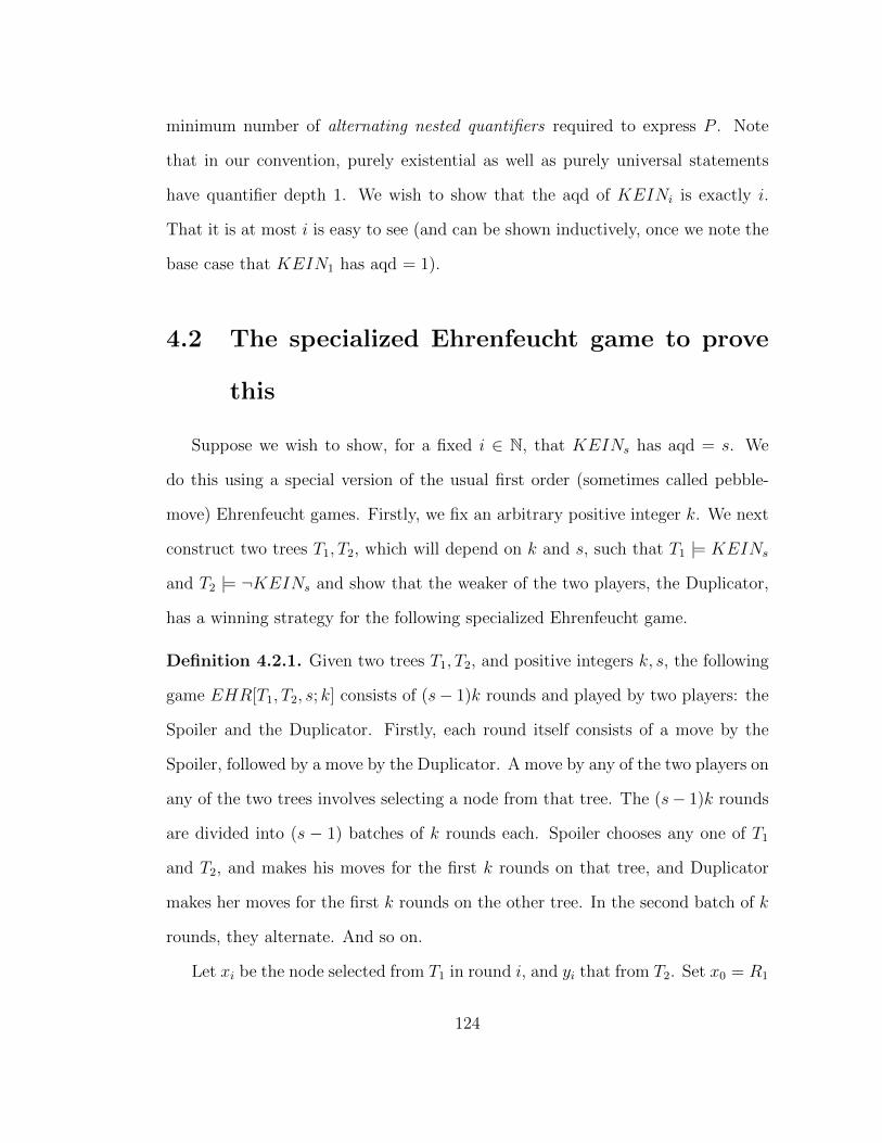
minimum number of alternating nested quantifiers required to express P . Note
that in our convention, purely existential as well as purely universal statements
have quantifier depth 1. We wish to show that the aqd of KEINi is exactly i.
That it is at most i is easy to see (and can be shown inductively, once we note the
base case that KEIN1 has aqd = 1).
4.2 The specialized Ehrenfeucht game to prove
this
Suppose we wish to show, for a fixed i ∈ N, that KEINs has aqd = s. We
do this using a special version of the usual first order (sometimes called pebble-
move) Ehrenfeucht games. Firstly, we fix an arbitrary positive integer k. We next
construct two trees T1, T2, which will depend on k and s, such that T1 |= KEINs
and T2 |= ¬KEINs and show that the weaker of the two players, the Duplicator,
has a winning strategy for the following specialized Ehrenfeucht game.
Definition 4.2.1. Given two trees T1, T2, and positive integers k, s, the following
game EHR[T1, T2, s; k] consists of (s− 1)k rounds and played by two players: the
Spoiler and the Duplicator. Firstly, each round itself consists of a move by the
Spoiler, followed by a move by the Duplicator. A move by any of the two players on
any of the two trees involves selecting a node from that tree. The (s− 1)k rounds
are divided into (s − 1) batches of k rounds each. Spoiler chooses any one of T1
and T2, and makes his moves for the first k rounds on that tree, and Duplicator
makes her moves for the first k rounds on the other tree. In the second batch of k
rounds, they alternate. And so on.
Let xi be the node selected from T1 in round i, and yi that from T2. Set x0 = R1
124
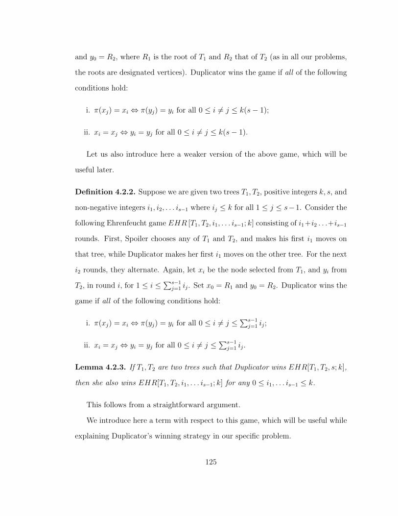
and y0 = R2, where R1 is the root of T1 and R2 that of T2 (as in all our problems,
the roots are designated vertices). Duplicator wins the game if all of the following
conditions hold:
i. π(xj) = xi ⇔ π(yj) = yi for all 0 ≤ i 6= j ≤ k(s− 1);
ii. xi = xj ⇔ yi = yj for all 0 ≤ i 6= j ≤ k(s− 1).
Let us also introduce here a weaker version of the above game, which will be
useful later.
Definition 4.2.2. Suppose we are given two trees T1, T2, positive integers k, s, and
non-negative integers i1, i2, . . . is−1 where ij ≤ k for all 1 ≤ j ≤ s−1. Consider the
following Ehrenfeucht game EHR [T1, T2, i1, . . . is−1; k] consisting of i1+i2 . . .+is−1
rounds. First, Spoiler chooses any of T1 and T2, and makes his first i1 moves on
that tree, while Duplicator makes her first i1 moves on the other tree. For the next
i2 rounds, they alternate. Again, let xi be the node selected from T1, and yi from
T2, in round i, for 1 ≤ i ≤∑s−1j=1 ij. Set x0 = R1 and y0 = R2. Duplicator wins the
game if all of the following conditions hold:
i. π(xj) = xi ⇔ π(yj) = yi for all 0 ≤ i 6= j ≤∑s−1j=1 ij;
ii. xi = xj ⇔ yi = yj for all 0 ≤ i 6= j ≤∑s−1j=1 ij.
Lemma 4.2.3. If T1, T2 are two trees such that Duplicator wins EHR[T1, T2, s; k],
then she also wins EHR[T1, T2, i1, . . . is−1; k] for any 0 ≤ i1, . . . is−1 ≤ k.
This follows from a straightforward argument.
We introduce here a term with respect to this game, which will be useful while
explaining Duplicator’s winning strategy in our specific problem.
125
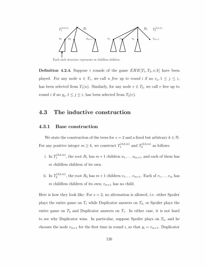
R1
u1 u2 um+1
R2
v1 v2 vk vm+1
Each such structure represents m childless children.
T(2,k,m)1 T
(2,k,m)2
Definition 4.2.4. Suppose i rounds of the game EHR [T1, T2, s; k] have been
played. For any node u ∈ T1, we call u free up to round i if no xj, 1 ≤ j ≤ i,
has been selected from T1(u). Similarly, for any node v ∈ T2, we call v free up to
round i if no yj, 1 ≤ j ≤ i, has been selected from T2(v).
4.3 The inductive construction
4.3.1 Base construction
We state the construction of the trees for s = 2 and a fixed but arbitrary k ∈ N.
For any positive integer m ≥ k, we construct T(2,k,m)1 and T
(2,k,m)2 as follows:
i. In T(2,k,m)1 , the root R1 has m+ 1 children u1, . . . um+1, and each of them has
m childless children of its own.
ii. In T(2,k,m)2 , the root R2 has m+ 1 children v1, . . . vm+1. Each of v1, . . . vm has
m childless children of its own; vm+1 has no child.
Here is how they look like: For s = 2, no alternation is allowed, i.e. either Spoiler
plays the entire game on T1 while Duplicator answers on T2, or Spoiler plays the
entire game on T2 and Duplicator answers on T1. In either case, it is not hard
to see why Duplicator wins. In particular, suppose Spoiler plays on T2, and he
chooses the node vm+1 for the first time in round i, so that yi = vm+1. Duplicator
126
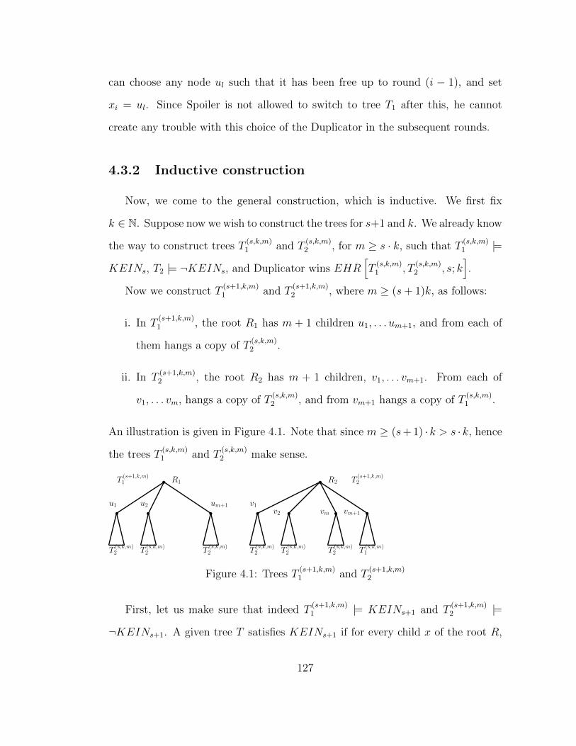
can choose any node ul such that it has been free up to round (i − 1), and set
xi = ul. Since Spoiler is not allowed to switch to tree T1 after this, he cannot
create any trouble with this choice of the Duplicator in the subsequent rounds.
4.3.2 Inductive construction
Now, we come to the general construction, which is inductive. We first fix
k ∈ N. Suppose now we wish to construct the trees for s+1 and k. We already know
the way to construct trees T(s,k,m)1 and T
(s,k,m)2 , for m ≥ s · k, such that T
(s,k,m)1 |=
KEINs, T2 |= ¬KEINs, and Duplicator wins EHR[T
(s,k,m)1 , T
(s,k,m)2 , s; k
].
Now we construct T(s+1,k,m)1 and T
(s+1,k,m)2 , where m ≥ (s+ 1)k, as follows:
i. In T(s+1,k,m)1 , the root R1 has m + 1 children u1, . . . um+1, and from each of
them hangs a copy of T(s,k,m)2 .
ii. In T(s+1,k,m)2 , the root R2 has m + 1 children, v1, . . . vm+1. From each of
v1, . . . vm, hangs a copy of T(s,k,m)2 , and from vm+1 hangs a copy of T
(s,k,m)1 .
An illustration is given in Figure 4.1. Note that since m ≥ (s+ 1) · k > s · k, hence
the trees T(s,k,m)1 and T
(s,k,m)2 make sense.
u1 u2 um+1 v1v2 vm vm+1
T(s,k,m)2 T
(s,k,m)2 T
(s,k,m)2 T
(s,k,m)2 T
(s,k,m)2 T
(s,k,m)2 T
(s,k,m)1
R1 R2T(s+1,k,m)1 T
(s+1,k,m)2
Figure 4.1: Trees T(s+1,k,m)1 and T
(s+1,k,m)2
First, let us make sure that indeed T(s+1,k,m)1 |= KEINs+1 and T
(s+1,k,m)2 |=
¬KEINs+1. A given tree T satisfies KEINs+1 if for every child x of the root R,
127
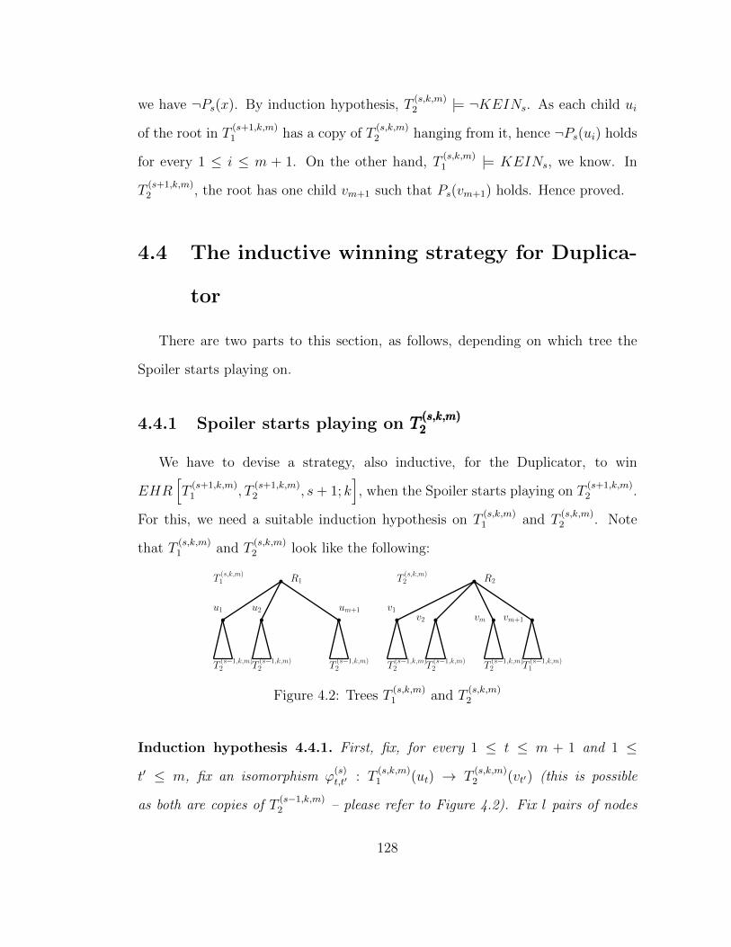
we have ¬Ps(x). By induction hypothesis, T(s,k,m)2 |= ¬KEINs. As each child ui
of the root in T(s+1,k,m)1 has a copy of T
(s,k,m)2 hanging from it, hence ¬Ps(ui) holds
for every 1 ≤ i ≤ m + 1. On the other hand, T(s,k,m)1 |= KEINs, we know. In
T(s+1,k,m)2 , the root has one child vm+1 such that Ps(vm+1) holds. Hence proved.
4.4 The inductive winning strategy for Duplica-
tor
There are two parts to this section, as follows, depending on which tree the
Spoiler starts playing on.
4.4.1 Spoiler starts playing on T(s,k,m)2T(s,k,m)2T(s,k,m)2
We have to devise a strategy, also inductive, for the Duplicator, to win
EHR[T
(s+1,k,m)1 , T
(s+1,k,m)2 , s+ 1; k
], when the Spoiler starts playing on T
(s+1,k,m)2 .
For this, we need a suitable induction hypothesis on T(s,k,m)1 and T
(s,k,m)2 . Note
that T(s,k,m)1 and T
(s,k,m)2 look like the following:
R1 R2
u1 u2 um+1 v1v2 vm vm+1
T(s−1,k,m)2 T
(s−1,k,m)2 T
(s−1,k,m)2 T
(s−1,k,m)2 T
(s−1,k,m)2 T
(s−1,k,m)2 T
(s−1,k,m)1
T(s,k,m)1 T
(s,k,m)2
Figure 4.2: Trees T(s,k,m)1 and T
(s,k,m)2
Induction hypothesis 4.4.1. First, fix, for every 1 ≤ t ≤ m + 1 and 1 ≤
t′ ≤ m, fix an isomorphism ϕ(s)t,t′ : T
(s,k,m)1 (ut) → T
(s,k,m)2 (vt′) (this is possible
as both are copies of T(s−1,k,m)2 – please refer to Figure 4.2). Fix l pairs of nodes
128
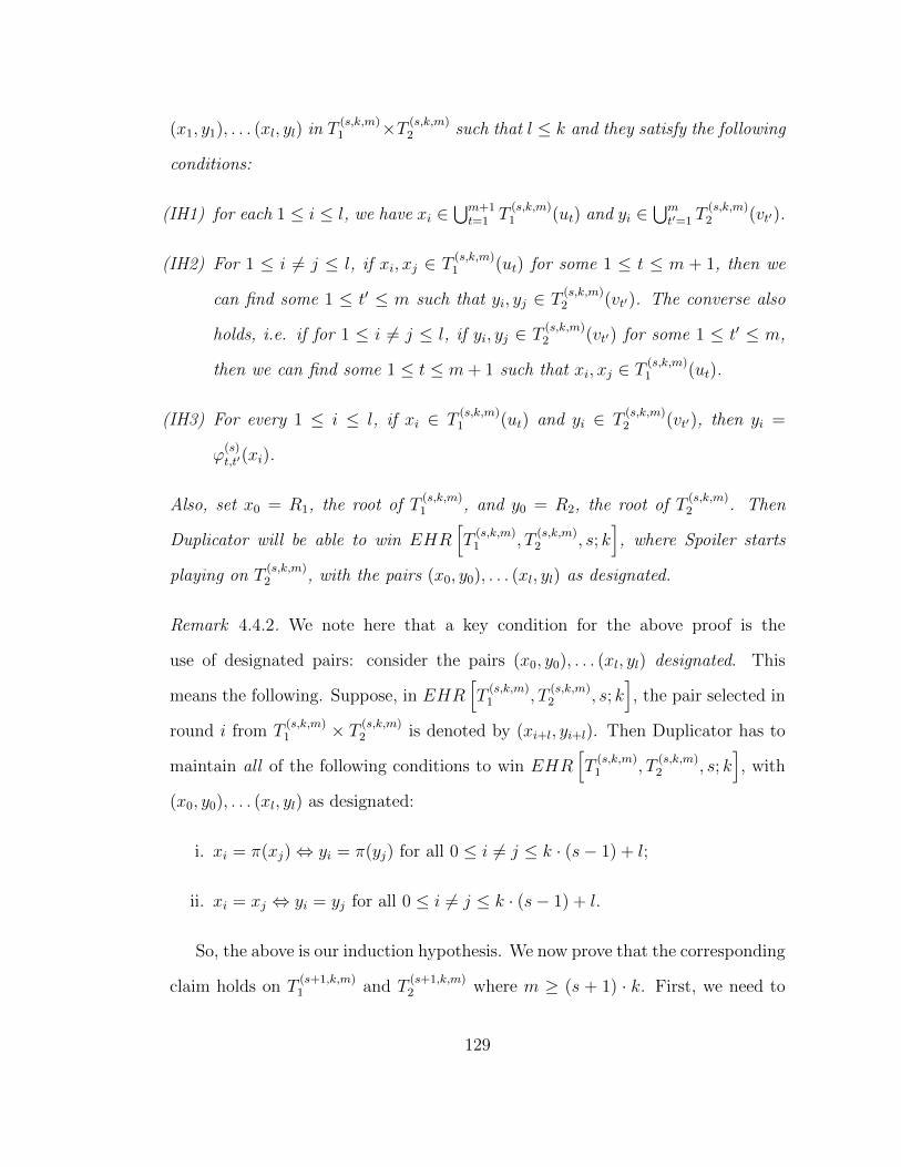
(x1, y1), . . . (xl, yl) in T(s,k,m)1 ×T (s,k,m)
2 such that l ≤ k and they satisfy the following
conditions:
(IH1) for each 1 ≤ i ≤ l, we have xi ∈⋃m+1t=1 T
(s,k,m)1 (ut) and yi ∈
⋃mt′=1 T
(s,k,m)2 (vt′).
(IH2) For 1 ≤ i 6= j ≤ l, if xi, xj ∈ T (s,k,m)1 (ut) for some 1 ≤ t ≤ m + 1, then we
can find some 1 ≤ t′ ≤ m such that yi, yj ∈ T (s,k,m)2 (vt′). The converse also
holds, i.e. if for 1 ≤ i 6= j ≤ l, if yi, yj ∈ T (s,k,m)2 (vt′) for some 1 ≤ t′ ≤ m,
then we can find some 1 ≤ t ≤ m+ 1 such that xi, xj ∈ T (s,k,m)1 (ut).
(IH3) For every 1 ≤ i ≤ l, if xi ∈ T(s,k,m)1 (ut) and yi ∈ T
(s,k,m)2 (vt′), then yi =
ϕ(s)t,t′(xi).
Also, set x0 = R1, the root of T(s,k,m)1 , and y0 = R2, the root of T
(s,k,m)2 . Then
Duplicator will be able to win EHR[T
(s,k,m)1 , T
(s,k,m)2 , s; k
], where Spoiler starts
playing on T(s,k,m)2 , with the pairs (x0, y0), . . . (xl, yl) as designated.
Remark 4.4.2. We note here that a key condition for the above proof is the
use of designated pairs: consider the pairs (x0, y0), . . . (xl, yl) designated. This
means the following. Suppose, in EHR[T
(s,k,m)1 , T
(s,k,m)2 , s; k
], the pair selected in
round i from T(s,k,m)1 × T (s,k,m)
2 is denoted by (xi+l, yi+l). Then Duplicator has to
maintain all of the following conditions to win EHR[T
(s,k,m)1 , T
(s,k,m)2 , s; k
], with
(x0, y0), . . . (xl, yl) as designated:
i. xi = π(xj)⇔ yi = π(yj) for all 0 ≤ i 6= j ≤ k · (s− 1) + l;
ii. xi = xj ⇔ yi = yj for all 0 ≤ i 6= j ≤ k · (s− 1) + l.
So, the above is our induction hypothesis. We now prove that the corresponding
claim holds on T(s+1,k,m)1 and T
(s+1,k,m)2 where m ≥ (s + 1) · k. First, we need to
129
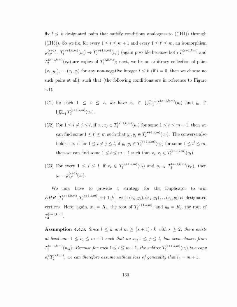
fix l ≤ k designated pairs that satisfy conditions analogous to ((IH1)) through
((IH3)). So we fix, for every 1 ≤ t ≤ m+ 1 and every 1 ≤ t′ ≤ m, an isomorphism
ϕ(s+1)t,t′ : T
(s+1,k,m)1 (ut)→ T
(s+1,k,m)2 (vt′) (again possible because both T
(s+1,k,m)1 and
T(s+1,k,m)2 (vt′) are copies of T
(s,k,m)2 ); next, we fix an arbitrary collection of pairs
(x1, y1), . . . (xl, yl) for any non-negative integer l ≤ k (if l = 0, then we choose no
such pairs at all), such that (the following conditions are in reference to Figure
4.1):
(C1) for each 1 ≤ i ≤ l, we have xi ∈⋃m+1t=1 T
(s+1,k,m)1 (ut) and yi ∈⋃m
t′=1 T(s+1,k,m)2 (vt′).
(C2) For 1 ≤ i 6= j ≤ l, if xi, xj ∈ T (s+1,k,m)1 (ut) for some 1 ≤ t ≤ m + 1, then we
can find some 1 ≤ t′ ≤ m such that yi, yj ∈ T (s+1,k,m)2 (vt′). The converse also
holds, i.e. if for 1 ≤ i 6= j ≤ l, if yi, yj ∈ T (s+1,k,m)2 (vt′) for some 1 ≤ t′ ≤ m,
then we can find some 1 ≤ t ≤ m+ 1 such that xi, xj ∈ T (s+1,k,m)1 (ut).
(C3) For every 1 ≤ i ≤ l, if xi ∈ T(s+1,k,m)1 (ut) and yi ∈ T
(s+1,k,m)2 (vt′), then
yi = ϕ(s+1)t,t′ (xi).
We now have to provide a strategy for the Duplicator to win
EHR[T
(s+1,k,m)1 , T
(s+1,k,m)2 , s+ 1; k
], with (x0, y0), (x1, y1) . . . (xl, yl) as designated
vertices. Here, again, x0 = R1, the root of T(s+1,k,m)1 , and y0 = R2, the root of
T(s+1,k,m)2 .
Assumption 4.4.3. Since l ≤ k and m ≥ (s + 1) · k with s ≥ 2, there exists
at least one 1 ≤ i0 ≤ m + 1 such that no xj, 1 ≤ j ≤ l, has been chosen from
T(s+1,k,m)1 (ui0). Because for each 1 ≤ i ≤ m+ 1, the subtree T
(s+1,k,m)1 (ui) is a copy
of T(s,k,m)2 , we can therefore assume without loss of generality that i0 = m+ 1.
130
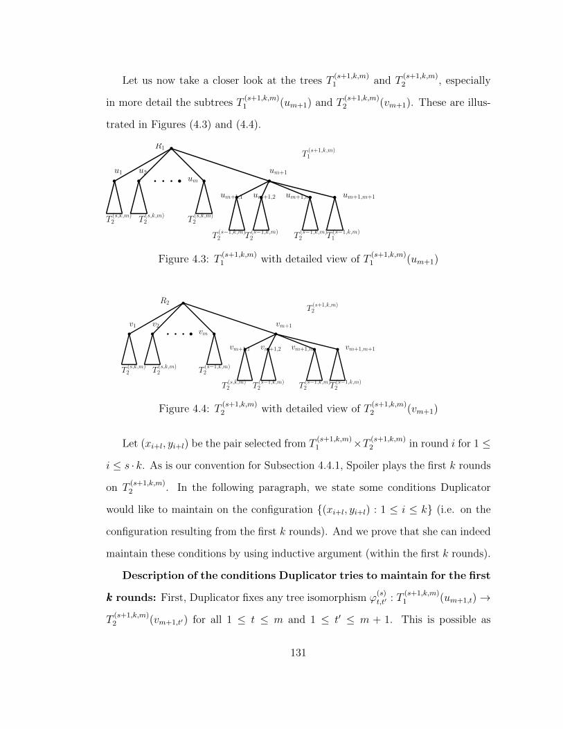
Let us now take a closer look at the trees T(s+1,k,m)1 and T
(s+1,k,m)2 , especially
in more detail the subtrees T(s+1,k,m)1 (um+1) and T
(s+1,k,m)2 (vm+1). These are illus-
trated in Figures (4.3) and (4.4).
R1
u1 u2um
T(s,k,m)2 T
(s,k,m)2 T
(s,k,m)2
um+1
um+1,1 um+1,2 um+1,m um+1,m+1
T(s−1,k,m)2 T
(s−1,k,m)2 T
(s−1,k,m)2 T
(s−1,k,m)1
T(s+1,k,m)1
Figure 4.3: T(s+1,k,m)1 with detailed view of T
(s+1,k,m)1 (um+1)
v1 v2vm
T(s,k,m)2 T
(s,k,m)2 T
(s−1,k,m)2
vm+1
vm+1,1 vm+1,2 vm+1,m vm+1,m+1
T(s,k,m)2 T
(s−1,k,m)2 T
(s−1,k,m)2 T
(s−1,k,m)2
T(s+1,k,m)2
R2
Figure 4.4: T(s+1,k,m)2 with detailed view of T
(s+1,k,m)2 (vm+1)
Let (xi+l, yi+l) be the pair selected from T(s+1,k,m)1 ×T (s+1,k,m)
2 in round i for 1 ≤
i ≤ s · k. As is our convention for Subsection 4.4.1, Spoiler plays the first k rounds
on T(s+1,k,m)2 . In the following paragraph, we state some conditions Duplicator
would like to maintain on the configuration (xi+l, yi+l) : 1 ≤ i ≤ k (i.e. on the
configuration resulting from the first k rounds). And we prove that she can indeed
maintain these conditions by using inductive argument (within the first k rounds).
Description of the conditions Duplicator tries to maintain for the first
kkk rounds: First, Duplicator fixes any tree isomorphism ϕ(s)t,t′ : T
(s+1,k,m)1 (um+1,t)→
T(s+1,k,m)2 (vm+1,t′) for all 1 ≤ t ≤ m and 1 ≤ t′ ≤ m + 1. This is possible as
131
each T(s+1,k,m)1 (um+1,t), 1 ≤ t ≤ m, as well as each T
(s+1,k,m)2 (vm+1,t′), 1 ≤ t′ ≤
m + 1, is a copy of T(s−1,k,m)2 . Suppose p ≤ k rounds of the game have been
played. The conditions on the configuration (xl+1, yl+1), . . . (xl+p, yl+p) are as
follows (Assumption 4.4.3 is made throughout):
(A1) xi+l = R1 ⇔ yi+l = R2. If xi+l ∈ T (s+1,k,m)1 (ut) for some 1 ≤ t ≤ m, then
yi+l ∈ T (s+1,k,m)2 (vt′) for some 1 ≤ t′ ≤ m, and vice versa; moreoever, in this
case, yi+l = ϕs+1t,t′ (xi+l).
If xi+l ∈ T(s+1,k,m)1 (um+1), then actually xi+l ∈ ⋃m
t=1 ∈
T(s+1,k,m)1 (um+1,t)
⋃um+1. If xi+l = um+1 then yi+l = vm+1, and
vice versa. If xi+l ∈ T(s+1,k,m)1 (um+1,t) for some 1 ≤ t ≤ m, then
yi+l ∈ T (s+1,k,m)2 (um+1,t′) for some 1 ≤ t′ ≤ m + 1, and vice versa; moreover,
in this case, yi+l = ϕ(s)t,t′(xi+l).
(A2) Suppose we have xi+l, xj ∈ T (s+1,k,m)1 (ut) for some 1 ≤ i ≤ p, 1 ≤ j ≤ p + l
such that j 6= i+ l, and some 1 ≤ t ≤ m. Then there exists some 1 ≤ t′ ≤ m
such that yi+l, yj ∈ T (s+1,k,m)2 (vt′).
The converse of this statement is true as well. That means, if for some
1 ≤ i ≤ p, 1 ≤ j ≤ p + l with j 6= i + l, and 1 ≤ t′ ≤ m, we have
yi+l, yj ∈ T(s+1,k,m)2 (vt′), then there exists some 1 ≤ t′ ≤ m such that
xi+l, xj ∈ T (s+1,k,m)1 (ut).
(A3) Suppose for 1 ≤ i 6= j ≤ p we have xi+l, xj+l ∈ T (s+1,k,m)1 (um+1,t) for some
1 ≤ t ≤ m. Then there exists 1 ≤ t′ ≤ m + 1 such that yi+l, yj+l ∈
T(s+1,k,m)2 (vm+1,t′). The converse of this statement is also true, i.e. if for
1 ≤ i 6= j ≤ p, we have yi+l, yj+l ∈ T (s+1,k,m)2 (vm+1,t′) for some 1 ≤ t′ ≤ m+1,
then there exists 1 ≤ t ≤ m such that xi+l, xj+l ∈ T (s+1,k,m)1 (um+1,t).
132
How does the Duplicator maintain all these conditions for the first k rounds?
We show this by induction on p, where p < k is the number of rounds played so
far. Suppose Duplicator has been able to maintain all these conditions up to (and
including) round p where p < k. Now, Spoiler chooses yl+p+1 from T(s+1,k,m)2 . Here
is how Duplicator replies:
i. If yp+l+1 = R2, the root of T(s+1,k,m)2 , then Duplicator chooses xp+l+1 = R1,
the root of T(s+1,k,m)1 .
ii. Suppose yp+l+1 ∈⋃mt′=1 T
(s+1,k,m)2 (vt′). Then there are a few possible cases,
as follows:
(a) Suppose there exists 1 ≤ j ≤ l+p such that yj and yp+l+1 both belong to
the same T(s+1,k,m)2 (vt′) for some 1 ≤ t′ ≤ m. Then Duplicator finds the
t such that xj ∈ T (s+1,k,m)1 (ut). Note that if 1 ≤ j ≤ l, then 1 ≤ t ≤ m
because of Assumption 4.4.3), and if l + 1 ≤ j ≤ p+ l, then 1 ≤ t ≤ m
because of induction hypothesis Condition (A1). Then Duplicator sets
xp+l+1 =ϕ
(s+1)t,t′
−1
(yp+l+1).
(b) Suppose yp+l+1 ∈ T(s+1,k,m)2 (vt′) for some 1 ≤ t′ ≤ m, such that yj /∈
T(s+1,k,m)2 (vt′) for all 1 ≤ j ≤ l + p. Then Duplicator finds a 1 ≤ t ≤ m
such that ut is free up to round p (recall Definition 4.2.4). She can
always find such a t as m ≥ (s + 1) · k > 2k > p + l. She then sets
xp+l+1 =ϕ
(s+1)t,t′
−1
(yp+l+1).
iii. Now suppose yp+l+1 ∈ T (s+1,k,m)2 (vm+1). Again, there are a few possible cases:
(a) If yp+l+1 = vm+1, then Duplicator sets xp+l+1 = um+1.
133
(b) If yp+l+1 ∈ T (s+1,k,m)2 (vm+1,t′) for some 1 ≤ t′ ≤ m + 1 such that there
exists some 1 ≤ i ≤ p with yi+l ∈ T(s+1,k,m)2 (vm+1,t′), then Duplicator
finds the t (where 1 ≤ t ≤ m by induction hypothesis (A1)) such that
xi+l ∈ T (s+1,k,m)1 (um+1,t). Then she sets xp+l+1 =
ϕ
(s)t,t′
−1
(yp+l+1).
(c) If yp+l+1 ∈ T (s+1,k,m)2 (vm+1,t′) for some 1 ≤ t′ ≤ m + 1 such that yi+l /∈
T(s+1,k,m)2 (vm+1,t′) for all 1 ≤ i ≤ p, then Duplicator finds a 1 ≤ t ≤ m
such that um+1,t is free up to round p (again, possible since m ≥ (s +
1) · k > k ≥ p+ 1) and sets xp+l+1 =ϕ
(s)t,t′
−1
(yp+l+1).
Focus now on T(s+1,k,m)2 (vm+1)T(s+1,k,m)2 (vm+1)T(s+1,k,m)2 (vm+1) and T
(s+1,k,m)1 (um+1)T(s+1,k,m)1 (um+1)T(s+1,k,m)1 (um+1) only: Suppose the
only pairs selected up to round k that are in T(s+1,k,m)1 (um+1) × T (s+1,k,m)
2 (vm+1)
are (xi1+l, yi1+l) , . . . (xir+l, yir+l). Now, T(s+1,k,m)1 (um+1) is a copy of T
(s,k,m)2 and
T(s+1,k,m)2 (vm+1) is a copy of T
(s,k,m)1 . From (A1) and (A3), we can see that the
pairs (yi1+l, xi1+l), . . . (yir+l, xir+l) satisfy Conditions (IH1) through (IH3).
Conclusion 4.4.4. So Duplicator, by induction hypothesis, will
win EHR[T(s+1,k,m)2 (vm+1), T
(s+1,k,m)1 (um+1), s; k] with designated pairs
(yi1+l, xi1+l), . . . (yir+l, xir+l) (notice the deliberate writing of T(s+1,k,m)2 (vm+1)
before T(s+1,k,m)1 (um+1)).
Now consider the subsequent game of remaining (s−1) ·k rounds. We call this
the second part of the game. For this part of the game, we really can split the tree
T(s+1,k,m)1 into
R1 ∪ S1 ∪ T (s+1,k,m)1 (um+1), where S1 =
m⋃t=1
T(s+1,k,m)1 (ut)
, (4.1)
134
and the tree T(s+1,k,m)2 into
R2 ∪ S2 ∪ T (s+1,k,m)2 (vm+1), where S2 =
m⋃t′=1
T(s+1,k,m)1 (vt′)
. (4.2)
Suppose p rounds of the game have been played, with k < p ≤ sk. Duplicator
maintains the following conditions on the configuration (xi, yi) : 0 ≤ i ≤ p+ l:
(B1) xi = R1 ⇔ yi = R2.
(B2) xi ∈ S1 ⇔ yi = S2. In this case, if xi ∈ T (s+1,k,m)1 (ut) for some 1 ≤ t ≤ m
and yi ∈ T (s+1,k,m)2 (vt′), then yi = ϕ
(s+1)t,t′ (xi).
(B3) If xi, xi′ ∈ T (s+1,k,m)1 (ut) for some 1 ≤ t ≤ m, then there exists 1 ≤ t′ ≤ m
with yi, yi′ ∈ T (s+1,k,m)2 (vt′).
(B4) xi ∈ T (s+1,k,m)1 (um+1)⇔ yi ∈ T (s+1,k,m)
2 (vm+1). Suppose (i−1)k+1 ≤ p ≤ ik,
where 2 ≤ i ≤ s. Suppose the number of pairs of nodes selected from
T(s+1,k,m)2 (vm+1) × T
(s+1,k,m)1 (um+1) between rounds k + 1 and 2k is j1;
between rounds 2k + 1 and 3k is j2; . . . between rounds (i − 2)k + 1 and
(i−1)k is ji−2; between rounds (i−1)k+1 and p is j′. Then Duplicator wins
EHR[T
(s+1,k,m)2 (vm+1), T
(s+1,k,m)1 (um+1), j1, j2, . . . ji−2, j
′ + ik − p, k, . . . , k; k]
with designated pairs (yi1+l, xi1+l), . . . (yir+l, xir+l), where the first
j1 + j2 + . . . ji−2 + j′ rounds have been played out, with Spoiler start-
ing on T(s+1,k,m)1 (um+1).
It is not hard to see that the Duplicator is able to maintain all the conditions
stated above. She is able to maintain the last condition because of Conclusion
4.4.4 and Lemma 4.2.3. This brings us to the end of the inductive proof.
135
4.4.2 When Spoiler starts playing on T(s,k,m)1T(s,k,m)1T(s,k,m)1
The construction remains the same as before. The induction hypothesis in this
case is simpler to state.
Induction hypothesis 4.4.5. Duplicator wins EHR[T
(s,k,m)1 , T
(s,k,m)2 , s; k
]when
Spoiler starts on T(s,k,m)1 .
Let us do the proof by induction. Refer to Figures 4.3 and 4.4. Again, we
chalk out the detailed strategy of the Duplicator for the first k rounds, where we
do not use Induction hypothesis 4.4.5. For every 1 ≤ t ≤ m + 1 and 1 ≤ t′ ≤ m,
she fixes any tree isomorphism ϕ(s+1)t,t′ : T
(s+1,k,m)1 (ut) → T
(s+1,k,m)2 (vt′). This is
possible since each of T(s+1,k,m)1 (ut) and T
(s+1,k,m)2 (vt′) is a copy of T
(s,k,m)2 for all
1 ≤ t ≤ m+ 1, 1 ≤ t′ ≤ m. For the first p rounds, for all 1 ≤ p ≤ k, she maintains
the following conditions on the configuration (xi, yi) : 1 ≤ i ≤ p:
(A’1) xi = R1 ⇔ yi = R2.
(A’2) If xi ∈ T(s+1,k,m)1 (ut) for some 1 ≤ t ≤ m + 1, then yi ∈ T
(s+1,k,m)2 (vt′) for
some 1 ≤ t′ ≤ m. Furthermore yi = ϕ(s+1)t,t′ (xi).
(A’3) If xi, xj ∈ T(s+1,k,m)1 (ut) for some 1 ≤ i 6= j ≤ p, then there exists some
1 ≤ t′ ≤ m such that yi, yj ∈ T (s+1,k,m)2 (vt′).
That the Duplicator is able to maintain these conditions can be shown by
induction on p where 1 ≤ p ≤ k − 1. So, suppose the first p rounds have been
played. In the (p + 1)-st round Spoiler chooses xp+1 from T(s+1,k,m)1 . Duplicator
replies as follows:
i. If xp+1 = R1, then Duplicator sets yp+1 = R2.
136
ii. If xp+1 ∈ T(s+1,k,m)1 (ut) for some 1 ≤ t ≤ m + 1 such that there exists
some 1 ≤ j ≤ p with xj ∈ T (s+1,k,m)1 (ut) as well, then Duplicator finds the
1 ≤ t′ ≤ m such that yj ∈ T (s+1,k,m)2 (vt′) and sets yp+1 = ϕ
(s+1)t,t′ (xp+1).
iii. If xp+1 ∈ T (s+1,k,m)1 (ut) for some 1 ≤ t ≤ m + 1 such that xj /∈ T (s+1,k,m)
1 (ut)
for all 1 ≤ j ≤ p, then Duplicator finds 1 ≤ t′ ≤ m such that vt′ has been free
up to round p. She can always find such a vt′ since m ≥ (s + 1)k > 2k > p.
Then she sets yp+1 = ϕ(s+1)t,t′ (xp+1).
Assumption 4.4.6. Since m ≥ (s+ 1)k > 2k > k, hence there will be at least one
1 ≤ i0 ≤ m + 1 such that ui0 is free up to round k. Since for all 1 ≤ t ≤ m + 1,
T(s+1,k,m)1 (ut) is a copy of T
(s,k,m)2 , hence we can assume without loss of generality
that i0 = m+ 1.
Now, once again, we come to the second part of the game, where there are
(s − 1)k rounds, and the Spoiler plays the first set of k rounds of this part on
T(s+1,k,m)2 . We make Assumption 4.4.6 throughout. Note that T
(s+1,k,m)1 (um+1) is
a copy of T(s,k,m)2 whereas T
(s+1,k,m)2 (vm+1) is a copy of T
(s,k,m)1 .
Conclusion 4.4.7. By induction hypothesis, Duplicator wins
EHR[T
(s+1,k,m)2 (vm+1), T
(s+1,k,m)1 (um+1), s; k
]when Spoiler starts playing on
T(s+1,k,m)2 (vm+1).
We can again split up the two trees as follows:
T(s+1,k,m)1 = R1 ∪ S1 ∪ T (s+1,k,m)
1 (um+1), where S1 =m⋃t=1
T(s+1,k,m)1 (ut), (4.3)
137
and
T(s+1,k,m)2 = R2 ∪ S2 ∪ T (s+1,k,m)
2 (vm+1), where S2 =m⋃t′=1
T(s+1,k,m)2 (vt′). (4.4)
In the second part of the game, for every k ≤ p ≤ sk, Duplicator maintains the
following conditions on the configuration (xi, yi) : 1 ≤ i ≤ p:
i. xi = R1 ⇔ yi = R2.
ii. xi ∈ S1 ⇔ yi ∈ S2. If xi ∈ T(s+1,k,m)1 (ut) for some 1 ≤ t ≤ m and yi ∈
T(s+1,k,m)2 (vt′) for some 1 ≤ t′ ≤ m, then yi = ϕ
(s+1)t,t′ (xi).
iii. If for 1 ≤ i 6= j ≤ p, we have xi, xj ∈ T (s+1,k,m)1 (ut) for some 1 ≤ t ≤ m, then
there exists some 1 ≤ t′ ≤ m with yi, yj ∈ T (s+1,k,m)2 (vt′).
iv. xi ∈ T (s+1,k,m)1 (um+1)⇔ yi ∈ T (s+1,k,m)
2 (vm+1). Suppose (i−1)k+1 ≤ p ≤ ik,
where 2 ≤ i ≤ s. Suppose the number of pairs of nodes selected from
T(s+1,k,m)2 (vm+1) × T
(s+1,k,m)1 (um+1) between rounds k + 1 and 2k is j1;
between rounds 2k + 1 and 3k is j2; . . . between rounds (i − 2)k + 1 and
(i−1)k is ji−2; between rounds (i−1)k+1 and p is j′. Then Duplicator wins
EHR[T
(s+1,k,m)2 (vm+1), T
(s+1,k,m)1 (um+1), j1, j2, . . . ji−2, j
′ + ik − p, k, . . . , k; k],
where the first j1 + j2 + . . . ji−2 + j′ rounds have been played out, with
Spoiler starting on T(s+1,k,m)2 (um+1).
Again, it is not hard to see that the Duplicator is able to maintain all the
conditions stated above. She is able to maintain the last condition because of
Conclusion 4.4.7 and Lemma 4.2.3. This brings us to the end of the inductive
proof.
138
Bibliography
[1] J. Spencer and L. Thoma, On the limit values of probabilities for the first order
properties of graphs, Contemporary trends in discrete mathematics (Stirın
Castle, 1997), DIMACS Ser. Discrete Math. Theoret. Comput. Sci. Amer.
Math. Soc. Providence, RI, 1999; Vol. 49; Pages: 317–336.
[2] J. Spencer and N. Alon, The Probabilistic Method, Wiley-Interscience Series
in Discrete Mathematics and Optimization, John Wiley & Sons, Inc., Hobo-
ken, NJ, 2008; ISBN:978-0-470-17020-5.
[3] R. van der Hofstad, Random Graphs and Complex Networks, Vol 1, Lecture
Notes, http://www.win.tue.nl/~rhofstad/NotesRGCN.pdf, 2015.
[4] M. Podder and J. Spencer, First Order Probabilities For Galton-Watson Trees,
to appear in A Journey Through Discrete Mathematics: A Tribute to Jiri
Matousek, Springer International Publishing Switzerland, 2017, ISBN:978-3-
319-44478-9.
[5] J. Spencer, The Strange Logic of Random Graphs, Springer Publishing
Company, Inc. 2010; Series : Algorithms and Combinatorics, Vol. 22;
ISBN:3642074995 9783642074998.
139
[6] D. A. Levin, Y. Peres and E. L. Wilmer, Markov Chains and Mixing Times,
American Mathematical Society, 2006; ISBN: 978-0-8218-4739-8.
[7] N. Immerman, Descriptive complexity, Springer Science & Business Media,
2012; ISBN-13: 978-0387986005.
[8] D. Marker, Model theory: an introduction, Springer Science & Business Me-
dia, 2006; ISBN: 978-1-4419-3157-3.
[9] H. Kesten, Subdiffusive behavior of random walk on a random cluster, Ann.
Inst. H. Poincare Probab. Statist., Volume 22, Number 4, Pages 425–487,
1986.
[10] K. B. Athreya, and P. E. Ney, Branching processes, Springer Science & Busi-
ness Media, Volume 196, 2012.
[11] R. Lyons and Y. Peres, Probability on Trees and Networks, Cambridge Uni-
versity Press, New York, xvi+699, 2016, available at http://pages.iu.edu/
~rdlyons/.
[12] H. Comon, M. Dauchet, R. Gilleron, C. Loding, F. Jacquemard, D. Lugiez,
S. Tison and M. Tommasi, Tree automata techniques and applications, 2007,
file:///home/podder/Downloads/tata.pdf.
[13] T. E. Harris, The theory of branching processes, Courier Corporation, 2002.
[14] S. Janson, Svante, Simply generated trees, conditioned Galton-Watson trees,
random allocations and condensation, Probab. Surv, Volume 9, Pages 103–
252, 2012.
140