the strategies of new technology adoption under real
TRANSCRIPT

1
The Strategies of New Technology Adoption under Real Options:
Laboratory Experiment
Besma Teffahi1 and Walid Hichri2
Abstract
In this paper we test, by organizing experimental economics sessions, the main results of real-
option theory on the strategies of new technology adoption. Thus, we verify, in a first game,
the results of Grenadier and Weiss (GW) (1997) concerning the different strategies that the firm
can undertake. In a second game of duopoly, we consider the models of Smit and Trigeorgis
(2004, Chapter 5) and Huissman and Kort (HK) (2004). We evaluate risk aversion (RA)
through Holt and Laury's (2002) lottery and the cognitive reflection test (CRT) through
Frederick (2005). Then, we investigate whether risk aversion and /or cognitive ability reinforces
cooperation and thus waiting behavior.
Keywords: technology adoption, real options, game theory, experimental economics
I - Theoretical model and concept of experience
Under the RO approach, optimal investment behavior changes if the decision maker considers
that the decision to invest may be delayed for at least one period. The postponement of the
investment decision is useful as new information on the expected current value may be available
in the following period. It is considered that a rational decision-maker would invest immediately
only if the expected NPV is greater than the expected NPV a period later.
I-1-Theoretical model and hypothesis formulation
This model is closely related to Dixit and Pindyck (1994). Suppose agents maximize their
profits and are offered a contract to exercise it now or wait until period 1 when all uncertainties
about the results are revealed before making the investment decision.
The way we operate the flows of projects today affects not only the profits of today, but also
those of tomorrow, because the stock that remains at the end of period 0 is only the one on
[email protected]. Phone :0021655135474. Address :Manouba University, High
Business School, Tunis, Tunisia 2 [email protected]

2
which we leave in period 1. In fact, optimal management cannot be achieved period by period,
as if these periods were independent of each other. Since current decisions have an impact on
future outcomes, the entire sequence of optimal decisions, at all times, must be resolved at once.
It is the mathematical tool that provides us with the appropriate method to accomplish this feat:
it is the dynamic programming founded by Bellman.
We are considering an ANT project with a limited lifespan and currently generating annual cash
flow. This flow follows an MBG.
𝑑𝑋𝑡 = 𝛼𝑋𝑡𝑑𝑡 + 𝜎𝑋𝑡𝑍𝑡
𝛼 and represents drift and volatility respectively and 𝜎𝑑𝑍𝑡~𝑁(0, 𝑑𝑡).
The risk-neutral version of a DP MBG (1994) is:3
𝑑𝑋𝑡 = (𝛼−𝜆)𝑋𝑡𝑑𝑡 + 𝜎𝑋𝑡𝑍𝑡
We can therefore deduce that:
𝐸(𝑋𝑡) = 𝑋0𝑒(𝛼−𝜆)𝑡 (1)
𝑉(𝑋𝑡) = 𝑋02𝑒2(𝛼−𝜆)𝑡(𝑒𝜎2𝑡 − 1) ≈ 𝑋0
2𝜎2∆𝑡 (2)
In this case of MBG, it is possible to deduct closed solutions for the value of the option. This
case can be considered the borderline case where the decision period is so long that it can
reasonably be addressed by the assumption of unlimited maturity. In other words, the expiration
time of the option tends to infinity. However, technological obsolescence or technological
progress limits project life, the analysis had to be modified to take into account the case where
the lifespan is over. Or T this lifespan, for which production ensures cash flows over T years.
In continuous time, cash flows grow at a (𝜶 − 𝝀)rate, this amount received at the moment t
must be discounted at the rate r: So the current value of the annuity between two dates and
is:𝜏1𝜏2
𝑉𝐴(𝑋𝑡) = ∫ 𝐸(𝑋𝑡)𝜏2
𝜏1𝑒−𝑟𝑡𝑑𝑡 =
[𝑒(𝛼−𝜆−𝑟)𝜏2−𝑒(𝛼−𝜆−𝑟)𝜏1]
(𝛼−𝜆−𝑟)𝑋0 = 𝑥𝑋0 (3)
U.S. options, which can be exercised at any time until expiry, are an example of cash flows that
depend on future information. A rational decision in such circumstances must consider not only
past information, but also expectations regarding future events. This required drawing up a
3 Remember that in a risk-neutral context, all individuals are supposed to be risk-neutral. As such, they are only concerned with average or
expected values and not with the dispersion around these values.

3
diagram that would sum up all the possibilities that might arise as the future presented itself,
and then make the best decision in each case. To do this, several methods exist, including
binomial networks. Their basic premise is that uncertainty can at any time be represented by
two alternative states. A binary distribution (or Bernoulli distribution) is a discrete distribution
that can take up two values, with probabilities (p) and (1-p). This is the binomial approximation
CCR that we use to check the inputs of MBG. The CCR model is another simpler writing of the
B&S model.
To do this, suppose that the value of cash flows (𝑋), over a unit of time ∆𝑡, can:
• either increase (up) to reach 𝑋+ = 𝑢𝑋0 with a probability (𝑝)where 𝑢 > 1
• either decrease (down) to reach 𝑋− = 𝑑𝑋0 with a probability (1 − 𝑝), where 𝑑 < 1
The expectation and variance in this discrete case are then:
𝐸(𝑋) = ∑ 𝑥𝑖𝑛𝑖=1 𝑝𝑖 = 𝑝 𝑢𝑋0 + (1 − 𝑝)𝑑𝑋0 (4)
𝑉(𝑋) = 𝐸(𝑋2) − (𝐸(𝑋))2 = (𝑝𝑢2𝑋02 + (1 − 𝑝)𝑑2𝑋0
2) − (𝑝 𝑢𝑋0 + (1 − 𝑝)𝑑𝑋0)2 (5)
The CCR model aims to match as closely as possible to the probability distribution in the case
of the ongoing MBG process. To do this, it is enough to equalize the two expectations (2) and
(4) and the two variances (3) and (5) (respectively of the two continuous and discrete cases).
This equality should allow us to deduce the unknown parameters of the CCR model which are:
𝑝, 𝑢 𝑎𝑛𝑑 𝑑
However, since we only have two equations, there is no one-stop solution. We can initially
force one variable to take a certain value and then solve the other two. A practical choice of the
third condition is the hypothesis of the symmetry of the binomial tree: , this condition has the
property that an "up" 4𝑢 =1
𝑑 followed by a "down" , or vice versa, leaves the fixed value:
.𝑢𝑑𝑋0 = 𝑑𝑢𝑋0 = 𝑋0
We get three equations with three strangers. Using a certain approximation, we deduce the
following solutions:5
𝑝 =𝑒(𝛼−𝜆)∆𝑡 − 𝑑
𝑢 − 𝑑; 𝑢 = 𝑒𝜎√∆𝑡; 𝑑 = 𝑒−𝜎√∆𝑡
4 Indeed, the trellis or binomial tree recombines: an increase followed by a decrease leads to the same asset price as a decrease followed by an
increase (otherwise the number of knots would be significantly higher)
5 A good simple but profound explanation on the website of the University of Taiwan:https://www.ntu.edu.tw/

4
Options are valued at the end of the network (at the T expiration date), as their earnings at that
time are known. From these terminal gains, backward induction allows the current value of the
option to be calculated.
Below is an investment situation that deduces the NPV approach and the OR approach. Suppose
a company plans to invest, over a period, in two ANT projects. The company must choose
between four projects, one of which represents an old technology. Investment in the three NT
is uncertain and modeled by a binomial approximation of the geometric Brownian motion in
discrete times (Dixit and Pindyck, 1994). However, the investment in the old technology is
certain and therefore poses no risk.
Figure 1 The Evolution of Flows
First, we consider a risk-neutral decision-maker who must decide, in the case of uncertain
projects, either to adopt the NT at 𝑡0, or to postpone the decision at 𝑡1, or not to invest.
Currently, the project, which costs 𝐼 generates a flow 𝑋0, but this value can either increase to
𝑋+ = 𝑢𝑋0 with a probability 𝑝 or decrease to 𝑋− = 𝑑𝑋0 with a probability (1 − 𝑝) in the first
year, according to Figure 1. Both flows grow each year at the rate (𝛼 − 𝜆) of project life. These
flows will then be discounted at the rate 𝑟. The evaluation of options according to the binomial
tree approach begins with, the termination payoff: TP," the present value of the option is
deduced by the backward induction approach. We know that according to the RO approach,
and in our simple case, both TP are either positive or zero (but never negative), thus using the
equation (3):
𝑇𝑃+ = max (𝑉𝐴(𝑋𝑇+) − 𝐼; 0) , 𝑇𝑃− = max (𝑉𝐴(𝑋𝑇
−) − 𝐼; 0)
The waiting area or "the continuation value: CV", in other words, is the updated expectation of
TP (or investment region) is:

5
𝐶𝑉 = 𝑒−𝑟∆𝑡(𝑝𝑇𝑃+ + (1 − 𝑝)𝑇𝑃−)
In case the decision maker invested in , the NPV is then (using the equation (3)):𝑇0
𝑉𝐴𝑁 = 𝑉𝐴(𝑋0) − 𝐼
At date 𝑡0, the optimal decision is:
{𝑊𝑎𝑖𝑡 (𝑎𝑛𝑑 𝑖𝑛𝑣𝑒𝑠𝑡 𝑡ℎ𝑒 𝑓𝑜𝑙𝑙𝑜𝑤𝑖𝑛𝑔 𝑦𝑒𝑎𝑟) 𝑖𝑓 𝐶𝑉 > 𝑉𝐴𝑁
𝑖𝑛𝑣𝑒𝑠𝑡𝑖𝑛𝑔 𝑖𝑚𝑚𝑒𝑑𝑖𝑎𝑡𝑒𝑙𝑦 𝑖𝑓 𝐶𝑉 ≤ 𝑉𝐴𝑁
In this binomial lattice, there is therefore a value ensuring that the immediate exercise value is
greater or equal to the continuation value. This is the optimal exercise price𝑋∗ that is a point on
the border between the "investment region" and the "waiting area." The decision is simply a
comparison between the two alternatives: the value of TP if we invest now and the continuation
value if we decide to wait until the next period to invest. The optimal value, 𝑋∗above which it
is optimal to invest immediately, is as follows:
𝐶𝑉 = 𝑉𝐴𝑁 ⟹ 𝑋∗ =𝐼(𝑒−𝑟∆𝑡 − 1)
𝑥(𝑒−𝑟∆𝑡(𝑢𝑝 − 𝑑(1 − 𝑝)) − 1)
I-2-The Design of the Experience
Laboratory experiments are natural solutions to fill the scarcity of empirical studies. All relevant
variables are both observable and controllable.
It should be noted briefly that the reasoning by the actual options applies whenever future flows
present a risk, the costs are at least partially irreversible and where there is some flexibility over
time. Our experience has been formulated in the spirit of the reasoning of the actual options,
while maintaining the decision situation somewhat realistic. By associating this situation with
a degree of complexity at a level that can be applied in the laboratory.
Experimental studies on OR confirm the neglect of the benefit of waiting. There is usually either
an investment too early or players eventually learn to wait until the uncertainty is sufficiently
resolved (Morreale et al., 2019). Our experience also captures the conflict between choosing a
less valuable but safe alternative or giving it up. In renouncing it, we must choose a risky but
potentially more interesting alternative. While the two games in the experiment deal with
decisions in the presence of uncertainty, the first will address the importance of the optimal
timing of the investment (deferring a decision), while the second will examine the effect of a
competitor's existence on the investment decision.

6
The experiment consists of four parts. The first part of the experiment consists of two ANT
treatments. In the first game: it is the adoption of NT in a monopoly structure. In the second
game, it is the adoption of an NT in a monopoly structure. In the second part, we use a lotteries
session of Holt and Laury (2002) to identify the risk attitudes of investors. The third part is
devoted to Frederick's Cognitive Reflection Test (2005). In the fourth part we collect socio-
demographic and game-specific information to supplement the experimental data.
To choose our parameters of the binomial tree we refer on the one hand to Hauschild and
Reimsbach (2014) who applied this method for the enhancement of a new drug, to Kellogg and
Charnes (2000) and to Cox et al. (1979). These authors used the following values: u -1.30, d -
0.77 and the risk-free rate r - 7.09%. On the other hand, according to Castellion and Markham
(2013), the study carried out by the Product Development and Management
Association6(PDMA) in 2004 revealed differences in failure rates between industries adopting
new products ranging from 35% for healthcare (healthcare) to 49% for consumer products.
Thus, the assumption of a probability of an "up" of a NT, 𝑝 = 0.5, seems reasonable. We also
assume that NT are becoming more efficient, in the sense that the same investment cost
generates 𝑋0 ever-increasing flows. During each treatment, the subjects repeat the same
decision task but with different values of 𝑋0. To ensure consistency between the values of the
binomial tree mentioned above, student payment and different values of 𝑋0 , we chose the
following adjustment along the experimental game:
𝑢 = 1.3; 𝑑 = 0.77; 𝑝 = 0.5; 𝑟 = 0.1; 𝛼 = 0.035 ; 𝑇 = 4 𝑒𝑡 𝐼 = 100
I-2-1- Design of game 1
The NT that appears in T0, i.e. in the first period of the game is considered the adoption of the
current NT if it is accepted by the company as a first investment. While the project is working,
the decision maker must choose the next (or future) NT adoption. We assume that technologies
are becoming more efficient, in the sense that they are 𝑋0𝑁𝑇1 < 𝑋0
𝑁𝑇2 < 𝑋0𝑁𝑇3at the same cost.
According to the theory of OR when 𝑋0 tends towards 𝑋∗ (all things equal otherwise), in our
case, the two values of CV and NPV tend to equalize for 𝑋∗ ≈ 43. From this value 𝑋∗, the
optimal decision is to invest immediately. These NT appear successively in the following order:
6 The common claim that 80-90% of products fail is an "urban legend". Empirical literature does not support this popular belief. No matter
how many times this is claimed or how many people believe it, the idea that 80% of products fail is as common as it is wrong. The actual failure rate of the product is about 40%.

7
Table 1: NT Adoption Projects
NT1 NT2 NT3 Old technology
(with certainty)
Adopt at T1 ( by coin
toss)
TP+
expected 16.86 21.02 27.26
TP-
expected 0 0 0
CV 16.86 21.02 27.26
Adopt at T0: NPV7 5.67 12.71 23.28 4.3
The decision according to the RO Wait Wait Wait Invest
For each project and given the requirement to choose only two of the four projects, the decision
maker must respond with one of three answers (e.g. for NT1):
D1: adopt NT1 to T0 and receive 5.67.
D2: adopt NT1 to T1 and receive 16.86 if stack or receive 0 if face and move on to the next
project (if the decision maker has not exhausted all possibilities).
D3: Do not adopt NT1.
Based on this game where the decision maker takes the position of a monopoly, in other words
he is not constrained in his decision-making by the behavior of a competitor, we propose to test
the following hypotheses.
However, before testing these hypotheses, we need to clarify two points that emphasize the
importance, whether theoretical or real, of this market structure and its usefulness in our
experience. While we have believed in a deterioration of the monopoly structure, through the
privatization of state-owned enterprises, we have recently seen a return of this phenomenon,
particularly in the ICT sector where monopoly appears to be the result of a significant
accumulation of innovations. For example, Microsoft's Windows monopolizes the operating
system market on PCs and desktops with an average market share of more than 85% between
2010 and 2019. Facebook (with its four giants: Facebook, Facebook Messenger, WhatsApp and
Instagram) monopolizes, over ten years (2010-2019),8 the communication and social
7 That is, the initial date of the corresponding period. 8 https://gs.statcounter.com/os-market-share/desktop/worldwide/#monthly-201001-202008

8
networking applications. Undoubtedly, we cannot pass without mentioning Google with a 92%
share of the search engine market in the world9. The second point stems from the design of the
monopoly structure as a benchmarking experience in a first treatment without the waiting
option. This option is introduced in a second treatment.10
The first hypothesis addresses the optimal timing of the adoption of NT in the face of
uncertainty and in the absence of a strategy to help overcome this risk. In this regard, we refer
to the founding fathers of experimental economics through their theory of perspectives,
Kahneman and Tversky (1979, 1992). If these authors are, the annoyance of losing a sum of
money is greater than the pleasure of earning the same amount. In other words, the pain of
losing this amount of money could only be compensated by the pleasure of winning double or
sometimes triple: this is the hypothesis that the authors call aversion to losses. We limit the
choices in this first treatment to two projects whose investment decisions can be made either
immediately or within a year. Our first hypothesis is:
H 1: individuals opt for the least risky decisions and therefore choose the NPV criterion
(since it is positive) even if there is an opportunity for a significant gain.
The second hypothesis relates to the ANT strategy presented in the GW model (1996) in
Chapter II. While we omit assumptions about adoption costs, we make other assumptions about
the flows generated from the NT. Once the technology is available but its gains are uncertain,
what strategy will the company adopt: will it immediately adopt the current technology and the
next, or will it opt for another uncertain future technology or decide to adopt a certain
conventional technology. To answer this question, we have increased the number of projects
available during the game. Players are thus reduced to choose only two between four projects.
Referring to the results of GW (1996), we hypothesize:
H 2: in an uncertain environment and with the increase in the number of projects, the
dominant strategy is the compulsive strategy without option and the "leapfrog” strategy
with waiting option.
We specify that this hypothesis is tested without and with the waiting option.
We also focus on three other independent variables that are deemed to influence the behavior
of investment decision makers. First, we study the impact of risk aversion on decisions made
9 https://www.lesnumeriques.com/ 10 https://gs.statcounter.com/search-engine-market-share

9
by individuals., Along the theoretical side, we have demonstrated the importance of risk
aversion. Understanding the risk preferences of economic agents is useful in understanding
risky behavioral decisions, particularly in predicting this behavior even in the context of various
policy interventions (Bhattamishra and Barrett, 2010).
Alexy et al (2016), Ihli et al (2016) and Charness and Viceisza (2016) examine the ability of
different methods to measure the degree of risk aversion. The common denominator between
these four works is the analysis and evaluation of the Holt and Laury method (2002). It is one
of the most answered methods for measuring risk tolerance in the laboratory. In this experiment,
subjects are asked to make a series of binary choices about lottery pairs with increasing odds,
where one of the lottery pairs is the safest choice. The fame of this method lies in its simplicity
with regard to subjects (easy to explain and implement) and the possibility of easily linking it
to other experiences where risk aversion can have an influence.
H 3: the "AR" variable is a measure of individual-specific risk preferences. We adopt the
standard Holt and Laury protocol (2002). Higher HL values correspond to a decision
maker less likely to take risks. Generally, studies such as Kroll and Viscusi (2011) claim
that risk-fearing subjects make less investment. This could also be seen as a reluctance to
invest.
H 4: the variable "TRC" or the cognitive reflection test developed by Frederick (2005) is
a short measure (three questions) of a person's ability to resist intuitive response trends
and produce a normative response based on effortful reasoning, Primi et al (2014).
According to Frederick (2005), it is intended to measure the willingness or ability to engage in
reflexive thinking, since it requires, among other things, that respondents replace intuitively
attractive but incorrect responses. TRC has become a reference because of its strong correlation
to the theoretical results of Kahneman and Frederick's (2002) dual processes on the one hand
and on the other because of its ability to predict important real-life behaviors, such as patience,
time preference, risk tolerance, willingness to admit ignorance and the ability to differentiate
between real news and fake news, Meyer et al (2018).
H 5: the "gender" dummy variable is used as an independent variable. Previous gender
research has shown that women make more conservative investment decisions (Tubetov,
2013 and Coleman, 2003).
We emphasize that the effects of these three variables are also retained in the next game.

10
I-2-2- Option game design: game 2
Under uncertain conditions, the optimal timing of the ANT is a major challenge for a monopoly.
In a competitive situation, the decision becomes more and more difficult, but certainly the
optimal adoption strategy can differ considerably from that of a monopoly. Rivals can preempt,
which reduces the incentive to postpone the decision. In other situations, competitors may
prefer to conduct a war of attrition in the hope that their rival will withdraw more quickly
(Huissman and Kort, 2004). The presence of competition generally pushes companies to invest
rather than a monopoly and erodes the value of the company's deferral option. However, any
company considering a decision to adopt a capital-intensive or high-cost, unrecoverable NT
must compromise between investing early to create a competitive advantage over the
competitor, or delay investment to acquire more information and mitigate the potentially
adverse consequences of market uncertainty.
The objective of this experiment is to introduce competition into the decision-making of ANT
whose revenues evolve stochastically. For this, we consider a two-player game, similar to that
of Morreale et al (2019).
The interdependence of player decisions is the foundation of game theory. These models are
often based on the fundamental principle of physics: each action has a reaction. These
interactions occur in two ways: either sequential or simultaneous.
Sequential interaction occurs when each player takes action in a sequence of tricks. During his
turn, the player is aware of the actions taken in previous rounds, is also aware that his current
actions will affect the subsequent actions of other players, as well as his future actions during
the game.
Simultaneous interaction occurs when players act simultaneously, ignoring the current actions
of others. It is important to note that even if players do not know the specific actions of other
players, they are aware of each other's interactions and expectations that can be realized.
On the other hand, simultaneous game interaction can be more difficult for players. This is
because players need to anticipate what the other player is anticipating at this time, and react
accordingly, because these actions affect the future results of the game.
Two methods are used to analyze sequential and simultaneous games: the winning or payment
matrix and the decision tree.

11
In our experimental game, the approximation of MBG by discrete time involves a set of options
that is an overlay of a binomial tree on a winning matrix, Smit and Trigeorgis (2004). Both
players know that this is a simultaneous game. They also know that each of them has the same
set of actions "immediately adopt the NT" or "wait". In addition, they have information about
each other's earnings. Their goals are also to maximize their earnings.
Thus, we envisage, according to our numerical data, two types of games. A game representing
a stable Nash balance where none of the players has a motivation to deviate from the situation
of balance. A symmetrical prisoner dilemma game (players have the same elements in their
information sets), with complete information (each company knows the other's possible
strategies in the four possible scenarios), but imperfect (because each company is not aware of
the other's decision at the time it takes its own). Thus, the three scenarios of the ANT played
previously by monopolies give us a game of stable Nash balance and two games representing
the dilemma of prisoners. Repeating a game between the same players does not necessarily
involve repeating the balance of the initial (or static) game.
To characterize the three scenarios, we opt for the same approach of Smit and Trigeorgis (2004).
First, the adoption of an NT by one company immediately cancels out the profit of the other
company: it is the power of the patent that translates the "business stealing effect". If both
companies immediately adopt the T0 NT and the market share of each is 50%, then their
earnings are the value of the NPV halved. If, on the other hand, both companies choose to wait,
they each receive half of the CV value.
The first scenario seems like a coordinated waiting strategy. It appears when the first stream
has the lowest value thus ensuring a minimum gain if both companies invest immediately at the
moment 0. In fact, in this case two situations of equilibrium arise (adopt, adopt) and (wait, wait).
However, it is very clear that the balance of expectation ensures more profit for both companies.
Therefore, none of them has a motivation to deviate from their strategy, given the strategies of
other players. It's a stable Nash balance. This usually occurs when the market is volatile: there
is some uncertainty about current and future demand. So, the hypothesis 6 corresponding to this
session is:
H 6: Decision-makers are rational and therefore choose the best situation (maximum
earnings).

12
Table 2 Scenario 1: Nash's Stable Balance (Wait, Wait)
Player B
Adopt Wait
Player A Adopt (2.83 ; 2.83) (5.67 ; 0)
Wait (0 ; 5.67) (8.43 ; 8.43)
The second scenario occurs when the flows generated in the first-year increase. In this scenario,
the earnings matrix allows us to observe several characteristics of the nature of the market and
the nature of timing. The company that adopts the first one makes the highest gains: this is the
advantage of FM. However, as shown in the matrix below, the state (adopt, wait) is not a state
of equilibrium. The other company will rationally decide to compete by choosing the decision
to adopt in all cases. Thus, adopting is the dominant strategy for both players. In addition, we
also note that balance (adopt, adopt) does not yield the highest possible gains to both parties.
Both companies can earn a higher gain by choosing to wait together during this period. This is
the classic dilemma situation of the prisoner. However, this is not a stable state of equilibrium,
as either company is always strongly encouraged to deviate to win the AFM. Can the repetition
of this game bring us back to the same state of balance or can it lead us to the game Tit for Tat:
it is the object of scenario 3. The game Tit for Tat or the strategy cooperation-reciprocity-
forgiveness or more simply "giving give" means reacting to cooperation by cooperating and
reacting to defection by defecting. According to its first formulator Anatol Rapoport (1979)
and his successors Axelrod and Hamilton (1981), this is the most effective strategy of behavior
towards others.
Table 3: Scenario 2: Prisoner's Dilemma 1
Player B
Adopt Wait
Player A Adopt (6.36 ; 6.36) (12.71 ; 0)
Wait (0 ; 12.71) (10.51 ; 10.51)

13
Table 4: Scenario 3: Prisoner's Dilemma 2
Player B
Adopt Wait
Player A Adopt (11.64 ; 11.64) (23.28 ; 0)
Wait (0 ; 23.28) (13.63 ; 13.63)
H 7 : if according to the first prisoner's dilemma (PD) decision-makers choose inefficient
balance (adopt, adopt), then repetition in Scenario 3, can take us back to the game "Tit-
for-Tat" where waiting is the best strategy. In fact, subjects may realize that their
simultaneous and uncoordinated individual actions can only assure them of a lose-lose
collective result.
Another hypothesis worth trying to test is the relationship between risk aversion and
cooperation in a PD game. To date, some researchers have reported negative correlations
between risk aversion and cooperation in a PD. De Heus et al (2010) found a slightly negative
and non-significant correlation in a one-shot set of PD with an average cooperation rate of 53%.
Sabater-Grande and Georgantzis (2002) reported a significant negative correlation in an
environment with an average cooperation rate of 47%. These studies were conducted in
situations with medium to low co-operation rates. Gluckner and Hilbig (2012) have shown that
risk aversion can also reinforce the cooperation in a game of PD, if the environment of the
game is conducive to cooperation, so that cooperation constitutes the predominant and expected
behavior. The authors hypothesize that the relationship between risk aversion and cooperation
is reversed in an environment with high co-operation rates, as defection would lead to greater
variability in outcomes in such environments. Also, risk aversion induces an incentive to avoid
the subjective risk inherent in such variability. We then hypothesize:
H 8: Risk aversion reinforces immediate adoption in a game of PD.
The latter hypothesis compares ANT's behavior in both market structures. According to the RO
theory, if companies tend to defer their adoption decision in a monopolistic structure, their
decision may change when they are exposed to competition and a pre-emption balance appears,
especially when it comes to the AFM. The game of "war of attrition" predominates if another
NT will come (Huissman and Kort, 2004). As a result of competition, companies are rushing to
exercise their options as soon as possible. The resulting rapid balance destroys the value of the
waiting option and implies violent investment behavior (Arasteh, 2016). In our experience and
in both market structures the expectation ensures the maximum gain in the market, but the

14
individual gain reaches its maximum when a single firm hastens to adopt and therefore cancels
the gains of the other company.
H 9: A preemption game governs scenarios 2 and 3.
In parallel with game 1, we are also studying the effect of the increase in the number of projects
on decisions that are made both simultaneously and sequentially. Subjects are reduced to
choosing between two or three projects, a single project either A, B or C.
H 10: According to these assumptions and referring to the HK model (2004), the pre-
emption game can be transformed either into an FM and SM game or into a "war of
attrition" game when the number of NT increases.
II - Analysis of experimental results
The experimental sessions were conducted in January and February 2020 at the Tunis Graduate
School of Business (ESCT, University of Manouba) and the Graduate Institute of Business
Studies in Carthage (IHEC, University of Carthage). The experimental protocol was
programmed with the software "z-tree" developed by 11Fischbacher (2007). Fifty-four subjects
participated in these experiments. The sample consists of 28 students and 26 students with an
average age of about 22 years. Participants were mainly students from the Manouba Higher
Institute of Multimedia Arts (28 students), ESCT (14 students) and IHEC (12 students). We
note that students who participated in these experiments have no theoretical or practical training
on actual options. We organized 6 sessions. Three sessions were devoted to Game 2, two
sessions for game 1 and one session where 6 students played Game 1, then 6 other students
joined the group for game 2. In game 1, we look at individual choices, the gains made depend
solely on the participant's behaviour towards a choice conveying a certain level of uncertainty.
For game 2, we study strategic interactions, the gains made depend on the choice of two players
who decide simultaneously. Each session consists of at least one treatment. The whole treatment
is a game with 10 repeated periods. Each session lasted between 30 minutes and 90 minutes
depending on the number of treatments.
Upon arrival, participants are randomly assigned to a computer. Students are informed first,
whether for Game 1 or Game 2, that the experience consists of four games. They first receive
instructions (either from Game 1 or Game 2). All instructions are distributed and read publicly.
11 As it was the first time and as it was the exam period, whether at the University of Manouba or Carthage, as these experimental games took
place, it was not easy to convince and find students willing to participate.

15
These instructions do not provide any information on the rules governing the subsequent parties.
The purpose of this procedure is to prevent players' decisions from being influenced by the rules
of subsequent parties. We were reassured that these instructions were well understood by all
subjects. They have been asked to raise their hands in case they have any question and the
answers are given privately by the experimenter. In addition, before starting the game,
participants complete a pre-experimental questionnaire to ensure that the rules of the game are
properly understood.12
After the computerized experiment in the first part, the second is to measure the degree of risk
aversion of the participants, replies the standard protocol of Holt and Laury (2002). In this test,
participants make ten sequential choices between two lotteries: Option A and Option B. Each
option can yield either a high gain or a small gain. For the ten decisions, the gains associated
with the two options are unchanged, but it is the probabilities of obtaining the high gain that
increase from one decision to the next. The high and low earnings amount to 2 DT and 1.6 DT
for Option A. For Option B, the winnings are 3,850 DT and 0.1 DT. Option B is therefore riskier
than Option A. For the last decision or the last choice, both options pay for the high gain for
sure. Participants' degree of risk aversion is inferred from the decision to which they change
their choice from Option A to Option B. Given the parameters associated with both options,
risk-neutral subjects select Option B from the fifth decision. Subjects who change their decision
earlier in the game have a taste for risk, while those who still select Option A in the fifth decision
are risk averse.
The third part is devoted to the response to the cognitive reflection test. The session concludes
with a post-experimental questionnaire to collect the socio-demographic characteristics of the
subjects, as well as information on how the experiment works.
In order to eliminate the effects of wealth, it has become increasingly common in economic
experiments to pay only for a randomly chosen decision, once all data is obtained, (Holt and
Laury, 2002; Humphrey, 2004). This random payment method allows you to observe a large
number of individual decisions without supporting a high payment of all choices, and without
reducing gains to a level that subjects could not take seriously. The assumption is that subjects
will give the same importance and attention to all scenarios, since they do not know the exact
scenario that can be paid for (Laury, 2005). This decision is selected by lottery for each
12 See appendix III, V et VI

16
participant at the end of the session. Earnings are estimated, for each period, actually in Tunisian
dinar. Added to this win is the winning of the HL lottery (2002) and a participation fee of 5
dinars. Earnings are paid in cash and privately at the end of the experiment.
The distribution of subjects in different treatments is summarized in Table 4:
Table 5: Summary of Experimental Treatments
Information/games Game 1 Game 2
Treatment 3 5
Group number 18 21
Participants/group 18 2
Periods 10 10
Observations 180 420
Using the results obtained in different treatments, we present successively an analysis of the
results of game 1. We then look at an analysis of the results of game 2 and conclude in a third
section.
II-1-Analysis of results of game 1
While theoretical studies have rigorously proven the argument of real options, it is not clear
whether investors would actually delay a plan to adopt a new technology with a positive net
present value (NPV), on what condition does an investor agree to postpone his adoption
decision to a future date and what is the strategy chosen in the face of an uncertain environment?
Game 1 allows us to reproduce an artificial situation to answer these questions and consequently
"speaking to theorists" developed by GW (1997). Three treatments are developed. In a first
treatment, participants must decide to adopt two products from two products, but they come on
two different dates. In fact, it is a matter of deciding the timing of adoption of the two products,
otherwise choosing two decisions from four choices. The control variable is the value of the
project that increases offering more gain if the decision is postponed, while NPV of the
investment was immediately positive. The second treatment increases the number of products,
while still retaining the obligation to choose only two projects. In this case, participants must
decide which projects to choose without resolving the uncertainty. This assumption is relaxed
in the third treatment and the investment decision may be deferred to the first period until the
uncertainty about future flows is resolved.

17
In this part of analysis, we opt for a graphic analysis, first graphic and then econometric, thus
joining one of the founders of experimental economics (Vernon L. Smith). According to
Montmarquette (2008): "I would say that Smith is right to insist on the value of a good graph
to clearly present the results of an experiment." We also introduce an initial classification of
our results according to the algorithm ID3 ("Iterative Dichotomiser 3") which is a classification
algorithm in the form of a decision tree.
II-1-a- The choice of two projects from four choices
In this treatment, participants must first decide to accept the acquisition of products A and B
that are available either immediately (note 1) or in the following period (note 2) with different
values. In other words, for products A and B (for example), the subject must choose either A1,
A2 and B1 or B2. The same goes for product couples (A, C) and (B, C). We note these games
respectively by: 1AB game, 1AC game and 1BC game.
Result 1: Individuals are showers to losses, between 67.5% and 80% of the choices focus on
certain decisions, which verifies hypothesis 1. However, the use of uncertain decisions was not
negligible.
Support 1: Figure 2 below represents aggregated data from six subjects over ten periods, 120
decisions. We note that in this decision-making process the use of immediate adoption (i.g.
adoption in phase 1 for each project) increases from 67.5% in the 1AB game, to 70% in the
1AC game, to reach 80% in the 1BC game. On the other hand, the adoption percentage in the
second phase decreases from 32.5% for the 1AB game to 30% for the 1AC game and will take
its lowest value of 20% in the 1BC game. The subjects making the uncertain decisions, in the
three games, are covered by the immediate decision ensuring a certain gain (B1 for the game
1AB and C1 for the game 1AC and BC) to be able to support "psychologically" risky decisions.
The adoption of this strategy is all the more important when one project ensures significant
value, while the other encloses a weak immediate NPV. Overall, decision A2 was more in
demand than decision A1. In the same vein, the B2 decision had only 6% of the participants'
interest in the AB game, however exceeded 17.5% in the 1BC game. This jump, which we think
was important, was well below the adoption percentages of the A2 decision in the 1AB game
with 26% and in the 1AC game with 29%. A large gap between project values can create an
incentive to build a portfolio of risky and non-risky projects. It thus shows that intuitively and

18
globally reasoning by real options may exist or may seem like a risk management tool for those
looking for opportunities for a significant gain.13
Figure 2: The distribution of decisions in T1
Based on this analysis, can we speak of a reasoning by the RO when it is a single project ? To
answer this question, we introduced product D with a low value and that only comes up
immediately. Product D takes the case of an old technology whose gain is well estimated.
Participants are brought back to choose given the following couples (A, D), (B, D) and (C, D).
Figure 3 confirms the result already demonstrated. In the case of a single project, we agree, the
majority of empirical research, whether experimental or econometric, confirming either the
absence or a minority used the or analysis. While the percentages of B2 and C2 choices were
negligible, the A2 decision with the lowest project value (A1) was only 10%. Risk-taking in
this case does not seem to be a good strategy for participants, even though the value of Project
A in the second period is almost tripled. Uncertain future incentive, even if it is important,
cannot be effective or even acceptable unless a current minimum of satisfaction is assured. At
this level an important question arises, if in itself the monetary incentive seems insufficient
what other factors can hinder or induce individuals to overcome a risky decision? Most
experimental research has focused on the importance of risk aversion and gender. Recently, the
focus has been on a rather psychological factor of assessing the tendency to use intuitive or
13 Montmarquette (2008).
25
35
60
0
29 31
52
8
39
21
58
2

19
analytical thinking, or the ability to delete a false intuitive answer and replace it with a correct
answer. This is the Cognitive Reflection Test (TRC) developed by Frederick (2005).
Figure 3: The distribution of T1-1 decisions
II-1-b- The choice of two projects between four projects without waiting
In order to answer the question of the last paragraph, we have developed a second treatment. In
this treatment, the number of projects available is now four. These are both the three A, B, C
products available over two periods and product D with a single period. This treatment aims to
test the effect of a larger number of projects on the decision-making process. Twelve students
participated in this treatment: the six participants of the first session who have already played
the first treatment, and six new participants. The latter have directly played this treatment as we
note 1ABCD game. During this treatment participants make adoption or non-adoption decisions
before the true value of the project is revealed.
Result 2: Many projects promote the adoption of projects with immediate high values. In this
case, decision-makers do not intuitively recognize the value of waiting for the same project and
generally opt for compulsive strategy. We confirm the first part of Hypothesis 2.
Support 2: Before starting the analysis, it is important to check whether Group 1 has
experienced a learning effect on these decisions in the 1ABCD game. To do this, we can chart
below the distribution of the different decisions by group.
48
12
6053
7
6057
3
60
20
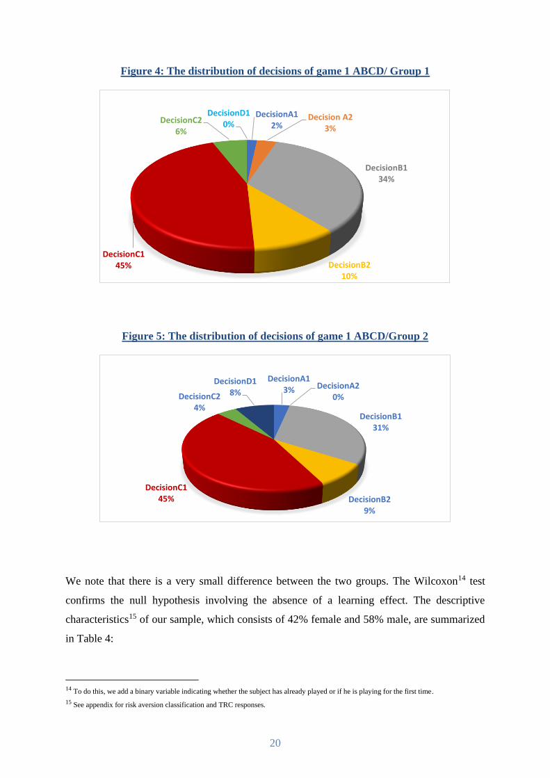
Figure 4: The distribution of decisions of game 1 ABCD/ Group 1
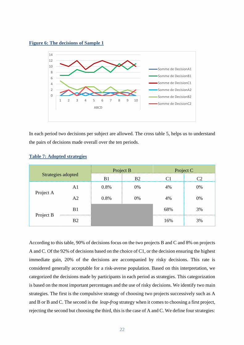
Figure 5: The distribution of decisions of game 1 ABCD/Group 2
We note that there is a very small difference between the two groups. The Wilcoxon14 test
confirms the null hypothesis involving the absence of a learning effect. The descriptive
characteristics15 of our sample, which consists of 42% female and 58% male, are summarized
in Table 4:
14 To do this, we add a binary variable indicating whether the subject has already played or if he is playing for the first time.
15 See appendix for risk aversion classification and TRC responses.
DecisionA12%
Decision A23%
DecisionB134%
DecisionB210%
DecisionC145%
DecisionC26%
DecisionD10%
DecisionA13% DecisionA2
0%
DecisionB131%
DecisionB29%
DecisionC145%
DecisionC24%
DecisionD18%

21
Table 6: Sample descriptive statistics
This table shows that the population studied is on average risk-averse and has a tendency to use
system 1. This system in most cases provides quick and non-correct intuitive answers, rather
than thought-provoking analytical answers. It should be noted that only 8% give three correct
answers and 92% give at least one wrong answer. Frederick's (2005) study of a population of
more than 3,000 Americans shows that 17% correctly answer the three TRC questions. De Neys
et al (2013) find that 83% of subjects providing false answers to the first TRC question had
total confidence in having correct answers. Regarding the AR variable, 8% are risk-seekings.
The choices of this population over the ten periods are shown in Chart 5. A careful observation
of this graph reveals the following information summarized in Figure 6.16
Decisions B1 and C1 are the most preferred for most subjects. While decisions are stable, other
decisions have two different levels depending on whether one is at the beginning or the end of
the period. The choice of C1 is relatively stable over the ten periods. On the other hand, the
choice of B1, which did not attract the interest of most decisions at the beginning of the first
and second period, ended up joining the values reached by the choice of C1. This phenomenon
is known to experimental economists as the "end effect". This effect is defined as the change in
subject behavior between the first and last periods. During these early periods, some
participants tended to make risky decisions, which explain the evolution of the B2 curve. This
decision, in contrast to decision B1, is on a downward trend at the end of the period. The choice
of other A1, A2 and C2 decisions remains very limited, stable and sometimes takes zero value
in certain periods.
16 The choice of decision D1 is negligible over the ten periods compared to a total of 120 decisions and therefore strategies based on the
adoption of old technologies are not included in our experimental results. We then neglected Project D, which only takes one period (which
allows us to focus on two-period projects)
Variable | Obs Mean Std. Dev. Min Max
------------- + ---------------------------------------------------------
TRC | 12 0.75 0.9251756 0 3
AR | 12 6.25 1.480563 3 9
22
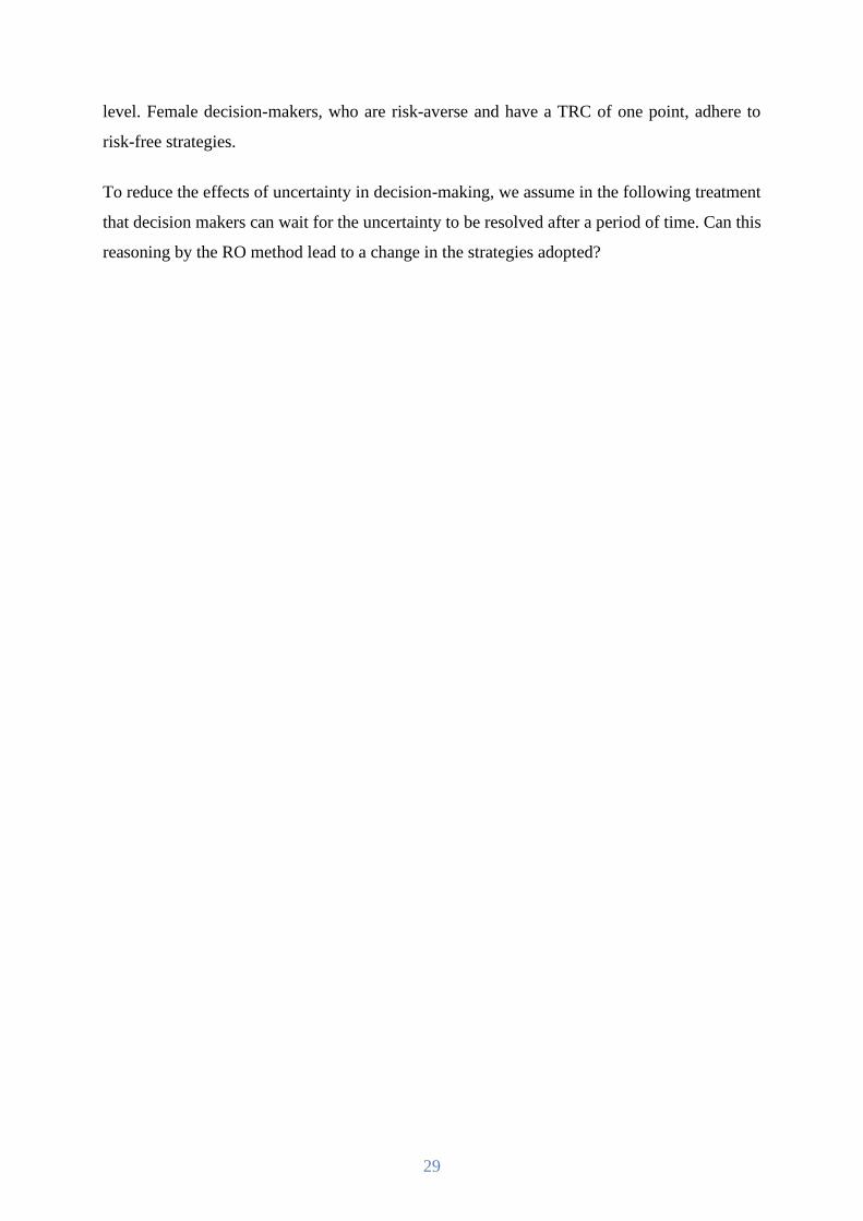
Figure 6: The decisions of Sample 1
In each period two decisions per subject are allowed. The cross table 5, helps us to understand
the pairs of decisions made overall over the ten periods.
Table 7: Adopted strategies
Strategies adopted Project B Project C
B1 B2 C1 C2
Project A A1 0.8% 0% 4% 0%
A2 0.8% 0% 4% 0%
Project B
B1
68% 3%
B2 16% 3%
According to this table, 90% of decisions focus on the two projects B and C and 8% on projects
A and C. Of the 92% of decisions based on the choice of C1, or the decision ensuring the highest
immediate gain, 20% of the decisions are accompanied by risky decisions. This rate is
considered generally acceptable for a risk-averse population. Based on this interpretation, we
categorized the decisions made by participants in each period as strategies. This categorization
is based on the most important percentages and the use of risky decisions. We identify two main
strategies. The first is the compulsive strategy of choosing two projects successively such as A
and B or B and C. The second is the leap-frog strategy when it comes to choosing a first project,
rejecting the second but choosing the third, this is the case of A and C. We define four strategies:
0
2
4
6
8
10
12
14
1 2 3 4 5 6 7 8 9 10
ABCD
Somme de DecisionA1
Somme de DecisionB1
Somme de DecisionC1
Somme de DecisionA2
Somme de DecisionB2
Somme de DecisionC2

23
• The leap-frog strategy (rated StrgLf1): corresponds to the choices of projects A and C.
In this case, we focus on the "A2-C1" decisions. On the one hand this strategy contains
a risky decision and on the other hand the choice of A1 is negligible along the 1ABCD
game.17
• The risk-free compulsive strategy (rated StrgCp0): corresponds to the choices of
projects B and C in their early phases. In other words, these are the "B1-C1" decisions.
This strategy accounts for 68% of participants' decisions over the ten periods.
• The compulsive strategy with a risky project (rated StrgCp1): corresponds to the choices
of projects B and C, but with the decisions "B2-C1" or "B1-C2". This strategy ranks as
the second most chosen strategy and contains a risky project.
• The compulsive strategy with two risky projects (rated StrgCp2): corresponds to the
choices of projects B and C but with two risky decisions that are "B2-C2", hence its
peculiarity.
To understand the behavioral characteristics of the choices of these strategies, we opted for an
econometric estimate. Each strategy is then equated with a binary variable taking value 1 if
adopted and value 0 if it is not. Our experimental data is characterized on the one hand by a
binary dependent variable and on the other hand players are led to decide between several
choices over ten periods. The appropriate model for these characteristics is mixed-effect logistic
regression in panel data. Mixed logistic regression is also seen as an extension of generalized
linear models to include both fixed and random effects (i.e. mixed models). In the case of panel
data the integration of the random effect is very important to avoid the problems of self-
correction and take into account the different sources of variability. The peculiarity of this
method of regression stems from its ability to take into account the different distributions other
than Gaussian distribution; such is our case of binary logistic distribution. We briefly outline
his formulation assumptions. The method is based on the introduction of a function known as
the "link". By posing that there is a linear predictor noted 18η which is the combination of fixed
and random effects excluding residues:𝜀
η = Xβ + Zu
17 The values used (0.1.2) in policy abbreviations indicate the number of risky projects for any strategy. 18 To see Vermunt (2005) and Rabe-Hesketh And Skrondal (2012) for more analytical details on the model. Econometric estimates are made
on Stata 16.0 software.

24
And by posing that there is a function 𝑔(. )called a link function that connects the dependent
binary variable involving the predictor 𝑝 = 𝑃(𝑌 = 1)η, then the conditional expectation of our
model is:
𝑔[𝐸(𝑌)] = η
⟹ 𝐸(𝑌) = 𝑔−1(η) = μ
And of course: 𝑌 = 𝜇 + 𝜀 . Our link function is therefore the logistic function where Y and u
follow Bernoulli's law of expectation 𝑝:
𝑙𝑜𝑔𝑖𝑡(𝑝) = 𝑔(𝑝) = 𝑙𝑛𝑝
1 − 𝑝= η ⟹ 𝑌∗ = 𝜇 + 𝜀
⟹ 𝑔−1 =𝑝
1 − 𝑝= 𝑒η ⟹ 𝑝 =
𝑒η
1 + 𝑒η
The quantity 𝑝
1−𝑝 defines what is commonly called "odds ratio", in other words a chance ratio
and so 𝑌∗ is a latent variable. Thus, in our first estimate in panel data we assume 𝑝𝑖𝑡 =
𝑃(𝑌𝑖𝑡 = 1): which refers to the probability of choosing the compulsive strategy by an individual
i at the period t. The Likert scale at least risk-seeking at most risk-averse is used to assess the
independent variable of risk aversion (RA). For the Cognitive Reflection Test (CRT), it is
evaluated based on the number of correct responses. The estimate of this method in Table 6
shows that behavioral and gender variables significantly affect the decision to adopt the risk-
free compulsive strategy. While the choice of this strategy increases with risk aversion, it
decreases with the increase in test score of cognitive and female gender thinking. Although
results on risk aversion and CRT are expected, such results do not support the majority of
findings. In other words, it is women's decision-makers who prefer non-risky decisions more.
Montmarquette (2008) suggests that in order to decide such a debate, which is not the objective
of our study, sessions with similar participants were required.

25
Table 8: Results of regression 1
Table 6 also shows a regression such that the compulsive strategy with a single risky project is
the dependent variable. This estimate shows a reversal of the signs of the explanatory variables.
The results also confirm that risk aversion is an important determinant that negatively affects
risky decisions. Indeed, the investment in risky activity decreases significantly with the degree
of risk aversion of the individual. However, it increases with the level of CRT and when the
decision-makers are more likely to be women. Although the decisions of StrgCp1 do not exceed
19%, the estimate is of significant significance. This allows us to compare the effects of the
variation of independent variables on the two strategies.
However, as explained above in the non-linear logistic regression model, it is difficult to
interpret the coefficients of the explanatory variables. Indeed, the dependent variable is a latent
variable: it is the logarithm of "odds". What we want to see for interpretation are the effects on
results such as probabilities (which measure the degree of certainty of the realization of an
event) and not on the "odds ratio". To do this, we move on to the analysis of marginal effects.
This analysis shows, from Tables 7 and 8, that a subject with a single correct TRC answer has

26
a 20% chance of choosing compulsive strategy with a risky project, compared to 66% for
choosing the risk-free compulsive strategy. When all TRC responses are correct, the probability
of opting for a strategy containing a risky project will reach 40%. On the other hand, it is the
risk-seekings, only, who have a 40% chance to opt for the said strategy. This probability
increases to 10% for high-risk-averse individuals, while 78% decide for a non-risky compulsive
strategy.
Table 9: Marginal effects for the dependent variable: StrgCp0
This econometric study shows the importance of the explanatory variables chosen for decisions
in an uncertain environment. In fact, several questions arise as a result of this estimate. Are all
the decisions of the risk-averse far from containing a certain level of risk? What about a risk-
averse decision but with a high CRR score or what about a risk-averse decision maker but with
a low CRR score. In our sample, the gender variable is significant; can we say that regardless
of their RA and CRT, women tend to be in favor of an uncertain decision?
Table 10: Marginal Effects for the Dependent Variable StrgCp1

27
To deepen our analysis, we propose an attempt to classify our sample by applying the ID3
algorithm, which is widely used in the field of "Data mining". With this algorithm we aim to
partition our sample into groups, as homogeneous as possible, in the form of a tree. To build
such a tree, we usually start with the choice of an attribute and then the choice of a number of
criteria for its node. For each criterion, we create a node for the data that verifies that criterion.
The algorithm continues recursively until the nodes of the data of each class are completed.
This algorithm uses the concepts of entropy and information gain to choose the nodes of the
decision tree. The most well-known entropy is Shannon's. It first defines the amount of
information provided by an event: the lower the probability of an event, the greater the amount
of information it brings. Thus, entropy E for a given set is calculated on the basis of the
classification of the class of the fixed samples. The information gain is calculated by the
following formula:19
𝐺(𝐷, 𝐴) = 𝐸(𝐷) − 𝐼(𝐷, 𝐴)
With: 𝐸(𝐷) = − ∑ 𝑝𝑖𝑙𝑜𝑔2(𝑝𝑖)𝑘𝑖=1
19 See Andrew Oleksy (2018)
6 .4007686 .120151 3.34 0.001 .1652769 .6362603
5 .297026 .0642996 4.62 0.000 .1710011 .423051
4 .2094254 .0343086 6.10 0.000 .1421819 .276669
3 .1023877 .0310153 3.30 0.001 .0415988 .1631765
2 .2525976 .0361215 6.99 0.000 .1818008 .3233945
1 .4055196 .0367938 11.02 0.000 .333405 .4776342
_at
Margin Std. Err. z P>|z| [95% Conf. Interval]
Delta-method
6._at : TRC = 3
5._at : TRC = 2
4._at : TRC = 1
3._at : AR = 8
2._at : AR = 5
1._at : AR = 3
Expression : Predicted mean, predict()
Model VCE : OIM
Predictive margins Number of obs = 120
. margins, at(AR=(3 5 8)) at(TRC=(1 2 3))

28
𝐼(𝐷, 𝐴) = ∑|𝐷𝑗|
|𝐷|𝐸(𝐷𝑗)
𝑗
In our case, since a good majority of the decisions taken were in favor of the absence of
uncertainty, the classification is to divide decision-makers, either as risk-taking decision-
makers (regardless of number of risky projects) that are noted DR1, or as non-risk decision-
makers (with zero risky projects) that are noted DR0. So D is represented by either DR1 or
DR0. The probability of class i in D is noted by 𝑝𝑖. |𝐷𝑗| represents the number of j value cases
for feature A. |𝐷| refers to the number of all cases. 𝐸(𝐷𝑗) is entropy for the subset of the entire
dataset having the j value for feature A. Our data results are:
Table 11: Applying the ID3 algorithm
𝑬(𝑫) 𝑰(𝑫, 𝑨) 𝑮(𝑫, 𝑨)
A=AR 1 0.42 0.58
A=TRC 1 0.8 0.2
A=Gender 1 0.98 0.02
We note from Table 9 that the risk aversion variable reports the highest information gain.
Therefore, it appears as the root of our decision tree. We then build the branches of the tree
according to the different values of the root variable. The D data set is divided into as many
subsets as the discrete values of the chosen variable. For each subset must correspond to it a
single value of the D class and that represents the sheet. The values for which the assignment
of a decision is impossible, we take up the calculations of the information gains for the
remaining variables. This process stops until it is no longer possible to create leaves.
The tree shown in Figure 7 summarizes the characteristics of our sample. They show that all
those who are risk-seeking make risky decisions in most cases regardless of their CRTs.
However, for those who are risk-averse, it is their CRT scores that will determine their
involvement in strategies characterized by the absence of uncertainty. When decision-makers
are both, either risk-averse, risk-averse or very risk-averse, and have a CRT of at least one
point, they do approve of risky choices. Only the highly risk-averse make the least uncertain
decisions even with low gains. They also reveal that the gender variable only occurs at the last
29
level. Female decision-makers, who are risk-averse and have a TRC of one point, adhere to
risk-free strategies.
To reduce the effects of uncertainty in decision-making, we assume in the following treatment
that decision makers can wait for the uncertainty to be resolved after a period of time. Can this
reasoning by the RO method lead to a change in the strategies adopted?

30
Figure 7: Applying the ID3 algorithm on decision-making
3 8
5 6 7 TRC 2-3-1
1 0
1 0
M F
AR

31
II-1-c- The choice of two projects between four projects with waiting
We wonder in this treatment if the introduction of the wait can affect the strategies of the
players. Always with the constraint of choosing two projects, participants, unlike the first
treatments, can see the result of the coin toss and then they make the decision whether to adopt
the project.
Result 3: The OR approach strengthens the leap-frog strategy and therefore increases the gain.
Those who opt for the compulsive strategy are the risk-averse. Risk-seeking decision-makers
tend to adopt the leap-frog strategy.
Support 3: Comparison of Figure 8 with the two Figures 4 and 5 shows stability in decisions
A1, B2 and C2 against a very significant increase in the choice of decision A2. The choice of
this decision goes back to 21% at the expense of decision B1 and C1. Although their shares,
over the ten periods and for all participants, would still occupy the front rows. In addition we
notice that all participants accepted project A2 when the positive gain. This mutation
necessarily implies a new distribution of different strategies.
Figure 8: The distribution of decisions with expectation
Table 10, compared to table 5, shows a marked increase in adoptions of strategies containing
one or two risky projects. In fact, it is the wait-and-see strategy that can make risky decisions
more apprehensive, resulting in a more controlled flexibility in accepting or rejecting projects.
Somme de DecisionA1
3%
Somme de DecisionA2
21%
Somme de DecisionB1
25%Somme de DecisionB2
7%
Somme de DecisionC1
39%
Somme de DecisionC2
5%

32
Table 12: The breakdown of the different strategies adopted
Strategies adopted Project B Project C
B1 B2 C1 C2
Project A A1 3% 0% 3% 0%
A2 5% 3% 28% 5%
Project B B1 40% 2%
B2 7% 3%
Figure 9 describes the evolution of the choice of different strategies over the ten periods.
Individuals have a tendency to take the risk just in the early periods which explains the increase
in the adoption of the leap-frog strategy. Rather, the end-of-period phenomenon is characterized
by the dominance of risk-free compulsive strategy. It seems that this phenomenon (already
existing in the previous game) is independent of the behavioral characteristics of the subjects.
Compared to the previous sample, our sample in this treatment is more homogeneous with AR,
but with a higher CRT as shown in table 11.
Figure 9: The evolution of different strategies over ten periods
Estimates have already been made that we can predict greater recourse to strategies that contain
risky decisions, particularly because this uncertainty is partly resolved. Compared to the
GW(1997) model, the dominant strategies are: first, the compulsive strategy and second, the
leap-frogstrategy. Members of the leap-frog strategy on one or two risky projects have a risk
aversion of between 0.68 and 0.97 and have an average of 1 higher CRT.

33
Table 13: Descriptive statistics on RA and CRT for different strategies.
For the following econometric estimate, we opted for the panel-data-mixed-logit-choice model.
This model allows us to understand the choice of different strategies as a whole or in relation
to a basic alternative (strategy). Mixed logit models have the distinction of using random
coefficients to model the correlation of choices between alternatives. These random coefficients
allow us to relax the independence of the irrelevant alternative hypothesis that is required by
some other choice models. In addition, 20the use of the mixed-effect logit model in panel data
allows us to model the probability of selecting each alternative for each period rather than
modeling a single probability to select each alternative (which is the case with cross-sectional
data).
The results of table 12 significantly confirm the previous estimate for RA and CRT. An increase
in CRT makes it more likely to choose riskier strategies either for compulsive or leap-frog
strategies, rather than certain compulsive strategy. Conversely, an increase in RA makes it less
likely that decisions are made uncertain, but of course encourages the implementation of a risk-
free compulsive strategy. For leap-frog1strategy, the gender variable is positive, ensuring that
female gender individuals are more likely to choose or proceed with such a strategy, rather than
to compulsive strategy without risk.
20 For more technical details see Han et al (2020).
Total 7.354167 1.3125
StrgLp2(A2C2) 7.333333 1.666667
StrgLp1(A2C1) 7.058824 1.588235
StrgCp1(B2C1) 8 1.75
StrgCp0(B1C1) 7.458333 1
_chosen_alternative AR TRC

34
Table 14: Econometric estimate of "Choice Models"
Post-estimate predictions show that, depending on the characteristics of our sample, 48% opt
for the certain compulsive strategy and 36% opt for the leap-frog strategy according to the
approach by the actual options. Compulsive strategy1 and leap-frog2 strategy benefited by
8.7% and 6.5% respectively.
When all decision-makers are women, the choice of certain compulsive strategy represents 42%
versus 58% when all decision makers are male. The latter choose the leap-frog strategy only in
15% of cases, while this same strategy will have a 48% probability of being adopted if all
decision makers are women. However, predictions show that the riskiest B2C1 compulsive
strategy, which at the same time can provide a significant gain over other strategies, represents
a 19% probability for male decision-makers, compared to 3% for female decision-makers.
Figure 10 shows that the increase in RA increases the adoption of the compulsive strategy by
53% for risk-averse individuals, but it decreases the adoption of the leap-frog strategy. Risk-
seekings choose this strategy in 58% of cases. Thus, we confirm the theoretical findings put
forward by Chronopoulos and Lumbreras (2016) and Alexander and Chen (2019).
Genre1F .4298158 1.248899 0.34 0.731 -2.017982 2.877613
TRC 2.348121 1.190289 1.97 0.049 .0151975 4.681044
AR -.7072021 .2654694 -2.66 0.008 -1.227512 -.1868917
StrgLp2_A2C2_
Genre1F 1.768588 .8630271 2.05 0.040 .0770856 3.46009
TRC 2.342811 .8513193 2.75 0.006 .6742558 4.011366
AR -.6042621 .1839182 -3.29 0.001 -.9647352 -.2437889
StrgLp1_A2C1_
Genre1F -1.14717 1.280401 -0.90 0.370 -3.656709 1.362369
TRC 2.376362 1.149509 2.07 0.039 .1233664 4.629358
AR -.5807847 .2419698 -2.40 0.016 -1.055037 -.1065325
StrgCp1_B2C1_
StrgCp0_B1C1_ (base alternative)
decision Coef. Std. Err. z P>|z| [95% Conf. Interval]
Log likelihood = -41.176045 Prob > chi2 = 0.0003
Integration points: 0 Wald chi2(9) = 30.64

35
Figure 10: Prediction between the evolution of RA and different strategies
Conversely, this strategy is in increasing relation to the CRT. Those with the highest CRT value
choose this strategy with a 65% probability.
Figure 11: The effect of CRT variation on different strategies
To conclude this first part, we can say that in the absence of a competitor in the market, the
subjects choose to adopt, in most cases, projects with relatively large values, some and
immediate. They project the expectation or practice of the method by the actual options for
projects with low immediate values (with the aim of increasing their values). Thus, it seems
that the real options approach promotes the leap-frog strategy that increases the gain by
36
minimizing uncertainty. The RA itself is not a constraint for the choice of risky projects unless
it is coupled with a zero CRT.
II-2-Analysis of results of game 2
To configure the effect of competition on the adoption of new technologies as part of the real
options approach, we consider that the decision made by one individual is affected by the
decision of another individual. Their decisions are thus made simultaneously. We are drawing
a competition of the monopoly; each group is then composed of two students. Students play in
"strangers" mode where group members change after each period randomly. Compared to the
"partners" mode whereby each group keeps the same members during all periods of the
experiment, Weimann (1994) shows that "partners" and "strangers" generally behave
similarly. Below we first show the results of the 2A, 2B and 2C games. Secondly, we analyze
the results of the game 2AB and the game 2ABC.
II-2-a-Results of games 2A, 2B and 2C
During this treatment, the subjects were randomly matched with another participant and were
asked to choose either "adopt" or "wait". In other words, both subjects are in a position to invest
now, but they also have the option of deferring investment. We note that all participants are
informed about the underlying assumptions and values, as well as financial incentives prior to
the launch of the investment experience. However, to keep the information asymmetry
hypothesis, subjects were not informed of the other person's choice prior to decision-making. It
also reflects the idea that the company will make the decision without knowing what other
companies will do and how they will react to its decision to invest.
In this context, we have developed two types of the game. The first game, 2A, is a simple stable
Nash balance game. The second type of games, 2B and 2C, are two games of the prisoner
dilemma.
Thus, the increase in the value of projects on the three treatments (2A, 2B and 2C) allows us to
assess the effect of such an increase on the decision of subjects in other words on the waiting
strategy. Thirty students played the 2A, 2B and 2C games. A first group of fourteen students,
played in "strangers" mode and a second group of sixteen students, played in "partners" mode.
We note that the subjects were not informed of the nature of the relationship with the other
player.

37
II-2-a-i- Game 2A Results
This first game, 2A, is a simple stable Nash balance game. In this game, theoretically speaking,
none of the players has a motivation to deviate from the situation of balance. This scenario
appears to be a coordinated strategy. Recalling, as we have already explained, that in this case,
two situations of equilibrium arise: either (adopt, adopt) or (wait, wait). However, it is clear that
the balance of expectation ensures more profit for both companies. In fact, can we expect such
a result?
Regardless of the validity of Nash's equilibrium, we confirm Holt&Roth (2005) postulate: " The
Nash equilibrium is useful not just when it is itself an accurate predictor of how people will
behave in a game but also when it is not, because then it identifies situations in which there is
a tension between individual incentives and other motivations".
Result 4: The waiting strategy representing the stable Nash balance is not experimentally
verified. The pre-emption game dominates from the fifth period. Assumption 6 is not verified.
Support 4: It is clear from the observation of figures 12 and 13 that the maximum value of the
choice of the waiting strategy peaked at 75% in the first period for the G2. This group that
played in "partner" mode shows a waiting rate, on average 54%, significantly higher than the
G1 with an average of 41%. While the decisions of both groups diverged in the first, second
and seventh periods, both treatments experienced their lowest levels towards the end of the
period. The G1 boxplot shows instability (distribution is more extensive) in making the waiting
decision, in contrast to G2 decisions where decisions were more stable. Generally, in the
majority of experiences and regardless of the mode of the game, individuals have a tendency to
start by seeing if cooperation is possible. The G2 subjects sought this cooperation from the first
period, while the G1 participants sought it a little later, in the third period. Often, individuals
avoid starting a repeated game with uncooperative behavior in order not to jeopardize the
chances of possible cooperation during the remaining periods of the game. However, at the end
of the game we move further and further away from Nash's balance, even if Nash's balance is
dominant. The fact that the subjects' decisions are different from Nash's balance revives the
idea that experimental results do not verify theoretical predictions. These are therefore called
into question and new explanations are advanced by the experimental method. This deviation
from balance raises the question of the rationality of individuals. Waiting or adopting
immediately is directly related to the risk aversion of the subjects. The waiter takes the risk of
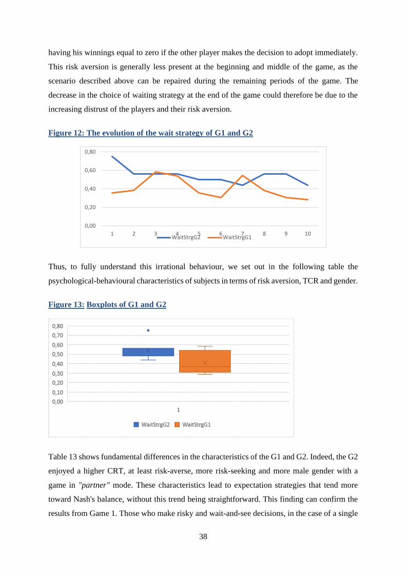
38
having his winnings equal to zero if the other player makes the decision to adopt immediately.
This risk aversion is generally less present at the beginning and middle of the game, as the
scenario described above can be repaired during the remaining periods of the game. The
decrease in the choice of waiting strategy at the end of the game could therefore be due to the
increasing distrust of the players and their risk aversion.
Figure 12: The evolution of the wait strategy of G1 and G2
Thus, to fully understand this irrational behaviour, we set out in the following table the
psychological-behavioural characteristics of subjects in terms of risk aversion, TCR and gender.
Figure 13: Boxplots of G1 and G2
Table 13 shows fundamental differences in the characteristics of the G1 and G2. Indeed, the G2
enjoyed a higher CRT, at least risk-averse, more risk-seeking and more male gender with a
game in "partner" mode. These characteristics lead to expectation strategies that tend more
toward Nash's balance, without this trend being straightforward. This finding can confirm the
results from Game 1. Those who make risky and wait-and-see decisions, in the case of a single
0,00
0,20
0,40
0,60
0,80
1 2 3 4 5 6 7 8 9 10WaitStrgG2 WaitStrgG1

39
decision maker, are either risk-seeking or risk-averse with at least one correct answer. It is also
those who decide to opt for the waiting strategy when it is a dominant strategy.
Table 15: The behavioral characteristics of G1 and G2
Group 1 Group 2 Group 3
Kind Female 50% 31% 75%
Masculin 50% 69% 25%
TRC
0 correct answer 79% 25% 41.5%
1 correct answer 14% 62.5% 41.5%
2 correct answers 0% 0% 17%
3 correct answers 7% 12.5% 0%
Ar21
Risk-seeking 14% 25% 8%
Risk neutral 21% 25% 8%
Risk-averse 65% 50% 84%
It also turns out, however, that risk-averse with zero CRT have rather aggressive competitive
behavior resulting, in most cases, in balance (Adopt, Adopter) and thus achieving the lowest
gain. We then use a group behavior analysis that could clarify the details of this outcome.
Since the G1 has played in "stranger"mode, it is therefore impossible to report the decisions of
these days. We represent in the graph following the G2, whose participants played "partner".
Figure 14: The evolution of the different gains of the subgroups G2 over ten periods
21 HL - 0-3: risk-seekings, HLL - 4: risk neutral, HLL - 5-10: risk-averse ( Holt and Laury (2002))

40
To represent this graph, we have opted for the following procedure:
− Value 3 represents the gain when both individuals in the same group opt for the immediate adoption
strategy.
− Value 6 represents the gain when one of the two individuals in the same group opts to adopt immediately,
while the other opts for waiting.
− Value 8 represents the gain when the two individuals in the same group decide to wait.
Figure 14 shows three types of subgroups in the G2:
▪ Groups 2.2, 2.3, 2.4, 2.5 and 2.6 started the game with the waiting strategy. However, it
is groups 2.2, 2.4 and 2.6 that check Nash's stable balance over the ten periods. These
groups consist of couples who are both risk-seeking or a risk-averse and has a CRT with
one or three correct answers. This observation confirms at least in part our interpretation
above.
▪ While for groups 2.1 and 2.8 only one individual who adopted the waiting strategy
during the first period.
▪ The two subjects in group 2.7 opted for immediate adoption in the first period, and they
kept the same strategy over eight periods, with the exception of periods 3 and 6. Groups
2.1, 2.3 and 2.8 also engage in this aggressive competition and opt in at least 80% of
balanced choices (Adopt, Adopt).
An important question at this level is whether one player's previous strategy will affect the other
player's current decision. To do this, we hypothesize that the mode of the game "partner" or
"stranger" does not have a significant influence on the strategies of the players. For this
purpose of estimation we create a new variable that allows us to take into account the other
0
1
2
3
4
5
6
7
8
9
1 2 3 4 5 6 7 8 9 1 0
G2.1 G2.2 G2.3 G2.4
G2.5 G2.6 G2.7 G2.8

41
player's previous strategy for each group. This variable therefore reflects, for a player, the effect
of an opponent's previous decision on his reaction function in terms of waiting strategy.
Over the ten periods, the evolution of individual choices for the waiting strategy for the thirty
subjects is presented in Figure 15:
Figure 15: The evolution of the waiting strategy
In accordance with the experimental literature in this context, particularly with regard to
cooperation in the game of public goods, the expectation decreases throughout the game. It
starts at 57%, in the first period, on average 46% in rounds 2 to 9, and drops to 37% in the final
period. This decline throughout the game leads us to believe that this learning could exist and
that the ten periods of the game may not be enough to allow players to understand the strategic
outcome of the game. Would the learning process then be a long enough process that requires
a lot of repetition and additional information to be successful?
Econometric analysis of individual behaviors could inform us about this questioning. By
incorporating the two groups of thirty individuals over the ten periods, we get Table 37. While
the signs of variables reflecting aversion and cognitive ability (TRC) confirm the interpretations
already deduced in Games 1 regarding the adoption of the waiting strategy, the sign of the
gender variable is not stable compared to the previous games. The new variable built: "OthStrgt-
1"may reflect the notion of reciprocity.
According to Fehr and Gochter (2000), the founders of behavioral game theory, this reciprocal
behaviour is explained by Fehr and Gochter (2000), that in response to good deeds or
cooperative actions, individuals are often much more cooperative than the conventional model
of self-interest predicts. Conversely, in response to hostile or unfavorable actions, they are often
0
2
4
6
8
10
12
14
16
18
1 2 3 4 5 6 7 8 9 10

42
much more cruel and even aggressive. This description of player behavior allows us the
following inference: remembering that the average rate of adoption of the waiting strategy in
this game could not exceed 46.7% for a stable Nash balance. We can thus conclude that the
minority, who opt for the waiting strategy, ensuring more profit, could not compel the majority
who are in most cases risk-averse or have zero CRTs to choose the right strategy. On the
contrary, in order to join the explanation of Fehr and Gochter (2000), this majority pushed the
minority to be more aggressive.
The most recognized example of this aggressive competition in the monopoly sector is that in
the aviation industry between the two major global companies Boeing and Airbus. Since 2006,
Boeing has been talking about replacing Boeing 737 with a totally innovative design called
"Boeing Y1". The pressure exerted by the airlines, for more energy-intensive aircraft, and the
commissioning of the A320Neo by its competitor Airbus, which was originally scheduled for
mid-2016 and was advanced to October 2015, have prompted Boeing to continue improving
the 737 with new engines rather than embark on the new design of the "Boeing Y1". While
Boeing's Research and Development Program has predicted that the 737 Max will offer 16%
less fuel consumption than the current Airbus A320, and 4% lower than the Airbus A320neo,
the 737 Max has completed two crashes with the death of 346 people.
Table 16: Game 2A regression
On December 16, 2019, Boeing announced that production of the 737 Max would be
discontinued from January 2020. The final report of the U.S. Congressional Transport
Committee "highlights five themes, starting with the strong financial pressure put on Boeing

43
and the 737 Max program to move as quickly as possible in order to better compete with the
Airbus A320Neo. This pressure has prompted Boeing to cut spending and maintain the
production schedule at all costs." In 2019, Airbus replaced Boeing as the largest aerospace
company and the 737 Max crisis has already cost it 22nearly $20 billion.
In this game, with a theoretically stable balance, the adopters of the waiting strategy were
46.7%. What adoption rate can we expect if the game turns into a prisoner's dilemma game?
The following section allows us to resolve this issue.
II-2-a-ii- The Prisoner's Dilemma: Games 2B and 2C
The second type of game is the symmetrical prisoner's dilemma game, with complete and
imperfect information. This type of game, 2B and 2C, illustrate that rational individual
behaviours can go against the collective interest. In fact, this game is a dilemma since on the
one hand, each player would find his interest in an orderly and simultaneous cooperation, but
on the other hand, unilaterally deviating from the latter is profitable, which induces behaviors
of the type stowaway. In Game 2A, the gain from the wait was on the one hand much greater
than the win without expectation if both players decide to adopt immediately and on the other
hand more than the gain of a single player if the other decides to postpone his decision of
adoption. On the other hand, in Game 2C the gain of the wait, if both players decide to wait, is
significantly less than the gain of a single player if he decides to adopt immediately and the
other postpones his decision. This differential of winning in Game 2B is small, but it is more
important than the immediate adoption gain by both players. This characterization helps us to
measure the magnitude of the risk and the degree of claim of the waiting strategy in both games,
according to Rapoport (1967), Au et al (2012).
Result 5-1: the pre-emption strategy is most played especially for projects that are less risky
and by the most risk-averse. This result confirms assumptions 8 and 9.
Result 5-2: the repetition of the DP, for games 2A and 2B, does not induce the game "Tit for
Tat". Assumption 7 is not verified. However, we note that the waiting strategy is more adopted
when the project is riskier and decision makers are less risky.
22*https://www.lemonde.fr/economie/article/2020/09/16/boeing-737-max-le-constructeur-et-le-regulateur-vertement-blames-par-le-congres-
americain_6052451_3234.html *https://fr.wikipedia.org/wiki/Boeing_737_Max#cite_ref-18
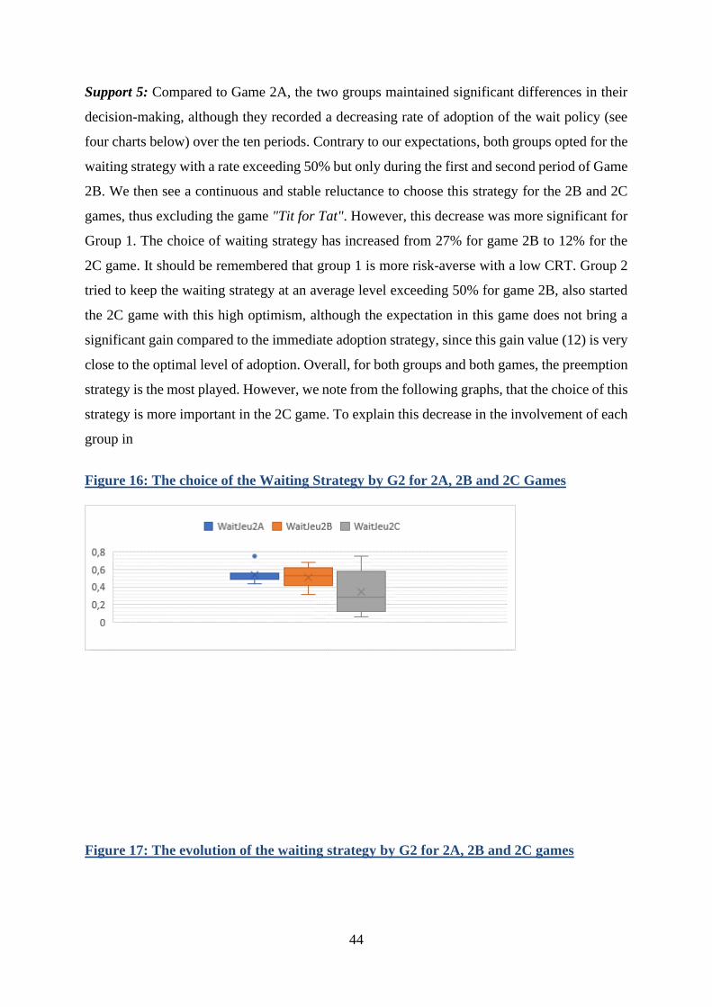
44
Support 5: Compared to Game 2A, the two groups maintained significant differences in their
decision-making, although they recorded a decreasing rate of adoption of the wait policy (see
four charts below) over the ten periods. Contrary to our expectations, both groups opted for the
waiting strategy with a rate exceeding 50% but only during the first and second period of Game
2B. We then see a continuous and stable reluctance to choose this strategy for the 2B and 2C
games, thus excluding the game "Tit for Tat". However, this decrease was more significant for
Group 1. The choice of waiting strategy has increased from 27% for game 2B to 12% for the
2C game. It should be remembered that group 1 is more risk-averse with a low CRT. Group 2
tried to keep the waiting strategy at an average level exceeding 50% for game 2B, also started
the 2C game with this high optimism, although the expectation in this game does not bring a
significant gain compared to the immediate adoption strategy, since this gain value (12) is very
close to the optimal level of adoption. Overall, for both groups and both games, the preemption
strategy is the most played. However, we note from the following graphs, that the choice of this
strategy is more important in the 2C game. To explain this decrease in the involvement of each
group in
Figure 16: The choice of the Waiting Strategy by G2 for 2A, 2B and 2C Games
Figure 17: The evolution of the waiting strategy by G2 for 2A, 2B and 2C games

45
Figure 18: The choice of waiting Strategy by G1 for 2A, 2B and 2C Games
Figure 19: The evolution of the waiting strategy by G1 for 2A, 2B and 2C games
their choices in the two games of the prisoner's dilemma, we use the approach of Ng and Au
(2015) which is based on the classic model of Rapoport (1967) and the coefficient of Au et al.
(2011). According to Repoport, the prisoner's dilemma exists when the values in the table below
verify the following relationship:
Table 17: Repoport's Prisoner Dilemma Table
0
0,2
0,4
0,6
0,8
1 2 3 4 5 6 7 8 9 10
WaitJeu2A WaitJeu2B WaitJeu2C
0,00
0,20
0,40
0,60
0,80
1 2 3 4 5 6 7 8 9 10
WaitJeu2A WaitJeu2B WaitJeu2C
0.2
0.4
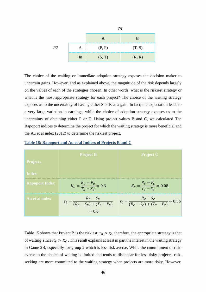
46
P1
A In
P2 A (P, P) (T, S)
In (S, T) (R, R)
The choice of the waiting or immediate adoption strategy exposes the decision maker to
uncertain gains. However, and as explained above, the magnitude of the risk depends largely
on the values of each of the strategies chosen. In other words, what is the riskiest strategy or
what is the most appropriate strategy for each project? The choice of the waiting strategy
exposes us to the uncertainty of having either S or R as a gain. In fact, the expectation leads to
a very large variation in earnings, while the choice of adoption strategy exposes us to the
uncertainty of obtaining either P or T. Using project values B and C, we calculated The
Rapoport indices to determine the project for which the waiting strategy is more beneficial and
the Au et al index (2012) to determine the riskiest project.
Table 18: Rapoport and Au et al Indices of Projects B and C
Projects
Index
Project B Project C
Rapoport Index 𝐾𝐵 =
𝑅𝐵 − 𝑃𝐵
𝑇𝐵 − 𝑆𝐵= 0.3 𝐾𝐶 =
𝑅𝐶 − 𝑃𝐶
𝑇𝐶 − 𝑆𝐶= 0.08
Au et al index 𝑟𝐵 =
𝑅𝐵 − 𝑆𝐵
(𝑅𝐵 − 𝑆𝐵) + (𝑇𝐵 − 𝑃𝐵)
≈ 0.6
𝑟𝐶 =𝑅𝐶 − 𝑆𝐶
(𝑅𝐶 − 𝑆𝐶) + (𝑇𝐶 − 𝑃𝐶)≈ 0.56
Table 15 shows that Project B is the riskiest: 𝑟𝐵 > 𝑟𝐶, therefore, the appropriate strategy is that
of waiting since 𝐾𝐵 > 𝐾𝐶 . This result explains at least in part the interest in the waiting strategy
in Game 2B, especially for group 2 which is less risk-averse. While the commitment of risk-
averse to the choice of waiting is limited and tends to disappear for less risky projects, risk-
seeking are more committed to the waiting strategy when projects are more risky. However,

47
they are experiencing a significant and rapid decline in the choice for Project C, which is less
risky. This behavior could be a revision of the strategies played or learning over time. Players
are led to understand that their dominant strategy is to adopt immediately, avoiding on the one
hand having a zero gain and thus achieving a gain close to the optimal situation (for the game
2C).
Games 2A, 2B and 2C study the behavior of competitors when it comes to investing or
postponing adoption in the presence of a single NT. With the increase in the number of projects
available, can we expect a further deterioration or a strengthening in the choice of the waiting
strategy? Can the FM and SM structure be foreseen or rather a more aggressive competition
structure such as the "war of attrition"?
II-2-b-Results of 2AB and 2ABC
Through the 2AB and 2ABC games, we want to study the behavior of competitors when two
or three NT are available respectively. In the DP game, in the presence of an NT, companies
are much more forced to choose immediately to avoid zero profit. In fact, several sectors, such
as the ICT sector, are characterized by a rapid rate of the emergence of NT. All companies in
this case have more likelihood or chance to make positive profits. The values of these two
games partly reflect the tree in Figure 28 but with the existence of two projects and eliminating
the possibility of rejection over both periods. The player, taking into account the behavior of
his partner must decide only to buy a single project, either immediately or while waiting for the
second period. Each player can understand the other's decision by observing their winnings for
each choice. In this game (also the game 2ABC), the subjects play both simultaneously and
sequentially. In other words, when making a decision about Project A, no player can see the
other's decision. Once the choices are made, each player can see on the screen the decision of
the other. This is a non-zero-sum game where each company can improve its profit without
ousting the other's profit. Participants in these games are G2 subjects who have previously
played 2A, 2B and 2C and twelve other topics that we call G3. The latter group started the 2AB
game directly and they played the "partner" mode for the 2AB game, which makes it easier for
us to compare the results of the two groups and the evolution of their decisions over the ten
periods. For the game 2ABC, the same group played in "stranger" mode.

48
II-2-b-i- 2AB Game Result
While in the DP game, no player has the opportunity to take advantage of the observation of
the behavior of his competitor, in this game such luck may exist. Is it possible, therefore, to
achieve a new, less aggressive competition structure? What behaviour can arise if the number
of available technologies increases?
Result 6: when the number of technology available increases the choice of waiting strategy can
reach more than 70% on average. The deviation from the waiting strategy does not appear to
be beneficial.
Support 6: The choice of the immediate adoption strategy, whether for Project A or B, does not
expose its decision maker to the risk of zero profit. However, the choice of the waiting strategy
locks up such a risk but with a lower probability than the DP. The choice of waiting strategy
was well maintained over the ten periods and there was no end-of-period phenomenon of
previous games. In this game, the subject who decides to postpone his investment and wait will
be able to observe what others will do. This will give him the advantage of having more
information on which to base his decision. The characteristics of the subjects of both groups
are summarized in Table 12. Group 3 is more risk-averse, with a low TRC below group 2 and
with more female subjects. Figures 20 and 21 represent the results of the decisions of both
groups. Because the results of the two groups are not different, we can see that group 2 has not
experienced a learning effect.
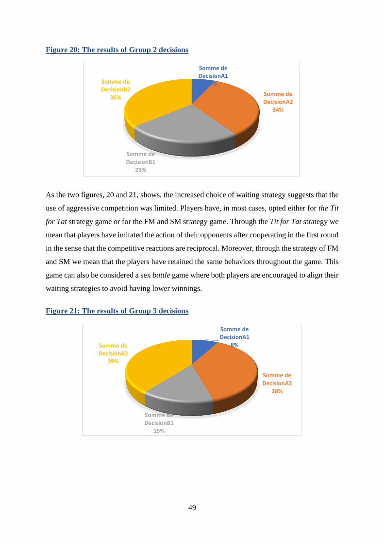
49
Figure 20: The results of Group 2 decisions
As the two figures, 20 and 21, shows, the increased choice of waiting strategy suggests that the
use of aggressive competition was limited. Players have, in most cases, opted either for the Tit
for Tat strategy game or for the FM and SM strategy game. Through the Tit for Tat strategy we
mean that players have imitated the action of their opponents after cooperating in the first round
in the sense that the competitive reactions are reciprocal. Moreover, through the strategy of FM
and SM we mean that the players have retained the same behaviors throughout the game. This
game can also be considered a sex battle game where both players are encouraged to align their
waiting strategies to avoid having lower winnings.
Figure 21: The results of Group 3 decisions
Somme de DecisionA1
7%
Somme de DecisionA2
34%
Somme de DecisionB1
23%
Somme de DecisionB2
36%
Somme de DecisionA1
8%
Somme de DecisionA2
38%
Somme de DecisionB1
15%
Somme de DecisionB2
39%

50
Result 7: the waiting strategy arises in the FM and SM games: each company enjoyed a profit
from the monopoly. This result confirms hypothesis 10. Thus the two results 5-1 and 7 check
cases 1 and 2 of the Model Huissman and Kort (2004).
Support 7: To demonstrate this result, we define the following strategies associated with the
different decisions made by each subject at the fourteen group level over the ten periods since
the groups are in "partner" mode:
• SvStrg: This strategy, which we call a rescue, occurs when both players reject Project
A and both decide to immediately adopt Project B to avoid a possible cancellation of
the gain of one of the days.
• AgrStrg: This strategy, which we describe as aggressive, is the opposite of the previous
strategy. The gain of one of the players, when Project A is not adopted, is necessarily
zero. The game, according to this strategy, appears as a game of war of attrition where
each company must decide to reduce its losses and exit, or to solve it in the hope that
the competitor will leave the market soon.
• TTStrg: This strategy is an attempt to request the cooperation or play of Tit for Tat
following an aggressive strategy.
• FmsmStrg: This FM and SM strategy usually occurs as a result of the TTStrg strategy
and one player maintains to have the highest gain, resulting from the B2 decision, and
the other player accepts the winning of the A2 decision several times. In most cases,
this game continues until the tenth period. We call FM the one who makes the decision
B2.
Figure 22: boxplots for different strategies

51
Overall, the dominant strategy of FM and SM took the largest share of 53%, and then it is the
strategy announcing a possible game of Tit for Tat with 27%. The aggressive strategy is the
latest with a rate of 9% that is not far enough from the 11% rescue strategy. Over the ten
periods, each subject has on average the chance to play seven times the strategy of FM and SM,
while he can propose cooperation three times and only or fortunately he can play only once,
fortunately, aggressive strategy or rescue.
With more detail, Figure 23 represents the evolution of these strategies for the fourteen groups
over the ten periods. The first period is characterized by two dominant strategies. Knowing that
50% of the players began to offer their optimism of the game Tit for Tat, while 40% opted for
the immediate adoption of Project B. Only 10% of the players chose the aggressive strategy
that has also disappeared during the last three periods. As the game repeats itself, SvStrg and
TTStrg's strategies are transformed into FM and SM strategies. Some players maintained their
choices for decision B2 which forced their partners to reject the proposals for the change of role
and accept a lower but certain gain. It was this behavior that made the game of FM and SM
appear, whose curve has seen a steady increase over the ten periods. While two groups still
refused to align with their opponents, this strategy was the choice of twelve out of fourteen
groups in the last period. Indeed, the deviation to such a strategy exposes both players to a
probability of having a lower gain. In particular, the SM can make a higher gain but only if the
other player agrees to play the Tit for Tat. This condition seems quite difficult if not impossible
to achieve. The SM therefore accepts this situation, in particular, perhaps, that the gain made
by the FM is not significant enough in relation to its gain. Can we explain why such a strategy
was so attractive to the majority? And what are the characteristics of the minority subjects who
were resistant and could not accept to play the role of SM or that they looked instead for the
game Tit for Tat?
At the individual level and before answering this question, the database shows that groups 12,
6 and 7 opted respectively for the FM and SM strategy, zero times, once and twice, while they
opted for the aggressive strategy, three times, twice and only once. It is the TTStrg strategy that
dominates their choices. Also these groups are composed of female gender subjects. This
remark helped us to develop our variables for the following econometric estimate and to
understand the behavior of the subjects in choosing a particular strategy.

52
Figure 23: The Evolution of different Strategies
Result 8: the choice of FM and SM strategy is more solicited, when the risk aversion gap is
significant with a high CRT.
Support: To make the group estimate and answer our question, we created two new variables.
The RAgap variable that measures the difference between the risk aversion of the two subjects
and the TRCmoy variable that measures their average CRTs. The results of table 16 show that
the larger the AR gap and the higher the TRC, the greater the chance of choosing FM and SM
strategy, to the detriment of the other three strategies. An average TRC with three correct
answers implies that 97% of players decide to play FM and SM while 75% of players will
choose the same strategy if the game takes place between a risk-seeking and a risk-averse. This
choice can be negatively affected when both players are of the same gender. Conversely to FM
and SM's strategy, those who opt for the Tit for Tat or Rescue strategy are characterized by
closer levels of risk aversion and low CRT. The aggressive strategy, on the other hand, appears
to be mainly due to a weak CRT.
0
2
4
6
8
10
12
14
1 2 3 4 5 6 7 8 9 10
SvStrg TTStrg AgrStrg FmsmStrg

53
Table 19: Results of 2AB game strategies regression
II-2-b-ii- 2ABC Game Result
In the latter game, we introduce Project C, which is characterized by a significantly higher gain
compared to projects A and B. We want to test whether a higher gain, which generally
characterizes drastic or radical innovations, can deteriorate the nature of the competition that
has been characterized by the stabilization of the FM and SM structure, when existing projects
are close in terms of gains.
Result 9: With a higher number of projects, the waiting strategy is maintained. The game of
FM and SM does not turn into a war of attrition despite the rise of competitive threats.
Support 9: Group 2 still plays in "partner" mode but the group 3 plays in "stranger" mode. For
partners, as for foreigners, more than 50% of the choices focus on the three decisions of A2, B2
and C2. The increase in the choice of C1 in relation to the B2 decision shows an increase in
competition. For Group 3, this choice reached 40%. Partners, however, start their games more
aggressively than strangers, but finish their games with more stability. Overall and inversely to
the results of the 2AB game, the decisions of the two groups differ.

54
Figure 24: The results of decisions for group 2 for the 2ABC game
Figure 25: The results of decisions for group 3 for the 2ABC game
Figures 26, 27, 28 and 29 show the decisions of each group and the evolution of their profits
over the ten periods. It appears that the majority of the subjects of both groups during the first
period tried to keep the same dominant strategy of FM and SM of the game 2AB. In fact, for
FM, this strategy ensures a significant gain. At the same time, SM's commitment to this strategy
minimizes the risk of zero payout, but hope that FM will recognize their cooperation during the
2AB game. That's why this behavior suddenly deteriorated in the second period. Especially for
partners who make the lowest profit corresponding to a concentration of choices on Project C
with more than 81% of the decisions of the subjects. Looking at the data, it appears that those
who have been FM want to keep their positions, on the other hand those who were the SM
sought, by immigrating from decision B2 to C1 or C2, either reciprocity or threatening the
position of FM.
Somme de DecisionA1
1%
Somme de DecisionA2
11%
Somme de DecisionB1
2%
Somme de DecisionB2
26%
Somme de DecisionC1
26%
Somme de DecisionC2
34%
Somme de DecisionA1
3%
Somme de DecisionA2
8%
Somme de DecisionB1
4%
Somme de DecisionB2
21%
Somme de DecisionC1
40%
Somme de DecisionC2
24%

55
Figure 26: The evolution of the choice of group 2 for the 2ABC game
Figure 27: The evolution of group 2 total profit for the 2ABC game
Figure 28: The evolution of group 3 choices for the 2ABC game
0
2
4
6
8
10
12
1 2 3 4 5 6 7 8 9 10
Somme de DecisionA1 Somme de DecisionA2 Somme de DecisionB1
Somme de DecisionB2 Somme de DecisionC1 Somme de DecisionC2
0
50
100
150
200
250
300
350
1 2 3 4 5 6 7 8 9 10
0
2
4
6
8
10
1 2 3 4 5 6 7 8 9 10
Somme de DecisionA1 Somme de DecisionA2 Somme de DecisionB1
Somme de DecisionB2 Somme de DecisionC1 Somme de DecisionC2

56
Figure 29: The evolution of total profit for the 2ABC game /group 3
The role change proposals that continued, but less aggressively, during the third and fourth
periods end in the fifth period. From this round, the total profit steadily grows and stabilizes
during the last periods implying that the partners have found the balance by joining the FM and
SM structure. Group 3, on the other hand, fails to reach such a compromise. In fact, 66% of
their choices during the first four periods were for Project C. This choice heralds the strategy
of the war of attrition. Each of the players, maintaining his decision for Project C hopes that
whoever wins zero will leave to make another different choice. From the fifth to the ninth
period, there has been a diversion of FM and SM's strategy, resulting in the decline and non-
stability of the value of profits. It is in the last period that the subjects resume their cooperative
decisions by choosing less C1 but more C2 and B2.
An important finding implies that despite the instability of the choices experienced by the
partner group during the first periods and by the group of foreigners during the next five periods,
both groups have come to recognize the importance of waiting in accordance with the approach
of real options.
Result 10: Driven by the achievement of high earnings, the FM strategy is adopted by risk-
seekings with high CRT. On the other hand, those who pursue a threat strategy are risk-averse
with low CRTs and low gains. SM has a low CRT.
Support 10: In the previous game the analysis was conducted in terms of "market structure". In
other words, the analysis was at the group level. It is proposed in this part, and given such an
increase in competition with the increase in the profit of Project C, to categorize the strategies
adopted by each of the subjects. Using data from 2AB, we can identify three strategies:
0
50
100
150
200
250
1 2 3 4 5 6 7 8 9 10

57
• FmStrg strategy: This is the dominant strategy adopted by the player in most periods
of the 2AB and 2ABC games. These players seek to appropriate the highest gain, even
if the threat of other players sometimes forces them to have a zero win. They maintain
their decisions for Project C.
• The SM (SmStrg) strategy: this is the dominant strategy adopted by the player in most
periods of the 2AB and 2ABC games. These players do not seek the FM position and
sometimes choose the adoption of the A2, even in the 2ABC game, to avoid a possible
competitive situation.
• The Threat Strategy (MnStrg): This is the dominant strategy adopted by the player who
seeks to have a Tit for Tat game and refuses to cede the FM position to the other player.
The game of the war of attrition, which ended quickly in the first periods in the game
2AB (for both groups), could not end in the game 2ABC for group 3.
Table 17 shows that the FM strategy adopted by risk-seeking individuals, who have significant
CRT and are influenced by significant profits. This confirms our conclusion in Chapter 3 that
when firms are symmetrical, the least risk averse is FM. The simulations made show that an
increase in profit from 25 to 35 implies an increase of 53% to 80% of the adoption of this
strategy. However, the adoption of the threat strategy decreased enormously from 11% to 2%.
While an improvement in TRC, from 1 to 3, does not induce a significant variation for the takers
of this strategy, which stagnates at 33%, but results in a significant variation from 32% to 51%
for those who adopt the FM strategy. When players are increasingly risk averse, there is a 26%
to 43% increase in the chance of choosing the threat strategy. On the other hand, there is a 37%
to 23% decrease in the probability of conducting the FM strategy. Moreover, this variation in
risk aversion does not induce a significant variation in the choices of the SM strategy.
Table 20: Econometric Estimation of the Different Strategies of the 2ABC Game
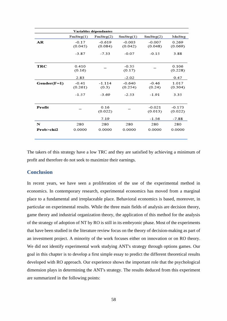
58
The takers of this strategy have a low TRC and they are satisfied by achieving a minimum of
profit and therefore do not seek to maximize their earnings.
Conclusion
In recent years, we have seen a proliferation of the use of the experimental method in
economics. In contemporary research, experimental economics has moved from a marginal
place to a fundamental and irreplaceable place. Behavioral economics is based, moreover, in
particular on experimental results. While the three main fields of analysis are decision theory,
game theory and industrial organization theory, the application of this method for the analysis
of the strategy of adoption of NT by RO is still in its embryonic phase. Most of the experiments
that have been studied in the literature review focus on the theory of decision-making as part of
an investment project. A minority of the work focuses either on innovation or on RO theory.
We did not identify experimental work studying ANT's strategy through options games. Our
goal in this chapter is to develop a first simple essay to predict the different theoretical results
developed with RO approach. Our experience shows the important role that the psychological
dimension plays in determining the ANT's strategy. The results deduced from this experiment
are summarized in the following points:

59
1. Individuals are showers to losses, between 67.5% and 80% of choices focus on certain
decisions. However, the use of uncertain decisions was not negligible. In the absence of
the waiting option, a large number of projects favor the adoption of projects with
immediate high values. In this case, decision makers do not intuitively recognize the
value of waiting for the same project and generally opt for compulsive strategy.
2. The RO approach reinforces the leap-frog strategy and therefore increases the gain.
This confirms the theoretical result of the GW model, according to which the probability
of choosing the leap-frog strategy increases with the increase in the speed of arrival of
NT. In addition, it shows that those who opt for the compulsive strategy are risk-averse.
Risk-seeking decision-makers tend to adopt the leap-frog strategy. This deduction is
consistent with the models of Chronopoulos and Lumbreras (2016) and Alexander and
Chen (2019).
3. In the context of options games, the waiting strategy representing the stable Nash
balance is not experimentally verified. The pre-emption game dominates from the fifth
period. This result confirms the theoretical inferences of HK (case 1). In particular, it
seems that the pre-emption strategy is the most played, especially for projects that are
less risky and by the most risk-averse.
4. The repetition of the PD, in the case of a single project, does not induce the game "Tit
for Tat". However, we note that the waiting strategy is more adopted when the project
is more risky and decision makers are less risky.
5. When the number of technology available increases the choice of waiting strategy can
reach more than 70% on average. The deviation from the waiting strategy does not
appear to be beneficial. The waiting strategy arises in the FM and SM games: each
company enjoyed a monopoly profit. Thus, these results verify the predictions of the
HK model (case 2).
6. The choice of the FM and SM strategy is applied when the difference of risk aversion
and TRC are significant.
7. With a higher number of the project, the waiting strategy is maintained. The game of
FM and SM does not turn into a war of attrition despite the rise of competitive threats.
This preliminary finding contradicts the HK model (case 3) and thus requires further
investigation.

60
8. Driven by the achievement of high gains, the FM strategy is adopted by risk-seeking
who have a good ability to think cognitively. On the other hand, those who pursue a
threat strategy are risk-averse with low CRTs and low gains. SM has a low CRT.
These preliminary results work towards a new research axis incorporating the psychological
dimension when evaluating the adoption of NT by the RO approach. An extension of the ID3
algorithm, already developed as part of decision theory, to the framework of option game theory
can be a powerful tool for predicting ANT's proper strategy.