Master’s thesis · 30 hec · Advanced level Agricultural Economics and Management – Master’s Programme Degree thesis No 819 · ISSN 1401-4084 Uppsala 2013

iiii

The Swedish Demand for Food -A Conditional Rotterdam Model Approach

Tobias Häggmark Svensson

iiii

The Swedish Demand for Food – A Conditional Rotterdam Model Approach Tobias Häggmark Svensson Supervisor: Yves Surry, Swedish University of Agricultural Sciences, Department of Economics Examiner: Ing-Marie Gren, Swedish University of Agricultural Sciences, Department of Economics

Credits: 30 hec Level: A2E Course title: Degree Project in Economics Course code: EX0537 Programme/Education: Agricultural Economics and Management - Master’s Programme Faculty: Faculty of Natural Resources and Agricultural Sciences Place of publication: Uppsala Year of publication: 2013 Name of Series: Degree project/SLU, Department of Economics No: 819 ISSN 1401-4084

Online publication: http://stud.epsilon.slu.se

Key words: Conditional, Demand, Food, Rotterdam,Swedish, System

iii

Abstract

The demand for food is susceptible to variation in several factors. Knowledge about the

nature of food commodities and how consumers react are important for decision makers. The

Swedish consumers have decreased the budget share spent on food commodities during the

end of the 20th century (Eidstedt et al. 2009). The purpose of the study is therefore to analyze

the Swedish demand for food over the period 1980-2011. By estimating price and

expenditure elasticities for the Swedish consumers the nature of the demand can be found,

allowing for analysis of how consumers react to changes in price and expenditure. A

conditional Rotterdam demand system approach is used in order to find the elasticities.

Testing of separable utility structures is also conducted in order to verify plausible structures

for the Swedish consumers, which can be employed when constructing complete demand

systems.

The estimated result was obtained maintaining the hypothesis of the laws of demand. Given

the conditional approach, approximations of unconditional elasticities were computed. Both

the unconditional and conditional own-price elasticities indicate that the Swedish demand is

insensitive to price changes. The estimated conditional expenditure elasticities indicate a

mixed result between luxury commodities and necessities (sensitive and insensitive

commodities). The approximation of the unconditional expenditure elasticities does however

indicate that the demand is insensitive to expenditure changes. The robustness of the

expenditure elasticities is however uncertain given the problems of the Rotterdam approach,

a more flexible functional form for the expenditure elasticities is desired.

For the separable utility structures, the hypothesizes that; meat can be weakly separable

from other commodities, and the hypothesis that the demand can be weakly separable

according to; animal, vegetable-based and beverage products, could not be rejected. This

indicates that the verified structures can be incorporated in a complete demand system

reducing the risk of misspecification.

iv

v

Table of Content

i. List of Figures and Tables ............................................................................................................. vii

ii. Abbreviations ............................................................................................................................... viii

1. Introduction ..................................................................................................................................... 1

1.1 Problem Formulation and Purpose ................................................................................................ 2

1.2 Delimitations ................................................................................................................................. 4

1.3 Structure of the Thesis ............................................................................................................. 5

2. Literature Review and Background ................................................................................................. 6

2.1 The Rotterdam and the AIDS Approaches ................................................................................ 6

2.2 Separability ................................................................................................................................ 9

2.3 Previous Studies ...................................................................................................................... 11

2.4 Recent Changes in Non-Economic Factors ............................................................................. 15

2.5 Concluding Remarks ................................................................................................................... 17

3. Theoretical Framework ................................................................................................................. 19

3.1 Utility Maximisation ................................................................................................................... 19

3.2 The Expenditure Function ........................................................................................................... 20

3.2.1 Price and Income Elasticities ................................................................................................ 21

3.3 Laws of Demand ......................................................................................................................... 23

3.4 Separability in demand ................................................................................................................ 24

4. Empirical Framework ........................................................................................................................ 26

4.1 Separability in the Rotterdam Model .......................................................................................... 28

4.2 Model Testing and Specifications ............................................................................................... 29

5. Data ............................................................................................................................................... 32

5.1 Collection and Modification of Data ........................................................................................... 32

5.2 Analysis of Data .......................................................................................................................... 33

6. Results and Discussion .................................................................................................................. 37

6.1 Residual Diagnostics ................................................................................................................... 37

6.2 Model Specification Testing........................................................................................................ 39

6.3 Economic Results ........................................................................................................................ 42

6.3.1 Elasticities ................................................................................................................................ 42

6.3.1 Utility Structures .................................................................................................................. 43

6.4 Discussion ................................................................................................................................... 44

7. Conclusion ..................................................................................................................................... 52

8. References ..................................................................................................................................... 54

9. Appendices .................................................................................................................................... 56

vi

Appendix A ........................................................................................................................................... 56

Appendix B ........................................................................................................................................... 58

Appendix C ........................................................................................................................................... 63

Appendix D ........................................................................................................................................... 64

Appendix E ............................................................................................................................................ 65

Appendix F ............................................................................................................................................ 68

vii

i. List of Figures and Tables

Figures Page

Figure 2.1 Utility Tree- Edgerton et al. (1996) 12

Figure 2.2 Utility Tree –Lööv and Widell (2009) 12

Tables

Table 2.1: Previous Estimates of Expenditure Elasticities 13

Table 2.2: Previous Estimates of Own-Price Elasticities 13

Table 2.3: Ad-Valorem Tax Levels 17

Table 4.1: Overview of Model Specifications 30

Table 6.1: Overview of Residual Test Results 37

Table 6.2: Values of Estimated Equations 38

Table 6.3: Log-Likelihood Values 39

Table 6.4: Testing for the Inclusion of the Intercept 40

Table 6.5: Tests of Laws of Demand 41

Table 6.6: Estimated Conditional Expenditure Elasticities 42

Table 6.7: Estimated Conditional Own-price Elasticities 43

Table 6.8: Testing of Separability Structures 44

Table 6.9: Unconditional Marshallian Elasticities 47

Table 6.10: Unconditional Expenditure Elasticities 48

viii

ii. Abbreviations

AC: Alston and Chalfant

AIDS: Almost Ideal Demand System

COICOP: Classification of Individual Consumption According to Purpose

DW: Durbin-Watson

FAO: Food and Agricultural Organization of the United Nations

JB: Jarque-Bera

LM: Lagrange Multiplier

LA-AIDS: Linearly Approximated Almost Ideal Demand System

LR: Likelihood-ratio

LSQ: Least Squares

NFA: National Food Agency

OLS: Ordinary Least Squares

SBA: Swedish Board of Agriculture

SNR: Swedish Nutrition Recommendations

SSR: Sum of Squared Residuals

SUR: Seemingly Unrelated Regression

USDA: U.S Department of Agriculture

1

1. Introduction

Studying the demand for food is an important topic. The demand is susceptible to variations in several

variables such as, trends, price, official nutrition recommendations, income (Eidstedt et al. 2009). In

recent times the per capita expenditure on food in Sweden has experienced a slight increase after the

decrease in the 1990’s, see figure 5.4 in appendix B. Foodstuff has however decreased its budget share

of total private consumption to around 10-15 % in the mid-2000’s (Eidstedt et al. 2009). Changes in

price are undeniably an important factor for the quantity demanded and during the 1980’s and 1990’s

the price development for food in Sweden was above the general price level indicating that food

became relatively more expensive, however this relationship changes after the mid-1990’s (Lööv and

Widell 2009).

Usually food is viewed as a necessity at the aggregate level. In some instances however, some food

items have been found to be classified as superior or luxury goods. Through demand system analysis

and with the help of elasticity estimates it is possible to analyze the nature of demand and make such

classification of commodities, and it also allows for studying of the interactive effects between goods.

Estimation of elasticities is also fundamental for policy work, and for conducting welfare analysis, e.g.

providing relevant information on the effects of raising or lowering taxes. With the recent focus of

environmental friendly consumption and production policies, switching behavior to environmental

friendly activities are attractive, which in the end affects the consumers. Taxation of certain

environmental damaging goods has been considered, e.g. one recent suggestion was taxation of meat

(Olsson 2013). By using appropriate elasticities and welfare analysis it is possible to analyze the costs

and benefits of implementing such a policy.

Further, a common problem for a consumer both in economic theory and in everyday life is to

efficiently allocate a budget. It is not hard to imagine that one makes his or her own household budget

for a broad group of categories such as, foodstuff, food away-from-home, and non-foodstuff. The non-

food category can include several sub-groups of durable goods and services, i.e. traveling and cars etc.

The budgeting problem is something almost everyone can relate to, hence it is a part of consumer

theory. In economic theory and modeling this concept is referred to as multistage-budgeting and

separability. Introducing the notion of separability then requires some a priori assumptions regarding

which consumption decisions that can be viewed as separable from each other (Edgerton 1997). These

assumptions can then have impact on the result of the study and thus needs to be evaluated. It has been

argued that specification issues are usually overlooked when conducting applied research and deserves

more focus (Edgerton 1997). If for example, a wrong separable structure is assumed and imposed it

can have implications on the estimated elasticities, and in the worst case might result in bad policy

decisions. As discussed in Edgerton (1997), the notion separability is common in studies regarding

2

food demand, and especially when estimating the demand for meat or alcoholic beverages where the

demand is supposed to be separable from demand of other food commodities. Albeit this is a plausible

assumption, it must be taken under consideration. For instance, it is possible that the consumer is not

explicitly interested in the meat product but might consider different sources of protein. Protein can be

found in a wide range of food commodities from vegetables to meat. Is it then plausible to separate

meat from other groups, or is a separable structure which is focused on the nutritional value more

appropriate? It might also be the case that some structures regarding the demand for food are true for

markets in certain countries but might not be applicable in regions with other consumption behavior

and patterns. It is thus of interest to research appropriate separable structure for the Swedish food

demand.

When studying consumer demand and the decisions made by consumers, appropriate modeling of the

behavior based on consumer theory, and the laws of demand is essential. It is also necessary to have an

appropriate way to reduce the amount of commodities which have to be considered when modeling

consumer demand. Demand system models have been designed with the purpose to be an

approximation of the consumer consumption decisions. The Almost Ideal Demand System (AIDS), the

trans-log model and the Rotterdam model are all demand systems with different specifications and

functional forms with foundation in consumption theory (Barnett 2007). However theory does not give

any advice on the best specification or model and leaves a lot of question on how to specify a model

(Edgerton 1997). Furthermore, since demand system analysis is a widespread topic, common across

many studies is to ignore specification issues and the effects of a priori assumptions and focus on the

economic result of the estimation process and not the applicability of the assumptions made in the

estimation procedure (Edgerton 1997). Thus in this study significant time is spent on the nature of the

conditions imposed in the estimation procedure in order to be able to make a sound analysis based on

consistent results.

Models as referred to above have been developed over several decades. The one used in this study, the

Rotterdam approach, was presented by Theil in 1980, and has been further developed during the

course of time. Demand system models have been considered to be particular suitable to analyze

consumer demand thus implying that the results can be viewed to be consistent with economic theory

(Alston and Chalfant (AC) (1993). Therefore this study will examine the Swedish demand for food

over the period 1980-2011 by estimating a conditional Rotterdam demand system.

1.1 Problem Formulation and Purpose

Food expenditure has a relatively significant expenditure share and therefore studies regarding the

domestic demand for food are an important topic. In 1992 the expenditure on food accounted for 20 %

of a household’s total expenditure. In the mid-2000’s total expenditure share on food had decreased to

around 10-15 % (Eidstedt et al. 2009). Changes in prices can affect the welfare of consumer, therefore

3

knowledge regarding consumer reactions to changes in variables affecting the demand for certain

commodities is important to study. This topic has been studied before but in order to make sound

decisions one needs recent information. For policy decisions, institutions have to conduct welfare

analysis and in order to reach correct conclusions, elasticity estimates done on an appropriate basis is

needed, as well as a complete understanding of the reason behind the result.

In order to arrive at good elasticity estimates one has to make sure the result follows economic theory.

If the estimates do not follow theory and this is not acknowledged, decisions made might lead to

effects which are not desired. However, when conducting applied econometrics there is always a

trade-off between specifying a model which is consistent with economic theory or is correctly

specified in terms of statistics. Parameter estimates which do not follow economic theory is of lower

value, on the other hand the same is true for statistic modeling with spurious results. Hence one must

make sure the economic theory is imposed without reducing the statistical performance to a larger

extent. Therefore a significant time in this study is spent on making sure that the parameter estimates

follow desired economic theory, such as the laws of demand.

Assuming separability provides a great deal of convenience in the estimation procedure allowing for

specific foodstuff commodities to be analyzed without paying attention to consumption of other goods

(Moschini et al. 1994). The concept is also, almost employed in every applied study, hence derivation

of correct structures is essential (Edgerton 1997). Assuming separability allows for estimation of

conditional demand system. However conditional elasticities lose information regarding changes in

allocation of expenditure and become less appropriate for policy analysis. It follows that the

imposition of separable structures in the utility functions has been proved to be true for certain demand

in some countries, it is thus of interest to apply and test different structures for the Swedish consumers.

If the tested structures are found to be relevant for the Swedish demand for food the result can be used

to justify more detailed studies of the Swedish demand for food and construct full demand systems.

The purpose of the study is to examine the Swedish demand for food over the period 1980-2011 and

analyze how sensitive the demand is to changes in price and expenditure by estimating a conditional

Rotterdam demand system. The aim is also to test and analyze separable utility structures. In order to

find the nature and properties of the Swedish demand the following will be conducted:

Estimation of conditional price and expenditure elasticities for a set of food commodities.

Testing of two separable utility structures by having:

1. Meat as a separable commodity.

2. Three major separable commodity groups (animal and vegetable-based and beverages

products).

4

1.2 Delimitations

The study will cover the period from 1980 to 2011. The choice of this sample time frame is based on

the availability of homogenous data. From 1980 there are price indices available according to the

international Classification of Individual Consumption According to Purpose (COICOP). When

conducting research on time series data one has to deal with the problem of non-homogenous datasets.

The source responsible for collecting the data can change how the primary data is collected. In order to

deal with the problem of non-homogenous datasets and still model a complete set of foodstuff

commodities which the consumer can choose from, the COICOP classification is used to make sure

that the groups included in the dataset is as homogenous as possible throughout the complete period.

The COICOP classification is the current method used by Statistics Sweden and similar institutions for

dividing commodities into higher aggregated groups. By using international classification standards

the comparison of results can easily be done. Hence the aggregation has been done in accordance to

the groups included in COICOP. The following ten aggregate commodity groups included in

COICOP are the ones of interest.

Bread and other cereal products

Meat

Fish,

Milk, cheese and eggs,

Oil and fat

Fruit and vegetables

Sweets and ice cream

Other foodstuff

Non-alcoholic beverages

Alcoholic Beverages

Including these ten commodities are done in order to try to estimate a complete set of commodities a

consumer can choose from. By including the whole range of food commodities which a consumer can

choose from the result will hopefully be close to the real consumption choices a consumer makes.

Unfortunately the commodity group fish is not estimated in the final result due to data unreliability,

which is more closely discussed in chapter 5. Non-economic factors affecting the demand for food are

somewhat difficult to capture completely by demand system analysis and therefore does not fit the

scope of the study completely, however chapter 2.3 discusses some relevant non-economic factors.

Testing for trends is also conducted which indicates if changes in non-economic factors are present.

The understanding of these factors can be essential for changes in expenditure.

5

1.3 Structure of the Thesis

The remaining sections of the thesis are organized as follows. In chapter two, literature on the demand

system approach and previous studies of the Swedish demand for food will be reviewed. In chapter

three and four the theoretical and empirical model will be explained. Chapter five will refer to the

dataset used for the study. And in the final chapters, chapter six and seven, the results will be

presented and discussed, and a conclusion will be given.

6

2. Literature Review and Background

The purpose of this section is to discuss previous studies relevant to the research done in this paper.

Earlier studies in the field of demand system analysis can be divided into two categories. The first

category is research focused on purely econometric issues of demand system analysis, i.e. relevant

assumptions and performance of demand systems. The other category refers to applying the demand

system approach in order to obtain estimates of price and income elasticities. Hence this chapter will

be divided accordingly, where one section refers to the performance of the demand system approach

and specifically the Rotterdam model and the AIDS model. Incorporating the AIDS model is due to

the fact that it has widespread use and is used in the most recent Swedish studies. It is necessary for

the understanding of why the Rotterdam approach has been chosen for this study. The Rotterdam

approach is explained in chapter four and the AIDS approach is briefly explained in appendix A. The

second section of this chapter will refer to application of demand systems and relevant studies of the

Swedish demand for food discussing both non-economic and economic variables.

One apparent problem which any model faces is the data used when applying the demand system

approach (Barten 1977). As mentioned, the demand system method is derived from individual

consumer’s behaviour, but data for specific consumers seldom exists and thus forces the researcher to

use highly aggregated commodities data. By using aggregate data in order to find per capita

consumption one is forced to divide with the population size. This implies that all consumers face an

identical demand function, and thus respond equally to changes in price or income (Barten 1977). The

question is then; is it plausible to replace each individuals demand function with an average demand

function? The assumption of a representative consumer is questionable, but due to the available data

material it is sometimes not possible to work around this problem. However, according to Barten

(1977) the matter of exact aggregation is of less importance compared to the one of consistent

aggregation. By examining the covariance matrixes, which should tend to zero, the nature of

consistent aggregation can be evaluated (Barten 1977). Information regarding the average change can

also be useful for generalizations. The aggregation problem is less apparent in the Rotterdam

approach, where one does not have to specify an explicit utility function. Thus the representative

consumer’s utility function is not present and one does not have to make any specific assumptions

regarding the functional form of the utility function.

2.1 The Rotterdam and the AIDS Approaches

The performance and the specification of the approach used in applied work are of great importance,

since occasionally results can be attributed to the specification of the model used. In demand system

analysis the model specification refers to the functional form for the consumer that is used but also

7

assumptions regarding the behaviour of consumers’ consumption decisions. The behaviour of

consumers originates microeconomics and consumer theory. Hence the theory in which the Rotterdam

model and the AIDS model are derived from is the same.

One obvious similarity is that both the Rotterdam and the AIDS approaches have the same

requirements for data, thus removing one factor which can cause the result to be different, as well as

the econometric behaviour cannot be attributed to the data needed in the estimation procedure. In

Dameus et al. (2002) comparison between the two models is conducted by using both approaches on

U.S meat demand data. By estimating both models with the same dataset and setting one model as the

null hypothesis Dameus et al. (2002) found that the AIDS approach was rejected in favour of the

Rotterdam approach. This is of interest since the recent applied work by Lööv and Widell (2009) uses

an AIDS approach for both a complete set of food commodities and an explicit analysis for the

demand for meat in Sweden. More specifically the study by the Lööv and Widell uses a linear

approximation of the AIDS model (LA-AIDS) in the estimation procedures for all goods, and in the

analysis of the meat demand. Hence the basis of why Lööv and Widell (2009) chose the LA-AIDS

approach can be questioned, and the Rotterdam approach might have been better suited for the study

of meat demand. The AIDS approach experienced popularity because it is relatively easy to estimate

and interpret and therefore the Rotterdam approach does not receive the attention it deserves (AC

1993). Even though the LA-AIDS model has been used in a lot of studies, arbitrarily picking a model

based on the common usage without emphasizing on the applicability can have impact on the results.

Therefore it is necessary to point out that there are several studies available that discuss problems with

the LA-AIDS model.

According to Barnett (2007), the linear approximation of the AIDS model might not produce

consistent results compared to the true model it is supposed to approximate, i.e. the full non-linear

model. When comparing estimates between a full non-linear AIDS model (PIGLOG), which the LA-

AIDS is supposed to approximate and the LA-AIDS estimates, Barnett (2007) by Monte-Carlo

simulations found that they do not produce the same elasticity estimates. The full non-linear AIDS

model has a problem with the signs of the elasticities, and according to Barnett (2007) this problem

becomes worse when linearly approximating the model. This implies that it is possible for the LA-

AIDS model to produce estimates that classifies goods as complements when they in fact should be

substitutes. This must be considered when interpreting the result of estimates from such a model.

AC (1993) argues that, even though the Rotterdam and the AIDS approach have several similar

features and identical data requirements and can thus be viewed as equally attractive, they can often

lead to different results when applying them. In AC’s study they constructed a test for evaluating the

applicability of the Rotterdam system or the LA-AIDS. Applying this to meat demand data showed

that the LA-AIDS model could be rejected in favour for the Rotterdam model. However the authors

8

point out that this is not evidence that the Rotterdam model is generally stronger than the LA-AIDS

model, merely only that one needs test the applicability when choosing the model type when

conducting a study. This is however another study that rejects the AIDS approach, to some extent, in

favour of the Rotterdam model when specifically dealing with meat demand and thus can be viewed to

emphasize the need for a Rotterdam demand system to be estimated for the Swedish food demand and

see if the results differ. One could therefore argue that the specific analysis of the Swedish meat

demand conducted by Lööv and Widell (2009) should have been carried out with a Rotterdam

approach instead.

LaFrance however claims that the points made by AC are erroneous. LaFrance (1998) argues that the

statistical method used for testing the LA-AIDS model versus the Rotterdam demand system inflates

the test statistic. The ordinary least square (OLS) regression by AC has a non-linear transformation of

the dependent variable as regressors, resulting in multicollinearity among the independent variables.

LaFrance continues with constructing a maximum-likelihood test and finds that no model can be

rejected in favour of the other. Conversely, Dameus et al. (2002), claims that LaFrance conclusion

could be attributed to the low power of the test used in evaluating the models. The general conclusion

in Dameus et al. (2002) is that it is always necessary to assess the models econometrically. This is

unarguably the most reasonable conclusion.

Weaknesses of the Rotterdam approach have been pointed out by Clements et al. (1996). The

specification and parameterization of the Rotterdam model causes the marginal budget shares to be

constant over time. It follows that increased wealth causes the income elasticities of necessities to rise

while luxuries will fall (Clements et al. 1996). The following effect is that food becomes less of a

necessity and more of a luxury good when wealth increases. According to Clements et al. (1996) this

is not plausible, as individuals become better off food should become less of a luxury good and due to

the constant shares it has been argued that the Rotterdam model is only consistent with Cobb-Douglas

utility functions. In favor of the constant share it is argued that when dealing with time series data

changes in expenditure shares are moderate (Clements et al. 1996). It is important to note the

economic implication of the Rotterdam parameterization will result in linear Engel curves Neves

(1994). This implies that as income increases the quantity demanded will always increase with the

same proportion. Usually Engel curves imply that the increase in quantity demanded for certain food

commodities will fall off as expenditure increases and demand get saturated.

From the previous review it follows that when dealing with statistical and econometrical evaluation of

models, the conclusion often depends on the nature of the statistical test, and its specification.

Therefore for the purpose of discussion it is necessary to point out that conclusions derived from one

test can be proven wrong by another approach, which is supposed to be better specified. This will, to

9

some extent, be considered in this study, where two test statistics will be presented for the likelihood-

ratio values and allows for an opinion regarding the effects of the test statistic used.

2.2 Separability

The notion of separability is a common assumption for demand system analysis and is usually

assumed in all applications (Moschini et al. 1994). Due to the implication of assuming or imposing

separability it is essential to discuss the properties behind. Separability can be defined as weakly

separable. Briefly, weak separability of consumer demand can be explained as follows; the marginal

rate of substitution for two commodities in the same group is not affected by the consumption of a

commodity in a different group (Edgerton et al. 1996). A more detailed explanation can be found in

chapter three. As discussed by Edgerton (1997) assuming separability is of course plausible, but

incorrectly assumed separable structures will lead to wrong conclusions and decisions. It is also an

assumption that in some cases can be easy to imagine being plausible, i.e. consumption decisions

regarding durables and foodstuff. Separability thus requires some a priori knowledge on how to divide

commodities into groups (Edgerton et al. 1996). If a researcher is interested in applying the demand

system approach and does not assume weak separability there are three choices.

The first choice is to estimate a complete demand system with extremely high aggregated commodity

groups such as food, clothing and housing etc. (LaFrance 1991). This approach however is attributed

with drawbacks. Highly aggregated price and commodity groups require restrictive conditions in order

to be consistent with consumer preferences. It also follows that a great deal of information regarding

demand for specific goods is lost and more detailed conclusions are hard to make if lower stages are

not included (LaFrance 1991).

A second alternative is to specify an incomplete system of demand equations dependent on the prices

of the relevant good, related goods and expenditure (LaFrance 1991). Specifying incomplete demand

systems implies that the information regarding the upper stage of the budgeting process is minor, i.e.

higher aggregated commodities are not are not included in the system, and income is replaced with

expenditure and thus assuming that the commodity group of interest is weakly separable from the

other commodity groups. It follows that this will yield conditional demand equations. This approach

has been argued to be ad hoc and is sometimes not consistent with the theory which the demand

system approach originates from (LaFrance 1991). For this study, this approach is used, implying that

the demand for food is assumed to be weakly separable from the demand of other non-food

commodities and thus using expenditure on foodstuff instead of disposable income. Due to the

arguments by LaFrance it is important to make sure that the model follows the conditions set out by

economic theory, i.e. the laws of demand, by enforcing them on the estimated parameters. It is also

important to fully understand the implications of a conditional system.

10

Separability can be imposed on a full demand system and is thus the third choice available (Moschini

et al. 1994). In this case it implies that if one is interested in a certain commodity group it is necessary

to specify at least one upper budget level, including the group of interest and a group representing all

other commodities, e.g. one commodity group for non-food and one commodity group for foodstuff

which then contain information on several commodities. Imposing separability implies that the

commodity group of interest has a demand function dependant on the prices of each respective

commodity included in the group and the total expenditure of that group and the total expenditure of

the second group. The two groups included are still affected by price changes in the other group

indirectly, through the allocation of expenditure. By specifying this type of demand system more

information regarding the upper level can be obtained, and the elasticities are better suited for policy

analysis since at the last stage they will be unconditional.

The use of conditional demand equations is therefore attributed with some drawbacks. When assuming

separability it is usually the bottom level that is of interest since it is more detailed. It is therefore the

case that the allocation of income in the upper level is left unspecified for conditional systems and by

doing so the elasticity estimates loses the information regarding changes in the upper level i.e. changes

in allocation of expenditure between commodity groups (Moschini et al. 1994). In Moschini and Moro

(1993) a complete demand system is estimated, it follows that the greatest differences between

conditional and unconditional elasticities occur for expenditure, where the unconditional expenditure

is significantly lower. The difference for the Hicksian and Marshallian elasticities are minor, the

Hicksian is supposed to be large in absolute value while the opposite is true for the Marshallian.

Edgerton (1997) compares conditional and unconditional elasticities according to the utility tree

described in figure 2.1 using OLS and seemingly unrelated regression (SUR). Testing the null-

hypothesis that all the unconditional elasticities are equal to the conditional in the system, Edgerton

(1997) concludes that there are differences in the unconditional and conditional elasticities. However

the necessary and sufficient conditions for conditional demand equations will however exist if the

direct utility function can be assumed to be weakly separated (Moschini et al. 1994). Moschini et al.

(1994) test if the notion of separability is viable for applied work, and tests three types of weakly

separable structures imposed on a Rotterdam demand model using U.S data. The three separable

structures refer to, separating non-food and foodstuff, the second structure being the separation of

meat, to other food commodities, within the foodstuff category. The third structure refers to keeping

non-food and foodstuff separated and dividing the groups included in foodstuff category between meat

and nonmeat. The result of their study is that the widespread use of separability is justified. Hence it is

assumed in this study that the demand for food is weakly separated from demand of non-food allowing

for a conditional demand system. However the points made by Edgerton (1997) regarding the

difference between conditional and unconditional elasticities are still evident and imply that the

conditional result of this study is not suitable for policy evaluation.

11

It follows that specifying conditional demand systems can cause econometric problems due to the fact

that now expenditure on commodities can be endogenous. Moschini et al. (1994) suggests one way of

dealing with these two problems. The problem of endogeneity can be solved by imposing separability

on a complete demand system that includes all available goods. This demand system would not have

the problem of endogenous expenditure and the allocation of income in the first level of the utility tree

would occur according to theory. This procedure however requires a detailed data set for all the

relevant categories of goods and yields a lot of equations.

To diversify the discussion LaFrance (1991) however claims that expenditure in separable demand

systems is never exogenous even for full demand systems, unfortunately implying that the problem of

endogenous expenditure is always present since total expenditure is the sum of the expenditure on all

commodities. LaFrance’s conclusion however is that even though the problem of endogeneity is

present, there is simply not a better alternative than the approach of assuming separable demand

systems and thus conditional demand functions. The correct method is therefore to acknowledge the

limitations and choose correct variables for the conditional demand functions and to pay respect to the

distribution of the residuals, overlooking to do so can have serious impact on applied work (LaFrance

1991).

2.3 Previous Studies

Econometric evaluation is necessary in order to make appropriate applied work, and allows for an

applied economist to choose correct specifications. Since this study’s main goal however is to estimate

a Rotterdam demand system for Sweden it is essential to discuss recent studies in the applied field that

refers to the Swedish demand for food.

Edgerton et al. (1996), as mentioned, have conducted a demand system analysis of Sweden and the

other Nordic countries. U.S Department of Agriculture (USDA) (2003) estimated a full demand

system with several budget stages for several countries, including Sweden. Lööv and Widell (2009)

constructed a conditional demand system for the Swedish demand which is the most recent study, and

therefore does not provide unconditional elasticities.

The AIDS model is used in Edgerton et al. (1996) and Lööv and Widell (2009), both estimate

elasticities for food commodities. In order to understand the estimation procedures the utility trees

assumed in the studies by Edgerton et al. (1996) and Lööv and Widell (2009) are shown in figure 2.1

and 2.2 respectively.

12

Private Consumption

Food-at-Home

Animalia

Meat

Fish

Milk, Egg

and Cheese

Beverages

SoftDrinks

Hot Drinks

Alcoholic Drinks

Vegetabilia

Bread and Cereals

Friut and Vegetables

Potatoes

Miscellaneous

Fats and Oils

Sugar

Confectionery

Restaurants and Cafés

Non-Durables Services

Private Consumption

Food-at-home

Bread and Cereal Products

Meat and Meat Products

Fish Milk, Cream,

Cheese and Eggs Fruit and Berries Vegetables

Potato and Potato Products

Non-Food

By looking at figure 2.1 it is evident that the study by Edgerton et al. (1996) is a three stage budgeting

process including other non-durables, restaurants, cafés and other services in the first stage, while

Lööv and Widell (2009), (figure 2.2), have focused explicitly on the Swedish demand for food. Hence

Lööv and Widell estimate a conditional demand system, assuming that food-at-home is weakly

separable from non-food. In their study, the non-food category is not included in the estimation

procedure. For Edgerton et al. (1996) the utility tree implies a full demand system, according to the

upper level, where only consumption of durables has been left out. The decision not to include durable

goods in the study is based on the problems regarding consumption of durable goods due to the nature

of time periods. The definition used for private consumption is however widespread (Edgerton et al.

1996). The utility tree as depicted in figure 2.2 has close resemblance to the utility tree that will be

assumed for the estimation procedure in this study.

Figure 2.1 Utility Tree- Edgerton et al. (1996), p. 7

Figure 2.2 Utility Tree –Lööv and Widell (2009)

13

Previous Estimates

Table 2.2. Previous Estimates of Own-Price Elasticities

Product Group Conditional, Marshallian Unconditional, Marshallian

1980-2006 1963-1989 1963-1989

Lööv and Widell Edgerton et al. Edgerton et al.

Bread and Cereal Products -0.77 -1.00 -0.71

Meat and Meat Products -1.12 -0.61 -0.35

Fish -0.35 -0.28 -0.26

Milk, Cream, Cheese and Eggs -0.47 -0.14 0.00

Fruits and Berries -0.39 - -

Vegetables -0.58 -0.71 -0.57

Potato and Potato Products -0.18 0.15 0.14

Alcoholic Drinks - -0.96 -0.85

Confectionery etc - -0.73 -0.43

Oil and Fats - -0.52 -0.34

Non-Alcoholic Beverages - -0.33 -0.32

Table 2.1 Previous Estimates of Income (expenditure) Elasticities

Product Group Conditional Unconditional

Lööv and Widell Edgerton et al. Edgerton et al.

Bread and Cereal Products 1.39 1.39 0.61

Meat and Meat Products 1.29 1.24 0.64

Fish 1.78 0.35 0.18

Milk, Cream, Cheese and Eggs 0.20 0.92 0.47

Fruits and Berries 0.79 - -

Vegetables 0.99 0.78 0.34

Potato and Potato Products -0.30 -0.22 -0.10

Alcoholic Drinks - 1.21 0.62

Confectionery etc - 1.00 0.37

Oil and Fats - 1.43 0.53

Non-Alcoholic Beverages - 0.51 0.26

14

Table 2.1 shows the expenditure elasticities for the two different studies while table 2.2 presents the

own-price elasticities. Some categories are not identical in the studies. The cross-price elasticities are

not shown here due to the great number of them. In Edgerton et al. (1996) both unconditional and

conditional elasticities are available due to the specification of the utility tree, while the elasticities

from Lööv and Widell only refer to the conditional ones. The conditional elasticities are thus

comparable. The difference between the unconditional and the conditional elasticities in Edgerton et

al. is because the elasticities of the upper stages affect the elasticity of meat, e.g. elasticity for animalia

and food-at-home affects the elasticity for meat. Multiplying the expenditure elasticity for animalia

and food-at-home with the expenditure elasticity for meat will give the unconditional expenditure

elasticity of meat. It is expected the unconditional expenditure elasticity has a lower value than the

conditional. The unconditional elasticities should be in line with the Engle Law stating that income

elasticity for food commodities should not be greater than 1. For the unconditional price elasticities

several effects are included. The direct effect will be the conditional elasticity, and the indirect effect

will refer to how the allocation of expenditure changes due to a price change (Edgerton et al. 1996).

The studies also classify commodities as necessities, luxury and inferior goods. Classification between

these categories is done by analysing the conditional expenditure elasticities and the unconditional

from Edgerton et al. (1996). Following the utility tree given for Edgerton et al. (1996) the food-at-

home category was found to be a necessity. The other categories, restaurants and non-durables were

found to be luxury goods. And since these categories are not included in the study by Lööv and

Widell, the results are not possible to compare. The third stage is however comparable. Edgerton et al.

(1996) found that fish, non-alcoholic beverages, fruit and vegetables and milk, cheese, cream and eggs

were to be necessities while bread and cereals, meat, alcoholic drinks, confectionary, and fat and oils

were found to be luxury commodities, examining the conditional elasticities. The two groups, sugar

and potato were classified by Edgerton et al. (1996) to be inferior goods. Lööv and Widell (2009)

classified the goods in the following manner; bread and cereal, meat and fish were found to be luxury

goods, while fruit and berries, vegetables, milk, cream, egg and cheese were necessities and classified

potato as an inferior commodity. The studies thus found different results regarding the classification of

fish. It is possible that the different classification is a result from the different time periods covered.

The consumption of fresh fish has been decreasing constantly during the 20th century and fish

consumption becomes more of the luxurious kind (Lööv and Widell 2009). It is interesting to note that

both studies classify potato as an inferior good and thus it might be plausible to classify potato as such,

even though it is an unusual economic phenomenon. The estimated cross-price elasticities in Lööv and

Widell’s study indicates that there are gross substitution and complementary effects present, although

they are moderate.

The studies also classify the commodities as being either elastic by using own-price elasticities,

inelastic or Giffen goods. The result presented in Edgerton et al. (1996) shows no commodity is to be

15

considered as price elastic using the conditional elasticities, instead the majority of commodities are

considered as inelastic while bread and cereal products are on the limit. The commodities that were not

found to be inelastic were instead classified as Giffen goods. This is however claimed by Edgerton et

al. (1996) to be a rather rare economic occurrence, and it is more likely that it is a case of

misspecification, and the conclusion is that the commodities that are classified as Giffen goods should

be viewed carefully. Lööv and Widell (2009) found that, with the exception of meat which is classified

as elastic, all other commodities in the study are inelastic. It thus follows that the studies found that the

Swedish demand for food, using the AIDS approach, is somewhat insensitive to changes in price, due

to the classification of inelastic demand.

Both studies estimate the Swedish demand for food use the AIDS approach. Lööv and Widell (2009)

specifically use the LA-AIDS, implying that it is linearly approximated. As mentioned previously the

linear approximation of the AIDS approach is problematic. One problem refers to the sign of the

cross-price elasticity estimates, implying that it is a possibility to make wrong classification of goods

as complements. Lööv and Widell claim that no substitutes where found except that meat was a

substitute for fish, but not vice versa. They further argue that this is also theoretically consistent since

the commodity groups for the study implies that there should not be any substitutes. This is undeniably

a plausible statement, one would not expect milk and bread to be substitutes. But one could suspect

that other categories i.e. potato and cereal products, then referring to rice and pasta, to possibly be

substitutes. With the problems of the LA-AIDS model in mind, the statement by the Lööv and Widell

can consequently be questioned. The same reasoning is also true for the study conducted by Edgerton

et al. where the result compared to Lööv and Widell is mixed between complementary and substitute

commodities and to some extent might be more plausible. If the results are consistent with theory, one

could view them as a confident result, but if it is hard to theoretically classify the commodities, the

results could be considered as unreliable.

2.4 Recent Changes in Non-Economic Factors

Changes in non-economic variables can in some cases have a strong impact on the decisions made by

consumers. Variables viewed as non-economic can be; consumption habits, tastes, advertisement and

the population structure. Including this section is done in order to acknowledge effects which cannot

be fully captured by demand system analysis. It is however possible to some extent capture the non-

economic factors by introducing a trend variable in the demand system. In the study Consumption of

Food, 1960-2006, written by Eidstedt et al. (2009), the non-economic factors influencing consumer

demand are discussed.

Two major findings in the study carried out by Eidstedt et al. (2009) are that the consumption

behaviour has changed, favouring processed products such as industry baked bread and premade food

products. This implies that the total consumption of e.g. flour has been fairly constant during the

16

investigated period while the direct consumption, which refers to consumption done by consumers,

has decreased. The second major finding is that the share of income spent on food has decreased as

disposable income increased. It follows that the decreased budget share spent on food commodities

implies that food has become less of a luxury good. It is evident that non-economic factors have

changed during the period and therefore, it is of interest to include a trend variable in the estimated

model. Some of this variation is captured by the trend variable.

Eidstedt et al. (2009) defines the most important non-economic factors as:

Demographics

Attitude towards recommendations from the National Food Agency

Safe foodstuff

Lifestyle

Technological progress

Advertisement

These factors have the possibility to influence the consumption decisions. During the investigated

period the National Food Agency (NFA) has published several Swedish nutrition recommendations

(SNR), 1981, 1989, 1997 and 2005. During the period of interest the NFA has published four reports

that can have an effect on the consumption of food products. It is possible that these recommendations

has solidified the need for certain food products in order to construct a proper meal and can therefore

affect consumption patterns.

Important changes in our lifestyle that affects food consumption patterns are according to Eidstedt et

al. (2009); increased time spent working, increased disposable income and technological progress. The

increased time spent working and technological progress could be one of the reasons why food

consumption has shifted in favour of processed and ready-made food. The increase in the amount of

working hours refers to the amount of women that has entered the workforce. If both partners in a

relationship or a family are working, less time is available for cooking (Eidstedt et al. 2009). This can

further increase the demand for processed food and pre-made food products.

Increased knowledge regarding the food chain and exposure of misconduct in the process has impact

on the consumers’ decision (Eidstedt et al. 2009). Hence knowledge of additives in food and hygiene

in the food chain plays an important role for short term variations in the consumers’ choice of food.

Consumers will tend to buy safe foodstuff, meaning that the consumer is confident that the commodity

fulfils her requirements. Exposure of misconduct by the media is therefore of importance on

consumption habits.

17

An important factor for the development of price during the investigated period is the Swedish

agricultural policy. The agricultural market was regulated until 1990 meaning that the price level, and

especially producer prices, was not completely decided by market forces. The general price level was

instead decided by a group of important actors on the agricultural market, both consumer and producer

organisations and the government (Eidstedt et al. 2009). Removal of agricultural regulations also

included, adjustment of the ad valorem tax. These changes will be visible when graphically examining

the data set. The Swedish market was also harmonized in accordance with EU regulations, so the

Swedish agricultural market had the same rules as the EU market. It is evident that during the period

of interest, political decisions have influenced the producer price level on certain products and thus the

consumer price level, it is therefore plausible that consumers’ decisions have been affected. Important

changes in the ad-valorem tax during the period due to the agricultural policy which can have effect on

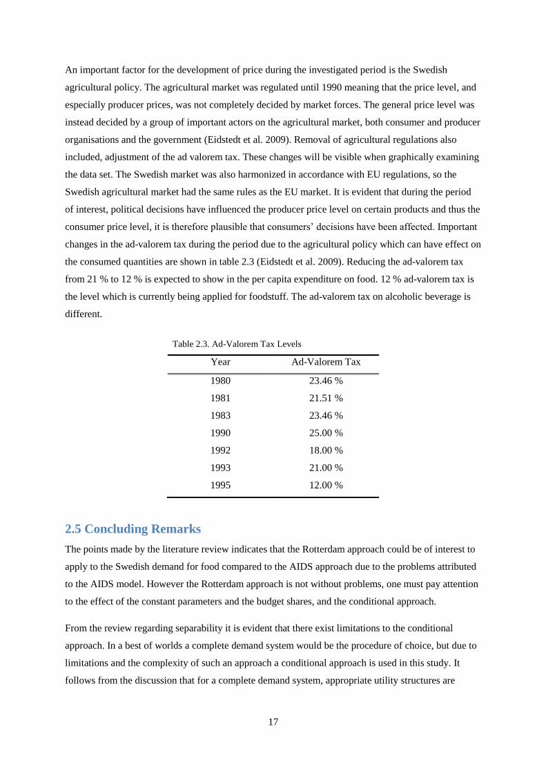
the consumed quantities are shown in table 2.3 (Eidstedt et al. 2009). Reducing the ad-valorem tax

from 21 % to 12 % is expected to show in the per capita expenditure on food. 12 % ad-valorem tax is

the level which is currently being applied for foodstuff. The ad-valorem tax on alcoholic beverage is

different.

2.5 Concluding Remarks

The points made by the literature review indicates that the Rotterdam approach could be of interest to

apply to the Swedish demand for food compared to the AIDS approach due to the problems attributed

to the AIDS model. However the Rotterdam approach is not without problems, one must pay attention

to the effect of the constant parameters and the budget shares, and the conditional approach.

From the review regarding separability it is evident that there exist limitations to the conditional

approach. In a best of worlds a complete demand system would be the procedure of choice, but due to

limitations and the complexity of such an approach a conditional approach is used in this study. It

follows from the discussion that for a complete demand system, appropriate utility structures are

Table 2.3. Ad-Valorem Tax Levels

Year Ad-Valorem Tax

1980 23.46 %

1981 21.51 %

1983 23.46 %

1990 25.00 %

1992 18.00 %

1993 21.00 %

1995 12.00 %

18

necessary. Depending on the result the tested structures can be used when constructing a complete or

full demand system for Sweden if they are found applicable to the Swedish data set.

The previous estimates will be discussed and compared to the result of this study. It follows from the

previous estimates that the Swedish demand for food is to be considered as relatively insensitive to

price changes regardless of a conditional or unconditional approach using the AIDS system. For the

expenditure sensitiveness it is evident that the result depends on the approach chosen.

19

3. Theoretical Framework

Consumer demand theory, based on microeconomics, will be the framework explaining consumer

behaviour. Therefore the purpose of this chapter is to explain the theory which is the foundation of the

empirical work conducted and which the results and the conclusion follow from. Mathematical

developments and demonstrations in this chapter are based on Edgerton et al. (1996) and Gravelle and

Rees (2004).

Worth noting before deriving the utility maximization problem is that the Rotterdam approach does

not use an explicitly formed utility function but is instead derived by total differentiation of a double

logarithmic demand function. It is also important to realize that the demand system estimated is a

conditional demand system, and the maximisation procedure will thus yield conditional demand

equations. However understanding of utility maximization is essential for consumer theory, and for

understanding of the demand equations. When specifying the utility tree it is also necessary to have

derived the utility function.

3.1 Utility Maximisation

The consumer maximizes utility according to a specific utility function and a budget constraint. By

allocating the available budget in the most efficient way, the consumer is able to maximize her own

utility. Theory assumes that the consumer is always trying to maximize utility and in order to achieve

a consistent utility function the consumer’s preference has the following properties (Edgerton et al.

1996) p. 55-56:

Let denote a consumption bundle.

I. Reflexive. Implies that if two commodities are equally good the consumer is indifferent.

II. Complete. The consumer is able to rank all the different consumption bundles e.g. the

consumer always has an opinion.

III. Transitive. Implies that the consumer’s preferences are consistent. I.e. and

then it follows that . Not fulfilling this assumption would cause the consumer to not be

able to select a best bundle.

IV. Continuous. The demand function is continuous, there is no specific quantity which is not

desired, the indifference curve has no breaks.

V. Strongly monotonic. The consumer always prefers more of a good than less of it. I.e. If is

larger than and then .

VI. Strictly convex. The consumer will always prefer a bundle that consists of a mix of

commodities. It can be explained by and yields the same utility as a

bundle where , then .

20

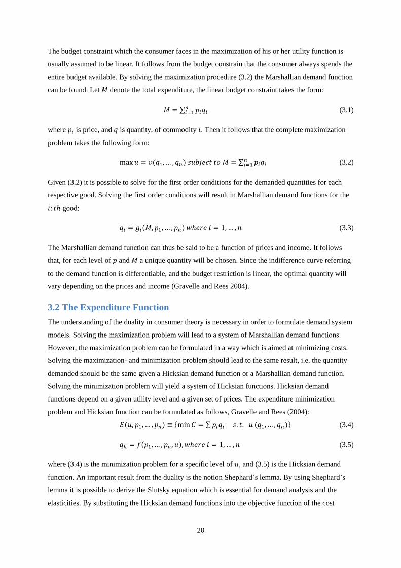
The budget constraint which the consumer faces in the maximization of his or her utility function is

usually assumed to be linear. It follows from the budget constrain that the consumer always spends the

entire budget available. By solving the maximization procedure (3.2) the Marshallian demand function

can be found. Let denote the total expenditure, the linear budget constraint takes the form:

∑ (3.1)

where is price, and is quantity, of commodity . Then it follows that the complete maximization

problem takes the following form:

∑ (3.2)

Given (3.2) it is possible to solve for the first order conditions for the demanded quantities for each

respective good. Solving the first order conditions will result in Marshallian demand functions for the

good:

(3.3)

The Marshallian demand function can thus be said to be a function of prices and income. It follows

that, for each level of and a unique quantity will be chosen. Since the indifference curve referring

to the demand function is differentiable, and the budget restriction is linear, the optimal quantity will

vary depending on the prices and income (Gravelle and Rees 2004).

3.2 The Expenditure Function

The understanding of the duality in consumer theory is necessary in order to formulate demand system

models. Solving the maximization problem will lead to a system of Marshallian demand functions.

However, the maximization problem can be formulated in a way which is aimed at minimizing costs.

Solving the maximization- and minimization problem should lead to the same result, i.e. the quantity

demanded should be the same given a Hicksian demand function or a Marshallian demand function.

Solving the minimization problem will yield a system of Hicksian functions. Hicksian demand

functions depend on a given utility level and a given set of prices. The expenditure minimization

problem and Hicksian function can be formulated as follows, Gravelle and Rees (2004):

{ ∑ } (3.4)

(3.5)

where (3.4) is the minimization problem for a specific level of , and (3.5) is the Hicksian demand

function. An important result from the duality is the notion Shephard’s lemma. By using Shephard’s

lemma it is possible to derive the Slutsky equation which is essential for demand analysis and the

elasticities. By substituting the Hicksian demand functions into the objective function of the cost

21

minimization problem one will find the expenditure function. The expenditure function shows the

lowest expenditure needed for a given utility level and a given set of prices. If the expenditure function

is available, then it is possible, through the use of the Shephard’s lemma,

, find the optimal

quantities. Shephard’s lemma is also important for the Slutsky equation.

Properties attributed to the expenditure function are important to get consistent results. Expenditure

functions used in optimization problems has the following properties, as discussed in Edgerton et al.

(1996). p. 58.

I. Homogenous of degree one in prices. This implies that if prices are doubled, expenditure also

has to be doubled.

II. Increasing with utility. Implying then . In order to increase utility

with a given set of prices, the expenditure has to increase.

III. Non-decreasing in prices. If then . This implies that if prices

increase expenditure has to increase in order to stay at the same utility level.

IV. Concave in prices. Since the consumer adjusts away from the relatively more expensive

commodity, a rise in the price will at most increase expenditure linearly.

V. Continuous in prices.

VI. The expenditure function has a derivative.

3.2.1 Price and Income Elasticities

When evaluating the effects of a change in price, the concept of the Slutsky equation is essential for

consumer theory. It divides the total effect of a price change in to a substitution effect and an income

effect. Through the Slutsky equation it is possible to define between complementary good and

substitute goods. The Slutsky equation can be derived through the use of the duality conditions.

Solving the primal and the dual problems will yield a bundle such that (Gravelle and Rees, 2004):

[ ] (3.6)

Differentiating (3.6) with respect to will allow for expenditure to change and keep utility constant,

(Gravelle and Rees, 2004):

(3.7)

Now using Shephard’s lemma, and rearranging will yield the Slutsky equation:

(3.8)

22

The left-hand-side of (3.8) shows that the Slutsky equation will define the change in quantity due to a

change in the price of the good. The terms on the right-hand-side can be used to determine the

nature of complements and substitutes.

is the substitution effect, i.e. the slope of the Hicksian

demand curve, while

is the income effect. The nature of the good can be defined according to

the properties defined below. These properties are then used to define the nature of the Hicksian and

the Marshallian price elasticities (Edgerton et al. 1996) p.59.

I.

implies a net substitute

II.

implies net complements

III.

implies gross substitutes

IV.

implies gross complements

The Slutsky equation can be expressed in elasticity form by multiplying through equation (3.8) with

and

, and rearranging yields,

, (Gravelle and Rees 2004). The term, , is the

Marshallian demand elasticity, is the Hicksian demand elasticity, the budget share, and is the

income elasticity. Setting will yield the own-price elasticity. It follows that the Hicksian

elasticity can be viewed as a movement along the indifference curve. It is important to realize that the

income elasticity, , when estimating the conditional demand system will be interpreted as

conditional expenditure elasticity. This implies that it reflects changes in quantity, given increased

expenditure on a commodity. By analyzing the elasticity form of the Slutsky equation, essential

information of how the different elasticities interact can be found. It is evident that Marshallian

demand elasticity depends on both the Hicksian price elasticity and the income elasticity weighted by

the budget share for the good.

Thus formulas for the Hicksian and Marshallian cross-price elasticity are given by,

(3.9)

(3.10)

where and are defined as (3.3) and (3.5) respectively, setting will yield the own-price

elasticities. The expenditure (income) elasticity is given by;

(3.11)

23

3.3 Laws of Demand

This section refers to the laws of demand, or regularity conditions, for the consumer demand. They

follow from the utility maximization procedure and it is necessary that the demand models specified

satisfy these conditions. The conditions of the utility maximization process are fulfilled when solving

the theoretical optimization procedure (Edgerton et al. 1996); adding up, homogeneity of degree zero,

negativity and symmetry. If they are not satisfied it is possible that the model is not consistent with

consumer theory and the behavior it tries to explain. In some cases it is possible to force them to be

fulfilled when specifying the model and thus making sure the model is consistent with consumer

theory. By statistical testing procedures it is possible to verify these restrictions for the estimated

model. I, II, III and IV mathematically defines the regularity conditions (Edgerton et al. 1996),

(Gravelle and Rees 2004).

I. Adding up: ∑

II. Homogeneity of degree zero: ∑

III. Symmetry:

IV. Negativity:

The adding up condition implies that the consumer will always use the complete budget and it

becomes automatically satisfied when solving the optimization procedure. Homogeneity of degree

zero of the demand function in expenditure basically implies that the consumer is not susceptible to

monetary illusion. Therefore a proportionate increase in both prices and expenditure will not cause the

utility function to change or change the way the consumer choses to allocate the budget. The condition

is written on elasticity form, making it possible to check that the estimated elasticities satisfy the

homogeneity condition. It is also possible to check the condition using the Hicksian price elasticities

by, ∑

.

The symmetry condition refers to the order in which second order derivatives are taken. This implies

that taking the derivative of a function w.r.t to then w.r.t will yield the same result if done in

reversed order. It follows from the symmetry condition that analyzing the Hicksian demands

elasticities have an advantage over the Marshallian elasticities. Since

the nature of

complements and substitutes will not change depending on the order of derivatives however the value

can change. This is not true for the Marshallian elasticities.

The negativity condition implies that the substitution or Slutsky matrix is negative semi definite and it

follows from the concavity of the expenditure function (Gravelle and Rees 2004). The implication of

this condition is that the own price elasticities must be negative. By using condition IV, and setting

24

this can be confirmed, since the second term represented by the budget share and the income

elasticity will be positive for normal goods.

3.4 Separability in demand The process when a consumer allocates her budget, first between aggregate groups, e.g. foodstuff and

non-food, and then makes consumption decisions on more detailed groups within these high aggregate

groups can be viewed as a multi-stage budgeting process, (Edgerton et al. 1996). By ad hoc assuming

that the demand is weakly separable it will yield a conditional demand system with only foodstuff

commodities i.e. the upper budgeting stage is not estimated. A consumer’s preferences can be said to

be weakly separable if the marginal rate of substitution for two commodities in the same group is not

affected by the consumption of a commodity in a different group (Edgerton et al. 1996). Assuming

weak separability and several budgeting stages would allow for computation of unconditional demand,

and thus take into account the changes in expenditure between commodity groups. Imposing weak

separability still implies that a price change of a commodity in a different group can affect the

quantities consumed in another group. The price level decides the allocation of budget to each group,

hence a price change for a commodity will affect the average price of that group which will result in a

change in budget allocation, therefore a price change has an effect on all groups in the demand system

and not only a within group effect given that there exists two budget stages (Edgerton et al. 1996). It is

also possible to impose separability on a conditional demand system, as done in this study, in order to

analyze the specific demand in question. Following Edgerton et al. (1996) mathematically, let the first

stage consists of commodity groups where . Let the commodity group consist of

goods, . It is now possible to define weak separability. Let be a consumer’s utility and

be a vector of quantities in the commodity group. Then,

[ ] (3.12)

When the consumer solves the optimization problem, by maximizing (3.12), it can be viewed as a

maximization problem of the different commodity groups separately. However, now the budget

restriction refers to the specific groups’ budget since the total utility is a function of each commodity

group. It follows that the commodity groups must satisfy the restrictions set out for the complete

demand system. It is now possible to write the Marshallian demand functions in the following way

(Edgerton et al. 1996):

(3.13)

Where is the budget for the group i.e. ∑ .

By formulating the necessary condition on elasticity form they can be translated in to the framework

of the Rotterdam model. Following Moschini et al. (1994), let denote the Allen-Uzawa elasticity of

25

substitution. Then it follows that

where

is the Hicksian cross-price elasticity and

is the expenditure share on good . Now the verifiable separability restriction takes the following form:

(3.14)

where is income elasticity and and refers to different commodity groups. Condition (3.14) can

now be defined in the framework of the Rotterdam model, see chapter four. The translated verifiable

conditions in chapter four will be used when testing the suggested utility structures.

26

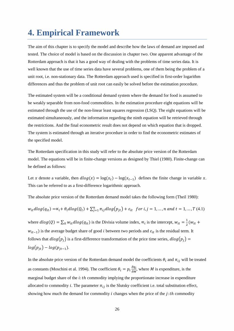
4. Empirical Framework

The aim of this chapter is to specify the model and describe how the laws of demand are imposed and

tested. The choice of model is based on the discussion in chapter two. One apparent advantage of the

Rotterdam approach is that it has a good way of dealing with the problems of time series data. It is

well known that the use of time series data have several problems, one of them being the problem of a

unit root, i.e. non-stationary data. The Rotterdam approach used is specified in first-order logarithm

differences and thus the problem of unit root can easily be solved before the estimation procedure.

The estimated system will be a conditional demand system where the demand for food is assumed to

be weakly separable from non-food commodities. In the estimation procedure eight equations will be

estimated through the use of the non-linear least squares regression (LSQ). The eight equations will be

estimated simultaneously, and the information regarding the ninth equation will be retrieved through

the restrictions. And the final econometric result does not depend on which equation that is dropped.

The system is estimated through an iterative procedure in order to find the econometric estimates of

the specified model.

The Rotterdam specification in this study will refer to the absolute price version of the Rotterdam

model. The equations will be in finite-change versions as designed by Thiel (1980). Finite-change can

be defined as follows:

Let denote a variable, then defines the finite change in variable .

This can be referred to as a first-difference logarithmic approach.

The absolute price version of the Rotterdam demand model takes the following form (Theil 1980):

∑ ( ) (4.1)

where ∑ is the Divisia volume index, is the intercept,

is the average budget share of good between two periods and is the residual term. It

follows that ( ) is a first-difference transformation of the price time series, ( )

( ) .

In the absolute price version of the Rotterdam demand model the coefficients and will be treated

as constants (Moschini et al. 1994). The coefficient

, where is expenditure, is the

marginal budget share of the commodity implying the proportionate increase in expenditure

allocated to commodity . The parameter is the Slutsky coefficient i.e. total substitution effect,

showing how much the demand for commodity changes when the price of the commodity

27

changes. It follows from chapter two that the constant parameters are a weakness of the Rotterdam

approach.

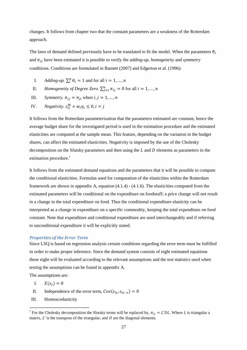
The laws of demand defined previously have to be translated to fit the model. When the parameters

and have been estimated it is possible to verify the adding-up, homogeneity and symmetry

conditions. Conditions are formulated in Barnett (2007) and Edgerton et al. (1996):

I. Adding-up. ∑ and for all

II. Homogeneity of Degree Zero. ∑ for all

III. Symmetry. when

IV. Negativity.

It follows from the Rotterdam parameterization that the parameters estimated are constant, hence the

average budget share for the investigated period is used in the estimation procedure and the estimated

elasticities are computed at the sample mean. This feature, depending on the variation in the budget

shares, can affect the estimated elasticities. Negativity is imposed by the use of the Cholesky

decomposition on the Slutsky parameters and then using the and elements as parameters in the

estimation procedure.1

It follows from the estimated demand equations and the parameters that it will be possible to compute

the conditional elasticities. Formulas used for computation of the elasticities within the Rotterdam

framework are shown in appendix A, equation (4.1.4) - (4.1.6). The elasticities computed from the

estimated parameters will be conditional on the expenditure on foodstuff; a price change will not result

in a change in the total expenditure on food. Thus the conditional expenditure elasticity can be

interpreted as a change in expenditure on a specific commodity, keeping the total expenditure on food

constant. Note that expenditure and conditional expenditure are used interchangeably and if referring

to unconditional expenditure it will be explicitly stated.

Properties of the Error Term

Since LSQ is based on regression analysis certain conditions regarding the error term must be fulfilled

in order to make proper inference. Since the demand system consists of eight estimated equations

these eight will be evaluated according to the relevant assumptions and the test statistics used when

testing the assumptions can be found in appendix A.

The assumptions are:

I.

II. Independence of the error term,

III. Homoscedasticity

1 For the Cholesky decomposition the Slutsky terms will be replaced by, . Where is triangular a

matrix, is the transpose of the triangular, and are the diagonal elements.

28

IV. .

Assumption I implies that the model has been properly specified. If the expected value of the error

term is not equal to zero it implies that the variation in the dependent variable is being captured by the

error term, i.e. there are missing variables that should be added to the model. By plotting the residuals

it is possible to get an opinion on what the expected value is. It follows that the plotted residuals

should not follow any clear pattern. It is also possible to validate this assumption by following,

∑ . If the sum of the residuals is approximately zero the expected value will

also be zero.

Assumption II, independence of the error term, implies that there should be no autocorrelation

between the error terms for the same equation in time, i.e. there should be no correlation between the

error term of and . Correlation can still occur between error terms for different equations,

. Autocorrelation will show when plotting the residuals, or can be formally tested

using the Durbin-Watson (DW) test, see equation (4.1.1) in appendix A (Kleinbaum et al. 2008).

always takes a value between 0 and 4, where implies that there is no autocorrelation present.

An acceptable DW value lies between 1,5 and 2,5.

Assumption III, regarding homoscedasticity refers to constant variance of the error terms. The

variance should not increase, when the independent variables increase. If is the dependent variable

then the variance of is the same for any combination of the independent variable (Kleinbaum et al.

2008). Let, be the variance of then:

(4.2)

The assumption of homoscedasticity will be tested using the Lagrange-multiplier (LM)

heteroscedasticity test, see equation (4.1.2) in appendix A.

Assumption IV, refers to the distribution of the error term, which should be normally distributed. If

the normality assumption holds the estimated parameters will also be normally distributed. The need

for the normality assumption is however only necessary conducting hypotheses testing (Kleinbaum et

al. 2008). Testing for normality is done by the use of the Jarque-Bera (JB) test statistic for regression

analysis, equation (4.1.3) in appendix A.

4.1 Separability in the Rotterdam Model In the scope of the Rotterdam model the verifiable separability condition discussed in chapter three,

takes the following form, (Moschini et al. 1994):

(4.3)

29

where is the budget share. It is now possible to express equation (3.22) in terms of the Rotterdam

parameterization which is testable.

(4.4)

If this restriction holds it locally, it will also be true in the Rotterdam case, for the complete demand

system, hence this make the notion of separability easier to verify compared to other demand systems

(Moschini et al. 1994). In this case , yielding

. It follows that these restrictions will be

imposed on the parameters when conducting the tests of the different utility structures.

4.2 Model Testing and Specifications

When estimating the Rotterdam demand system for this study it is done in several steps. This allows

for testing the regularity restriction which will be imposed on the model. Thus this section will provide

an overview of how the restrictions are imposed on the model and how they will be tested, as well as

the different utility structures.

Formally testing the laws of demand through the use of statistical testing methods is conducted in

order to verify if the conditions and the specification of the model fits the data set. To make sure the

conditions have been correctly specified in the model, the specifications of the laws of demand and the

estimated elasticities can be used. It then follows that when comparing two different model

specifications, either by imposing an economic assumption or a different utility structure, the

likelihood-ratio test is an appropriate test statistic (Moschini et al. 1994). Comparison is then done for

an unrestricted model and a restricted model. The restricted model must be a transformation or special

case of the unrestricted model. This implies that the unrestricted model will always fit the dataset

better compared to the unrestricted model, since it has a more complex specification. The question is

however if the difference is statistically significant. If there is not a statistically verified difference the

restricted model is satisfactory. The standard likelihood ratio test has the following form (Hall and

Cummins 2009):

(4.5)

where is the observed likelihood ratio value, and are the log-likelihood values for the null

and alternative hypothesis respectively i.e. the two different specifications, is degrees of freedom

and is the significance level. The likelihood ratio test follows the chi-square distribution with

degrees of freedom equal to the number of restrictions imposed. The standard likelihood ratio test has

however been shown to be biased towards rejection when dealing with demand systems with many

parameters (Moschini et al. 1994). The alternative formulation of the likelihood ratio test as suggested

30

in Moschini et al. (1994) has the following form, let be the new observed value of the likelihood

ratio test:

[

] (4.6)

where is the number of equations, is the number of observations in the time series. refers to

the number of parameters in the restricted model and is the amount of parameters in the

unrestricted model. is the observed likelihood ratio value of the standard test as defined in equation

(4.5). In this study the both and will presented.

Model Specifications

The hypotheses tested will refer to the conditions imposed on consumer demand, i.e. the regularity

conditions, adding up, homogeneity of degree zero, symmetry and negativity of the Slutsky

substitution matrix. Which specification that is referred to as the unrestricted model will change

depending on which specific condition that is being tested. This is due to the estimation procedure,

where first homogeneity is imposed and compared to the unrestricted specification, where only adding

up is satisfied due to the estimation process. When testing for symmetry however, the specification

where adding up and homogeneity are imposed will be the unrestricted model in the testing procedure.

Thus testing is conditional, on the previously imposed restriction. The different specifications will

therefore be named in the following manner:

Table 4.1. Overview of Model Specifications

Model Name Restrictions Imposed

Specification A Unrestricted

Specification B Homogenous of degree zero

Specification C Homogenous of degree zero

Symmetry

Specification D Homogenous of degree zero

Symmetry

Negativity

The specifications are done in accordance with conditions I, II, III and IV in chapter four.

Utility Structures

When computing the elasticities and imposing the regularity conditions the following utility structure

will be assumed, ). Where ,

, , , ,

31

, , and

The utility structure therefore assumes ad hoc that the consumption of

foodstuff is weakly separated from the consumption of non-food commodities.

The utility structures which will be tested is focused on the food demand.

[ ]

[ ]

The utility structure refers to the case where commodity group meat is assumed to be separable

from the other commodity groups. assumes a utility structures where the foodstuff group has been

divided into three separable commodity groups of animal, vegetable-based and beverages products.

The choice of structures is based on what previously have been assumed for the Swedish demand and

what is common to assume in previous studies, e.g. is similar to the second level of the utility tree

in Edgerton et al. (1996). Formal testing is necessary in order to verify that these structures actually fit

the Swedish demand for food and if they still are appropriate.

Testing the utility structures is done by imposing the restrictions, in the estimation procedure, as

outlined in chapter 4.1. Then the likelihood-ratio value is computed in order to evaluate if they are

appropriate for the Swedish demand for food. Testing of separability is done using specification C, i.e.

symmetry and homogeneity will be the maintained hypothesis. Thus there will be no elasticity

estimates since negativity cannot be ensured.

32

5. Data

The goal of this chapter is to present the data set used in the study and describe modifications making

the data ready of the estimation procedure, the graphs referred to in this section can be found in

appendix B. This also allows for replicating the study and allows for comparison with previous studies

and future research. By examining the graphs it is possible to evaluate the dataset and, get a first

impression regarding the nature of the Swedish demand for food. The data discussed will refer to

changes in; consumption, conditional expenditure and conditional budget shares. It is most likely true

that there have been changes in tastes within the aggregated group, i.e. consumers might prefer pork

compared to beef however these types of questions lie beyond the scope of the study and are hard to

detect in the aggregate dataset.

5.1 Collection and Modification of Data

Responsible for data concerning the consumption of foodstuff is the Swedish Board of Agriculture

(SBA). There are two types of series available, total consumption and direct consumption. Total

consumption refers to the total amount of foodstuff that is used for human consumption. Therefore it

includes all primary products and processed products directly consumed but also includes the

consumption of primary products and processed products that is consumed by the food industry for

further refining of food, (Eklund and Cahlin, 2012). The series direct consumption refers to total

delivery of foodstuff to private households, collective economy households and home consumption of

industries. The commodities included in the direct consumption series is declared in the same

condition as foodstuff reaches the consumer, (Eklund and Cahlin, 2012). It is therefore the data

covering direct consumption that will be used for this study.

Direct consumption is provided in per capita terms by the SBA. The dataset has been modified in

order to fit the COICOP classification in which the price dataset is constructed. This has been done in

order to make sure that the commodity groups include the same goods. This is possible since the

COICOP classification is done at a higher level of aggregation, and the commodity categories in the

dataset provided by the SBA have the corresponding classification codes that give information

regarding the higher level of aggregation groups they belong to.

Conditional expenditure for each food category used in the study is computed by where is

price, is quantity and represents expenditure. It follows that total conditional expenditure is the

sum of the expenditure on all commodity groups. Changes in expenditure thus reflect variations in

prices or increased demand due to other factors. The value of expenditure is computed by using a set

of price indices for each good.

33

5.2 Analysis of Data

This section will discuss the data and variables used in the estimation procedure. The presented

expenditure index is computed in 1995 years prices. This discussion can be viewed to give a

preliminary evaluation of the trend variable for each commodity group, real per capita expenditure and

per capita consumption will be presented in index form. The figures referred to in this section can be

found in appendix B.

Meat and Fish

In figure 5.1 is the expenditure on meat and fish for the period of interest and figure 5.5 shows the

consumed quantities volume index. It is evident that the expenditure on both fish and meat has moved

in a similar manner during the period 1980-2000. In 2000 a significant drop in the consumption of fish

occurred. This unexpected drop is due to the nature of the data available, where the quality of some

commodities in the aggregated fish group cannot be secured. Fresh fish and shellfish were excluded

from the data set, due to unreliable information (Eklund and Cahlin 2012). However for the period

2000-2007 it seems to be the case that the commodities still included in the fish group has experienced

an increase in expenditure. From the 1990’s the price of meat dropped with approximately 12 % until

2006 and then started to increase. During the same period the average price of foodstuff only dropped

with 2 %, thus meat has become relatively cheaper, explaining to some extent the increased meat

consumption (Eidstedt et al. 2009).

Conditional budget shares for meat and fish are presented in figure 5.8. While the budget share for fish

has remained around 2 % annually throughout the entire period, the budget share for meat has

increased with around 1 % during the investigated period to approximately 8, 8 % at the last value.

As there is a noticeable change in the per capita consumption, figure 5.5, for meat in the 1990’s, a part

of the increase can be attributed to changes in agricultural policy and meat products becoming

relatively cheaper (Eidstedt et al. 2009). The total consumption of meat started to increase in the

1990’s and stopped to increase in 2004 and have stayed at the same level for the rest of the researched

period. This could also be viewed in the figure for expenditure where the curve shows an increasing

pattern.

Bread and Cereal Products

In appendix B, figure 5.1 show changes in expenditure for bread and cereal products and in figure 5.8

the budget shares can be found. Per capita consumption is found in figure 5.5. During the period 1980-

1990 the expenditure on bread and cereal products increased. During the 1990’s the expenditure on

bread and cereal products experienced a decrease. The drop in expenditure can be attributed to the

change in agricultural policy during the 1990’s (Eidstedt et al. 2009). The budget shares however have

34

shown an increasing trend and is at the end of the period at 12 % compared to 9,8 % in 1980. This is

verified by the increase in per capita consumption of bread and cereal during the same period.

In the late 2000’s the consumption and expenditure of bread and cereal products increased. The

increase in expenditure can be attributed to both increased consumption and increased prices. It is thus

interesting to note that the real price increase did not offset consumption, i.e. one expects consumption

to decrease when the price increases.

Milk, Cheese and Eggs

Figure 5.2 in appendix B shows the expenditure on milk, egg and cheese products while the budget

shares are found in figure 5.9. Examining the graph shows that expenditure on the commodity group

remained fairly constant in the beginning of the 1980’s, and then increased in the last years of the

1980’s. For the rest of the investigated period the expenditure decreased until it leveled out in 1996,

and have remained at the same level. Examining the consumed quantity index in figure 5.6, the graph

shows a slowly decreasing trend. Thus for periods where expenditure increased, the price must also

have increased. Examining the budget shares shows that the commodity group milk, cheese and eggs,

have the largest budget share compared to all other groups. However the trend is negative and in 2005

milk, cheese and eggs, is passed by fruit and vegetables, which become the largest commodity group

in terms of budget shares. Figure 5.9 shows that the budget shares have decreased from 25 % to 20 %

since the beginning of the period.

Oil and Fats

In figure 5.2, is the evolution of expenditure on oil and fats. This commodity group has also

experienced the same trend in expenditure as is common in several other groups up until 1990’s. The

period following 1990 until 2002 the group experienced a downward trend in expenditure. However

after the 2002 the consumption started to increase again and thus the expenditure on the aggregate

commodity group. The consumption of oils has increased slightly from 2002, as depicted in figure 5.6.

From 2009 and forward there are signs of a positive trend for the expenditure on oil and fats, as well

as per capita consumption. The budget share, figure 5.9, has experienced a negative trend from the

beginning of the period until 2002 and has remained constant for the remaining part of the period.

Hence it is plausible to assume that the increased expenditure can to some extent be attributed to an

increase in demand. In the end of the period the graphs shows what might be the beginning of an

increasing consumption trend.

Fruit and Vegetables

Figure 5.2 in appendix B shows the development of expenditure on fruit and vegetables. Worth noting

is also that included in this commodity group are also potato products such as potato chips and a small

share frozen potato products. From 1980-1987 the commodity group follows the same increase in

35

expenditure as is common in the other commodity groups previously discussed. The following period,

1987-1995 the expenditure decreased but for the remaining period the expenditure has increased.

Throughout the period the consumption of fruit and vegetables has showed a positive trend, see figure

5.6. This is an expected sign, since one would expect the consumption to increase when the price

decreased.

The budget share for the fruit and vegetables commodity group, figure 5.9, shows a negative trend

until 2000 where it starts to increase, and in 2005 the commodity group becomes the largest group in

terms of budget shares. Larger budget shares, increased expenditure and increased per capita

consumption could be viewed as a sign of a change in tastes or habits.

Sweets and Ice cream

The expenditure on sweets and ice cream can be found in figure 5.2 and in figure 5.9 the budget share

is displayed. Expenditure shows the increasing general trend until the 1990’s. After the decreases in

the 1990’s the per capita expenditure has remained somewhat constant. Per capita consumption can be

found in figure 5.6, and the graph depicts a downward sloping trend. The budget share however is

constant throughout the period of interest.

Other Foodstuff

The category other foodstuff contains commodities which are difficult to include in the other groups, it

might therefore be of interest to list the included commodities. Included in the category are:

Pickled herbs

Soups and stock made on animalia and vegetabilia

Dry sauces

Spices

Salt

The commodities included in this group consist mainly of taste enhancers, and products which can be

used as complements. The pickled herbs and dry sauces are responsible for the substantial increase of

the commodity groups. The expenditure on other foodstuff can be found in figure 5.3, and it shows that

expenditure has increased significantly. The same is also true for the per capita consumption in figure

5.7, for this category. The budget share shows a positive trend, figure 5.10. It is worth noting when

dividing the commodity groups when testing for separability, this group will be viewed as vegetabilia.

Some animal products can be found in the soup category, which is included in the in this food group,

however the share of soups of the whole other food category is relatively small, around 10 %. It

follows that of the 10 % soup share there are soups with animal products, however it is not possible to

distinguish between these two in the data set.

36

Alcoholic and Non-Alcoholic Beverages

Expenditure on alcoholic beverages follows shows a positive trend from the beginning of the period

until 1990, figure 5.3. For the remaining period real expenditure on alcoholic beverages has remained

fairly constant. Non-alcoholic beverages show signs of increased and decreased expenditure until 1992

and have for the remaining period experienced an increase. Interesting is though that the per capita

consumption of alcoholic beverages, figure 5.7 increased until the early 1990’s, but have for the

remaining period been constant.

The budget share in figure 5.10 shows that for alcoholic beverages, the share increased from the

middle of the 1980’s until the beginning of 2000. After 2000 the trend became downward sloping and

the budget share decreased for the remaining part of the period. The share of expenditure on non-

alcoholic beverages have in the long-run increased during the period, however the amount spent

experiences some sort of volatility.

Concluding Remarks

The development of the total conditional expenditure of food is shown in figure 5.4. It is evident that

at a higher aggregated level the real expenditure on food is at the same level as in the beginning of the

period. Since the initial relatively higher price level in the 1990’s dropped, there is a positive trend

showing increased expenditure. The total budget share spent of food commodities has decrease to

around 10-15% from around 20%, note that this is not a conditional budget share (Eidstedt et al.

2009). This implies that relative to the consumption of other non-food commodities the budget share

of foodstuff has decreased. This is to be expected since foodstuff is usually viewed as a necessity and

after a while a consumer stops demanding more food as wealth increases. The general pattern that

expenditure showed decreases after the 1990’s could be attributed to the change in agricultural policy

and the fact that the relationship between the general price level in the economy and the price level of

food stuff changed implying that food became relatively cheaper compared to non-food (Eidstedt et al.

2009).

It follows from the data analysis that the commodity group fish will not be included in the estimation

procedure due to the unreliable dataset. Since the goal was to try to depict a complete set of

commodities a consumer might face, this is not completely possible anymore. Inclusion of unreliable

data will have impact on the result, and should be avoided. This is unfortunate since fish could be

viewed as a substitute to meat, and it could be the case that some variation is not unaccounted for.

Therefore only nine equations will be included in the demand system.

It is evident that there in some cases there have been significant changes in the budget shares. The

notion of budget share is an important concept in the Rotterdam model and it might be the case that

the changes in share will affect the resulting elasticities.

37

6. Results and Discussion

In this section the result of the estimation procedure and the statistical performance of the Rotterdam

model will be presented and discussed. This section will begin with an analysis of the residuals and

then evaluating the regularity conditions imposed on the Rotterdam model and finally report and

discuss the economic results of model.

6.1 Residual Diagnostics

Residual plots can be found in appendix D for all eight estimated equations, figure 6.1 – 6.8 and the

test values for the different test statistics in appendix C.

Table 6.1. Overview of Test Results

Commodity Equation No

Autocorrelation

Homoscedastic Normally

Distributed

Bread and Cereal Equation 1 X X X

Meat Equation 2 X X X X

Milk, Cheese and Eggs Equation 3 X X X*

Oil and Fat Equation 4 X X X X

Fruit and Vegetables Equation 5 X X X X

Other Foodstuff Equation 6 X X X X

Non-Alcoholic Beverages Equation 7 X X X X

Alcoholic Beverages Equation 8 X X X X*

In table 6.1 above is an overview of the results of the residual diagnostics for the eight estimated

equations. Equation nine is not estimated, the parameters are retrieved through the restrictions

imposed. Hence diagnostic is only possible for the eight estimated equations. Diagnostic evaluation is

conducted when all the regularity conditions have been imposed. An X implies that the assumption is

satisfied. Description of the tests can be found in chapter four.

By summing over the residuals, for each respective equation, it is evident that the expected value for

all residuals equals zero. It follows from ∑ . It can also be verified by looking

at the residuals plotted in appendix D. Residuals are located both on the positive area and the negative

area of the plot which indicates an expected value tending towards zero.

From the DW test it is confirmed that there is no autocorrelation present, see table 6.1.1 in appendix C,

for the DW values which are all in an acceptable range. An acceptable range refers to a DW value

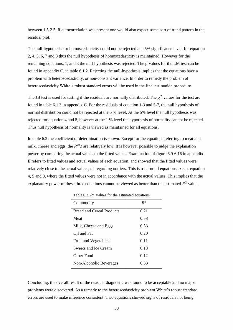
38

between 1.5-2.5. If autocorrelation was present one would also expect some sort of trend pattern in the

residual plot.

The null-hypothesis for homoscedasticity could not be rejected at a 5% significance level, for equation

2, 4, 5, 6, 7 and 8 thus the null hypothesis of homoscedasticity is maintained. However for the

remaining equations, 1, and 3 the null-hypothesis was rejected. The p-values for the LM test can be

found in appendix C, in table 6.1.2. Rejecting the null-hypothesis implies that the equations have a

problem with heteroscedasticity, or non-constant variance. In order to remedy the problem of

heteroscedasticity White’s robust standard errors will be used in the final estimation procedure.

The JB test is used for testing if the residuals are normally distributed. The values for the test are

found in table 6.1.3 in appendix C. For the residuals of equation 1-3 and 5-7, the null hypothesis of

normal distribution could not be rejected at the 5 % level. At the 5% level the null hypothesis was

rejected for equation 4 and 8, however at the 1 % level the hypothesis of normality cannot be rejected.

Thus null hypothesis of normality is viewed as maintained for all equations.

In table 6.2 the coefficient of determination is shown. Except for the equations referring to meat and

milk, cheese and eggs, the are relatively low. It is however possible to judge the explanation

power by comparing the actual values to the fitted values. Examination of figure 6.9-6.16 in appendix

E refers to fitted values and actual values of each equation, and showed that the fitted values were

relatively close to the actual values, disregarding outliers. This is true for all equations except equation

4, 5 and 8, where the fitted values were not in accordance with the actual values. This implies that the

explanatory power of these three equations cannot be viewed as better than the estimated value.

Table 6.2. Values for the estimated equations

Commodity

Bread and Cereal Products 0.21

Meat 0.53

Milk, Cheese and Eggs 0.53

Oil and Fat 0.20

Fruit and Vegetables 0.11

Sweets and Ice Cream 0.13

Other Food 0.12

Non-Alcoholic Beverages 0.33

Concluding, the overall result of the residual diagnostic was found to be acceptable and no major

problems were discovered. As a remedy to the heteroscedasticity problem White’s robust standard

errors are used to make inference consistent. Two equations showed signs of residuals not being

39

normally distributed at the 5 % significance level, however at the 1 % significance level they could be

said to follow the normal distribution. Some of the are quite low and one would hope for a

greater value, however comparing the fitted and the actual values showed that some equation can be

considered to have a decent explanatory power. Due to the method chosen this is expected, using a

first-difference approach affects the value of negatively. However it does not have to imply that the

equations fail to capture the variations of the variables.

6.2 Model Specification Testing

Testing of the regularity conditions will be done according to the procedure outlined in chapter four,

and the models referred to are specified in table 4.1. Testing for the inclusion of the intercept is also

conducted for each specification in order to acknowledge trend changes and verifying that the

intercept fits the data for each specification.

In table 6.3 below are the log-likelihood values for different specifications with different sets of

conditions imposed, with and without intercept. These values are used when computing the likelihood

ratio.

Table 6.3. Log Likelihood Values

Model Specification With Intercept Without Intercept

Specification A

Specification B

Specification C

Specification D

40

Testing for the Inclusion of the Intercept

In table 6.4 an overview of the test procedure for the inclusion of the intercept is shown. The

likelihood ratio values are computed according to equation (4.5) and (4.6).

There are eight restrictions imposed on each specification yielding the following critical value,

. It is evident that the null hypothesis is rejected at the 5 % significance level for the

specifications A, C and D given or . For specification B the null hypothesis cannot be rejected

at the 5 % significance level while using the test statistic, but with the standard test statistic the

null hypothesis would be rejected. Three of four specifications showed that the intercept should be

included, and the standard likelihood-ratio value implied for specification B that the intercept should

be included. It follows that when testing for the regularity conditions, the intercept will be included for

each specification. The interpretation of the intercept term is thus; when the variation in price and

expenditure is zero, the value of the intercept will be the variation in the quantity demanded. Therefore

it can be interpreted as changes in non-economic factors. The statistically significant intercept terms

will imply which equations trend changes are present. In table 6.1.4 in appendix C, the intercept

estimates can be found. Of eight estimated intercept terms five estimates were statistically significant

at some level implying that there have been trend changes for the following equations, 2, 3, 6, 7 and 8.

The value of the intercept for equation nine is retrieved through ∑ .

Table 6.4. Testing for the Inclusion of the Intercept

LR

Specification A

Without intercept

With intercept

Specification B

Without intercept

With intercept

Specification C

Without intercept

With intercept

Specification D

Without intercept

With intercept

41

Testing the Laws of Demand

The hypotheses formulated below can be interpreted as testing the imposed laws of demand, as

outlined in chapter four. The observed likelihood ratio values are given in table 6.5. Testing is done

conditional on each specification, e.g. symmetry will be tested conditional on imposing homogeneity.

Test 1 has 8 restrictions, hence 8 degrees of freedom due to the formulation of the homogeneity

constraint, thus the critical value is . The likelihood ratio value using both test statistics

indicates that the null hypothesis cannot be rejected. Using indicates that at the 5 % level the null

hypothesis is just barely maintained. However as previously discussed, the standard test statistic has a

tendency to over reject the null hypothesis. It follows from alternative test statistic, , indicates that

the hypothesis is can be maintained at the 5 % level with more confidence.

Test 2 has 28 degrees of freedom. It follows from the total amount of parameters, , which are 64,

of which eight are unique parameters, for the eight estimated equations. This leaves 56

parameters which are assumed to be symmetric, yielding 28 restrictions. Thus is the

critical value. Therefore the null-hypothesis cannot be rejected in favor of the alternative hypothesis at

the 5% significance level. It follows that conditional on homogeneity the hypothesis of symmetry is

maintained.

Test 3, tests negativity of the Slutsky matrix conditional upon homogeneity and symmetry. The

specification has, homogenous of degree zero, symmetry and negativity imposed. The critical value is

. Five degrees of freedom follows from the five restrictions from the estimation

procedure where only three of eight elements of the Choleksy decomposition are used. The

observed likelihood ratio value is smaller than the critical value at the 5 % significance level implying

that the null hypothesis cannot be rejected. Thus conditional on homogeneity and symmetry, imposing

Table 6.5. Testing Laws of Demand

LR

Test 1 Homogeneity

Homogenous of Degree Zero

Not Homogenous of Degree Zero

Test 2 Homogeneity and Symmetry

Homogenous and Symmetric

Homogenous

Test 3 Homogeneity, symmetry, and negativity

Homogenous, Symmetric, Negativity

Homogenous and Symmetric

42

negativity yields a model which does not have a worse fit than the previous specifications even though

several restrictions have been imposed.

Concluding Remarks

Testing the regularity conditions are done in order to get estimates that are consistent with economic

theory and verify that the data fit the imposed restrictions. It is necessary to either impose the

regularity conditions if they are not spontaneously fulfilled. It was only possible to use three

elements of the Cholesky decomposition in the final estimation due to non-linearity in formulating the

negativity constraints, and at the same time achieve convergence of the estimation procedure.

Including more elements would yield a higher log-likelihood value, however the value can only

improve up to the value of specification C. Since the difference between the log-likelihood of

specification C and D is small it is plausible to assume that including more elements would not change

the outcome, the hypothesis of negativity would still be maintained. The test procedure showed that

the hypothesis of the laws of demand can be maintained and specification D will be used for the

elasticity estimates. The choice of test statistic did not influence the result. The null hypothesizes for

the different specifications could be maintained using the standard test statistic. However for test 1 the

hypothesis was barely maintained due to the tendency of over rejecting, but the alternative test

statistics indicates that the null hypothesis can be confidently maintained.

6.3 Economic Results

6.3.1 Elasticities In table 6.6 the conditional expenditure elasticities are presented. Complete conditional elasticity

matrices can be found in appendix F. All elasticities are computed at the sample mean. From the

estimation procedure it was found that the commodities, bread and cereal products, milk, cheese and

egg, non-alcoholic beverages and alcoholic beverages can be classified as luxury commodities by

having expenditure elasticity greater than 1. The remaining commodities, meat, sweets and ice cream

and other food, were found to be necessary goods, while oil and fat and fruit and vegetables classified

as inferior goods.

Table 6.6. Conditional Expenditure Elasticities

Commodity Expenditure Elasticities Classification

Bread and Cereal Products 1.7243*** Luxury

Meat 0.9790** Necessity

Milk, Cheese and Eggs 1.8750*** Luxury

Oil and Fat -1.3450*** Inferior

Fruit and Vegetables -0.0989 Inferior

Sweets and Ice Cream 0.6023 Necessity

Other Food 0.8873 Necessity

Non-Alcoholic Beverages 2.0266*** Luxury

Alcoholic Beverages 1.1681*** Luxury Significance level, 10%=*, 5%=** ,1%=***

43

Table 6.7 contains both the Marshallian and the Hicksian conditional own-price elasticities. Of the

Hicksian own-price elasticities seven were found to be statistically significant while for the

Marshallian 6 were found to be significant. All of the commodities have negative own-price

elasticities satisfying the negativity condition. From the values of the elasticities, i.e. they are between

-1 and 0, it is evident that all commodities can be classified as having a relatively inelastic demand.

From the relationship between the Hicksian and Marshallian elasticities, the Marshallian elasticity

should be larger in absolute value than the Hicksian, or vice versa if the commodity is classified as an

inferior good. Examining the complete elasticity matrix in table 6.1.5 and 6.1.6 in appendix F, shows

that this relationship is satisfied for both own-price and cross-price elasticities. The commodities

which were classified as inferior show the inverse relationship and thus have a Marshallian elasticity

that is greater than the Hicksian.

Table 6.7. Conditional Own-price Elasticities

Commodities Hicksian Marshallian

Bread and Cereal -0.0549 -0.2529

Meat -0.5523*** -0.6328***

Milk, Cheese, Egg -0.2096* -0.6383***

Oil and Fat -0.1840 -0.0934

Fruit and Vegetables -0.2012* -0.1800

Sweets and Ice Cream -0.2380*** -0.2699***

Other Food -0.7871*** -0.8148***

Non-alcoholic Beverages -0.1337** -0.3726***

Alcoholic Beverages -0.4555** -0.5616** Significance level, 10%=*, 5%=** ,1%=***

Classification of substitutes and complements is done by the use of the cross-price elasticities. Of the

Hicksian cross-price elasticities both net substitutes and net complements were found. 25 net

complementary goods were found and the other 47 cross-price elasticities indicate net substitutes.

From the Marshallian elasticity matrix 47 gross complements and 25 gross substitutes were found. The

statistically significant Marshallian cross-price elasticities show only a few substitution goods. All the

statistically significant substitutes were found to the commodity group oil and fats, disregarding the

case that meat classified as a substitute to alcoholic beverages. The remaining statistically significant

elasticities classified as gross complementary commodities.

By using the restrictions specified in chapter 3.3 on the estimated elasticities, it can be verified that the

imposed regularity conditions have been correctly specified and implemented. If they do not hold it

would imply some misspecification.

6.3.1 Utility Structures

Table 6.8 shows the likelihood ratio values of the two utility structures tested . The critical

values are given according to the amount of restrictions imposed on the structures. The restrictions are

formulated according to equation (4.4). For the degrees of freedom are yielding a critical value

44

of , and for with 17 degrees yields

. It is evident that none of the

separability structures imposed on the demand for food is rejected. The same conclusion is reached by

the two different test statistics, and . It therefore follows that it is plausible to assume that the

consumption decisions of meat are weakly separable from the other commodities. The same is true for

the structure , implying weak separability between the three aggregated commodity groups

specified.

Table 6.8. Testing of Separability Structures

Hypothesis

Separability of meat

Meat is not separable

Separable according to

Not separable according to

6.4 Discussion The estimated elasticities are to some extend a result of the restrictions imposed and the functional

form used, hence it is necessary to discuss these properties. The restrictions imposed are done in order

to make sure the results are consistent with microeconomic theory, i.e. the laws of demand are

maintained for the estimates. Some of the results can be viewed as slightly unusual in the context of

economic theory, e.g. the classification of two commodity groups as inferior goods, which is still

possible even though the regularity conditions are imposed. Due to the choice of a conditional demand

system, the result have some limitations, but through the use of estimates made by Seale et al. (2003)

and (2011) it is possible to compute crude approximations of unconditional expenditure and

Marshallian elasticities as shown in table 6.4.1 and 6.4.2. The limitations follow from the fact that the

group expenditure are assumed to be constant when estimating a conditional demand system. Hence

the classification of the commodities using the conditional expenditure elasticities can only be seen as

within group classification. Computation of the unconditional Hicksian elasticities is not as straight

forward and will therefore not be included.

6.4.1 Significance

Unfortunately relatively few of the estimated Hicksian price elasticities are statistically significant; 18

of the Hicksian and 36 of the Marshallian price elasticities were found significant at some level. One

possible explanation to this is the use of several prices as variables. It is expected that price of different

food commodities are correlated with each other, and thus reducing the number of significant

parameters in the estimated model. One could remedy this with removing one of the variables which

one expects to capture the same variation as another variable. Removing prices is however not

preferred in demand system analysis. Theoretically it would mean that the commodity does not depend

on the price which is being removed. And this is thus one trade-off which has to be made, comparing

45

statistical performance with economic theory. Otherwise the overall the statistical performance of the

model is acceptable.

The examination of the Marshallian price elasticities showed that relatively more of the estimates are

significant. It follows from the computation of the Marshallian compared to the Hicksian, see equation

(4.1.4) – (4.1.6) in appendix A, where more information is available for the computation of the

Marshallian price elasticities i.e. the expenditure elasticity is also included. Thus the information

contained in the expenditure elasticity influence the significance of the Marshallian estimates.

6.4.2 Trend Effects

It is possible to some extent acknowledge trend changes. Testing for the inclusion of the intercept

showed that it should be included in the demand system. Trend changes can then be said to have

occurred for the commodities that have a statistically significant intercept. Meat, milk, cheese and

eggs, sweets and ice cream, other foodstuff and non-alcoholic beverages, had significant intercepts;

meat, other foodstuff and non-alcoholic beverages had positive intercepts while equations milk, cheese

and eggs and sweets and ice cream had negative intercepts. This implies that there have been positive

and negative trends present during the investigated period i.e. variations which cannot be attributed to

changes in price or expenditure. It is possible that these changes can be attributed to the non-economic

factors discussed in chapter two, unfortunately it is not possible to distinguish which factors that have

changed without a more detailed model. As discussed in chapter five, meat, other food and non-

alcoholic beverages had showed signs of positive trends in the consumption and expenditure diagrams

while milk, cheese and eggs and sweets and ice cream, had shown signs of a negative trend. This can

thus be confirmed by the estimated intercept terms that indicate the same pattern.

6.4.3 Price and Expenditure Elasticities

From the presented Hicksian elasticity matrix, appendix F, it is evident that some unusual substitutes

are observed i.e. commodities which do not fulfill the same goal. For the Hicksian cross-price

elasticities it could be the case that when the price of a commodity increases and a consumer is

supposed to keep the utility constant, consumption of goods which does not immediately fulfill the

same purpose is consumed and therefore yielding unexpected substitutes. Since consumption of any

good increases utility, it is not certain that a consumer will shift to a commodity which should be a

substitute, and thus unexpected substitutes are observed.

The estimated Hicksian cross-price elasticities have relatively small values. The largest Hicksian

cross-price effect (0.43) is between other food and milk, cheese and egg. Both net and gross

substitution and complementary effects are observed, they are however to be considered relatively

small. As discussed in the chapter three the Hicksian price elasticities refers only to substitution

effects, while the Marshallian accounts for both the income effect and the substitution effect. Hence

the Hicksian price elasticity can be viewed as a movement along an indifference curve. From the

46

properties of the Hicksian price elasticity, the nature of classifying goods as complements or

substitutes should not change which can occur for the Marshallian elasticities. This property is an

effect of the symmetry conditions, implying theoretically that the order in which the second-order

derivatives are taken does not matter. In the Rotterdam parameterization it follows from , and

thus the Slutsky terms are the same. The value can however be different depending on the budget

share of each respective commodity. In the presented Marshallian elasticity matrix it is the case that;

consumers view more commodities as complementary compared to the Hicksian. The classification of

commodities can also change, e.g. milk, cheese and eggs are viewed as a gross substitute to meat

while meat is viewed as a gross complement to milk, cheese and eggs, while they are both viewed as

net substitutes. Therefore the Hicksian elasticities are better for deciding the nature of complements

and substitutes between commodities since the order in which one looks at the commodities does not

matter, and when one is interested in the gross effect on the demanded quantity the estimated

Marshallian elasticities should be used. The change in classification between Marshallian and

Hicksian elasticities is due to the fact now the consumer adjusts taking into account the effect of the

real income change and this crowds out the substitution effect. Thus the Hicksian indicate more

substitutionary goods.

The result of analyzing the conditional own-price elasticities is consistent according to the laws of

demand stating that they should be negative, i.e. as the own price increases the quantity demanded

decreases. If it was the case that the estimates should not be according to microeconomic theory, the

specification testing i.e. test three, would reject the hypothesis of negativity implying that the data

does not fit the conditions imposed and then positive own-price elasticities could be observed. The

estimated Marshallian and Hicksian conditional own-price elasticities are classified as inelastic which

indicates that the consumers are insensitive to own-price changes, i.e. if the price increases, the

decrease in the quantity demanded is expected to be relatively small. It follows that the Swedish

demand for food is inelastic and insensitive to price changes. However the range of the values

indicates that there are commodities which can be viewed as relatively more inelastic e.g. the group

bread and cereal products have a Hicksian own-price elasticity which is relatively close to zero,

indicating that the change in demand due to a change in the own price will be small. While other food

commodities have a relatively more elastic compared to bread and cereal, due to the own-price

elasticity being further from zero. It follows from the Hicksian elasticities that bread and cereal have

the most inelastic demand while the group, other food is relatively most elastic. The same reasoning is

true for the Marshallian elasticities, disregarding the inferior commodities.

Due to the limitations of the conditional elasticities it is of interest to see how much they differ from

the unconditional. Computing the unconditional elasticities will strengthen the conclusion regarding

the sensitiveness of the demand even though they are approximations. Through the use of Seale et al.

(2011) estimates of the own-price elasticity for aggregate food it is possible to give a crude

47

approximation of the unconditional Marshallian own-price elasticity.2 In some cases the changes are in

the elasticity value is significant. The greatest differences occur for the commodities with the greatest

conditional expenditure elasticities. The general classification of the demand as inelastic to price

changes is however the same. This indicates that the classification of inelastic or elastic commodities

using own-price elasticities from a conditional approach gives a plausible conclusion. The general

effect is that the unconditional elasticities indicate that the demand becomes less elastic i.e. the

conditional ones are larger in absolute value than the unconditional elasticities. It is evident that when

using the unconditional Marshallian own-price elasticities all commodities are viewed as inelastic and

that the Swedish demand for food is insensitive to own-price changes. The relationship of the relative

inelasticity is the same as for the conditional Marshallian; bread and cereal has the most inelastic

demand while other food has the least inelastic demand disregarding the inferior goods (fruit and

vegetables and oil and fats). This indicates that the relationships between the normal goods are not

affected by the conditional approach. For the inferior commodities the relationship is reversed, the

unconditional are larger in absolute value compared to the conditional.

Table 6.9 Unconditional and Conditional Own-Price Elasticities

Commodities Unconditional Marshallian

Own-Price Elasticities

Conditional Marshallian

Own-Price Elasticities

Bread and Cereal -0.1417 -0.25293

Meat -0.5876 -0.63282

Milk, Cheese, Egg -0.3974 -0.63826

Oil and Fat -0.1443 -0.09338

Fruit and Vegetables -0.1919 -0.18004

Sweets and Ice Cream -0.2520 -0.26991

Other Food -0.7992 -0.81476

Non-alcoholic Beverages -0.2383 -0.37261

Alcoholic Beverages -0.5019 -0.56163

From the estimated conditional expenditure elasticities it is possible to classify them as done in table

6.6. However within group classification can be misleading since this classification will not be true for

the unconditional elasticities and does not take into account changes in the allocation of expenditure. It

is expected that the unconditional elasticities will be significantly different since the upper-stage

elasticity for food is usually small. The classification in table 6.6 can thus be viewed as within group

luxuries and necessities. It follows that the interpretation of the conditional elasticities is; how much

the quantity demanded changes due to changes in within group expenditure. Hence one can say which

commodity causes the greatest or smallest changes in demand, keeping group expenditure constant, in

2 Unconditional Marshallian own-price elasticities are computed using (Moschini and Moro 1993):

where is the budge share of good .

is the elasticity for food found in Seale et al. (2011)

48

this case it is non-alcoholic beverages and sweets and ice cream respectively, disregarding the inferior

commodities. One can also compare two commodities and say which is more sensitive than the other.

The relationship regarding which commodity is more or less sensitive will be the same for the

unconditional expenditure elasticity. To be able to find how the sensitive the demand is to changes in

expenditure and allowing for allocation changes, crude computation of the unconditional expenditure

elasticities are shown in table 6.10, in comparison to the conditional ones. These have been computed

using the upper-stage elasticity for the food group as a whole, which have been computed in Seale et

al. (2003). 3 The value used is 0.354 which indicates that the conditional elasticities will be scaled

down. Analyzing the unconditional elasticities shows that all commodities now classify as necessities

or normal commodities with the exception of the inferior goods, which was also the case for the

conditional. Taking into account the upper-stage indicates that the Swedish demand for food is

relatively insensitive to expenditure changes. Hence the expenditure elasticities from the conditional

estimation are not the best suited for classification of the general sensitiveness of demand to changes

in expenditure. Since these are approximates it follows that the values might not be fully

representative, however the classification of the commodities as necessities can be viewed as

plausible.

Table 6.10. Unconditional and Conditional Expenditure Elasticities

Commodities Unconditional Conditional

Bread and Cereal 0.6104 1.7243

Meat 0.3466 0.9790

Milk, Cheese, Egg 0.6637 1.8750

Oil and Fat -0.4761 -1.3450

Fruit and Vegetables -0.0350 -0.0990

Sweets and Ice Cream 0.2132 0.6023

Other Food 0.3141 0.8873

Non-alcoholic Beverages 0.7174 2.0266

Alcoholic Beverages 0.4135 1.1681

The commodity group, oil and fat, and fruit and vegetables are classified as an inferior good according

to both conditional and unconditional expenditure elasticity estimate. This is an unusual result since

the classification of inferior good is somewhat controversial. This implies that as expenditure increases

the quantity demanded will decrease for these two commodities. A negative marginal budget share,

, from the estimation procedure will turn the expenditure elasticity negative due to the framework

used; see equation (4.1.4) in appendix A. The budge share for the oil and fat commodity group has

been decreasing throughout the investigated period which can turn the marginal budget share negative.

It is more unexpected that fruit and vegetables are classified as an inferior good, due to the budget

3 The unconditional expenditure elasticity is a product of the upper-stage elasticity and the conditional expenditure elasticity.

.

is found in Seale et al. (2003).

49

share does not have a clear negative trend. However the elasticity estimate is relatively close to zero

compared to the expenditure elasticity of oil and fats. One possible explanation is also, due to the fact

that the fruit and vegetables commodity group has potatoes included, which has been classified as an

inferior good in previous studies, and could affect the estimate to become negative. It is unfortunately

not possible to distinguish the effect of including the potato in the commodity group. One possible

solution would be to disaggregate and remove potatoes from the commodity group and re-estimate the

model.

As discussed in chapter two, the functional form and the parameterization of the Rotterdam model can

affect the expenditure elasticities. The estimated expenditure elasticities are thus only representable if

the budget shares experience minor variations. The constant nature of the and the functional form,

also influence the estimates in a way which is not consistent, implying; as expenditure increases the

elasticity of necessities increase, since the budget share decreases when prices are kept constant. The

functional form implies that the marginal budget share is smaller than the budget share for the

commodities classified as necessities. For the commodities classified as luxuries it implies that the

estimated marginal budget share is greater than the budget share, hence if expenditure increase, while

prices are kept constant, the expenditure elasticity will decrease. This relationship is not appropriate

for food commodities since it is expected that food should become less of a luxury commodity as

expenditure (income) increases. Hence the great elasticities for some commodities are questionable;

however it is possible to arrive at these due to the conditional approach indication the limitations the

conditional demand systems. For the commodity group non-alcoholic beverages it is the case that the

estimated marginal budget share is significantly larger than the budget share yielding a large elasticity

it follows that the estimated marginal budget share is substantially larger than for commodities with

similar budget shares.

As shown in chapter five only meat and sweets and ice cream have budget shares which can be said to

have minor changes. Since in the computation of the elasticities the sample mean is used, and there are

changes which cannot be viewed as minor for the remaining commodities, the sample mean will not

be accurate for the entire period and is not a good approximation of the budget share. This implies that

a more representative budget share than the sample mean might be better suited for the computation of

expenditure elasticities which have significant changes in budget shares. It is apparent that the

functional form is affecting and the expenditure elasticity. It follows that the estimated expenditure

elasticities are not representable due to changes in budget with the exception of meat and sweets and

ice cream where changes have been minor. If variation in budget shares had been minor for the other

commodities the performance would have been more accurate. The problems with the conditional

expenditure elasticities do not however change the classification using the unconditional elasticities.

Classification of all commodities as necessities, implying an inelastic demand is still plausible since

the upper-stage elasticity is relatively small, if the estimates were more accurate the estimates would

50

be even smaller. The inaccuracy of the expenditure elasticities somewhat transfer to the Marshallian

elasticities, indicated by the large difference for some conditional and unconditional own-price

elasticities, however the general conclusion regarding an inelastic demand is still viable.

6.4.4 Comparison

It is possible to some extent compare the own-price elasticities found in this study to the previous

studies discussed. Comparing the commodity groups which are similar to the study conducted by Lööv

and Widell (2009) shows that general difference is when looking at the conditional Marshallian own-

price elasticities. The elasticities estimated by Lööv and Widell are relatively more elastic, the value is

generally higher. However classification of the goods as inelastic or elastic is the same except for the

commodity group meat, given conditional elasticities. Meat is classified as an elastic good in Lööv and

Widell’s study and in this study the demand for meat is classified as inelastic. Worth noting is that

Lööv and Widell uses Marshallian elasticities for classification of substitutes and complements, thus

the problems regarding the changing nature of commodities is evident. The general substitutionary and

complementary effects which are present in this study are similar to the ones found in Lööv and

Widell (2009), when using Marshallian elasticities. Different classification only occurred in three

cases. Meat was classified as a gross substitute to milk, cheese and egg, and fruit and vegetables while

they were classified as gross complements in this study. Fruit and vegetables were classified as a

substitute to meat in Lööv and Widell (2009), while classified as a complement in this study.

Comparing the results to the study conducted by Edgerton et al. (1996) shows a similar result using the

conditional Marshallian elasticities, the demand can be considered to be inelastic. A difference can be

observed in how inelastic the commodities are. The result from Edgerton et al. (1996) is relatively less

inelastic compared to the result obtained in this study with the exception of milk, cheese and eggs.

Conditional cross-price elasticities are not reported in Edgerton et al. (1996), hence no comparison is

possible. It is interesting to note that their study mostly rejected the laws of demand for the various

demand sub-systems, compared to this study where the hypothesis of the laws of demand could be

maintained.

Due to the nature of the conditional expenditure elasticities it is of more interest to compare the

unconditional found in Edgerton et al. (1996). For the unconditional elasticities the general conclusion

is the same, that the demand is insensitive to expenditure changes disregarding the inferior goods.

Some differing results regarding specific commodities can be observed, meat in Edgerton et al. has an

unconditional elasticity of 0.64 while this study find 0.34. It might thus be the case that the demand for

meat is now relatively more insensitive to expenditure changes. Milk, cheese and eggs are however

found to be relatively more sensitive for changes in expenditure.

The differences in results can to some extend imply that there might have been a change in how the

consumers behave and therefore a change in the classification of certain commodities however a more

51

detailed framework is needed to discuss if there has been a structure break. Still the study conducted

by Lööv and Widell and this study covers to some extent the same time period and produces different

results. It is interesting that they found the demand for meat to be elastic while this study found it to be

inelastic given conditional own-price elasticities. It could be the case that over the recent years the

demand for meat has changed it properties. It also follows that some of the differences between the

result of this study and the other two depends on the functional form used. As discussed in chapter two

the classification of substitutes and complements is problematic with the AIDS approach. The

classifications from the estimated Rotterdam approach do not have this uncertainty.

6.4.6 Utility Structures

Imposing the two different utility structures showed that it is plausible to separate a consumer’s

demand for food according to the two specifications. This result is satisfactory since proper specified

utility structures will allow for more detailed analysis of certain commodity groups and when setting

up a full demand system. Testing for utility structures using a conditional approach will produce

results that will hold for a full or a complete demand system, as mentioned in chapter three, the result

holds globally. As discussed, the test statistic used can to some extend influence the result, and

therefore it was satisfactory that both proposed test statistics could not reject the null-hypothesis of the

specified structures. The construction of a full demand system would allow for more accurate

unconditional elasticities since one does not have to rely on secondary sources.

Unfortunately it is not possible to obtain elasticities from the system with the utility structures

imposed. Negativity is not imposed on the separated systems and thus elasticities would not be

obtained under the same circumstances as the system with negativity imposed i.e. the estimates which

have been presented. Not imposing the proposed separability structures on the estimated elasticities is

due to the complexity when formulating the negativity constraint and it will not be possible to impose

the restrictions referring to the separable structures and the negativity at the same time. Differences in

the estimates could therefore be attributed to the absence of the negativity constraint and thus not only

the different structures. It is therefore not possible to evaluate if the utility structures affect the

estimated elasticities, however it is expected that the structures do change the estimates, see Edgerton

(1997). A different framework or another method for imposing negativity would be necessary. The

result can thus be viewed as verifying two plausible separable structures for the Swedish food demand.

52

7. Conclusion

The aim of this study was to examine the Swedish demand for food over the period 1980-2011, and

analyze how sensitive it is to changes in expenditure and prices. The choice of method was a

conditional Rotterdam demand system approach, assuming that foodstuff is weakly separable from

non-food commodities. In order to cope with the limitations of conditional demand system crude

estimates for the unconditional expenditure elasticities and Marshallian price elasticities were

computed in order to capture the information lost when dealing with conditional estimates. The

demand system eventually consisted of nine commodities which were estimated in order to analyze the

properties of the Swedish food demand. Imposing the laws of demand was done in order to achieve

theoretically consistent result. The hypotheses of the laws of demand were also maintained. The

econometric performance of the estimated demand system was found to be acceptable although a

greater share of statistically significant parameters is desired. Trend effects were observed, indicating

changes in non-economic factors for several commodities. Meat, other food and non-alcoholic

beverages showed a positive trend, while milk, cheese and eggs and sweets and ice cream depicted a

negative trend.

From the analysis of the conditional and the unconditional Marshallian own-price elasticities it is

evident that the Swedish demand for food can be considered inelastic and insensitive to changes in

price. The difference between the unconditional and conditional Marshallian elasticities is large for the

commodities with large expenditure elasticities however the demand is still insensitive to price

changes. The cross-price conditional elasticities showed that there exists, both net and gross,

complementary and substitution effects. These effects are however to be considered relatively minor.

Analysis of the conditional expenditure elasticities showed that some commodities are affected by the

Rotterdam parameterization and therefore the robustness is uncertain. The functional form and the

Rotterdam approach can be said to have influenced the expenditure elasticities leading to inaccurate

estimates. The estimates for sweets and ice cream and meat can however be said to be representative

due to the relatively minor changes in budget shares, and the expenditure elasticities for these indicate

that demand is relatively insensitive to expenditure changes. As discussed a different and more

dynamic functional form could be better suited to compute expenditure elasticities. The unconditional

expenditure elasticities do however indicate that the demand is insensitive to expenditure changes.

Two inferior commodities were observed, fruit and vegetables and oil and fats. Inferior commodities

are rather uncommon and thus this result should be viewed as uncertain.

The study tested two verified utility structures for the Swedish demand for food. The suggested utility

could not be rejected indicating that the structures, and can be used for more detailed analysis

of the demand for food. Using verified structures imply that the possibility of misspecification of the

53

consumer behavior is reduced and allows for multistage budgeting and imposing separability of

commodities depending on their nature. The purposed structures can be used in a full demand system

for the Swedish demand for food.

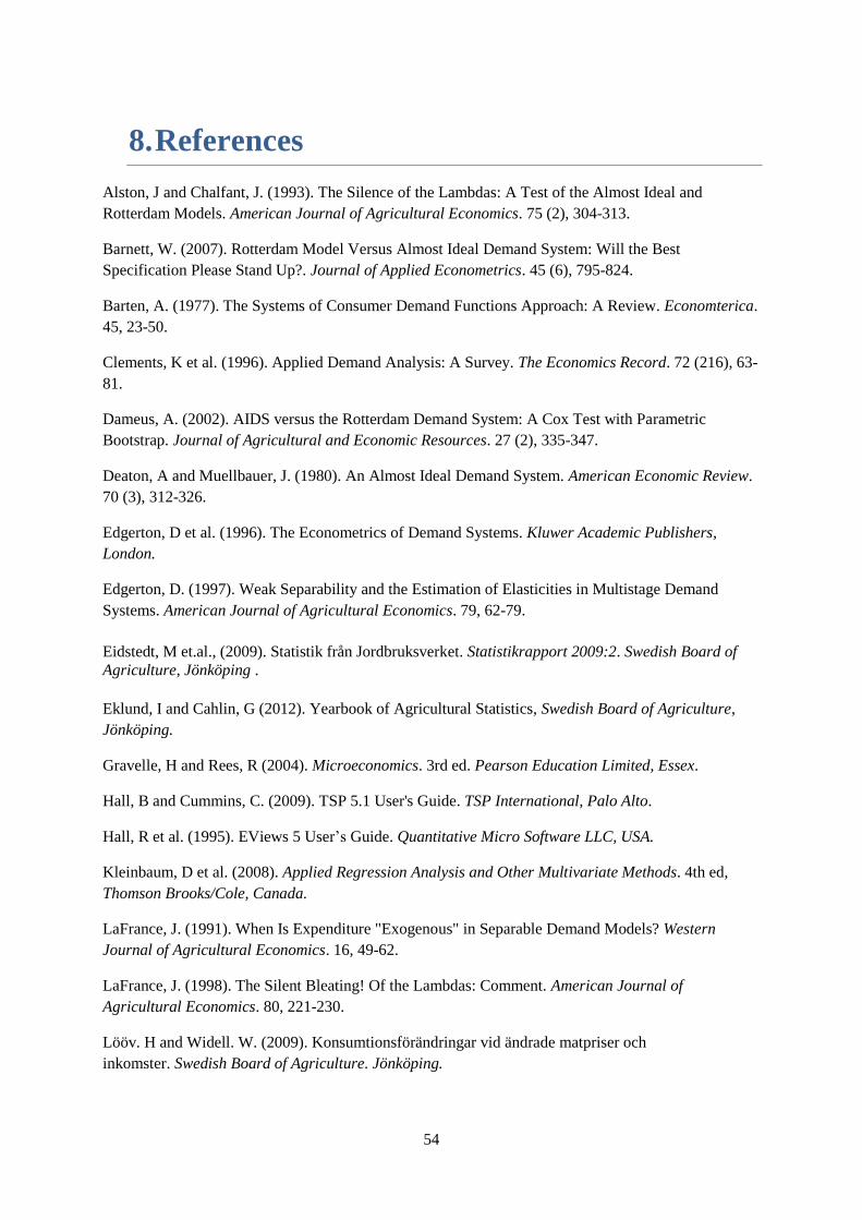
54

8. References

Alston, J and Chalfant, J. (1993). The Silence of the Lambdas: A Test of the Almost Ideal and

Rotterdam Models. American Journal of Agricultural Economics. 75 (2), 304-313.

Barnett, W. (2007). Rotterdam Model Versus Almost Ideal Demand System: Will the Best

Specification Please Stand Up?. Journal of Applied Econometrics. 45 (6), 795-824.

Barten, A. (1977). The Systems of Consumer Demand Functions Approach: A Review. Economterica.

45, 23-50.

Clements, K et al. (1996). Applied Demand Analysis: A Survey. The Economics Record. 72 (216), 63-

81.

Dameus, A. (2002). AIDS versus the Rotterdam Demand System: A Cox Test with Parametric

Bootstrap. Journal of Agricultural and Economic Resources. 27 (2), 335-347.

Deaton, A and Muellbauer, J. (1980). An Almost Ideal Demand System. American Economic Review.

70 (3), 312-326.

Edgerton, D et al. (1996). The Econometrics of Demand Systems. Kluwer Academic Publishers,

London.

Edgerton, D. (1997). Weak Separability and the Estimation of Elasticities in Multistage Demand

Systems. American Journal of Agricultural Economics. 79, 62-79.

Eidstedt, M et.al., (2009). Statistik från Jordbruksverket. Statistikrapport 2009:2. Swedish Board of

Agriculture, Jönköping .

Eklund, I and Cahlin, G (2012). Yearbook of Agricultural Statistics, Swedish Board of Agriculture,

Jönköping.

Gravelle, H and Rees, R (2004). Microeconomics. 3rd ed. Pearson Education Limited, Essex.

Hall, B and Cummins, C. (2009). TSP 5.1 User's Guide. TSP International, Palo Alto.

Hall, R et al. (1995). EViews 5 User’s Guide. Quantitative Micro Software LLC, USA.

Kleinbaum, D et al. (2008). Applied Regression Analysis and Other Multivariate Methods. 4th ed,

Thomson Brooks/Cole, Canada.

LaFrance, J. (1991). When Is Expenditure "Exogenous" in Separable Demand Models? Western

Journal of Agricultural Economics. 16, 49-62.

LaFrance, J. (1998). The Silent Bleating! Of the Lambdas: Comment. American Journal of

Agricultural Economics. 80, 221-230.

Lööv. H and Widell. W. (2009). Konsumtionsförändringar vid ändrade matpriser och

inkomster. Swedish Board of Agriculture. Jönköping.

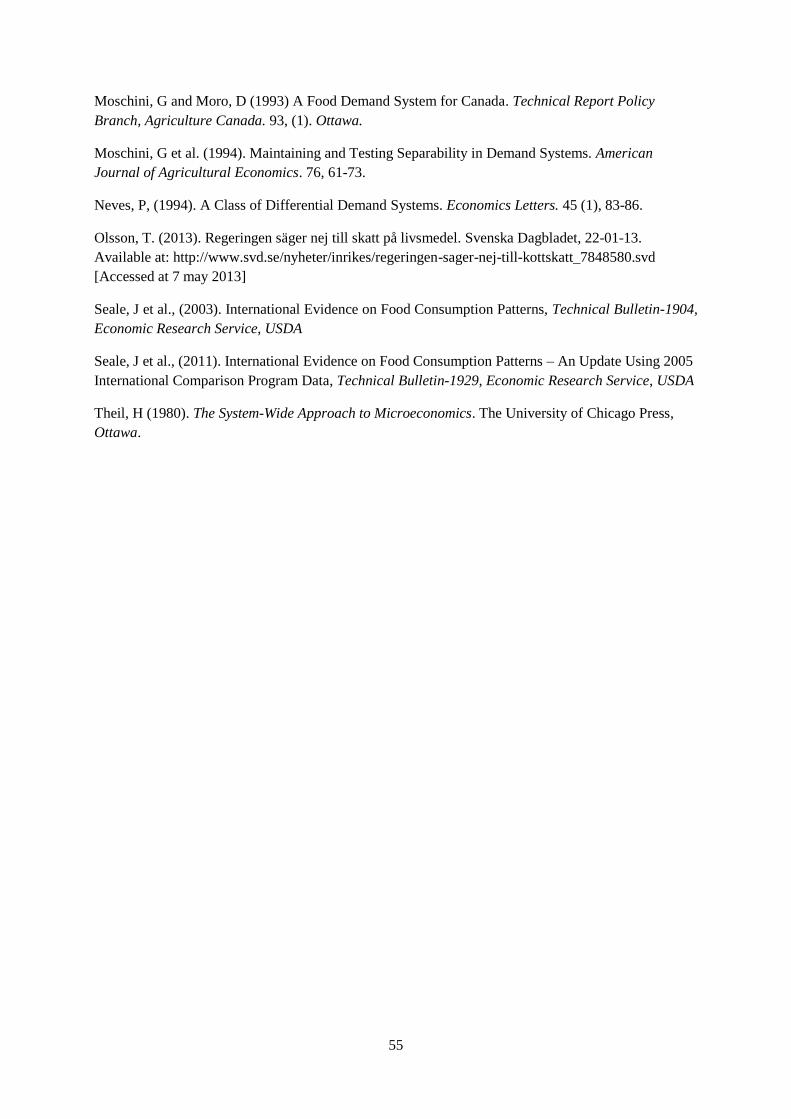
55

Moschini, G and Moro, D (1993) A Food Demand System for Canada. Technical Report Policy

Branch, Agriculture Canada. 93, (1). Ottawa.

Moschini, G et al. (1994). Maintaining and Testing Separability in Demand Systems. American

Journal of Agricultural Economics. 76, 61-73.

Neves, P, (1994). A Class of Differential Demand Systems. Economics Letters. 45 (1), 83-86.

Olsson, T. (2013). Regeringen säger nej till skatt på livsmedel. Svenska Dagbladet, 22-01-13.

Available at: http://www.svd.se/nyheter/inrikes/regeringen-sager-nej-till-kottskatt_7848580.svd

[Accessed at 7 may 2013]

Seale, J et al., (2003). International Evidence on Food Consumption Patterns, Technical Bulletin-1904,

Economic Research Service, USDA

Seale, J et al., (2011). International Evidence on Food Consumption Patterns – An Update Using 2005

International Comparison Program Data, Technical Bulletin-1929, Economic Research Service, USDA

Theil, H (1980). The System-Wide Approach to Microeconomics. The University of Chicago Press,

Ottawa.

56

9. Appendices

Appendix A

The AIDS model

The AIDS model is given in Deaton and Muellbauer (1980):

∑ {

} (2.1.1)

where

and is a parameter and captures changes in relative prices, is total

expenditure and is prices, is commodity budget share. The budget share is therefore a function

of the prices and the total expenditure.

refers to a price index of the following form:

∑

∑∑

Test statistics Durbin-Watson, (Hall and Cummins 2009).

∑

(4.1.1)

Where T is the number of observations, is the sum of the squared residuals.

Lagrange-Multiplier Test, (Hall and Cummins 2009).

(4.1.2)

The LM test follows a chi-square distribution with one degree of freedom.

Jarque-Bera, (Hall et al. 1995).

(4.1.3)

57

Where the number of observation is, is the number of parameters in the regression, is the

skewness of the residuals and is the kurtosis. The JB test statistic is asymptotically chi-square

distributed with two degrees of freedom.

Rotterdam Framework Formulas

The following formulas are used to compute the elasticities within the Rotterdam framework by the

estimated parameters.

Conditional expenditure elasticity:

(4.1.4)

where is the sample mean budget share, and is the estimated marginal budget share.

Hicksian conditional price elasticity:

(4.1.5)

where is the estimated Slutsky parameter.

Marshallian conditional price elasticity:

(4.1.6)

58

Appendix B

Real Expenditure Index

Figure 5.1. Real Per Capita Expenditure Index

Figure 5.1. Real Per Capita Expenditure Index

Figure 5.2. Real Per Capita Expenditure Index

0

20

40

60

80

100

120

140

160

198

0

198

3

198

6

198

9

199

2

199

5

199

8

200

1

200

4

200

7

201

0

Ind

ex V

alue

Year

Expenditure Index, 1980 = 100

Bread and Cereal

Products

Meat

Fish

0

20

40

60

80

100

120

140

Ind

ex V

alue

Year

Expenditure Index, 1980 =100

Milk, Cheese and

Eggs

Oil and Fats

Fruit and

Vegetables

Sweets and Ice

Cream

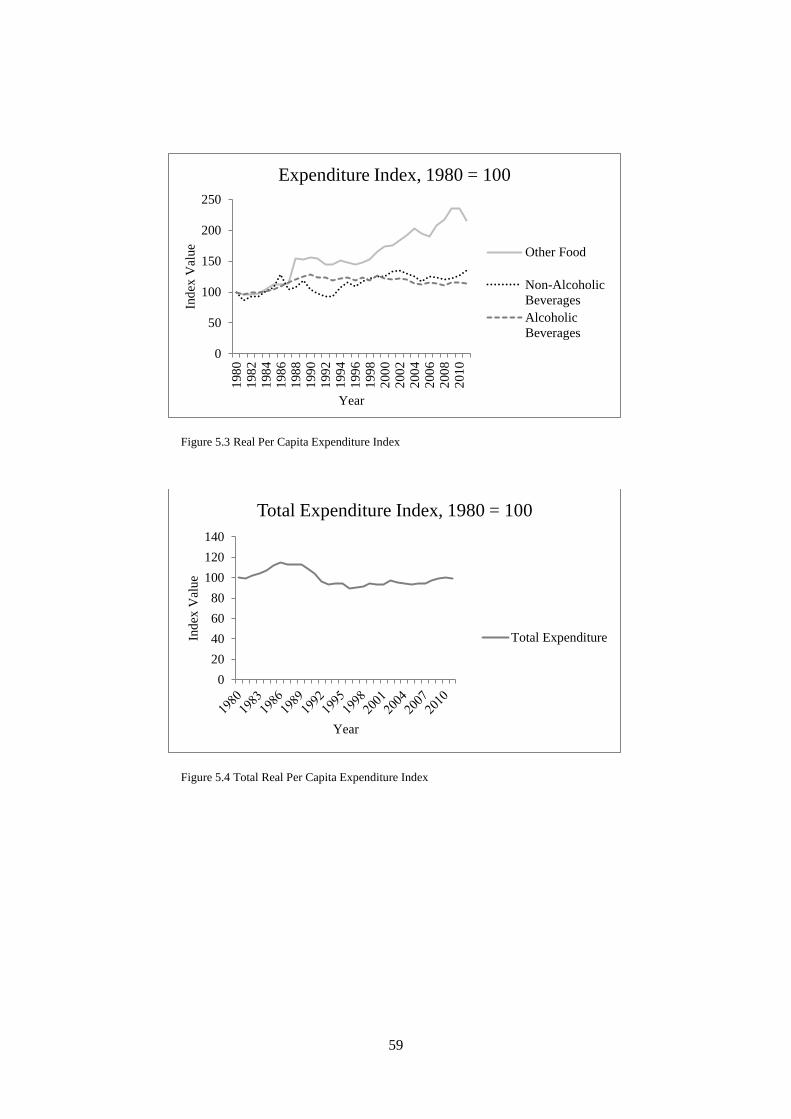
59

Figure 5.3 Real Per Capita Expenditure Index

Figure 5.4 Total Real Per Capita Expenditure Index

0

50

100

150

200

250

198

01

98

21

98

41

98

61

98

81

99

01

99

21

99

41

99

61

99

82

00

02

00

22

00

42

00

62

00

82

01

0

Ind

ex V

alue

Year

Expenditure Index, 1980 = 100

Other Food

Non-Alcoholic

Beverages

Alcoholic

Beverages

0

20

40

60

80

100

120

140

Ind

ex V

alue

Year

Total Expenditure Index, 1980 = 100

Total Expenditure

60

Consumption Per Capita Index

Figure 5.5. Per Capita Consumption Index, Change in Quantity Consumed

Figure 5.6. Per Capita Consumption Index, Change in Quantity Consumed

0

20

40

60

80

100

120

140

160

198

0

198

3

198

6

198

9

199

2

199

5

199

8

200

1

200

4

200

7

201

0

Ind

ex V

alue

Year

Per Capita Consumption Index

Bread and Cereal

Products

Meat

Fish

0

20

40

60

80

100

120

140

Ind

ex V

alue

Year

Per Capita Consumption Index

Milk, Cheese and

Egg

Oil and Fat

Fruit and

Vegeables

Sweets and Ice

Cream

61

Figure 5.7 Per Capita Consumption Index, Change in Quantity Consumed

Conditional Budget Shares

Figure 5.8. Conditional Budget Shares

0

50

100

150

200

250

300

Ind

ex V

alue

Year

Per Capita Consumption Index

Other Foodstuff

Non-Alcoholic

Beverages

Alcoholic

Beverages

0

2

4

6

8

10

12

14

Pre

centa

ge

Years

Budget Shares

Bread and Cereal

Products

Meat

Fish

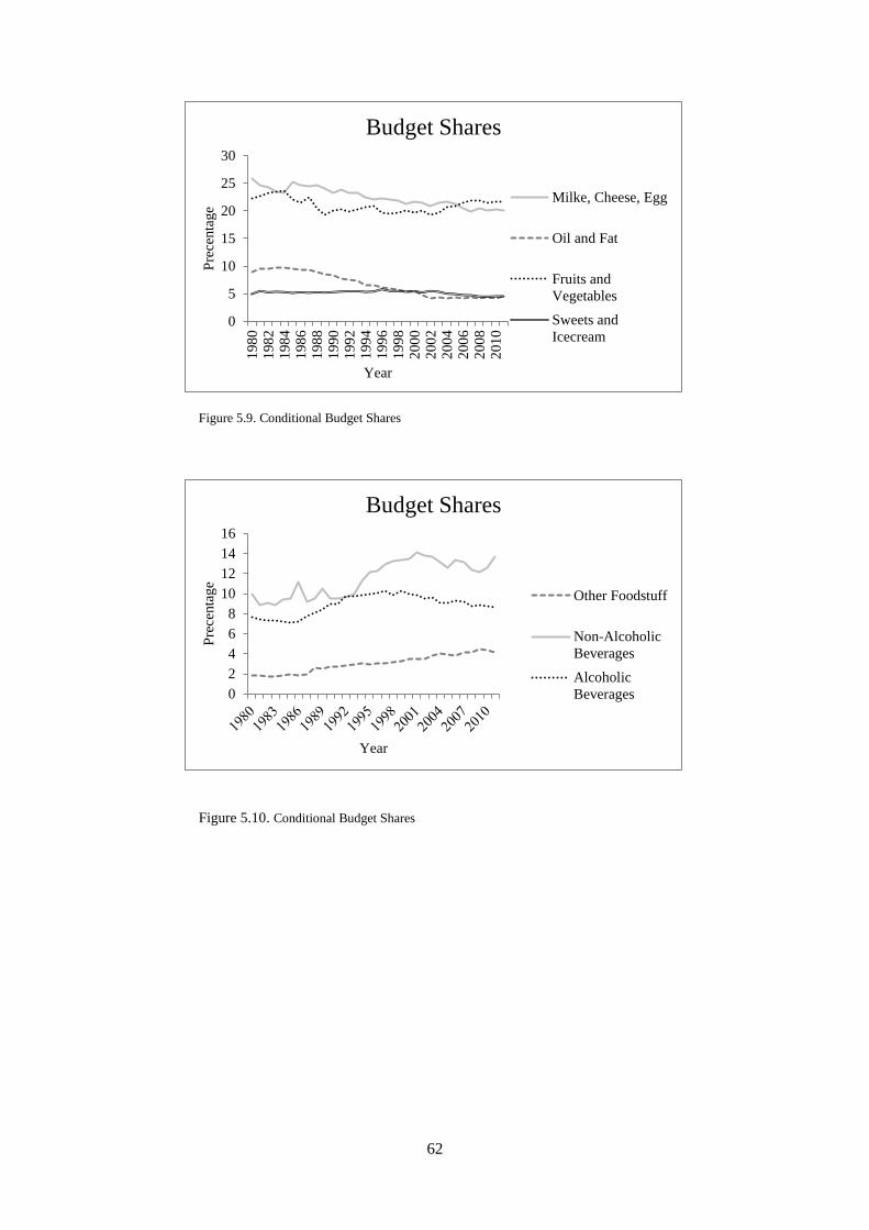
62

Figure 5.9. Conditional Budget Shares

Figure 5.10. Conditional Budget Shares

0

5

10

15

20

25

30

198

01

98

21

98

41

98

61

98

81

99

01

99

21

99

41

99

61

99

82

00

02

00

22

00

42

00

62

00

82

01

0

Pre

centa

ge

Year

Budget Shares

Milke, Cheese, Egg

Oil and Fat

Fruits and

Vegetables

Sweets and

Icecream

0

2

4

6

8

10

12

14

16

Pre

centa

ge

Year

Budget Shares

Other Foodstuff

Non-Alcoholic

Beverages

Alcoholic

Beverages

63

Appendix C

Test Results

4 Obtained from the restriction ∑

Table 6.1.1 Durbin-Watson Test

Test Value

Equation 1 2.2871

Equation 2 1.8269

Equation 3 2.1608

Equation 4 2.1961

Equation 5 1.7933

Equation 6 2.2923

Equation 7 2.0471

Equation 8 2.0730

Table 6.1.2 LM-Test

P-values

Equation 1 0.002

Equation 2 0.130

Equation 3 0.000

Equation 4 0.911

Equation 5 0.202

Equation 6 0.336

Equation 7 0.337

Equation 8 0.089

Table 6.1.3 Jarque-Bera

-values

Equation 1 0.7155

Equation 2 1.2060

Equation 3 1.0830

Equation 4 6.9835

Equation 5 4.3662

Equation 6 0.9743

Equation 7 3.4984

Equation 8 8.5686

Table 6.1.4 Intercept Estimates

Intercept Value

Equation 1 0.0033

Equation 2 0.0052**

Equation 3 -0.0366***

Equation 4 -0.0056

Equation 5 0.0114

Equation 6 -0.0042*

Equation 7 0.0062**

Equation 8 0.0179**

Equation 9 0.00244

Significance level, 10%=*, 5%=** ,1%=***

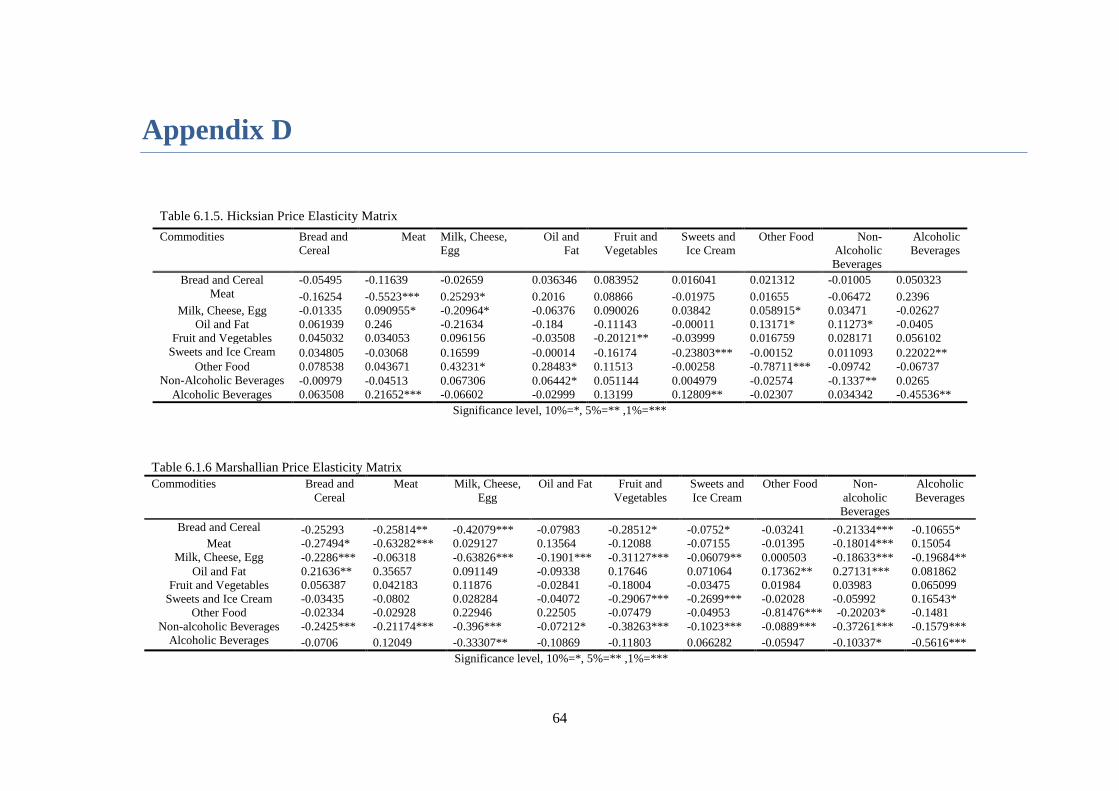
64

Appendix D

Table 6.1.5. Hicksian Price Elasticity Matrix

Commodities Bread and

Cereal

Meat Milk, Cheese,

Egg

Oil and

Fat

Fruit and

Vegetables

Sweets and

Ice Cream

Other Food Non-

Alcoholic

Beverages

Alcoholic

Beverages

Bread and Cereal -0.05495 -0.11639 -0.02659 0.036346 0.083952 0.016041 0.021312 -0.01005 0.050323

Meat -0.16254 -0.5523*** 0.25293* 0.2016 0.08866 -0.01975 0.01655 -0.06472 0.2396

Milk, Cheese, Egg -0.01335 0.090955* -0.20964* -0.06376 0.090026 0.03842 0.058915* 0.03471 -0.02627

Oil and Fat 0.061939 0.246 -0.21634 -0.184 -0.11143 -0.00011 0.13171* 0.11273* -0.0405

Fruit and Vegetables 0.045032 0.034053 0.096156 -0.03508 -0.20121** -0.03999 0.016759 0.028171 0.056102

Sweets and Ice Cream 0.034805 -0.03068 0.16599 -0.00014 -0.16174 -0.23803*** -0.00152 0.011093 0.22022**

Other Food 0.078538 0.043671 0.43231* 0.28483* 0.11513 -0.00258 -0.78711*** -0.09742 -0.06737

Non-Alcoholic Beverages -0.00979 -0.04513 0.067306 0.06442* 0.051144 0.004979 -0.02574 -0.1337** 0.0265

Alcoholic Beverages 0.063508 0.21652*** -0.06602 -0.02999 0.13199 0.12809** -0.02307 0.034342 -0.45536**

Significance level, 10%=*, 5%=** ,1%=***

Table 6.1.6 Marshallian Price Elasticity Matrix Commodities Bread and

Cereal

Meat Milk, Cheese,

Egg

Oil and Fat Fruit and

Vegetables

Sweets and

Ice Cream

Other Food Non-

alcoholic

Beverages

Alcoholic

Beverages

Bread and Cereal -0.25293 -0.25814** -0.42079*** -0.07983 -0.28512* -0.0752* -0.03241 -0.21334*** -0.10655*

Meat -0.27494* -0.63282*** 0.029127 0.13564 -0.12088 -0.07155 -0.01395 -0.18014*** 0.15054

Milk, Cheese, Egg -0.2286*** -0.06318 -0.63826*** -0.1901*** -0.31127*** -0.06079** 0.000503 -0.18633*** -0.19684**

Oil and Fat 0.21636** 0.35657 0.091149 -0.09338 0.17646 0.071064 0.17362** 0.27131*** 0.081862

Fruit and Vegetables 0.056387 0.042183 0.11876 -0.02841 -0.18004 -0.03475 0.01984 0.03983 0.065099

Sweets and Ice Cream -0.03435 -0.0802 0.028284 -0.04072 -0.29067*** -0.2699*** -0.02028 -0.05992 0.16543*

Other Food -0.02334 -0.02928 0.22946 0.22505 -0.07479 -0.04953 -0.81476*** -0.20203* -0.1481

Non-alcoholic Beverages -0.2425*** -0.21174*** -0.396*** -0.07212* -0.38263*** -0.1023*** -0.0889*** -0.37261*** -0.1579***

Alcoholic Beverages -0.0706 0.12049 -0.33307** -0.10869 -0.11803 0.066282 -0.05947 -0.10337* -0.5616***

Significance level, 10%=*, 5%=** ,1%=***

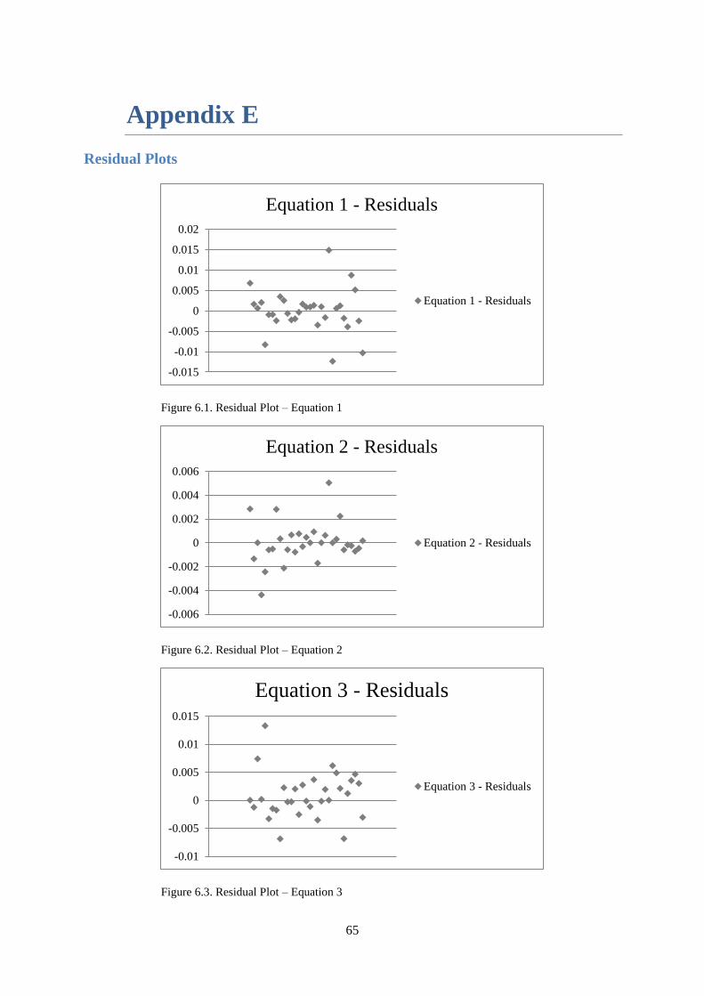
65

Appendix E

Residual Plots

Figure 6.1. Residual Plot – Equation 1

Figure 6.2. Residual Plot – Equation 2

Figure 6.3. Residual Plot – Equation 3

-0.015

-0.01

-0.005

0

0.005

0.01

0.015

0.02

Equation 1 - Residuals

Equation 1 - Residuals

-0.006

-0.004

-0.002

0

0.002

0.004

0.006

Equation 2 - Residuals

Equation 2 - Residuals

-0.01

-0.005

0

0.005

0.01

0.015

Equation 3 - Residuals

Equation 3 - Residuals

66

-0.006

-0.004

-0.002

0

0.002

0.004

0.006

0.008

Equation 4 - Residuals

Equation 4 - Residuals

Figure 6.4. Residual Plot – Equation 4

Figure 6.5. Residual Plot – Equation 5

Figure 6.6. Residual Plot – Equation 6

-0.015

-0.01

-0.005

0

0.005

0.01

0.015

Equation 5 - Residuals

Equation 5 - Residuals

-0.004

-0.002

0

0.002

0.004

0.006

Residuals - Equation 6

Residuals - Equation 6

67

Figure 6.7. Residual Plot – Equation 7

Figure 6.8. Residual Plot – Equation 8

-0.004

-0.002

0

0.002

0.004

0.006

0.008

Residuals - Equation 7

Residuals - Equation 7

-0.01

-0.005

0

0.005

0.01

0.015

Residuals - Equation 8

Residuals - Equation 8

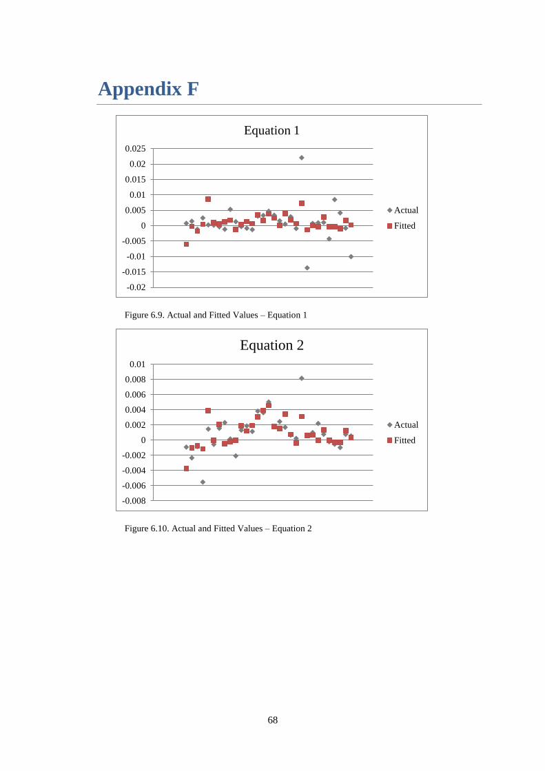
68

Appendix F

Figure 6.9. Actual and Fitted Values – Equation 1

Figure 6.10. Actual and Fitted Values – Equation 2

-0.02

-0.015

-0.01

-0.005

0

0.005

0.01

0.015

0.02

0.025

Equation 1

Actual

Fitted

-0.008

-0.006

-0.004

-0.002

0

0.002

0.004

0.006

0.008

0.01

Equation 2

Actual

Fitted

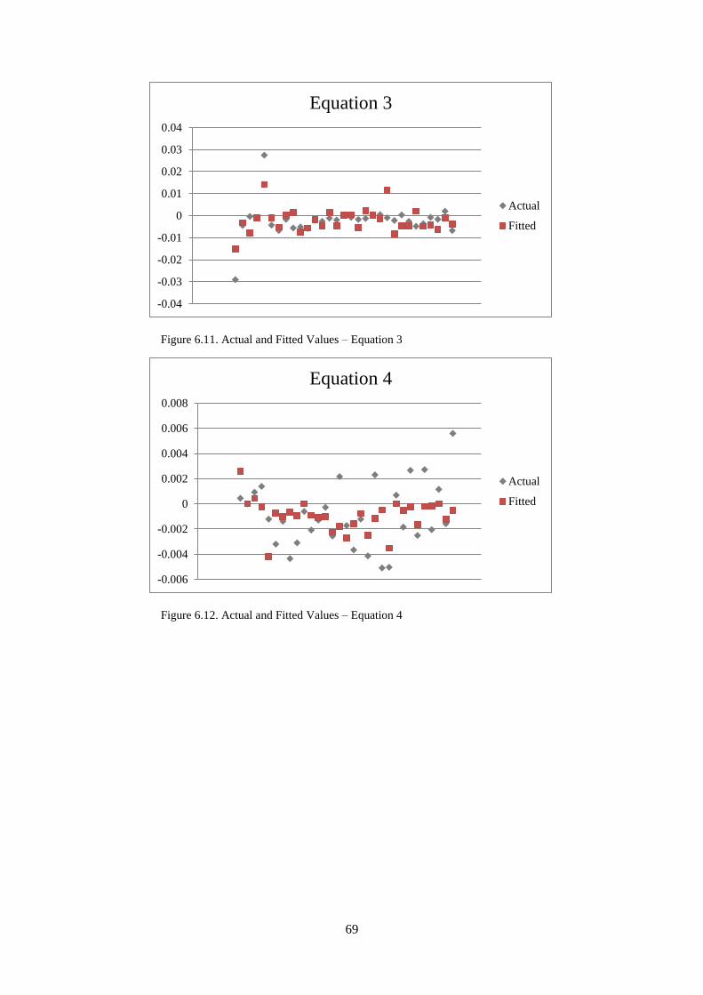
69

Figure 6.11. Actual and Fitted Values – Equation 3

Figure 6.12. Actual and Fitted Values – Equation 4

-0.04

-0.03

-0.02

-0.01

0

0.01

0.02

0.03

0.04

Equation 3

Actual

Fitted

-0.006

-0.004

-0.002

0

0.002

0.004

0.006

0.008

Equation 4

Actual

Fitted

70

Figure 6.13. Actual and Fitted Values – Equation 5

Figure 6.14. Actual and Fitted Values - Equation 6

Figure 6.15. Actual and Fitted Values – Equation 7

-0.015

-0.01

-0.005

0

0.005

0.01

0.015

Equation 5

Actual

Fitted

-0.005

-0.004

-0.003

-0.002

-0.001

0

0.001

0.002

0.003

0.004

0.005

Equation 6

Actual

Fitted

-0.004

-0.002

0

0.002

0.004

0.006

0.008

Equation 7

Actual

Fitted

71

Figure 6.16. Actual and Fitted Values – Equation 8

-0.008

-0.006

-0.004

-0.002

0

0.002

0.004

0.006

0.008

0.01

0.012

0.014

Equation 8

Actual

Fitted