the symmetrization problem for multiple … · 2013-10-28 · pr´e-publicac¸˜oes do departamento...
TRANSCRIPT

Pre-Publicacoes do Departamento de MatematicaUniversidade de CoimbraPreprint Number 13–48
THE SYMMETRIZATION PROBLEM FOR MULTIPLEORTHOGONAL POLYNOMIALS
AMILCAR BRANQUINHO AND EDMUNDO J. HUERTAS
Abstract: We analyze the effect of symmetrization in the theory of multiple or-thogonal polynomials. For a symmetric sequence of type II multiple orthogonalpolynomials satisfying a high–term recurrence relation, we fully characterize theWeyl function associated to the corresponding block Jacobi matrix as well as theStieltjes matrix function. Next, from an arbitrary sequence of type II multiple or-thogonal polynomials with respect to a set of d linear functionals, we obtain a totalof d + 1 sequences of type II multiple orthogonal polynomials, which can be usedto construct a new sequence of symmetric type II multiple orthogonal polynomials.Finally, we prove a Favard-type result for certain sequences of matrix multiple or-thogonal polynomials satisfying a matrix four–term recurrence relation with matrixcoefficients.
Keywords: Matrix orthogonal polynomials, linear functional, recurrence relation,operator theory, matrix Sylvester differential equations, full Kostant-Toda systems.AMS Subject Classification (2000): 33C45, 39B42.
1. Introduction
In recent years an increasing attention has been paid to the notion of mul-tiple orthogonality. Multiple orthogonal polynomials are a generalization oforthogonal polynomials [11], satisfying orthogonality conditions with respectto a number of measures, instead of just one measure. There exists a vastliterature on this subject, e.g. the classical works [1], [2], [18, Ch. 23] and [27]among others. A characterization through a vectorial functional equation,where the authors call them d–orthogonal polynomials instead of multipleorthogonal polynomials, was done in [14]. Their asymptotic behavior havebeen studied in [4], also continued in [12], and properties for their zeros havebeen analyzed in [17].
Received October 28, 2013.The work of the first author was partially supported by Centro de Matematica da Universidade
de Coimbra (CMUC), funded by the European Regional Development Fund through the programCOMPETE and by the Portuguese Government through the FCT - Fundacao para a Ciencia e aTecnologia under the project PEst-C/MAT/UI0324/2011. The work of the second author was sup-ported by Fundacao para a Ciencia e a Tecnologia (FCT) of Portugal, ref. SFRH/BPD/91841/2012,and partially supported by Direccion General de Investigacion Cientıfica y Tecnica, Ministerio deEconomıa y Competitividad of Spain, grant MTM2012-36732-C03-01.
1
2 BRANQUINHO AND HUERTAS
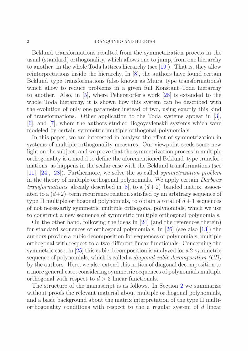
Bcklund transformations resulted from the symmetrization process in theusual (standard) orthogonality, which allows one to jump, from one hierarchyto another, in the whole Toda lattices hierarchy (see [19]). That is, they allowreinterpretations inside the hierarchy. In [8], the authors have found certainBcklund–type transformations (also known as Miura–type transformations)which allow to reduce problems in a given full Konstant–Toda hierarchyto another. Also, in [5], where Peherstorfer’s work [28] is extended to thewhole Toda hierarchy, it is shown how this system can be described withthe evolution of only one parameter instead of two, using exactly this kindof transformations. Other application to the Toda systems appear in [3],[6], and [7], where the authors studied Bogoyavlenskii systems which weremodeled by certain symmetric multiple orthogonal polynomials.In this paper, we are interested in analyze the effect of symmetrization in
systems of multiple orthogonality measures. Our viewpoint seeds some newlight on the subject, and we prove that the symmetrization process in multipleorthogonality is a model to define the aforementioned Bcklund–type transfor-mations, as happens in the scalar case with the Bcklund transformations (see[11], [24], [28]). Furthermore, we solve the so called symmetrization problemin the theory of multiple orthogonal polynomials. We apply certain Darbouxtransformations, already described in [8], to a (d+2)–banded matrix, associ-ated to a (d+2)–term recurrence relation satisfied by an arbitrary sequence oftype II multiple orthogonal polynomials, to obtain a total of d+1 sequencesof not necessarily symmetric multiple orthogonal polynomials, which we useto construct a new sequence of symmetric multiple orthogonal polynomials.On the other hand, following the ideas in [24] (and the references therein)
for standard sequences of orthogonal polynomials, in [26] (see also [13]) theauthors provide a cubic decomposition for sequences of polynomials, multipleorthogonal with respect to a two different linear functionals. Concerning thesymmetric case, in [25] this cubic decomposition is analyzed for a 2-symmetricsequence of polynomials, which is called a diagonal cubic decomposition (CD)by the authors. Here, we also extend this notion of diagonal decomposition toa more general case, considering symmetric sequences of polynomials multipleorthogonal with respect to d > 3 linear functionals.The structure of the manuscript is as follows. In Section 2 we summarize
without proofs the relevant material about multiple orthogonal polynomials,and a basic background about the matrix interpretation of the type II multi-orthogonality conditions with respect to the a regular system of d linear

SYMMETRIZATION PROBLEM IN MULTIPLE ORTHOGONALITY 3
functionals u1, . . . , ud and diagonal multi–indices. In Section 3 we fullycharacterize the Weyl function RJ and the Stieltjes matrix function F associ-ated to the block Jacobi matrix J corresponding to a (d+2)–term recurrencerelation satisfied by a symmetric sequence of type II multiple orthogonal po-lynomials. In Section 4, starting from an arbitrary sequence of type II mul-tiple polynomials satisfying a (d+ 2)–term recurrence relation, we state theconditions to find a total of d+1 sequences of type II multiple orthogonal po-lynomials, in general non–symmetric, which can be used to construct a newsequence of symmetric type II multiple orthogonal polynomials. Moreover,we also deal with the converse problem, i.e., we propose a decomposition ofa given symmetric type II multiple orthogonal polynomial sequence, whichallows us to find a set of other (in general non–symmetric) d + 1 sequencesof type II multiple orthogonal polynomials, satisfying in turn (d + 2)–termrecurrence relations. Finally, in Section 5, we present a Favard-type result,showing that certain 3 × 3 matrix decomposition of a type II multiple 2–orthogonal polynomials, satisfy a matrix four–term recurrence relation, andtherefore it is type II multiple 2–orthogonal (in a matrix sense) with respectto a certain system of matrix measures.
2. Definitions and matrix interpretation of multiple or-
thogonality
Let n = (n1, ..., nd) ∈ Nd be a multi–index with length |n| := n1 + · · ·+ nd
and let ujdj=1 be a set of linear functionals, i.e. uj : P → C. Let Pn be asequence of polynomials, with degPn is at most |n|. Pn is said to be type IImultiple orthogonal with respect to the set of linear functionals uj
dj=1 and
multi–index n if
uj(xkPn) = 0 , k = 0, 1, . . . , nj − 1 , j = 1, . . . , d . (1)
A multi–index n is said to be normal for the set of linear functionals ujdj=1,
if the degree of Pn is exactly |n| = n. When all the multi–indices of a givenfamily are normal, we say that the set of linear functionals uj
dj=1 is regular.
In the present work, we will restrict our attention ourselves to the so calleddiagonal multi–indices n = (n1, ..., nd) ∈ I, where
I = (0, 0, . . . , 0), (1, 0, . . . , 0), . . . , (1, 1, . . . , 1),
(2, 1, . . . , 1), . . . , (2, 2, . . . , 2), . . ..

4 BRANQUINHO AND HUERTAS
Notice that there exists a one to one correspondence, i, between the above setof diagonal multi–indices I ⊂ N
d and N, given by i(Nd) = |n| = n. Therefore,to simplify the notation, we write in the sequel Pn ≡ P|n| = Pn. The left–multiplication of a linear functional u : P → C by a polynomial p ∈ P isgiven by the new linear functional p u : P → C such that
p u(xk) = u(p(x)xk) , k ∈ N .
Next, we briefly review a matrix interpretation of type II multiple orthogo-nal polynomials with respect to a system of d regular linear functionals anda family of diagonal multi–indices. Throughout this work, we will use thismatrix interpretation as a useful tool to obtain some of the main results ofthe manuscript. For a recent and deeper account of the theory (in a moregeneral framework, considering quasi–diagonal multi–indices) we refer thereader to [10].Let us consider the family of vector polynomials
Pd =
[P1 · · · Pd
]T, d ∈ N, Pj ∈ P,
and Md×d the set of d× d matrices with entries in C. Let Xj be the familyof vector polynomials Xj ∈ P
d defined by
Xj =[xjd · · · x(j+1)d−1
]T, j ∈ N, (2)
where X0 =[1 · · · xd−1
]T. By means of the shift n → nd, associated with
Pn, we define the sequence of vector polynomials Pn, with
Pn =[Pnd(x) · · · P(n+1)d−1(x)
]T, n ∈ N, Pn ∈ P
d. (3)
Let uj : P → C with j = 1, . . . , d a system of linear functionals as in (1).
From now on, we define the vector of functionals U =[u1 · · · ud
]Tacting
in Pd → Md×d, by
U(P) =(U·PT
)T=
u1(P1) · · · ud(P1)
... . . . ...u1(Pd) · · · ud(Pd)
.
Let
Aℓ(x) =ℓ∑
k=0
Aℓk x
k,
be a matrix polynomial of degree ℓ, where Aℓk ∈ M2×2, and U a vector of
functional. We define the new vector of functionals called left multiplication
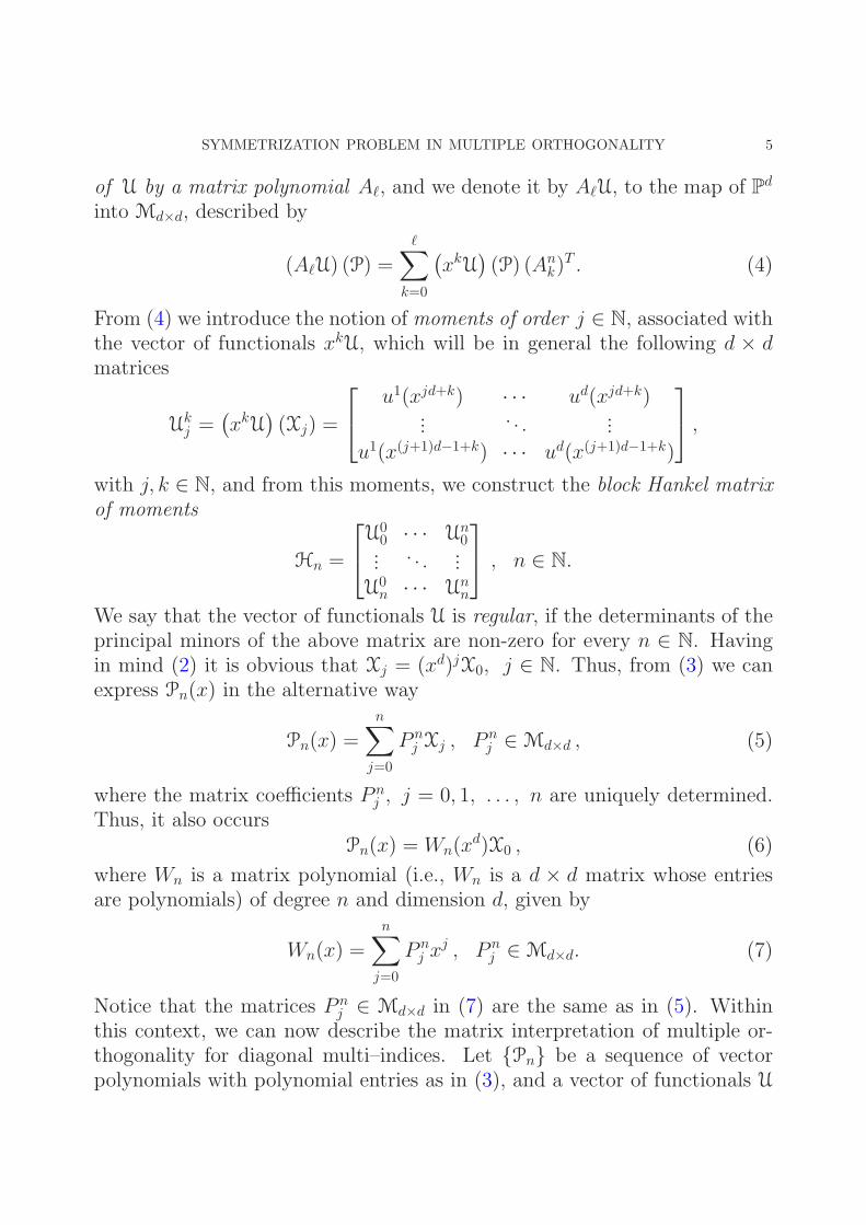
SYMMETRIZATION PROBLEM IN MULTIPLE ORTHOGONALITY 5
of U by a matrix polynomial Aℓ, and we denote it by AℓU, to the map of Pd
into Md×d, described by
(AℓU) (P) =ℓ∑
k=0
(xkU
)(P) (An
k)T . (4)
From (4) we introduce the notion of moments of order j ∈ N, associated withthe vector of functionals xkU, which will be in general the following d × dmatrices
Ukj =
(xkU
)(Xj) =
u1(xjd+k) · · · ud(xjd+k)... . . . ...
u1(x(j+1)d−1+k) · · · ud(x(j+1)d−1+k)
,
with j, k ∈ N, and from this moments, we construct the block Hankel matrixof moments
Hn =
U0
0 · · · Un0
... . . . ...U0
n · · · Unn
, n ∈ N.
We say that the vector of functionals U is regular, if the determinants of theprincipal minors of the above matrix are non-zero for every n ∈ N. Havingin mind (2) it is obvious that Xj = (xd)jX0, j ∈ N. Thus, from (3) we canexpress Pn(x) in the alternative way
Pn(x) =n∑
j=0
P nj Xj , P n
j ∈ Md×d , (5)
where the matrix coefficients P nj , j = 0, 1, . . . , n are uniquely determined.
Thus, it also occursPn(x) = Wn(x
d)X0 , (6)
where Wn is a matrix polynomial (i.e., Wn is a d × d matrix whose entriesare polynomials) of degree n and dimension d, given by
Wn(x) =n∑
j=0
P nj x
j , P nj ∈ Md×d. (7)
Notice that the matrices P nj ∈ Md×d in (7) are the same as in (5). Within
this context, we can now describe the matrix interpretation of multiple or-thogonality for diagonal multi–indices. Let Pn be a sequence of vectorpolynomials with polynomial entries as in (3), and a vector of functionals U

6 BRANQUINHO AND HUERTAS
as described above. Pn is said to be a type II vector multiple orthogonalpolynomial sequence with respect to the vector of functionals U, and a set ofdiagonal multi–indices, if
i) (xkU)(Pn) = 0d×d , k = 0, 1, . . . , n− 1 ,ii) (xnU)(Pn) = ∆n ,
(8)
where ∆n is a regular upper triangular d× d matrix (see [10, Th. 3] consid-ering diagonal multi–indices).Next, we introduce a few aspects of the duality theory, which will be useful
in the sequel. We denote by P∗ the dual space of P, i.e. the linear space
of linear functionals defined on P over C. Let Pn be a sequence of monicpolynomials. We call ℓn, ℓn ∈ P
∗, the dual sequence of Pn if ℓi(Pj) =δi,j, i, j ∈ N holds. Given a sequence of linear functionals ℓn ∈ P
∗, bymeans of the shift n → nd, the vector sequence of linear functionals Ln,with
Ln =[ℓnd · · · ℓ(n+1)d−1
]T, n ∈ N, (9)
is said to be the vector sequence of linear functionals associated with ℓn.It is very well known (see [14]) that a given sequence of type II polynomials
Pn, simultaneously orthogonal with respect to a d linear functionals, orsimply d–orthogonal polynomials, satisfy the following (d + 2)–term orderrecurrence relation
xPn+d(x) = Pn+d+1(x) + βn+dPn+d(x) +d−1∑
ν=0
γd−1−νn+d−νPn+d−1−ν(x) , (10)
γ0n+1 6= 0 for n ≥ 0, with the initial conditions P0(x) = 1, P1(x) = x − β0,
and
Pn(x) = (x− βn−1)Pn−1(x)−n−2∑
ν=0
γd−1−νn−1−νPn−2−ν(x) , 2 ≤ n ≤ d .
E.g., if d = 2, the sequence of monic type II multiple orthogonal polynomialsPn with respect to the regular system of functionals u1, u2 and normalmulti–index satisfy, for every n ≥ 0, the following four term recurrence rela-tion (see [10, Lemma 1-a], [22])
xPn+2(x) = Pn+3(x) + βn+2Pn+2(x) + γ1n+2Pn+1(x) + γ0
n+1Pn(x) , (11)
where βn+2, γ1n+2, γ
0n+1 ∈ C, γ0
n+1 6= 0, P0(x) = 1, P1(x) = x−β0 and P2(x) =(x− β1)P1(x)− γ1
1P0(x).

SYMMETRIZATION PROBLEM IN MULTIPLE ORTHOGONALITY 7
We follow [14, Def. 4.1.] in assuming that a monic system of polynomialsSn is said to be d–symmetric when it verifies
Sn(ξkx) = ξnkSn(x) , n ≥ 0 , (12)
where ξk = exp (2kπi/(d+ 1)), k = 1, . . . , d, and ξd+1k = 1. Notice that,
if d = 1, then ξk = −1 and therefore Sn(−x) = (−1)nSn(x) (see [11]).We also assume (see [14, Def. 4.2.]) that the vector of linear functionals
L0 =[ℓ0 · · · ℓd−1
]Tis said to be d–symmetric when the moments of its
entries satisfy, for every n ≥ 0,
ℓν(x(d+1)n+µ) = 0 , ν = 0, 1, . . . , d− 1 , µ = 0, 1, . . . , d , ν 6= µ . (13)
Observe that if d = 1, this condition leads to the well known fact ℓ0(x2n+1) =
0, i.e., all the odd moments of a symmetric moment functional are zero(see [11, Def. 4.1, p.20]).Under the above assumptions, we have the following
Theorem 1 (cf. [14, Th. 4.1]). For every sequence of monic polynomialsSn, d–orthogonal with respect to the vector of linear functionals L0 =[ℓ0 · · · ℓd−1
]T, the following statements are equivalent:
(a) The vector of linear functionals L0 is d–symmetric.(b) The sequence Sn is d–symmetric.(c) The sequence Sn satisfies
xSn+d(x) = Sn+d+1(x) + γn+1Sn(x) , n ≥ 0, (14)
with Sn(x) = xn for 0 ≤ n ≤ d.
Notice that (14) is a particular case of the (d+2)–term recurrence relation(10). Continuing the same trivial example above for d = 2, it directly impliesthat the sequence of polynomials Sn, satisfy the particular case of (10), i.e.S0(x) = 1, S1(x) = 1, S2(x) = x2 and
xSn+2(x) = Sn+3(x) + γn+1Sn(x) , n ≥ 0.
Notice that the coefficients βn+2 and γ1n+2 of polynomials Sn+2 and Sn+1
respectively, on the right hand side of (11) are zero.On the other hand, the (d+2)–term recurrence relation (14) can be rewrit-
ten in terms of vector polynomials (3), and then we obtain what will bereferred to as the symmetric type II vector multiple orthogonal polynomial

8 BRANQUINHO AND HUERTAS
sequence Sn =[Snd · · · S(n+1)d−1
]T. For n → dn+ j, j = 0, 1, . . . d− 1 and
n ∈ N, we have the following matrix three term recurrence relation
xSn = ASn+1 +BSn + CnSn−1 , n = 0, 1, . . . (15)
with S−1 =[0 · · · 0
]T, S0 =
[S0 · · · Sd−1
]T, and matrix coefficients A,
B, Cn ∈ Md×d given
A =
0 0 · · · 0...
... . . . ...0 0 · · · 01 0 · · · 0
, B =
0 1. . . . . .
0 10
, and (16)
Cn = diag [γ1, γ2, . . . , γnd].
Note that, in this case, one has
S0 = X0 =[1 x · · · xd−1
]T.
Since Sn satisfies (14), it is clear that this d–symmetric type II multiplepolynomial sequence will be orthogonal with respect to certain system of dlinear functionals, say v1, . . . , vd. Hence, according to the matrix interpre-tation of multiple orthogonality, the corresponding type II vector multiplepolynomial sequence Sn will be orthogonal with respect to a symmetric
vector of functionals V =[v1 · · · vd
]T. The corresponding matrix ortho-
gonality conditions for Sn and V are described in (8).One of the main goals of this manuscript is to analyze symmetric sequences
of type II vector multiple polynomials, orthogonal with respect to a symmet-ric vector of functionals. The remainder of this section will be devoted to theproof of one of our main results concerning the moments of the d functionalentries of such symmetric vector of functionals V. The following theoremstates that, under certain conditions, the moment of each functional entryin V can be given in terms of the moments of other functional entry in thesame V.
Lemma 1. If V =[v1 · · · vd
]Tis a symmetric vector of functionals, the
moments of each functional entry vj, j = 1, 2, . . . , d in V, can be expressedfor all n ≥ 0 as
(i) If µ = 0, 1, . . . , j − 2
vj(x(d+1)n+µ) =vj,µ
vµ+1,µvµ+1(x(d+1)n+µ), (17)

SYMMETRIZATION PROBLEM IN MULTIPLE ORTHOGONALITY 9
where vk,l = vk(Sl).(ii) If µ = j − 1, the value vj(x(d+1)n+µ) depends on vj, and it is different
from zero.(iii) If µ = j, j + 1, . . . , d
vj(x(d+1)n+µ) = 0.
Proof : In the matrix framework of multiple orthogonality, the type II vectorpolynomials Sn are multiple orthogonal with respect to the symmetric vector
moment of functionals V : Pd → Md×d, with V =
[v1 · · · vd
]T. If we
multiply (15) by xn−1, together with the linearity of V, we get, for n = 0, 1, . . .
V (xnSn) = AV(xn−1
Sn+1
)+BV
(xn−1
Sn
)+ CnV
(xn−1
Sn−1
), n = 0, 1, . . . .
By the orthogonality conditions (8) for V, we have
AV(xn−1
Sn+1
)= BV
(xn−1
Sn
)= 0d×d , n = 0, 1, . . . ,
and iterating the remain expression
V (xnSn) = CnV(xn−1
Sn−1
), n = 0, 1, . . .
we obtain
V (xnSn) = CnCn−1 · · ·C1V (S0) , n = 0, 1, . . . .
The above matrix V (S0) is given by
V (S0) = V00 =
v1(S0) · · · vd(S0)... . . . ...
v1(Sd−1) · · · vd(Sd−1)
.
To simplify the notation, in the sequel vi,j−1 denotes vi(Sj−1). Notice that(8) leads to the fact that the above matrix is an upper triangular matrix,which in turn means that vi,j−1 = 0, for every i, j = 1, . . . , d− 1, that is
V00 =
v1,0 v2,0 · · · vd,0v2,1 · · · vd,1
. . . ...vd,d−1
. (18)
Let L0 be a d–symmetric vector of linear functionals as in Theorem 1. Wecan express V in terms of L0 as V = G0L0. Thus, we have
(G−10 V)(S0) = L0(S0) = Id .

10 BRANQUINHO AND HUERTAS
From (4) we have
(G−1
0 V)(S0) = V (S0) (G
−10 )T = V
00(G
−10 )T = Id .
Therefore, taking into account (18), we conclude
G0 = (V00)
T =
v1,0v2,0 v2,1...
... . . .vd,0 vd,1 · · · vd,d−1
. (19)
Observe that the matrix (V00)
T is lower triangular, and every entry in theirmain diagonal is different from zero, so G0 always exists and is a lower tri-angular matrix. Since V = G0L0, we finally obtain the expressions
v1 = v1,0ℓ0,v2 = v2,0ℓ0 + v2,1ℓ1,v3 = v3,0ℓ0 + v3,1ℓ1 + v3,2ℓ2,· · ·vd = vd,0ℓ0 + vd,1ℓ1 + · · ·+ vd,d−1ℓd−1,
(20)
between the entries of L0 and V.Next, from (20), (13), together with the crucial fact that every value in the
main diagonal of V00 is different from zero, it is a simple matter to check that
the three statements of the lemma follow. We conclude the proof only forthe functionals v2 and v1. The other cases can be deduced in a similar way.From (20) we get v1(x(d+1)n+µ) = v1,0 · ℓ0(x
(d+1)n+µ) 6= 0. Then, from (13)we see that for every µ 6= 0 we have v1(x(d+1)n+µ) = 0 (statement (iii)). Ifµ = 0, we have v1(x(d+1)n) = v1,0 ·ℓ0(x
(d+1)n) 6= 0 (statement (ii)). Next, from(20) we get v2(x(d+1)n+µ) = v2,0 ·ℓ0(x
(d+1)n+µ)+v2,1 ·ℓ1(x(d+1)n+µ). Then, from
(13) we see that for every µ 6= 1, we have v2(x(d+1)n+µ) = 0 (statement (iii)).If µ = 0 we have
v2(x(d+1)n) =v2,0v1,0
v1(x(d+1)n) (statement (i)).
If µ = 1 then v2(x(d+1)n+1) = v2,1 · ℓ1(x(d+1)n+1) 6= 0 (statement (ii)).
Thus, the lemma follows.

SYMMETRIZATION PROBLEM IN MULTIPLE ORTHOGONALITY 11
3. Representation of the Stieltjes and Weyl functions
Let U a vector of functionals U =[u1 · · · ud
]T. We define the Stieltjes
matrix function associated to U (or matrix generating function associated toU), F by (see [10])
F(z) =∞∑
n=0
(xnU) (X0(x))
zn+1.
In this Section we find the relation between the Stieltjes matrix functionF, associated to a certain d–symmetric vector of functionals V, and certaininteresting function associated to the corresponding block Jacobi matrix J .Here we deal with d–symmetric sequences of type II multiple orthogonalpolynomials Sn, and hence J is a (d + 2)–banded matrix with only twoextreme non-zero diagonals, which is the block–matrix representation of thethree–term recurrence relation with d×d matrix coefficients, satisfied by thevector sequence of polynomials Sn (associated to Sn), orthogonal withrespect to V.Thus, the shape of a Jacobi matrix J , associated with the (d+2)–term re-
currence relation (14) satisfied by a d–symmetric sequence of type II multipleorthogonal polynomials Sn is
J =
0 10 0 1... . . . . . .0 0 1γ1 0 0 1
γ2 0 0 . . .. . . . . . . . .
. (21)
We can rewrite J as the block tridiagonal matrix
J =
B AC1 B A
C2 B A. . . . . . . . .
associated to a three term recurrence relation with matrix coefficients, satis-fied by the sequence of type II vector multiple orthogonal polynomials Snassociated to Sn. Here, every block matrix A, B and Cn has d × d size,

12 BRANQUINHO AND HUERTAS
and they are given in (16). When J is a bounded operator, it is possible todefine the resolvent operator by
(zI − J)−1 =∞∑
n=0
Jn
zn+1, |z| > ||J ||,
(see [9]) and we can put in correspondence the following block tridiagonalanalytic function, known as the Weyl function associated with J
RJ(z) =∞∑
n=0
eT0 Jn e0
zn+1, |z| > ||J ||, (22)
where e0 =[Id 0d×d · · ·
]T. If we denote by Mij the d× d block matrices of
a semi-infinite matrix M , formed by the entries of rows d(i − 1) + 1, d(i −1) + 2, . . . , di , and columns d(j − 1) + 1, d(j − 1) + 2, . . . , dj , the matrix Jn
can be written as the semi-infinite block matrix
Jn =
Jn11 Jn
12 · · ·Jn21 Jn
22 · · ·...
... . . .
.
We can now formulate our first important result in this Section. For moredetails we refer the reader to [6, Sec. 1.2] and [3].Let Sn be a symmetric type II vector multiple polynomial sequence or-
thogonal with respect to the d–symmetric vector of functionals V. Following[10, Th. 7], the matrix generating function associated to V, and the Weylfunction associated with J , the block Jacobi matrix corresponding to Sn,can be put in correspondence by means of the matrix expression
F(z) = RJ(z)V(X0) , (23)
where, for the d–symmetric case, V(X0) = V(S0) = V00, which is explicitly
given in (18).First we study the case d = 2, and next we consider more general situations
for d > 2 functional entries in V. From Lemma 1, we obtain the entries forthe representation of the Stieltjes matrix function F(z), associated with V =

SYMMETRIZATION PROBLEM IN MULTIPLE ORTHOGONALITY 13
[v1 v2
], as
F(z) =∞∑
n=0
[v1(x3n)
v2,0·v1(x3n)
v1,0
0 v2(x3n+1)
]/z3n+1 +
∞∑
n=0
[0 v2(x3n+1)0 0
]/z3n+2
+∞∑
n=0
[0 0
v1(x3n+3)v2,0·v
1(x3n+3)v1,0
]/z3n+3 . (24)
Notice that we have F(z) = F1(z) + F2(z) + F3(z). The following theoremshows that we can obtain F(z) in our particular case, analyzing two differentsituations.
Theorem 2. Let V =[v1 v2
]Tbe a symmetric vector of functionals, with
d = 2. Then the Weyl function is given by
RJ(z) =∞∑
n=0
[v1(x3n)v1,0
0
0 v2(x3n+1)v2,1
]
z3n+1+
∞∑
n=0
[0 v2(x3n+1)
v2,1
0 0
]
z3n+2+
∞∑
n=0
[0 0
v1(x3n+3)v1,0
0
]
z3n+3
Proof : It is enough to multiply (24) by (V00)
−1. The explicit expression forV00 is given in (18).
Computations considering d > 2 functionals, can be cumbersome butdoable. The matrix generating function F (as well as the Weyl function),will be the sum of d + 1 matrix terms, i.e. F(z) = F1(z) + · · · + Fd+1(z),each of them of size d× d.Let us now outline the very interesting structure of RJ(z) for the general
case of d functionals. We shall describe the structure of RJ(z) for d = 3,comparing the situation with the general case. Let ∗ denote every non-zeroentry in a given matrix. Thus, there will be four J11 matrices of size 3 × 3.
Here, and in the general case, the first matrix [J(d+1)n11 ]d×d will allways be
diagonal, as follows
[J4n11 ]3×3 =
∗ 0 00 ∗ 00 0 ∗
.

14 BRANQUINHO AND HUERTAS
Indeed, observe that for n = 0, [J(d+1)n11 ]d×d = Id. Next, we have
[J4n+111 ]3×3 =
0 ∗ 00 0 ∗0 0 0
.
From (14) we know that the “distance” between the two extreme non-zerodiagonals of J will allways consist of d zero diagonals. It directly implies
that, also in the general case, every entry in the last row of [J(d+1)n11 ]d×d will
always be zero, and therefore the unique non-zero entries in [J(d+1)n11 ]d×d will
be one step over the main diagonal.Next we have
[J4n+211 ]3×3 =
0 0 ∗0 0 0∗ 0 0
.
Notice that for every step, the main diagonal in [J(d+1)n11 ]d×d goes “one diago-
nal” up, but the other extreme diagonal of J is also moving upwards, withexactly d zero diagonals between them. It directly implies that, no matter
the number of functionals, only the lowest-left element of [J(d+1)n+211 ]d×d will
be different from zero. Finally, we have
[J4n+311 ]3×3 =
0 0 0∗ 0 00 ∗ 0
.
Here, the last non-zero entry of the main diagonal in [J4n11 ]3×3 vanishes. In
the general case, it will occur exactly at step [J(d+1)n+(d−1)11 ]d×d, in which
only the uppest-right entry is different from zero. Meanwhile, in matrices
[J(d+1)n+311 ]d×d up to [J
(d+1)n+(d−2)11 ]d×d will be non-zero entries of the two ex-
treme diagonals. In this last situation, the non-zero entries of [J(d+1)n+(d−1)11 ]d×d,
will always be exactly one step under the main diagonal.
4. The symmetrization problem for multiple OP
Throughout this section, let A1n be an arbitrary and not necesarily sym-
metric sequence of type II multiple orthogonal polynomials, satisfying a(d + 2)–term recurrence relation with known recurrence coefficients, and letJ1 be the corresponding (d + 2)–banded matrix. Let J1 be such that the

SYMMETRIZATION PROBLEM IN MULTIPLE ORTHOGONALITY 15
following LU factorization
J1 = LU = L1L2 · · ·LdU (25)
is unique, where U is an upper two–banded, semi–infinite, and invertiblematrix, L is a (d + 1)–lower triangular semi–infinite with ones in the maindiagonal, and every Li, i = 1, . . . , d is a lower two–banded, semi–infinite,and invertible matrix with ones in the main diagonal. We follow [8, Def.3], where the authors generalize the concept of Darboux transformation togeneral Hessenberg banded matrices, in assuming that any circular permu-tation of L1L2 · · ·LdU is a Darboux transformation of J1. Thus we haved possible Darboux transformations of J1, say Jj, j = 2, . . . , d + 1, withJ2 = L2 · · ·LdUL1 , J3 = L3 · · ·LdUL1L2 ,. . . , Jd+1 = UL1L2 · · ·Ld .Next, we solve the so called symmetrization problem in the theory of mul-
tiple orthogonal polynomials, i.e., starting with A1n, we find a total d + 1
type II multiple orthogonal polynomial sequences Ajn, j = 1, . . . , d+1, sat-
isfying (d + 2)–term recurrence relation with known recurrence coefficients,which can be used to construct a new d–symmetric type II multiple orthogo-nal polynomial sequence Sn. It is worth pointing out that all the aforesaidsequences Aj
n, j = 1, . . . , d + 1 are of the same kind, with the same num-ber of elements in their respectives (d + 2)–term recurrence relations, andmultiple orthogonal with respect to the same number of functionals d.
Theorem 3. Let A1n be an arbitrary and not necesarily symmetric se-
quence of type II multiple orthogonal polynomials as stated above. Let Jj,j = 2, . . . , d + 1, be the Darboux transformations of J1 given by the d cy-clid permutations of the matrices in the right hand side of (25). Let Aj
n,j = 2, . . . , d + 1, d new families of type II multiple orthogonal polynomialssatisfying (d + 2)–term recurrence relations given by the matrices Jj, j =2, . . . , d+ 1. Then, the sequence Sn defined by
S(d+1)n(x) = A1n(x
d+1),S(d+1)n+1(x) = xA2
n(xd+1),
· · ·S(d+1)n+d(x) = xdAd+1
n (xd+1),
(26)
is a d–symmetric sequence of type II multiple orthogonal polynomials.

16 BRANQUINHO AND HUERTAS
Proof : Let A1n satify the (d+ 2)–term recurrence relation given by (10)
xA1n+d(x) = A1
n+d+1(x) + b[1]n+dA
1n+d(x) +
d−1∑
ν=0
cd−1−ν,[1]n+d−ν A1
n+d−1−ν(x) ,
c0,[1]n+1 6= 0 for n ≥ 0, with the initial conditions A1
0(x) = 1, A11(x) = x−b
[1]0 , and
A1n(x) = (x− b
[1]n−1)A
1n−1(x)−
n−2∑
ν=0
cd−1−ν,[1]n−1−ν A1
n−2−ν(x) , 2 ≤ n ≤ d ,
with known recurrence coefficients. Hence, in a matrix notation, we have
xA1 = J1A1, (27)
where
J1 =
b[1]d 1
cd−1,[1]d+1 b
[1]d+1 1
cd−2,[1]d+1 c
d−1,[1]d+2 b
[1]d+2 1
... cd−2,[1]d+2 c
d−1,[1]d+3 b
[1]d+3 1
c0,[1]d+1 · · · c
d−2,[1]d+3 c
d−1,[1]d+4 b
[1]d+4 1
. . . . . . . . . . . . . . . . . .
.
Following [8] (see also [23]), the unique LU factorization for the square (d+2)–banded semi-infinite Hessenberg matrix J1 is such that
U =
γ1 1γd+2 1
γ2d+3 1
γ3d+4. . .. . .
is an upper two-banded, semi-infinite, and invertible matrix, and L is a (d+1)–lower triangular, semi–infinite, and invertible matrix with ones in themain diagonal. It is clear that the entries in L and U depend entirely on theknown entries of J1. Thus, we rewrite (27) as
xA1 = LU A1. (28)
Next, we define a new sequence of polynomials Ad+1n by xAd+1 = UA1.
Multiplying both sides of (28) by the matrix U , we have
x(U A1
)= UL
(U A1
)= x(xAd+1) = UL(xAd+1),

SYMMETRIZATION PROBLEM IN MULTIPLE ORTHOGONALITY 17
and pulling out x we get
xAd+1 = ULAd+1, (29)
which is the matrix form of the (d+ 2)–term recurrence relation satisfied bythe new type II multiple polynomial sequence Ad+1
n .Since L is given by (see [8])
L = L1L2 · · ·Ld,
where every Lj is the lower two-banded, semi-infinite, and invertible matrix
Lj =
1γd−j 1
γ2d+1−j 1γ3d+2−j 1
. . . . . .
with ones in the main diagonal, it is also clear that the entries in Lj willdepend on the known entries in J1. Under the same hypotheses, we candefine new d − 1 polinomial sequences starting with A1 as follows: A2 =L−11 A1, A3 = L−1
2 A2, . . . , Ad = L−1d−1A
d−1 up to Ad+1 = L−1d Ad. That is,
Aj+1 = L−1j Aj, j = 1, . . . d− 1. Combining this fact with (29) we deduce
xAd = LdUL1L2 · · ·Ld−1Ad,
xAd−1 = Ld−1LdUL1L2 · · ·Ld−2Ad−1,
up to the known expression (27)
xA1 = L1L2 · · ·LdUA1.
The above expresions mean that all these d+1 sequences Aj, j = 1, . . . , d+1are in turn type II multiple orthogonal polynomials. Finally, from thesed + 1 sequences, we construct the type II polynomials in the sequence Snas (26). Note that, according to (12), it directly follows that Sn is a d–symmetric type II multiple orthogonal polynomial sequence, which provesour assertion.
Next, we state the converse of the above theorem. That is, given a sequenceof type II d–symmetric multiple orthogonal polynomials Sn satisfying thehigh–term recurrence relation (14), we find a set of d+1 polynomial familiesAj
n, j = 1, . . . , d + 1 of not necessarily symmetric type II multiple ortho-gonal polynomials, satisfying in turn (d + 2)–term recurrence relations, so

18 BRANQUINHO AND HUERTAS
o they are themselves sequences of type II multiple orthogonal polynomials.When d = 2, this construction goes back to the work of Douak and Maroni(see [13]).
Theorem 4. Let Sn be a d–symmetric sequence of type II multiple ortho-gonal polynomials satisfiyng the corresponding high–order recurrence relation(14), and Aj
n, j = 1, . . . , d + 1, the sequences of polynomials given by(26). Then, each sequence Aj
n, j = 1, . . . , d+ 1, satisfies the (d+ 2)–termrecurrence relation
xAjn+d(x) = Aj
n+d+1(x) + b[j]n+dA
jn+d(x) +
d−1∑
ν=0
cd−1−ν,[j]n+d−ν Aj
n+d−1−ν(x) ,
c0,[j]n+1 6= 0 for n ≥ 0, with initial conditions Aj
0(x) = 1, Aj1(x) = x− b
[j]0 ,
Ajn(x) = (x− b
[j]n−1)A
jn−1(x)−
n−2∑
ν=0
cd−1−ν,[j]n−1−ν Aj
n−2−ν(x) , 2 ≤ n ≤ d ,
and therefore they are type II multiple orthogonal polynomial sequences.
Proof : Since Sn is a d–symmetric multiple orthogonal sequence, it satisfies(14) with Sn(x) = xn for 0 ≤ n ≤ d. Shifting, for convenience, the multi–index in (14) as n → (d + 1)n − d + j, j = 0, 1, 2, ....d, we obtain theequivalent system of (d+ 1) equations
xS(d+1)n(x) = S(d+1)n+1(x) + γ(d+1)n−d+1S(d+1)n−d(x) , j = 0,xS(d+1)n+1(x) = S(d+1)n+2(x) + γ(d+1)n−d+2S(d+1)n−d+1(x) , j = 1,
......
xS(d+1)n+d−1(x) = S(d+1)n+d(x) + γ(d+1)nS(d+1)n−1(x) , j = d− 1,xS(d+1)n+d(x) = S(d+1)n+(d+1)(x) + γ(d+1)n+1S(d+1)n(x) , j = d.
.
Substituting (26) into the above expressions, and replacing xd+1 → x, we getthe following system of (d+ 1) equations
1) A1n(x) = A2
n(x) + γ(d+1)n−(d−1)A2n−1(x) ,
2) A2n(x) = A3
n(x) + γ(d+1)n−(d−2)A3n−1(x) ,
......
d) Adn(x) = Ad+1
n (x) + γ(d+1)nAd+1n−1(x),
d+ 1) xAd+1n (x) = A1
n+1(x) + γ(d+1)n+1A1n(x) .
(30)

SYMMETRIZATION PROBLEM IN MULTIPLE ORTHOGONALITY 19
Notice that having x = 0, we define the γ as
γ(d+1)n+1 =−A1
n+1(0)
A1n(0)
.
In the remainder of this section we deal with the matrix representation ofeach equation in (30). Notice that the first d equations of (30), namely
Ajn = Aj+1
n + γ(d+1)n+(j−d)Aj+1n−1, j = 1, . . . , d, can be written in the matrix
wayAj = Lj A
j+1, (31)
where Lj is the lower two-banded, semi-infinite, and invertible matrix
Lj =
1γd−j 1
γ2d+1−j 1γ3d+2−j 1
. . . . . .
,
andAj =
[Aj
0(x) Aj1(x) Aj
2(x) · · ·]T
.
Similarly, the d+ 1)–th equation in (30) can be expressed as
xAd+1 = U A1, (32)
where U is the upper two-banded, semi-infinite, and invertible matrix
U =
γ1 1γd+2 1
γ2d+3 1
γ3d+4. . .. . .
.
It is clear that the entries in the above matrices Lj and U are given in termsof the recurrence coefficients γn+1 for Sn given (14). From (31) we haveA1 defined in terms of A2, as A1 = L1A
2. Likewise A2 in terms of A3 asA2 = L2A
3, and so on up to j = d. Thus, it is easy to see that,
A1 = L1L2 · · ·LdAd+1.
Next, we multiply by x both sides of the above expression, and we apply (32)to obtain
xA1 = L1L2 · · ·LdU A1.

20 BRANQUINHO AND HUERTAS
Since each Lj and U are lower and upper two-banded semi-infinite matrices,it follows easily that L1L2 · · ·Ld is a lower triangular (d+ 1)–banded matrixwith ones in the main diagonal, so the above decomposition is indeed a LU de-composition of certain (d+2)–banded Hessenberg matrix J1 = L1L2 · · ·LdU(see for instance [8] and [23, Sec. 3.2 and 3.3]). The values of the entries ofJ1 come from the usual definition for matrix multiplication, matching everyentry in J1 = L1L2 · · ·LdU , with Lj U given in (31) and (32) respectively.On the other hand, starting with A2 = L2A
3 instead of A1, and proceedingin the same fashion as above, we can reach
xA2 = L2 · · ·LdUL1A2,
xA3 = L3 · · ·LdUL1L2A3,
...
xAd+1 = UL1L2 · · ·LdAd+1.
Observe that Jj denotes a particular circular permutation of the matrix pro-duct L1L2 · · ·LdU . Thus, we have J1 = L1L2 · · ·LdU , J2 = L2 · · ·LdUL1 ,. . . , Jd+1 = UL1L2 · · ·Ld . Using this notation, Jj is the matrix representa-tion of the operator of multiplication by x in
xAj = JjAj, (33)
which from (10) directly implies that each polynomial sequence Aj, j =1, . . . d + 1, satisfies a (d + 2)–term recurrence relation as in the statementof the theorem, with coefficients given in terms of the recurrence coefficientsγn+1 , from the high–term recurrence relation (14) satisfied by the symmetricsequence Sn.This completes the proof.
5.Matrix multiple orthogonality
For an arbitrary system of type II vector multiple polynomials Pn ortho-
gonal with respect to certain vector of functionals U =[u1 u2
]T, with
Pn =[P3n(x) P3n+1(x) P3n+2(x)
]T, (34)
there exists a matrix decomposition
Pn = Wn(x3)Xn →
P3n(x)P3n+1(x)P3n+2(x)
= Wn(x
3)
1xx2
, (35)

SYMMETRIZATION PROBLEM IN MULTIPLE ORTHOGONALITY 21
with Wn being the matrix polynomial (see [25])
Wn(x) =
A1
n(x) A2n−1(x) A3
n−1(x)B1
n(x) B2n(x) B3
n−1(x)C1
n(x) C2n(x) C3
n(x)
. (36)
Throughout this Section, for simplicity of computations, we assume d = 2 forthe vector of functionals U, but the same results can be easily extended for anarbitrary number of functionals. We first show that, if a sequence of type IImultiple 2–orthogonal polynomials Pn satisfy a recurrence relation like(11), then there exists a sequence of matrix polynomials Wn, Wn(x) ∈ P
3×3
associated to Pn by (34) and (35), satisfying a matrix four term recurrencerelation with matrix coefficients.
Theorem 5. Let Pn be a sequence of type II multiple polynomials, 2–orthogonal with respect to the system of functionals u1, u2, i.e., satisfyingthe four–term type recurrence relation (11). Let Wn, Wn(x) ∈ P
3×3 asso-ciated to Pn by (34) and (35). Then, the matrix polynomials Wn satisfy amatrix four term recurrence relation with matrix coefficients.
Proof : We first prove that the sequence of vector polynomials Wn satisfya four term recurrence relation with matrix coefficients, starting from thefact that Pn satisfy (11). In order to get this result, we use the matrixinterpretation of multiple orthogonality described in Section 2. We know thatthe sequence of type II multiple 2–orthogonal polynomials Pn satisfy thefour term recurrence relation (11). From (34), using the matrix interpretationfor multiple orthogonality, the above expression can be seen as the matrixthree term recurrence relation
xPn = APn+1 +BnPn + CnPn−1
or, equivalently
x
P3n
P3n+1
P3n+2
=
0 0 00 0 01 0 0
P3n+3
P3n+4
P3n+5
+
b3n 1 0c3n+1 b3n+1 1d3n+2 c3n+2 b3n+2
P3n
P3n+1
P3n+2
+
0 d3n c3n0 0 d3n+1
0 0 0
P3n−3
P3n−2
P3n−1

22 BRANQUINHO AND HUERTAS
Multiplying the above expression by x we get
x2Pn = AxPn+1 +BnxPn + CnxPn−1
= A [xPn+1] +Bn [xPn] + Cn [xPn−1]
= AAPn+2 + [ABn+1 +BnA]Pn+1 (37)
+ [ACn+1 +BnBn + CnA]Pn
+ [BnCn + CnBn−1]Pn−1 + CnCn−1Pn−2
The matrix A is nilpotent, so AA is the zero matrix of size 3× 3. Having
A〈1〉n = ABn+1 + BnA, B
〈1〉n = ACn+1 +BnBn + CnA,
C〈1〉n = BnCn + CnBn−1, D
〈1〉n = CnCn−1,
where the entries of A〈1〉n , B
〈1〉n , and C
〈1〉n can be easily obtained using a com-
putational software as Mathematicar or Mapler, from the entries of An, Bn,and Cn. Thus, we can rewrite (37) as
x2Pn = A〈1〉n Pn+1 +B〈1〉
n Pn + C〈1〉n Pn−1 +D〈1〉
n Pn−2.
We now continue in this fashion,multiplying again by x
x3Pn = A〈1〉n xPn+1 +B〈1〉
n xPn + C〈1〉n xPn−1 +D〈1〉
n xPn−2
= A〈1〉n APn+2 +
[A〈1〉
n Bn+1 +B〈1〉n A
]Pn+1
+[A〈1〉
n Cn+1 +B〈1〉n Bn + C〈1〉
n A]Pn
+[B〈1〉
n Cn + C〈1〉n Bn−1 +D〈1〉
n A]Pn−1
+[C〈1〉
n Cn−1 +D〈1〉n Bn−2
]Pn−2 +D〈1〉
n Cn−2Pn−3
The matrix products A〈1〉n A and D
〈1〉n Cn−2 both give the zero matrix of size
3× 3, and the remaining matrix coefficients are
A〈2〉n = A
〈1〉n Bn+1 +B
〈1〉n A, B
〈2〉n = A
〈1〉n Cn+1 +B
〈1〉n Bn + C
〈1〉n A,
C〈2〉n = B
〈1〉n Cn + C
〈1〉n Bn−1 +D
〈1〉n A, D
〈2〉n = C
〈1〉n Cn−1 +D
〈1〉n Bn−2.
(38)Using the expressions stated above, the matrix coefficients (38) can be easilyobtained as well. Beyond the explicit expression of their respective entries,
the key point is that they are structured matrices, namely A〈2〉n is lower-
triangular with one’s in the main diagonal, D〈2〉n is upper-triangular, and

SYMMETRIZATION PROBLEM IN MULTIPLE ORTHOGONALITY 23
B〈2〉n , C
〈2〉n are full matrices. Therefore, the sequence of type II vector multi-
ple orthogonal polynomials satisfy the following matrix four term recurrencerelation
xPn = A〈2〉n Pn+1 +B〈2〉
n Pn + C〈2〉n Pn−1 +D〈2〉
n Pn−2, n = 2, 3, . . . , (39)
Next, combining (35) with (39), we can assert that
x3Wn(x3)
1xx2
= A〈2〉
n Wn+1(x3)
1xx2
+ B〈2〉
n Wn(x3)
1xx2
+ C〈2〉n Wn−1(x
3)
1xx2
+D〈2〉
n Wn−2(x3)
1xx2
, n = 2, 3, . . . .
The vector[1 x x2
]Tcan be removed, and after the shift x3 → x the above
expression may be simplified as
xWn(x) = A〈2〉n Wn+1(x) +B〈2〉
n Wn(x) + C〈2〉n Wn−1(x) +D〈2〉
n Wn−2(x), (40)
where W−1 = 03×3 and W0 is certain constant matrix, for every n = 1, 2, . . .,which is the desired matrix four term recurrence relation for Wn(x).
This kind of matrix high–term recurrence relation completely characterizescertain type of orthogonality. Hence, we are going prove a Favard typeTheorem which states that, under the assumptions of Theorem 5, the matrixpolynomials Wn are type II matrix multiple orthogonal with respect to asystem of two matrices of measures dM1, dM2.Next, we briefly review some of the standard facts on the theory of matrix
orthogonality, or orthogonality with respect to a matrix of measures (see [15],[16] and the references therein). Let W,V ∈ P
3×3 be two matrix polynomials,and let
M(x) =
µ11(x) µ12(x) µ13(x)µ21(x) µ22(x) µ23(x)µ31(x) µ32(x) µ33(x)
,
be a matrix with positive Borel measures µi,j(x). Let M(E) be positivedefinite for any Borel set E ⊂ R, having finite moments
µk =
∫
E
dM(x)xk, k = 0, 1, 2, . . .
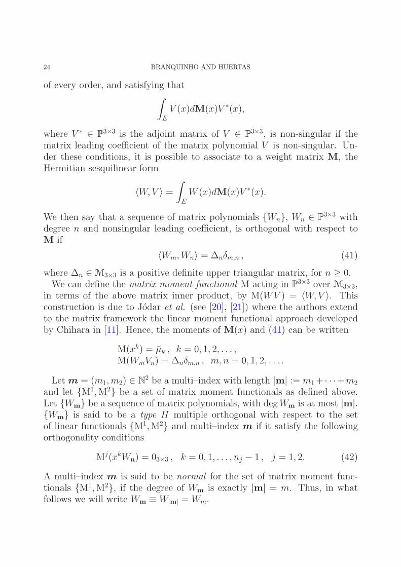
24 BRANQUINHO AND HUERTAS
of every order, and satisfying that∫
E
V (x)dM(x)V ∗(x),
where V ∗ ∈ P3×3 is the adjoint matrix of V ∈ P
3×3, is non-singular if thematrix leading coefficient of the matrix polynomial V is non-singular. Un-der these conditions, it is possible to associate to a weight matrix M, theHermitian sesquilinear form
〈W,V 〉 =
∫
E
W (x)dM(x)V ∗(x).
We then say that a sequence of matrix polynomials Wn, Wn ∈ P3×3 with
degree n and nonsingular leading coefficient, is orthogonal with respect toM if
〈Wm,Wn〉 = ∆nδm,n , (41)
where ∆n ∈ M3×3 is a positive definite upper triangular matrix, for n ≥ 0.We can define the matrix moment functional M acting in P
3×3 over M3×3,in terms of the above matrix inner product, by M(WV ) = 〈W,V 〉. Thisconstruction is due to Jodar et al. (see [20], [21]) where the authors extendto the matrix framework the linear moment functional approach developedby Chihara in [11]. Hence, the moments of M(x) and (41) can be written
M(xk) = µk , k = 0, 1, 2, . . . ,M(WmVn) = ∆nδm,n , m, n = 0, 1, 2, . . . .
Let m = (m1,m2) ∈ N2 be a multi–index with length |m| := m1+ · · ·+m2
and let M1,M2 be a set of matrix moment functionals as defined above.Let Wm be a sequence of matrix polynomials, with degWm is at most |m|.Wm is said to be a type II multiple orthogonal with respect to the setof linear functionals M1,M2 and multi–index m if it satisfy the followingorthogonality conditions
Mj(xkWn) = 03×3 , k = 0, 1, . . . , nj − 1 , j = 1, 2. (42)
A multi–index m is said to be normal for the set of matrix moment func-tionals M1,M2, if the degree of Wm is exactly |m| = m. Thus, in whatfollows we will write Wm ≡ W|m| = Wm.

SYMMETRIZATION PROBLEM IN MULTIPLE ORTHOGONALITY 25
In this framework, let consider the sequence of vector of matrix polynomialsBn where
Bn =
[W2n
W2n+1
]. (43)
We define the vector of matrix–functionals M =[M1 M2
]T, with M :
P6×3 → M6×6, by means of the action M on Bn, as follows
M (Bn) =
[M1(W2n) M2(W2n)M1(W2n+1) M2(W2n+1)
]∈ M6×6 . (44)
where
Mi(Wj) =
∫Wj(x)dM
i = ∆ij, i = 1, 2, and j = 0, 1, (45)
with dM1, dM2 being a system of two matrix of measures as describedabove. Thus, we say that a sequence of vectors of matrix polynomials Bnis orthogonal with respect to a vector of matrix functionals M if
i) M(xkBn) = 06×6 , k = 0, 1, . . . , n− 1 ,ii) M(xnBn) = Ωn ,
(46)
where Ωn is a regular block upper triangular 6× 6 matrix, holds.Now we are in a position to prove the following
Theorem 6 (Favard type). Let Bn a sequence of vectors of matrix polyno-mials of size 6×3, defined in (43), with Wn matrix polynomials satisfying thefour term recurrence relation (40). The following statements are equivalent:
(a) The sequence Bnn≥0 is orthogonal with respect to a certain vector oftwo matrix–functionals.
(b) There are sequences of scalar 6×6 block matrices A〈3〉n n≥0, B
〈3〉n n≥0,
and C〈3〉n n≥0, with C
〈3〉n block upper triangular non-singular matrix
for n ∈ N, such that the sequence Bn satisfy the matrix three termrecurrence relation
xBn = A〈3〉n Bn+1 +B〈3〉
n Bn + C〈3〉n Bn−1, (47)
with Bn−1 =[03×3 03×3
]T, B0 given, and C
〈3〉n non-singular.

26 BRANQUINHO AND HUERTAS
Proof : First we prove that (a) implies (b). Since the sequence of vector ofmatrix polynomials Bn is a basis in the linear space P
6×3, we can write
xBn =n+1∑
k=0
AnkBk, An
k ∈ M6×6 .
Then, from the orthogonality conditions (46), we get
M (xBn) = M(AnkBk) = 06×6, k = 0, 1, . . . , n− 2.
Thus,
xBn = Ann+1Bn+1 + An
nBn + Ann−1Bn−1 .
Having Ann+1 = A
〈3〉n , An
n = B〈3〉n , and An
n−1 = C〈3〉n , the result follows.
To proof that (b) implies (a), we know from Theorem 5 that the sequence ofvector polynomials Wn satisfy a four term recurrence relation with matrixcoefficients. We can associate this matrix four term recurrence relation (40)with the block matrix three term recurrence relation (47). Then, it is suffi-cient to show that M is uniquely determined by its orthogonality conditions
(46), in terms of the sequence C〈3〉n n≥0 in that (47).
Next, from (43) we can rewrite the matrix four term recurrence relation(40) into a matrix three term recurrence relation
xBn =
[03×3 03×3
A〈2〉2n+1 03×3
]Bn+1 +
[B
〈2〉2n A
〈2〉2n
C〈2〉2n+1 B
〈2〉2n+1
]Bn +
[D
〈2〉2n C
〈2〉2n
03×3 D〈2〉2n+1
]Bn−1,
where the size of Bn is 6×3. We giveM in terms of its block matrix moments,which in turn are given by the matrix coefficients in (47). There is a uniquevector moment functional M and hence two matrix measures dM1 and dM2,such that
M (B0) =
[M1(W0) M2(W0)M1(W1) M2(W1)
]= C
〈3〉0 ∈ M6×6,
where Mi(Wj) was defined in (45). For the first moment of M0 we get
M0 = M (B0) =
[∆1
0 ∆20
∆11 ∆2
1
]= C
〈3〉0 .
Hence, we haveM (B1) = 06×6, which from (47) also implies 06×6 = xM (B0)−
B〈3〉0 M (B0) = M1 − B
〈3〉0 M0. Therefore
M1 = B〈3〉0 C
〈3〉0 .
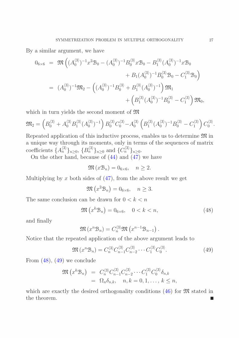
SYMMETRIZATION PROBLEM IN MULTIPLE ORTHOGONALITY 27
By a similar argument, we have
06×6 = M
((A
〈3〉0 )−1x2B0 − (A
〈3〉0 )−1B
〈3〉0 xB0 − B
〈3〉1 (A
〈3〉0 )−1xB0
+ B1(A〈3〉0 )−1B
〈3〉0 B0 − C
〈3〉1 B0
)
= (A〈3〉0 )−1
M2 −((A
〈3〉0 )−1B
〈3〉0 + B
〈3〉1 (A
〈3〉0 )−1
)M1
+(B
〈3〉1 (A
〈3〉0 )−1B
〈3〉0 − C
〈3〉1
)M0,
which in turn yields the second moment of M
M2 =(B
〈3〉0 + A
〈3〉0 B
〈3〉1 (A
〈3〉0 )−1
)B
〈3〉0 C
〈3〉0 −A
〈3〉0
(B
〈3〉1 (A
〈3〉0 )−1B
〈3〉0 − C
〈3〉1
)C
〈3〉0 .
Repeated application of this inductive process, enables us to determine M ina unique way through its moments, only in terms of the sequences of matrix
coefficients A〈3〉n n≥0, B
〈3〉n n≥0 and C
〈3〉n n≥0.
On the other hand, because of (44) and (47) we have
M (xBn) = 06×6, n ≥ 2.
Multiplying by x both sides of (47), from the above result we get
M(x2Bn
)= 06×6, n ≥ 3.
The same conclusion can be drawn for 0 < k < n
M(xkBn
)= 06×6, 0 < k < n, (48)
and finally
M (xnBn) = C〈3〉n M
(xn−1
Bn−1
).
Notice that the repeated application of the above argument leads to
M (xnBn) = C〈3〉n C
〈3〉n−1C
〈3〉n−2 · · ·C
〈3〉1 C
〈3〉0 . (49)
From (48), (49) we conclude
M(xkBn
)= C〈3〉
n C〈3〉n−1C
〈3〉n−2 · · ·C
〈3〉1 C
〈3〉0 δn,k
= Ωnδn,k, n, k = 0, 1, . . . , k ≤ n,
which are exactly the desired orthogonality conditions (46) for M stated inthe theorem.

28 BRANQUINHO AND HUERTAS
References[1] A.I. Aptekarev, Multiple orthogonal polynomials, J. Comput. Appl. Math. 99 (1998) 423–447.[2] A.I. Aptekarev, A. Branquinho, and W. Van Assche, Multiple orthogonal polynomials for
classical weights, Trans. Amer. Math. Soc. 335 (2003), 3887–3914.[3] A.I. Aptekarev, V. Kaliaguine, and J.V. Iseghem, Genetic sum’s representation for the mo-
ments of a system of Stieltjes functions and its application, Constr. Approx. 16 (2000), 487–524.
[4] A.I. Aptekarev, V.A. Kalyagin, and E.B. Saff, Higher-order three-term recurrences and asymp-totics of multiple orthogonal polynomials, Constr. Approx. 30 (2009), no. 2, 175–223.
[5] D. Barrios and A. Branquinho, Complex high order Toda and Volterra lattices, J. DifferenceEqu. Appl. 15 (2) (2009), 197–213.
[6] D. Barrios, A. Branquinho, and A. Foulquie-Moreno, Dynamics and interpretation of someintegrable systems via multiple orthogonal polynomials, J. Math. Anal. Appl. 361 (2) (2010),358–370.
[7] D. Barrios, A. Branquinho, and A. Foulqui-Moreno, On the relation between the full Kostant-Toda lattice and multiple orthogonal polynomials, J. Math. Anal. Appl. 377 (1) (2011), 228-238,
[8] D. Barrios, A. Branquinho, and A. Foulqui-Moreno, On the full Kostant-Toda system and thediscrete Korteweg-de Vries equations, J. Math. Anal. Appl. 401 (2) (2013), 811–820.
[9] B. Beckermann, On the convergence of bounded J-fractions on the resolvent set of the corre-sponding second order difference operator, J. Approx. Theory, 99 (2) (1999), 369–408.
[10] A. Branquinho, L. Cotrim, and A. Foulqui-Moreno, Matrix interpretation of multiple ortho-gonality, Numer. Algorithms 55 (2010) 19–37.
[11] T. S. Chihara, An Introduction to Orthogonal Polynomials. Mathematics and its ApplicationsSeries, Gordon and Breach, New York, 1978.
[12] S. Delvaux and A. Lpez–Garca, High order three-term recursions, Riemann-Hilbert minorsand Nikishin systems on star-like sets, Constr. Approx. (2012). In press.
[13] K. Douak and P. Maroni, Les polynomes orthogonaux “classiques” de dimension deux, Analysis12 (1992), 71-107.
[14] K. Douak and P. Maroni, Une caractrisation des polynmes d-orthogonaux classiques, J. Ap-prox. Th. 82 (1995) 177–204.
[15] A.J. Duran, On orthogonal polynomials with respect to a positive definite matrix of measures,Canad. J. Math. 47 (1995), 88–112.
[16] A.J. Duran and A. Grnbaum, A survey on orthogonal matrix polynomials satisfying secondorder differential equations, J. Comput. Appl. Math. 178 (2005), 169–190.
[17] M. Haneczok and W. Van Assche, Interlacing properties of zeros of multiple orthogonal poly-nomials, J. Math. Anal. Appl. 389 (1) (2012), 429–438.
[18] M.E.H. Ismail, Classical and quantum orthogonal polynomials in one variable, Encyclopediaof Mathematics and its Applications 98, Cambridge University Press, 2005.
[19] C.S. Gardner, J.M. Greene, M.D. Kruskal, and R.M. Miura, A method for solving theKorteweg–de Vries equation, Phys. Rev. Lett. 19 (1967) 1095–1097.
[20] L. Jdar and E. Defez, Orthogonal polynomials with respect to conjugate bilinear matrix momentfunctional: Basic theory, J. Approx. Theory Appl., 13 (1997), 66–79.
[21] L. Jdar, E. Defez, and E. Ponsoda, Orthogonal matrix polynomials with respect to linear matrixmoment functionals: theory and applications, J. Approx. Theory Appl., 12 (1996), 96–115.
[22] V. Kaliaguine, The operator moment problem, vector continued fractions and an explicit formof the Favard theorem for vector orthogonal polynomials, J. Comput. Appl. Math. 65 (1995)no. 1-3, 181–193.

SYMMETRIZATION PROBLEM IN MULTIPLE ORTHOGONALITY 29
[23] E. Isaacson and H. Bishop–Keller, Analysis of Numerical Methods, John Wiley & Sons, Inc.,New York, 1994.
[24] F. Marcellan and G. Sansigre, Quadratic decomposition of orthogonal polynomials: a matrixapproach, Numer. Algorithms 3 (1992) 285–298.
[25] P. Maroni and T.A. Mesquita, Cubic decomposition of 2–orthogonal polynomial sequences,Mediterr. J. Math. 10 (2013), 843–863.
[26] P. Maroni, T.A. Mesquita, and Z. da Rocha, On the general cubic decomposition of polynomialsequences, J. Difference Equ. Appl. 17 (9), (2011), 1303–1332.
[27] E.M. Nikishin and V.N. Sorokin, Rational approximants and orthogonality, vol. 92 in Trans-lations of Mathematical Monographs, Amer. Math. Soc., Providence, RI, 1991.
[28] F. Peherstorfer, On Toda lattices and orthogonal polynomials. Proceedings of the Fifth In-ternational Symposium on Orthogonal Polynomials, Special Functions and their Applications(Patras, 1999), J. Comput. Appl. Math. 133 (2001), no. 1-2, 519–534.
Amılcar Branquinho
CMUC and Department of Mathematics, University of Coimbra, Apartado 3008, EC Santa
Cruz, 3001-501 COIMBRA, Portugal.
E-mail address : [email protected]
Edmundo J. Huertas
CMUC and Department of Mathematics, University of Coimbra, Apartado 3008, EC Santa
Cruz, 3001-501 COIMBRA, Portugal.
E-mail address : [email protected]