Jorge Juan, 46, 28001, Madrid – España | Te..: +34 914 359 020 | Fax: +34 915 779 575 documentos.fedea.net | infpub@fedea.es

The Systematic Component of Monetary Policy in

SVARs: An Agnostic Identification Procedure

by

Jonas E. Arias*

Dario Caldara*

Juan F. Rubio-Ramírez**

Documento de Trabajo 2014-13

October 2014

* Federal Reserve Board.

** Duke University, BBVA Research, Federal Reserve Bank of Atlanta and FEDEA

Los Documentos de Trabajo se distribuyen gratuitamente a las Universidades e Instituciones de Investigación que lo solicitan. No obstante están

disponibles en texto completo a través de Internet: http://www.fedea.es.

These Working Paper are distributed free of charge to University Department and other Research Centres. They are also available through Internet:

http://www.fedea.es.

ISSN:1696-750

Fedea / non‐technical summary dt2014-13

NON‐‐‐‐TECHNICAL SUMMARY

En este trabajo analizamos como imponer restricciones en la parte

sistemática de la ecuación de política monetaria afecta a la estimación de modelos

estructurales de vectores autoregresivos. La mayoría de estos modelos son

estimados usando restricciones en las dinámicas de los efectos de los shocks

identificados. En este caso mostramos que los resultados cambian dramáticamente

una vez las restricciones se imponen en la parte sistemática de la política

monetaria.

Nuestros resultados contrastan con los de Uligh (2005). Uligh solo impone

restricciones en la dinámica de los shocks identificados y encuentra que la política

monetaria no es efectiva en sus efectos sobre el producto. Nosotros mostramos que

cuando las restricciones se imponen sobre la parte sistemática la política monetaria

si afecta al output y lo hace de la forma esperada. Un incremento de los tipos de

interés reduce el output.

The Systematic Component of Monetary Policy in

SVARs: An Agnostic Identification Procedure

Jonas E. Arias

Federal Reserve Board

Dario Caldara

Federal Reserve Board

Juan F. Rubio-Ramırez∗

Duke University, BBVA Research, and Federal Reserve Bank of Atlanta

September 10, 2014

Abstract

In this paper, we identify monetary policy shocks in structural vector autoregressions (SVARs)

by imposing sign and zero restrictions on the systematic component of monetary policy while

leaving the remaining equations in the system unrestricted. As in Uhlig (2005), no restrictions

are imposed on the response of output to a monetary policy shock. We find that an exogenous

increase in the federal funds rate leads to a persistent decline in output and prices. Our results

show that the contractionary effects of monetary policy shocks do not hinge on questionable

exclusion restrictions, but are instead consistent with agnostic identification schemes. The anal-

ysis is robust to various specifications of the systematic component of monetary policy widely

used in the literature.

∗Corresponding author: Juan F. Rubio-Ramırez <juan.rubio-ramirez@duke.edu>, Economics Department, DukeUniversity, Durham, NC 27708; 1-919-660-1865. We thank participants in seminars at the Atlanta Fed, PhiladelphiaFed, Board of Governorns of the Federal Reserve, IMF, University of Pennsylvania, and the Institute for EconomicAnalysis at the Universitat Autonoma de Barcelona for comments and discussions, especially Tony Braun, FrankDiebold, Pablo Guerron, Jesper Linde, Frank Schorfheide, Enrique Sentana, Pedro Silos, Rob Vigfusson, and TaoZha. The views expressed here are the authors’ and do not necessarily represent those of the Federal Reserve Bankof Atlanta or the Board of Governors of the Federal Reserve System. Juan F. Rubio-Ramırez also thanks the NSFfor support.

1 Introduction

Following Sims (1972, 1980, 1986), researchers have analyzed the effects of monetary policy on

output using structural vector autoregressions (SVARs). Most of them have concluded that an

increase in the federal funds rate or a decrease in the money supply are contractionary − i.e.,

they have a significant negative effect on output. The set of studies supporting this view includes

Bernanke and Blinder (1992); Christiano et al. (1996); Leeper et al. (1996); and Bernanke and

Mihov (1998).1 This intuitive result has become the cornerstone rationale behind New Keynesian

dynamic stochastic general equilibrium (DSGE) models. Researchers also estimate New Keynesian

models by matching the dynamic responses to a monetary policy shock implied by the model with

those implied by a SVAR − see Rotemberg and Woodford (1997) and Christiano et al. (2005).

The consensus about the contractionary effects of monetary policy shocks on output has been

challenged by Uhlig (2005), who found no evidence to support such a view using an agnostic

identification strategy. Uhlig’s (2005) critique is that traditional SVARs require the researcher to

identify all shocks in the system and impose a tremendous number of possibly spurious restrictions.

He therefore proposes to identify monetary policy shocks by imposing sign restrictions on just the

impulse response functions of prices and nonborrowed reserves to the shock. These restrictions

eliminate the well-known price and liquidity puzzles while remaining agnostic about the responses

of other variables, particularly output, to the monetary policy shock.2 Furthermore, this approach

does not restrict the response of any variable to the remaining structural shocks. This means that

Uhlig (2005) does not identify a single model but rather a set of models that are coherent with

his sign restrictions. In other words, he does not identify the structural parameters themselves but

instead set-identifies them.

In this paper, we endorse the agnostic approach, but instead of imposing restrictions on impulse

response functions to a monetary policy shock, we impose them on the monetary policy equation.

In particular, we use an agnostic identification scheme to restrict the systematic component of

monetary policy. Our approach is inspired by the line of work of Leeper et al. (1996); Leeper

1Leeper et al. (1996), Bagliano and Favero (1998), and Christiano et al. (1999) survey this extensive literature.2See Sims (1992) for a description of the price puzzle, and Leeper and Gordon (1992) for a description of the

liquidity puzzle.

1

and Zha (2003); and Sims and Zha (2006a), which emphasizes the need to specify and estimate

behavioral relationships for monetary policy. Policy choices in general, and monetary policy choices

in particular, do not evolve independently of economic conditions: even the harshest critics of

monetary authorities would not maintain that policy decisions are unrelated to the economy (Leeper

et al., 1996). Thus, to isolate exogenous changes in policy, one needs to model how policy reacts

to the economy.

We identify monetary policy shocks by imposing sign and zero restrictions on the systematic

component of monetary policy. We propose three alternative sets of restrictions, inspired by three

specifications of the systematic component that are widely used in the literature. The first specifi-

cation derives from standard SVARs, such as the one prominently used by Christiano et al. (1996),

and implies that the federal funds rate responds positively to output and prices. The second speci-

fication originates from Taylor-type rules widely used in DSGE models and implies that the federal

funds rate responds to inflation and a measure of economic activity. The third specification con-

siders the class of money rules described in Leeper et al. (1996); Leeper and Zha (2003); and Sims

and Zha (2006a,b). In contrast to these papers, we set-identify the SVAR because we only impose

sign and zero restrictions on the monetary policy equation and we leave the non-policy equations

unrestricted. Hence, our approach shares two features with Uhlig (2005). First, we do not impose

any restriction on the response of output to monetary shocks. Second, we do not identify a single

model but rather a set of models that are coherent with our sign and zero restrictions.

We highlight two results. First, we find that an exogenous increase in the federal funds rate has

persistent contractionary effects on output. The decline in real activity, together with the decline

in prices, causes a medium-term loosening of the monetary policy stance. Hence, our agnostic

identification scheme recovers the consensus regarding the effects of monetary policy shocks while

addressing Uhlig (2005)’s critique. Second, we show that the identification scheme in Uhlig (2005)

violates our restrictions on the systematic component of monetary policy. Following Leeper et al.

(1996); Leeper and Zha (2003); and Sims and Zha (2006a), a corollary to our findings is that the

shocks identified in Uhlig (2005) are not monetary policy shocks because the systematic component

of monetary policy is counterfactual and does not control for the endogenous response of monetary

2

policy to economic activity.

To further understand the relationship between the identification schemes, we combine the sign

restrictions on impulse response functions in Uhlig (2005) with our restrictions on the systematic

component. We find that our restrictions substantially shrink the set of models originally identified

by Uhlig (2005), and that excluding models with counterfactual monetary policy equations suffices

to generate a negative response of output and thereby recover the consensus. The restrictions in

Uhlig (2005) also refine the set of admissible models obtained using our approach, as they exclude

models that generate the price puzzle. But this refinement has modest impact on the results, as

the subset of excluded models is small.

Our work is related to several studies in the literature. A similar identification strategy to the

one used in this paper is employed in Caldara and Kamps (2012), who identify tax and govern-

ment spending shocks by putting discipline on the systematic component of fiscal policy. They

combine zero restrictions with empirically plausible bounds on the output elasticities of fiscal vari-

ables. Baumeister and Hamilton (2014) study how informative are the data relative to the prior

distributions in the estimation of SVARs. In one of their examples they impose prior distributions

on the systematic component of monetary policy of a very simple three equations model. Arias

et al. (2014) develop the theoretical foundation to identify SVARs by jointly imposing sign and

zero restrictions. They apply their methodology to revisit the identification of optimism shocks in

Beaudry et al. (2011) and the identification of fiscal shocks in Mountford and Uhlig (2009). Both

applications impose restrictions on impulse response functions, while we apply their methodology

to impose restrictions directly on the SVAR equations. We also study identification schemes that

combine restrictions on the SVAR equations with restrictions on impulse response functions. Some

recent applications of SVAR identification based on sign and zero restrictions on impulse response

functions include Baumeister and Benati (2010), who identify the effects of unconventional mone-

tary policy; Binning (2013), who identifies anticipated government spending shocks; and Peersman

and Wagner (2014), who identify shocks to bank lending.

The structure of the paper is as follows. In Section 2, we describe the SVAR methodology

and describe our baseline identification scheme. In Section 3, we describe the results and compare

3

them with Uhlig (2005). In Section 4, we consider alternative specifications of the monetary policy

equation. In Section 5, we conclude.

2 Methodology

Let us consider the following SVAR

y′tA0 =

p∑`=1

y′t−`A` + c + ε′t for 1 ≤ t ≤ T, (1)

where yt is an n × 1 vector of endogenous variables, εt is an n × 1 vector of structural shocks,

A` is an n × n matrix of structural parameters for 0 ≤ ` ≤ p with A0 invertible, c is a 1 × n

vector of parameters, p is the lag length, and T is the sample size. The vector εt, conditional on

past information and the initial conditions y0, ...,y1−p, is Gaussian with mean zero and covariance

matrix In (the n× n identity matrix). The model described in equation (1) can be written as

y′tA0 = x′tA+ + ε′t for 1 ≤ t ≤ T, (2)

where A′+ =

[A′1 · · · A′p c′

]and x′t =

[y′t−1 · · · y′t−p 1

]for 1 ≤ t ≤ T . The dimension

of A+ is m×n, where m = np+1. We call A0 and A+ the structural parameters. The reduced-form

representation implied by equation (2) is

y′t = x′tB + u′t for 1 ≤ t ≤ T,

where B = A+A−10 , u′t = ε′tA−10 , and E [utu

′t] = Σ = (A0A

′0)−1. The matrices B and Σ are the

reduced-form parameters. Finally, the impulse response functions (IRFs) are as follows.

Definition 1. Let (A0,A+) be any value of structural parameters, the IRF of the i-th variable to

the j-th structural shock at finite horizon h corresponds to the element in row i and column j of

4

the matrix

Lh (A0,A+) =(A−10 J′FhJ

)′, where F =

A1A−10 In · · · 0

......

. . ....

Ap−1A−10 0 · · · In

ApA−10 0 · · · 0

and J =

In

0

...

0

.

Papers in the literature involving set identification of structural parameters typically impose

sign and/or zero restrictions on either A0 or the IRFs. The identification approach that we propose

in this paper combines sign and zero restrictions on A0 or IRFs or both. We use restrictions on A0

to discipline the systematic component of monetary policy and restrictions on the IRFs to restrict

the dynamics of the structural shocks.

Our methodology is based on Rubio-Ramırez et al. (2010) and Arias et al. (2014). For details,

we refer the reader to the mentioned papers, but we can summarize the characterization of the

restrictions as follows. Let us assume that we want to impose restrictions on some elements of

A0 and on some IRFs at different horizons. It is convenient to stack A0 and the IRFs for all the

relevant horizons into a single matrix of dimension k × n, which we denote by f (A0,A+). For

example, if we impose restrictions at horizons zero and one, then

f (A0,A+) =

A0

L0 (A0,A+)

L1 (A0,A+)

, where k = 3n in this case.

We represent the sign restrictions on f (A0,A+) used to identify structural shock j by a matrix

Sj , where the number of columns in Sj is equal to k and 1 ≤ j ≤ n. Sj is a selection matrix

and thus has one non-zero entry in each row. If the rank of Sj is sj , then sj is the number of

sign restrictions imposed to identify the j − th structural shock. Similarly, we represent the zero

restrictions on f (A0,A+) used to identify structural shock j by selection matrices Zj , where the

number of columns in Zj is also equal to k and each row has one non-zero entry. If the rank

of Zj is zj , then zj is the number of zero restrictions imposed to identify the j − th structural

5

shock. When we only impose sign restrictions, we draw from the posterior distribution of the

structural parameters using algorithms in Rubio-Ramırez et al. (2010). When we impose sign and

zero restrictions, we draw using algorithms in Arias et al. (2014).

To highlight the implications of our identification scheme, we choose a widely used specification

of the reduced-form VAR model. In particular, we make our results comparable to Uhlig (2005),

and we use Bayesian methods to estimate the same reduced-form model as Uhlig (2005) on his

dataset, which spans U.S. monthly data from 1965:I to 2003:XII, using his priors. Given that the

priors, the reduced-form model, and the data have been extensively discussed by Uhlig (2005), for

our purposes it suffices to mention that the VAR specification includes output (real GDP), yt; the

GDP deflator, pt; an index of commodity prices; pc,t; total reserves, trt; nonborrowed reserves,

nbrt; and the federal funds rate, rt. We take the natural logarithm of all variables except for the

federal funds rate, and without loss of generality, we assume in all our identification schemes that

variables follow the order of listing above. This vector of endogenous variables is standard in the

literature and has been used, among others, by Christiano et al. (1996) and Bernanke and Mihov

(1998). The VAR specification includes 12 lags (p = 12) and does not include any deterministic

term.3

2.1 Sign Restrictions on IRFs

Agnostic identification schemes are commonly associated with the imposition of sign restrictions

on IRFs. A seminal paper in this literature is Uhlig (2005). This paper examines the effects of

monetary policy shocks on output. In order to identify monetary policy shocks, he imposes the

following restrictions.

Restriction 1. A monetary policy shock leads to a negative response of the GDP deflator, com-

modity prices, and nonborrowed reserves, and to a positive response of the federal funds rate, all at

horizons t = 0, . . . , 5.

Restriction 1 rules out the price puzzle —a positive response of the price level following a mon-

etary contraction— and the liquidity puzzle —a positive response of monetary aggregates. Uhlig

3We repeat the analysis using an updated version of the dataset running until 2007, and a version with quarterlydata. Results reported in the following sections are robust to the use of these datasets and are available upon request.

6

(2005) motivates these restrictions as a way to rule out implausible price and reserve behaviors, so

that the set of admissible SVARs does not include models that we would find not interesting from a

theoretical perspective. Restriction 1 implies non-linear restrictions on (A0,A+). But the crucial

features of the identification described by Restriction 1 are that (i) it remains agnostic about the

response of output after an increase in the federal funds rate and (ii) it only identifies monetary

policy shocks. This implies that Restriction 1 does not identify the structural parameters but only

set-identifies them, allowing a set of models, rather than a single model, to be compatible with the

restrictions.

Without loss of generality, if we let the monetary policy shock be the first structural shock, we

characterize Restriction 1 with the matrices described below.4

f (A0,A+) =

L0 (A0,A+)

...

L5 (A0,A+)

, S1 =

S10 0m,n . . . 0m,n

0m,n. . .

. . ....

.... . .

. . . 0m,n

0m,n · · · 0m,n S15

, and

S1t =

0 −1 0 0 0 0

0 0 −1 0 0 0

0 0 0 0 −1 0

0 0 0 0 0 1

for t = 0, . . . , 5, where m = 6 and n = 4.

In Figure 1, we plot the IRFs to an exogenous tightening of monetary policy identified by

imposing Restriction 1. Throughout the paper, we normalize the size of the shock to be equal to

one standard deviation. All results are based on 10, 000 draws from the posterior distribution of

the structural parameters. The shadowed area shows the 68% confidence bands and the solid lines

show the median IRFs. This figure replicates Figure 6 in Uhlig (2005). Panel (A) shows that the

median response of output is positive. In addition, there is evidence that in the short run the 68%

4In the paper, it is always the case that the monetary policy shock is the first structural shock.

7

confidence bands do not contain zero. Panels (B) and (C) show the response of the GDP deflator

and the commodity price index, respectively, which are restricted to be negative for six months to

exclude the price puzzle. Panels (D) and (E) show the response of total reserves and nonborrowed

reserves, both of which are negative in the short run. The reduction in nonborrowed reserves is

more significant because the response of this variable is restricted to be negative for six months to

exclude the liquidity puzzle. Finally, Panel (F) shows the response of the federal funds rate, which

is restricted to be positive for the first six months and it becomes negative 18 months after the

shock.

Figure 1: IRFs to a Monetary Policy Shock Identified Using Restrictions 1

Hence, consistent with Uhlig (2005), the main result shown in Figure 1 is the lack of support

for the contractionary effects on output of an exogenous increase in the federal funds rate. This

result presents a challenge to the consensus view that output decreases in response to a tightening

of monetary policy. Replicating Uhlig (2005) is important because in the next section we show

that, despite its appeal, Restriction 1 implies a counterfactual systematic component of monetary

8

policy and therefore does not identify monetary policy shocks.

2.2 Systematic Component of Monetary Policy

The identification of monetary policy shocks either requires or implies the specification of how policy

usually reacts to economic conditions. Leeper et al. (1996); Leeper and Zha (2003); and Sims and

Zha (2006a) emphasize the need to specify and estimate the behavior of the systematic component

of monetary policy. Uhlig (2005) deviates from this paradigm, as discussed in the previous section,

but we argue that the implied systematic component provides a useful way to check whether the

set of identified models is a sensible one.

In order to characterize the systematic component of monetary policy, it is important to note

that labeling a structural shock in the SVAR as the monetary policy shock is equivalent to specifying

the same equation as the monetary policy equation. Thus, the first equation of the SVAR,

y′ta0,1 =

p∑`=1

y′t−`a`,1 + ε1t for 1 ≤ t ≤ T, (3)

is the monetary policy equation, where ε1t denotes the first entry of εt, a`,1 denotes the first column

of A` for 0 ≤ ` ≤ p, and a`,ij denotes the (i, j) entry of A`. Consequently,∑p

`=1 y′t−`a`,1 describes

the systematic component of monetary policy.

When analyzing the systematic component of monetary policy, we borrow from the literature

three specifications of the monetary policy equation. The benchmark specification, discussed in this

section, is motivated by Christiano et al. (1996). The second and third specifications, discussed

in Section 4, are motivated, respectively, by Taylor (1993, 1999); and Leeper et al. (1996); Leeper

and Zha (2003); Sims and Zha (2006a); and Sims and Zha (2006b). Even though each of these

approaches characterizes the systematic component of monetary policy in a particular way, they

deliver similar results.

The monetary policy equation implied by Christiano et al. (1996) makes two important iden-

tification assumptions about the systematic component of monetary policy. They are summarized

as follows.

9

Restriction 2. The federal funds rate is the monetary policy instrument and it only reacts con-

temporaneously to output and prices.

Restriction 2 comprises two parts. First, the fact that the federal funds rate is the policy

instrument is supported by empirical and anecdotal evidence. Except for a short period between

October 1979 and October 1982 when the Federal Reserve explicitly targeted nonborrowed reserves,

monetary policy in the U.S. since 1965 can be characterized by a direct or indirect interest rate

targeting regime.5 Sims and Zha (2006b) also provide support for this view in their finding that

the federal funds rate was the policy instrument for most of their sample, which runs from 1959 to

2003. Even so, they also suggest that one should be careful when applying the Taylor formalism to

interpret specific historical periods; for example, as in Bernanke and Blinder (1992), they find that

policy behavior was better characterized by nonborrowed reserves targeting in the first three years

of Paul Volcker’s tenure as Chairman of the Federal Reserve from October 1979 to October 1982,

as well as in the first years of Arthur Burns’ tenure as Chairman of the Fed in the early 1970s.

With these exceptions in mind, one could conclude that the Fed has used the federal funds rate as

its monetary policy instrument almost continuously since 1965, although the federal funds rate has

only formally been the Federal Reserve’s policy instrument since 1997.

Second, the federal funds rate does not react to changes in reserve aggregates. Bernanke and

Blinder (1992) and Christiano et al. (1996) include reserve aggregates because in the mid-1990s

they were viewed as alternative instruments for characterizing the conduct of monetary policy.

Nevertheless, when the federal funds rate is the monetary instrument in these papers, reserve

aggregates do not enter the monetary equation.6

Next, we impose qualitative restrictions on the response of the federal funds rate to economic

conditions, which we summarize as follows.

Restriction 3. The contemporaneous reaction of the federal funds rate to output and prices is

nonnegative.

5See Bernanke and Blinder (1992) and Chappell Jr et al. (2005).6Christiano et al. (1996) study also a monetary rule where nonborrowed reserves is the policy instrument. We do

not explore this specification because the analysis in Christiano et al. (1996) is not robust to extending the samplebeyond 1995. This is consistent with the view that nonborrowed reserves were used as an explicit policy instrumentonly in the early 1980s.

10

Restriction 3 is implicit in the Federal Reserve Act, according to which the objectives of mone-

tary policy are maximum employment, stable prices, and moderate long-term interest rates. From

a more general perspective, it is a reflection of the modern conduct of monetary policy, which is less

mechanical than it was at the beginning of 20th century, and is based instead on achieving certain

economic goals, such as full employment and price stability, as mentioned above (see Woodford

(2003)).

We see the set of behavioral policy equations that are consistent with Restriction 2 and 3 as

the largest set describing the historical conduct of U.S. monetary policy toward fulfilling these

objectives. Importantly, we stress that Restrictions 2 and 3 are sign and zero restrictions on the

coefficients of the monetary policy equation and they do not impose restrictions on the response

of variables to the monetary policy shocks, nor restrict the sign of such responses. For this reason,

we remain agnostic about the response of output to an increase in the federal funds rate. It is also

the case that, contrary to Christiano et al. (1996), we leave the remaining equations unrestricted

and therefore only identify monetary policy shocks. Thus, as in Uhlig (2005), Restrictions 2 and

3 do not identify the structural parameters but only set identify them, allowing a set of models to

be compatible with the restrictions rather than a single one.7

If we only concentrate on the contemporaneous coefficients, we can rewrite equation (3) as

rt = ψyyt + ψppt + ψpcpc,t + ψtrtrt + ψnbrnbrt + a−10,61ε1,t (4)

where ψy = a−10,61a0,11, ψp = a−10,61a0,21, ψpc = a−10,61a0,31, ψtr = a−10,61a0,41, and ψnbr = a−10,61a0,51.

Equipped with this representation of the monetary policy equation, we describe Restrictions 2 and

3 as follows.

Remark 1. Restriction 2 implies that ψtr = ψnbr = 0, while Restriction 3 implies that ψy, ψp, ψpc ≥

0.

Let s10, the number of sign restrictions at horizon 0, be equal to 5, s1+, the number of sign

restrictions at horizon greater than 1, be equal to 1, and z10, the number of zero restrictions at

7See Arias et al. (2014) for details on set identification in SVARs identified imposing sign and zero restrictions.

11

horizon zero, be equal to 2. If we let the monetary policy shock be the first structural shock,

then Restrictions 2 and 3 and the normalization on the federal funds rate impose restrictions on

(A0,A+) that are characterized using the following matrices.

f (A0,A+) =

A0

L0 (A0,A+)

...

L5 (A0,A+)

, S1 =

S10 0s10,n . . . 0s10,n

0s1+,2n S11 0s1+,n . . .

... 0m,n. . .

...

0s1+,2n... . . . S15

,

Z1 =

[Z10 0z10,5n

], S10 =

−1 0 0 0 0 0 01,n

0 −1 0 0 0 0...

0 0 −1 0 0 0...

0 0 0 0 0 1 01,n

0s,1 . . . . . . . . . . . . 0s,1 S

, S ≡

0

0

0

0

0

1

′

,

S1t = S for t = 1, . . . , 5, and Z10 =

0 0 0 1 0 0 0 0 0 0 0 0

0 0 0 0 1 0 0 0 0 0 0 0

.We impose two normalizations. First, when we impose Restrictions 2 and 3 only, we normalize

the sign of the shock by assuming that the federal funds rate response remains positive for six

months.8 Second, we restrict a0,61 > 0 in order to satisfy the regularity conditions for f (A0,A+)

specified in Arias et al. (2014).

In Section 3, we present results for the identification of monetary policy shocks that jointly

imposes Restrictions 1, 2, and 3 on (A0,A+). To characterize this identification scheme, it suffices

8We choose six months as our baseline because there is ample evidence of short-run smoothing of policy rates(Rudebusch, 2006). Results are robust to imposing this normalization for both one and three months. We also applythis normalization to the policy rules considered in Section 4.

12

to modify the above set of matrices by setting s10 = 8, s1+ = 3, and matrix S to

S =

0 −1 0 0 0 0

0 0 −1 0 0 0

0 0 0 0 −1 0

0 0 0 0 0 1

.

3 Results

In this section, we characterize the systematic component of monetary policy implied by Uhlig’s

(2005) identification scheme and highlight the fact that it is counterfactual. We then present results

for our agnostic identification scheme based on Restrictions 2 and 3.

3.1 Systematic Component of Monetary Policy and Uhlig (2005)

We now describe the systematic component of monetary policy that is consistent with the monetary

policy shocks identified in Uhlig (2005). By construction, the set of models that satisfy Restriction

1 implies ψtr 6= 0 and ψnbr 6= 0, thus violating Restrictions 2. As explained in Arias et al. (2014),

unless we condition on the zero restrictions to draw the structural parameters, the set of models

that satisfy such zero restrictions has measure zero. More importantly, we show in Figure 2 that

Restriction 1 also implies coefficients on output (ψy) and prices (ψp and ψpc) that violate Restriction

3. Panels (A), (B), and (C) show the cumulative density functions (CDFs) of the coefficients ψy,

ψp, and ψpc . The y-axes indicate the value of the CDFs and the x-axes indicate the support of

these distributions. Restriction 1 allocates a significant probability mass to negative values of these

coefficients and, as a byproduct, to events in which there is a monetary tightening in response to

a decrease in either prices or output. Over 60% of the draws violate the sign restriction on ψy,

about 15% of the draws violate the sign restriction on ψp, and 10% of the draws violate the sign

restriction on ψpc . 80% of the draws violate at least one sign restriction and, as explained in the

previous paragraph, all draws violate the sign and zero restrictions.

This exercise shows that Uhlig’s (2005) identification scheme implies a counterfactual systematic

13

−2000 0 2000

0.25

0.5

0.75

1

ψy

(A): Output

−2000 0 2000

0.25

0.5

0.75

1

ψp

(B): GDP Deflator

−500 0 500

0.25

0.5

0.75

1

ψpc

(C): Commodity Price Index

Figure 2: Systematic Component of Monetary Policy Implied by Uhlig (2005)

component of monetary policy that violates both Restrictions 2 and 3. Following Leeper et al.

(1996); Leeper and Zha (2003); and Sims and Zha (2006a), a corollary to our findings is that the

shocks identified by Restriction 1 are not monetary policy shocks because the systematic component

of monetary policy is counterfactual and hence does not control for the endogenous response of

monetary policy to economic activity as characterized by Restrictions 2 and 3.

3.2 Restricting the Systematic Component of Monetary Policy

We now present results derived by imposing Restrictions 2 and 3 on the monetary policy equation.

We first combine those restrictions with the sign restrictions in Uhlig (2005) before applying them

in isolation.9

In Figure 3, we plot the IRFs to a monetary policy shock identified by jointly imposing Restric-

tions 1, 2, and 3. We emphasize two results. First, the output response is negative and it builds

up over time.10 Second, the contour of the federal funds rate is similar to Uhlig (2005): positive

for one year, and negative thereafter. But contrary to Uhlig (2005), we can rationalize this path

with the systematic component of monetary policy, as the drop in the federal funds rate is the

endogenous response of policy to the decline in real activity and prices.

9As explained in Section 2.2, we normalize the response of the federal funds rate response to be positive when weapply Restrictions 2 and 3 in isolation, as this sign normalization is implicit in Restrictions 1. This is also the casein Section 4.

10As mentioned in Section 2.2, this identification scheme remains silent about the effects of output to a monetarypolicy shock.

14

Figure 3: IRFs to a Monetary Policy Shock Identified Using Restrictions 1, 2, and 3

Finally, in Figure 4 we plot the IRFs to a monetary shock identified by imposing only Restric-

tions 2 and 3. Dropping Restriction 1 has little effect on our main finding: output drops following

monetary tightening and, together with a drop in prices, leads to a long-run loosening of the policy

stance. But Panel (B) shows that dropping Restriction 1 leads to the emergence of the price puzzle,

though one of quantitatively modest size. Hence, the set of models characterized by Restrictions 2

and 3 include a small subset of models with a counterfactual response of prices to monetary shocks.

Comparing Figures 3 and 4, we see that Restriction 1 helps refining the set of models by excluding

models that generate the price puzzle, although the effect of imposing Restriction 1 on the IRFs is

quantitatively modest.11

It is also important to highlight that our results in Figures 3 and 4 contradict Uhlig’s (2005)

claim that you need to restrict the initial response of output to zero in order to recover the consensus.

In both figures the initial response is different from zero and output drops after the negative

11To eliminate the price puzzle we would only need to impose that a monetary policy shock leads to a negativeresponse of the GDP deflator, without imposing the remaining sign restrictions described in Restriction 1.

15

monetary policy shock.

Figure 4: IRFs to a Monetary Policy Shock Identified Using Restrictions 2 and 3

All told, three messages emerge from this section. First, imposing some discipline in the sys-

tematic component of monetary policy is crucial to recover the conventional effects of monetary

policy. Second, once the systematic behavior of monetary policy is restricted, imposing additional

sign restrictions on IRFs as motivated by Uhlig (2005) helps refine the set of admissible models but

is not crucial for the results. Third, it is not necessary to have a dogmatic zero restriction on the

output response to a monetary policy shock in order to rescue the conventional effects of monetary

policy.

4 Alternative Systematic Components of Monetary Policy

In this section, we consider two alternative specifications of the monetary policy equation. The

first specification is a rule motivated by the use in DSGE models of interest rate rules reacting to

inflation and some measure of economic activity. We refer to this class of rules as Taylor rules.

16

The second rule is a money rule motivated by the work of Leeper et al. (1996); Leeper and Zha

(2003); Sims and Zha (2006a); and Sims and Zha (2006b). Each of these specifications has received

wide attention in the empirical monetary literature and provides alternative descriptions of the

systematic component.

4.1 Taylor-Type Rule

In the specification of the monetary policy equation studied in Section 2, the federal funds rate

responds to output and price levels. But researchers, especially those working with DSGE models,

often consider Taylor-type monetary policy equations in which the funds rate responds to inflation

and a measure of economic activity instead. Inspired by the Taylor rules used in the literature, we

model the systematic component of monetary policy using the following set of restrictions.

Restriction 4. The federal funds rate is the monetary policy instrument and it only reacts con-

temporaneously to output growth, GDP deflator inflation, and commodity prices inflation.

Restriction 5. The contemporaneous reaction of the federal funds rate to output growth and both

measures of inflation is nonnegative.

We specify a rule in the growth rate of output and not in the output gap (or the growth rate

of the output gap) as done in many DSGE models because our reduced-form specification does not

include potential output. However, results are qualitatively similar for a specification that includes

output instead of its growth rate.

As in Section 2, since Restrictions 4 and 5 just describe sign and zero restrictions on the

coefficients of the monetary policy equation, we remain agnostic about the response of output to

a monetary policy shock. These restrictions only identify the behavior of the monetary policy

equation while leaving the remaining equations unrestricted.12

12In this exercise, while we set-identify the structural parameters, we exactly identify the IRFs associated withthe monetary policy shock. That is, for any draw of the reduced-form parameters, there exists at most one columnof the rotation matrix that satisfies the sign and zero restrictions. This is the case because in the Taylor-type ruleidentification scheme we impose n − 1 zero restrictions on the monetary policy equation. If we relax the sign andzero restrictions on commodity price inflation, the IRFs to a monetary shock are set-identified and are very similarto those reported in Figures 5 and 6. See Arias et al. (2014) for additional details.

17

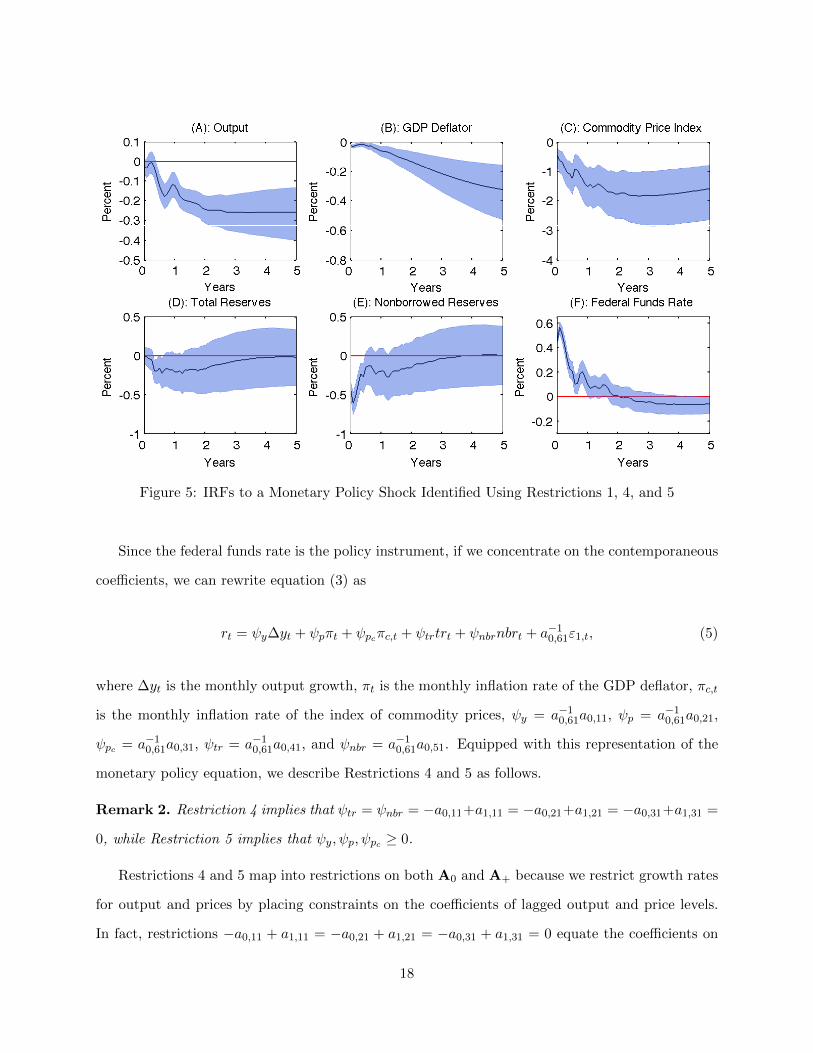
Figure 5: IRFs to a Monetary Policy Shock Identified Using Restrictions 1, 4, and 5

Since the federal funds rate is the policy instrument, if we concentrate on the contemporaneous

coefficients, we can rewrite equation (3) as

rt = ψy∆yt + ψpπt + ψpcπc,t + ψtrtrt + ψnbrnbrt + a−10,61ε1,t, (5)

where ∆yt is the monthly output growth, πt is the monthly inflation rate of the GDP deflator, πc,t

is the monthly inflation rate of the index of commodity prices, ψy = a−10,61a0,11, ψp = a−10,61a0,21,

ψpc = a−10,61a0,31, ψtr = a−10,61a0,41, and ψnbr = a−10,61a0,51. Equipped with this representation of the

monetary policy equation, we describe Restrictions 4 and 5 as follows.

Remark 2. Restriction 4 implies that ψtr = ψnbr = −a0,11+a1,11 = −a0,21+a1,21 = −a0,31+a1,31 =

0, while Restriction 5 implies that ψy, ψp, ψpc ≥ 0.

Restrictions 4 and 5 map into restrictions on both A0 and A+ because we restrict growth rates

for output and prices by placing constraints on the coefficients of lagged output and price levels.

In fact, restrictions −a0,11 + a1,11 = −a0,21 + a1,21 = −a0,31 + a1,31 = 0 equate the coefficients on

18

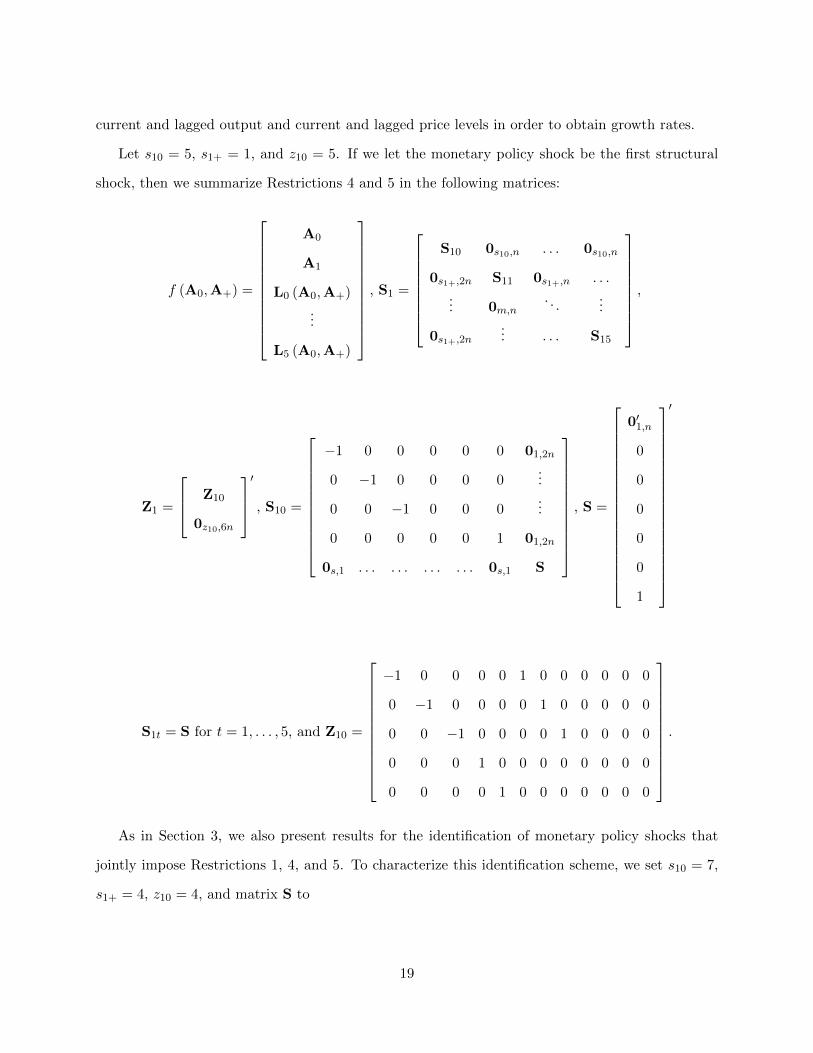
current and lagged output and current and lagged price levels in order to obtain growth rates.

Let s10 = 5, s1+ = 1, and z10 = 5. If we let the monetary policy shock be the first structural

shock, then we summarize Restrictions 4 and 5 in the following matrices:

f (A0,A+) =

A0

A1

L0 (A0,A+)

...

L5 (A0,A+)

, S1 =

S10 0s10,n . . . 0s10,n

0s1+,2n S11 0s1+,n . . .

... 0m,n. . .

...

0s1+,2n... . . . S15

,

Z1 =

Z10

0z10,6n

′

, S10 =

−1 0 0 0 0 0 01,2n

0 −1 0 0 0 0...

0 0 −1 0 0 0...

0 0 0 0 0 1 01,2n

0s,1 . . . . . . . . . . . . 0s,1 S

, S =

0′1,n

0

0

0

0

0

1

′

S1t = S for t = 1, . . . , 5, and Z10 =

−1 0 0 0 0 1 0 0 0 0 0 0

0 −1 0 0 0 0 1 0 0 0 0 0

0 0 −1 0 0 0 0 1 0 0 0 0

0 0 0 1 0 0 0 0 0 0 0 0

0 0 0 0 1 0 0 0 0 0 0 0

.

As in Section 3, we also present results for the identification of monetary policy shocks that

jointly impose Restrictions 1, 4, and 5. To characterize this identification scheme, we set s10 = 7,

s1+ = 4, z10 = 4, and matrix S to

19

S =

01,n 0 −1 0 0 0 0

... 0 0 −1 0 0 0

... 0 0 0 0 −1 0

01,n 0 0 0 0 0 1

.

In Figure 5, we plot the IRFs to a monetary policy shock identified by imposing Restrictions

1, 4, and 5. Qualitatively, the results are similar to those obtained using Restrictions 1, 2, and

3: output declines after a negative monetary policy shock, and monetary policy loosens its stance

in the long run. But all the IRFs, particularly the output response, are more precisely estimated

which reinforces the message that a negative monetary policy shock is contractionary once the

systematic component of monetary policy is taken into account.

In Figure 6, we plot the IRFs to a monetary policy shock identified by imposing only Restrictions

4 and 5, together with the sign normalization on the response of the federal funds rate. As in Section

3, dropping Restriction 1 leads to the emergence of the price puzzle. Nevertheless, the response of

output to the monetary tightening is negative and persistent. The response of the other variables

is also similar to Figure 5.

The analysis confirms the robustness of our findings. This alternative agnostic identification

scheme that restricts the systematic behavior of monetary policy is consistent with the consensus

regarding the effects of monetary policy on output. Imposing additional sign restrictions on IRFs

as motivated by Uhlig (2005) helps to refine the set of admissible models that are consistent with

the systematic component of monetary policy, but it is not crucial for the results.

4.2 Money Rule

Finally, the last specification of the monetary policy equation that we consider follows the money

rules postulated in Leeper et al. (1996); Leeper and Zha (2003); and Sims and Zha (2006a,b). In

these rules, only the federal funds rate and money enter the monetary policy equation. To model

this rule, we follow Sims and Zha (2006b) and replace total reserves and nonborrowed reserves with

20

Figure 6: IRFs to a Monetary Policy Shock Identified Using Restrictions 4 and 5

money, as measured by M2.13 Except for this use of money instead of reserves, the reduced-form

model is identical to the one we describe in Section 2.

We first replicate the main findings in Uhlig (2005) using the new reduced-form specification in

order to show that his results are not a consequence of using reserves instead of money. To imple-

ment Uhlig’s (2005) agnostic identification scheme, we replace the sign restrictions on nonborrowed

reserves with sign restrictions on money. We thus characterize the agnostic identification scheme

by the following Restriction.

Restriction 6. A monetary policy shock leads to a negative response of the GDP deflator, com-

modity prices, and money, and to a positive response of the federal funds rate, all at horizons

t = 0, . . . , 5.

As was the case with Restriction 1, Restriction 6 rules out the price and the liquidity puzzles and

implies non-linear restrictions on (A0,A+). But the crucial feature of the identification described

13We use monthly data on M2 Money supply (M2SL) from the H.6 Money supply Measures of the Board ofGovernors of the Federal Reserve System downloaded from the Federal Reserve Bank of Saint Louis.

21

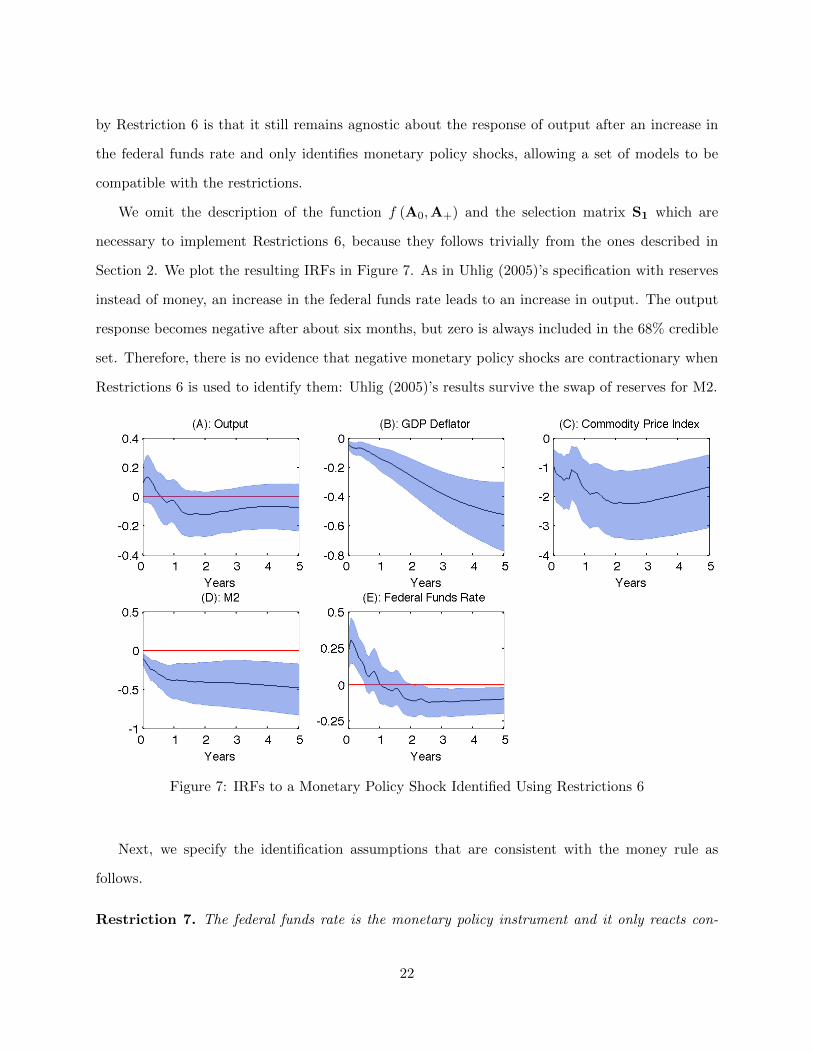
by Restriction 6 is that it still remains agnostic about the response of output after an increase in

the federal funds rate and only identifies monetary policy shocks, allowing a set of models to be

compatible with the restrictions.

We omit the description of the function f (A0,A+) and the selection matrix S1 which are

necessary to implement Restrictions 6, because they follows trivially from the ones described in

Section 2. We plot the resulting IRFs in Figure 7. As in Uhlig (2005)’s specification with reserves

instead of money, an increase in the federal funds rate leads to an increase in output. The output

response becomes negative after about six months, but zero is always included in the 68% credible

set. Therefore, there is no evidence that negative monetary policy shocks are contractionary when

Restrictions 6 is used to identify them: Uhlig (2005)’s results survive the swap of reserves for M2.

Figure 7: IRFs to a Monetary Policy Shock Identified Using Restrictions 6

Next, we specify the identification assumptions that are consistent with the money rule as

follows.

Restriction 7. The federal funds rate is the monetary policy instrument and it only reacts con-

22

temporaneously to money.

Restriction 8. The contemporaneous reaction of the federal funds rate to money is nonnegative.

Here again, we only restrict the behavior of the monetary policy equation while leaving the

remaining equations unrestricted. Therefore, we only identify monetary policy shocks and we

remain agnostic about the response of output after an increase in the federal funds rate. As in the

previous exercises, we do not identify the structural parameters but only set-identify them.

We rewrite the monetary policy equation, concentrating on the contemporaneous coefficients,

as

rt = ψyyt + ψppt + ψpcpc,t + ψmmt + a−10,61ε1,t, (6)

where ψy = a−10,61a0,11, ψp = a−10,61a0,21, ψpc = a−10,61a0,31, and ψm = a−10,61a0,41. Equipped with this

representation of the monetary policy equation, we summarize Restrictions 7 and 8 as follows.

Remark 3. Restriction 7 implies that ψy = ψp = ψpc = 0, while Restriction 8 implies that ψm ≥ 0.

Note also that under Restriction 7, the monetary equation (6) becomes

rt = ψmmt + a−10,61ε1,t. (7)

This equation has three possible interpretations. The first, which is consistent with how we specify

equation (7), is that the federal funds rate responds to changes in the money supply. The second

interpretation is that the money supply adjusts to changes in the federal funds rate. This inter-

pretation is consistent with Sims and Zha’s (2006b) view on how monetary policy was conducted

between 1979 and 1982. A third interpretation is simply that both the federal funds rate and the

money supply respond to Fed actions, and that both indicators are important in describing the

effects of monetary policy on the economy (Belongia and Ireland, 2014). But inference is consistent

with all three different interpretations, which only imply different normalizations in Restriction 8.

In its current form, Restriction 8 states that shocks that raise the money supply lead the Federal

Reserve to increase the federal funds rate. An alternative interpretation is that a monetary policy

23

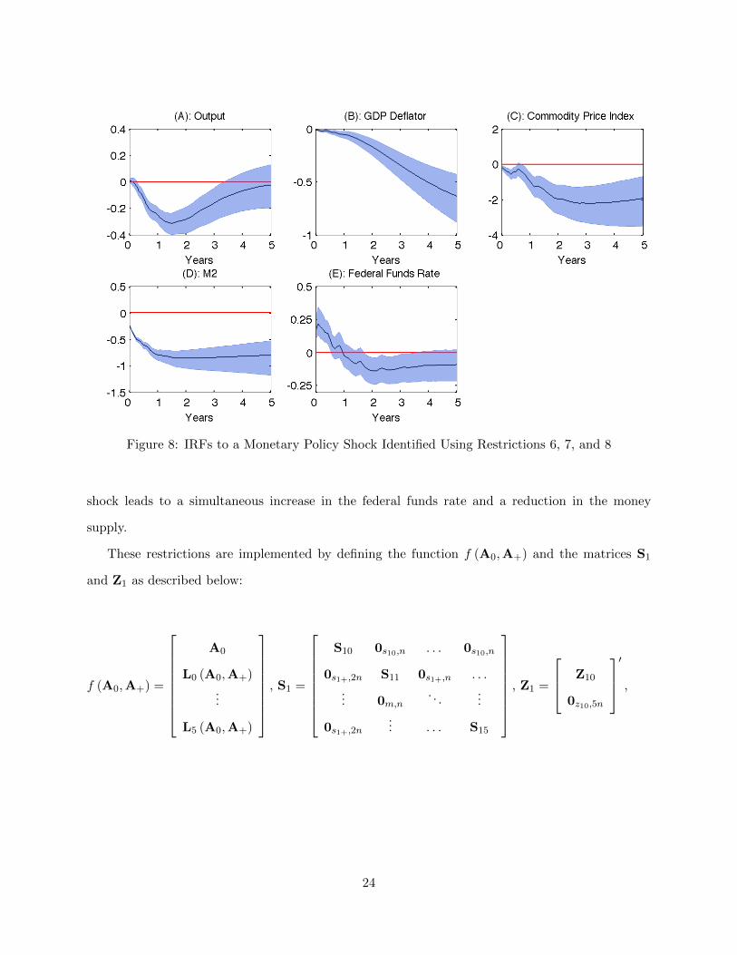
Figure 8: IRFs to a Monetary Policy Shock Identified Using Restrictions 6, 7, and 8

shock leads to a simultaneous increase in the federal funds rate and a reduction in the money

supply.

These restrictions are implemented by defining the function f (A0,A+) and the matrices S1

and Z1 as described below:

f (A0,A+) =

A0

L0 (A0,A+)

...

L5 (A0,A+)

, S1 =

S10 0s10,n . . . 0s10,n

0s1+,2n S11 0s1+,n . . .

... 0m,n. . .

...

0s1+,2n... . . . S15

, Z1 =

Z10

0z10,5n

′

,

24

S10 =

0 0 0 −1 0 01,n

0 0 0 0 1 01,n

0s,1 . . . . . . . . . 0s,1 S

, S =

0 −1 0 0 0

0 0 −1 0 0

0 0 0 −1 0

0 0 0 0 1

,

S1t = S for t = 1, . . . , 5, and Z10 =

1 0 0 0 0 0 0 0 0 0

0 1 0 0 0 0 0 0 0 0

0 0 1 0 0 0 0 0 0 0

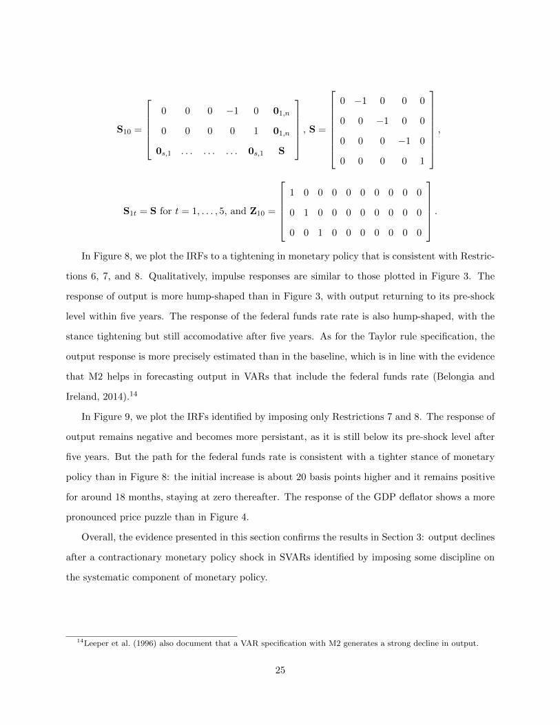
.In Figure 8, we plot the IRFs to a tightening in monetary policy that is consistent with Restric-

tions 6, 7, and 8. Qualitatively, impulse responses are similar to those plotted in Figure 3. The

response of output is more hump-shaped than in Figure 3, with output returning to its pre-shock

level within five years. The response of the federal funds rate rate is also hump-shaped, with the

stance tightening but still accomodative after five years. As for the Taylor rule specification, the

output response is more precisely estimated than in the baseline, which is in line with the evidence

that M2 helps in forecasting output in VARs that include the federal funds rate (Belongia and

Ireland, 2014).14

In Figure 9, we plot the IRFs identified by imposing only Restrictions 7 and 8. The response of

output remains negative and becomes more persistant, as it is still below its pre-shock level after

five years. But the path for the federal funds rate is consistent with a tighter stance of monetary

policy than in Figure 8: the initial increase is about 20 basis points higher and it remains positive

for around 18 months, staying at zero thereafter. The response of the GDP deflator shows a more

pronounced price puzzle than in Figure 4.

Overall, the evidence presented in this section confirms the results in Section 3: output declines

after a contractionary monetary policy shock in SVARs identified by imposing some discipline on

the systematic component of monetary policy.

14Leeper et al. (1996) also document that a VAR specification with M2 generates a strong decline in output.

25

Figure 9: IRFs to a Monetary Policy Shock Identified Using Restrictions 7 and 8

5 Conclusion

The agnostic identification of monetary policy shocks by imposing sign restrictions on IRFs as

proposed by Uhlig (2005) finds that increases in the federal funds rate are not contractionary. We

re-examine this issue and show that the identification scheme in Uhlig (2005) implies a counter-

factual characterization of the systematic component of monetary policy. We design an agnostic

identification scheme that imposes sign and zero restrictions on the systematic component of mone-

tary policy and find that an increase in the federal funds rate leads to a persistent decline in output

and prices.

Overall, our results suggest that while set identification is appealing because it does not require

inference to be based on very specific, and often questionable, exclusion restrictions, it is subject

to the danger of including implausible models. Our suggestion is to impose restrictions on objects

that can be easily evaluated, which in our application is the systematic component of monetary

policy. The issue of how to specify agnostic restrictions in SVARs is not limited to the identifica-

26

tion of monetary policy, and the approach described in this paper can be applied to a variety of

identification problems.

27

References

Arias, J., J. F. Rubio-Ramirez, and D. F. Waggoner (2014): “Inference Based on SVARs

Identified with Sign and Zero Restrictions: Theory and Applications,” International Finance

Discussion Papers (1100). Board of Governors of the Federal Reserve System.

Bagliano, F. C. and C. A. Favero (1998): “Measuring Monetary Policy with VAR Models:

An Evaluation,” European Economic Review, 42, 1069–1112.

Baumeister, C. and L. Benati (2010): “Unconventional Monetary Policy and the Great Reces-

sion,” European Central Bank Working Papers.

Baumeister, C. and J. Hamilton (2014): “Sign Restrictions, Structural Vector Autoregressions,

and Useful Prior Information,” Working Paper.

Beaudry, P., D. Nam, and J. Wang (2011): “Do Mood Swings Drive Business Cycles and is it

Rational?” NBER Working Papers.

Belongia, M. T. and P. N. Ireland (2014): “Interest Rates and Money in the Measurement

of Monetary Policy,” Working Paper 20134, National Bureau of Economic Research.

Bernanke, B. S. and A. S. Blinder (1992): “The Federal Funds Rate and the Channels of

Monetary Transmission,” American Economic Review, 82, 901–21.

Bernanke, B. S. and I. Mihov (1998): “Measuring Monetary Policy,” Quarterly Journal of

Economics, 113, 869–902.

Binning, A. (2013): “Underidentified SVAR Models: A Framework for Combining Short and

Long-run Restrictions with Sign-restrictions,” Norges Bank Working Papers.

Caldara, D. and C. Kamps (2012): “The Analytics of SVARs: A Unified Framework to Measure

Fiscal Multipliers,” Finance and Economics Discussion Series (2012-20). Board of Governors of

the Federal Reserve System.

28

Chappell Jr, H. W., R. R. McGregor, and T. A. Vermilyea (2005): “Committee Decisions

on Monetary Policy: Evidence from Historical Records of the Federal Open Market Committee,”

MIT Press Books, 1.

Christiano, L., M. Eichenbaum, and C. Evans (2005): “Nominal Rigidities and the Dynamic

Effects of a Shock to Monetary Policy,” Journal of Political Economy, 113, 1–45.

Christiano, L. J., M. Eichenbaum, and C. L. Evans (1996): “The Effects of Monetary Policy

Shocks: Evidence from the Flow of Funds,” Review of Economics and Statistics, 16–34.

——— (1999): “Monetary Policy Shocks: What Have we Learned and to What End?” Handbook

of Macroeconomics, 1, 65–148.

Leeper, E. M. and D. B. Gordon (1992): “In Search of the Liquidity Effect,” Journal of

Monetary Economics, 29, 341–369.

Leeper, E. M., C. A. Sims, and T. Zha (1996): “What Does Monetary Policy Do?” Brookings

Papers on Economic Activity, 27, 1–78.

Leeper, E. M. and T. Zha (2003): “Modest Policy Interventions,” Journal of Monetary Eco-

nomics, 50, 1673–1700.

Mountford, A. and H. Uhlig (2009): “What are the Effects of Fiscal Policy Shocks?” Journal

of Applied Econometrics, 24, 960–992.

Peersman, G. and W. B. Wagner (2014): “Shocks to Bank Lending, Risk-Taking, Securitiza-

tion, and Their Role for U.S. Business Cycle Fluctuations,” Discussion Paper 2014-019, Tilburg

University, Center for Economic Research.

Rotemberg, J. and M. Woodford (1997): “An Optimization-based Econometric Framework

for the Evaluation of Monetary Policy,” NBER Macroeconomics Annual 1997, Volume 12, 297–

361.

Rubio-Ramırez, J., D. Waggoner, and T. Zha (2010): “Structural Vector Autoregressions:

Theory of Identification and Algorithms for Inference,” Review of Economic Studies, 77, 665–696.

29

Rudebusch, G. D. (2006): “Monetary Policy Inertia: Fact or Fiction?” International Journal of

Central Banking, 2.

Sims, C. A. (1972): “Money, Income, and Causality,” The American Economic Review, 540–552.

——— (1980): “Macroeconomics and Reality,” Econometrica: Journal of the Econometric Society,

1–48.

——— (1986): “Are Forecasting Models Usable for Policy Analysis?” Federal Reserve Bank of

Minneapolis Quarterly Review, 10, 2–16.

——— (1992): “Interpreting the Macroeconomic Time Series Facts : The Effects of Monetary

Policy,” European Economic Review, 36, 975–1000.

Sims, C. A. and T. Zha (2006a): “Does Monetary Policy Generate Recessions?” Macroeconomic

Dynamics, 10, 231–272.

——— (2006b): “Were There Regime Switches in US Monetary Policy?” American Economic

Review, 54–81.

Taylor, J. B. (1993): “Discretion Versus Policy Rules in Practice,” Carnegie-Rochester Confer-

ence Series on Public Policy, 39, 195–214.

——— (1999): “An Historical Analysis of Monetary Policy Rules,” NBER Working Paper Series,

39.

Uhlig, H. (2005): “What are the Effects of Monetary Policy on Output? Results from an Agnostic

Identification Procedure,” Journal of Monetary Economics, 52, 381–419.

Woodford, M. (2003): “Interest and Prices,” Princeton University Press.

30

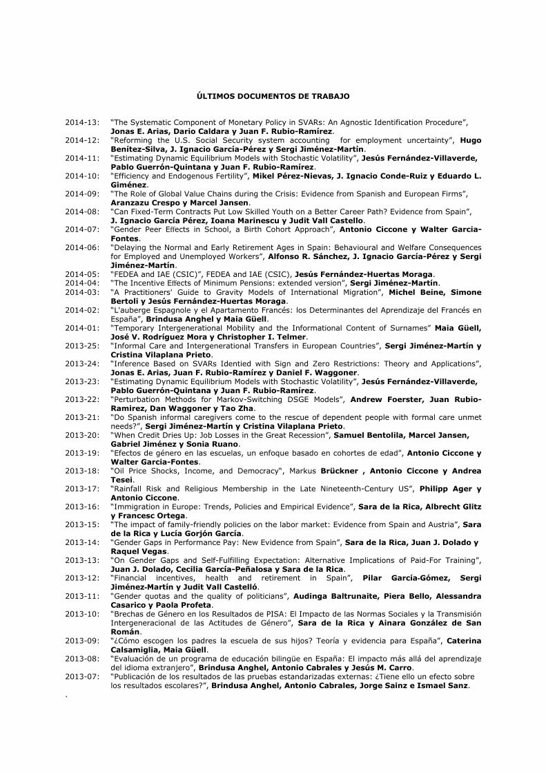
ÚLTIMOS DOCUMENTOS DE TRABAJO

2014-13: “The Systematic Component of Monetary Policy in SVARs: An Agnostic Identification Procedure”,

Jonas E. Arias, Dario Caldara y Juan F. Rubio-Ramírez. 2014-12: “Reforming the U.S. Social Security system accounting for employment uncertainty”, Hugo

Benítez-Silva, J. Ignacio García-Pérez y Sergi Jiménez-Martín. 2014-11: “Estimating Dynamic Equilibrium Models with Stochastic Volatility”, Jesús Fernández-Villaverde,

Pablo Guerrón-Quintana y Juan F. Rubio-Ramírez. 2014-10: “Efficiency and Endogenous Fertility”, Mikel Pérez-Nievas, J. Ignacio Conde-Ruiz y Eduardo L.

Giménez. 2014-09: “The Role of Global Value Chains during the Crisis: Evidence from Spanish and European Firms”,

Aranzazu Crespo y Marcel Jansen. 2014-08: “Can Fixed-Term Contracts Put Low Skilled Youth on a Better Career Path? Evidence from Spain”,

J. Ignacio García Pérez, Ioana Marinescu y Judit Vall Castello. 2014-07: “Gender Peer Effects in School, a Birth Cohort Approach”, Antonio Ciccone y Walter Garcia-

Fontes. 2014-06: “Delaying the Normal and Early Retirement Ages in Spain: Behavioural and Welfare Consequences

for Employed and Unemployed Workers”, Alfonso R. Sánchez, J. Ignacio García-Pérez y Sergi Jiménez-Martín.

2014-05: “FEDEA and IAE (CSIC)”, FEDEA and IAE (CSIC), Jesús Fernández-Huertas Moraga. 2014-04: “The Incentive Effects of Minimum Pensions: extended version”, Sergi Jiménez-Martín. 2014-03: “A Practitioners' Guide to Gravity Models of International Migration”, Michel Beine, Simone

Bertoli y Jesús Fernández-Huertas Moraga. 2014-02: “L'auberge Espagnole y el Apartamento Francés: los Determinantes del Aprendizaje del Francés en

España”, Brindusa Anghel y Maia Güell. 2014-01: “Temporary Intergenerational Mobility and the Informational Content of Surnames” Maia Güell,

José V. Rodríguez Mora y Christopher I. Telmer. 2013-25: “Informal Care and Intergenerational Transfers in European Countries”, Sergi Jiménez-Martín y

Cristina Vilaplana Prieto. 2013-24: “Inference Based on SVARs Identied with Sign and Zero Restrictions: Theory and Applications”,

Jonas E. Arias, Juan F. Rubio-Ramírez y Daniel F. Waggoner. 2013-23: “Estimating Dynamic Equilibrium Models with Stochastic Volatility”, Jesús Fernández-Villaverde,

Pablo Guerrón-Quintana y Juan F. Rubio-Ramírez. 2013-22: “Perturbation Methods for Markov-Switching DSGE Models”, Andrew Foerster, Juan Rubio-

Ramirez, Dan Waggoner y Tao Zha. 2013-21: “Do Spanish informal caregivers come to the rescue of dependent people with formal care unmet

needs?”, Sergi Jiménez-Martín y Cristina Vilaplana Prieto. 2013-20: “When Credit Dries Up: Job Losses in the Great Recession”, Samuel Bentolila, Marcel Jansen,

Gabriel Jiménez y Sonia Ruano. 2013-19: “Efectos de género en las escuelas, un enfoque basado en cohortes de edad”, Antonio Ciccone y

Walter Garcia-Fontes. 2013-18: “Oil Price Shocks, Income, and Democracy“, Markus Brückner , Antonio Ciccone y Andrea

Tesei. 2013-17: “Rainfall Risk and Religious Membership in the Late Nineteenth-Century US”, Philipp Ager y

Antonio Ciccone. 2013-16: “Immigration in Europe: Trends, Policies and Empirical Evidence”, Sara de la Rica, Albrecht Glitz

y Francesc Ortega. 2013-15: “The impact of family-friendly policies on the labor market: Evidence from Spain and Austria”, Sara

de la Rica y Lucía Gorjón García. 2013-14: “Gender Gaps in Performance Pay: New Evidence from Spain”, Sara de la Rica, Juan J. Dolado y

Raquel Vegas. 2013-13: “On Gender Gaps and Self-Fulfilling Expectation: Alternative Implications of Paid-For Training”,

Juan J. Dolado, Cecilia García-Peñalosa y Sara de la Rica. 2013-12: “Financial incentives, health and retirement in Spain”, Pilar García‐‐‐‐Gómez, Sergi

Jiménez‐‐‐‐Martín y Judit Vall Castelló. 2013-11: “Gender quotas and the quality of politicians”, Audinga Baltrunaite, Piera Bello, Alessandra

Casarico y Paola Profeta. 2013-10: “Brechas de Género en los Resultados de PISA: El Impacto de las Normas Sociales y la Transmisión

Intergeneracional de las Actitudes de Género”, Sara de la Rica y Ainara González de San Román.

2013-09: “¿Cómo escogen los padres la escuela de sus hijos? Teoría y evidencia para España”, Caterina Calsamiglia, Maia Güell.

2013-08: “Evaluación de un programa de educación bilingüe en España: El impacto más allá del aprendizaje del idioma extranjero”, Brindusa Anghel, Antonio Cabrales y Jesús M. Carro.

2013-07: “Publicación de los resultados de las pruebas estandarizadas externas: ¿Tiene ello un efecto sobre los resultados escolares?”, Brindusa Anghel, Antonio Cabrales, Jorge Sainz e Ismael Sanz.

.