the tail at store: a revelation from millions of hours of disk … · 3.1 raid architecture raid...
TRANSCRIPT
This paper is included in the Proceedings of the 14th USENIX Conference on
File and Storage Technologies (FAST ’16).February 22–25, 2016 • Santa Clara, CA, USA
ISBN 978-1-931971-28-7
Open access to the Proceedings of the 14th USENIX Conference on
File and Storage Technologies is sponsored by USENIX
The Tail at Store: A Revelation from Millions of Hours of Disk and SSD Deployments
Mingzhe Hao, University of Chicago; Gokul Soundararajan and Deepak Kenchammana-Hosekote, NetApp, Inc.; Andrew A. Chien and Haryadi S. Gunawi, University of Chicago
https://www.usenix.org/conference/fast16/technical-sessions/presentation/hao
USENIX Association 14th USENIX Conference on File and Storage Technologies (FAST ’16) 263
The Tail at Store: A Revelation from
Millions of Hours of Disk and SSD Deployments
Mingzhe Hao†, Gokul Soundararajan∗, Deepak Kenchammana-Hosekote∗,
Andrew A. Chien†, and Haryadi S. Gunawi†
†University of Chicago ∗NetApp, Inc.
Abstract
We study storage performance in over 450,000 disks
and 4,000 SSDs over 87 days for an overall total of 857
million (disk) and 7 million (SSD) drive hours. We find
that storage performance instability is not uncommon:
0.2% of the time, a disk is more than 2x slower than
its peer drives in the same RAID group (and 0.6% for
SSD). As a consequence, disk and SSD-based RAIDs ex-
perience at least one slow drive (i.e., storage tail) 1.5%
and 2.2% of the time. To understand the root causes, we
correlate slowdowns with other metrics (workload I/O
rate and size, drive event, age, and model). Overall,
we find that the primary cause of slowdowns are the in-
ternal characteristics and idiosyncrasies of modern disk
and SSD drives. We observe that storage tails can ad-
versely impact RAID performance, motivating the design
of tail-tolerant RAID. To the best of our knowledge, this
work is the most extensive documentation of storage per-
formance instability in the field.
1 Introduction
Storage, the home of Big Data, has grown enormously
over the past decade [21]. This year Seagate projects to
ship more than 240 exabytes of disk drives [20], SSD
market has doubled in recent years [32], and data stored
in the cloud has also multiplied almost exponentially ev-
ery year [10]. In a world of continuous collection and
analysis of Big Data, storage performance is critical for
many applications. Modern applications particularly de-
mand low and predictable response times, giving rise to
stringent performance SLOs such as “99.9% of all re-
quests must be answered within 300ms” [15, 48]. Per-
formance instability that produces milliseconds of delay
lead to violations of such SLOs, degrading user experi-
ence and impacting revenues negatively [11, 35, 44].
A growing body of literature studies the general prob-
lem of performance instability in large-scale systems,
specifically calling out the impact of stragglers on tail
latencies [7, 13, 14, 34, 45, 50, 52, 54, 56]. Strag-
glers often arise from contention for shared local re-
sources (e.g., CPU, memory) and global resources (e.g.,
network switches, back-end storage), background dae-
mons, scheduling, power limits and energy management,
and many others. These studies are mostly performed at
server, network, or remote (cloud) storage levels.
To date, we find no systematic, large-scale studies of
performance instability in storage devices such as disks
and SSDs. Yet, mounting anecdotal evidence of disk and
SSD performance instability in the field continue to ap-
pear in various forums (§2). Such ad-hoc information is
unable to answer quantitatively key questions about drive
performance instability, questions such as: How much
slowdown do drives exhibit? How often does slowdown
occur? How widespread is it? Does slowdown have tem-
poral behavior? How long can slowdown persist? What
are the potential root causes? What is the impact of tail
latencies from slow drives to the RAID layer? Answers
to these questions could inform a wealth of storage sys-
tems research and design.
To answer these questions, we have performed the
largest empirical analysis of storage performance insta-
bility. Collecting hourly performance logs from cus-
tomer deployments of 458,482 disks and 4,069 SSDs
spanning on average 87 day periods, we have amassed
a dataset that covers 857 million hours of disk and 7 mil-
lion hours of SSD field performance data.
Uniquely, our data includes drive-RAID relationships,
which allows us to compare the performance of each
drive (Di) to that of peer drives in the same RAID group
(i = 1..N ). The RAID and file system architecture in
our study (§3.1) expects that the performance of every
drive (specifically, hourly average latency Li) is similar
to peer drives in the same RAID group.
Our primary metric, drive slowdown ratio (Si), the
fraction of a drive’s latency (Li) over the median latency
of the RAID group (median(L1..N)), captures deviation
from the assumption of homogeneous drive performance.
Assuming that most workloads are balanced across all
the data drives, a normal drive should not be much slower
than the other drives. Therefore, we define “slow” (un-
stable) drive hour when Si ≥ 2 (and “stable” the other-
wise). Throughout the paper, we use 2x and occasionally
1.5x slowdown threshold to classify drives as slow.
264 14th USENIX Conference on File and Storage Technologies (FAST ’16) USENIX Association
In the following segment, we briefly summarize the
findings from our large-scale analysis.
(i) Slowdown occurrences (§4.1.1): Disks and SSDs are
slow (Si ≥ 2) for 0.22% and 0.58% of drive hours in our
study. With a tighter Si ≥ 1.5 threshold, disks and SSDs
are slow for 0.69% and 1.27% of disk hours respectively.
Consequently, stable latencies at 99.9th percentile are
hard to achieve in today’s storage drives. Slowdowns
can also be extreme (i.e., long tails); we observe several
slowdown incidents as large as 2-4 orders of magnitude.
(ii) Tail hours and RAID degradation (§4.1.2): A slow
drive can often make an entire RAID perform poorly.
The observed instability causes RAIDs to suffer 1.5%
and 2.2% of RAID hours with at least one slow drive (i.e.,
“tail hours”). Using 1.5x slowdown threshold, the num-
bers are 4.6% and 4.8%. As a consequent, stable laten-
cies at 99th percentile (or 96th with 1.5x threshold) are
impossible to guarantee in current RAID deployments.
Workload performance (especially full-stripe balanced
workload) will suffer as a consequence of RAID tails.
In our dataset, we observe that RAID throughput can de-
grade during stable to tail hours (§4.4.1).
(iii) Slowdown temporal behavior and extent (§4.1.3,
§4.1.4): We find that slowdown often persists; 40% and
35% of slow disks and SSDs respectively remain unsta-
ble for more than one hour. Slowdown periods exhibit
temporal locality; 90% of disk and 85% of SSD slow-
downs occur on the same day of the previous occurrence.
Finally, slowdown is widespread in the drive population;
our study shows 26% of disks and 29% of SSDs have
experienced at least one slowdown occurrence.
(iv) Workload analysis (§4.2): Drive slowdowns are of-
ten blamed on unbalanced workloads (e.g., a drive is bus-
ier than others). Our findings refute this, showing that
more than 95% of slowdown periods cannot be attributed
to I/O size or rate imbalance.
(v) “The fault is (likely) in our drives”: We find that
older disks exhibit more slowdowns (§4.3.2) and MLC
flash drives exhibit more slowdowns than SLC drives
(§4.3.3). Overall, evidence suggests that most slow-
downs are caused by internal characteristics of modern
disk and SSD drives.
In summary, drive performance instability means the
homogeneous performance assumption of traditional
RAID is no longer accurate. Drive slowdowns can
appear at different times, persist, disappear, and recur
again. Their occurrence is “silent”—not accompanied
by observable drive events (§4.3.1). Most importantly,
workload imbalance is not a major root cause (§4.2).
Replacing slow drives is not a popular solution (§4.4.2-
§4.4.3), mainly because slowdowns are often transient
and drive replacement is expensive in terms of hardware
and RAID rebuild costs.
(vi) The need for tail-tolerant RAID: All of the reasons
above point out that file and RAID systems are now faced
with more responsibilities. Not only must they handle
well-known faults such as latent sector errors and cor-
ruptions, now they must mask storage tail latencies as
well. Therefore, there is an opportunity to create “tail
tolerant” RAID that can mask storage tail latencies on-
line in deployment.
In the following sections, we present further motiva-
tion (§2), our methodology (§3), the main results (§4), an
opportunity assessment of tail-tolerant RAID (§5), dis-
cussion (§6), related work (§7) and conclusion (§8).
2 Motivational Anecdotes
Our work is highly motivated by the mounting anecdotes
of performance instability at the drive level. In the past
several years, we have collected facts and anecdotal ev-
idence of storage “limpware” [16, 26] from literature,
online forums supported by various storage companies,
and conversations with large-scale datacenter operators
as well as product teams. We found many reports of stor-
age performance problems due to various faults, com-
plexities and idiosyncrasies of modern storage devices,
as we briefly summarize below.
Disk: Magnetic disk drives can experience perfor-
mance faults from various root causes such as mechan-
ical wearout (e.g., weak head [1]), sector re-reads due
to media failures such as corruptions and sector er-
rors [2], overheat from broken cooling fans [3], gunk
spilling from actuator assembly and accumulating on
disk head [4], firmware bugs [41], RAID controller de-
fects [16, 47], and vibration from bad disk drive packag-
ing, missing screws, earthquakes, and constant “noise”
in data centers [17, 29]. All these problems can reduce
disk bandwidth by 10-80% and increase latency by sec-
onds. While the problems above can be considered as
performance “faults”, current generation of disks begin
to induce performance instability “by default” (e.g., with
adaptive zoning and Shingled-Magnetic Recording tech-
nologies [5, 18, 33]).
SSD: The pressure to increase flash density translates to
more internal SSD complexities that can induce perfor-
mance instability. For example, SSD garbage collection,
a well-known culprit, can increase latency by a factor
of 100 [13]. Programming MLC cells to different states
(e.g., 0 vs. 3) may require different numbers of itera-
tions due to different voltage thresholds [51]. The notion
of “fast” and “slow” pages exists within an SSD; pro-
gramming a slow page can be 5-8x slower compared to
USENIX Association 14th USENIX Conference on File and Storage Technologies (FAST ’16) 265
Li =
Si = T1
Request latency(full stripe):
10 9 22 118
1 0.9 1.10.82.2T2
D1
RAID
P+Q
ParityDrives
Lmed
DND2 ...D3
T1
I/O
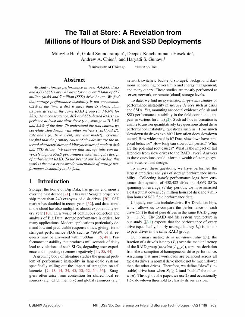
Figure 1: Stable and slow drives in a RAID group.
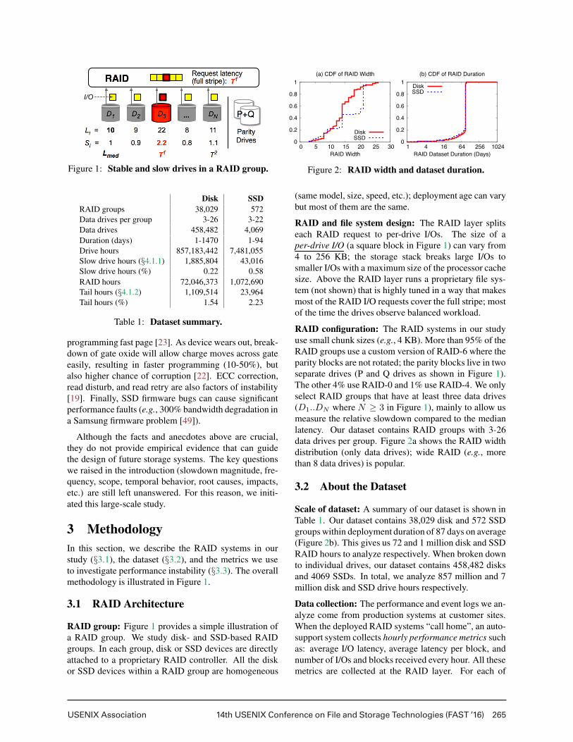
Disk SSD
RAID groups 38,029 572
Data drives per group 3-26 3-22
Data drives 458,482 4,069
Duration (days) 1-1470 1-94
Drive hours 857,183,442 7,481,055
Slow drive hours (§4.1.1) 1,885,804 43,016
Slow drive hours (%) 0.22 0.58
RAID hours 72,046,373 1,072,690
Tail hours (§4.1.2) 1,109,514 23,964
Tail hours (%) 1.54 2.23
Table 1: Dataset summary.
programming fast page [23]. As device wears out, break-
down of gate oxide will allow charge moves across gate
easily, resulting in faster programming (10-50%), but
also higher chance of corruption [22]. ECC correction,
read disturb, and read retry are also factors of instability
[19]. Finally, SSD firmware bugs can cause significant
performance faults (e.g., 300% bandwidth degradation in
a Samsung firmware problem [49]).
Although the facts and anecdotes above are crucial,
they do not provide empirical evidence that can guide
the design of future storage systems. The key questions
we raised in the introduction (slowdown magnitude, fre-
quency, scope, temporal behavior, root causes, impacts,
etc.) are still left unanswered. For this reason, we initi-
ated this large-scale study.
3 Methodology
In this section, we describe the RAID systems in our
study (§3.1), the dataset (§3.2), and the metrics we use
to investigate performance instability (§3.3). The overall
methodology is illustrated in Figure 1.
3.1 RAID Architecture
RAID group: Figure 1 provides a simple illustration of
a RAID group. We study disk- and SSD-based RAID
groups. In each group, disk or SSD devices are directly
attached to a proprietary RAID controller. All the disk
or SSD devices within a RAID group are homogeneous
0
0.2
0.4
0.6
0.8
1
0 5 10 15 20 25 30RAID Width
(a) CDF of RAID Width
DiskSSD 0
0.2
0.4
0.6
0.8
1
1 4 16 64 256 1024RAID Dataset Duration (Days)
(b) CDF of RAID Duration
DiskSSD
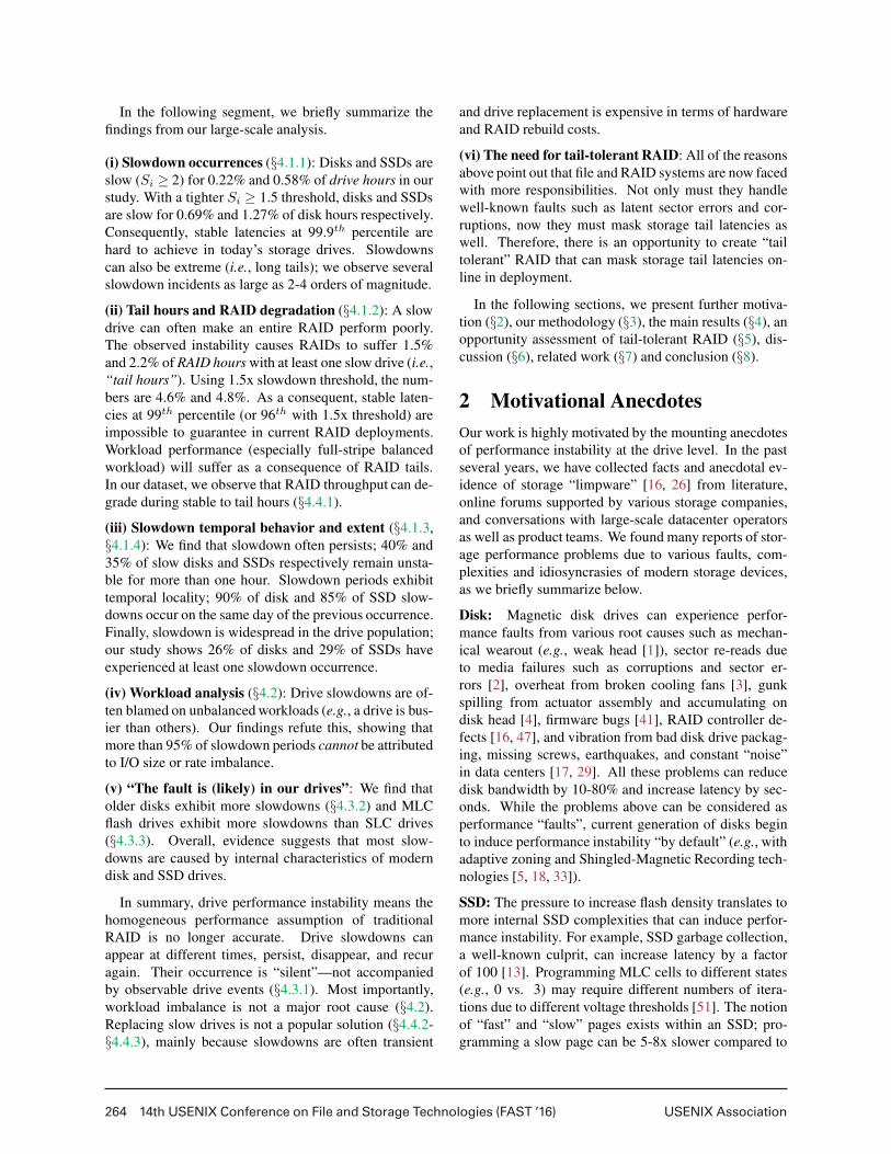
Figure 2: RAID width and dataset duration.
(same model, size, speed, etc.); deployment age can vary
but most of them are the same.
RAID and file system design: The RAID layer splits
each RAID request to per-drive I/Os. The size of a
per-drive I/O (a square block in Figure 1) can vary from
4 to 256 KB; the storage stack breaks large I/Os to
smaller I/Os with a maximum size of the processor cache
size. Above the RAID layer runs a proprietary file sys-
tem (not shown) that is highly tuned in a way that makes
most of the RAID I/O requests cover the full stripe; most
of the time the drives observe balanced workload.
RAID configuration: The RAID systems in our study
use small chunk sizes (e.g., 4 KB). More than 95% of the
RAID groups use a custom version of RAID-6 where the
parity blocks are not rotated; the parity blocks live in two
separate drives (P and Q drives as shown in Figure 1).
The other 4% use RAID-0 and 1% use RAID-4. We only
select RAID groups that have at least three data drives
(D1..DN where N ≥ 3 in Figure 1), mainly to allow us
measure the relative slowdown compared to the median
latency. Our dataset contains RAID groups with 3-26
data drives per group. Figure 2a shows the RAID width
distribution (only data drives); wide RAID (e.g., more
than 8 data drives) is popular.
3.2 About the Dataset
Scale of dataset: A summary of our dataset is shown in
Table 1. Our dataset contains 38,029 disk and 572 SSD
groups within deployment duration of 87 days on average
(Figure 2b). This gives us 72 and 1 million disk and SSD
RAID hours to analyze respectively. When broken down
to individual drives, our dataset contains 458,482 disks
and 4069 SSDs. In total, we analyze 857 million and 7
million disk and SSD drive hours respectively.
Data collection: The performance and event logs we an-
alyze come from production systems at customer sites.
When the deployed RAID systems “call home”, an auto-
support system collects hourly performance metrics such
as: average I/O latency, average latency per block, and
number of I/Os and blocks received every hour. All these
metrics are collected at the RAID layer. For each of
266 14th USENIX Conference on File and Storage Technologies (FAST ’16) USENIX Association
Label Definition
Measured metrics:
N Number of data drives in a RAID group
Di Drive number within a RAID group; i = 1..NLi Hourly average I/O latency observed at Di
Derived metrics:
Lmed Median latency; Lmed = Median of(L1..N )
Si Latency slowdown of Di compared to the median;
Si = Li/Lmed
T k The k-th largest slowdown (“k-th longest tail”);
T 1= Max of (S1..N ),
T 2= 2nd Max of (S1..N ), and so on
Stable A stable drive hour is when Si < 2
Slow A slow drive hour is when Si ≥ 2
Tail A tail hour implies a RAID hour with Ti ≥ 2
Table 2: Primary metrics. The table presents the metrics
used in our analysis. The distribution of N is shown in Figure
2a. Li, Si and T k are explained in Section 3.3.
these metrics, the system separates read and write met-
rics. In addition to performance information, the system
also records drive events such as response timeout, drive
not spinning, unplug/replug events.
3.3 Metrics
Below, we first describe the metrics that are measured
by the RAID systems and recorded in the auto-support
system. Then, we present the metrics that we derived
for measuring tail latencies (slowdowns). Some of the
important metrics are summarized in Table 2.
3.3.1 Measured Metrics
Data drives (N ): This symbol represents the number of
data drives in a RAID group. Our study only includes
data drives mainly because read operations only involve
data drives in our RAID-6 with non-rotating parity. Par-
ity drives can be studied as well, but we leave that for
future work. In terms of write operations, the RAID
small-write problem is negligible due to the file system
optimizations (§3.1).
Per-drive hourly average I/O latency (Li): Of all the
metrics available from the auto-support system, we at
the end only use the hourly average I/O latency (Li) ob-
served by every data drive (Di) in every RAID group
(i=1..N ), as illustrated in Figure 1. We initially ana-
lyzed “throughput” metrics as well, but because the sup-
port system does not record per-IO throughput average,
we cannot make an accurate throughput analysis based
on hourly average I/O sizes and latencies.
Other metrics: We also use other metrics such as per-
drive hourly average I/O rate (Ri) and size (Zi), time
of day, drive age, model, and events (replacements, un-
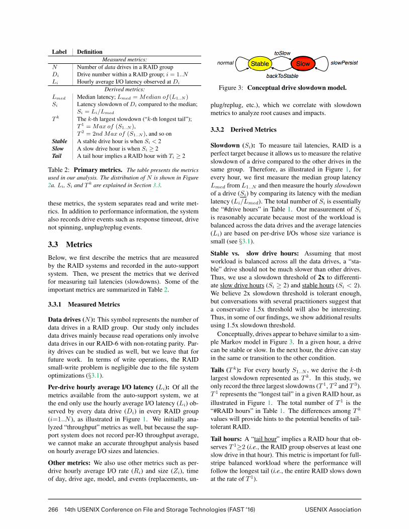
Stable SlowtoSlow
backToStable
slowPersistnormal
Figure 3: Conceptual drive slowdown model.
plug/replug, etc.), which we correlate with slowdown
metrics to analyze root causes and impacts.
3.3.2 Derived Metrics
Slowdown (Si): To measure tail latencies, RAID is a
perfect target because it allows us to measure the relative
slowdown of a drive compared to the other drives in the
same group. Therefore, as illustrated in Figure 1, for
every hour, we first measure the median group latency
Lmed from L1..N and then measure the hourly slowdown
of a drive (Si) by comparing its latency with the median
latency (Li/Lmed). The total number of Si is essentially
the “#drive hours” in Table 1. Our measurement of Si
is reasonably accurate because most of the workload is
balanced across the data drives and the average latencies
(Li) are based on per-drive I/Os whose size variance is
small (see §3.1).
Stable vs. slow drive hours: Assuming that most
workload is balanced across all the data drives, a “sta-
ble” drive should not be much slower than other drives.
Thus, we use a slowdown threshold of 2x to differenti-
ate slow drive hours (Si ≥ 2) and stable hours (Si < 2).
We believe 2x slowdown threshold is tolerant enough,
but conversations with several practitioners suggest that
a conservative 1.5x threshold will also be interesting.
Thus, in some of our findings, we show additional results
using 1.5x slowdown threshold.
Conceptually, drives appear to behave similar to a sim-
ple Markov model in Figure 3. In a given hour, a drive
can be stable or slow. In the next hour, the drive can stay
in the same or transition to the other condition.
Tails (T k): For every hourly S1..N , we derive the k-th
largest slowdown represented as T k. In this study, we
only record the three largest slowdowns (T 1, T 2 and T 3).
T 1 represents the “longest tail” in a given RAID hour, as
illustrated in Figure 1. The total number of T 1 is the
“#RAID hours” in Table 1. The differences among T k
values will provide hints to the potential benefits of tail-
tolerant RAID.
Tail hours: A “tail hour” implies a RAID hour that ob-
serves T 1≥2 (i.e., the RAID group observes at least one
slow drive in that hour). This metric is important for full-
stripe balanced workload where the performance will
follow the longest tail (i.e., the entire RAID slows down
at the rate of T 1).
USENIX Association 14th USENIX Conference on File and Storage Technologies (FAST ’16) 267
0.98
0.985
0.99
0.995
1
1 2 4 8Slowdown Ratio
(a) CDF of Slowdown (Disk)
SiT3T2T1
0.97
0.98
0.99
1
1 2 4 8Slowdown Ratio
(b) CDF of Slowdown (SSD)
SiT3T2T1
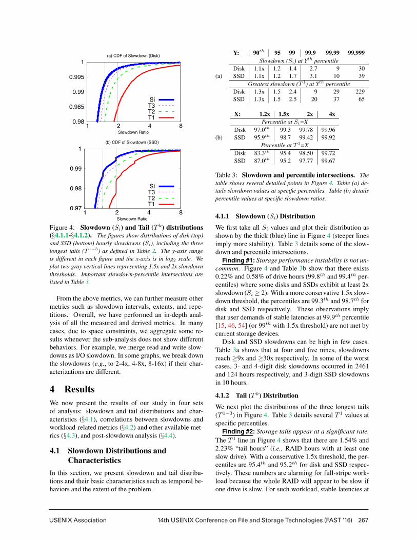
Figure 4: Slowdown (Si) and Tail (T k) distributions
(§4.1.1-§4.1.2). The figures show distributions of disk (top)
and SSD (bottom) hourly slowdowns (Si), including the three
longest tails (T 1−3) as defined in Table 2. The y-axis range
is different in each figure and the x-axis is in log2 scale. We
plot two gray vertical lines representing 1.5x and 2x slowdown
thresholds. Important slowdown-percentile intersections are
listed in Table 3.
From the above metrics, we can further measure other
metrics such as slowdown intervals, extents, and repe-
titions. Overall, we have performed an in-depth anal-
ysis of all the measured and derived metrics. In many
cases, due to space constraints, we aggregate some re-
sults whenever the sub-analysis does not show different
behaviors. For example, we merge read and write slow-
downs as I/O slowdown. In some graphs, we break down
the slowdowns (e.g., to 2-4x, 4-8x, 8-16x) if their char-
acterizations are different.
4 Results
We now present the results of our study in four sets
of analysis: slowdown and tail distributions and char-
acteristics (§4.1), correlations between slowdowns and
workload-related metrics (§4.2) and other available met-
rics (§4.3), and post-slowdown analysis (§4.4).
4.1 Slowdown Distributions and
Characteristics
In this section, we present slowdown and tail distribu-
tions and their basic characteristics such as temporal be-
haviors and the extent of the problem.
(a)
Y: 90th 95 99 99.9 99.99 99.999
Slowdown (Si) at Yth percentile
Disk 1.1x 1.2 1.4 2.7 9 30
SSD 1.1x 1.2 1.7 3.1 10 39
Greatest slowdown (T 1) at Yth percentile
Disk 1.3x 1.5 2.4 9 29 229
SSD 1.3x 1.5 2.5 20 37 65
(b)
X: 1.2x 1.5x 2x 4x
Percentile at Si=X
Disk 97.0th 99.3 99.78 99.96
SSD 95.9th 98.7 99.42 99.92
Percentile at T 1=X
Disk 83.3th 95.4 98.50 99.72
SSD 87.0th 95.2 97.77 99.67
Table 3: Slowdown and percentile intersections. The
table shows several detailed points in Figure 4. Table (a) de-
tails slowdown values at specific percentiles. Table (b) details
percentile values at specific slowdown ratios.
4.1.1 Slowdown (Si) Distribution
We first take all Si values and plot their distribution as
shown by the thick (blue) line in Figure 4 (steeper lines
imply more stability). Table 3 details some of the slow-
down and percentile intersections.
Finding #1: Storage performance instability is not un-
common. Figure 4 and Table 3b show that there exists
0.22% and 0.58% of drive hours (99.8th and 99.4th per-
centiles) where some disks and SSDs exhibit at least 2x
slowdown (Si ≥ 2). With a more conservative 1.5x slow-
down threshold, the percentiles are 99.3th and 98.7th for
disk and SSD respectively. These observations imply
that user demands of stable latencies at 99.9th percentile
[15, 46, 54] (or 99th with 1.5x threshold) are not met by
current storage devices.
Disk and SSD slowdowns can be high in few cases.
Table 3a shows that at four and five nines, slowdowns
reach ≥9x and ≥30x respectively. In some of the worst
cases, 3- and 4-digit disk slowdowns occurred in 2461
and 124 hours respectively, and 3-digit SSD slowdowns
in 10 hours.
4.1.2 Tail (T k) Distribution
We next plot the distributions of the three longest tails
(T 1−3) in Figure 4. Table 3 details several T 1 values at
specific percentiles.
Finding #2: Storage tails appear at a significant rate.
The T 1 line in Figure 4 shows that there are 1.54% and
2.23% “tail hours” (i.e., RAID hours with at least one
slow drive). With a conservative 1.5x threshold, the per-
centiles are 95.4th and 95.2th for disk and SSD respec-
tively. These numbers are alarming for full-stripe work-
load because the whole RAID will appear to be slow if
one drive is slow. For such workload, stable latencies at
268 14th USENIX Conference on File and Storage Technologies (FAST ’16) USENIX Association
0.6
0.7
0.8
0.9
1
2 4 8 16 32 64 128 256Slowdown Interval (Hours)
(a) CDF of Slowdown Interval
DiskSSD 0.5
0.6
0.7
0.8
0.9
1
0 5 10 15 20Inter-Arrival between Slowdowns (Hours)
(b) CDF of Slowdown Inter-Arrival Period
DiskSSD
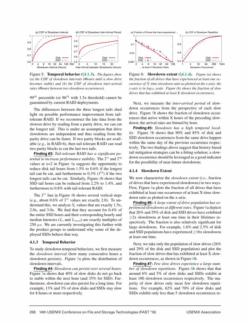
Figure 5: Temporal behavior (§4.1.3). The figures show
(a) the CDF of slowdown intervals (#hours until a slow drive
becomes stable) and (b) the CDF of slowdown inter-arrival
rates (#hours between two slowdown occurrences).
99th percentile (or 96th with 1.5x threshold) cannot be
guaranteed by current RAID deployments.
The differences between the three longest tails shed
light on possible performance improvement from tail-
tolerant RAID. If we reconstruct the late data from the
slowest drive by reading from a parity drive, we can cut
the longest tail. This is under an assumption that drive
slowdowns are independent and thus reading from the
parity drive can be faster. If two parity blocks are avail-
able (e.g., in RAID-6), then tail-tolerant RAID can read
two parity blocks to cut the last two tails.
Finding #3: Tail-tolerant RAID has a significant po-
tential to increase performance stability. The T 1 and T 2
values at x=2 in Figure 4a suggests the opportunity to
reduce disk tail hours from 1.5% to 0.6% if the longest
tail can be cut, and furthermore to 0.3% (T 3) if the two
longest tails can be cut. Similarly, Figure 4b shows that
SSD tail hours can be reduced from 2.2% to 1.4%, and
furthermore to 0.8% with tail-tolerant RAID.
The T 1 line in Figure 4b shows several vertical steps
(e.g., about 0.6% of T 1 values are exactly 2.0). To un-
derstand this, we analyze Si values that are exactly 1.5x,
2.0x, and 3.0x. We find that they account for 0.4% of
the entire SSD hours and their corresponding hourly and
median latencies (Li and Lmed) are exactly multiples of
250 µs. We are currently investigating this further with
the product groups to understand why some of the de-
ployed SSDs behave that way.
4.1.3 Temporal Behavior
To study slowdown temporal behaviors, we first measure
the slowdown interval (how many consecutive hours a
slowdown persists). Figure 5a plots the distribution of
slowdown intervals.
Finding #4: Slowdown can persist over several hours.
Figure 5a shows that 40% of slow disks do not go back
to stable within the next hour (and 35% for SSD). Fur-
thermore, slowdown can also persist for a long time. For
example, 13% and 3% of slow disks and SSDs stay slow
for 8 hours or more respectively.
0.001
0.01
0.1
1
2 4 8 16 32 64 128... at least X Slowdown Ratio
(a) Fraction of Drives that have experienced ...
DiskSSD 0.4
0.6
0.8
1
1 4 16 64 256 1024Slowdown Occurences
(b) CDF of Slowdown Repetition
DiskSSD
Figure 6: Slowdown extent (§4.1.4). Figure (a) shows
the fraction of all drives that have experienced at least one oc-
currence of X-time slowdown ratio as plotted on the x-axis; the
y-axis is in log10 scale. Figure (b) shows the fraction of slow
drives that has exhibited at least X slowdown occurrences.
Next, we measure the inter-arrival period of slow-
down occurrences from the perspective of each slow
drive. Figure 5b shows the fraction of slowdown occur-
rences that arrive within X hours of the preceding slow-
down; the arrival rates are binned by hour.
Finding #5: Slowdown has a high temporal local-
ity. Figure 5b shows that 90% and 85% of disk and
SSD slowdown occurrences from the same drive happen
within the same day of the previous occurrence respec-
tively. The two findings above suggest that history-based
tail mitigation strategies can be a fitting solution; a slow-
down occurrence should be leveraged as a good indicator
for the possibility of near-future slowdowns.
4.1.4 Slowdown Extent
We now characterize the slowdown extent (i.e., fraction
of drives that have experienced slowdowns) in two ways.
First, Figure 6a plots the fraction of all drives that have
exhibited at least one occurrence of at least X-time slow-
down ratio as plotted on the x-axis.
Finding #6: A large extent of drive population has ex-
perienced slowdowns at different rates. Figure 6a depicts
that 26% and 29% of disk and SSD drives have exhibited
≥2x slowdowns at least one time in their lifetimes re-
spectively. The fraction is also relatively significant for
large slowdowns. For example, 1.6% and 2.5% of disk
and SSD populations have experienced≥16x slowdowns
at least one time.
Next, we take only the population of slow drives (26%
and 29% of the disk and SSD population) and plot the
fraction of slow drives that has exhibited at least X slow-
down occurrences, as shown in Figure 6b.
Finding #7: Few slow drives experience a large num-
ber of slowdown repetitions. Figure 6b shows that that
around 6% and 5% of slow disks and SSDs exhibit at
least 100 slowdown occurrences respectively. The ma-
jority of slow drives only incur few slowdown repeti-
tions. For example, 62% and 70% of slow disks and
SSDs exhibit only less than 5 slowdown occurrences re-
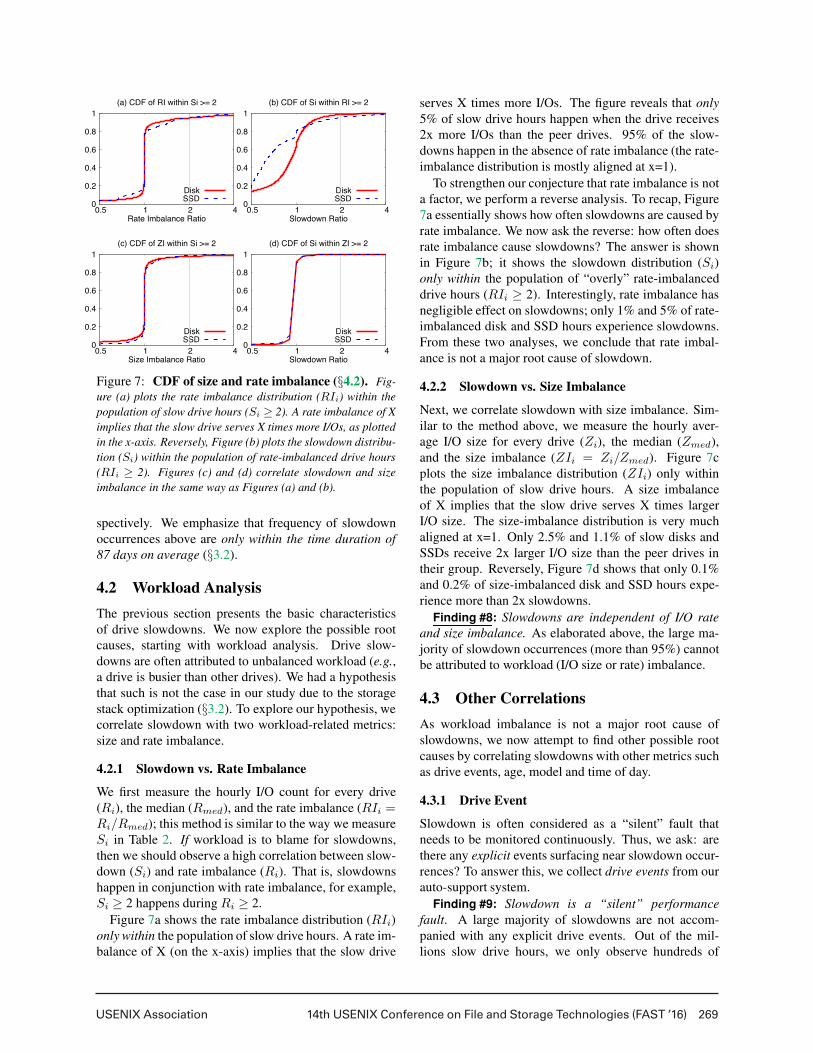
USENIX Association 14th USENIX Conference on File and Storage Technologies (FAST ’16) 269
0
0.2
0.4
0.6
0.8
1
0.5 1 2 4Rate Imbalance Ratio
(a) CDF of RI within Si >= 2
DiskSSD 0
0.2
0.4
0.6
0.8
1
0.5 1 2 4Slowdown Ratio
(b) CDF of Si within RI >= 2
DiskSSD
0
0.2
0.4
0.6
0.8
1
0.5 1 2 4Size Imbalance Ratio
(c) CDF of ZI within Si >= 2
DiskSSD 0
0.2
0.4
0.6
0.8
1
0.5 1 2 4Slowdown Ratio
(d) CDF of Si within ZI >= 2
DiskSSD
Figure 7: CDF of size and rate imbalance (§4.2). Fig-
ure (a) plots the rate imbalance distribution (RIi) within the
population of slow drive hours (Si ≥ 2). A rate imbalance of X
implies that the slow drive serves X times more I/Os, as plotted
in the x-axis. Reversely, Figure (b) plots the slowdown distribu-
tion (Si) within the population of rate-imbalanced drive hours
(RIi ≥ 2). Figures (c) and (d) correlate slowdown and size
imbalance in the same way as Figures (a) and (b).
spectively. We emphasize that frequency of slowdown
occurrences above are only within the time duration of
87 days on average (§3.2).
4.2 Workload Analysis
The previous section presents the basic characteristics
of drive slowdowns. We now explore the possible root
causes, starting with workload analysis. Drive slow-
downs are often attributed to unbalanced workload (e.g.,
a drive is busier than other drives). We had a hypothesis
that such is not the case in our study due to the storage
stack optimization (§3.2). To explore our hypothesis, we
correlate slowdown with two workload-related metrics:
size and rate imbalance.
4.2.1 Slowdown vs. Rate Imbalance
We first measure the hourly I/O count for every drive
(Ri), the median (Rmed), and the rate imbalance (RIi =Ri/Rmed); this method is similar to the way we measure
Si in Table 2. If workload is to blame for slowdowns,
then we should observe a high correlation between slow-
down (Si) and rate imbalance (Ri). That is, slowdowns
happen in conjunction with rate imbalance, for example,
Si ≥ 2 happens during Ri ≥ 2.
Figure 7a shows the rate imbalance distribution (RIi)
only within the population of slow drive hours. A rate im-
balance of X (on the x-axis) implies that the slow drive
serves X times more I/Os. The figure reveals that only
5% of slow drive hours happen when the drive receives
2x more I/Os than the peer drives. 95% of the slow-
downs happen in the absence of rate imbalance (the rate-
imbalance distribution is mostly aligned at x=1).
To strengthen our conjecture that rate imbalance is not
a factor, we perform a reverse analysis. To recap, Figure
7a essentially shows how often slowdowns are caused by
rate imbalance. We now ask the reverse: how often does
rate imbalance cause slowdowns? The answer is shown
in Figure 7b; it shows the slowdown distribution (Si)
only within the population of “overly” rate-imbalanced
drive hours (RIi ≥ 2). Interestingly, rate imbalance has
negligible effect on slowdowns; only 1% and 5% of rate-
imbalanced disk and SSD hours experience slowdowns.
From these two analyses, we conclude that rate imbal-
ance is not a major root cause of slowdown.
4.2.2 Slowdown vs. Size Imbalance
Next, we correlate slowdown with size imbalance. Sim-
ilar to the method above, we measure the hourly aver-
age I/O size for every drive (Zi), the median (Zmed),
and the size imbalance (ZIi = Zi/Zmed). Figure 7c
plots the size imbalance distribution (ZIi) only within
the population of slow drive hours. A size imbalance
of X implies that the slow drive serves X times larger
I/O size. The size-imbalance distribution is very much
aligned at x=1. Only 2.5% and 1.1% of slow disks and
SSDs receive 2x larger I/O size than the peer drives in
their group. Reversely, Figure 7d shows that only 0.1%
and 0.2% of size-imbalanced disk and SSD hours expe-
rience more than 2x slowdowns.
Finding #8: Slowdowns are independent of I/O rate
and size imbalance. As elaborated above, the large ma-
jority of slowdown occurrences (more than 95%) cannot
be attributed to workload (I/O size or rate) imbalance.
4.3 Other Correlations
As workload imbalance is not a major root cause of
slowdowns, we now attempt to find other possible root
causes by correlating slowdowns with other metrics such
as drive events, age, model and time of day.
4.3.1 Drive Event
Slowdown is often considered as a “silent” fault that
needs to be monitored continuously. Thus, we ask: are
there any explicit events surfacing near slowdown occur-
rences? To answer this, we collect drive events from our
auto-support system.
Finding #9: Slowdown is a “silent” performance
fault. A large majority of slowdowns are not accom-
panied with any explicit drive events. Out of the mil-
lions slow drive hours, we only observe hundreds of
270 14th USENIX Conference on File and Storage Technologies (FAST ’16) USENIX Association
0.95
0.96
0.97
0.98
0.99
1
1 2 3 4 5Slowdown Ratio
(a) CDF of Slowdown vs. Drive Age (Disk)
91234576
108 0.99
0.992
0.994
0.996
0.998
1
1 2 3 4Slowdown Ratio
(b) CDF of Slowdown vs. Drive Age (SSD)
3421
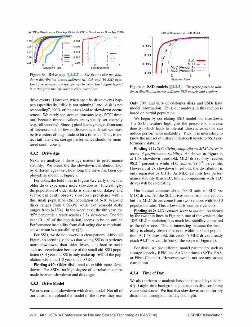
Figure 8: Drive age (§4.3.2). The figures plot the slow-
down distribution across different (a) disk and (b) SSD ages.
Each line represents a specific age by year. Each figure legend
is sorted from the left-most to right-most lines.
drive events. However, when specific drive events hap-
pen (specifically, “disk is not spinning” and “disk is not
responding”), 90% of the cases lead to slowdown occur-
rences. We rarely see storage timeouts (e.g., SCSI time-
out) because timeout values are typically set coarsely
(e.g., 60 seconds). Since typical latency ranges from tens
of microseconds to few milliseconds, a slowdown must
be five orders of magnitude to hit a timeout. Thus, to de-
tect tail latencies, storage performance should be moni-
tored continuously.
4.3.2 Drive Age
Next, we analyze if drive age matters to performance
stability. We break the the slowdown distribution (Si)
by different ages (i.e., how long the drive has been de-
ployed) as shown in Figure 8.
For disks, the bold lines in Figure 8a clearly show that
older disks experience more slowdowns. Interestingly,
the population of older disks is small in our dataset and
yet we can easily observe slowdown prevalence within
this small population (the population of 6-10 year-old
disks ranges from 0.02-3% while 1-5 year-old disks
ranges from 8-33%). In the worst case, the 8th year, the
95th percentile already reaches 2.3x slowdown. The 9th
year (0.11% of the population) seems to be an outlier.
Performance instability from disk aging due to mechani-
cal wear-out is a possibility (§2).
For SSD, we do not observe a clear pattern. Although
Figure 8b seemingly shows that young SSDs experience
more slowdowns than older drives, it is hard to make
such as a conclusion because of the small old-SSD popu-
lation (3-4 year-old SSDs only make up 16% of the pop-
ulation while the 1-2 year-old is 83%).
Finding #10: Older disks tend to exhibit more slow-
downs. For SSDs, no high degree of correlation can be
made between slowdown and drive age.
4.3.3 Drive Model
We now correlate slowdown with drive model. Not all of
our customers upload the model of the drives they use.
0.98
0.985
0.99
0.995
1
1 2 3 4Slowdown Ratio
CDF of Slowdown vs. SSD Model
SLCMLC
MLC (Vendor A)MLC (Vendor B)
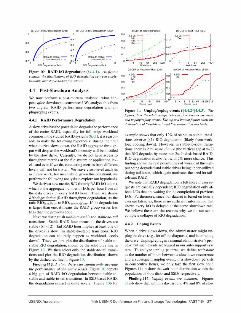
Figure 9: SSD models (§4.3.3). The figure plots the slow-
down distribution across different SSD models and vendors.
Only 70% and 86% of customer disks and SSDs have
model information. Thus, our analysis in this section is
based on partial population.
We begin by correlating SSD model and slowdown.
The SSD literature highlights the pressure to increase
density, which leads to internal idiosyncrasies that can
induce performance instability. Thus, it is interesting to
know the impact of different flash cell levels to SSD per-
formance stability.
Finding #11: SLC slightly outperforms MLC drives in
terms of performance stability. As shown in Figure 9,
at 1.5x slowdown threshold, MLC drives only reaches
98.2th percentile while SLC reaches 99.5th percentile.
However, at 2x slowdown threshold, the distribution is
only separated by 0.1%. As MLC exhibits less perfor-
mance stability than SLC, future comparisons with TLC
drives will be interesting.
Our dataset contains about 60:40 ratio of SLC vs.
MLC drives. All the SLC drives come from one vendor,
but the MLC drives come from two vendors with 90:10
population ratio. This allows us to compare vendors.
Finding #12: SSD vendors seem to matter. As shown
by the two thin lines in Figure 9, one of the vendors (the
10% MLC population) has much less stability compared
to the other one. This is interesting because the insta-
bility is clearly observable even within a small popula-
tion. At 1.5x threshold, this vendor’s MLC drives already
reach 94.3thpercentile (out of the scope of Figure 9).
For disks, we use different model parameters such as
storage capacity, RPM, and SAN interfaces (SATA, SAS,
or Fibre Channel). However, we do not see any strong
correlation.
4.3.4 Time of Day
We also perform an analysis based on time of day to iden-
tify if night-time background jobs such as disk scrubbing
cause slowdowns. We find that slowdowns are uniformly
distributed throughout the day and night.
USENIX Association 14th USENIX Conference on File and Storage Technologies (FAST ’16) 271
0.7
0.8
0.9
1
1 2 4 8RIO Degradation Ratio
(a) CDF of RIO Degradation (Disk)
stable-to-stablestable-to-tail 0.5
0.6
0.7
0.8
0.9
1
1 2 4 8RIO Degradation Ratio
(b) CDF of RIO Degradation (SSD)
stable-to-stablestable-to-tail
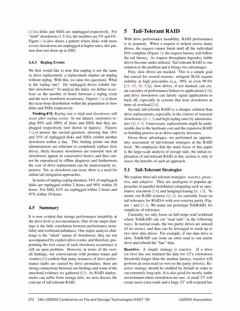
Figure 10: RAID I/O degradation (§4.4.1). The figures
contrast the distributions of RIO degradation between stable-
to-stable and stable-to-tail transitions.
4.4 Post-Slowdown Analysis
We now perform a post-mortem analysis: what hap-
pens after slowdown occurrences? We analyze this from
two angles: RAID performance degradation and un-
plug/replug events.
4.4.1 RAID Performance Degradation
A slow drive has the potential to degrade the performance
of the entire RAID, especially for full-stripe workload
common in the studied RAID systems (§3.1), it is reason-
able to make the following hypothesis: during the hour
when a drive slows down, the RAID aggregate through-
put will drop as the workload’s intensity will be throttled
by the slow drive. Currently, we do not have access to
throughput metrics at the file system or application lev-
els, and even if we do, connecting metrics from different
levels will not be trivial. We leave cross-level analysis
as future work, but meanwhile, given this constraint, we
perform the following analysis to explore our hypothesis.
We derive a new metric, RIO (hourly RAID I/O count),
which is the aggregate number of I/Os per hour from all
the data drives in every RAID hour. Then, we derive
RIO degradation (RAID throughput degradation) as the
ratio RIOlastHour to RIOcurrentHour. If the degradation
is larger than one, it means the RAID group serves less
I/Os than the previous hour.
Next, we distinguish stable-to-stable and stable-to-tail
transitions. Stable RAID hour means all the drives are
stable (Si < 2). Tail RAID hour implies at least one of
the drives is slow. In stable-to-stable transitions, RIO
degradation can naturally happen as workload “cools
down”. Thus, we first plot the distribution of stable-to-
stable RIO degradation, shown by the solid blue line in
Figure 10. We then select only the stable-to-tail transi-
tions and plot the RIO degradation distribution, shown
by the dashed red line in Figure 10.
Finding #13: A slow drive can significantly degrade
the performance of the entire RAID. Figure 10 depicts
a big gap of RAID I/O degradation between stable-to-
stable and stable-to-tail transitions. In SSD-based RAID,
the degradation impact is quite severe. Figure 10b for
0
0.1
0.2
0.3
0.4
1 4 16 64 256 1024Wait-Hour
(a) CDF of Wait-Hour (Disk)
1.5-2x2-4x4-8x8x+
0
0.04
0.08
0.12
1 4 16 64 256 1024Wait-Hour
(b) CDF of Wait-Hour (SSD)
1.5-2x2x+
0
0.2
0.4
0.6
0.8
1 4 16 64 256 1024Recur-Hour
(c) CDF of Recurrent-Hour (Disk)
1.5-2x2-4x4-8x8x+
0
0.2
0.4
0.6
0.8
1 2 4 8 16 32 64 128 256 512Recur-Hour
(d) CDF of Recurrent-Hour (SSD)
1.5-2x2x+
Figure 11: Unplug/replug events (§4.4.2-§4.4.3). The
figures show the relationships between slowdown occurrences
and unplug/replug events. The top and bottom figures show the
distribution of “wait-hour” and “recur-hour” respectively.
example shows that only 12% of stable-to-stable transi-
tions observe ≥2x RIO degradation (likely from work-
load cooling down). However, in stable-to-slow transi-
tions, there is 23% more chance (the vertical gap at x=2)
that RIO degrades by more than 2x. In disk-based RAID,
RIO degradation is also felt with 7% more chance. This
finding shows the real possibilities of workload through-
put being degraded and stable drives being under-utilized
during tail hours, which again motivates the need for tail-
tolerant RAID.
We note that RAID degradation is felt more if user re-
quests are casually dependent; RIO degradation only af-
fects I/Os that are waiting for the completion of previous
I/Os. Furthermore, since our dataset is based on hourly
average latencies, there is no sufficient information that
shows every I/O is delayed at the same slowdown rate.
We believe these are the reasons why we do not see a
complete collapse of RIO degradation.
4.4.2 Unplug Events
When a drive slows down, the administrator might un-
plug the drive (e.g., for offline diagnosis) and later replug
the drive. Unplug/replug is a manual administrator’s pro-
cess, but such events are logged in our auto-support sys-
tem. To analyze unplug patterns, we define wait-hour
as the number of hours between a slowdown occurrence
and a subsequent unplug event; if a slowdown persists
in consecutive hours, we only take the first slow hour.
Figures 11a-b show the wait-hour distribution within the
population of slow disks and SSDs respectively.
Finding #14: Unplug events are common. Figures
11a-b show that within a day, around 4% and 8% of slow
272 14th USENIX Conference on File and Storage Technologies (FAST ’16) USENIX Association
(≥2x) disks and SSDs are unplugged respectively. For
“mild” slowdowns (1.5-2x), the numbers are 3% and 6%.
Figure 11a also shows a pattern where disks with more
severe slowdowns are unplugged at higher rates; this pat-
tern does not show up in SSD.
4.4.3 Replug Events
We first would like to note that unplug is not the same
as drive replacement; a replacement implies an unplug
without replug. With this, we raise two questions: What
is the replug rate? Do replugged drives exhibit fur-
ther slowdowns? To analyze the latter, we define recur-
hour as the number of hours between a replug event
and the next slowdown occurrence. Figures 11c-d show
the recur-hour distribution within the population of slow
disks and SSDs respectively.
Finding #15: Replug rate is high and slowdowns still
recur after replug events. In our dataset, customers re-
plug 89% and 100% of disks and SSDs that they un-
plugged respectively (not shown in figures). Figures
11c-d answer the second question, showing that 18%
and 35% of replugged disks and SSDs exhibit another
slowdown within a day. This finding points out that
administrators are reluctant to completely replace slow
drives, likely because slowdowns are transient (not all
slowdowns appear in consecutive hours) and thus can-
not be reproduced in offline diagnosis and furthermore
the cost of drive replacement can be unnecessarily ex-
pensive. Yet, as slowdown can recur, there is a need for
online tail mitigation approaches.
In terms of unplug-replug duration, 54% of unplugged
disks are replugged within 2 hours and 90% within 10
hours. For SSD, 61% are replugged within 2 hours and
97% within 10 hours.
4.5 Summary
It is now evident that storage performance instability at
the drive level is not uncommon. One of our major find-
ings is the little correlation between performance insta-
bility and workload imbalance. One major analysis chal-
lenge is the “silent” nature of slowdowns; they are not
accompanied by explicit drive events, and therefore, pin-
pointing the root cause of each slowdown occurrence is
still an open problem. However, in terms of the over-
all findings, our conversations with product teams and
vendors [4] confirm that many instances of drive perfor-
mance faults are caused by drive anomalies; there are
strong connections between our findings and some of the
anecdotal evidence we gathered (§2). As RAID deploy-
ments can suffer from storage tails, we next discuss the
concept of tail-tolerant RAID.
5 Tail-Tolerant RAID
With drive performance instability, RAID performance
is in jeopardy. When a request is striped across many
drives, the request cannot finish until all the individual
I/Os complete (Figure 1); the request latency will follow
the tail latency. As request throughput degrades, stable
drives become under-utilized. Tail-tolerant RAID is one
solution to the problem and it brings two advantages.
First, slow drives are masked. This is a simple goal
but crucial for several reasons: stringent SLOs require
stability at high percentiles (e.g., 99% or even 99.9%
[15, 45, 48, 52]); slow drives, if not masked, can cre-
ate cascades of performance failures to applications [16];
and drive slowdowns can falsely signal applications to
back off, especially in systems that treat slowdowns as
hints of overload [24].
Second, tail-tolerant RAID is a cheaper solution than
drive replacements, especially in the context of transient
slowdowns (§4.1.3) and high replug rates by administra-
tors (§4.4.3). Unnecessary replacements might be unde-
sirable due to the hardware cost and the expensive RAID
re-building process as as drive capacity increases.
Given these advantages, we performed an opportu-
nity assessment of tail-tolerant strategies at the RAID
level. We emphasize that the main focus of this paper
is the large-scale analysis of storage tails; the initial ex-
ploration of tail-tolerant RAID in this section is only to
assess the benefits of such an approach.
5.1 Tail-Tolerant Strategies
We explore three tail-tolerant strategies: reactive, proac-
tive, and adaptive. They are analogous to popular ap-
proaches in parallel distributed computing such as spec-
ulative execution [14] and hedging/cloning [6, 13]. To
mimic our RAID systems (§3.2), we currently focus on
tail tolerance for RAID-6 with non-rotating parity (Fig-
ure 1 and §3.1). We name our prototype ToleRAID, for
simplicity of reference.
Currently, we only focus on full-stripe read workload
where ToleRAID can cut “read tails” in the following
ways. In normal reads, the two parity drives are unused
(if no errors), and thus can be leveraged to mask up to
two slow data drives. For example, if one data drive is
slow, ToleRAID can issue an extra read to one parity
drive and rebuild the “late” data.
Reactive: A simple strategy is reactive. If a drive
(or two) has not returned the data for ST x (slowdown
threshold) longer than the median latency, reactive will
perform an extra read (or two) to the parity drive(s). Re-
active strategy should be enabled by default in order to
cut extremely long tails. It is also good for mostly stable
environment where slowdowns are rare. A small ST will
create more extra reads and a large ST will respond late
USENIX Association 14th USENIX Conference on File and Storage Technologies (FAST ’16) 273
to tails. We set ST = 2 in our evaluation, which means
we still need to wait for roughly an additional 1x median
latency to complete the I/O (a total slowdown of 3x in
our case). While reactive strategies work well in clus-
ter computing (e.g., speculative execution for medium-
long jobs), they can react too late for small I/O latencies
(e.g., hundreds of microseconds). Therefore, we explore
proactive and adaptive approaches.
Proactive: This approach performs extra reads to the
parity drives concurrently with the original I/Os. The
number of extra reads can be one (P drive) or two (P
and Q); we name them PROACTIVE1 and PROACTIVE2
respectively. Proactive works well to cut short tails (near
the slowdown threshold); as discussed above, reactive
depends on ST and can be a little bit too late. The down-
side of proactive strategy is the extra read traffic.
Adaptive: This approach is a middle point between the
two strategies above. Adaptive by default runs the re-
active approach. When the reactive policy is triggered
repeatedly for SR times (slowdown repeats) on the same
drive, then ToleRAID becomes proactive until the slow-
down of the offending drive is less than ST . If two
drives are persistently slow, then ToleRAID runs PROAC-
TIVE2. Adaptive is appropriate for instability that comes
from persistent and periodic interferences such as back-
ground SSD GC, SMR log cleaning, or I/O contention
from multi-tenancy.
5.2 Evaluation
Our user-level ToleRAID prototype stripes each RAID
request into 4-KB chunks (§3.2), merge consecutive per-
drive chunks, and submit them as direct I/Os. We in-
sert a delay-injection layer that emulates I/O slowdowns.
Our prototype takes two inputs: block-level trace and
slowdown distribution. Below, we show ToleRAID re-
sults from running a block trace from Hadoop Word-
count benchmark, which contains mostly big reads. We
perform the experiments on 8-drive RAID running IBM
500GB SATA-600 7.2K disk drives.
We use two slowdown distributions: (1) Rare distribu-
tion, which is uniformly sampled from our disk dataset
(Figure 4a). Here, tails (T 1) are rare (1.5%) but long tails
exist (Table 3). (2) Periodic distribution, based on our
study of Amazon EC2 ephemeral SSDs (not shown due
to space constraints). In this study, we rent SSD nodes
and found a case where one of the locally-attached SSDs
periodically exhibited 5x read slowdowns that lasted for
3-6 minutes and repeated every 2-3 hours (2.3% instabil-
ity period on average).
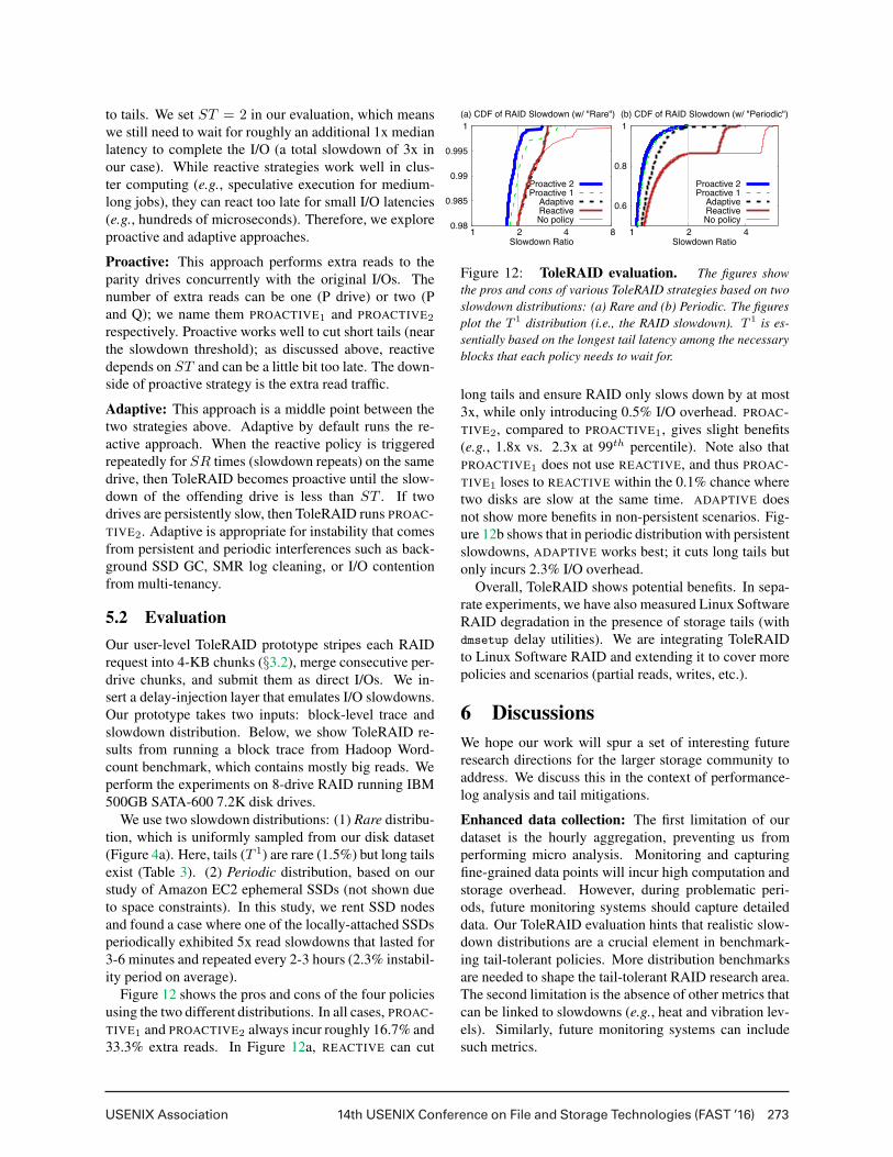
Figure 12 shows the pros and cons of the four policies
using the two different distributions. In all cases, PROAC-
TIVE1 and PROACTIVE2 always incur roughly 16.7% and
33.3% extra reads. In Figure 12a, REACTIVE can cut
0.98
0.985
0.99
0.995
1
1 2 4 8Slowdown Ratio
(a) CDF of RAID Slowdown (w/ "Rare")
Proactive 2Proactive 1
AdaptiveReactiveNo policy
0.6
0.8
1
1 2 4Slowdown Ratio
(b) CDF of RAID Slowdown (w/ "Periodic")
Proactive 2Proactive 1
AdaptiveReactiveNo policy
Figure 12: ToleRAID evaluation. The figures show
the pros and cons of various ToleRAID strategies based on two
slowdown distributions: (a) Rare and (b) Periodic. The figures
plot the T 1 distribution (i.e., the RAID slowdown). T 1 is es-
sentially based on the longest tail latency among the necessary
blocks that each policy needs to wait for.
long tails and ensure RAID only slows down by at most
3x, while only introducing 0.5% I/O overhead. PROAC-
TIVE2, compared to PROACTIVE1, gives slight benefits
(e.g., 1.8x vs. 2.3x at 99th percentile). Note also that
PROACTIVE1 does not use REACTIVE, and thus PROAC-
TIVE1 loses to REACTIVE within the 0.1% chance where
two disks are slow at the same time. ADAPTIVE does
not show more benefits in non-persistent scenarios. Fig-
ure 12b shows that in periodic distribution with persistent
slowdowns, ADAPTIVE works best; it cuts long tails but
only incurs 2.3% I/O overhead.
Overall, ToleRAID shows potential benefits. In sepa-
rate experiments, we have also measured Linux Software
RAID degradation in the presence of storage tails (with
dmsetup delay utilities). We are integrating ToleRAID
to Linux Software RAID and extending it to cover more
policies and scenarios (partial reads, writes, etc.).
6 Discussions
We hope our work will spur a set of interesting future
research directions for the larger storage community to
address. We discuss this in the context of performance-
log analysis and tail mitigations.
Enhanced data collection: The first limitation of our
dataset is the hourly aggregation, preventing us from
performing micro analysis. Monitoring and capturing
fine-grained data points will incur high computation and
storage overhead. However, during problematic peri-
ods, future monitoring systems should capture detailed
data. Our ToleRAID evaluation hints that realistic slow-
down distributions are a crucial element in benchmark-
ing tail-tolerant policies. More distribution benchmarks
are needed to shape the tail-tolerant RAID research area.
The second limitation is the absence of other metrics that
can be linked to slowdowns (e.g., heat and vibration lev-
els). Similarly, future monitoring systems can include
such metrics.

274 14th USENIX Conference on File and Storage Technologies (FAST ’16) USENIX Association
Our current SSD dataset is two orders of magnitude
smaller than the disk dataset. As SSD becomes the
front-end storage in datacenters, larger and longer stud-
ies of SSD performance instability is needed. Similarly,
denser SMR disk drives will replace old generation disks
[5, 18]. Performance studies of SSD-based and SMR-
based RAID will be valuable, especially for understand-
ing the ramifications of internal SSD garbage-collection
and SMR cleaning to the overall RAID performance.
Further analyses: Correlating slowdowns to latent sec-
tor errors, corruptions, drive failures (e.g., from SMART
logs), and application performance would be interesting
future work. One challenge we had was that not all ven-
dors consistently use SMART and report drive errors. In
this paper, we use median values to measure tail laten-
cies and slowdowns similar to other work [13, 34, 52].
We do so because using median values will not hide the
severity of long tails. Using median is exaggerating if
(N-1)/2 of the drives have significantly higher latencies
than the rest; however, we did not observe such cases.
Finally, we mainly use 2x slowdown threshold, and oc-
casionally show results from a more conservative 1.5x
threshold. Further analyses based on average latency val-
ues and different threshold levels are possible.
Tail mitigations: We believe the design space of tail-
tolerant RAID is vast considering different forms of
RAID (RAID-5/6/10, etc.), different types of erasure
coding [38], various slowdown distributions in the field,
and diverse user SLA expectations. In our initial assess-
ment, ToleRAID uses a black-box approach, but there
are other opportunities to cut tails “at the source” with
transparent interactions between devices and the RAID
layer. In special cases such as materials trapped between
disk head and platter (which will be more prevalent in
“slim” drives with low heights), the file system or RAID
layer can inject random I/Os to “sweep” the dust off. In
summary, each root cause can be mitigated with specific
strategies. The process of identifying all possible root
causes of performance instability should be continued for
future mitigation designs.
7 Related Work
Large-scale storage studies at the same scale as ours were
conducted for analysis of whole-disk failures [37, 40],
latent sector errors [8, 36], and sector corruptions [9].
Many of these studies were started based on anecdotal
evidence of storage faults. Today, as these studies had
provided real empirical evidence, it is a common expec-
tation that storage devices exhibit such faults. Likewise,
our study will provide the same significance of contribu-
tion, but in the context of performance faults.
Krevat et al. [33] demonstrate that disks are like
“snowflakes” (same model can have 5-14% throughput
variance); they only analyze throughput metrics on 70
drives with simple microbenchmarks. To the best of our
knowledge, our work is the first to conduct a large-scale
performance instability analysis at the drive level.
Storage performance variability is typically addressed
in the context of storage QoS (e.g., mClock [25], PARDA
[24], Pisces [42]) and more recently in cloud storage ser-
vices (e.g., C3 [45], CosTLO [52]). Other recent work
reduces performance variability at the file system (e.g.,
Chopper [30]), I/O scheduler (e.g., split-level schedul-
ing [55]), and SSD layers (e.g., Purity [12], Flash on
Rails [43]). Different than ours, these sets of work do
not specifically target drive-level tail latencies.
Finally, as mentioned before, reactive, proactive and
adaptive tail-tolerant strategies are lessons learned from
the distributed cluster computing (e.g., MapReduce [14],
dolly [6], Mantri [7], KMN [50]) and distributed storage
systems (e.g., Windows Azure Storage [31], RobuSTore
[53]). The applications of these high-level strategies in
the context of RAID will significantly differ.
8 Conclusion
We have “transformed” anecdotes of storage perfor-
mance instability into large-scale empirical evidence.
Our analysis so far is solely based on last generation
drives (few years in deployment). With trends in disk and
SSD technology (e.g., SMR disks, TLC flash devices),
the worst might be yet to come; performance instability
can be more prevalent in the future, and our findings are
perhaps just the beginning. File and RAID systems are
now faced with more responsibilities. Not only must they
handle known storage faults such as latent sector errors
and corruptions [9, 27, 28, 39], but also now they must
mask drive tail latencies as well. Lessons can be learned
from the distributed computing community where a large
body of work has been born since the issue of tail laten-
cies became a spotlight a decade ago [14]. Similarly, we
hope “the tail at store” will spur exciting new research
directions within the storage community.
9 Acknowledgments
We thank Bianca Schroeder, our shepherd, and the
anonymous reviewers for their tremendous feedback and
comments. We also would like to thank Lakshmi N.
Bairavasundaram and Shiqin Yan for their initial help
and Siva Jayasenan and Art Harkin for their managerial
support. This material is based upon work supported by
NetApp, Inc. and the NSF (grant Nos. CCF-1336580,
CNS-1350499 and CNS-1526304).
USENIX Association 14th USENIX Conference on File and Storage Technologies (FAST ’16) 275
References[1] Weak Head. http://forum.hddguru.com/search.
php?keywords=weak-head.
[2] Personal Communication from Andrew Baptist ofCleversafe, 2013.
[3] Personal Communication from Garth Gibson of CMU,2013.
[4] Personal Communication from NetApp Hardware andProduct Teams, 2015.
[5] Abutalib Aghayev and Peter Desnoyers. Skylight-AWindow on Shingled Disk Operation. In Proceedings ofthe 13th USENIX Symposium on File and StorageTechnologies (FAST), 2015.
[6] Ganesh Ananthanarayanan, Ali Ghodsi, Scott Shenker,and Ion Stoica. Effective Straggler Mitigation: Attack ofthe Clones. In Proceedings of the 10th Symposium onNetworked Systems Design and Implementation (NSDI),2013.
[7] Ganesh Ananthanarayanan, Srikanth Kandula, AlbertGreenberg, Ion Stoica, Yi Lu, Bikas Saha, and EdwardHarris. Reining in the Outliers in Map-Reduce Clustersusing Mantri. In Proceedings of the 9th Symposium onOperating Systems Design and Implementation (OSDI),2010.
[8] Lakshmi N. Bairavasundaram, Garth R. Goodson,Shankar Pasupathy, and Jiri Schindler. An Analysis ofLatent Sector Errors in Disk Drives. In Proceedings ofthe 2007 ACM Conference on Measurement andModeling of Computer Systems (SIGMETRICS), 2007.
[9] Lakshmi N. Bairavasundaram, Garth R. Goodson,Bianca Schroeder, Andrea C. Arpaci-Dusseau, andRemzi H. Arpaci-Dusseau. An Analysis of DataCorruption in the Storage Stack. In Proceedings of the6th USENIX Symposium on File and StorageTechnologies (FAST), 2008.
[10] Jeff Barr. Amazon S3 - 905 Billion Objects and 650,000Requests/Second. http://aws.amazon.com/cn/blogs/aws/amazon-s3-905-billion-objects-and-650000-requestssecond, 2012.
[11] Jake Brutlag. Speed Matters for Google Web Search.http://services.google.com/fh/files/blogs/google_delayexp.pdf, 2009.
[12] John Colgrove, John D. Davis, John Hayes, Ethan L.Miller, Cary Sandvig, Russell Sears, Ari Tamches, NeilVachharajani, and Feng Wang. Purity: Building fast,highly-available enterprise flash storage fromcommodity components. In Proceedings of the 2015ACM SIGMOD International Conference onManagement of Data (SIGMOD), 2015.
[13] Jeffrey Dean and Luiz Andr Barroso. The Tail at Scale.Communications of the ACM, 56(2), February 2013.
[14] Jeffrey Dean and Sanjay Ghemawat. MapReduce:Simplified Data Processing on Large Clusters. InProceedings of the 6th Symposium on Operating SystemsDesign and Implementation (OSDI), 2004.
[15] Giuseppe DeCandia, Deniz Hastorun, Madan Jampani,Gunavardhan Kakulapati, Avinash Lakshman, AlexPilchin, Swaminathan Sivasubramanian, Peter Vosshall,and Werner Vogels. Dynamo: Amazon’s HighlyAvailable Key-value Store. In Proceedings of the 21stACM Symposium on Operating Systems Principles(SOSP), 2007.
[16] Thanh Do, Mingzhe Hao, Tanakorn Leesatapornwongsa,Tiratat Patana-anake, and Haryadi S. Gunawi. Limplock:
Understanding the Impact of Limpware on Scale-OutCloud Systems. In Proceedings of the 4th ACMSymposium on Cloud Computing (SoCC), 2013.
[17] Michael Feldman. Startup Takes Aim atPerformance-Killing Vibration in Datacenter. http://www.hpcwire.com/2010/01/19/startuptakes aim at performance-killingvibration in datacenter/, 2010.
[18] Tim Feldman and Garth Gibson. Shingled MagneticRecording: Areal Density Increase Requires New DataManagement. USENIX ;login: Magazine, 38(3), Jun2013.
[19] Robert Frickey. Data Integrity on 20nm SSDs. In FlashMemory Summit, 2012.
[20] Natalie Gagliordi. Seagate Q2 solid, 61.3 exabytesshipped. http://www.zdnet.com/article/seagate-q2-solid-61-3-exabytes-shipped/,2015.
[21] John Gantz and David Reinsel. The digital universe in2020. http://www.emc.com/collateral/analyst-reports/idc-the-digital-universe-in-2020.pdf, 2012.
[22] Laura M. Grupp, Adrian M. Caulfield, Joel Coburn,Steven Swanson, Eitan Yaakobi, Paul H. Siegel, andJack K. Wolf. Characterizing flash memory: anomalies,observations, and applications. In 42nd AnnualIEEE/ACM International Symposium onMicroarchitecture (MICRO-42), 2009.
[23] Laura M. Grupp, John D. Davis, and Steven Swanson.The Bleak Future of NAND Flash Memory. InProceedings of the 10th USENIX Symposium on File andStorage Technologies (FAST), 2012.
[24] Ajay Gulati, Irfan Ahmad, and Carl A. Waldspurger.PARDA: Proportional Allocation of Resources forDistributed Storage Access. In Proceedings of the 7thUSENIX Symposium on File and Storage Technologies(FAST), 2009.
[25] Ajay Gulati, Arif Merchant, and Peter J. Varman.mClock: Handling Throughput Variability forHypervisor IO Scheduling. In Proceedings of the 9thSymposium on Operating Systems Design andImplementation (OSDI), 2010.
[26] Haryadi S. Gunawi, Mingzhe Hao, TanakornLeesatapornwongsa, Tiratat Patana-anake, Thanh Do,Jeffry Adityatama, Kurnia J. Eliazar, Agung Laksono,Jeffrey F. Lukman, Vincentius Martin, and Anang D.Satria. What Bugs Live in the Cloud? A Study of 3000+Issues in Cloud Systems. In Proceedings of the 5th ACMSymposium on Cloud Computing (SoCC), 2014.
[27] Haryadi S. Gunawi, Vijayan Prabhakaran, SwethaKrishnan, Andrea C. Arpaci-Dusseau, and Remzi H.Arpaci-Dusseau. Improving File System Reliability withI/O Shepherding. In Proceedings of the 21st ACMSymposium on Operating Systems Principles (SOSP),2007.
[28] Haryadi S. Gunawi, Abhishek Rajimwale, Andrea C.Arpaci-Dusseau, and Remzi H. Arpaci-Dusseau. SQCK:A Declarative File System Checker. In Proceedings ofthe 8th Symposium on Operating Systems Design andImplementation (OSDI), 2008.
[29] Robin Harris. Bad, bad, bad vibrations. http://www.zdnet.com/article/bad-bad-bad-vibrations/,2010.
[30] Jun He, Duy Nguyen, Andrea C. Arpaci-Dusseau, andRemzi H. Arpaci-Dusseau. Reducing File System Tail
276 14th USENIX Conference on File and Storage Technologies (FAST ’16) USENIX Association
Latencies with Chopper. In Proceedings of the 13thUSENIX Symposium on File and Storage Technologies(FAST), 2015.
[31] Cheng Huang, Huseyin Simitci, Yikang Xu, AaronOgus, Brad Calder, Parikshit Gopalan, Jin Li, and SergeyYekhanin. Erasure Coding in Windows Azure Storage.In Proceedings of the 2012 USENIX Annual TechnicalConference (ATC), 2012.
[32] Jennifer Johnson. SSD Market On Track For More ThanDouble Growth This Year. http://hothardware.com/news/SSD-Market-On-Track-For-More-Than-Double-Growth-This-Year, 2013.
[33] Elie Krevat, Joseph Tucek, and Gregory R. Ganger.Disks Are Like Snowflakes: No Two Are Alike. In The13th Workshop on Hot Topics in Operating Systems(HotOS XIII), 2011.
[34] Jialin Li, Naveen Kr. Sharma, Dan R. K. Ports, andSteven D. Gribble. Tales of the Tail: Hardware, OS, andApplication-level Sources of Tail Latency. InProceedings of the 5th ACM Symposium on CloudComputing (SoCC), 2014.
[35] Jim Liddle. Amazon found every 100ms of latency costthem 1% in sales. http://blog.gigaspaces.com/amazon-found-every-100ms-of-latency-cost-them-1-in-sales/, 2008.
[36] Ao Ma, Fred Douglis, Guanlin Lu, Darren Sawyer,Surendar Chandra, and Windsor Hsu. RAIDShield:Characterizing, Monitoring, and Proactively ProtectingAgainst Disk Failures. In Proceedings of the 13thUSENIX Symposium on File and Storage Technologies(FAST), 2015.
[37] Eduardo Pinheiro, Wolf-Dietrich Weber, and Luiz AndreBarroso. Failure Trends in a Large Disk DrivePopulation. In Proceedings of the 5th USENIXSymposium on File and Storage Technologies (FAST),2007.
[38] James S. Plank, Jianqiang Luo, Catherine D. Schuman,Lihao Xu, and Zooko Wilcox-O’Hearn. A PerformanceEvaluation and Examination of Open-Source ErasureCoding Libraries for Storage. In Proceedings of the 7thUSENIX Symposium on File and Storage Technologies(FAST), 2009.
[39] Bianca Schroeder, Sotirios Damouras, and Phillipa Gill.Understanding Latent Sector Errors and How to ProtectAgainst Them. In Proceedings of the 8th USENIXSymposium on File and Storage Technologies (FAST),2010.
[40] Bianca Schroeder and Garth A. Gibson. Disk failures inthe real world: What does an MTTF of 1,000,000 hoursmean to you? In Proceedings of the 5th USENIXSymposium on File and Storage Technologies (FAST),2007.
[41] Anand Lal Shimpi. Intel Discovers Bug in 6-SeriesChipset: Our Analysis. http://www.anandtech.com/show/4142/intel-discovers-bug-in-6series-chipset-begins-recall, 2011.
[42] David Shue, Michael J. Freedman, and Anees Shaikh.Performance Isolation and Fairness for Multi-TenantCloud Storage. In Proceedings of the 10th Symposiumon Operating Systems Design and Implementation(OSDI), 2012.
[43] Dimitris Skourtis, Dimitris Achlioptas, Noah Watkins,Carlos Maltzahn, and Scott Brandt. Flash on rails:Consistent flash performance through redundancy. InProceedings of the 2014 USENIX Annual TechnicalConference (ATC), 2014.
[44] Steve Souders. Velocity and the Bottom Line. http://radar.oreilly.com/2009/07/velocity-making-your-site-fast.html, 2009.
[45] Lalith Suresh, Marco Canini, Stefan Schmid, and AnjaFeldmann. C3: Cutting Tail Latency in Cloud DataStores via Adaptive Replica Selection. In Proceedings ofthe 12th Symposium on Networked Systems Design andImplementation (NSDI), 2015.
[46] Lalith Suresh, Marco Canini, Stefan Schmid, and AnjaFeldmann. C3: Cutting Tail Latency in Cloud DataStores via Adaptive Replica Selection. In Proceedings ofthe 12th Symposium on Networked Systems Design andImplementation (NSDI), 2015.
[47] Utah Emulab Testbed. RAID controller timeoutproblems on boss node, on 6/21/2013. http://www.emulab.net/news.php3, 2013.
[48] Beth Trushkowsky, Peter Bodik, Armando Fox,Michael J. Franklin, Michael I. Jordan, and David A.Patterson. The SCADS Director: Scaling a DistributedStorage System Under Stringent PerformanceRequirements. In Proceedings of the 9th USENIXSymposium on File and Storage Technologies (FAST),2011.
[49] Kristian Vatto. Samsung Acknowledges the SSD 840EVO Read Performance Bug - Fix Is on the Way.http://www.anandtech.com/show/8550/samsung-acknowledges-the-ssd-840-evo-read-performance-bug-fix-is-on-the-way, 2014.
[50] Shivaram Venkataraman, Aurojit Panda, GaneshAnanthanarayanan, Michael J. Franklin, and Ion Stoica.The Power of Choice in Data-Aware Cluster Scheduling.In Proceedings of the 11th Symposium on OperatingSystems Design and Implementation (OSDI), 2014.
[51] Guanying Wu and Xubin He. Reducing SSD ReadLatency via NAND Flash Program and EraseSuspension. In Proceedings of the 10th USENIXSymposium on File and Storage Technologies (FAST),2012.
[52] Zhe Wu, Curtis Yu, and Harsha V. Madhyastha.CosTLO: Cost-Effective Redundancy for Lower LatencyVariance on Cloud Storage Services. In Proceedings ofthe 12th Symposium on Networked Systems Design andImplementation (NSDI), 2015.
[53] Huaxia Xia and Andrew A. Chien. RobuSTore: RobustPerformance for Distributed Storage Systems. InProceedings of the 2007 Conference on HighPerformance Networking and Computing (SC), 2007.
[54] Neeraja J. Yadwadkar, Ganesh Ananthanarayanan, andRandy Katz. Wrangler: Predictable and Faster Jobsusing Fewer Resources. In Proceedings of the 5th ACMSymposium on Cloud Computing (SoCC), 2014.
[55] Suli Yang, Tyler Harter, Nishant Agrawal, Salini SelvarajKowsalya, Anand Krishnamurthy, Samer Al-Kiswany,Rini T. Kaushik, Andrea C. Arpaci-Dusseau, andRemzi H. Arpaci-Dusseau. Split-Level I/O Scheduling.In Proceedings of the 25th ACM Symposium onOperating Systems Principles (SOSP), 2015.
[56] Matei Zaharia, Andy Konwinski, Anthony D. Joseph,Randy Katz, and Ion Stoica. Improving MapReducePerformance in Heterogeneous Environments. InProceedings of the 8th Symposium on Operating SystemsDesign and Implementation (OSDI), 2008.