the technique of early determination of reservoir drive of...

TWMS J. Pure Appl. Math., V.8, N.2, 2017, pp.236-250

THE TECHNIQUE OF EARLY DETERMINATION OF RESERVOIR DRIVE

OF GAS CONDENSATE AND VELOTAIL OIL DEPOSITS ON THE BASIS

OF NEW DIAGNOSIS INDICATORS

M.A. JAMALBAYOV1, N.A. VELIYEV2

Abstract. The purpose of this study is to find new indicators to characterize the drive mech-

anism and develop a method for early determination of reservoir drive. The results of our

investigation showed that there is a strict relationship between the reservoir drive and the rela-

tions of pore volume to reservoir pressure and porosity. New diagnosis indicators to help identify

the drive mechanism called Reservoir Drive Performance Indexes (RDPI) have been found. A

technique based on RDPI for early determination and characterization of the drive mechanism

of gas-condensate, volatile and black-oil reservoirs has been developed.

Keywords: reservoir drive, drive mechanisms, production data analysis, identification, aquifer

performance, gas-condensate, volatile oil.

AMS Subject Classification: 76-06.

1. Introduction

To date, the hydrodynamics of the reservoir system is rather highly developed [1, 10, 11].

Mathematical models for the development of oil and gas fields have been developed for the

most geological and technological conditions [3-7]. However, without solving some fundamental

problems, which is the problem of determining the reservoir-drive, the obtained results are only

theoretical. Therefore, in this paper the main attention is paid to the problem of determining

reservoir-drive.

It is known that the pore pressure is the main energy source of a reservoir. It facilitates the

flow of fluid to the bottom hole. At the same time, the nature of the forces that create pore

pressure is called a reservoir drive. The proper identification of the reservoir drive plays a crucial

role in designing the development of oil and gas reservoirs.

In the literature reservoir drive mechanisms are classified as follows: 1. Solution gas drive; 2.

Gas cap drive; 3. Water drive; 4. Gravity drainage; 5. Combination or mixed drive.

According to this classification, a water drive can be strong (or full or complete) or partial.

This classification can be illustrated by the scheme presented in Figure 1 [15].

1”Oil Gas Scientific Research Project” Institute, SOCAR, Baku, Azerbaijan2 Socar Head Office, Baku, Azerbaijan

e-mail: [email protected]

Manuscript received May 2017.

236

M.A. JAMALBAYOV, N.A. VELIYEV: THE TECHNIQUE OF EARLY DETERMINATION... 237

Figure 1. The classical classification of drive mechanisms.

The analysis of reservoir drive mechanisms shows that there are two types of energy sources of

reservoir systems - exhaustible and inexhaustible energy sources. If we consider the above noted

reservoir drive mechanisms on this basis, we can see that the Solution gas drive, Gas cap drive,

Gas drive, Oil drive and Compaction drive are the drive mechanisms in which reservoir energy

is depleted relatively quickly with production. The duration of the depletion of the reservoir

energy depends on the elastic reserve of the formation system. Within this paper, such drive

mechanisms are called elastic drives. So, the energy in the elastic reservoir systems is generated

basically by a set of elastic forces.

There can be two cases in the water drive. In the first case, the aquifer has a much larger

volume than the reservoir or is in communication with surface recharge. Therefore there is

no intensive decline in the reservoir pressure. A drive mechanism of this type will be called a

strong-water drive.

In the second case, when the aquifer does not have a huge volume due to the relatively rapid

depletion of energy of the aquifer, there is an intense pressure decline in the reservoir. In this

case, the drive mechanism is called an elastic-water or water-expansion drive.

Considering the aforesaid the drive mechanism should be classified as the scheme shown in

Figure 2.

Figure 2. The classification of drive mechanisms by the energy source type.

238 TWMS J. PURE APPL. MATH., V.8, N.2, 2017

Many years of experience in developing oil and gas fields shows that even a general classification

of reservoir drive mechanisms is conditional, because both types of force can participate in the

actual reservoir systems in the shaping of the reservoir pressure. But only the dominating one

defines the reservoir drive [9].

Determining the nature of the forces that shape the reservoir pressure, including the nature

and aquifer activity index allows to identify the reservoir drive and is of great importance for

the designing of development.

The earliest possible determination of the drive mechanism is a primary goal before designing

development and it can greatly improve the management and recovery of reserves from the

reservoir. The existing methods for the determination of reservoir drive is mainly based on the

trend analysis of the pressure and GOR [12-14]. These techniques require more data, are based

on a subjective evaluation and do not provide the required reliability.

In the books by Zakirov [16] the mentioned approach is applied to gas fields, taking into

account the compaction of formation. The account of compaction increases the reliability of the

mentioned approach for determination of the drive mechanism but does not change the aim of

the said method. In the cases of insufficient historical field data the determination of reservoir

drive by a curve shape is even more difficult and unreliable. The aim of this work is to find some

indexes characterizing the energetics of the reservoir and to develop a more reliable method for

determining the reservoir drive mechanism on the basis of such indexes.

2. Reservoir drive performance indexes (RDPI)

It is known that during the development of oil and gas reservoirs the volume of reservoir is

decreasing. This can occur due to both the compaction of reservoir rocks and the water influx

in the reservoir. So, in the development of oil and gas reservoirs the pressure drop causes the

compaction of the reservoir rocks and the invasion of edge water to the field. Both the porosity

decrease and the invasion of the edge water into the reservoir compensate for the pressure decline.

However, when the aquifer has a high productivity index the reservoir pressure usually has a

high current value. When the aquifer is missing or it has a low productivity index the reservoir

pressure has a high decrease rate. In view of the above mentioned, a decrease in the volume

of reservoir in relation to the reservoir pressure drop (i.e. the ratio of the volume decrease and

pressure drop) should allow evaluate the aquifer productivity index and can characterize the

reservoir drive mechanism.

The purpose of this paper is to study the regularities between the decrease in reservoir pore

volume and the change in reservoir pressure in various reservoir drives, detect new indicators to

characterize the aquifer productivity and develop a new methodology for determining the reser-

voir drive mechanism. To do this, numerous calculations have been carried out for a hypothetical

gas condensate reservoir developed at different production rates and in various geological condi-

tions. During these calculations compressible and non-compressible formations, the cases of gas

and water drives of different aquifer productivity indexes were considered. For this purpose, al-

gorithms and the calculation formulas obtained on basis of the binary model of a gas-condensate

system were used. Within the binary model of a gas-condensate system the filtration of a gas

and condensate mixture in compressible porous media is represented by the following system of

differential equations [2, 8, 11]:

1

r

∂

∂r

r

[kg(s)pβ[1− c(p)γ(p)]

µg(p)z(p)pat+

kc(s)S(p)

µc(p)B(p)

]k(p)

∂p

∂r

=


− ∂

∂t

[(1− s)pβ[1− c(p)γ(p)]

z(p)pat+ s

S(p)

B(p)

]ϕ(p)

(1)

1

r

∂

∂r

r

[kg(s)pβc(p)

µg(p)z(p)pat+

kc(s)

µc(p)B(p)

]k(p)

∂p

∂r

= − ∂

∂t

[s

B(p)+ (1− s)

pβc(p)

z(p)pat

]ϕ(p))

(2)

where parameters with the c and g indexes correspond to liquid and gas phases respectively; γ

is the ratio of the specific weights of heavy components in the liquid and vapor state at reservoir

pressure.

It is known [10] that in the case of elastic deformation the change in porosity and permeability

obeys the exponential law and is determined by the following expressions:

ϕ = ϕ0 exp[cm(p− p0)]andk = k0 exp[ck(p− p0)] (3)

Equations (1), (2) describe the motion of gas and liquid condensate in a porous medium,

respectively. They are nonlinear partial differential equations. For the linearization we shall

apply the averaging method.

So, applying the function H, analogous to the Khristianovich function

H =

∫φ(p, ρ)dp+ const, (4)

where integrand φ =[kg(s)pβ[1−c(p)γ(p)]

µg(p)Z(p)pat+ kc(s)S(p)

µc(p)B(p)

]k(p).

Applying the method of averaging over r to the right-hand side of equation (1), we rewrite

(4) in the following form [2]:1

r

∂

∂r

r∂H

∂r

= −Φ(t), (5)

where Φ(t) is yet an unknown function.

Equation (5) is easily solved with respect to the pseudo-pressure (H) at the following boundary

conditions corresponding to the depletion-drive:

r = Rb, H = Hb(t);

r = rw; H = Hw(t)

and∂H

∂r r=Rb= 0

and it is possible to obtain an expression for determining the instantaneous value of well pro-

duction in the following form:

q =2πh(Hb −Hw)

ln Rbrw

− 12

(6)

To use (6), a transition from pseudo-pressure drop (Hb−Hw) to true pressure drop (pb− pw)

is necessary. For this purpose, the integrand φwas investigated and it was established that it

can be approximated by a logarithmic function in the form:

φ = a ln(p)− b (7)

In this case, the expression for calculating (Hb − Hw) is obtained by integrating (4) within

the range of [pw, pb] taking into account (7):

Hb −Hw = a [pb ln pb − pb − pw ln pw + pw]− b(pb − pw) (8)


where the expression for the calculation of the coefficients a and b was obtained from (4) and

(7), taking into account the corresponding boundary conditions in the following form:

a =φb − φwln pb

pw

, b =φb − φwln pb

pw

ln pb − φb (9)

Here, φb, φw are the values of φ at the boundary and bottom hole pressures pb and pw,

respectively.

To calculate the instantaneous well production rate, we rewrite (6) taking into account (8)

and (9) in the following form:

qg =

2πh

φb−φwln

pbpw

[ln p

pbb

ln ppww− pb + pw

]− (φb−φw

lnpbpw

ln pb − φb)(pb − pw)

ln Rb

rw− 1

2

(10)

To determine the reservoir pressure pb and the pore saturation s of the liquid phase at any

time, we use the equations of the following material balance of gas and liquid:

qg = − d

dt

[(1− s)pβ

z(p)pat[1− c(p)γ] +

scS(p)

B(p)

]Ω(p), (11)

qc = − d

dt

[s

B(p)+ (1− s)

pβc(p)

z(p)pat

]Ω(p), (12)

where pore volume Ω(p) = π(R2b − r2w)hϕ(p).

The following differential equations are obtained from (11) and (12):

dp

dt= −

qgΩ0Ω

(α4 +α2G )− (α2α3 + α1α4)

1ΩdΩdt

(α5 + α6)α4 + (α7 + α8)α2(13)

ds

dt= −

qgΩ0ΩG

+ (α7 + α8)dpdt + α3

1ΩdΩdt

α4(14)

where gas condensate rate

G =µ(p)B(p)pβz(p)pat

[1−c(p)γ(p)]+S(p)ψ(s)

1ψ(s)

+µ(p)a(p)pβc(p)

z(p)pat

, 1ψ(s) =

kgkc;

µ(p) = µcµg; α1 = (1− s) pβ

z(p)pat[1− c(p)γ(p)]− s S(p)B(p) , α2 =

pβz(p)pat

[1− c(p)γ(p)]− S(p)B(p) ,

α3 = s 1B(p) − (1− s) pβc(p)z(p)pat

, α4 =1

B(p) −pβc(p)z(p)pat

, α5 = (1− s)

pβz(p)pat

[1− c(p)γ(p)]′

,

α6 = s[S(p)B(p)

]′, α7 = s

[1

B(p)

]′, α8 = (1− s)

[pβc(p)z(p)pat

]′;

(15)

“′” – means the derivative with respect to p.

In equations (13) and (14), Ω and dΩdt in the case of elastic formations are determined taking

into account (3) as follows:

Ω =Ω

Ω0= exp[cm(p− p0)] and

dΩ

dt= cm exp[cm(p− p0)]

dp

dt(16)

Taking into account (16), we rewrite the equations for determining the values of reservoir

pressure and condensate saturation (13) and (14) in the following form:

dp

dt= −

qgΩ0Ω

(α4 +α2G )

(α5 + α6)α4 + (α7 + α8)α2 − (α2α3 + α1α4)amΩeam(p−p0)

(17)


The system of ordinary differential equations (14), (16), (17) is solved taking into account

(10) by one of the numerical methods. It allows to determine the well production rate, the

reservoir pressure and the condensate saturation at any time during the development of the

reservoir, represented by elastic rocks. In the same way, analogous differential equations and an

expression for determining the well production rate for the case of a water-drive were obtained.

The algorithm outlined above makes it possible to predict the main parameters of the devel-

opment of a gas condensate deposit represented by elastic reservoirs.

On the basis of this algorithm, a computer simulator was created, which allowed to sim-

ulate the process of development of the gas condensate deposit under various geological and

technological conditions. By this simulator, numerous computer experiments were performed

for a hypothetical gas condensate deposit, developed at different rates of gas extraction from

the reservoir. Deformable and non-deformable reservoirs, cases of depletion, elastic and strong

water-drive were considered and regularities between decrease in the pore volume of the pro-

ductive part of the deposit and changes in reservoir pressure were studied. The following input

data were used for calculations:

Original reservoir pressure: p0 = 46.3 MPa;

Original permeability: k0 = 0.1 10−12m2;

Formation thickness: h = 20m;

Wellbore radius: rw = 0.1 m;

Formation compaction factor: cm = 0 and 0.1 MPa−1;Gas production rate (in percent of the

original gas in place volume per year): 10 and 20.

Various computer experiments have been carried out in the simulator created on the basis of

equations (14), (16), (17) and (10). The process of development in gas, water-expansion and

strong-water drives was investigated by using the above-mentioned values of production rate

and the following parameters were defined:

Ωp = Ω/p, Ωm = Ω

/ϕ

where Ω is the ratio of current reservoir pore volume (Ω) to its original value (Ω0); ϕ = ϕ(p)ϕ0

is the ratio of current formation porosity to its original value; p = pp0

is the ratio of current and

original reservoir pressure;

In the calculations it was assumed that the formation compaction obeys an exponential law

and thus, the porosity corresponding to current reservoir pressure (p) is defined by the following

expression [10]:

ϕ = ϕ0 exp[cm(p− p0)] (18)

where ϕ0 is initial porosity.

The obtained values of Ωp and Ωm at different relative reservoir pressures (p) are shown in

Table 1. The table also indicates the values of cumulative gas production (Qg) and condensate

(Qo) corresponding to those reservoir pressures.

It should be noted that when the aquifer is inactive the current value (i.e., a value corre-

sponding to current reservoir pressure (p) of pore volume of the reservoir was calculated by the

following formula taking into account the law of porosity change:

Ω = πR2b(t)hϕ(p) (19)

And when an aquifer is active the function is determined by the solution of the corresponding

problem in the present model.


Table 1. Values of the Ωp and Ωm parameters for various reservoir drive mechanisms.

As seen in the data shown in Table 1, there is a relation between the parameters of Ωp, Ωmand the actual reservoir drive. So, it is evident that under water-expansion and gas drives, Ωp is

always more than unity, whereas in strong-water drive it is less than unity. It is also seen that

this effect does not depend on the production rate and formation compaction factor and can be

observed at any stage of development. It is also interesting that Ωm becomes equal to unity in

the gas drive, while it is always less than unity in the water drives. One can understand that

considering that in the gas drive, i.e. when there is no water invasion into the reservoir, the pore


volume reduction occurs only due to the compaction of the reservoir rocks and Ωm is always

equal to ϕ. One can easily see this by considering equations (18) and (19) together, given that

Ω = ΩΩ0

.

The results shown in Table 1 are graphically illustrated in Figures 3–6.

Figure 3. Ω vs. p curves for various drive mechanisms. dotted line - compressible reservoir, continuous line -

incompressible reservoir.

Figure 4. Reservoir pressure trends for various drive mechanisms.1- gas drive, 2-elastic -water drive, 3-

strong-water drive.

It is seen from the Ω(p) curve in Figure 3 that Ω has lower current values in case of a more

active aquifer. At the beginning of development when there is a strong-water drive, the relatively

high value of Ω is related to the fact that the gas-water contact movement has not become active

yet due to the incomplete reservoir pressure redistribution. This is also confirmed by the p(t)

curves in Figure 4, which show that under strong-water drive condition, the reservoir pressure is

higher, while the pore volume is lower (curves 3 and 2), whereas under the gas drive an adverse

tendency (curve 1), i.e., relatively large pore volume and low reservoir pressure, is observed.

This allows to characterize the reservoir drive mechanism, evaluate the aquifer productivity

index and identify the reservoir drive.

To test this hypothesis, the Ωp(p) function has been studied in different reservoir drives and

gas production rates for the compressible and non-compressible formations. The results are

shown in Figure 5. It can be seen that the resulting curves are of two distinct types: the ones

that increase by the decrease of dimensionless reservoir pressure (p) starting from unity and the

ones that decrease. This effect does not depend on the compaction of the formation and gas

production rate.


The curves of the first type are characteristic for the cases where the pore volume reduction

occurs primarily due to the formation compressibility and the fluids are moved by the elastic

reserve of the reservoir system which contains formation compaction and reservoir fluid elasticity.

Figure 5. Ω vs. p curves for various drive mechanisms. 1- gas drive, 2-elastic -water drive, 3- strong-water drive.

Figure 6. Ω vs. p curves for various drive mechanisms. 1- gas drive, 2-elastic -water drive, 3- strong-water drive.

Such reservoir systems are characterized by a more intensive decrease in relative reservoir pres-

sure (p = pp0) that exceeds the reduction in the relative pore volume (Ω = Ω

Ω0). This, in turn,

leads to a sharp increase in Ωp the parameter in all possible cases. Thus, one can conclude that

in elastic drive conditions the Ωp(p) function has a positive trend and its value is greater than

unity at any moment of development. This effect allows characterizing the aquifer productivity

and determining the reservoir drive. To do this, we just need to calculate and compare the value

of Ωp with unity at the given reservoir pressure. If Ωp> 1, then the reservoir drive mechanism

refers to an elastic system, otherwise, if Ωp< 1, - the reservoir refers to a hard system. However,

in case of Ωp> 1, only this parameter is not sufficient to identify the reservoir drive mechanism.

Then it is necessary to differentiate the reservoir drive mechanism between the water-expansion

and depletion (i.e. gas, solution-gas and other drives) systems. For this purpose, it is necessary

to consider the Ωm parameter.


Figure 6 presents the curves of the Ωm(p) function. It is seen that in the gas drive (i.e.

depletion), Ωm remains unchanged, while in the at water-expansion drive it reduces.

These results show that if the Ωm(p) parameter is less than unity, the reservoir development is

accompanied by the influx of water into a reservoir. The current aquifer performance index can

be evaluated by using the value of Ωm(p). The aquifer performance trend may be determined

by the shape of the Ωm(p) curve. However, the constancy of Ωm(p) indicates that the aquifer

does not exist or has a very low activity index.

The Ωm(p) and Ωp(p) parameters, in fact, are the indicators of the aquifer activity. So, they

characterize the drive mechanism and can evaluate the performance of aquifer. We will call the

Ωm(p) and Ωp(p) parameters as Reservoir Drive Performance Indexes (RDPI).

Summarizing the above-mentioned results, Table 2 has been created to determine the reservoir

drive by RDPI.

Now the task is to obtain expressions for the determination of RDPI on the basis of production

data. Below, a solution to this problem is discussed and the expressions are presented for

calculating the values of RDPI for the gas-condensate and volatile oil reservoirs.

Table 2. Relation between RDPI and drive mechanisms.

Ωp Ωm Reservoir drive mechanisms

>1 =1 Gas drive

>1 <1 Water-expansion drive

<1 <1 Strong-water drive

3. The technique for determining RDPI for gas-condensate and volatile oil

reservoirs

For the settlement of the problem the equations of material balances were used. The material

balance equations for a gas-condensate system can be written as follows taking into account the

rocks compaction [2]:

qg = − d

dt

[(1− s)pβ

z(p)pat[1− c(p)γ(p)] +

sS(p)

B(p)

]Ω(p, t) (20)

qc = − d

dt

[s

B(p)+ (1− s)

pβc(p)

z(p)pat

]Ω(p, t) (21)

where γ is the ratio of the specific weights of heavy hydrocarbons in vaporous and liquid states;

The material balance equations for a volatile oil are written as follows [1]:

qo = − d

dt

[so

Bo(p)+ (1− so)

pβCo(p)

z(p)pat

]Ω(p, t) (22)

qg = − d

dt

[(1− so)pβ

z(p)pat[1− c(p)γo] +

soS(p)

Bo(p)

]Ω(p, t) (23)

where Ω is the volume of gas- or oil-saturated (depending on the case to be considered) pores.

The rest of the designations are the same as in the above equations.

Determination of RDPI for gas-condensate reservoirs. Let us first consider the case

of a gas-condensate reservoir. Suppose that the reservoir has been developed for t time. Within

this time, the reservoir pressure has dropped to the value of p and the cumulative production of

gas and condensate have become Qg and Qc.


Taking this into account, the following equation can be written using (20):

t∫0

qgdt =

p∫p0

d

[(1− s)pβ

z(p)pat[1− c(p)γ] +

sS(p)

B(p)

]Ω(p, t) (24)

Assuming that the original reservoir pressure (p0) is higher than the dew point pressure and

accordingly, initial condensate-saturation (s0) is zero, the equation (24) can be rewritten as

follows:

Qg = α0 − (1− s)αpΩ− sS(p)

B(p)Ω, (25)

where Qg =QgΩ0

; Ω0 is the original volume of reservoir pores; Ω = ΩΩ0

; αp = pβz(p)pat

[1 −c(p)γ(p)]; α0 =

p0βz0pat

[1−c0γ0]; p, p0− current and original reservoir pressure respectively. The

other parameters with zero indexes correspond to an initial reservoir pressure.

By integrating equation (21) within the same time and pressure bounds for determination of

the condensate saturation, one can obtain the following expression:

s =Qc − α∗

0 + α∗pΩ(

α∗p − 1

B(p)

)Ω, (26)

where α∗0= p0βc0

z0pat, α∗

p= pβc(p)

z(p)pat; Qc =

QcΩ0

.

By combining equations (24) and (25) the next expression for determination of Ω can be

obtained:

Ω =

Qg−α0

αp− S(p)B(p)

− Qc−α∗0

α∗p− 1

B(p)

α∗p

α∗p− 1

B(p)

− αp

αp− S(p)B(p)

(27)

By multiplying both sides of equation (26) by p0p an expression for calculating the parameter

of Ωp can be obtained as follows:

Ωp =

Qg−α0

αp− S(p)B(p)

− Qc−α∗0

α∗p− 1

B(p)

α∗p

α∗p− 1

B(p)

− αp

αp− S(p)B(p)

· p0p

(28)

Given the designation Ωm = Ωϕ, an expression for Ωm can be obtained from (26) as in (27):

Ωm =

Qg−α0

αp− S(p)B(p)

− Qc−α∗0

α∗p− 1

B(p)

α∗p

α∗p− 1

B(p)

− αp

αp− S(p)B(p)

· 1

ecm(p−p0)(29)

Determination of RDPI for volatile oil reservoirs. The expressions for evaluation of

RDPI of light oil reservoirs can be obtained analogously to the gas-condensate case using the

material balance equations for oil and gas (22) and (23) as follows:

Ωp =

Qg−α0

αp− S(p)Bo(p)

−Qo− 1

Bo(p0)

α∗p− 1

Bo(p)

α∗p

α∗p−Bo(p)

− αp

αp− S(p)Bo(p)

· p0p

(30)


Ωm =

Qg−α0

αp− S(p)Bo(p)

−Qo− 1

Bo(p0)

α∗p− 1

Bo(p)

α∗p

α∗p−Bo(p)

− αp

αp− S(p)Bo(p)

· 1

ecm(p−p0)(31)

where Qo is the cumulative production of oil,

Qo =Qo

Ω0; αp =

pβ

z(p)pat[1− Co(p)γo(p)], α∗

p=

pβCo(p)

z(p)pat

The expressions (29) and (30) for black-oil reservoirs are applied with the following parame-

ters: αp =pβ

z(p)patand α∗

p= 0.

By using equations (27) and (28), or (29) and (30), it is possible to determine the main

source of reservoir energy, i.e., to define the type of reservoir-drive mechanism in gas-condensate

and volatile oil reservoirs. For this, one needs to know the value of cumulative production of

fluids and the value of reservoir pressure at a given time point in the development process. And

a reservoir-drive is determined from Table 2 by using the values of RDPI calculated by the

equations (27) and (28), or (29) and (30).

4. Approbation and conclusions

In order to evaluate the reliability of the proposed approach and illustrate the relevance of

the obtained equations, a number of model calculations have been performed. So, the process of

development of a gas condensate reservoir with a known initial pore volume has been simulated

in case of absence of an active aquifer with the gas production rate equal to 5 % of original gas in

place volume per year. The compressible (the formation compaction factor cm = 0.01 MPa−1)

and non-compressible reservoirs have been considered. The reservoir pressure trend and the

values of cumulative production for the considered cases were found out and then by using these

results as field historical data the values of Ω have been calculated by (26).

The comparison between the calculated and actual values of Ω at various reservoir pressures

is shown in Table 3. The maximum deviation of Ω from its actual value corresponds to p =0.05

but does not exceed 1.1%.

The proposed approach was also tested for the actual reservoirs by using the expressions (27)

and (28). The 9th horizon of the Bahar field and the 10th horizon of the Cenub field (Azerbaijan)

with initial reservoir pressures of 45.4 and 35.8 MPa have been chosen as an example. Both of

them are offshore gas-condensate fields and have been operated since 1971 and 1976 respectively.

The mentioned reservoirs are at the final stage of development. So, there is full information about

these reservoirs. Therefore, it is possible to compare the results of the proposed method.

On the basis of production data corresponding to the moment when the reservoir pressure

was equal to 18.5 MPa the values of RDPI were calculated for the 9th horizon of the Bahar field.

Their values turned out as follows:

Ωp = 2.443303 and Ωm = 0.998301.

According to the data of Table 2, the obtained values of RDPI confirm the water-expansion

drive, which was adopted in the development design of field at considered moment.

The values of RDPI for the 10th horizon of the Cenub field were calculated at 3.40 MPa

reservoir pressure and were equal to the following values:

Ωp = 0.943036 and Ωm = 0.037211. With this in mind by using Table 2 it can be concluded

that a reservoir drive mechanism is a strong-water drive.


The tests showed that the proposed new indicators in this paper called RDPI can evaluate

the aquifer performance effectively. The technique developed on the base of RDPI to determine

the reservoir drive mechanism in gas-condensate and oil fields have a high level of reliability.

Table 3. Comparison of the calculated and actual values of for various reservoir pressures.

5. Nomenclature

r= polar coordinate, m; qg= gas production rate, m3/s, qc= condensate production rate, m3/s;

qo= oil production rate, m3/s, p= reservoir pressure, MPa, k= absolute permeability, m2, m=

current porosity of reservoir, mo= initial porosity of reservoir, s= condensate saturation, kc(s)=

relative permeability of condensate, kg(s)= relative permeability of gas phase, µc= dynamic

viscosity of condensate, MPa·s, µg= dynamic viscosity of gas-phase, MPa·s, B = volume factor

of liquid condensate, S= gas solubility in liquid-phase, m3/m3, z= gas compressibility factor, β=

gas temperature-correction factor, c= concentration of the potentially liquid heavy components

of gas-phase, patm= atmospheric pressure, MPa, t= time, s, cm= formation compaction factor,

MPa−1, Rb= boundary radius, m, rw= well radius, m, h= formation thickness, m.

6. Acknowledgments

The authors would like to express their sincere appreciation and utmost gratitude to Jamal

Imanov for his kind assistance and suggestions in editing the English version of this paper.

References

[1] Abasov M.T., Dadash-zadeh Kh.I., Jamalbayov M.A., Orujaliev F.H., (1991), Filtration of volatile oils in

deformable reservoirs, Izvestiya ANAS, the series of Earth Sciences, 1-2, pp.63-69 (Russian).


[2] Abasov, M.T., Orudjaliev, F.G., Djamalbekov, M.A., (1986), Scientific Basis Gas Condensate Reservoirs

Development in Deformed Reservoir Rocks, Proceedings of the II Symposium on Mining Chemistry, Visegrad,

Hungary, 22-24 October, pp.187-206.

[3] Aliev, F.A., Jamalbayov, M.A., (2015), Theoretical Basics of Mathematical Modeling of the Gas Lift Process

in The Well-Reservoir System. SPE Russian Oil And Gas Technical Conference, 26-28 October, Moscow,

Russia, DOI: http://dx.doi.org/10.2118/176641-MS.

[4] Aliev, F.A., Ismailov, N.A., Namazov, A.A., (2015), Asymptotic method for finding the coefficient of hydraulic

resistance in lifting of fluid on tubing, Journal of Inverse and Ill-posed Problems, 23(5), pp.511-518.

[5] Aliev, F.A., Aliev, N.A., Safarova, N.A., Tagiev, R.M., Rajabov, M.F., (2017), Sweep method for solving the

Roesser type equation describing the motion in the pipeline, Applied Mathematics and Computation 295,

pp.16-23.

[6] Aliev, F.A., Ismailov, N.A., Mamedova, E.V., Mukhtarova, N.S., (2016), Computational algorithm for solving

problem of optimal boundary-control with nonseparated boundary conditions, Journal of Computer and

Systems Sciences International, 55(5), pp.700-711.

[7] Aliev, F.A., Ismailovm N.A., Namazov, A.A., Rajabov, M.F., (2016), Algorithm for calculating the parame-

ters of formation of gas-liquid mixture in the shoe of gas lift well, Applied and Computational Mathematics,

15(3), pp.370-376.

[8] Aliev, F.A., Ismailov, N.A., Mamedova, E.V., Mukhtarova, N.S., (2016), Computational algorithm for solving

problem of optimal boundary-control with nonseparated boundary conditions, Journal of Computer and

Systems Sciences International, 55(5), p.700.

[9] Denbina, E.S., Boberg, T.C., Rottor, M.B., (1991), Evaluation of Key Reservoir Drive Mechanisms in the

Early Cycles of Steam Stimulation at Cold Lake, SPE Reservoir Engineering, 6(02), pp.207-211.

[10] Gorbunov, A.T., (1981), Development of Anomalous Oil Reservoirs, Moscow, Nedra, 237 p. (Russian).

[11] Jamalbayov, M.A., Guliyev, M.F., (2011), Filtration of Biphasic Hydrocarbon Mixtures in Purely Fractured

Reservoirs, Bulletin of Baku University, Physics and Mathematics series, 2, pp.73-79 (Russian).

[12] Karnauhov, M., Gaponova, L., Klimov, M. and Piankova, E., (2008), Determining The Drive Mechanism

In Oil Field Development, SPE Russian Oil and Gas Technical Conference and Exhibition, 28-30 October,

Moscow, Russia.

[13] Li Min, Zhang Heng Ru , Yang Wen Juan and Xiao Xiyi., (2010), Determination of the Aquifer Activity

Level and the Recovery of Water Drive Gas Reservoir. North Africa Technical Conference and Exhibition,

14-17 February, Cairo, Egypt, Society of Petroleum Engineers.

[14] Novosad, Z., Costain, T., (1988), New Interpretation Of Recovery Mechanisms In Enriched Gas Drives,

Journal of Canadian Petroleum Technology, 27(02).

[15] Sills, S.R., (1992), Drive Mechanisms and Recovery, ME 10: Development Geology Reference Manual, AAPG,

pp.518-522.

[16] Zakirov, S.N., (1998), The development of gas, gas-condensate and oil fields, Moscow, Struna, 628 p.

Jamalbayov A. Mahammad is a Ph.D., an as-

sistant professor, a lead scientist at the ”Oil Gas

Scientific Research Project” Institute, SOCAR.

He is an author of more than 100 scientific ar-

ticles, monographs, patented inventions and soft-

ware products in the field of development of oil

and gas condensate reservoirs. He was a leading

expert in the design of development and calcu-

lation of reserves of some gas-kondensate and oil

fields in Azerbaijan and Russia.


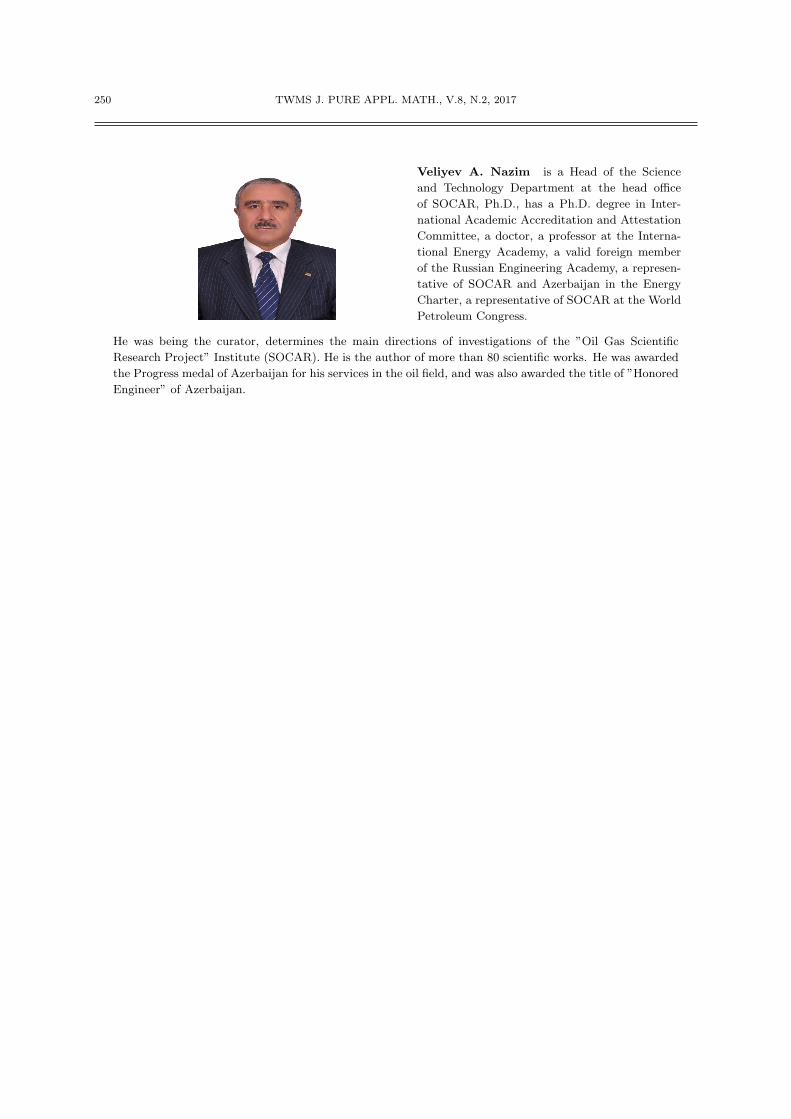
Veliyev A. Nazim is a Head of the Science

and Technology Department at the head office

of SOCAR, Ph.D., has a Ph.D. degree in Inter-

national Academic Accreditation and Attestation

Committee, a doctor, a professor at the Interna-

tional Energy Academy, a valid foreign member

of the Russian Engineering Academy, a represen-

tative of SOCAR and Azerbaijan in the Energy

Charter, a representative of SOCAR at the World

Petroleum Congress.

He was being the curator, determines the main directions of investigations of the ”Oil Gas Scientific

Research Project” Institute (SOCAR). He is the author of more than 80 scientific works. He was awarded

the Progress medal of Azerbaijan for his services in the oil field, and was also awarded the title of ”Honored

Engineer” of Azerbaijan.

the technique of early determination of reservoir drive of...

Documents