the term structure of - newyorkfed.org
TRANSCRIPT
The Term Structure of Expectations
Richard K. Crump | Stefano Eusepi | Emanuel Moench | Bruce Preston
NO. 9 92
NOVEMBER 202 1
The Term Structure of Expectations
Richard K. Crump, Stefano Eusepi, Emanuel Moench, and Bruce Preston
Federal Reserve Bank of New York Staff Reports, no. 992
November 2021
JEL classification: D83, D84, E32, E43, E44, G12
Abstract
Economic theory predicts that intertemporal decisions depend critically on expectations about future
outcomes. Using the universe of professional survey forecasts for the United States, we document the
behavior of the entire term structure of expectations for output growth, inflation, and the policy rate. We
show that a simple unobserved components model of the trend and cycle explains the joint behavior of
both consensus measures of expectations and the observed disagreement among individual forecasters.
Importantly, univariate models of each variable are outperformed by a multivariate model of the joint
dynamics of these three variables, particularly for nominal interest rates. Consistent with the data, the
model predicts a link between revisions in long-run expectations to short-term forecast errors. In
structural models, learning about the long run has important empirical and theoretical implications for
monetary and fiscal policy.
Key words: expectation formation, imperfect information, survey forecasts, shifting endpoint models,
monetary policy, term premiums
_________________
Crump: Federal Reserve Bank of New York (email: [email protected]). Eusepi: University of Texas at Austin (email: [email protected]). Moench: Deutsche Bundesbank, Goethe University, and CEPR (email: [email protected]). Preston: University of Melbourne (email: [email protected]). This paper is a draft chapter for the Handbook of Economic Expectations, Volume 1, edited by R. Bachmann, G. Topa, and W. van der Klaauw. Oliver Kim and Nick Ritter provided excellent research assistance. This paper presents preliminary findings and is being distributed to economists and other interested readers solely to stimulate discussion and elicit comments. The views expressed in this paper are those of the author(s) and do not necessarily reflect the position of the Federal Reserve Bank of New York, the Federal Reserve System, the Deutsche Bundesbank, or the Eurosystem. Any errors or omissions are the responsibility of the author(s). To view the authors’ disclosure statements, visit https://www.newyorkfed.org/research/staff_reports/sr992.html.
Contents
1 Introduction 1
2 Short-Term and Long-Term Forecasts: New Stylized Facts 4
2.1 Motivation: A Simple Model of Long-term Drift . . . . . . . . . . . . . . . . . . . . . . . . . 4
2.1.1 Modeling a Drift in the Long-run Mean . . . . . . . . . . . . . . . . . . . . . . . . . . 5
2.1.2 A More General Setup . . . . . . . . . . . . . . . . . . . . . . . . . . . . . . . . . . . . 6
2.2 Some New Stylized Facts on Individual Forecasts . . . . . . . . . . . . . . . . . . . . . . . . . 7
2.2.1 Properties of Long-Run Forecasts . . . . . . . . . . . . . . . . . . . . . . . . . . . . . . 7
2.2.2 Long-Run Forecast Revisions and Short-Run Forecast Errors . . . . . . . . . . . . . . 10
3 Joint Behavior of Short-Term and Long-Term Forecasts 13
3.1 A Model to Fit the Term Structure of Expectations . . . . . . . . . . . . . . . . . . . . . . . 13
3.1.1 Baseline Multivariate Model . . . . . . . . . . . . . . . . . . . . . . . . . . . . . . . . . 13
3.1.2 Data Overview . . . . . . . . . . . . . . . . . . . . . . . . . . . . . . . . . . . . . . . . 14
3.2 Mapping the Model to Survey Forecasts . . . . . . . . . . . . . . . . . . . . . . . . . . . . . . 17
3.3 Estimation . . . . . . . . . . . . . . . . . . . . . . . . . . . . . . . . . . . . . . . . . . . . . . 18
3.4 Discussion . . . . . . . . . . . . . . . . . . . . . . . . . . . . . . . . . . . . . . . . . . . . . . . 20
3.5 Results . . . . . . . . . . . . . . . . . . . . . . . . . . . . . . . . . . . . . . . . . . . . . . . . . 21
3.5.1 Model Fit . . . . . . . . . . . . . . . . . . . . . . . . . . . . . . . . . . . . . . . . . . . 21
3.5.2 Evolution of the Term Structure of Expectations . . . . . . . . . . . . . . . . . . . . . 25
3.5.3 Perceived Natural Rate of Interest . . . . . . . . . . . . . . . . . . . . . . . . . . . . . 27
4 Expectations and the Term Structure of Interest Rates 31
4.1 Decomposing The Term Structure of Interest Rates . . . . . . . . . . . . . . . . . . . . . . . . 31
4.2 Expectations and Term Premiums . . . . . . . . . . . . . . . . . . . . . . . . . . . . . . . . . 35
5 The Term Structure of Disagreement 43
5.1 Disagreement About the Short Rate, Real Output Growth, and Inflation . . . . . . . . . . . . 43
5.2 What Drives Disagreement About the Short Rate? . . . . . . . . . . . . . . . . . . . . . . . . 45
5.3 Interest Rate Disagreement and the Term Premium . . . . . . . . . . . . . . . . . . . . . . . 48
6 The Term Structure of Expectations in Structural Models 52
6.1 A General Structural Model . . . . . . . . . . . . . . . . . . . . . . . . . . . . . . . . . . . . . 52
6.2 Application 1: Anchored Inflation Expectation . . . . . . . . . . . . . . . . . . . . . . . . . . 54
6.3 Application 2: The Term Structure of Expectations . . . . . . . . . . . . . . . . . . . . . . . . 56
6.4 Implications for Monetary and Fiscal policy . . . . . . . . . . . . . . . . . . . . . . . . . . . . 60
7 Conclusions and Further Directions 61
Appendix A Defining Term Premiums 69
Appendix B Additional Results 70

1 Introduction
Economic theory predicts that intertemporal decisions depend critically on expectations about
future outcomes. Over the past two decades, a concerted research program measures household, firm
and policymaker beliefs using numerous data sources, including surveys, asset prices and controlled
experiments. By dint of this effort, we have invaluable data that can be used to evaluate alternative
theories of expectations formation and their implications for macroeconomics and finance.
Yet the vast majority of this work has focused on expectations about short-term economic de-
velopments. This choice is partly driven by what data are available, as there is substantially less
information on long-run forecasts. But it also reflects the common assumption in macroeconomic
models that economic agents operate in a stationary environment and, consequently, that they can
quickly and efficiently come to understand the long-run behavior of the economy. Any information
frictions that might be relevant to the expectation formation process, are only relevant to short-run
economic dynamics.
These assumptions, however, belie the considerable uncertainty that confronts decision makers
in practice. Indeed, direct survey evidence clearly reveals that expectations about the long-run
values of economic and financial variables vary over time. For example, the Survey of Professional
Forecasters annually queries respondents on their value of the non-accelerating inflation rate of
unemployment, the Federal Reserve Bank of New York’s Survey of Primary Dealers includes ques-
tions on “longer-run” values of economic variables such as output, inflation and the target interest
rate, and the FOMC members themselves report, in the Survey of Economic Projections, the value
that key macroeconomic variables would be expected to converge to under appropriate monetary
policy and in the absence of further shocks to the economy. All of these long-run forecasts display
substantial variation over time.
Movements in long-term expectations are not without consequence. Prominent debates in macroe-
conomics and finance rest on the nature of the long-term behavior of the economy. The seminal
contribution of Lucas (2003) argued that the economic costs of short-term fluctuations pale in
comparison to the implications of long-run growth, underscoring the need to study long-term ex-
pectations and their impact on economic decisions. Among academics and policymakers there is
widespread agreement that the ability of central banks and fiscal authorities to manage business
cycles depends on the maintenance of long-term fiscal sustainability and stable long-run inflation
expectations. And a growing literature in finance understands movements in asset prices by link-
ing them to changes in perceived long-run risk, again highlighting the need to understand market
participants’ shifting views about the long run (e.g., Bansal and Yaron (2004)).
In this chapter we use survey measures of U.S. professional forecasters. One key advantage of
using professional forecasts is the wealth of available data in the U.S. and other countries. Multiple
surveys covering a wide range of forecast horizons spanning “nowcasts” to the very long run are
available. And unlike the growing number of new surveys of households and firms that have become
available to researchers only in recent years, data on professional forecasts have been collected
since at least the mid-1950s. Using these data we document the evolution of the entire term
1

structure of expectations since the 1980s and propose a simple expectations formation mechanism
that rationalizes their behavior. Armed with this framework, we evaluate some implications in a
standard New Keynesian dynamics general equilibrium model.
We show professional forecast data display three important stylized facts. First, long-run expec-
tations about economic variables such as output growth, inflation and short-term nominal interest
rates fluctuate significantly over time, tracking perceived slow-moving changes in the economy such
as the long-run mean of inflation or the natural rate of interest.
Second, the individual components of the term structure of expectations display a clear pattern
of co-movement across different variables and forecast horizons. Changes in long-term expectations
are tied to short-term forecast errors, consistent with an expectations formation mechanism where
agents estimate unobserved trend and cycle components from available data. At the same time,
agents appear to form expectations about macroeconomic variables jointly, so that, for example,
policy rate forecasts are tightly linked to inflation and output growth forecasts.
Third, individual long-term forecasts show a high degree of dispersion for all variables considered
and for all forecasting horizons. This is consistent with economic agents facing fundamental un-
certainty about the long-run behavior of the economy. For example, market participants disagree
more about the long-run determinants of the policy rate, while they display fairly uniform views
about short-term policy expectations.
Throughout the paper we use a model of expectations formation that is consistent with these
observations. While we discuss the literature on the term structure of expectations throughout the
chapter, our primary aim is not to provide an exhaustive summary of existing work. Recent research
covers a wide range of theories that can potentially account for some of the empirical regularities
in survey data. Here we focus on a specific class of information friction, and, therefore, a specific
modeling approach, and discuss its implications for different aspects of the data. On empirical
grounds, we introduce novel data sources together with a number of new empirical results which
shine light on the behavior of expectations across forecast horizons.
This chapter is structured in five broad sections. Section 2 introduces our workhorse model of
the expectations formation mechanism and the information frictions at its foundations. This is
an unobserved components model of the trend and cycle which agents estimate using standard
filtering methods. We then discuss novel survey evidence in support of these assumptions. Using
a cross-section of professional forecasters we document how individual long-term expectations are
revised partly in response to recent forecast errors.
In Section 3 we present a parsimonious monthly vector autoregression model with a time-varying
long-run mean. The model captures the key aspects of our theory and accounts for the joint term
structure of consensus expectations of output growth, inflation and the policy rate. The forecast
data are measured from the universe of professional forecasts for the United States in the post-war
era. We establish that a drifting long-run mean is essential to capture the low-frequency adjustment
in long-run beliefs. Moreover, the multivariate model provides a far superior fit when compared
to a univariate model specification for each variable. This suggests that the dynamic behavior of
2
survey forecasts of different macroeconomic variables need to be modeled jointly. Existing studies
often focus on expectations about an individual variable.
The empirical model delivers tightly estimated forecast paths for these variables at each point
in time over the sample from 1983 through 2019. This novel measure of consensus expectations
enables us to track the evolution of the term structure of expectations since the mid-1980s. For
example, we document the evolution of nominal and real expected interest rates over the monetary
cycle; the adjustment of interest rate expectations in the aftermath of the financial crisis; and the
gradual decline of the perceived natural rate of interest over the past ten years.
Section 4 focuses specifically on the term structure of interest rates, the primary component of
the monetary policy transmission mechanism. We use our measure of expectations to evaluate
the expectations hypothesis, stating that yields on government bonds reflect the average short
rate that investors expect to prevail over the life of the bond. We compare the behavior of the
term structure of consensus expectations with that of the term structure of interest rates derived
from the U.S. Treasury yield curve. Despite the observed volatility of expectations, there remains
substantial unexplained variation at the long-end of the yield curve. We obtain the term premium
as the residual between observed yields and average expected future short rates. The survey-based
measure of the term premium does not co-move in any meaningful way with the term structure
of expectations. This finding begs research on how term premia transmit changes in the stance of
monetary policy.
While having a measure of consensus expectations is an important contribution in its own right
and useful in many economic applications, it neglects the wide dispersion in individual forecasts
documented for professional forecasters, households, firms and policymakers. The heterogeneity in
information can play an important role in explaining the aggregate behavior of the macroeconomy
and asset prices. Section 5 uses data on individual professional forecasters to measure the term
structure of disagreement, or the average disagreement about output growth, inflation and the pol-
icy rate at different forecast horizons. We show that our modeling framework is broadly consistent
with the behavior of both the consensus measure and the cross-section of professional forecasts.
Turning our attention back to the term structure of interest rates, we use our model of expecta-
tions formation to investigate the factors behind the observed dispersion in interest rate forecasts,
especially in the long run. In addition, we show a connection between forecasters’ disagreement
about the path of the policy rate and our measure of the term premium and discuss the implications
for asset pricing in a term structure model that allows explicitly for long-run forecast dispersion.
Most of the analysis conducted in this chapter is based on a reduced-form model of the ex-
pectations formation process. This has the advantage of sidestepping detailed assumptions about
information frictions and, in particular, taking a stand on the rationality of expectations. There are
notable advantages, however, to a more structural approach. Dynamic general equilibrium models
incorporating specific deviations from rationality have greatly helped improving our understanding
of business cycles, asset prices and inflation dynamics. Moreover, structural models are required to
address key questions of monetary and fiscal policy design under different assumptions about how
3
expectations are formed.
Section 6 presents a dynamic structural general equilibrium model where agents are boundedly
rational and have to learn about a possibly changing economic environment. Subjective beliefs
of households and firms are consistent with our reduced-form forecasting model based on survey
evidence. However, the structural model assumes a specific deviation from the full information
rational expectations setup: subjective and objective (model consistent) forecasting models differ.
In particular, subjective beliefs are more persistent than the true data generating process. House-
hold and firm expectations exhibit extrapolation bias, consistent with empirical and laboratory
evidence. Having a structural theory of long-term expectations permits analysis of important prac-
tical policy questions. For example, we argue that our framework provides a coherent definition of
anchored expectations, and clear predictions of the economic conditions under which expectations
will be anchored or unanchored. Finally we discuss the implications of this expectations formation
mechanism for monetary and fiscal policy.
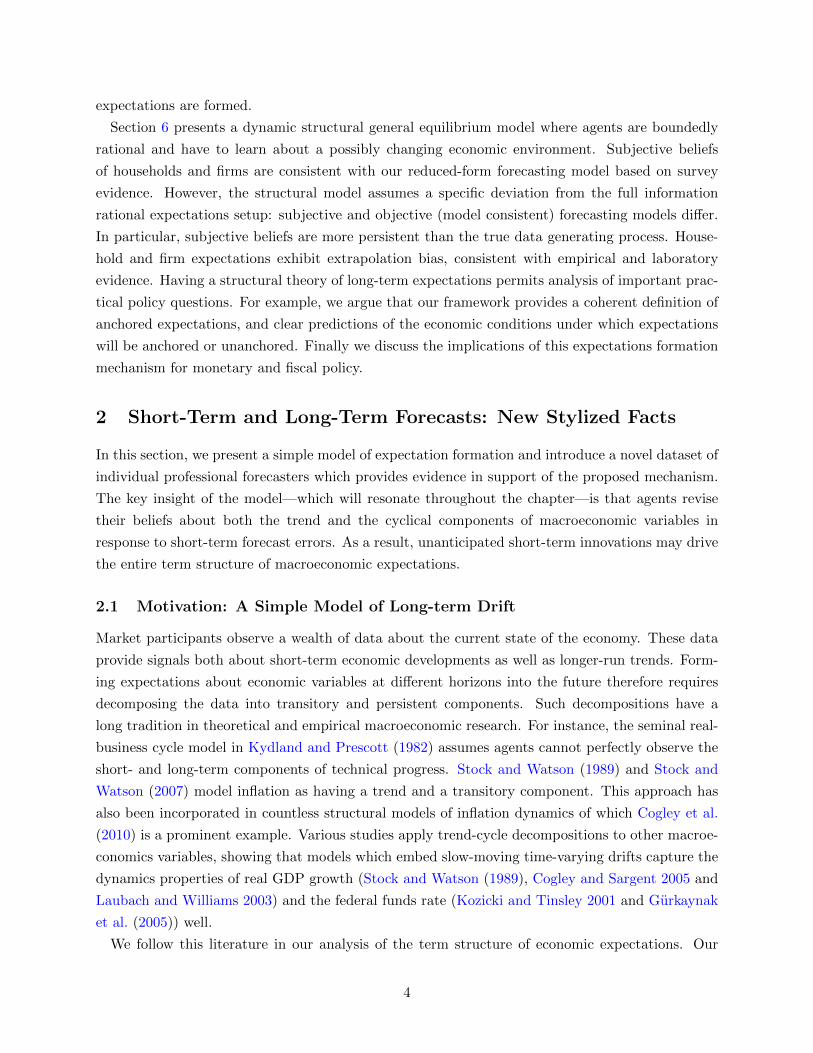
2 Short-Term and Long-Term Forecasts: New Stylized Facts
In this section, we present a simple model of expectation formation and introduce a novel dataset of
individual professional forecasters which provides evidence in support of the proposed mechanism.
The key insight of the model—which will resonate throughout the chapter—is that agents revise
their beliefs about both the trend and the cyclical components of macroeconomic variables in
response to short-term forecast errors. As a result, unanticipated short-term innovations may drive
the entire term structure of macroeconomic expectations.
2.1 Motivation: A Simple Model of Long-term Drift
Market participants observe a wealth of data about the current state of the economy. These data
provide signals both about short-term economic developments as well as longer-run trends. Form-
ing expectations about economic variables at different horizons into the future therefore requires
decomposing the data into transitory and persistent components. Such decompositions have a
long tradition in theoretical and empirical macroeconomic research. For instance, the seminal real-
business cycle model in Kydland and Prescott (1982) assumes agents cannot perfectly observe the
short- and long-term components of technical progress. Stock and Watson (1989) and Stock and
Watson (2007) model inflation as having a trend and a transitory component. This approach has
also been incorporated in countless structural models of inflation dynamics of which Cogley et al.
(2010) is a prominent example. Various studies apply trend-cycle decompositions to other macroe-
conomics variables, showing that models which embed slow-moving time-varying drifts capture the
dynamics properties of real GDP growth (Stock and Watson (1989), Cogley and Sargent 2005 and
Laubach and Williams 2003) and the federal funds rate (Kozicki and Tinsley 2001 and Gurkaynak
et al. (2005)) well.
We follow this literature in our analysis of the term structure of economic expectations. Our
4
approach embeds a key information friction that determines how new information is incorporated
into expectations at different horizons. We argue this model provides an impressive account of
economic expectations which we measure using survey data from professional forecasts.
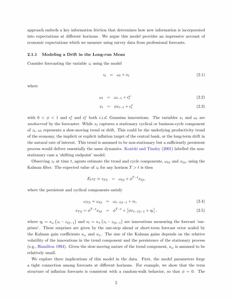
2.1.1 Modeling a Drift in the Long-run Mean
Consider forecasting the variable zt using the model
zt = ωt + xt (2.1)
where
ωt = ωt−1 + εωt (2.2)
xt = φxt−1 + εxt (2.3)
with 0 < φ < 1 and εxt and εωt both i.i.d. Gaussian innovations. The variables xt and ωt are
unobserved by the forecaster. While xt captures a stationary cyclical or business-cycle component
of zt, ωt represents a slow-moving trend or drift. This could be the underlying productivity trend
of the economy, the implicit or explicit inflation target of the central bank, or the long-term drift in
the natural rate of interest. This trend is assumed to be non-stationary but a sufficiently persistent
process would deliver essentially the same dynamics. Kozicki and Tinsley (2001) labelled the non-
stationary case a ‘shifting endpoint’ model.
Observing zt at time t, agents estimate the trend and cycle components, ωt|t and xt|t, using the
Kalman filter. The expected value of zt for any horizon T > t is then
EtzT ≡ zT |t = ωt|t + φT−txt|t,
where the persistent and cyclical components satisfy
ωT |t = ωt|t = ωt−1|t−1 + νt, (2.4)
xT |t = φT−txt|t = φT−t ×[φxt−1|t−1 + ηt
], (2.5)
where ηt = κω(zt − zt|t−1
)and νt = κx
(zt − zt|t−1
)are innovations measuring the forecast ‘sur-
prises’. These surprises are given by the one-step ahead or short-term forecast error scaled by
the Kalman gain coefficients κω and κx. The size of the Kalman gains depends on the relative
volatility of the innovations in the trend component and the persistence of the stationary process
(e.g., Hamilton 1994). Given the slow-moving nature of the trend component, κω is assumed to be
relatively small.
We explore three implications of this model in the data. First, the model parameters forge
a tight connection among forecasts at different horizons. For example, we show that the term
structure of inflation forecasts is consistent with a random-walk behavior, so that φ = 0. The
5
entire term structure of inflation expectations shifts in response to revisions in the estimate ωt|t.
In contrast, interest rate forecasts at short horizons largely reflect a persistent cyclical component,
while long-term forecasts are tied to the drift component.
Second, the model implies a tight connection between long-run forecasts and short-term forecast
errors. To see this, for a forecast horizon T ∗ > t sufficiently large that the cyclical component
becomes unimportant, that is φT∗−t ≈ 0, we have
EtzT ∗ ≈ ωt|t.
Using the law of motion for the estimated trend component in (2.4), the change in longer-term
forecasts is tied to short-term forecast errors or surprises
EtzT ∗ − Et−1zT ∗ ≈ ωt|t − ωt|t−1 = κω(zt − zt|t−1
).
A forecaster that under-predicts zt for few periods should thus revise upwards their long-term
forecast, reflecting a perceived increase in the estimated unobserved drift component.
Third, the model predicts a strong correlation, in this simple example perfect, between the
updates to the trend and cycle components, as they both depend on the same forecast error:
zt − zt|t−1.
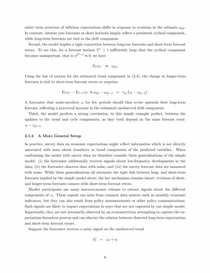
2.1.2 A More General Setup
In practice, survey data on economic expectations might reflect information which is not directly
associated with news about transitory or trend components of the predicted variables. When
confronting the model with survey data we therefore consider three generalizations of the simple
model: (i) the forecaster additionally receives signals about low-frequency developments in the
data; (ii) the forecaster observes data with noise; and (iii) the survey forecast data are measured
with noise. While these generalizations all attenuate the tight link between long- and short-term
forecasts implied by the simple model above, the key mechanism remains intact: revisions of short-
and longer-term forecasts comove with short-term forecast errors.
Market participants use many macroeconomic releases to extract signals about the different
components of zt. These signals can arise from common data sources such as monthly economic
indicators, but they can also result from policy announcements or other policy communications.
Such signals are likely to impact expectations in ways that are not captured by our simple model.
Importantly, they are not necessarily observed by an econometrician attempting to capture the ex-
pectations formation process and can obscure the relation between observed long-term expectations
and short-term forecast errors.
Suppose the forecaster receives a noisy signal on the unobserved trend
sωt = ωt + ot
6

where ot denotes uninformative i.i.d. Gaussian noise. Forecast updating now depends on two
observables, sωt and zt, weakening the link between updates in longer-term forecasts and observed
short-term forecast errors. Revisions to long-dated expectations are
EtzT ∗ − Et−1zT ∗ ≈ κω,z(zt − zt|t−1
)+ κω,s
(sωt − sωt|t−1
).
Furthermore, the presence of such signals weakens the correlation between “innovations” νt and ηt
as they are now represented by different linear combinations of forecast errors and signals.
A common additional informational friction is that the current state zt is not fully observed by
forecasters. Instead, agents may have access to a noisy signal szt = zt + ozt , leading to the updating
equation
EtzT ∗ − Et−1zT ∗ ≈ κω,z(szt − zt|t−1
)= κω,z
(zt − zt|t−1
)+ κω,zo
zt .
Again, the link between forecast errors observed by the econometrician and revisions of longer-
run forecasts is weaker than in the simple model. A different interpretation of the above is that
forecasters use “judgment” when forming forecasts, especially in the short-term. For example, we
can re-write the forecast as
EtzT = EtzT + γT−tτt
where for simplicity τt is described as a first-order autoregressive process, with 0 < γ < 1, capturing
any adjustment to short-term forecasts. In this case
EtzT ∗ − Et−1zT ∗ ≈ κω,z(zt − zt|t−1
)= κω,y
(zt − zt|t−1
)+ κω,zτt
where zt|t−1 is the forecast observed by the econometrician inclusive of judgment. However, the
long-term forecast is computed using the model and does not include the judgment component.
This process also breaks the perfect correlation between observed long-term forecast revisions and
short-term forecast errors.
Finally, survey-based forecasts are informative about the expectation formation process, but are
likely to be measured with error, further complicating the econometrician’s inference problem. This
is discussed in more detail in Section 3.
2.2 Some New Stylized Facts on Individual Forecasts
2.2.1 Properties of Long-Run Forecasts
The model sketched above provides a simple framework to think about the evolution of agents’
forecasts at different horizons. However, because of data limitations there is scant evidence on
individuals’ term structure of expectations, particularly in the context of long-run forecasts. Most
surveys that ask respondents about their beliefs far in the future aggregate the individual survey
7

responses and provide only limited summary statistics.1 Here we exploit a unique data set of indi-
vidual long-run forecasts from the Blue Chip Economic Indicators (BCEI) survey, which provides
the individual responses to the “Long-Range Consensus U.S. Economic Projections” summarized
in the March and October issues. Our data cover the sample period from 1998 to 2016 and all of
the variables queried by the BCEI. We focus on the following set of key macroeconomic indicators:
nominal GDP, real GDP, CPI inflation, the 3-month Treasury Bill rate, and the real 3-month rate
defined as the difference between the nominal rate and CPI inflation. From October 1998 and
March 2006, we can link these individual forecasts to the associated short-run forecasts. However,
outside this data range, we can only link forecasters across variables and horizon, not across survey
dates. Nonetheless, the richness of these data allow us to introduce a number of new stylized facts
about individual long-run forecasts.
To start, Figure 1 shows the consensus (i.e., cross-sectional mean) forecast for two selected
horizons based on the BCEI survey, namely, three-years ahead and the average of seven-to-eleven
years ahead. The sample period covers the 40 years ending in 2019. In these charts we observe
two key features of these forecasts. First, the forecasts for the two horizons broadly comove,
with the three-year ahead forecast generally displaying more high-frequency variability. Second,
the longest-horizon forecast, predicting these key economic variables seven-to-eleven years in the
future, clearly varies over time. For example, the long-horizon consensus forecast for real output
growth varies between more than 3% and a bit below 2.5%, and then falls to below 2% after the
Global Financial Crisis (top left chart). More dramatically, the long-run forecast for CPI inflation
and the 3-month T-bill exhibit strong secular declines throughout the sample (top right and lower
left chart). Despite sharing that broad-based secular decline, their difference, the real 3-month T-
bill, shows variation throughout and ends the sample at about 0%. In sum, Figure 1 provides clear
evidence that long-horizon forecasts show meaningful variation over time, in line with forecasters
updating their estimates of the trend components of the observed data.
1For example, both the Blue Chip Financial Forecasts and the BCEI present the cross-sectional average alongwith the average of the top-10 forecasters and bottom-10 forecasters at each forecast horizon. As another example,the Survey of Primary Dealers (SPD) provides the cross-sectional median along with the 25th and 75th percentiles.
8
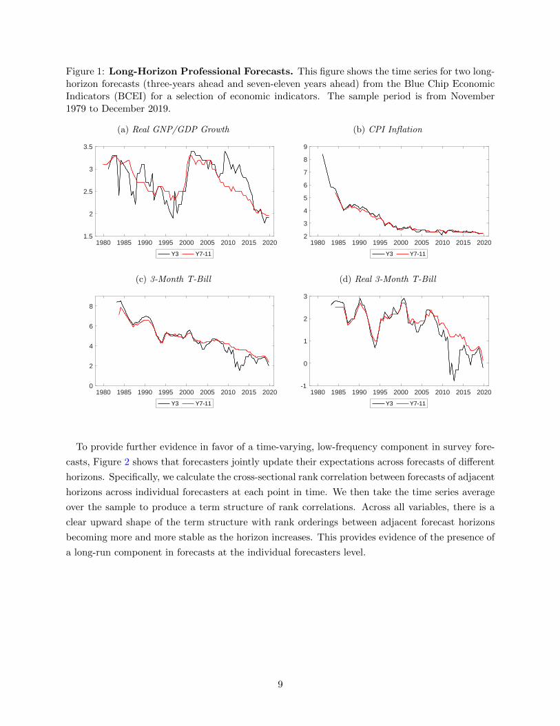
Figure 1: Long-Horizon Professional Forecasts. This figure shows the time series for two long-horizon forecasts (three-years ahead and seven-eleven years ahead) from the Blue Chip EconomicIndicators (BCEI) for a selection of economic indicators. The sample period is from November1979 to December 2019.
(a) Real GNP/GDP Growth
1980 1985 1990 1995 2000 2005 2010 2015 20201.5
2
2.5
3
3.5
Y3 Y7-11
(b) CPI Inflation
1980 1985 1990 1995 2000 2005 2010 2015 20202
3
4
5
6
7
8
9
Y3 Y7-11
(c) 3-Month T-Bill
1980 1985 1990 1995 2000 2005 2010 2015 20200
2
4
6
8
Y3 Y7-11
(d) Real 3-Month T-Bill
1980 1985 1990 1995 2000 2005 2010 2015 2020-1
0
1
2
3
Y3 Y7-11
To provide further evidence in favor of a time-varying, low-frequency component in survey fore-
casts, Figure 2 shows that forecasters jointly update their expectations across forecasts of different
horizons. Specifically, we calculate the cross-sectional rank correlation between forecasts of adjacent
horizons across individual forecasters at each point in time. We then take the time series average
over the sample to produce a term structure of rank correlations. Across all variables, there is a
clear upward shape of the term structure with rank orderings between adjacent forecast horizons
becoming more and more stable as the horizon increases. This provides evidence of the presence of
a long-run component in forecasts at the individual forecasters level.
9
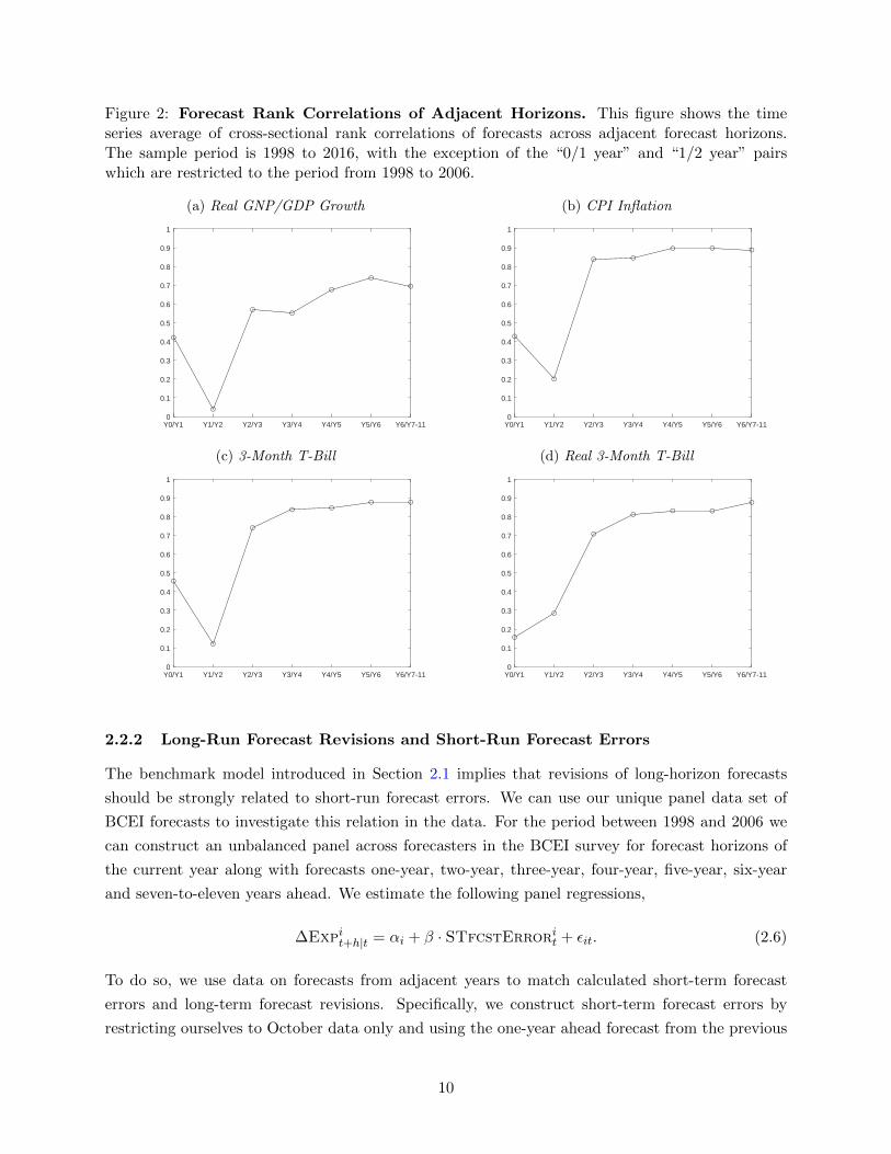
Figure 2: Forecast Rank Correlations of Adjacent Horizons. This figure shows the timeseries average of cross-sectional rank correlations of forecasts across adjacent forecast horizons.The sample period is 1998 to 2016, with the exception of the “0/1 year” and “1/2 year” pairswhich are restricted to the period from 1998 to 2006.
(a) Real GNP/GDP Growth
Y0/Y1 Y1/Y2 Y2/Y3 Y3/Y4 Y4/Y5 Y5/Y6 Y6/Y7-110
0.1
0.2
0.3
0.4
0.5
0.6
0.7
0.8
0.9
1
(b) CPI Inflation
Y0/Y1 Y1/Y2 Y2/Y3 Y3/Y4 Y4/Y5 Y5/Y6 Y6/Y7-110
0.1
0.2
0.3
0.4
0.5
0.6
0.7
0.8
0.9
1
(c) 3-Month T-Bill
Y0/Y1 Y1/Y2 Y2/Y3 Y3/Y4 Y4/Y5 Y5/Y6 Y6/Y7-110
0.1
0.2
0.3
0.4
0.5
0.6
0.7
0.8
0.9
1
(d) Real 3-Month T-Bill
Y0/Y1 Y1/Y2 Y2/Y3 Y3/Y4 Y4/Y5 Y5/Y6 Y6/Y7-110
0.1
0.2
0.3
0.4
0.5
0.6
0.7
0.8
0.9
1
2.2.2 Long-Run Forecast Revisions and Short-Run Forecast Errors
The benchmark model introduced in Section 2.1 implies that revisions of long-horizon forecasts
should be strongly related to short-run forecast errors. We can use our unique panel data set of
BCEI forecasts to investigate this relation in the data. For the period between 1998 and 2006 we
can construct an unbalanced panel across forecasters in the BCEI survey for forecast horizons of
the current year along with forecasts one-year, two-year, three-year, four-year, five-year, six-year
and seven-to-eleven years ahead. We estimate the following panel regressions,
∆Expit+h|t = αi + β · STfcstErrorit + εit. (2.6)
To do so, we use data on forecasts from adjacent years to match calculated short-term forecast
errors and long-term forecast revisions. Specifically, we construct short-term forecast errors by
restricting ourselves to October data only and using the one-year ahead forecast from the previous
10

October to the current “nowcast” for the contemporaneous year.2 To construct the change in
long-horizon forecasts, we simply take the difference between the current forecast and that of the
previous October. Thus, we can use the year pairs, {1998/1999}, {1999/2000}, · · · , {2004/2005} for
a total of T = 7 pairs. There are 48 forecasting firms in the data, but not all firms forecast for each
year and may not provide forecasts for all variables. In sum, there are a total of 164 observations
at the year-firm level.
Figure 3: Forecast Errors and Forecast Revisions. This figure shows scatterplots of short-term forecast errors against revisions in long-run forecasts based on the BCEI data. The sampleperiod is October 1998 to October 2005.
(a) Real GNP/GDP Growth (b) CPI Inflation
(c) 3-Month T-Bill (d) Real 3-Month T-Bill
Figure 3 displays scatterplots of short-run forecast errors against forecast revisions of long-horizon
2Strictly speaking, not all data have been realized by October, and so these are not exact forecast errors. However,the influence of these observations is small (see Crump et al. 2014). As a robustness check, we added time fixed effectsto our regression specification and find they do not change the qualitative results.
11
forecasts using these individual BCEI panel data for the same four variables as in Figures 1 and 2.
We superimpose the fitted OLS regression line in each of the four scatterplots. In all cases except
for CPI inflation, there is a clear positive correlation between forecast errors and forecast revisions.
Moreover, none of the scatters appear to have notable outliers that might unduly influence estimated
relationships between the two variables.
To provide further evidence of the link between individual forecast revisions at long horizons and
short-term forecast errors, we estimate 16 regression specifications, one for each of the 15 variables
available in our data set, along with the implied forecast for the real 3-month T-bill which we
construct as the difference between the nominal 3-month T-bill and quarterly CPI inflation fore-
casts. Table 1 presents the regression results for a selected set of prominent economic indicators
(see Table A.1 in the Appendix for all results). We report the estimated coefficient, β and the
associated p-value in parentheses below. For most of the 16 considered variables, there is a signifi-
cant correlation between individual forecast errors and long-term forecast revisions. For example,
in the case of real output growth we observe a strongly significant coefficient β suggesting that a
rise in the short-run forecast error of 1 percentage point is associated with about a 1/8 percentage
point rise in the long-run forecast for real GDP growth. More generally, we observe that all esti-
mated coefficients are positive and almost all are statistically significant at standard significance
levels. The estimated coefficients are similar regardless of whether we account for unobserved het-
erogeneity using the fixed-effects estimator or not. These conclusions are essentially unchanged
when evaluating the larger group of indicators available in Table A.1. A notable exception is the
specification for CPI forecasts which possesses positive estimated coefficients, but sufficiently large
standard errors that the p-values are all far from zero. A plausible explanation for this result is
that longer-horizon inflation forecasts have been relatively well anchored and thus insensitive to
incoming economic information since the late 1990s which imply a weaker observed correlation be-
tween observed long-term forecast revisions and short-term forecast errors. Carvalho et al. (2021)
propose a learning model which gives rise to such an insensitivity while at the same time implying
a tight link between long-term forecast revisions and short-term forecast errors from the late 1970s
until the 1990s. We discuss this further in section 6.
Relation to existing literature: A few papers have explored the link between forecast revisions
and forecast errors using pass-through regressions of either macroeconomic news or movements in
short-term expectations to long-term expectations, see for example Gurkaynak et al. (2010) and
Beechey et al. (2011). In addition, Bems et al. (2021) provide time-series evidence of this link for
a large set of countries. To our knowledge, we are the first to use granular panel data to explicitly
demonstrate the link between short-run forecast errors and changes in long-run forecasts at the
individual forecaster level.
12
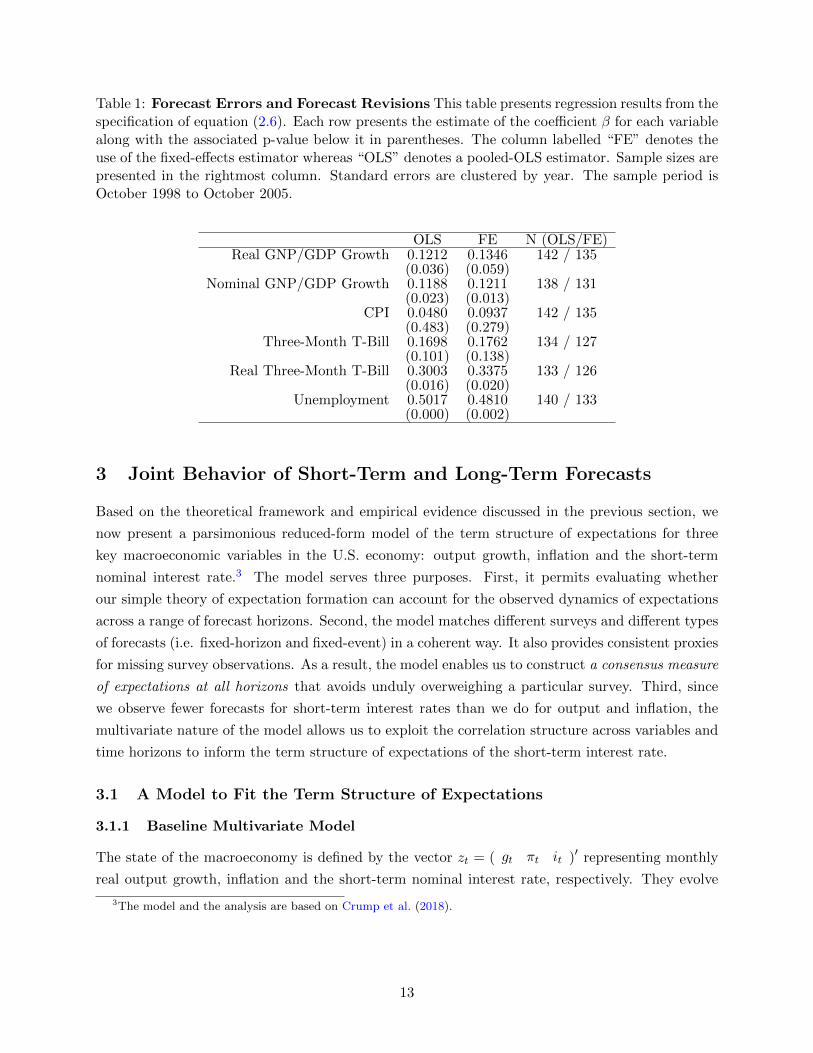
Table 1: Forecast Errors and Forecast Revisions This table presents regression results from thespecification of equation (2.6). Each row presents the estimate of the coefficient β for each variablealong with the associated p-value below it in parentheses. The column labelled “FE” denotes theuse of the fixed-effects estimator whereas “OLS” denotes a pooled-OLS estimator. Sample sizes arepresented in the rightmost column. Standard errors are clustered by year. The sample period isOctober 1998 to October 2005.
OLS FE N (OLS/FE)Real GNP/GDP Growth 0.1212 0.1346 142 / 135
(0.036) (0.059)Nominal GNP/GDP Growth 0.1188 0.1211 138 / 131
(0.023) (0.013)CPI 0.0480 0.0937 142 / 135
(0.483) (0.279)Three-Month T-Bill 0.1698 0.1762 134 / 127
(0.101) (0.138)Real Three-Month T-Bill 0.3003 0.3375 133 / 126
(0.016) (0.020)Unemployment 0.5017 0.4810 140 / 133
(0.000) (0.002)
3 Joint Behavior of Short-Term and Long-Term Forecasts
Based on the theoretical framework and empirical evidence discussed in the previous section, we
now present a parsimonious reduced-form model of the term structure of expectations for three
key macroeconomic variables in the U.S. economy: output growth, inflation and the short-term
nominal interest rate.3 The model serves three purposes. First, it permits evaluating whether
our simple theory of expectation formation can account for the observed dynamics of expectations
across a range of forecast horizons. Second, the model matches different surveys and different types
of forecasts (i.e. fixed-horizon and fixed-event) in a coherent way. It also provides consistent proxies
for missing survey observations. As a result, the model enables us to construct a consensus measure
of expectations at all horizons that avoids unduly overweighing a particular survey. Third, since
we observe fewer forecasts for short-term interest rates than we do for output and inflation, the
multivariate nature of the model allows us to exploit the correlation structure across variables and
time horizons to inform the term structure of expectations of the short-term interest rate.
3.1 A Model to Fit the Term Structure of Expectations
3.1.1 Baseline Multivariate Model
The state of the macroeconomy is defined by the vector zt = ( gt πt it )′ representing monthly
real output growth, inflation and the short-term nominal interest rate, respectively. They evolve
3The model and the analysis are based on Crump et al. (2018).
13
as
xt = Φxt−1 + νt (3.1)
ωt = ωt−1 + ηt (3.2)
zt = ωt + xt (3.3)
where the variables xt ≡ xt|t and ωt ≡ ωt|t are 3× 1 vectors capturing agents’ estimates about the
underlying unobserved states. To keep the model simple, the innovations εt = ( νt ηt )′ are as-
sumed to be i.i.d. across time and are normally distributed with variance covariance Σε. Consistent
with the model presented in Section 2.1, innovations in the drift are potentially correlated with
innovations in the cyclical components of the model. The matrix Φ measures the autocorrelation
properties of the stationary component xt and consequently has eigenvalues in the unit circle. The
model is defined at the monthly frequency which is the highest frequency observed across the range
of surveys of professional forecasts to which we fit the model.
3.1.2 Data Overview
We seek to model the joint term structure of expectations for real output growth, inflation, and
the short-term interest rate. To do this we use the universe of professional forecasts for the United
States in the post-war era, obtained from nine different survey sources: (1) Blue Chip Financial
Forecasts (BCFF); (2) Blue Chip Economic Indicators (BCEI); (3) Consensus Economics (CE); (4)
Decision Makers’ Poll (DMP); (5) Economic Forecasts: A Worldwide Survey (EF); (6) Goldsmith-
Nagan (GN); (7) Livingston Survey (Liv.); (8) Survey of Primary Dealers (SPD); (9) Survey of
Professional Forecasters (SPF). We focus on three sets of forecasts. For output growth we use
forecasts of real GNP growth prior to 1992 and forecasts of real GDP growth thereafter. For
inflation we use forecasts of growth in the consumer price index (CPI). We choose the CPI over
alternative inflation measures such as the GDP deflator because CPI forecasts are available more
frequently and for a longer history than alternative inflation measures. Finally, we use the 3-month
Treasury bill (secondary market) rate as our measure of a short-term interest rate as it is by far
the most frequently surveyed short-term interest rate available.4
Combined, these surveys provide a rich portrait of professional forecasters’ macroeconomic ex-
pectations. Our results are based on 627 variable-horizon pairs spanning the period 1955 to 2019.
While we provide more details about each individual survey in the Appendix, the survey data differ
in frequency, forecast timing, target series, sample availability and forecast horizons. To ease nota-
tion we use the following conventions. Q1 represents a one-quarter ahead forecast, Q2 represents
a two-quarter ahead forecast and so on. Y1 represents a one-year ahead forecast, e.g., a forecast
for the year 2014 made at any time in 2013. Y2 represents a two-year ahead forecast and so on.
Y0-5 represents a forecast for the average value over the years ranging from the current year to five
4For example, forecasts of the Federal Funds rate, the target rate of U.S. monetary policy are only available intwo of the eight surveys we consider (BCFF and SPD).
14
years ahead, e.g., a forecast for the average annual growth rate of GDP from 2014 through 2019
made at any time in 2014. Y1-6, Y2-7 and so on are defined similarly. Y6-10 represents a forecast
for the average value over the years ranging from six years ahead to 10 years ahead, e.g., a forecast
for the average annual growth rate of GDP from 2020 through 2024, made at any time in 2014.
Within each of these sub-categories the exact form of the target variable may vary. For example,
a forecast for the year 2014 may be queried based on annual average growth or Q4/Q4 growth.
As we make clear below, throughout the paper we ensure consistency between model-implied and
observed forecasts with respect to variable definition and forecast horizon.
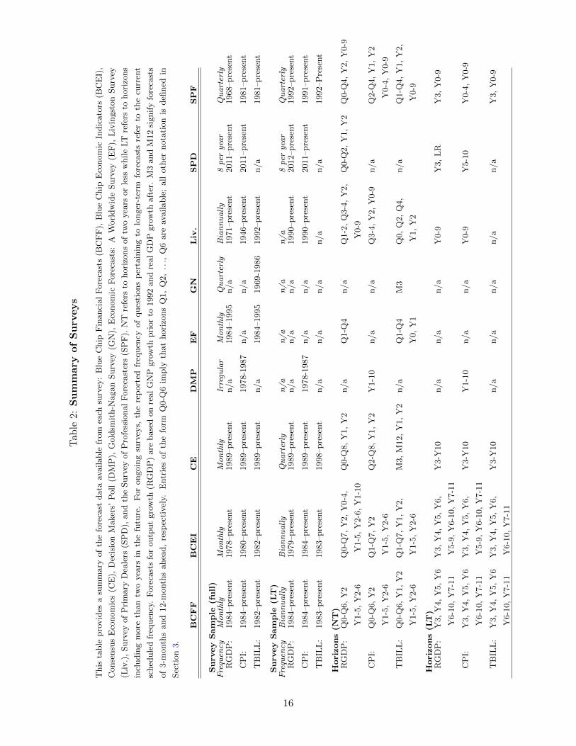
Table 2 summarizes the survey data we use in the paper. Near-term survey forecasts (target
period is up to two years ahead) are available for the longest sample with CPI forecasts from the
Livingston Survey beginning in the mid-1940s. Medium- and long-term forecasts (target period
includes three-years ahead and longer) are available for real output growth and inflation starting
in the late 1970s. However, a more comprehensive set of long-term forecasts (a target period of
five or more years ahead) for all three variables is available only starting in the mid-1980s. At all
horizons there are relatively fewer forecasts for the 3-month Treasury bill than for output growth
and inflation.
In the discussion of our results we focus on the period 1982–2019, covering the Great Moderation,
the Great Recession following the Global Financial Crisis up to the pre-COVID period. This period
includes the majority of the available survey forecasts with over 75% of the total number of series
used available in this 35 year time span.
15
Tab
le2:
Su
mm
ary
of
Su
rveys
This
table
pro
vid
esa
sum
mary
of
the
fore
cast
data
available
from
each
surv
ey:
Blu
eC
hip
Fin
anci
al
Fore
cast
s(B
CF
F),
Blu
eC
hip
Eco
nom
icIn
dic
ato
rs(B
CE
I),
Conse
nsu
sE
conom
ics
(CE
),D
ecis
ion
Maker
s’P
oll
(DM
P),
Gold
smit
h-N
agan
Surv
ey(G
N),
Eco
nom
icF
ore
cast
s:A
Worl
dw
ide
Surv
ey(E
F),
Liv
ingst
on
Surv
ey
(Liv
.),
Surv
eyof
Pri
mary
Dea
lers
(SP
D),
and
the
Surv
eyof
Pro
fess
ional
Fore
cast
ers
(SP
F).
NT
refe
rsto
hori
zons
of
two
yea
rsor
less
while
LT
refe
rsto
hori
zons
incl
udin
gm
ore
than
two
yea
rsin
the
futu
re.
For
ongoin
gsu
rvey
s,th
ere
port
edfr
equen
cyof
ques
tions
per
tain
ing
tolo
nger
-ter
mfo
reca
sts
refe
rto
the
curr
ent
sched
ule
dfr
equen
cy.
Fore
cast
sfo
routp
ut
gro
wth
(RG
DP
)are
base
don
real
GN
Pgro
wth
pri
or
to1992
and
real
GD
Pgro
wth
aft
er.
M3
and
M12
signif
yfo
reca
sts
of
3-m
onth
sand
12-m
onth
sahea
d,
resp
ecti
vel
y.E
ntr
ies
of
the
form
Q0-Q
6im
ply
that
hori
zons
Q1,
Q2,...,
Q6
are
available
;all
oth
ernota
tion
isdefi
ned
in
Sec
tion
3.
BC
FF
BC
EI
CE
DM
PE
FG
NL
iv.
SP
DSP
F
Surv
ey
Sam
ple
(full)
Frequ
ency
Monthly
Monthly
Monthly
Irregu
lar
Monthly
Quarterly
Biannually
8peryear
Quarterly
RG
DP
:1984–pre
sent
1978–pre
sent
1989–pre
sent
n/a
1984–1995
n/a
1971–pre
sent
2011–pre
sent
1968–pre
sent
CP
I:1984–pre
sent
1980–pre
sent
1989–pre
sent
1978-1
987
n/a
n/a
1946–pre
sent
2011–pre
sent
1981–pre
sent
TB
ILL
:1982–pre
sent
1982–pre
sent
1989–pre
sent
n/a
1984–1995
1969-1
986
1992–pre
sent
n/a
1981–pre
sent
Surv
ey
Sam
ple
(LT
)Frequ
ency
Biannually
Biannually
Quarterly
n/a
n/a
n/a
n/a
8peryear
Quarterly
RG
DP
:1984–pre
sent
1979–pre
sent
1989–pre
sent
n/a
n/a
n/a
1990–pre
sent
2012–pre
sent
1992–pre
sent
CP
I:1984–pre
sent
1984–pre
sent
1989–pre
sent
1978-1
987
n/a
n/a
1990–pre
sent
2011–pre
sent
1991–pre
sent
TB
ILL
:1983–pre
sent
1983–pre
sent
1998–pre
sent
n/a
n/a
n/a
n/a
n/a
1992–P
rese
nt
Hori
zons
(NT
)R
GD
P:
Q0-Q
6,
Y2
Q0-Q
7,
Y2,
Y0-4
,Q
0-Q
8,
Y1,
Y2
n/a
Q1-Q
4n/a
Q1-2
,Q
3-4
,Y
2,
Q0-Q
2,
Y1,
Y2
Q0-Q
4,
Y2,
Y0-9
Y1-5
,Y
2-6
Y1-5
,Y
2-6
,Y
1-1
0Y
0-9
CP
I:Q
0-Q
6,
Y2
Q1-Q
7,
Y2
Q2-Q
8,
Y1,
Y2
Y1-1
0n/a
n/a
Q3-4
,Y
2,
Y0-9
n/a
Q2-Q
4,
Y1,
Y2
Y1-5
,Y
2-6
Y1-5
,Y
2-6
Y0-4
,Y
0-9
TB
ILL
:Q
0-Q
6,
Y1,
Y2
Q1-Q
7,
Y1,
Y2,
M3,
M12,
Y1,
Y2
n/a
Q1-Q
4M
3Q
0,
Q2,
Q4,
n/a
Q1-Q
4,
Y1,
Y2,
Y1-5
,Y
2-6
Y1-5
,Y
2-6
Y0,
Y1
Y1,
Y2
Y0-9
Hori
zons
(LT
)R
GD
P:
Y3,
Y4,
Y5,
Y6
Y3,
Y4,
Y5,
Y6,
Y3-Y
10
n/a
n/a
n/a
Y0-9
Y3,
LR
Y3,
Y0-9
Y6-1
0,
Y7-1
1Y
5-9
,Y
6-1
0,
Y7-1
1
CP
I:Y
3,
Y4,
Y5,
Y6
Y3,
Y4,
Y5,
Y6,
Y3-Y
10
Y1-1
0n/a
n/a
Y0-9
Y5-1
0Y
0-4
,Y
0-9
Y6-1
0,
Y7-1
1Y
5-9
,Y
6-1
0,
Y7-1
1
TB
ILL
:Y
3,
Y4,
Y5,
Y6
Y3,
Y4,
Y5,
Y6,
Y3-Y
10
n/a
n/a
n/a
n/a
n/a
Y3,
Y0-9
Y6-1
0,
Y7-1
1Y
6-1
0,
Y7-1
1
16

3.2 Mapping the Model to Survey Forecasts
The model defined by equations (3.1)-(3.3) has the state-space representation
Zt = F (Φ)Zt−1 + V εt
where Zt = ( zt ... zt−4 xt ωt )′. The presence of four lags in zt, facilitates mapping data
definitions to model concepts, as discussed further below. The heterogeneity of available forecasts
makes this a non-trivial task. Start with a simple example. Suppose each month we only observe
survey forecasts at monthly horizons. For example, we might measure a forecast for the n-month-
ahead inflation rate at time t. Using the model, the n-step-ahead forecast of all model variables is
given by
Etzt+n = ωt + Φnxt,
where the model forecast of inflation would be the second element of the vector zt. The larger state
vector satisfies
EtZt+n = F (Φ)n Zt
and provides the observation equation. The mapping between data and model is then straightfor-
ward.
In practice, however, survey participants are rarely asked to provide monthly forecasts. Rather
they are queried about different types of forecasts, which involve quarterly averages, year-over-year
growth rates and so on. When estimating our model we take care to match as closely as possible
the observed forecasts with the correct model representation. The following examples help clarify
how we do this. Consider the short-term interest rate. Forecasts for the three-month Treasury
bill rate are either a simple average over a period or end of period. For the latter we assign these
forecasts to the last month in the period. For real output growth and inflation, survey forecasts
come in three possible forms: quarter-over-quarter annualized growth, annual average growth and
Q4/Q4 growth. Let G2019Q1 and G2019Q2 be the level of real GDP in billions of chained dollars in
the first and second quarter of 2019, respectively. Then, the quarterly average annualized growth
rate is defined as 100 · ((G2019Q2/G2019Q1)4 − 1). Our model variables define a month-over-month
(annualized) real GDP growth rate series. To map the monthly series into this specific measured
quarterly growth rate we follow Crump et al. (2014) and use
100 · ((G2019Q2/G2019Q1)4 − 1) ≈ 1
9(g2019m2 + 2 · g2019m3 + 3 · g2019m4 + 2 · g2019m5 + g2019m6) ,
where, for example, g2019m2 represents the model-based month-over-month annualized real output
growth in February 2019. This notation makes clear why lagged values of zt appear in the state
vector Zt. Annual average growth rates follow a similar pattern. For example, let G2018 and G2019
17
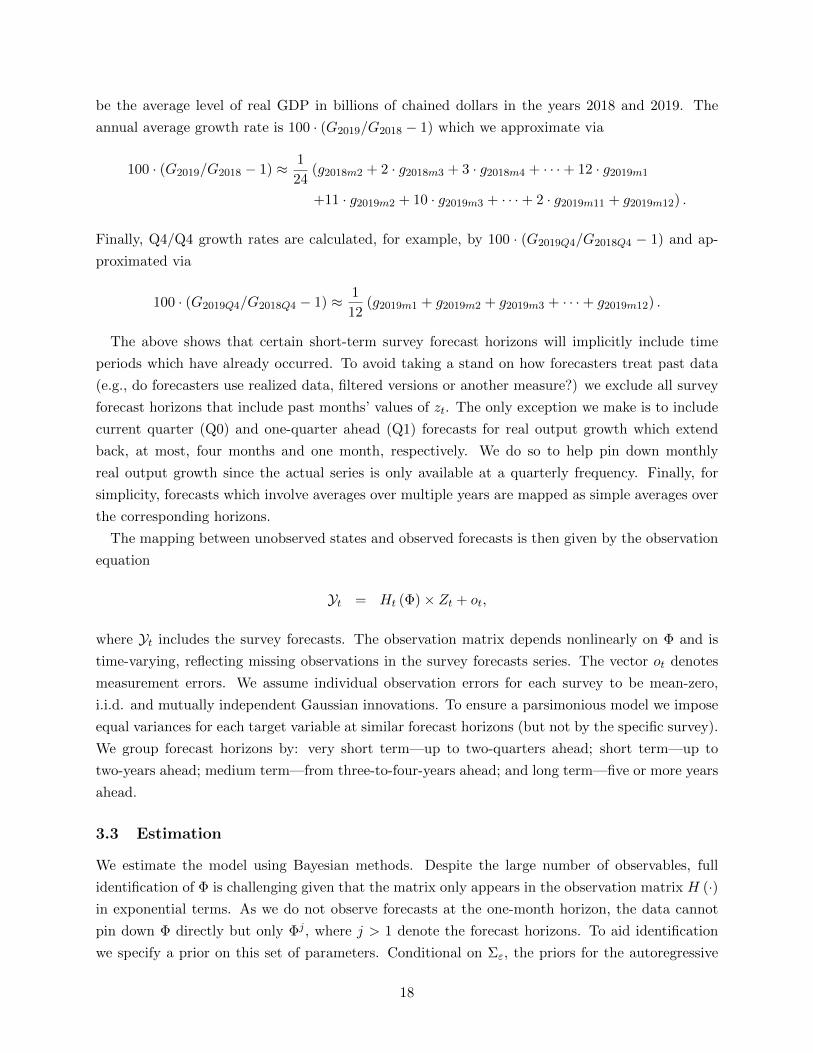
be the average level of real GDP in billions of chained dollars in the years 2018 and 2019. The
annual average growth rate is 100 · (G2019/G2018 − 1) which we approximate via
100 · (G2019/G2018 − 1) ≈ 1
24(g2018m2 + 2 · g2018m3 + 3 · g2018m4 + · · ·+ 12 · g2019m1
+11 · g2019m2 + 10 · g2019m3 + · · ·+ 2 · g2019m11 + g2019m12) .
Finally, Q4/Q4 growth rates are calculated, for example, by 100 · (G2019Q4/G2018Q4 − 1) and ap-
proximated via
100 · (G2019Q4/G2018Q4 − 1) ≈ 1
12(g2019m1 + g2019m2 + g2019m3 + · · ·+ g2019m12) .
The above shows that certain short-term survey forecast horizons will implicitly include time
periods which have already occurred. To avoid taking a stand on how forecasters treat past data
(e.g., do forecasters use realized data, filtered versions or another measure?) we exclude all survey
forecast horizons that include past months’ values of zt. The only exception we make is to include
current quarter (Q0) and one-quarter ahead (Q1) forecasts for real output growth which extend
back, at most, four months and one month, respectively. We do so to help pin down monthly
real output growth since the actual series is only available at a quarterly frequency. Finally, for
simplicity, forecasts which involve averages over multiple years are mapped as simple averages over
the corresponding horizons.
The mapping between unobserved states and observed forecasts is then given by the observation
equation
Yt = Ht (Φ)× Zt + ot,
where Yt includes the survey forecasts. The observation matrix depends nonlinearly on Φ and is
time-varying, reflecting missing observations in the survey forecasts series. The vector ot denotes
measurement errors. We assume individual observation errors for each survey to be mean-zero,
i.i.d. and mutually independent Gaussian innovations. To ensure a parsimonious model we impose
equal variances for each target variable at similar forecast horizons (but not by the specific survey).
We group forecast horizons by: very short term—up to two-quarters ahead; short term—up to
two-years ahead; medium term—from three-to-four-years ahead; and long term—five or more years
ahead.
3.3 Estimation
We estimate the model using Bayesian methods. Despite the large number of observables, full
identification of Φ is challenging given that the matrix only appears in the observation matrix H (·)in exponential terms. As we do not observe forecasts at the one-month horizon, the data cannot
pin down Φ directly but only Φj , where j > 1 denote the forecast horizons. To aid identification
we specify a prior on this set of parameters. Conditional on Σε, the priors for the autoregressive
18
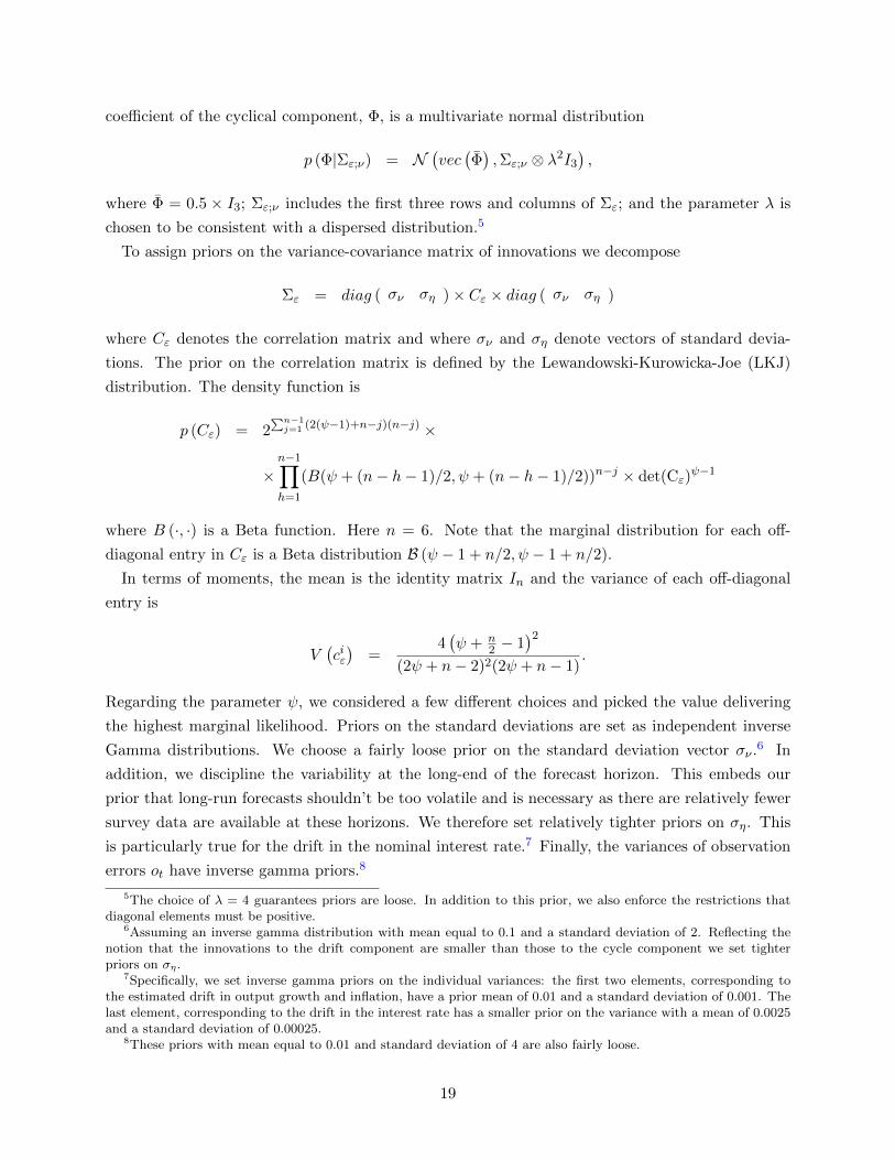
coefficient of the cyclical component, Φ, is a multivariate normal distribution
p (Φ|Σε;ν) = N(vec
(Φ),Σε;ν ⊗ λ2I3
),
where Φ = 0.5 × I3; Σε;ν includes the first three rows and columns of Σε; and the parameter λ is
chosen to be consistent with a dispersed distribution.5
To assign priors on the variance-covariance matrix of innovations we decompose
Σε = diag ( σν ση )× Cε × diag ( σν ση )
where Cε denotes the correlation matrix and where σν and ση denote vectors of standard devia-
tions. The prior on the correlation matrix is defined by the Lewandowski-Kurowicka-Joe (LKJ)
distribution. The density function is
p (Cε) = 2∑n−1j=1 (2(ψ−1)+n−j)(n−j) ×
×n−1∏h=1
(B(ψ + (n− h− 1)/2, ψ + (n− h− 1)/2))n−j × det(Cε)ψ−1
where B (·, ·) is a Beta function. Here n = 6. Note that the marginal distribution for each off-
diagonal entry in Cε is a Beta distribution B (ψ − 1 + n/2, ψ − 1 + n/2).
In terms of moments, the mean is the identity matrix In and the variance of each off-diagonal
entry is
V(ciε)
=4(ψ + n
2 − 1)2
(2ψ + n− 2)2(2ψ + n− 1).
Regarding the parameter ψ, we considered a few different choices and picked the value delivering
the highest marginal likelihood. Priors on the standard deviations are set as independent inverse
Gamma distributions. We choose a fairly loose prior on the standard deviation vector σν .6 In
addition, we discipline the variability at the long-end of the forecast horizon. This embeds our
prior that long-run forecasts shouldn’t be too volatile and is necessary as there are relatively fewer
survey data are available at these horizons. We therefore set relatively tighter priors on ση. This
is particularly true for the drift in the nominal interest rate.7 Finally, the variances of observation
errors ot have inverse gamma priors.8
5The choice of λ = 4 guarantees priors are loose. In addition to this prior, we also enforce the restrictions thatdiagonal elements must be positive.
6Assuming an inverse gamma distribution with mean equal to 0.1 and a standard deviation of 2. Reflecting thenotion that the innovations to the drift component are smaller than those to the cycle component we set tighterpriors on ση.
7Specifically, we set inverse gamma priors on the individual variances: the first two elements, corresponding tothe estimated drift in output growth and inflation, have a prior mean of 0.01 and a standard deviation of 0.001. Thelast element, corresponding to the drift in the interest rate has a smaller prior on the variance with a mean of 0.0025and a standard deviation of 0.00025.
8These priors with mean equal to 0.01 and standard deviation of 4 are also fairly loose.
19
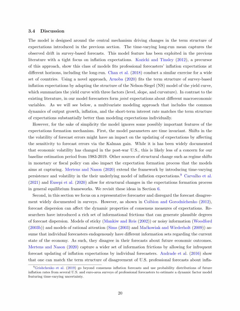
3.4 Discussion
The model is designed around the central mechanism driving changes in the term structure of
expectations introduced in the previous section. The time-varying long-run mean captures the
observed drift in survey-based forecasts. This model feature has been exploited in the previous
literature with a tight focus on inflation expectations. Kozicki and Tinsley (2012), a precursor
of this approach, show this class of models fits professional forecasters’ inflation expectations at
different horizons, including the long-run. Chan et al. (2018) conduct a similar exercise for a wide
set of countries. Using a novel approach, Aruoba (2020) fits the term structure of survey-based
inflation expectations by adapting the structure of the Nelson-Siegel (NS) model of the yield curve,
which summarizes the yield curve with three factors (level, slope, and curvature). In contrast to the
existing literature, in our model forecasters form joint expectations about different macroeconomic
variables. As we will see below, a multivariate modeling approach that includes the common
dynamics of output growth, inflation, and the short-term interest rate matches the term structure
of expectations substantially better than modeling expectations individually.
However, for the sake of simplicity the model ignores some possibly important features of the
expectations formation mechanism. First, the model parameters are time invariant. Shifts in the
the volatility of forecast errors might have an impact on the updating of expectations by affecting
the sensitivity to forecast errors via the Kalman gain. While it is has been widely documented
that economic volatility has changed in the post-war U.S., this is likely less of a concern for our
baseline estimation period from 1983-2019. Other sources of structural change such as regime shifts
in monetary or fiscal policy can also impact the expectation formation process that the models
aims at capturing. Mertens and Nason (2020) extend the framework by introducing time-varying
persistence and volatility in the their underlying model of inflation expectations.9 Carvalho et al.
(2021) and Eusepi et al. (2020) allow for structural changes in the expectations formation process
in general equilibrium frameworks. We revisit these ideas in Section 6.
Second, in this section we focus on a representative forecaster and disregard the forecast disagree-
ment widely documented in surveys. However, as shown in Coibion and Gorodnichenko (2012),
forecast dispersion can affect the dynamic properties of consensus measures of expectations. Re-
searchers have introduced a rich set of informational frictions that can generate plausible degrees
of forecast dispersion. Models of sticky (Mankiw and Reis (2002)) or noisy information (Woodford
(2003b)) and models of rational attention (Sims (2003) and Mackowiak and Wiederholt (2009)) as-
sume that individual forecasters endogenously have different information sets regarding the current
state of the economy. As such, they disagree in their forecasts about future economic outcomes.
Mertens and Nason (2020) capture a wider set of information frictions by allowing for infrequent
forecast updating of inflation expectations by individual forecasters. Andrade et al. (2016) show
that one can match the term structure of disagreement of U.S. professional forecasts about infla-
9Grishchenko et al. (2019) go beyond consensus inflation forecasts and use probability distributions of futureinflation rates from several U.S. and euro-area surveys of professional forecasters to estimate a dynamic factor modelfeaturing time-varying uncertainty.
20
tion, output growth and the federal funds rate by using a similar multivariate framework as the
one described above, combined with sticky or noisy information. Similarly, Andrade and Le Bihan
(2013) employ a multivariate setup and assume forecasters are subject to sticky information and
noisy information. They fit this model to short-term survey forecasts for inflation, output growth
and the unemployment rate in the euro area and find that the model cannot replicate the degree of
serial correlation in consensus forecast errors and the amount of disagreement across forecasters ob-
served in the data. We discuss the implications of additionally imposing information friction in our
model setup in Section 5 which focuses on explaining the term structure of forecaster disagreement.
Third, to what degree is the model used by our representative forecaster close to the correct
data generating process? Under the common assumption of rational expectations agents use the
correct model. This implies the updating equations (2.4, 2.5) are based on the optimal filter.10
Macroeconomic models embedding these assumptions have been used to study the response of the
economy to changes in long-run productivity (Tambalotti (2003), Edge et al. (2007)); shifts in the
long-run mean of inflation (Erceg and Levin (2003)); or movements in asset prices in response to
long-run dividend growth (Timmermann (1993)). However, a growing literature assumes agents
form expectations under bounded rationality. These models produce a wedge between subjective
expectations and the model-consistent data generating process. Agents’ inference and expectations
updating is then no longer optimal. This literature includes models of adaptive learning (Marcet
and Sargent (1989), Evans and Honkapohja (2021) and Eusepi and Preston (2011)), or models
where expectations exhibit extrapolation bias (Fuster et al. (2010), Bordalo et al. (2020) and
Angeletos et al. (2020)).11 We discuss these additional frictions in Section 6, where we study the
term structure of expectations in a structural general equilibrium model.
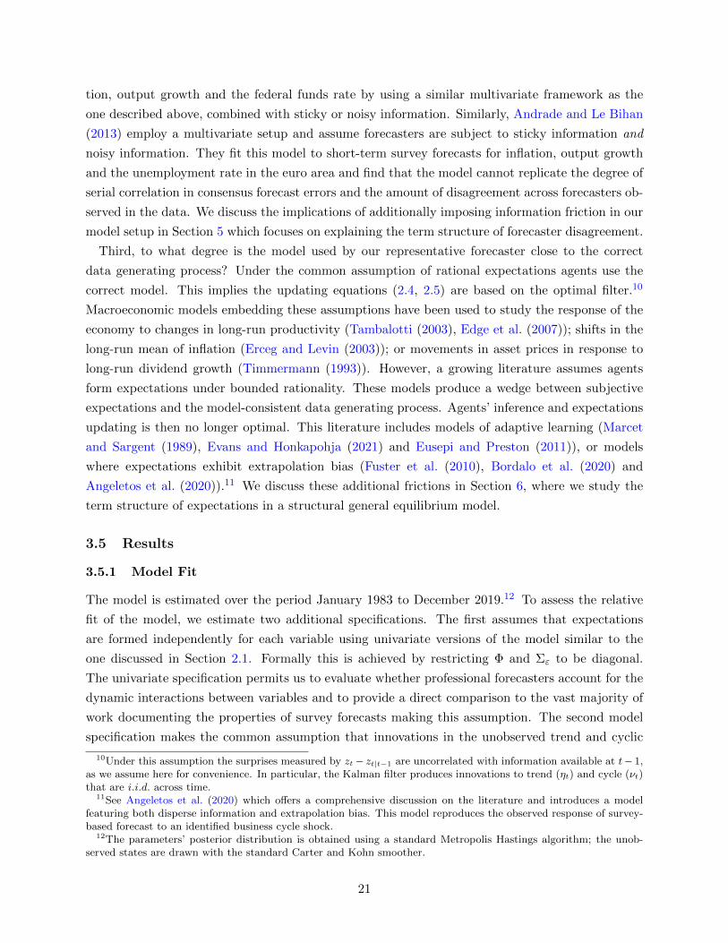
3.5 Results
3.5.1 Model Fit
The model is estimated over the period January 1983 to December 2019.12 To assess the relative
fit of the model, we estimate two additional specifications. The first assumes that expectations
are formed independently for each variable using univariate versions of the model similar to the
one discussed in Section 2.1. Formally this is achieved by restricting Φ and Σε to be diagonal.
The univariate specification permits us to evaluate whether professional forecasters account for the
dynamic interactions between variables and to provide a direct comparison to the vast majority of
work documenting the properties of survey forecasts making this assumption. The second model
specification makes the common assumption that innovations in the unobserved trend and cyclic
10Under this assumption the surprises measured by zt− zt|t−1 are uncorrelated with information available at t− 1,as we assume here for convenience. In particular, the Kalman filter produces innovations to trend (ηt) and cycle (νt)that are i.i.d. across time.
11See Angeletos et al. (2020) which offers a comprehensive discussion on the literature and introduces a modelfeaturing both disperse information and extrapolation bias. This model reproduces the observed response of survey-based forecast to an identified business cycle shock.
12The parameters’ posterior distribution is obtained using a standard Metropolis Hastings algorithm; the unob-served states are drawn with the standard Carter and Kohn smoother.
21

components are independent. By comparing the model fit of the baseline and the restricted spec-
ification, we can then evaluate whether the predicted link between short-term developments and
long-term forecast revisions is consistent with observed survey forecasts.
In terms of marginal likelihood, our baseline specification outperforms the alternative featuring
independent innovations by over 30 log-points, strongly supporting our proposed expectation for-
mation mechanism. The baseline model also dominates (by over 1000 log points!) the alternative
specification where forecasts are modeled independently for each macroeconomic variable.13
Figure 4 sheds further light on the absolute and relative fit of the model by showing a scatter plot
of the fitted values (x-axis) and observed survey data (y-axis) for both the baseline specification (in
red) and the univariate specification (in black). If the model perfectly explained the data with no
observation error, each data point would lie on the forty-five degree line. The baseline model does a
very good job at fitting the 627 times series, especially for the short-term nominal rate. The slightly
worse performance for real GDP and inflation reflects the high volatility in those forecasts at very
short horizons which the model does not fully capture. The fact that this short-term volatility does
not translate to longer-term forecasts suggests it is driven by shocks perceived to be temporary.
The estimation procedure then attributes a large fraction of variation to measurement error because
the model’s innovations affect both short and longer horizons. This short-term volatility problem
does not affect significantly the fit of interest rate forecasts, perhaps because the central bank is
believed to respond to the underlying trend in the economy, rather than to temporary shocks.
Figure 4: Model fit: Baseline vs. univariate model. The figure shows the scatterplot of theprediction error for the baseline model (red) and the univariate specification (black).
(a) Real GDP
-4 -2 0 2 4 6Fitted
-4
-3
-2
-1
0
1
2
3
4
5
6
Sur
vey
For
ecas
t
UnivariateMultivariate
(b) CPI Inflation
-2 0 2 4 6 8Fitted
-2
-1
0
1
2
3
4
5
6
7
8
Sur
vey
For
ecas
t
UnivariateMultivariate
(c) 3-Month T-Bill
0 2 4 6 8 10 12 14Fitted
0
2
4
6
8
10
12
14
Sur
vey
For
ecas
t
UnivariateMultivariate
When comparing our baseline model (red) with the independent forecasts model (black) we see
that the single-equation model performs particularly poorly for forecasts of the short rate. The
much better fit of the multivariate model suggests that market participants form expectations about
the short rate jointly with those of output and inflation. While the difference in fit appears less
striking for inflation and real GDP forecasts, simple measures of forecast performance show that
13In detail, the marginal likelihood for the baseline is 850.13, compared to 818.26 for the model with independentinnovations; and to -1771 for the model with independent univariate forecasts.
22
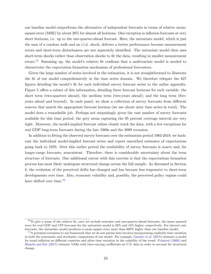
our baseline model outperforms the alternative of independent forecasts in terms of relative mean-
square error (MSE) by about 20% for almost all horizons. One exception is inflation forecasts at very
short horizons, i.e. up to the one-quarter-ahead forecast. Here, the univariate model, which is just
the sum of a random walk and an i.i.d. shock, delivers a better performance because measurement
errors and short-term disturbances are not separately identified. The univariate model then uses
short-term shocks rather than observation shocks to fit the data, resulting in smaller measurement
errors.14 Summing up, the model’s relative fit confirms that a multivariate model is needed to
characterize the expectation formation mechanism of professional forecasters.
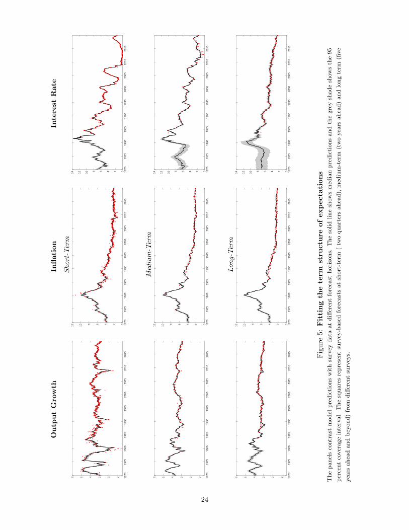
Given the large number of series involved in the estimation, it is not straightforward to illustrate
the fit of our model comprehensively in the time series domain. We therefore relegate the 627
figures detailing the model’s fit for each individual survey forecast series to the online appendix.
Figure 5 offers a subset of this information, detailing three forecast horizons for each variable: the
short term (two-quarters ahead); the medium term (two-years ahead); and the long term (five-
years ahead and beyond). In each panel, we show a collection of survey forecasts from different
sources that match the appropriate forecast horizon (we use about sixty time series in total). The
model does a remarkable job. Perhaps not surprisingly given the vast number of survey forecasts
available for this time period, the grey areas capturing the 95 percent coverage interval are very
tight. Moreover, the model-implied forecast values closely track the data, with a few exceptions for
real GDP long-term forecasts during the late 1980s and the 2009 recession.
In addition to fitting the observed survey forecasts over the estimation period 1983-2019, we back-
cast the individual model-implied forecast series and report smoothed estimates of expectations
going back to 1970. Over this earlier period the availability of survey forecasts is scarce and, for
longer-range forecasts, nonexistent. Therefore, there is considerable uncertainty about the term
structure of forecasts. One additional caveat with this exercise is that the expectations formation
process has most likely undergone structural change across the full sample. As discussed in Section
6, the evolution of the perceived drifts has changed and has become less responsive to short-term
developments over time. Also, economic volatility and, possibly, the perceived policy regime could
have shifted over time.15
14To give a sense of the relative fit, once we exclude nowcasts and one-quarter-ahead forecasts, the mean squarederror for real GDP and CPI forecasts for the univariate model is 22% and 18% higher, respectively. For interest rateforecasts, the univariate model produces a mean square error more than 600% higher than our baseline model.
15A potential extension to our framework that we do not pursue here involves incorporating explicitly time variationin both the systematic and stochastic components of our model. For example, Garnier et al. (2015) estimate a modelfor trend inflation on different countries and allow time variation in the volatility of the trend. Primiceri (2005) andBianchi and Ilut (2017) estimate VARs with time-varying coefficients on U.S. data in order to account for structuralchange.
23
Ou
tpu
tG
row
thIn
flati
on
Inte
rest
Rate
Short
-Ter
m
1970
1975
1980
1985
1990
1995
2000
2005
2010
2015
-202468
1970
1975
1980
1985
1990
1995
2000
2005
2010
2015
02468
1012
1970
1975
1980
1985
1990
1995
2000
2005
2010
2015
02468
101214
Med
ium
-Ter
m
1970
1975
1980
1985
1990
1995
2000
2005
2010
2015
-202468
1970
1975
1980
1985
1990
1995
2000
2005
2010
2015
02468
1012
1970
1975
1980
1985
1990
1995
2000
2005
2010
2015
02468
101214
Lon
g-T
erm
1970
1975
1980
1985
1990
1995
2000
2005
2010
2015
-202468
1970
1975
1980
1985
1990
1995
2000
2005
2010
2015
02468
1012
1970
1975
1980
1985
1990
1995
2000
2005
2010
2015
02468
101214
Fig
ure
5:F
itti
ng
the
term
stru
ctu
reof
exp
ecta
tion
sT
he
panel
sco
ntr
ast
model
pre
dic
tions
wit
hsu
rvey
data
at
diff
eren
tfo
reca
sthori
zons.
The
solid
line
show
sm
edia
npre
dic
tions
and
the
gre
ysh
ade
show
sth
e95
per
cent
cover
age
inte
rval.
The
square
sre
pre
sent
surv
ey-b
ase
dfo
reca
sts
at
short
-ter
m(
two
quart
ers
ahea
d),
med
ium
-ter
m(t
wo
yea
rsahea
d)
and
long
term
(five
yea
rsahea
dand
bey
ond)
from
diff
eren
tsu
rvey
s.
24
These caveats notwithstanding, the model also fits the few observed survey forecasts for output
growth and inflation that are available before 1983 reasonably well. Not surprisingly, the uncertainty
around the estimates increases as we move backwards in time. However, model predictions accord
with conventional wisdom, with an increase in inflation and interest rate expectations over the mid-
1970s, peaking in the early 1980s. While predicted long-term forecasts for real GDP are possibly
too volatile, they capture the higher growth rate during that period. Overall, our simple and
highly parsimonious model fits the term structure of survey-based expectations, especially after the
mid-1980s, exceptionally well.
3.5.2 Evolution of the Term Structure of Expectations
The estimated model allows us to study the implied expected paths of the fitted variables at any
specific point in time. Figure 6 shows a number of “hair charts” which are a convenient way to
summarize the evolution of these forecast paths. The top panel displays real GDP growth; the
middle panels show the nominal interest rate and the underlying rate of CPI inflation;16 and in
the bottom panel we provide the real short-term interest rate computed as the difference between
the nominal short rate and and expected inflation.17 The black solid lines show the actual realized
data while the grey lines show the expected paths of the respective variable over the next ten years
once every twelve months.
16In order to smooth the high volatility in series we plot the model-based measure of CPI which does not transitoryshocks captured by observation errors.
17In particular, since our model is at the monthly frequency we define the real rate as the current interest rate lessthe one-month ahead forecast of inflation.
25

Figure 6: Estimated forecast paths. The figure shows model estimates of survey-based expec-tations up to ten years horizons.
(a) Real GDP Growth
1985 1990 1995 2000 2005 2010 2015 2020 2025 2030-6
-4
-2
0
2
4
6
(b) Short-term Nominal Interest Rate
1985 1990 1995 2000 2005 2010 2015 2020 2025 20300
2
4
6
8
10
12
(c) Inflation
1985 1990 1995 2000 2005 2010 2015 2020 2025 20300
1
2
3
4
5
6
7
(d) Short-term Real Interest Rate
1985 1990 1995 2000 2005 2010 2015 2020 2025 2030-4
-2
0
2
4
6
26
The forecast paths display substantial volatility over time, typically flattening (and often invert-
ing) at the end of economic expansions and steepening in the aftermath of recessions. This pattern
is starker for nominal and real interest rates, as professional forecasters respond to the predictable
component of monetary tightening and easing cycles. For example, the term structure of short rate
expectations inverts in early 1989 when short rates reached their local peak leading into the 1990-91
recession. A flattening and slight inversion is also observed at the end of the 2004–2006 tightening
cycle. Importantly, these estimated measures of short rate expectations based on survey forecasts,
in contrast to many model-based expected short rate paths, are consistent with a perceived zero
lower bound (ZLB) on nominal interest rates. After the short rate reached the ZLB in 2008, the
term structure first flattened and then steepened again as forecasters continued to expect an even-
tual lift-off. This “over-optimism” about lift-off that is apparent in the short rate expectations is
mirrored by over-optimistic real GDP forecasts during the same period.
While expected nominal short rates display a significant degree of volatility, the shape of the
expected path of inflation (third panel) exhibits far less variation, remaining mostly flat around
the prevailing level of inflation. Professional forecasters perceive the persistent component of in-
flation to approximately follow a random walk. An important implication is that movements in
expected nominal short rates translate almost one-to-one to expected real short rates (bottom
panel), consistent with nominal rigidities preventing prices from adjusting in the short term.
The expected ten-year paths of short rates and inflation converge to each variable’s time-varying
long-run mean extracted from all available surveys of professional forecasters. These long-run
projections reflect forecasters’ perceptions of macroeconomic fundamentals rather than cyclical
variation. Long-run forecasts have all varied substantially over the past thirty years. The long-run
expected nominal short rate has gradually fallen from about 8 percent in the mid 1980s to about 2.5
percent in 2019. Much of this decline is accounted for by a secular decline in the expected long-run
level of inflation, which dropped from about 6 percent in the early 1980s to a level of around 2.5
percent in the late 1990s. Since then, the perceived inflation target has remained extremely stable,
only showing a small dip around the Great Recession and over the last two years in our sample.
Using the survey-implied term structures of expectations for the nominal short rate and inflation,
the final panel shows the evolution of the expected real short rate. The long-term expected real
short rate has remained fairly stable around 2 percent over the thirty year period starting in 1983,
but has begun to decline after 2010, falling below 1 percent by the end of 2014. This is consistent
with long-run real GDP growth forecasts which have fallen modestly over the past ten or so years,
reaching slightly below 2 percent by the end of the sample.
3.5.3 Perceived Natural Rate of Interest
The reduction of expected long-run real rates is consistent with recent evidence on the decline of
the natural real rate of interest. Summers (2014), Johannsen and Mertens (2016), Holston et al.
(2017), Del Negro et al. (2018), among others, have argued that long-run equilibrium real rates
in the U.S. have seen a secular decline over the past decades, and dropped suddenly around the
27

financial crisis. A persistently depressed long-run or equilibrium level of the real short rate would
have important implications for macroeconomic analysis. For example, the level of the equilibrium
real short rate is important for assessing the stance of monetary policy. The size of monetary
stimulus is determined by the level of current real interest rates relative to the long-run level.
Given inflation expectations, falling long-run real rates thus imply less nominal space for monetary
policy to respond to an economic contraction.
We compare professional forecasters’ real-time predictions for the long-run value of the real short
rate with two prominent measures of the natural real rate.18 Figure 7 plots our survey-based
measure of the long-run equilibrium real rate (red line) with these alternative estimates. In the
top panel, the solid and dashed black lines show the evolution of the five- and thirty-year forecasts
of the natural rate of interest from the dynamic stochastic general equilibrium model (DSGE) in
Del Negro et al. (2018), updated until the end of our sample. For the period up to 2018, Del Negro
et al. (2018) show that estimates from a Bayesian VAR deliver similar estimates.19
All estimates share a similar broad pattern: the long-run equilibrium real rate fluctuated around
2% until the early 2000s and then started to decline, reaching about 1% by 2012. However, two
differences emerge between our estimate and those implied by the DSGE model. First, the survey-
based estimate fluctuates considerably over the sample reaching below -1% after 1992 and rebound-
ing to nearly 3% in early 2000. In contrast, the DSGE estimates are fairly stable around 2% over
the period 1982-2000. This suggests professional forecasters’ long-run predictions were fairly re-
sponsive to current economic conditions during that period, an issue that we revisit in Section 6.
Second, while the DSGE estimates suggest the estimated long-run natural rate to bottom in 2012
and to begin reverting afterwards, professional forecasters continued to revise their forecasts down-
wards, reaching below -0.5% by the end of 2019. Lastly, the term structure of the DSGE-implied
real short rate forecasts exhibit starkly different behavior across horizons. At the five-year horizon
the natural rate of interest is predicted to be negative until the end of 2017, while the 30-year
forecast predicts above 1.5%. In contrast, survey-based forecasts display almost identical dynamics
for forecast horizons above five years, as movements at such long horizons mimic shifts in the drift
component.
The middle panel in Figure 7 displays the updated estimates of the natural real interest rate
from two versions of the Laubach and Williams (2003) model as the solid and dashed black lines
along with the survey-based expected long-run real short rate as the red solid line. The different
measures broadly co-move but also feature some differences. Most importantly, the natural rate
estimates drop sharply around the financial crisis and have hovered around zero since then, while
professional forecasters long-run expectations have fallen to such low levels only very recently.
Explanations of the secular decline in the real rate include demographic changes, a widespread
productivity slow-down, an increased demand for liquid Treasury securities and other secular shifts
in global savings and investment decisions. Our reduced-form model does not allow us to disentangle
18While we show the forecast for the ten-year forward horizon, we emphasize that the estimated drift looks nearlyidentical. In other words, the survey-based forecast reaches its long-run estimate at horizons around five to ten years.
19Data available at https://github.com/FRBNY-DSGE/rstarBrookings2017.
28
these different explanations. However, use of some basic macroeconomic relationships provides
further insight. Consistent with the Fisher equation, define the perceived long-run real rate as
rt = ωit − ωπt (3.4)
where rt is the long-run estimate of the real short rate and ωit and ωπt are the estimated drifts from
our model, defined in Equation (3.2). Models of long-run economic growth also predict real interest
rates are determined by the rate of time preference and the expected growth rate of output. This
provides the relationship
rt = σ−1ωgt + βt (3.5)
where ωgt , the estimated drift for output growth, proxies expected growth; σ > 0 measures the
intertemporal elasticity of substitution, the sensitivity of expected consumption to changes in the
real interest rate; and βt a residual that captures expected movements in the discount rate, affecting
the equilibrium supply of savings. Combining these two expressions gives a decomposition of real
interest rates
ωit − ωπt = σ−1ωgt + βt. (3.6)
The bottom panel in Figure 7 plots the perceived growth rate of real GDP in the long-run (red
line). It is significantly more volatile than the Laubach and Williams (2003) estimates. Further-
more, consistent with Del Negro et al. (2018), the evolution of long-run expectations of both the
real rate and output growth share a downward trend over the middle part of the sample, suggesting
that expected growth has partially driven the decline in the perceived real rate. This factor plays
less of a role in the estimates of Laubach and Williams (2003). However, the sharp decline of the
expected real rate over the last ten years is unmatched by a decline in expected output growth of a
similar magnitude, suggesting that other factors, captured by the residual βt, explain this decline.
Through a similar decomposition Del Negro et al. (2018) show that rising premiums for the liq-
uidity and safety of Treasury bonds (referred to as the “convenience yield” by Krishnamurthy and
Vissing-Jorgensen (2012)) have been the main drivers of the decline in the estimated natural rate of
interest. We come back to this decomposition in Section 5, when we discuss forecaster disagreement
about long-run interest rates.
29
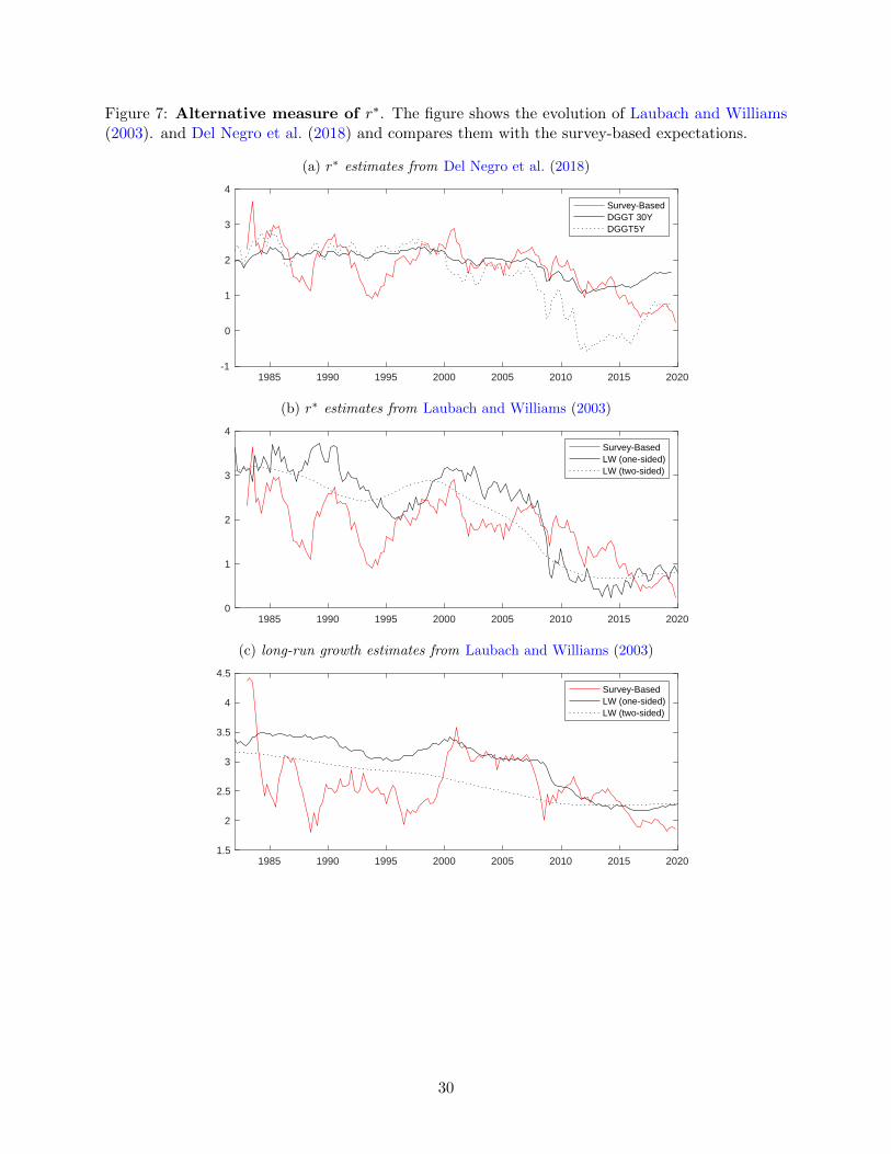
Figure 7: Alternative measure of r∗. The figure shows the evolution of Laubach and Williams(2003). and Del Negro et al. (2018) and compares them with the survey-based expectations.
(a) r∗ estimates from Del Negro et al. (2018)
1985 1990 1995 2000 2005 2010 2015 2020-1
0
1
2
3
4
Survey-BasedDGGT 30YDGGT5Y
(b) r∗ estimates from Laubach and Williams (2003)
1985 1990 1995 2000 2005 2010 2015 20200
1
2
3
4
Survey-BasedLW (one-sided)LW (two-sided)
(c) long-run growth estimates from Laubach and Williams (2003)
1985 1990 1995 2000 2005 2010 2015 20201.5
2
2.5
3
3.5
4
4.5
Survey-BasedLW (one-sided)LW (two-sided)
30

4 Expectations and the Term Structure of Interest Rates
Monetary policy affects the aggregate economy via the term structure of interest rates. While
central banks have tight control over short-term rates, the efficacy of monetary policy depends on
the ability to affect longer-maturity interest rates which drive the saving and investment decisions
of households and firms. Standard macroeconomic models assume that the transmission mechanism
of monetary policy is given by the expectations hypothesis: yields on longer-term government bonds
reflect the average short rate that investors expect to prevail over the life of the bond.
We now use the fitted term structure of expectations to evaluate how well movements in future
short rate expectations explain long-term yields. We do this by decomposing observed government
bond yields into an expectations hypothesis component and a residual component which we interpret
as a measure of the term premium perceived by professional forecasters. The term premium captures
the compensation an investor in longer-term bonds would require for bearing the risk that the
short rate evolves differently than expected. We document that the expectations component fails
to explain the term structure of interest rates for medium to longer-run maturities. Despite sizable
time-series variation, expected short rate paths explain little variation in medium to long-term
Treasury yields. Rather, the term premium explains the bulk of this variation and has a strong
common component across maturities. At the same time, term premiums are only weakly correlated
with the term structure of short rate expectations. These findings suggest that monetary policy –
through its effects on expected future short rates – has imperfect control over the term structure
of interest rates.
4.1 Decomposing The Term Structure of Interest Rates
We obtain zero coupon U.S. Treasury yields from the Gurkaynak et al. (2007) dataset available
on the Board of Governors of the Federal Reserve’s research data page. The sample period is
March 1983–December 2019. Following Fama and Bliss (1987) and Campbell and Shiller (1991),
we decompose Treasury yields into two components: investor expectations about average future
short rates as measured from our model and a residual component which we label the “term
premium.” Because our survey-based term premiums represent the residual between yields and
expected short rates, we can remain agnostic about what specifically they represent. For example,
they might reflect shifts in investor risk attitudes, differences between the expectations of the
marginal investor and consensus expectations, or frictions in the bond market which prevent the
elimination of arbitrage opportunities.
Let yt(n) be the continuously compounded yield on an n-month discount bond and it the risk-free
nominal short rate at time t.20 To separate longer-term from short-term expectations, we conduct
our analyses in terms of forward rates, defined as the current yield of an n-year bond maturing in
n+m years:
ft(n,m) =1
n[(n+m)yt(n+m)−myt(m)]. (4.1)
20The Appendix provides further details on the relevant notation along with specific examples.
31

Because our empirical model of expectations is estimated at a monthly frequency, we construct
annual forward rates as the annual average of monthly forward rates. For example, a 4Y1Y forward
would set n = 12 and m = 48. We then define forward term premiums as the difference between
ft(n,m) and the expected nominal short-term rate over the n months from m months hence, which
we can further decompose into the expected real short rate and expected inflation:
tpfwdt (n,m) = ft(n,m)− 1
n
n+m∑h=m+1
Et [it+h]
= ft(n,m)− 1
n
n+m∑h=m+1
Et [rt+h + πt+h+1] . (4.2)
In other words, the forward term premium is the difference between observed forwards and what
would be the yield predicted by the expectations hypothesis, i.e. the average expected future short
rate over the n months beginning in m months. Note that this is an identity: there are no implicit
assumptions about the rationality or bias of expectations or the data generating process for yields,
expectations, or term premiums.
Figure 8: Forward rates vs. Expected interest rates. The figure shows the evolution ofthe terms structure of forward rates up to then years out (red lines); and the term structure ofexpectations (blue line).
1985 1990 1995 2000 2005 2010 2015 2020 2025 20300
5
10
15
Figure 8 shows the now familiar term structure of nominal short rate expectations (blue line)
discussed in the previous section and superimposes the interest rate path implied by the forward
curve as defined in Equation 4.1 (red line). The latter represents the expected path of short rates
under the pricing (risk-adjusted) measure. The short rate paths implied by the two measures are
quite different. Forward rates imply both a substantially steeper and higher path compared to
our measure of expectations, at least until the early 2000s. Conversely, the forward path becomes
flatter afterwards, while the gap between the end-points of the two measures shrink substantially.
To shed further light on the differences, Figure 9 uses equation 4.2 to decompose nominal Treasury
forward rates into expected future real short rates, expected future inflation, as well as the forward
32
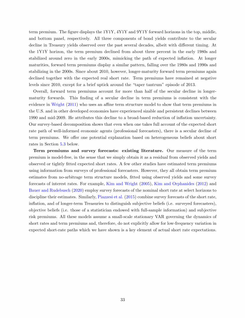
term premium. The figure displays the 1Y1Y, 4Y1Y and 9Y1Y forward horizons in the top, middle,
and bottom panel, respectively. All three components of bond yields contribute to the secular
decline in Treasury yields observed over the past several decades, albeit with different timing. At
the 1Y1Y horizon, the term premium declined from about three percent in the early 1980s and
stabilized around zero in the early 2000s, mimicking the path of expected inflation. At longer
maturities, forward term premiums display a similar pattern, falling over the 1980s and 1990s and
stabilizing in the 2000s. Since about 2010, however, longer-maturity forward term premiums again
declined together with the expected real short rate. Term premiums have remained at negative
levels since 2010, except for a brief uptick around the “taper tantrum” episode of 2013.
Overall, forward term premiums account for more than half of the secular decline in longer-
maturity forwards. This finding of a secular decline in term premiums is consistent with the
evidence in Wright (2011) who uses an affine term structure model to show that term premiums in
the U.S. and in other developed economies have experienced sizable and persistent declines between
1990 and mid-2009. He attributes this decline to a broad-based reduction of inflation uncertainty.
Our survey-based decomposition shows that even when one takes full account of the expected short
rate path of well-informed economic agents (professional forecasters), there is a secular decline of
term premiums. We offer one potential explanation based on heterogeneous beliefs about short
rates in Section 5.3 below.
Term premiums and survey forecasts: existing literature. Our measure of the term
premium is model-free, in the sense that we simply obtain it as a residual from observed yields and
observed or tightly fitted expected short rates. A few other studies have estimated term premiums
using information from surveys of professional forecasters. However, they all obtain term premium
estimates from no-arbitrage term structure models, fitted using observed yields and some survey
forecasts of interest rates. For example, Kim and Wright (2005), Kim and Orphanides (2012) and
Bauer and Rudebusch (2020) employ survey forecasts of the nominal short rate at select horizons to
discipline their estimates. Similarly, Piazzesi et al. (2015) combine survey forecasts of the short rate,
inflation, and of longer-term Treasuries to distinguish subjective beliefs (i.e. surveyed forecasters),
objective beliefs (i.e. those of a statistician endowed with full-sample information) and subjective
risk premiums. All these models assume a small-scale stationary VAR governing the dynamics of
short rates and term premiums and, therefore, do not explicitly allow for low-frequency variation in
expected short-rate paths which we have shown is a key element of actual short rate expectations.
33

Figure 9: The Components of Treasury Forward Rates. These figures show the decom-position of Treasury forwards into the expected short-term real interest rates, expected inflationand the nominal forward term premium. Treasury forwards are (based on) the zero coupon bondyields from the Gurkaynak et al. (2007) dataset available on the Board of Governors of the FederalReserve’s research data page. The sample period is March 1983–September 2016.
(a) 1Y1Y Forward Rate
19821985
19871990
19921995
19972000
20022005
20072010
20122015
20172020
-2
0
2
4
6
Real Exp. Rates Inf Exp. TP
(b) 4Y1Y Forward Rate
19821985
19871990
19921995
19972000
20022005
20072010
20122015
20172020
-2
0
2
4
6
(c) 9Y1Y Forward Rate
19821985
19871990
19921995
19972000
20022005
20072010
20122015
20172020
-2
0
2
4
6
34
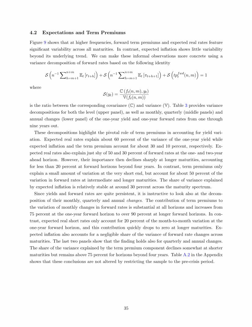
4.2 Expectations and Term Premiums
Figure 9 shows that at higher frequencies, forward term premiums and expected real rates feature
significant variability across all maturities. In contrast, expected inflation shows little variability
beyond its underlying trend. We can make these informal observations more concrete using a
variance decomposition of forward rates based on the following identity
S(n−1
∑n+m
h=m+1Et [rt+h]
)+ S
(n−1
∑n+m
h=m+1Et [πt+h+1]
)+ S
(tpfwdt (n,m)
)= 1
where
S(yt) =C (ft(n,m), yt)
V(ft(n,m))
is the ratio between the corresponding covariance (C) and variance (V). Table 3 provides variance
decompositions for both the level (upper panel), as well as monthly, quarterly (middle panels) and
annual changes (lower panel) of the one-year yield and one-year forward rates from one through
nine years out.
These decompositions highlight the pivotal role of term premiums in accounting for yield vari-
ation. Expected real rates explain about 60 percent of the variance of the one-year yield while
expected inflation and the term premium account for about 30 and 10 percent, respectively. Ex-
pected real rates also explain just shy of 50 and 30 percent of forward rates at the one- and two-year
ahead horizon. However, their importance then declines sharply at longer maturities, accounting
for less than 20 percent at forward horizons beyond four years. In contrast, term premiums only
explain a small amount of variation at the very short end, but account for about 50 percent of the
variation in forward rates at intermediate and longer maturities. The share of variance explained
by expected inflation is relatively stable at around 30 percent across the maturity spectrum.
Since yields and forward rates are quite persistent, it is instructive to look also at the decom-
position of their monthly, quarterly and annual changes. The contribution of term premiums to
the variation of monthly changes in forward rates is substantial at all horizons and increases from
75 percent at the one-year forward horizon to over 90 percent at longer forward horizons. In con-
trast, expected real short rates only account for 20 percent of the month-to-month variation at the
one-year forward horizon, and this contribution quickly drops to zero at longer maturities. Ex-
pected inflation also accounts for a negligible share of the variance of forward rate changes across
maturities. The last two panels show that the finding holds also for quarterly and annual changes.
The share of the variance explained by the term premium component declines somewhat at shorter
maturities but remains above 75 percent for horizons beyond four years. Table A.2 in the Appendix
shows that these conclusions are not altered by restricting the sample to the pre-crisis period.
35

Table 3: Variance Decompositions for Yield Components
This table presents variance decompositions for the one-year yield and one-year forward rates ranging from one though
ten-years out. For each maturity, the numbers shown represent the ratio of the covariance of the respective forward
with its individual components (average expected real short rate, average expected inflation, and term premium)
divided by the variance of the forward. The top panel provides variance decompositions for forward rates in levels,
and the following panels the 1-month, 3-month and 12-month change in forward rates. The sample period is March
1983–December 2019.
Y1 1Y1Y 2Y1Y 3Y1Y 4Y1Y 5Y1Y 6Y1Y 7Y1Y 8Y1Y 9Y1Y
LevelsAvg Exp Nominal SR 0.90 0.76 0.64 0.55 0.50 0.48 0.47 0.48 0.49 0.50
Avg Exp Real SR 0.61 0.47 0.34 0.25 0.19 0.17 0.16 0.16 0.17 0.18Avg Exp Inflation 0.30 0.29 0.29 0.30 0.30 0.31 0.31 0.32 0.32 0.32
Fwd Term Premium 0.10 0.24 0.36 0.45 0.50 0.52 0.53 0.52 0.51 0.501-Month Changes
Avg Exp Nominal SR 0.61 0.28 0.14 0.09 0.07 0.06 0.05 0.04 0.04 0.04Avg Exp Real SR 0.49 0.22 0.10 0.06 0.03 0.02 0.01 -0.00 -0.01 -0.01Avg Exp Inflation 0.11 0.06 0.04 0.04 0.04 0.04 0.04 0.05 0.05 0.05
Fwd Term Premium 0.39 0.72 0.86 0.91 0.93 0.94 0.95 0.96 0.96 0.963-Month Changes
Avg Exp Nominal SR 0.79 0.43 0.26 0.18 0.14 0.11 0.09 0.08 0.07 0.07Avg Exp Real SR 0.64 0.34 0.19 0.11 0.07 0.04 0.02 0.00 -0.01 -0.01Avg Exp Inflation 0.15 0.09 0.07 0.07 0.07 0.07 0.08 0.08 0.08 0.08
Fwd Term Premium 0.21 0.57 0.74 0.82 0.86 0.89 0.91 0.92 0.93 0.9312-Month Changes
Avg Exp Nominal SR 0.92 0.71 0.50 0.34 0.24 0.19 0.15 0.13 0.12 0.12Avg Exp Real SR 0.75 0.55 0.36 0.22 0.12 0.07 0.03 0.01 -0.00 -0.01Avg Exp Inflation 0.17 0.15 0.14 0.13 0.12 0.12 0.12 0.12 0.12 0.13
Fwd Term Premium 0.08 0.29 0.50 0.66 0.76 0.81 0.85 0.87 0.88 0.88
Figure 10: Term Structures of Expectations and Forwards. These figures show differentaspects of the term structure of various second moments of forward expectations and forward rates.The top left panel displays the relative standard deviation of changes in expectations compared tochanges in forward rates by forward maturity. The top right panel shows the correlation coefficientbetween changes in expectations compared to changes in forward rates by forward maturity. Theblack solid line denotes 1-month changes whereas the dotted line denotes 12-month changes.
(a) Relative Vol. of Expectations wrt Forwards
1Y1Y 2Y1Y 3Y1Y 4Y1Y 5Y1Y 6Y1Y 7Y1Y 8Y1Y 9Y1Y0
0.1
0.2
0.3
0.4
0.5
0.6
0.7
0.8
0.9
1
1-Month Change
12-Month Change
(b) Corr. b/t Expectations & Forwards
1Y1Y 2Y1Y 3Y1Y 4Y1Y 5Y1Y 6Y1Y 7Y1Y 8Y1Y 9Y1Y0
0.1
0.2
0.3
0.4
0.5
0.6
0.7
0.8
0.9
1
1-Month Change
12-Month Change
Co-movement across time. Given the considerable volatility of expected short rates, how can
we explain the prominent role of term premiums in accounting for the variability of longer-maturity
bond yields? Figure 10 sheds light on this question. The left-hand chart reiterates that nominal
36
rate expectations are fairly volatile at all forecast horizons when compared to actual forward rates:
at horizons beyond three years, their volatility ranges from over 40% for 12-month changes to 50%
for monthly changes. However, the right-hand chart shows that changes in expectations co-move
very little with changes in yields, except at short forecast horizons. Since the variance share of the
yield components (S) can be re-expressed in terms of variances and correlations
S (yt) = Corr (ft(n,m), yt) ·(
V(yt)
V(ft(n,m)
)1/2
,
the low shares of variance explained by real rate and inflation expectations must be due to the fact
that expectations are only weakly correlated with forward yields. This is consistent with aggregate
shocks affecting the components of the yield curve in different ways.21
21Note that the importance of term premiums for variations in Treasury yields is not driven by the recent financialcrisis and the large-scale asset purchases undertaken by the Federal Reserve. When repeating the variance decom-positions ending the sample in 2007, we find that term premiums played an even larger role before the financialcrisis.
37

Figure 11: Short Rate Forecast errors vs. Changes in LR Forecasts. This figure comparesforecast errors with changes in long-run objects. Nominal and real short-rate forecast errors arecalculated as the backward-looking 12-month cumulative sum of monthly forecast errors. Revisionsto long-run forecasts and changes in term premiums are defined as changes relative to 12 monthsago. The sample period is January 1984–December 2019.
(a) Nominal short rate forecast Errors vs. Revisions in Long-run (9Y1Y) Forecasts
1985 1990 1995 2000 2005 2010 2015 2020-20
-10
0
10
20
-1.5
-1
-0.5
0
0.5
1
Forecast Errors Changes in LR Forecasts
(b) Real short rate forecast errors vs. Revisions in Long-run (9Y1Y) Forecasts
1985 1990 1995 2000 2005 2010 2015 2020-20
-10
0
10
20
-2
-1
0
1
2
Forecast Errors Changes in LR Forecasts
(c) Nominal short rate forecast errors vs. Changes in the 9Y1Y Term premium
1985 1990 1995 2000 2005 2010 2015 2020-20
-10
0
10
20
-4
-2
0
2
4
Forecast Errors Changes in LR Term Premium
38
To gain further intuition about the determinants of the longer-term interest rates we return to
the simple model of Section 2.1. Revisions in long-term expectations should be positively related
to short-term forecast errors. The two top panels in Figure 11 show this is indeed the case for both
nominal and real interest rates. The in-sample correlation is 58% and 43% for nominal and real
short rates. This implies that market participants update their views about the long-term mean of
the nominal and real short rate in response to new information captured by forecast surprises. The
bottom panel that shows the correlation between short-term forecast revisions and our measure
of the term premium tells a different story. A correlation of only -9% suggests that other forces
determine interest rate term premiums.
Co-movement in the cross-section. We have discussed the weak co-movement of expected
short rates and forward rates in the time dimension. Next, we uncover another important difference
by looking across bond maturities. A long literature in finance has documented that government
bond yields feature substantial co-movement across maturities (e.g., Garbade 1996, Scheinkman
and Litterman 1991). This is also true in our sample: the first two principal components extracted
from the ten maturities shown in Table 3 explain 97 and 3 percent of their joint variation. The
loadings of these principal components confirm the common interpretation as level and slope of the
yield curve.
Based on our decomposition of forwards into expected short rate and term premium components,
we can parse out the sources of the strong cross-sectional correlation. In line with the results in Table
3, almost half of the variance of the level factor is explained by term premiums, one third by expected
inflation and the remaining 20 percent by expected real short rates. Also consistent with the
variance decompositions for individual forwards, almost 90 percent of the month-to-month variation
in the level factor and more than three quarters of the year-over-year variation are explained by term
premiums. The expectations components are somewhat more important for the slope factor: 85
percent of its variation is accounted for by expected real short rates, about 10 percent by expected
inflation and the remainder by term premiums. However, more than two thirds of the month-to-
month variation of the slope factor is explained by term premiums, in line with the above finding
that only a small share of the yield curve variation at higher frequencies is driven by expectations.
39

Figure 12: Co-Movement of Expected Rates and Term Premiums. These figures show12-month changes in forward rates (top chart), expected forward nominal short-term rates (mid-dle chart) and the forward term premium (bottom chart). The sample period is January 1984–December 2019.
(a) Forward Rates
19821985
19871990
19921995
19972000
20022005
20072010
20122015
20172020
-4
-3
-2
-1
0
1
2
3
1Y1Y Fwd 9Y1Y Fwd
(b) Expected Forward Rates
19821985
19871990
19921995
19972000
20022005
20072010
20122015
20172020
-4
-3
-2
-1
0
1
2
3
(c) Forward Term Premiums
19821985
19871990
19921995
19972000
20022005
20072010
20122015
20172020
-4
-3
-2
-1
0
1
2
3
Figure 12 visualizes the importance of term premiums for the strong co-movement across maturi-
ties. It shows twelve-month changes in short and long-maturity forward rates (top panel), expected
rates (middle panel), and forward term premiums (bottom panel) for the 1Y1Y and 9Y1Y forward
maturities. The figure documents that across maturities survey-based term premiums co-move
much more strongly than survey-based expected future short rates, or forwards themselves. Twelve
40
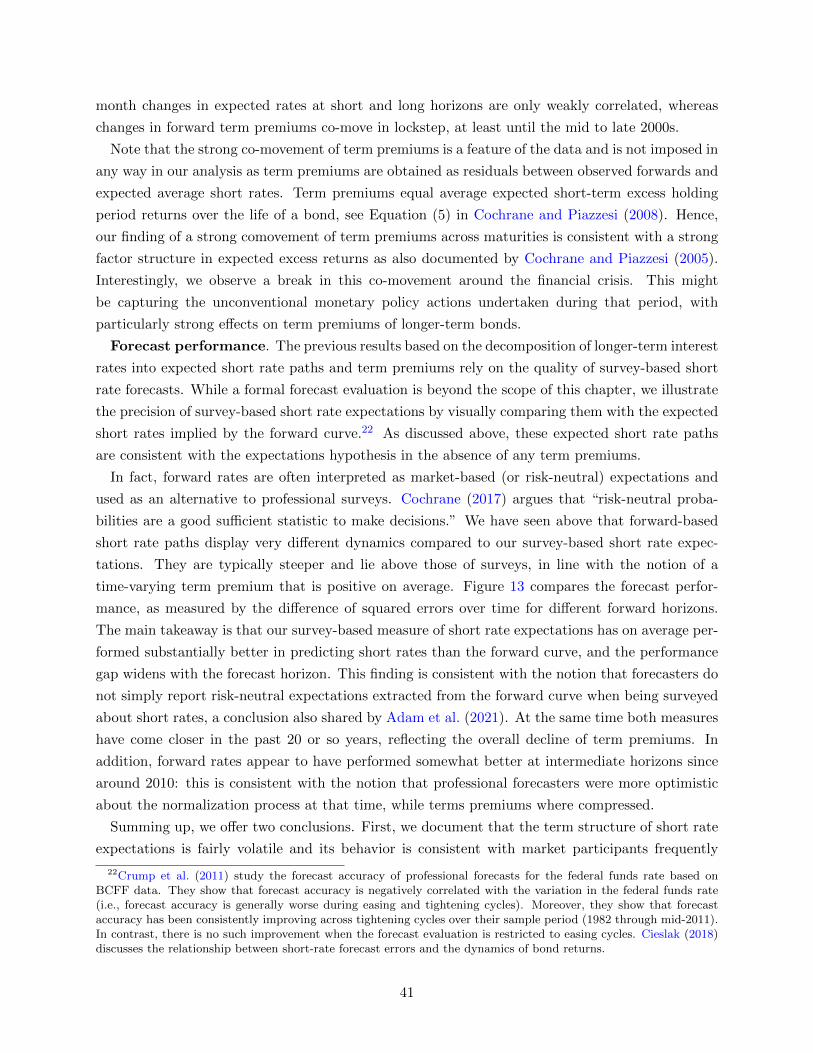
month changes in expected rates at short and long horizons are only weakly correlated, whereas
changes in forward term premiums co-move in lockstep, at least until the mid to late 2000s.
Note that the strong co-movement of term premiums is a feature of the data and is not imposed in
any way in our analysis as term premiums are obtained as residuals between observed forwards and
expected average short rates. Term premiums equal average expected short-term excess holding
period returns over the life of a bond, see Equation (5) in Cochrane and Piazzesi (2008). Hence,
our finding of a strong comovement of term premiums across maturities is consistent with a strong
factor structure in expected excess returns as also documented by Cochrane and Piazzesi (2005).
Interestingly, we observe a break in this co-movement around the financial crisis. This might
be capturing the unconventional monetary policy actions undertaken during that period, with
particularly strong effects on term premiums of longer-term bonds.
Forecast performance. The previous results based on the decomposition of longer-term interest
rates into expected short rate paths and term premiums rely on the quality of survey-based short
rate forecasts. While a formal forecast evaluation is beyond the scope of this chapter, we illustrate
the precision of survey-based short rate expectations by visually comparing them with the expected
short rates implied by the forward curve.22 As discussed above, these expected short rate paths
are consistent with the expectations hypothesis in the absence of any term premiums.
In fact, forward rates are often interpreted as market-based (or risk-neutral) expectations and
used as an alternative to professional surveys. Cochrane (2017) argues that “risk-neutral proba-
bilities are a good sufficient statistic to make decisions.” We have seen above that forward-based
short rate paths display very different dynamics compared to our survey-based short rate expec-
tations. They are typically steeper and lie above those of surveys, in line with the notion of a
time-varying term premium that is positive on average. Figure 13 compares the forecast perfor-
mance, as measured by the difference of squared errors over time for different forward horizons.
The main takeaway is that our survey-based measure of short rate expectations has on average per-
formed substantially better in predicting short rates than the forward curve, and the performance
gap widens with the forecast horizon. This finding is consistent with the notion that forecasters do
not simply report risk-neutral expectations extracted from the forward curve when being surveyed
about short rates, a conclusion also shared by Adam et al. (2021). At the same time both measures
have come closer in the past 20 or so years, reflecting the overall decline of term premiums. In
addition, forward rates appear to have performed somewhat better at intermediate horizons since
around 2010: this is consistent with the notion that professional forecasters were more optimistic
about the normalization process at that time, while terms premiums where compressed.
Summing up, we offer two conclusions. First, we document that the term structure of short rate
expectations is fairly volatile and its behavior is consistent with market participants frequently
22Crump et al. (2011) study the forecast accuracy of professional forecasts for the federal funds rate based onBCFF data. They show that forecast accuracy is negatively correlated with the variation in the federal funds rate(i.e., forecast accuracy is generally worse during easing and tightening cycles). Moreover, they show that forecastaccuracy has been consistently improving across tightening cycles over their sample period (1982 through mid-2011).In contrast, there is no such improvement when the forecast evaluation is restricted to easing cycles. Cieslak (2018)discusses the relationship between short-rate forecast errors and the dynamics of bond returns.
41

updating their beliefs about the medium- to long-term evolution of the policy rate. Second, we
show that the term structure of interest rates is only partly driven by short rate expectations. The
residual component, the term premium, plays a key role in determining the equilibrium evolution
of interest rates at longer maturities. This component is often left unaccounted for in standard
macroeconomic models used for monetary policy analysis. In the next section, we argue that
disagreement among forecasters about the long-run mean of the short rate can partly explain the
secular decline of term premiums documented here and in previous work.
Figure 13: Forecast errors. This figure shows the difference between the mean-square forecasterror (MSFE) of survey expectations less the MSFE of market expectations. Values below zeroindicate that survey expectations have a lower MSFE. The sample period is January 1983–December2019.
(a) 1Y Rate
1980 1985 1990 1995 2000 2005 2010 2015 2020-8
-6
-4
-2
0
2
Survey Exp. Error less Market Exp. Error
(b) 1Y1Y Forward Rate
1980 1985 1990 1995 2000 2005 2010 2015 2020-30
-20
-10
0
10
(c) 4Y1Y Forward Rate
1980 1985 1990 1995 2000 2005 2010 2015 2020-40
-30
-20
-10
0
10
(d) 5Y5Y Forward Rate
1980 1985 1990 1995 2000 2005 2010 2015 2020
-60
-40
-20
0
(e) 9Y1Y Forward Rate
1980 1985 1990 1995 2000 2005 2010 2015 2020-80
-60
-40
-20
0
42

5 The Term Structure of Disagreement
Throughout the paper we have focused on a consensus measure of expectations. While this term
structure of expectations can be enormously useful in many economic applications, it neglects the
dispersion in individual forecasts that has been widely documented for professional forecasters,
households, firms and policymakers. A growing literature studies the implications of this empirical
observation for macroeconomics and finance.23 In this section, we document substantial disagree-
ment about the expected nominal short rate path, particularly in the long-run. We show that
the term structure of disagreement of short rates starkly differs from that observed for output
and inflation and discuss a modeling framework that can explain these differences. We then use
this framework to study the determinants of short rate disagreement. Finally, we link short rate
disagreement to the evolution of term premiums in a heterogeneous agent term structure model.
Along the way, we selectively review the literature on forecast disagreement.
5.1 Disagreement About the Short Rate, Real Output Growth, and Inflation
We now document some basic facts about the term structure of disagreement using the Blue Chip
Financial Forecasts (BCFF) survey. A strength of this data-set is that it contains forecasts at very
different horizons, from one-quarter ahead to ten-years ahead. This provides a clear picture of the
term structure of expectations over a long sample. While it does not provide the full distribution of
survey responses at medium to long horizons, the BCFF reports the average of the top and bottom
deciles of all respondents at these longer horizons.
Andrade et al. (2016) propose using the difference between the average response of the top and
bottom deciles of forecasters as a measure of disagreement. They show that at shorter forecast
horizons for which the full distribution of individual forecasts is available, this measure is strongly
correlated with other commonly used measures of forecast dispersion such as the cross-sectional
standard deviation or the interquartile range. Figure 14 reproduces some stylized facts from An-
drade et al. (2016). The left panel shows the term structure of disagreement. That is the average
disagreement at each forecasting horizon. The nature of disagreement is fundamentally different
across macroeconomic variables: the term structure of disagreement is upward-sloping only for
short rate forecasts while it is flat across horizons for inflation and downward-sloping for output
growth. The right panel shows the time series of disagreement at long horizons for output, inflation
and the short-term interest rate. Evident are both cycle and trend components, which differ across
variables.
23For a review of the literature see Angeletos et al. (2020), Andrade et al. (2016) and references therein.
43
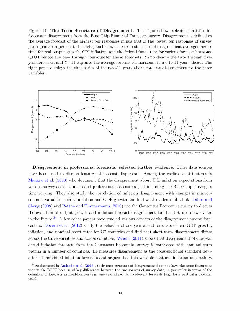
Figure 14: The Term Structure of Disagreement. This figure shows selected statistics forforecaster disagreement from the Blue Chip Financial Forecasts survey. Disagreement is defined asthe average forecast of the highest ten responses minus that of the lowest ten responses of surveyparticipants (in percent). The left panel shows the term structure of disagreement averaged acrosstime for real output growth, CPI inflation, and the federal funds rate for various forecast horizons.Q1Q4 denote the one- through four-quarter ahead forecasts, Y2Y5 denote the two- through five-year forecasts, and Y6-11 captures the average forecast for horizons from 6-to-11 years ahead. Theright panel displays the time series of the 6-to-11 years ahead forecast disagreement for the threevariables.
Q1 Q2 Q3 Q4 Y2 Y3 Y4 Y5 Y6-11
Forecast Horizon
0
0.5
1
1.5
2
2.5
3
Dis
agre
emen
t (pe
rcen
t)
OutputInflationFederal Funds Rate
1987 1990 1992 1995 1997 2000 2002 2005 2007 2010 20120
0.5
1
1.5
2
2.5
3
3.5
4
Dis
agre
emen
t (pe
rcen
t)
OutputInflationFederal Funds Rate
Figure 1: This figure shows selected statistics for forecaster disagreement from the Blue Chip Finan-cial Forecasts survey. Disagreement is defined as the average forecast of the highest ten responsesminus that of the lowest ten responses of survey participants (in percent). The left panel showsthe term structure of disagreement averaged across time for real output growth, CPI inflation, andthe federal funds rate for various forecast horizons. Q1–Q4 denote the one- through four-quarterahead forecasts, Y2–Y5 denote the two- through five-year forecasts, and Y6-11 captures the aver-age forecast for horizons from 6-to-11 years ahead. The right panel displays the time series of the6-to-11 years ahead forecast disagreement for the three variables.
Disagreement in professional forecasts: selected further evidence. Other data sources
have been used to discuss features of forecast dispersion. Among the earliest contributions is
Mankiw et al. (2003) who document that the disagreement about U.S. inflation expectations from
various surveys of consumers and professional forecasters (not including the Blue Chip survey) is
time varying. They also study the correlation of inflation disagreement with changes in macroe-
conomic variables such as inflation and GDP growth and find weak evidence of a link. Lahiri and
Sheng (2008) and Patton and Timmermann (2010) use the Consensus Economics survey to discuss
the evolution of output growth and inflation forecast disagreement for the U.S. up to two years
in the future.24 A few other papers have studied various aspects of the disagreement among fore-
casters. Dovern et al. (2012) study the behavior of one-year ahead forecasts of real GDP growth,
inflation, and nominal short rates for G7 countries and find that short-term disagreement differs
across the three variables and across countries. Wright (2011) shows that disagreement of one-year
ahead inflation forecasts from the Consensus Economics survey is correlated with nominal term
premia in a number of countries. He measures disagreement as the cross-sectional standard devi-
ation of individual inflation forecasts and argues that this variable captures inflation uncertainty.
24As discussed in Andrade et al. (2016), their term structure of disagreement does not have the same features asthat in the BCFF because of key differences between the two sources of survey data, in particular in terms of thedefinition of forecasts as fixed-horizon (e.g. one year ahead) or fixed-event forecasts (e.g. for a particular calendaryear).
44

Using data on individual point as well as density forecasts from the U.S. Survey of Professional
Forecasters, Zarnowitz and Lambros (1987) study the relationship between consensus forecasts and
measures of uncertainty while Rich and Tracy (2010) show that disagreement about U.S. inflation
is not systematically related to measures of inflation uncertainty. Lastly, Boero et al. (2008) study
the relation between forecast uncertainty and disagreement up to two years into the future for a
UK survey of professional forecasts and find a sustained reduction of inflation uncertainty after the
introduction of a formal inflation targeting regime by the Bank of England.
5.2 What Drives Disagreement About the Short Rate?
Section 3.5.3 showed the secular trend in long-run forecasts of the nominal and real short rate and
discussed some potential factors behind this decline. Here we provide a similar investigation of the
drivers of long-run disagreement about the short rate. Consistent with the treatment of consen-
sus expectations, forecasters must disentangle slow-moving changes from short-term fluctuations.
Following Andrade et al. (2016), each individual forecaster has imperfect information about the
current state of the economy because they only infrequently update their information set; this is
an economy with sticky information similar to Mankiw and Reis (2002).25
In terms of the model outlined in Section 3.1, at any point in time individual forecasters see only
a subset of new observations about the three variables in the vector zt = ( gt πt it )′ with a
constant probability.26 This implies the Kalman filter involves a time-varying observation equation
z(j)t = h
(j)t
(xtωt
)where z
(j)t denotes the subset of variables observed by forecaster j in period t, and xt and ωt are
the unobserved cycle and trend components. The dimension of the observation matrix h(j)t changes
across agents and across time depending on which elements of zt are observed. At any point in
time only a fraction of agents will observe a particular element of zt. When agents do not observe
the full vector zt they use the Kalman filter with missing observations. Updating of the unobserved
trend component in this model is then captured by the following recursion
ω(j)t = ω
(j)t−1 + κ
(j)ω,t ×
(z
(j)t − z
(j)t|t−1
)where κ
(j)ω,t denotes the time-varying Kalman gain that changes size with z
(j)t . These assumptions
deliver dispersed forecasts at all forecast horizons because agents observe a different slice of available
information at any point in time.
Calibrated to survey forecasts of realized output growth, inflation and the nominal short rate,
the model replicates closely the term structure of disagreement observed in the data. Importantly,
Andrade et al. (2016) show that the combination of sticky information and the trend-cycle infer-
25Andrade et al. (2016) show that an information friction where agents only observe noisy signals of the truevariables they intend to predict (Sims (2003) or Woodford (2003a)) yields similar results.
26This probability is allowed to be different across variables.
45
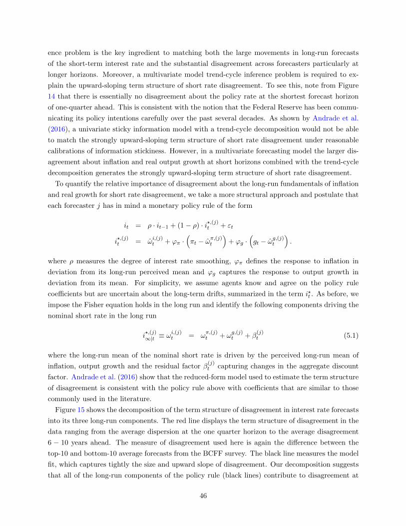
ence problem is the key ingredient to matching both the large movements in long-run forecasts
of the short-term interest rate and the substantial disagreement across forecasters particularly at
longer horizons. Moreover, a multivariate model trend-cycle inference problem is required to ex-
plain the upward-sloping term structure of short rate disagreement. To see this, note from Figure
14 that there is essentially no disagreement about the policy rate at the shortest forecast horizon
of one-quarter ahead. This is consistent with the notion that the Federal Reserve has been commu-
nicating its policy intentions carefully over the past several decades. As shown by Andrade et al.
(2016), a univariate sticky information model with a trend-cycle decomposition would not be able
to match the strongly upward-sloping term structure of short rate disagreement under reasonable
calibrations of information stickiness. However, in a multivariate forecasting model the larger dis-
agreement about inflation and real output growth at short horizons combined with the trend-cycle
decomposition generates the strongly upward-sloping term structure of short rate disagreement.
To quantify the relative importance of disagreement about the long-run fundamentals of inflation
and real growth for short rate disagreement, we take a more structural approach and postulate that
each forecaster j has in mind a monetary policy rule of the form
it = ρ · it−1 + (1− ρ) · i?,(j)t + εt
i?,(j)t = ω
i,(j)t + ϕπ ·
(πt − ωπ,(j)t
)+ ϕg ·
(gt − ωg,(j)t
).
where ρ measures the degree of interest rate smoothing, ϕπ defines the response to inflation in
deviation from its long-run perceived mean and ϕg captures the response to output growth in
deviation from its mean. For simplicity, we assume agents know and agree on the policy rule
coefficients but are uncertain about the long-term drifts, summarized in the term i?t . As before, we
impose the Fisher equation holds in the long run and identify the following components driving the
nominal short rate in the long run
i?,(j)∞|t ≡ ω
i,(j)t = ω
π,(j)t + ω
g,(j)t + β
(j)t (5.1)
where the long-run mean of the nominal short rate is driven by the perceived long-run mean of
inflation, output growth and the residual factor β(j)t capturing changes in the aggregate discount
factor. Andrade et al. (2016) show that the reduced-form model used to estimate the term structure
of disagreement is consistent with the policy rule above with coefficients that are similar to those
commonly used in the literature.
Figure 15 shows the decomposition of the term structure of disagreement in interest rate forecasts
into its three long-run components. The red line displays the term structure of disagreement in the
data ranging from the average dispersion at the one quarter horizon to the average disagreement
6 − 10 years ahead. The measure of disagreement used here is again the difference between the
top-10 and bottom-10 average forecasts from the BCFF survey. The black line measures the model
fit, which captures tightly the size and upward slope of disagreement. Our decomposition suggests
that all of the long-run components of the policy rule (black lines) contribute to disagreement at
46
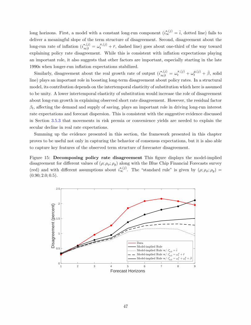
long horizons. First, a model with a constant long-run component (i?,(j)∞ = i, dotted line) fails to
deliver a meaningful slope of the term structure of disagreement. Second, disagreement about the
long-run rate of inflation (i?,(j)∞|t = ω
π,(j)t + r, dashed line) goes about one-third of the way toward
explaining policy rate disagreement. While this is consistent with inflation expectations playing
an important role, it also suggests that other factors are important, especially starting in the late
1990s when longer-run inflation expectations stabilized.
Similarly, disagreement about the real growth rate of output (i?,(j)∞|t = ω
π,(j)t + ω
g,(j)t + β, solid
line) plays an important role in boosting long-term disagreement about policy rates. In a structural
model, its contribution depends on the intertemporal elasticity of substitution which here is assumed
to be unity. A lower intertemporal elasticity of substitution would increase the role of disagreement
about long-run growth in explaining observed short rate disagreement. However, the residual factor
βt, affecting the demand and supply of saving, plays an important role in driving long-run interest
rate expectations and forecast dispersion. This is consistent with the suggestive evidence discussed
in Section 3.5.3 that movements in risk premia or convenience yields are needed to explain the
secular decline in real rate expectations.
Summing up the evidence presented in this section, the framework presented in this chapter
proves to be useful not only in capturing the behavior of consensus expectations, but it is also able
to capture key features of the observed term structure of forecaster disagreement.
Figure 15: Decomposing policy rate disagreement This figure displays the model-implieddisagreement for different values of (ρ; ρφ; ρg) along with the Blue Chip Financial Forecasts survey
(red) and with different assumptions about i?,(j)∞ . The “standard rule” is given by (ρ; ρφ; ρg) =
(0.90; 2.0; 0.5).
1 2 3 4 5 6 7 8 9
Forecast Horizons
0
0.5
1
1.5
2
2.5
Dis
agre
emen
t (pe
rcen
t)
47

5.3 Interest Rate Disagreement and the Term Premium
In Section 4 we showed that while revisions of long-term policy rate forecasts are strongly correlated
with short-term forecast errors of the short rate, changes in the term premium, measured as the
difference between observed yields and survey-based consensus forecasts of the short rate, are
essentially uncorrelated with these short-term forecast errors. Here we explore the link between
the term premium and forecast dispersion about policy rates. Figure 16 plots the ten-year term
premium along with the difference between the top-10 and the bottom-10 average forecasts of
the federal funds rate from the BCFF survey for two horizons: five years ahead and 7-11 years
ahead. The chart shows a strong correlation between the consensus term premium and short rate
disagreement. Both have been declining over the past three decades, but have also been comoving
at higher frequencies. This evidence is suggestive of a link between market-wide measures of risk
premiums and short rate disagreement.
Figure 16: Term premiums and short rate disagreement. This chart shows the 5-year/5-yearforward Treasury term premium together with a measure of policy rate disagreement at similarhorizons. Disagreement is measured as the difference between the top-10 and bottom-10 averageforecasts of the 3-month T-bill at the five-year or six-year ahead (“Y6”) and 6-10 or 7-11 yearsahead (“Y7-11”) horizons from the Blue Chip Financial Forecasts survey.
19801982
19851987
19901992
19951997
20002002
20052007
20102012
20152017
2020-2
0
2
4
6
8
0
1
2
3
4
5
5Y5Y Forward Term Premium (left) Y6 (right) Y7-11 (right)
While the traditional approach to modeling the term structure of interest rates, both in structural
and reduced-form models, relies on a representative agent formulation, a recent literature has made
progress incorporating beliefs heterogeneity in asset pricing models. In general, in this literature
heterogeneity drives a wedge between the marginal and average investor, with implications for
asset prices. As shown by Jouini and Napp (2007) and Bhamra and Uppal (2014), among others,
in models with heterogeneous beliefs investors with a higher share of the total wealth have a
greater impact on the marginal valuation of risky assets. Xiong and Yan (2010) apply this idea to
a model of bond pricing. Consider an econometrician measuring an aggregate term premium in a
48
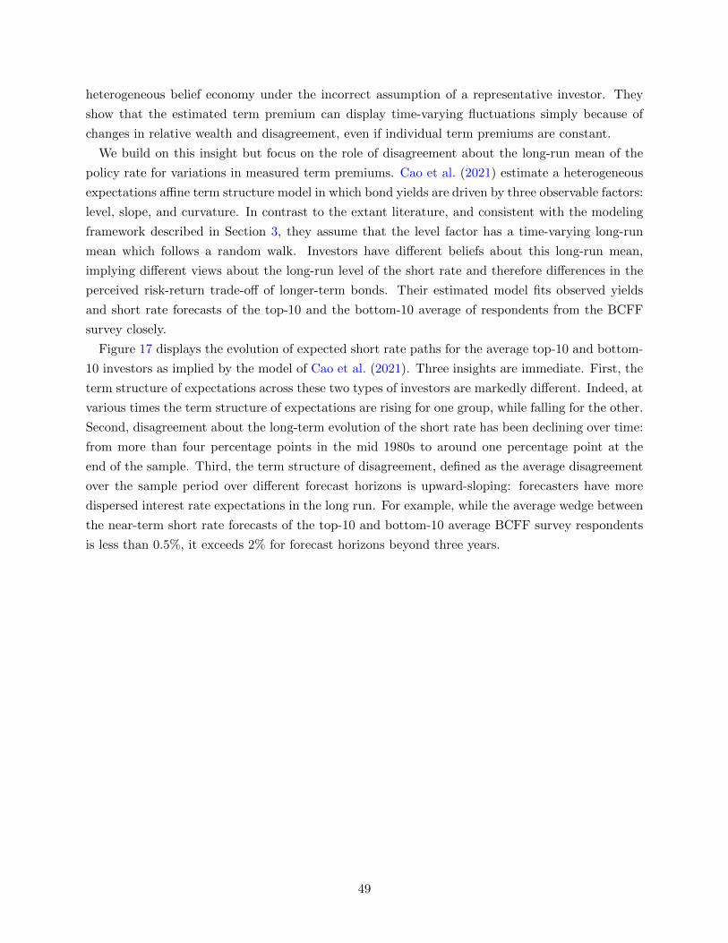
heterogeneous belief economy under the incorrect assumption of a representative investor. They
show that the estimated term premium can display time-varying fluctuations simply because of
changes in relative wealth and disagreement, even if individual term premiums are constant.
We build on this insight but focus on the role of disagreement about the long-run mean of the
policy rate for variations in measured term premiums. Cao et al. (2021) estimate a heterogeneous
expectations affine term structure model in which bond yields are driven by three observable factors:
level, slope, and curvature. In contrast to the extant literature, and consistent with the modeling
framework described in Section 3, they assume that the level factor has a time-varying long-run
mean which follows a random walk. Investors have different beliefs about this long-run mean,
implying different views about the long-run level of the short rate and therefore differences in the
perceived risk-return trade-off of longer-term bonds. Their estimated model fits observed yields
and short rate forecasts of the top-10 and the bottom-10 average of respondents from the BCFF
survey closely.
Figure 17 displays the evolution of expected short rate paths for the average top-10 and bottom-
10 investors as implied by the model of Cao et al. (2021). Three insights are immediate. First, the
term structure of expectations across these two types of investors are markedly different. Indeed, at
various times the term structure of expectations are rising for one group, while falling for the other.
Second, disagreement about the long-term evolution of the short rate has been declining over time:
from more than four percentage points in the mid 1980s to around one percentage point at the
end of the sample. Third, the term structure of disagreement, defined as the average disagreement
over the sample period over different forecast horizons is upward-sloping: forecasters have more
dispersed interest rate expectations in the long run. For example, while the average wedge between
the near-term short rate forecasts of the top-10 and bottom-10 average BCFF survey respondents
is less than 0.5%, it exceeds 2% for forecast horizons beyond three years.
49
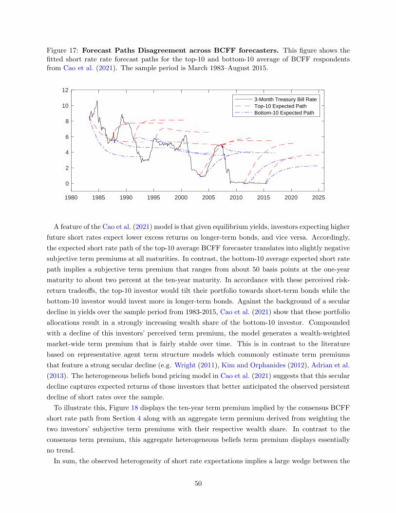
Figure 17: Forecast Paths Disagreement across BCFF forecasters. This figure shows thefitted short rate rate forecast paths for the top-10 and bottom-10 average of BCFF respondentsfrom Cao et al. (2021). The sample period is March 1983–August 2015.
1980 1985 1990 1995 2000 2005 2010 2015 2020 2025
0
2
4
6
8
10
12
3-Month Treasury Bill RateTop-10 Expected PathBottom-10 Expected Path
A feature of the Cao et al. (2021) model is that given equilibrium yields, investors expecting higher
future short rates expect lower excess returns on longer-term bonds, and vice versa. Accordingly,
the expected short rate path of the top-10 average BCFF forecaster translates into slightly negative
subjective term premiums at all maturities. In contrast, the bottom-10 average expected short rate
path implies a subjective term premium that ranges from about 50 basis points at the one-year
maturity to about two percent at the ten-year maturity. In accordance with these perceived risk-
return tradeoffs, the top-10 investor would tilt their portfolio towards short-term bonds while the
bottom-10 investor would invest more in longer-term bonds. Against the background of a secular
decline in yields over the sample period from 1983-2015, Cao et al. (2021) show that these portfolio
allocations result in a strongly increasing wealth share of the bottom-10 investor. Compounded
with a decline of this investors’ perceived term premium, the model generates a wealth-weighted
market-wide term premium that is fairly stable over time. This is in contrast to the literature
based on representative agent term structure models which commonly estimate term premiums
that feature a strong secular decline (e.g. Wright (2011), Kim and Orphanides (2012), Adrian et al.
(2013). The heterogeneous beliefs bond pricing model in Cao et al. (2021) suggests that this secular
decline captures expected returns of those investors that better anticipated the observed persistent
decline of short rates over the sample.
To illustrate this, Figure 18 displays the ten-year term premium implied by the consensus BCFF
short rate path from Section 4 along with an aggregate term premium derived from weighting the
two investors’ subjective term premiums with their respective wealth share. In contrast to the
consensus term premium, this aggregate heterogeneous beliefs term premium displays essentially
no trend.
In sum, the observed heterogeneity of short rate expectations implies a large wedge between the
50
beliefs of the marginal and the average investor. The findings thus show that the term structure of
disagreement about policy rate expectations is highly informative about the pricing of risk in the
bond market.
Figure 18: Aggregate term premiums. The figure compares the consensus term premium (redline) from Section 4 to the aggregate term premium obtained as the wealth-weighted average ofthe term premiums perceived by the top-10 and bottom-10 investors (black line) from Cao et al.(2021).
1982 1987 1993 1998 2004 2009 2015
-1
0
1
2
3
4
5
Wealth-weighted Ten-year Term PremiumConsensus Ten-year Term Premium
Disagreement and term premiums: other work. A growing recent literature has linked
forecast disagreement and the bond market. As already mentioned above, Wright (2011) shows
that the secular decline of term premiums implied by a standard affine model and model-free term
premiums implied by consensus survey expectations across ten developed economies coincide with
a decline of inflation forecast dispersion since the 1990s. Ehling et al. (2018) document empirically
that the dispersion of inflation expectations has a strong effect on real and nominal bond yields over
and above the impact of expected inflation. Buraschi and Whelan (2016) study the interactions
between risk aversion and disagreement and present a model where heterogeneous beliefs arise
because agents have different views about the (constant) long-run growth rate of consumption and
because their perceptions of the correlation of shocks differs. More recently, Buraschi et al. (2021)
aggregate individual expected excess bond returns based on forecasters past accuracy in predicting
interest rates. In line with the findings presented here, they document that disagreement about
bond risk premiums is time-varying and persistent. Barillas and Nimark (2019) build a structural
model of the term structure in which investors with heterogeneous information sets form higher-
order expectations about the beliefs of all other investors. Equilibrium bond prices then reflect a
speculative component which depends on investors beliefs about the error that the average investor
makes when predicting future short rates. Their model suggests that the speculative component
explains a sizable fraction of the variation in U.S. Treasury yields. Barillas and Nimark (2017)
generalize this model to allow for richer price of risk specifications as used in the empirical term
structure literature. In their model, investors observe heterogeneous signals of the state variables
driving bond yields. Finally, Giacoletti et al. (2021) build a dynamic term structure model in which
a representative investor updates her beliefs about future bond yields. They find that when this
51
updating is conditioned on the dispersion in bond yield forecasts, the model produces substantially
smaller forecast errors.
6 The Term Structure of Expectations in Structural Models
The analysis of the term structure expectations has yet to take a stand on the rationality of expec-
tations. We now develop a dynamic structural general equilibrium model in which the subjective
beliefs of households and firms are consistent with our reduced-form forecasting model. The struc-
tural model has the equilibrium property that subjective beliefs are more persistent than the true
data generating process. Household and firm expectations exhibit extrapolation bias, consistent
with empirical and laboratory evidence. That subjective and objective forecasting models differ
represents a departure from full-information rational expectations.
An advantage of a structural model is that we can estimate how different economic shocks deter-
mine forecast errors and the term structure of expectations. In principle, this permits addressing
some earlier questions—such as the determinants of real neutral rates and interest rate terms
premia—left unanswered by the reduced-form model. Having a structural theory of long-term
expectations permits analysis of important practical policy questions, that rational expectations
can not. For example, we argue that our framework provides a coherent definition of expectations
anchoring, and clear predictions of the economic conditions in which expectations will be anchored
or un-anchored. We show this has important implications for monetary and fiscal policy.
6.1 A General Structural Model
Dynamic stochastic general equilibrium (DSGE) models describe the behavior of economic agents
solving infinite-horizon intertemporal decision problems in a market economy. The equilibrium
behavior of the economy therefore depends primarily on the expected path of aggregate variables
such as prices, aggregate quantities and policy variables. The log-linear solution of a typical DSGE
can then be generally expressed as
A0zt =n∑s=1
An
(Et
∞∑T=t
λT−ts zT+1
)+An+1zt−1 +An+2εt
where the vector zt collects all models variables in deviation from their steady-state values; the
vector εt collects exogenous innovations; λs ∈ 1, ..., n are discount factors resulting from the agents’s
decisions rules; Ai for i ∈ 1, ..., n+ 2 coefficient matrices; and
Et =
∫ 1
0Eitdi
52
average beliefs. The representation holds for arbitrary beliefs, including rational expectations.27
Under this latter assumption the model has the equilibrium solution
zt = Φzt−1 + Φεεt.
Agents are fully informed about the economy steady-state; they face no information frictions leading
to fluctuating long-run beliefs. The matrix Φ measures the transitional dynamics around the steady
state, and Φε captures the economy’s impact response to innovations.
Now introduce an information friction to this full information benchmark. Consistent with our
simple model in sections 2.1 and 3.1 agents are uncertain about the long-run. Expectations are
then formed using the forecasting model
zt = ωt + Φzt−1 + νt (6.1)
ωt = ωt−1 + ηt (6.2)
where both the drift ωt and the innovations νt are unobserved to agents.28 Reflecting the perceived
slow-moving drift we further assume agents’ priors imply E [ηtη′t] = κ2
ω×E [νtν′t] where 1 >> κω > 0.
This signal extraction problem delivers the now familiar Kalman filter updating
ωt+1 = ωt + κω (zt − ωt − Φzt−1) (6.3)
= ωt + κω(zt − zt|t−1
)(6.4)
where zt − zt|t−1 denotes the short-term forecast error. Given the estimate ωt, forecasts at any
horizon T > t are determined as
EtzT = ΦT−tzt +T−t∑j=0
Φjωt (6.5)
while their estimate of the time-varying mean is
limT→∞
EtzT = (I − Φ)−1ωt. (6.6)
Evaluating expectations in the structural equations and combining with the belief updating
equation gives the true data generating process
zt = Γ× ωt + Φzt−1 + Φεεt
ωt+1 = [I + κω (Γ− I)] ωt + κωΦεεt
zt − zt|t−1 = (Γ− I)ωt + Φεεt
27All variables are expressed in log-deviations from their non-stochastic steady-state values. See Eusepi et al. (2020)for a detailed example and derivations. For an analysis of real business cycle theory see Eusepi and Preston (2011).
28For simplicity we assume the matrix Φ which governs short-run dynamics is known to agents.
53
where Γ is composite of structural parameters. Provided ωt is stationary, the rational expectations
equilibrium represents a limiting case of this model with κω → 0.29
Comparison with the reduced-form model of earlier sections reveals four new properties of struc-
tural models. First, forecast errors are determined by long-run drifts and model innovations. This
permits giving a structural interpretation to the economic determinants of the term structure of
expectations. Second, because economic decisions depend on the estimated drifts, dynamics exhibit
self-referentiality. Beliefs affect realized data, and the data in turn affect beliefs. The matrix Γ
determines the extent to which equilibrium outcomes depend on beliefs.30 Third, and related, the
model displays extrapolation bias (Fuster et al. (2010), Bordalo et al. (2020)) as an equilibrium
property.31 Subjective beliefs have a unit root, while the true data-generating process implies
beliefs evolve as an auto-regressive process of order one, with eigenvalues determined by
I + κω (Γ− I) .
The wedge between subjective and objective beliefs provides a metric of the importance of the
information friction from belief formation. And again, the use of a structural model permits
understanding how structural shocks and economic policy affect this wedge. Fourth, short-term
forecast errors as are not i.i.d., a further manifestation of bounded rationality.
We now consider two applications of this general framework. In both applications these general
properties are vital to being able to answer policy-relevant questions as well as providing a coherent
account of the data.
6.2 Application 1: Anchored Inflation Expectation
An important practical concern for policymakers is whether long-term inflation expectations are
well anchored or not. Greater stability of long-term inflation expectations improves the short-
run trade-off between inflation and output, improving welfare. Carvalho et al. (2021) propose a
structural model of inflation and inflation expectations which determines the economic conditions
under which long-term expectations will be well anchored. The model permits answering questions
like: what determines trend inflation? Will chronic undershooting of inflation targets lead to
downward drift and unanchoring of long-term inflation expectations? How can we reconcile large
negative output gaps and stable inflation during the Great Recession with positive output gaps and
high inflation during the Great Inflation?
The model comprises a new Keynesian aggregate supply curve
πt = µt + Et
∞∑T=t
(ξβ)T−t [κxT + (1− ξ)βπT+1] (6.7)
29That is the eigenvalues of I + κω (Γ− I) are inside the unit circle.30In the case that Γ = I the model would have a self-confirming equilibrium (see Sargent 1999). In general ‖Γ‖ < 1
so that beliefs are only partially self-fulfilling. This implies beliefs in equilibrium are stationary variables31Recall the discussion in section 3.4
54

where πt is inflation, xt the output gap, µt an exogenous i.i.d. cost-push shock. The parameters
0 < β, ξ < 1 are the household discount factor and the probability that the firm cannot re-optimize
their price in any given period. These parameters determine the slope of the aggregate supply curve
as κ ≡ (1− ξβ) (1− ξ) /ξ > 0. The central bank is assumed to control aggregate demand directly,
implementing monetary policy using the targeting rule
πt − π∗ + λxt = ϕrnt
where π∗ denotes the inflation target, the long-run mean of inflation, normalized to zero; λx the
stabilizing weight given to output gap stabilization; and ϕ > 0 potential deviations from optimal
policy.32 With the exception of the inflation target π∗, the policy rule is known and understood by
agents so that when combined with the aggregate supply curve, inflation is the only endogenous
variable to be forecast to make pricing decisions. The model is closed with a forecasting model that
has the same structure as above, though permits the Kalman gain to vary over time, as discussed
further below.
Evaluating expectations and some simple algebra gives the state-space representation
πt = Γπωπt + Φrnt−1 + Φεεt
ωπt+1 = [1 + κω,t (Γπ − 1)] ωπt + κω,t
where κω,t is a time-varying gain and the coefficient
0 < Γπ =1
1 + κλ−1x
(1− ξ)β1− ξβ
< 1
measures the degree of self-referentiality of expectations. Firms raise their optimal price when they
believe long-run inflation has risen, raising aggregate inflation. In turn, higher inflation leads firms
to markup their long-term inflation expectations. This interaction engenders an exogenous inflation
trend, determined by monetary policy and shocks to the natural rate of interest and markups.
Monetary policy regulates the strength of this connection. When λx → 0 the target criterion
is equivalent to strict inflation targeting, eliminating self-referential inflation dynamics. When
λx → ∞ the target criterion is equivalent to output gap targeting, and, for standard parameter
values implies values of Γπ near unity. Beliefs are near self-confirming.
How do firm’s form an estimate of the inflation target? Following Marcet and Nicolin (2003),
firms are unsure about the correct model to forecast inflation. They choose between two estimators
of the long-run mean of the inflation rate: either a decreasing gain algorithm, κω,t = κω,t−1 + 1; or
a constant gain algorithm, κω,t = κω. The first estimator is ordinary least squares. The gain is the
inverse of the sample size, so that accumulating evidence of a stationary mean leads to declining
32With ϕ = 0 and in absence of markup shocks the central bank implements optimal discretion where both outputgap and inflation are at their zero objective in every period while the nominal interest rate moves one-to-one withthe natural rate of interest. See Woodford (2003b).
55
sensitivity of long-run expectations to new information. The second estimator implies a constant
and relatively high sensitivity to new information. In the spirit of CUSUM tests, firms test the
hypothesis of a constant mean every period using a criterion based on cumulative forecast errors.33
Together these assumptions imply long-term inflation expectations display time-varying sensitiv-
ity to short-run forecast errors. This permits a formal definition of anchored expectations which
is directly tied to beliefs about inflation. Expectations are said to be anchored when beliefs are
consistent with the policy regime in place: a fixed inflation target. This occurs when firms do not
reject the hypothesis of a time-invariant inflation mean. Long-term inflation expectations display
decreasing sensitivity to forecast errors and, if they remain anchored, converge to the inflation tar-
get. However, large and persistent forecast errors can lead firms to abandon the belief of a constant
mean. Long-run beliefs are then unanchored and tightly connected to short-term forecast errors.
Figure 19 describes the model’s predictions for long-term inflation expectations for the U.S. and
three other countries. Parameters are estimated using nonlinear Bayesian methods on inflation
U.S. data, including survey-based professional short-term forecasts. However, measures of long-
term forecasts were not used in the estimation. The top panels shows how the model does a
remarkable job at predicting 5-10 year ahead expectations for all countries.34 For most of the
sample, the survey-based forecasts are inside the 95% credible set. The bottom panels display the
evolution of the learning gain. For all countries the sensitivity of long-term inflation expectations
to short-term forecast errors has changed over time and, in particular, signaled episodes of poor
anchoring. In the U.S. the 1970s marked over twenty years of volatile expectations, followed by firm
anchoring starting at the end of the 1990s throughout the financial crisis. Conversely, Japan has
consistently displayed poorly anchored expectations since the mid-1990s and Spain experienced
a brief episode of un-anchoring during the financial crises. Finally, Swedish long-term inflation
expectations become anchored following its adoption of inflation targeting in 1992.
Summing up, we have provided further evidence of a link between short-term forecast errors and
revisions in long-term expectations. Perhaps even more important, the structural model highlights
the structural breaks in the expectations formation process and how they capture the evolution of
measured long-term expectations in different countries.
6.3 Application 2: The Term Structure of Expectations
In practice, central banks use short-term interest rates to influence aggregate demand. To model the
transmission of monetary policy we supplement the aggregate supply equation with the aggregate
demand equation
xt = Et
∞∑T=t
βT−t [(1− β)xT+1 − (iT − πT+1 − rnT )] (6.8)
33Carvalho et al. (2021) provides details. This approach to model selections builds on Marcet and Nicolini (2003),Milani (2014) and Cho and Kasa (2015).
34Model’s predictions are made using the same parameters. The mean of inflation is, however, estimated separatelyfor each country.
56
where it is the one-period nominal interest rate, the instrument of monetary policy. The entire
future sequence of anticipated short rates matters for aggregate demand. Drfiting long-run interest
rate expectations represents an information friction that helps explain macroeconomic data and is
a challenge for stabilization policy.
For simplicity assume the central bank adopts the simple rule
it = φπt (6.9)
where φ > 1 is a policy parameter. Combined with the aggregate supply equation (6.7) and the
aggregate demand equation (6.8) the model has a rational expectations equilibrium of the form
zt = Φrnt−1 + Φεεnt
where zt = (πt, xt, it)′ and εnt the innovation to the natural rate of interest. Assume that under
imperfect information beliefs are given by (6.1) and (6.2) with ωt =(ωπ, ωx, ωi
), S an indentity
matrix, and lagged state vector replaced by the natural rate of interest. Long-term interest rate
forecasts are revised in response to short-term forecast errors according to
ωit+1 = ωit + κωi(it − ωit − Φir
nt−1
)(6.10)
= ωit + κωi(it − it|t−1
). (6.11)
where Φi is the element of Φ corresponding to the rational expectations solution for the interest rate.
Shocks to the natural rate of interest induce interest rate surprises leading to shifts in long-term
beliefs—indeed, the whole term structure of expectations.
Extrapolation bias is a equilibrium property of the model driving a wedge between subjective
and objective beliefs. To illustrate in the case of interest rates, consider an economy where prices
are nearly flexible, that is ξ → 0, and monetary policy is understood to be implement using the
simple rule. Taking the difference between agent interest-rate forecasts, Et, and model-consistent
projections under true data-generating process, Et, gives the wedge in any future period T > t
EtiT − EtiT =
(1− φ−1 − β
1− β
)ωit
= κωi ×(
1− φ−1 − β1− β
) ∞∑j=0
(1− κωi
1− φ−1
1− β
)jεnt−1−j (6.12)
where the second equality follows from writing current interest rate beliefs as a function of the entire
past history of natural rate innovations. Both the size of the learning gain and monetary policy
regulate the degree of extrapolation bias. Depending on the expectations formation mechanism
and monetary policy, transitory natural-rate shocks may have long-lived effects. For example, a
sequence of positive shocks to the natural rate leads to an increase in the wedge, leading to a
steeper path of the interest rate compared to that path which would be expected under the true
57

data-generating process. This wedge has empirical and policy implications.
Eusepi et al. (2020) estimate a medium-sized DSGE model using U.S. macroeconomic data, in-
cluding the term structure of interest rate and inflation expectations from professional forecasters.
The wedge between subjective and objective beliefs is vital to understanding and fitting the evolu-
tion of macroeconomic data as well as the Federal Reserves’ ability to pursue active stabilization
policy.35 For example, Figure 20 shows the fit of five-to-ten (black line) and one-to-ten (blue line)
expectations for both inflation and nominal short-term interest rate from a blend of Blue Chip
surveys (red and blue dot respectively). The DSGE model fits well the behavior of expectations
since the mid-1980s, while at the same time fitting shorter-term survey forecasts.36
The bottom panel plots agents’ subjective one-to-ten-year-ahead expectation for the short-term
nominal rate (black line) together with the model consistent expectation (blue line) held by an out-
side observer knowing the true data-generating process. Because of extrapolation bias subjective
expectations display weaker mean reversion and higher volatility compared to objective expecta-
tions. This wedge has economic content. Model consistent expectations would correctly predict
short-term rates to fall more quickly from the peak of the Great Inflation over the subsequent
Great Moderation period: a lower expected path of the short-term rate in turn would deliver lower
equilibrium long-term interest rates. Conversely, at the beginning of the sample, loose monetary
policy flattens the term structure of interest rate and forecasters systematically under-predicted the
significantly higher interest rates observed over the 1980s. It is also clear the the wedge between
subjective and objective expectations varies over time: over the last decade of the sample this
wedge shrinks significantly as long-term expectations stabilize. Finally, the figure also illustrates
that ten-year Treasury yields (red line) move together with subjective expectations, but still leave
a significant residual, as discussed in Section 4.2.
35See Giannoni and Woodford (2004).36See Eusepi et al. (2020) for further details. The estimation allows a structural break in the learning gain at the
end of the 1990s.
58
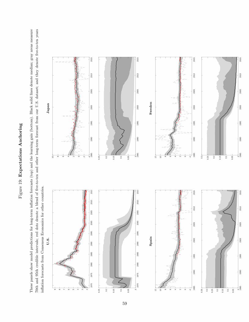
Fig
ure
19:
Exp
ecta
tion
sA
nch
ori
ng
Thes
epanel
ssh
owm
odel
pre
dic
tions
for
long-t
erm
inflati
on
fore
cast
s(t
op)
and
the
learn
ing
gain
(bott
om
).B
lack
solid
lines
den
ote
med
ian;
gra
yare
as
mea
sure
70th
and
95th
cred
ible
inte
rvals
;re
ddots
den
ote
able
nd
of
five-
to-t
enand
oth
erlo
ng-t
erm
fore
cast
from
our
U.S
.data
set;
and
they
den
ote
five-
to-t
enyea
rs
inflati
on
fore
cast
sfr
om
Conse
nsu
sE
conom
ics
for
oth
erco
untr
ies.
U.S
.Japan
1970
1975
1980
1985
1990
1995
2000
2005
2010
2015
23456789
1985
1990
1995
2000
2005
2010
2015
-4-202468
10
1970
1975
1980
1985
1990
1995
2000
2005
2010
2015
0
0.050.
1
0.150.
2
0.25
1985
1990
1995
2000
2005
2010
2015
0
0.050.
1
0.150.
2
0.25
Spain
Sweden
1985
1990
1995
2000
2005
2010
2015
-202468
1012
1985
1990
1995
2000
2005
2010
2015
-202468
1012
1985
1990
1995
2000
2005
2010
2015
0
0.050.
1
0.150.
2
0.250.
3
0.35
1985
1990
1995
2000
2005
2010
2015
0
0.050.
1
0.150.
2
0.250.
3
59
6.4 Implications for Monetary and Fiscal policy
The previous examples adduce further evidence that long-term movements in expectations inflation
and interest rate expectations are tied to short-term forecast errors and that this relationship is
time-varying. Eusepi et al. (2020) show that these properties of long-term expectations have impli-
cations for monetary policy. In contrast to a full-information rational expectations model, a central
bank cannot fully stabilize the macro-economy, even in the case of demand shocks. The degree
to which stabilization policy is compromised depends on how well anchored are long-term expec-
tations. As long-term expectations become less stable, aggressive aggregate demand management
becomes infeasible: large movements in overnight policy rates translate into volatility in long rates
and therefore aggregate demand. However, when long-term expectations are well anchored, model
predictions are much closer to those of a rational expectations analysis. The constraint posed by
the term structure of interest rate expectations is quantitatively important.
That activist stabilization policy is undesirable, contrasts with earlier papers by papers by Ferrero
(2007), Orphanides and Williams (2007) and Molnar and Santoro (2013). These papers emphasize
how non-rational expectations can alter the short-run trade-off in the new Keynesian Phillips curve
and conclude that optimal policy should be more aggressive than a rational expectations analysis.
However, this literature makes the assumption that the central bank can directly control aggregate
demand. Accounting for the transmission mechanism of monetary policy turns this result on its
head, because aggressive adjustment of overnight rates creates volatility in the term structure of
interest rate expectations.
Building on Eusepi et al. (2020), Eusepi et al. (2021) explore the implications for optimal mon-
etary policy at the zero lower bound. Their model addresses the common practical concern that
long-term inflation expectations might become un-anchored and drift downwards in response to
a large negative demand shock. They show unanchored expectations complicate monetary policy
requiring an extended period of zero interest policy because expectations themselves, if sufficiently
pessimistic, can cause the zero lower bound to be a constraint on policy actions. The optimal
forward guidance policy is front-loaded and displays an insurance principle: aggressive responses to
a negative demand shock are required to support inflation expectations in the case of a persistent
deterioration in economic conditions. However, policy is too stimulatory in the case of transi-
tory disturbances. These policy implications are strikingly different to Eggertsson and Woodford’s
(2003) rational expectations analysis.
Introducing fiscal and debt management policy further complicates inflation control in this class
of model. Eusepi and Preston (2012) and Eusepi and Preston (2018) show that when households
are uncertain about their long-run tax obligations, modeled in the same way as uncertainty about
long-run inflation or interest rates, then Ricardian equivalence fails to hold, even when the fiscal
authority has access to lump-sum taxation. Movements in expectations about taxes, inflation and
interest rates generate shifting valuations of the public debt and the expected tax burden attached
to that debt. The resulting wealth effects on aggregate demand complicates stabilization policy,
fundamentally changing the economy’s response to different kinds of disturbances. These effects
60
are larger for higher levels of average debt and for moderate debt maturities, and quantitatively
important for debt levels observed for the United States and other countries since the Great Re-
cession. These results raise obvious concerns about inflation policy over the coming decade, given
the substantial debt-financed stimulus packages in response to the global pandemic.
7 Conclusions and Further Directions
This chapter has provided a simple expectations formation mechanism to study and measure of
the term structure of expectations. Observed survey-based measures of expectations are consistent
with forecasters frequently revising their long-term outlook. In particular, these revisions are
partly associated to their short-term forecast errors, as predicted by standard statistical models
of trend and cycle decomposition. This holds for individual forecasts as well as for our measure
of the consensus term structure of expectations. In addition to fitting consensus expectations, the
proposed model provides valuable insights in the sources of forecast dispersion from short to long
horizons.
In the final section, we consider the implications of this expectations formation mechanism in
DSGE models. Here additional information frictions are imposed. In particular, economic agents
are boundedly rational and do not know the correct data generating process: consistent with much
empirical evidence, they tend to over-extrapolate from recent developments. Having estimated the
models using the term structure of expectations, we show that the proposed expectations formation
mechanism has profound implications for monetary and fiscal policy design when compared with
the benchmark of rational expectations.
The work explored also suggests interesting future avenues of investigation. First, both reduced-
form and structural model should allow time-varying components to the expectations formation
process. As shown in the last section, agents’ model validation process can lead to state-dependent
sensitivity of revisions of long-term expectations to short-term forecast errors. But time- and
state-dependence of information frictions can be more general. For example, the agents’ ability or
willingness to process information likely depends on the associated costs and benefits which may
change with the state of the economy.
Second, while models of information frictions with dispersed information are now ubiquitous
in macroeconomics, these models mostly focus on forecast dispersion over the short-term. In
contrast, our analysis suggests that disagreement about the long term is a key feature of survey
data. Incorporating learning about the long run in structural models of dispersed information could
deliver important implications for both business cycle analysis and monetary policy design.
Third, our measure of consensus expectations suggests that the term structure of interest rates
is driven only partly by the term structure of policy rate expectations. An overwhelming majority
of monetary models used for policy analysis instead assumes that the only transmission channel
of monetary policy is via short rate expectations. The results in this chapter help better quantify
the importance of this channel but also highlight the importance of additional channels, including
61

variation in term premiums, forecast dispersion or failure of equilibrium asset pricing restrictions
grounded on the assumption of perfect information and rational expectations.
Finally, while the reduced-form framework we have introduced offers a fairly flexible specification
that is able to provide a tight fit to the observed survey data, when incorporating the expectations
formation mechanism in a DSGE setup we made specific assumptions about information frictions.
While the literature has made remarkable progress in using survey data to select among competing
theories of expectations formation, the jury is still out. The measure of the term structure of
expectations that this chapter provides can be used to make further gains in selecting the models
that best describe the data, for example by studying the dynamic response of the term structure
of expectations to specific macroeconomic shocks.
62
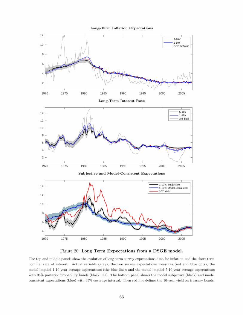
Long-Term Inflation Expectations
1970 1975 1980 1985 1990 1995 2000 2005
2
4
6
8
10
125-10Y1-10YGDP deflator
Long-Term Interest Rate
1970 1975 1980 1985 1990 1995 2000 2005
2
4
6
8
10
12
14 5-10Y1-10Y3M-Tbill
Subjective and Model-Consistent Expectations
1970 1975 1980 1985 1990 1995 2000 2005
4
6
8
10
12
141-10Y: Subjective1-10Y: Model-Consistent10Y Yield
Figure 20: Long Term Expectations from a DSGE model.
The top and middle panels show the evolution of long-term survey expectations data for inflation and the short-term
nominal rate of interest. Actual variable (grey), the two survey expectations measures (red and blue dots), the
model implied 1-10 year average expectations (the blue line); and the model implied 5-10 year average expectations
with 95% posterior probability bands (black line). The bottom panel shows the model subjective (black) and model
consistent expectations (blue) with 95% coverage interval. Then red line defines the 10-year yield on treasury bonds.
63
References
Adam, K., Matveev, D., Nagel, S., 2021. Do survey expectations of stock returns reflect riskadjustments? Journal of Monetary Economics 117, 723–740.
Adrian, T., Crump, R. K., Moench, E., 2013. Pricing the term structure with linear regressions.Journal of Financial Economics 110, 110–138.
Andrade, P., Crump, R. K., Eusepi, S., Moench, E., 2016. Fundamental disagreement. Journal ofMonetary Economics 83, 106–128.
Andrade, P., Le Bihan, H., 2013. Inattentive professional forecasters. Journal of Monetary Eco-nomics 60, 967–82.
Angeletos, G.-M., Huo, Z., Sastry, K. A., 2020. Imperfect macroeconomic expectations: Evidenceand theory. In: NBER Macroeconomics Annual 2020 , National Bureau of Economic Research,vol. 35, pp. 1–86.
Aruoba, S. B., 2020. Term structures of inflation expectations and real interest rates. Journal ofBusiness and Economic Statistics 38.
Bansal, R., Yaron, A., 2004. Risks for the long run: A potential resolution of asset pricing puzzles.Journal of Finance 59, 1481–1509.
Barillas, F., Nimark, K., 2019. Speculation and the bond market: An empirical no-arbitrage frame-work. Management Science 65, 4179–4203.
Barillas, F., Nimark, K. P., 2017. Speculation and the term structure of interest rates. Review ofFinancial Studies 30, 4003–4037.
Bauer, M. D., Rudebusch, G. D., 2020. Interest rates under falling stars. American EconomicReview 110, 1316–54.
Beechey, M. J., Johannsen, B. K., Levin, A. T., 2011. Are long-run inflation expectations an-chored more firmly in the euro area than in the united states? American Economic Journal:Macroeconomics 3, 104–29.
Bems, R., Caselli, F., Grigoli, F., Gruss, B., 2021. Expectations’ anchoring and inflation persistence.Journal of International Economics 132.
Bhamra, H. S., Uppal, R., 2014. Asset prices with heterogeneity in preferences and beliefs. Reviewof Financial Studies 27, 519–580.
Bianchi, F., Ilut, C., 2017. Monetary/fiscal policy mix and agents’ beliefs. Review of EconomicDynamics 26, 113–139.
Boero, G., Smith, J., Wallis, K. F., 2008. Uncertainty and disagreement in economic prediction:The bank of england survey of external forecasters. Economic Journal 118, 1107–1127.
Bordalo, P., Gennaioli, N., Ma, Y., Shleifer, A., 2020. Overreaction in macroeconomic expectations.American Economic Review 110, 2748–2782.
64

Buraschi, A., Piatti, I., Whelan, P., 2021. Subjective bond returns and belief aggregation. Workingpaper, Saıd Business School.
Buraschi, A., Whelan, P., 2016. Speculation, hedging, and interest rates. Working paper, ImperialCollege London.
Campbell, J. Y., Shiller, R. J., 1991. Yield spreads and interest rate movements: A bird’s eye view.Review of Economic Studies 58, 495–514.
Cao, S., Crump, R. K., Eusepi, S., Moench, E., 2021. Fundamental disagreement about monetarypolicy and the term structure of interest rates. Staff Report 934, Federal Reserve Bank of NewYork.
Carvalho, C., Eusepi, S., Moench, E., Preston, B., 2021. Anchored inflation expectations. AmericanEconomic Journal: Macroeconomics Forthcoming.
Chan, J., Clark, T., Koop, G., 2018. A new model of inflation, trend inflation, and long-run inflationexpectations. Journal of Money, Credit and Banking 50, 5–53.
Cieslak, A., 2018. Short-rate expectations and unexpected returns in Treasury bonds. Review ofFinancial Studies 931, 3265–3308.
Cochrane, J., Piazzesi, M., 2005. Bond risk premia. American Economic Review 95, 138–160.
Cochrane, J., Piazzesi, M., 2008. Decomposing the yield curve, working paper.
Cochrane, J. H., 2017. Macro-finance. Review of Finance 21, 945–985.
Cogley, T., Primiceri, G. E., Sargent, T. J., 2010. Inflation-gap persistence in the US. AmericanEconomic Journal: Macroeconomics 2, 43–69.
Cogley, T., Sargent, T. J., 2005. Drift and volatilities: Monetary policies and outcomes in the postWWII U.S. Review of Economic Dynamics 8, 262–302.
Coibion, O., Gorodnichenko, Y., 2012. What can survey forecasts tell us about informational rigidi-ties? Journal of Political Economy 120, 116–159.
Crump, R. K., Eusepi, S., Lucca, D., Moench, E., 2014. Which growth rate? It’s a weighty subject.Liberty Street Economics Blog.
Crump, R. K., Eusepi, S., Moench, E., 2011. A look at the accuracy of policy expectations. LibertyStreet Economics Blog.
Crump, R. K., Eusepi, S., Moench, E., 2018. The term structure of expectations and bond yields.Staff Report 775, Federal Reserve Bank of New York.
Del Negro, M., Giannone, D., Giannoni, M. P., Tambalotti, A., 2018. Safety, liquidity, and thenatural rate of interest. Brookings Papers on Economic Activity 49, 235–94.
Dovern, J., Fritsche, U., Slacalek, J., 2012. Disagreement among forecasters in G7 countries. Reviewof Economics and Statistics 94, 1081–1096.
Edge, R. M., Laubach, T., Williams, J. C., 2007. Learning and shifts in long-run productivitygrowth. Journal of Monetary Economics 54, 2421–2438.
65
Ehling, P., Gallmeyer, M., Heyerdahl-Larsen, C., Illeditsch, P., 2018. Disagreement about inflationand the yield curve. Journal of Financial Economics 127, 459–484.
Erceg, C. J., Levin, A. T., 2003. Imperfect credibility and inflation persistence. Journal of MonetaryEconomics 50, 915–944.
Eusepi, S., Giannoni, M., Preston, B., 2020. On the limits of monetary policy, working paper.
Eusepi, S., Gibbs, C., Preston, B., 2021. Forward guidance with unanchored expectations, workingpaper.
Eusepi, S., Preston, B., 2011. Expectations, learning and business cycle fluctuations. AmericanEconomic Review 101, 2844–2872.
Eusepi, S., Preston, B., 2012. Debt, policy uncertainty and expectations stabilization. Journal ofthe European Economics Association 10, 860–886.
Eusepi, S., Preston, B., 2018. Fiscal Foundations of Inflation: Imperfect Knowledge. AmericanEconomic Review 108, 2551–2589.
Evans, G. W., Honkapohja, S., 2021. Learning and expectations in macroeconomics. PrincetonUniversity Press, Princeton, NJ.
Fama, E. F., Bliss, R. R., 1987. The information in long-maturity forward rates. American EconomicReview 4, 680–692.
Ferrero, G., 2007. Monetary policy, learning and the speed of convergence. Journal of EconomicDynamics and Control 39, 3006–3041.
Fuster, A., Laibson, D., Mendel, B., 2010. Natural expectations and macroeconomic fluctuations.Journal of Economic Perspectives 24, 67–84.
Garbade, K., 1996. Fixed Income Analytics. MIT Press, Cambridge.
Garnier, C., Mertens, E., Nelson, E., 2015. Trend inflation in advanced economies. InternationalJournal of Central Banking 11, 65–136.
Giacoletti, M., Laursen, K. T., Singleton, K. J., 2021. Learning from disagreement in the U.S.Treasury bond market. Journal of Finance 76, 395–441.
Giannoni, M., Woodford, M., 2004. Optimal Inflation-Targeting Rules. In: The Inflation-TargetingDebate, National Bureau of Economic Research, NBER Chapters.
Grishchenko, O., Mouabbi, S., Renne, J.-P., 2019. Measuring inflation anchoring and uncertainty:A U.S. and Euro area comparison. Journal of Money, Credit and Banking 51, 1053–1096.
Gurkaynak, R., Levin, A., Swanson, E., 2010. Does inflation targeting anchor long-run inflationexpectations? Evidence from the U.S., UK, and Sweden. Journal of the European EconomicAssociation 8, 1208–1242.
Gurkaynak, R., Sack, B., Swanson, E. T., 2005. The sensitivity of long-term interest rates to eco-nomic news: Evidence and implications for macroeconomic models. American Economic Review95, 425–436.
66

Gurkaynak, R. S., Sack, B., Wright, J. H., 2007. The U.S. Treasury yield curve: 1961 to the present.Journal of Monetary Economics 54, 2291–2304.
Hamilton, J. D., 1994. Time Series Analysis. Princeton University Press, Princeton, NJ.
Holston, K., Laubach, T., Williams, J. C., 2017. Measuring the natural rate of interest: Interna-tional trends and determinants. Journal of International Economics 108, S59–S75.
Johannsen, B. K., Mertens, E., 2016. A time series model of interest rates with the effective lowerbound. Journal of Money, Credit and Banking Forthcoming.
Jouini, E., Napp, C., 2007. Consensus consumer and intertemporal asset pricing with heterogeneousbeliefs. Review of Economic Studies 74, 1149–1174.
Kim, D. H., Orphanides, A., 2012. Term structure estimation with survey data on interest rateforecasts. Journal of Financial and Quantitative Analysis 47, 241–272.
Kim, D. H., Wright, J. H., 2005. An arbitrage-free three-factor term structure model and therecent behavior of long-term yields and distant-horizon forward rates. Finance and EconomicsDiscussion Series 2005-33, Federal Reserve Board.
Kozicki, S., Tinsley, P. A., 2001. Shifting endpoints in the term structure of interest rates. Journalof Monetary Economics 47, 613–652.
Kozicki, S., Tinsley, P. A., 2012. Effective use of survey information in estimating the evolution ofexpected inflation. Journal of Money, Credit and Banking 44, 145–169.
Krishnamurthy, A., Vissing-Jorgensen, A., 2012. The aggregate demand for Treasury debt. Journalof Political Economy 120, 233–267.
Kydland, F. E., Prescott, E. C., 1982. Time to build and aggregate fluctuations. Econometrica 50,1345–70.
Lahiri, K., Sheng, X., 2008. Evolution of forecast disagreement in a Bayesian learning model.Journal of Econometrics 144, 325–240.
Laubach, T., Williams, J. C., 2003. Measuring the natural rate of interest. Review of Economicsand Statistics 85, 1063–1070.
Lucas, Robert E., J., 2003. Macroeconomic priorities. American Economic Review 93, 1–14.
Mackowiak, B., Wiederholt, M., 2009. Optimal sticky prices under rational inattention. AmericanEconomic Review 99, 769–803.
Mankiw, N. G., Reis, R., 2002. Sticky information versus sticky prices: A proposal to replace thenew keynesian phillips curve. Quarterly Journal of Economics 117, 1295–1328.
Mankiw, N. G., Reis, R., Wolfers, J., 2003. Disagreement about inflation expectations. In: NBERMacroeconomics Annual 2003 , National Bureau of Economic Research, vol. 18, pp. 209–270.
Marcet, A., Sargent, T. J., 1989. Convergence of least squares learning mechanisms in self-referentiallinear stochastic models. Journal of Economic Theory 48, 337–368.
Mertens, E., Nason, J., 2020. Inflation and professional forecast dynamics: An evaluation of stick-iness, persistence, and volatility. Quantitative Economics 11, 1485–1520.
67
Molnar, K., Santoro, S., 2013. Optimal monetary policy when agents are learning. European Eco-nomic Review 66, 39–62.
Orphanides, A., Williams, J. C., 2007. Robust monetary policy with imperfect knowledge. Journalof Monetary Economics 54, 1406–1435.
Patton, A. J., Timmermann, A., 2010. Why do forecasters disagree? Lessons from the term struc-ture of cross-sectional dispersion. Journal of Monetary Economics 57, 803–820.
Piazzesi, M., Salomao, J., Schneider, M., 2015. Trend and cycle in bond premia, working paper.
Primiceri, G. E., 2005. Time varying structural vector autoregressions and monetary policy. Reviewof Economic Studies 72, 821–852.
Rich, R., Tracy, J., 2010. The relationships between expected inflation, disagreement and uncer-tainty: Evidence from matched point and density forecasts. Review of Economics and Statistics92, 200–207.
Scheinkman, J. A., Litterman, R., 1991. Common factors affecting bond returns. Journal of FixedIncome 1, 54–61.
Sims, C. A., 2003. Implications of rational inattention. Journal of Monetary Economics 50, 665–690.
Stock, J. H., Watson, M. W., 1989. New indexes of coincident and leading economic indicators.In: NBER Macroeconomics Annual 1989 , National Bureau of Economic Research, vol. 4, pp.351–409.
Stock, J. H., Watson, M. W., 2007. Why has U.S. inflation become harder to forecast? Journal ofMoney, Credit and Banking 39, 3–33.
Summers, L. H., 2014. Reflections on the ‘new secular stagnation hypothesis’. Secular stagnation:Facts, causes and cures pp. 27–38.
Tambalotti, A., 2003. Inflation, productivity and monetary policy: From the great stagflation tothe new economy, working paper.
Timmermann, A. G., 1993. How learning in financial markets generates excess volatility and pre-dictability in stock prices. Quarterly Journal of Economics 108, 1135–1145.
Woodford, M., 2003a. Imperfect common knowledge and the effects of monetary policy. In: Aghion,P., Frydman, R., Stiglitz, J., Woodford, M. (eds.), Knowledge, Information and Expectations inModern Macroeconomics: In Honor of Edmund S. Phelps, Princeton University Press, pp. 25–58.
Woodford, M., 2003b. Interest and Prices: Foundations of a Theory of Monetary Policy. PrincetonUniversity Press.
Wright, J. H., 2011. Term premia and inflation uncertainty: Empirical evidence from an interna-tional panel dataset. American Economic Review 101, 1514–34.
Xiong, W., Yan, H., 2010. Heterogeneous expectations and bond markets. Review of FinancialStudies 23, 1433–1466.
Zarnowitz, V., Lambros, L. A., 1987. Consensus and uncertainty in economic prediction. Journalof Political Economy 95, 591–621.
68
Appendix A Defining Term Premiums
The term premium for an n period bond can be obtained from observed yields and expectationsvia the following identity:
yt(n) =1
nEt [it + it+1 + · · ·+ it+n−1] + tpt(n), (A.1)
where yt(n) is the continuously compounded yield on an n-month discount bond, it is the risk-freenominal short rate at time t, and tpt(n) is the nominal term premium. The term premium is thussimply given by the difference between observed yields and what would be the yield predicted bythe (pure) expectations hypothesis, i.e. the average expected future short rate over the life of thebond. It is important to emphasize that this is simply an identity; there are no implicit assumptionsabout the rationality or bias of expectations or the data generating process for yields, expectations,or term premiums.
In order to separate longer-term from short-term expectations, we conduct our analyses in termsof forward rates, defined as the current yield of an n-month bond maturing in n+m months:
ft(n,m) =1
n[(n+m)yt(n+m)−myt(m)]
Since the model is estimated at a monthly frequency, we construct annual forward rates as theannual average of monthly forward rates. We then define forward term premiums as the differencebetween ft(n,m) and the consensus expected short-term rate over the n months m months hence(i.e., a forward version of equation (A.1)):
tpfwdt (n,m) = ft(n,m)− 1
n
n+m∑i=m+1
Et [it+i]
For example, at our monthly sampling frequency the 9Y1Y forward term premium, i.e., the termpremium embedded in a one-year bond, nine years in the future, would be defined as:
tpfwdt (12, 108) = ft(12, 108)− 1
12
120∑i=109
Et [it+i]
A convenient way to gain intuition about forward rates versus yields is to consider the case whereterm premiums are zero at all maturities. Then 1-period forward rates, {ft(1, i) : i = 1, . . .} wouldbe given by Et [it], Et [it+1], Et [it+1] , . . ., whereas yields, {yt(n) : n = 1, . . .} would be
Et [it] ,1
2(Et [it] + Et [it+1]) ,
1
3(Et [it] + Et [it+1] + Et [it+3]) , . . .
In other words, once adjusted for term premiums, forwards reflect the expectation of the short rateat a specific horizon in the future whereas yields reflect the average expected short rate up to thathorizon. Accordingly, the term premium on a bond with n months to maturity simply reflects theaverage one-month forward term premium from 1 through n :
tpt(n) =1
n
n∑i=1
tpfwdt (1, i).
69
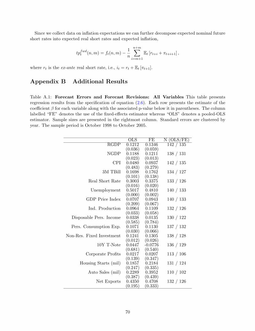
Since we collect data on inflation expectations we can further decompose expected nominal futureshort rates into expected real short rates and expected inflation,
tpfwdt (n,m) = ft(n,m)− 1
n
n+m∑i=m+1
Et [rt+i + πt+i+1] ,
where rt is the ex-ante real short rate, i.e., it = rt + Et [πt+1].
Appendix B Additional Results
Table A.1: Forecast Errors and Forecast Revisions: All Variables This table presentsregression results from the specification of equation (2.6). Each row presents the estimate of thecoefficient β for each variable along with the associated p-value below it in parentheses. The columnlabelled “FE” denotes the use of the fixed-effects estimator whereas “OLS” denotes a pooled-OLSestimator. Sample sizes are presented in the rightmost column. Standard errors are clustered byyear. The sample period is October 1998 to October 2005.
OLS FE N (OLS/FE)RGDP 0.1212 0.1346 142 / 135
(0.036) (0.059)NGDP 0.1188 0.1211 138 / 131
(0.023) (0.013)CPI 0.0480 0.0937 142 / 135
(0.483) (0.279)3M TBill 0.1698 0.1762 134 / 127
(0.101) (0.138)Real Short Rate 0.3003 0.3375 133 / 126
(0.016) (0.020)Unemployment 0.5017 0.4810 140 / 133
(0.000) (0.002)GDP Price Index 0.0707 0.0943 140 / 133
(0.209) (0.067)Ind. Production 0.0964 0.1109 132 / 126
(0.033) (0.058)Disposable Pers. Income 0.0338 0.0135 130 / 122
(0.585) (0.784)Pers. Consumption Exp. 0.1071 0.1130 137 / 132
(0.030) (0.066)Non-Res. Fixed Investment 0.1241 0.1305 138 / 128
(0.012) (0.026)10Y T-Note 0.0447 -0.0776 136 / 129
(0.681) (0.540)Corporate Profits 0.0217 0.0207 113 / 106
(0.139) (0.347)Housing Starts (mil) 0.1857 0.2184 131 / 124
(0.247) (0.335)Auto Sales (mil) 0.2289 0.3952 110 / 102
(0.387) (0.439)Net Exports 0.4350 0.4708 132 / 126
(0.195) (0.333)
70
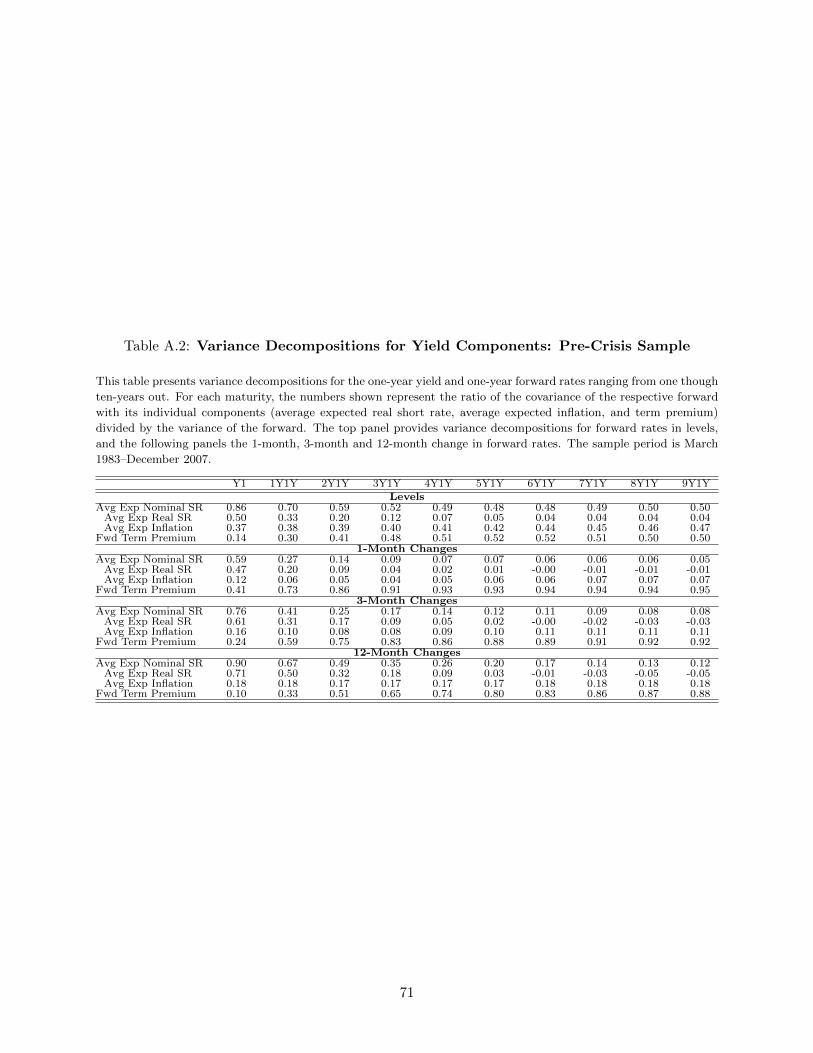
Table A.2: Variance Decompositions for Yield Components: Pre-Crisis Sample
This table presents variance decompositions for the one-year yield and one-year forward rates ranging from one though
ten-years out. For each maturity, the numbers shown represent the ratio of the covariance of the respective forward
with its individual components (average expected real short rate, average expected inflation, and term premium)
divided by the variance of the forward. The top panel provides variance decompositions for forward rates in levels,
and the following panels the 1-month, 3-month and 12-month change in forward rates. The sample period is March
1983–December 2007.
Y1 1Y1Y 2Y1Y 3Y1Y 4Y1Y 5Y1Y 6Y1Y 7Y1Y 8Y1Y 9Y1Y
LevelsAvg Exp Nominal SR 0.86 0.70 0.59 0.52 0.49 0.48 0.48 0.49 0.50 0.50
Avg Exp Real SR 0.50 0.33 0.20 0.12 0.07 0.05 0.04 0.04 0.04 0.04Avg Exp Inflation 0.37 0.38 0.39 0.40 0.41 0.42 0.44 0.45 0.46 0.47
Fwd Term Premium 0.14 0.30 0.41 0.48 0.51 0.52 0.52 0.51 0.50 0.501-Month Changes
Avg Exp Nominal SR 0.59 0.27 0.14 0.09 0.07 0.07 0.06 0.06 0.06 0.05Avg Exp Real SR 0.47 0.20 0.09 0.04 0.02 0.01 -0.00 -0.01 -0.01 -0.01Avg Exp Inflation 0.12 0.06 0.05 0.04 0.05 0.06 0.06 0.07 0.07 0.07
Fwd Term Premium 0.41 0.73 0.86 0.91 0.93 0.93 0.94 0.94 0.94 0.953-Month Changes
Avg Exp Nominal SR 0.76 0.41 0.25 0.17 0.14 0.12 0.11 0.09 0.08 0.08Avg Exp Real SR 0.61 0.31 0.17 0.09 0.05 0.02 -0.00 -0.02 -0.03 -0.03Avg Exp Inflation 0.16 0.10 0.08 0.08 0.09 0.10 0.11 0.11 0.11 0.11
Fwd Term Premium 0.24 0.59 0.75 0.83 0.86 0.88 0.89 0.91 0.92 0.9212-Month Changes
Avg Exp Nominal SR 0.90 0.67 0.49 0.35 0.26 0.20 0.17 0.14 0.13 0.12Avg Exp Real SR 0.71 0.50 0.32 0.18 0.09 0.03 -0.01 -0.03 -0.05 -0.05Avg Exp Inflation 0.18 0.18 0.17 0.17 0.17 0.17 0.18 0.18 0.18 0.18
Fwd Term Premium 0.10 0.33 0.51 0.65 0.74 0.80 0.83 0.86 0.87 0.88
71