the term structure of securities lending...

The Term Structure of

Securities Lending Fees

FRANÇOIS COCQUEMAS*

This version: November 1, 2017

ABSTRACT

Stock lending is typically an overnight agreement where short sellers pay a fee for borrowinga security. The lending is subject to rerating and recall risk, which may prevent them fromholding their position open until it pays off. An alternative is to construct a synthetic shortposition using options. The two markets are linked by arbitrage. I jointly estimate the termstructure of implied securities lending fees and implied volatility from options data. I find thatthe implied lending fees co-vary with the spot fee. They include a premium indicative of large,low-probability jump risk. Implied lending fees and implied volatility are positively related;however, the estimated term structure of implied volatility is on average flat across horizons.This suggests the volatility term structure may be less useful to model than the lending fee termstructure. Finally, I find a median lending fee risk premium of 2% per annum. It is much higherfor hard-to-borrow stocks and shorter maturities. Close to two-thirds of the risk premium canbe predicted using the term structure of implied lending fees.

Please find the latest version at this link:

https://www.cocquemas.com/files/de2b/JMP.pdf

JEL classification: G12, G13, G14

Keywords: option pricing, securities lending, short selling, term structure

*Vanderbilt University, Owen Graduate School of Management. [email protected]. I thankBob Whaley for his guidance, and I am grateful for conversations and comments from Peter Haslag, Sebastian Infante,Abraham Lioui, Miguel Palacios, Tom Smith, and Hans Stoll. This research was supported by the Vanderbilt FinancialMarkets Research Center, and computations were conducted in part using a grant from Amazon Web Services.

1

https://www.cocquemas.com/files/de2b/JMP.pdf

mailto:[email protected]

The ability to sell assets short underpins much of financial theory. Given the prohibition of

“naked” short selling, it depends on the existence of a securities lending market. Without it, short

sellers could not borrow shares to sell, and could not set up their position. It would be much harder

for asset prices to adjust and reflect available information. Liquidity would also be dramatically

impacted. It may thus be surprising that the securities lending market is opaque and full of frictions.

Indeed, this market is over-the-counter and tiered. Borrowers do not get access to the same pool

of assets. They do not pay the same fees for the same assets. No market rate is available1.

Securities lending is compensated by a lending fee. It is a stochastic process linked to loan

supply (“shortability,” per D’Avolio, 2002), hardness-to-borrow (“specialness,” ibid.), and recall

risk. Through these three channels, short selling strategies are risky: the position may have to be

closed before it pays off (see for instance Engelberg, Reed, and Ringgenberg, forthcoming). The

stock may become prohibitively expensive to borrow, or be recalled. At the same time, the supply

might dry up, and opening a new short would become impossible.

As Duffie, Gârleanu, and Pedersen (2002) point out, “lending fees reflect the expectation of

future shorting demand.” For most borrowers, the lending fee can typically be adjusted daily by

the lender, according to supply and demand. When option market makers delta-hedge by selling in

the spot market, they incur this borrowing cost. They are exposed to changes in the fee over the

life of the options. Therefore, they need to take that cost into account when setting their spreads.

This paper argues that lending fees should enter, together with payouts, into the net cost of carry

that affect option valuation. This is easy to see for European options, which can be used to construct

a synthetic short position through put-call parity. Conversely, if one observes option prices, then

it should be possible to extract implied lending rates at different maturities, corresponding to an

expected average fee that is locked in over the time horizon. This implied fee needs to incorporate

jump risk in the spot lending fee.

In this paper, I estimate the term structure of implied lending fees and show that it is consistent

with a lending jump risk premium. Option markets imply that lending fees have a small probability

of jumping high, with a somewhat rapid reversal. This is reflected in a downward sloping term

structure. Indeed, a large jump would have time to revert for longer-dated options, and be averaged

out. For shorter maturities, it may not.1Due to the opaqueness of the market, it is hard to estimate formally how much of these differences stem from

counterparty risk. Anecdotal evidence suggests that it is not the only factor. The lack of automation in many segmentsof the market prevents larger agent banks from engaging in transactions with a broader client base, above and beyondcounterparty risk.

2

This matches realized dynamics of the spot lending fee. The magnitude of the implied is higher,

however, in line with a tail risk premium. I jointly estimate the term structure of volatility and find

that, unconditionally, it is on average flat across horizons. This suggests that, to explain observed

option prices at different horizons, it might be preferable to model stochastic lending fees over

stochastic volatility (or to model both).

The securities lending transaction has parallels to an overnight repurchase agreement: the lend-

ing rate can change from day to day (rerating of the loan), and the lender can initiate a recall

forcing the return of the security by T+3 (or T+6 for market makers)2. This can turn into a prob-

lem if lending fees and recalls spike right as the short position is about to pay off, compromising

the ability to profit from the bet. On the other hand, options allow participants to lock in a certain

lending rate to maturity as part of their quotes. That rate should therefore embed a premium for

the market maker’s assessment of the lending fee risk.

Indeed, even the easiest-to-borrow stocks (general collateral, or G.C. stocks henceforth) face a

“peso problem.” However infrequently, G.C. stocks become “special,” most often as a response to

negative events and increased short interest. The jump can be drastic. It can take lending fees from

the lower to the top decile from one day to the next. Option market makers who write synthetic

shorts would gain a long exposure. They can hedge by short selling the security3. Under Regulation

SHO, they cannot engage in naked short selling. They would then have to pay the lending fee, which

can evolve over time until the options mature. They therefore need to consider that risk into their

bid-ask spread. Empirically, this has been shown to be the case during the 2008 short-sale ban on

financial stocks (Battalio and Schultz, 2011; Grundy, Lim, and Verwijmeren, 2012). Market makers,

unable to hedge, dramatically adjusted their quotes to discourage investors from creating synthetic

shorts.

Given most single-name equity options are American, put-call parity will be an inequality and

will not enable traders to construct a synthetic short as such. However, the lending rate should

still be reflected in the convenience yield of derivatives (after accounting for discrete dividends).

To back out the implied lending fee, I develop the following approach: for a given maturity, I take

a put-call pair with the same strike and jointly estimate the implied volatility and implied lending

fee that best match observed prices. I use the bid price for the call and the ask price of the put, as

well as the ask price for the spot. Using two options allows me to disentangle the implied volatility2Or, failing that, a buy-in.3This is in contrast with markets with liquid futures, such as index options.

3

and the lending rate.

I find that the estimated term structure of lending fees significantly co-moves with the spot rate,

supporting the methodology. The spot lending rate alone explains up to 34% of the term structure

rates, depending on the horizon. The implied rates are higher for the shorter maturities, and they

converge to the spot rate for longer-dated options. They are also higher than the realized average

rate for the period they cover. This is consistent with the existence of a risk premium. The median

lending fee risk premium is around 2%, but it can be significantly larger for stocks that are harder

to borrow and for shorter maturities.

This paper contributes to a growing literature on the functioning of the securities lending market

and its relevance to a number of anomalies. It is most closely related to Muravyev, Pearson, and

Pollet (2016), who extract a proxy for the spot lending rate from options. They do not find a lending

fee risk premium. This contrasts with my findings, likely due to differences in data and methodology.

It also relates to Kalay, Karakaş, and Pant (2014), who consider a similar methodology to try and

extract the value of corporate voting rights. I do not look specifically at voting, but it is one of the

components that should be compensated by the lending rate. The methodology I use differs from

both papers. They rely on an (inexact) put-call parity to obtain their measures, which I do not. I

focus on obtaining results at different horizons. I also jointly estimate a term structure of volatility.

Like these papers, however, I use at-the-money options to derive my estimates.

The securities lending market has been the subject of increasing industry and regulatory atten-

tion. Mutual funds and ETFs in particular are deriving ever greater revenues from their lending

activities (Blocher, Cocquemas, and Whaley, 2017), and realizing an increasingly large share of

their potential lending revenues. Some of these funds could afford to no longer charge management

fees, in exchange for a larger shares of lending revenues. In line with this rise in prominence, the

Securities and Exchange Commission recently introduced Form N-PORT. Funds will have to make

more detailed and more frequent disclosures on securities lending activities. So far, these trends did

not translate into a larger share of the stocks being available to be lent out overall. According to

Markit data, the value of available securities to market capitalization (“lending capacity,” or “loan

supply” in Engelberg et al., forthcoming) did not display a clear trend over the 2008-2016 sample

period (Table 1). Over that time, 20% to 30% of the easiest-to-borrow securities are available to

lend. Securities “on special” have more variability, but no clear temporal trend is apparent.

This paper is organized as follows. Section I outlines the methodology for extract lending fees

from option prices, and discusses the relevant literature and methodological concerns. Section II

4

details the data sources and the implementation of the methodology, and presents some summary

statistics. Section III examines the estimation results, confirms the pertinence of the methodology,

and infers some properties of the lending rate and volatility dynamics. Section IV analyses the

lending fee and volatility risk premia derived from the model. Section V concludes.

I. Extracting Lending Fees from Option Prices

A. The Term Structure of Implied Lending Fees

Derivatives pricing typically includes a cost of carry component, which takes into account the costs

and benefits of holding the underlying position instead of the derivative product. For stocks, the

dividend yield is factored in as the only source of income by most of the stock options literature.

However, lending shares out is also a potential way to obtain income from a long position in the spot

market, and should be included in the convenience yield (i.e. a negative cost of carry). Rather than

using a continuous dividend yield, it is usually preferable to model discrete dividends, especially

with close-to-the-money American options. Discrete dividends introduce jumps that may make

early exercise optimal when it may not be with a continuous dividend yield. Then, what is left in

the convenience yield is the potential revenue from lending out the security, or expected average

lending rate.

In this paper, I extract the implied convenience yield and implied volatility from an option

pricing model using discrete dividends, for every available maturity. This produces a joint term

structure of lending fees and volatility. In order to estimate these two parameters, I need to observe

the prices of two options. Selling a call and buying a put, which for European options would

correspond to a synthetic short, is one possibility, but any two at-the-money options should do, as

long as the bid price is used for calls, and the ask price for puts. I then find the implied volatility

and convenience yield that match the observed market prices the best.

This methodology would also capture a voting rights premium, as modeled in Kalay et al.

(2014). Arguably, that premium is part of the securities lending fee, since the recipient of the

security also obtains voting rights. I do not make any attempt to parcel out voting rights.

Closely related to this paper, Muravyev et al. (2016) extract implied lending fees from options

prices, although they are not constructing a term structure, but rather a proxy for the spot lending

fee. They rely on put-call parity, which does not assume any particular option pricing model; how-

ever, it does not hold exactly for American options, and they have to apply a statistical adjustment

5

to account for the early exercise bias. They also do not estimate implied volatility, given it does

not enter put-call parity4. Finally, they use midpoints, which can be quite different from the actual

quotes a synthetic shorter would have to pay. Given this setup, they find no evidence of a lending

fee risk premium, but do conclude that the predictability of returns based on option spreads and

skews disappears in favor of their lending fee proxy, suggesting hardness-to-borrow may be the

source of the predictability.

This also relates to the literature on the cost of carry/convenience yield for derivatives valua-

tion. While often considered exogenous in the pricing of derivatives, the large fluctuations in the

convenience yield across time for many assets suggest that it should be derived in equilibrium.

Jarrow (2010) proposes a useful characterization of these additional premia, over and beyond the

more obvious direct costs and benefits of storing a commodity, as two embedded options: a scarcity

option, which essentially corresponds to potential lending revenues, and a usage option, correspond-

ing to potential cash flows from using the commodity, for instance as an input to production. In

the case we are concerned with, stocks, only the scarcity option is relevant: ultimately, borrowing

securities is costly because their supply is limited (and stochastic).

The idea that the convenience yield is stochastic goes back to Geske (1978) introducing a

stochastic dividend yield into the framework of Black and Scholes (1973). However, the focus on

the cost of carry has been mostly in the commodities strand of the literature, where the concept has

a more direct meaning. For derivatives on equities, the main focus has been to model stochastic

volatility, notably as a way to better match the empirical distribution of stock prices (and its

departure from log-normality). For American options in particular, few papers have looked at a

stochastic convenience yield, and surprisingly, even fewer have recognized lending revenues as a

necessary component of the net cost of carry. Even typical G.C. rates of 25bps per annum are large

in a low interest rate context, and lending fees can sometimes jump one or two orders of magnitude.

Some recent papers have attempted to fill this gap. Avellaneda and Lipkin (2009) model the

buy-in risk for hard-to-borrow stocks as a Poisson process, which Ma and Zhu (2017) develop into

an American option pricing model. Jensen and Pedersen (2016) explicitly models “severe frictions”

including short-sale costs, funding costs, and spot transaction costs. They find that these frictions,

and the lending fee in particular, can explain a significant amount of early exercises, especially

for shorter maturities. Atmaz and Basak (2017) propose a pricing model for the bid and ask of4The implicit assumption is that a call and a put with the same strike have the same implied volatility. This is

an explicit assumption in my methodology.

6

European options under short-selling costs or ban. The lending rate enters the cost of carry, and

they include a parameter for partial lending. However, they do not model dynamics of the lending

fee or early exercise.

This paper does not develop or rely on a specific framework for pricing options with shorting

costs. Instead, within a standard American option pricing model, I consider the cost of carry to

be the risk-free rate minus the lending fee. Discrete dividends are accounted for separately. I allow

the fee (and the volatility, and the risk-free rate) to be different at each maturity, so that I can

construct a term structure. The lending fee represents an average expected fee that is locked into

the option price when it is purchased. Those forward implied fees can then be compared either to

the spot (overnight) lending rate, or to the realized rate over the life of the option.

B. The Term Structure of Implied Volatility

In the process of estimating a term structure of implied lending fees, I also estimate a term structure

of volatility (for at-the-money options). There is a large literature on estimating and analyzing the

term structure of implied volatility, and in fact the volatility surface, where strikes are another

dimension.

A considerable number of approaches has been proposed to model the dynamics of implied

volatility, mostly on European options, and often on index options (see for instance Stein, 1989;

Harvey and Whaley, 1991; Heynen, Kemna, and Vorst, 1994; Xu and Taylor, 1994; Cont and

da Fonseca, 2002; Cont, Fonseca, and Durrleman, 2002; Fengler, Härdle, and Villa, 2003; Fengler,

Härdle, and Mammen, 2007; Andersen, Fusari, and Todorov, 2015). However, few papers tackle

the cross-section of equity options. Christoffersen, Fournier, and Jacobs (2017) is an exception,

proposing a factor analysis of the term structure of equity options’ implied volatility (on 29 stocks),

developing a factor-model for valuing the options. Şerban, Lehoczky, and Seppi (2008) studies a

multivariate stochastic volatility model with systemic factors, and estimate it on a cross-section of

options on the index and 13 stocks. Empirically, Elkamhi and Ornthanalai (2010) find a 3% market

jump risk premium embedded in the cross-section of options on the 32 largest firms in the S&P

500.

The cross-section in this paper is much larger, with a total of 792 stocks. However, this means

that some estimates for some stock-dates are missing (usually because of missing options data),

which makes most of the analyses of these papers (such as principal component analysis) difficult

without modifications. I therefore mostly rely on panel regression techniques.

7

Next, I describe the data and the implementation of the estimation methodology.

II. Data and Implementation of Methodology

A. Data Sources

Options data comes from OptionMetrics. The sample covers January 1996 through April 2016, but

it is restricted to 2008 forward. This is to match the securities lending data, and also for regulatory

reasons. Option market makers were initially exempted from Regulation SHO, and profited from

strategic failure-to-delivers (Evans, Geczy, Musto, and Reed, 2009). Since 2008, this is no longer

the case, and market makers cannot engage in naked short selling. Because computational costs

are high, the analysis is focused on the stocks that have one of the 100 highest dollar open interests

across options on at least one day of the sample. This comes to a total of 792 stocks (identified by

their unique CRSP permno) in the panel.

Data on the spot market, in particular stock bid-ask spreads and distributions, comes from

CRSP (accessed through WRDS). It is matched to OptionMetrics using the multipronged script

proposed by WRDS, which uses fuzzy name matching when other identifiers have failed. Finally,

data on interest rates comes from the Federal Reserve Board website (H.15 Daily Release).

Securities lending data comes from Markit’s Buyside Premium Data Feed and starts in 2008.

There are two main variables for the indicative fees. The Daily Cost of Borrow Score (DCBS)

classifies the fee charged by agent lenders in ten bins, from 1 (cheapest to borrow) to 10 (most

expensive to borrow). On the other end, the SAF variable is the simple average of fees on borrow

transactions from hedge funds, and is a numerical variable. Note that hedge funds may not be

representative of the market as a whole; the tiered nature of the relationships could make the rates

diverge significantly. Furthermore, using a simple average rather than a (value-)weighted average

may introduce some biases in this context.

From Markit data, I use not only the SAF variable and the DCBS categories, but also a few

other variables. Utilization is the value of assets on loan over total lendable assets. I also construct

a variable for the percentage of market capitalization available to loan, which gives a relative size of

the pool to loan. These two measures proxy for shortability. Tenure is the weighted average number

of days for open transactions. I also look at the number of open loan transactions, concentration

of value on loan among lenders, concentration of value on loan among brokers as controls, which

proxy for both liquidity and divergence of opinions.

8

The main variable for lending fees, SAF, is missing for 12% of observations, whereas DCBS is

missing for 0.3%. I impute the missing SAF observations using several categories of predictors:

1. Securities lending: DCBS score, utilization, tenure (weighted average number of days for

open transactions), number of open loan transactions, concentration of value on loan among

lenders, concentration of value on loan among brokers;

2. Stock characteristics: stock permno (categorical), SIC industry code (categorical);

3. Daily market data: log market capitalization, daily trade volume to market capitalization

ratio;

4. Intraday spreads: quoted spread (time-weighted), effective spread (value-weighted, Lee-

Ready signed), price impact (value-weighted, Lee-Ready signed).

The intraday spread indicators are derived from NYSE TAQ data. Securities lending data is from

Markit. Other data is from CRSP. I do not include any volatility measure, as the imputed SAF

variable will be related to implied volatility in later statistical analyses.

Imputation is performed using the Multivariate Imputation via Chained Equations approach

(MICE, see van Buuren and Groothuis-Oudshoorn, 2011), which works iteratively to fill predictive

variables with missing data5.

B. Summary Statistics

Table I shows basic summary statistics for the combined data sets. Panel A reports the mean and

some quantiles of each measure. The spot lending fees, proxied by SAF, are unsurprisingly very low;

likewise, the DCBS score is greater than 1 only for one eighth of the sample (88% of the sample is

G.C.). Due to our sample selection procedure, market capitalization is fairly large among the 792

stocks, with a median of $9.3bn; the first percentile is only $236m. Shorting risk probably matters

particularly for small stocks; unfortunately, these do not typically have liquid options to perform

the analysis reliably. In spite of this, the sample includes observation across the whole spectrum of

hardness-to-borrow.

Average turnover ratio is 2%. Relative bid-ask spreads for the underlying asset are all sub-

penny, as we are dealing with very liquid stocks. The lending capacity (value available to loan to5The method uses the Predictive Mean Matching technique for numeric variables, a polytomous logistic regression

for categorical variables (stock identifier and industry) and a proportional odds model for the (ordered) DCBS score.The assumption is that the missing data is missing at random, which may or may not be the case.

9

market capitalization) is 23% on average. Utilization of that capacity is 18% on average. Those

two measures show large inter-quantile ranges. Next, Markit’s three measures of concentration are

used: inventory, loans outstanding, and broker demand, standing at 0.16, 0.28 and 0.24. A higher

measure means fewer lenders/brokers, and a measure of 1 would mean a single one. The average

tenure is the weighted length in days of open positions, which has a median of 50 days and a mean

of 65 days. Finally, the number of open loans reported to Markit is shown. The median is 173 and

the average is 331.

Panel B reports the correlation matrix between the measures. Only the lower triangular part

in shown. All correlation coefficients are significantly different from 0 at the 0.1% level. SAF and

DCBS have an 86% correlation (using for simplicity DCBS as a continuous variable), which may

not be as high as one would expect. Markit does not detail the construction of its DCBS score,

and the SAF measure is imperfect, being a simple average of hedge funds lending rates. SAF also

has a 0.5 correlation with utilization, and a -0.2 correlation with the lending capacity: more supply

translates into a lower rate, and vice versa. Inventory concentration is positively related to the

spot rate, and loan and broker demand concentrations negatively related to it, indicating potential

pricing power when concentration on either side gets high. Longer average tenure and a greater

number of open loans both correlate with a higher fee.

[Table I about here.]

Table II shows the transition matrix between specialness categories, as proxied by Markit’s Daily

Cost of Borrow Score. The values indicate the frequency (Panel A) or relative frequency (Panel

B) that a firm is in the row i on a certain day moves to column j on the next day. The absolute

frequencies are very skewed due to the vast majority (88%) of observations being G.C./DCBS 1.

However, there is a non-zero amount of jumps from G.C. to special, including straight from DCBS

1 to DCBS 10. This is consistent with the idea that there might be a risk of large, infrequent

jumps which has to be embedded in the term structure of lending fees as market makers price their

options.

Panel B clearly shows strong daily persistence of hardness-to-borrow. Almost 100% of G.C.

stocks remain in that category the following day. There is significantly more variation for stocks

on special, but they also tend to remain in the same specialness category (between 81% and 86%,

except for the highest DCBS, where it is up to 95%).

[Table II about here.]

10

Table III shows the serial autocorrelation of the spot lending fee, computed for lags 1 through

360, with only some select lags reported. As apparent in Panel A, daily autocorrelation is high

and persistent. The median autocorrelation is still at 11% after 90 lags, and 4% after 180 lags.

Panel B shows the daily partial autocorrelation, i.e. the autocorrelation controlling for all shorter

lags. The partial autocorrelation falls much faster, as could be expected; however, for the median

observation, it is still not zero after thirty lags. This confirms the high persistence in lending fees

for the sample, in line with the literature on short selling constraints (e.g. Asquith, Pathak, and

Ritter, 2005; Blocher and Zhang, 2017).

[Table III about here.]

Table IV shows the transitions between specialness categories conditional on a transition having

occurred in the previous period (from any DCBS to any other DCBS). Diagonal values are still

high: after one day, between 59% and 70% of stocks have jumped to a DCBS between 2 and 9

stay in that same category. For stocks having moved to DCBS 1 and 10, it is up to 79% and 76%

respectively. However, the effect slowly fades away after 10 and 20 trading days, as shown in Panel

B and C. Only stocks in DCBS 1 mostly resist this effect (still at 74% after 20 days), consistent

with the idea that for most stocks, G.C. is the long-term state they revert to. Looking off the

diagonal, it appears that for stocks not staying in the same category, more than half fall back to

a lower category, but a large minority instead climb to a higher category. There appears to be a

stronger reversion effect towards G.C., but it is balanced by some further upward jumps. The jump

process seems to be self-exciting, where previous jumps make further jumps more likely.

[Table IV about here.]

Table V looks at the persistence of specialness conditional on a jump from G.C. (DCBS 1) to

special (DCBS ≥ 2). Overall, stocks jumping from G.C. to special are back in G.C. after just one

day in 41% of case. More than two thirds are back in G.C. after ten trading days. There is therefore

a lot of quick reversals after a jump, but also a fair amount of persistence. After one day, the second

most likely outcome (or the most likely for DCBS 2, which is the bulk of jumps from DCBS) is

not a reversal, but a continuation in the same category, as visible on the diagonal. However, that

diagonal largely disappears after 10 periods, and almost completely after 20. It is worth noting

that there are few cases of stocks jumping directly from DCBS 1 to a DCBS greater than 4, as was

already apparent in Table II.

11

[Table V about here.]

The time series of the lending capacity, i.e. the share of market capitalization available to lend,

is shown in Figure 1. The measure is remarkably stable for G.C. stocks, except for a drop around

the end of 2008. It is more variable for stocks on special, but without displaying any clear trend.

Stocks with DCBS 4 and 5 appear to display the most variation day-to-day. For stocks in the 25th

percentile with a DCBS between 2 and 5, it appears that it is not infrequent for the ratio to fall to

zero, which would likely mean the supply of shares to loan disappears entirely.

[Figure 1 about here.]

C. Implementation of Methodology

For each day and security, I pick the options that are closest to the money, as they tend to be the

most liquid6. I find the convenience yield and volatility that minimize the sum of squared errors

between the observed option prices and their theoretical value. To compute theoretical prices for

the American options, I use a finite difference lattice following the Crank-Nicolson method, which

works well for discrete dividends (see for instance Achdou and Pironneau, 2005). I use the bid price

for the call and the ask price of the put, as well as the ask price for the spot7.

For distributions, I assume perfect foresight of regular dividends, and of special dividends only

if they have been announced prior to the estimation date. A vast amount of corporate finance

literature studies the persistence of regular dividends, seemingly because cutting them would send

a costly negative signal. I do not have a way to deal with the risk of dividends being cut, which

in some rare cases (if there is prior expectation of it happening) might be a problem. The case of

special dividends that would be announced after the current date is also quite difficult to handle,

as there might be some prior expectation of them built into prices. For lack of a way to tease them

out, they are assumed away8.

A few filters on the data are applied along the way. I drop securities that could not be match be-

tween OptionMetrics and Markit using CUSIP. I then eliminate option series where OptionMetrics6For robustness, I used several options within some moneyness bounds instead, over a subsample. The resulting

implied fees and volatilities were similar, but the computing time increases linearly with the number of option series,which was cost-prohibitive.

7In robustness checks (available upon request), I used the midpoint for both the options and the underlying stock;the implied lending fees still appear to track the observed spot lending fees quite well, but their magnitude is higher.

8The general monotonicity of the estimated term structures seems to confirm ex post that this is rarely an issue:otherwise we would observe a jump between maturities straddling the special dividend.

12

was not able to compute an implied volatility rate, which indicates some underlying data error. I

do not actually use their implied volatility variable outside of this filter, as I estimate it together

with the securities lending rate.

Computationally, this is an “embarrassingly parallel” optimization problem, but it does require

a significant amount of processing power.The differential evolution algorithm (Price, Storn, and

Lampinen, 2006) was used for optimization, as a good trade-off between speed and accuracy with

no dependence on initial values. The sum of squared errors is minimized, although another norm

would likely work just as well.

D. Methodological Questions

D.1. Spot Dynamics

How variable are lending rates? The vast majority of stocks are lent out at the G.C. rate, in

transactions that are in effect collateralized financing transactions (typically, lenders receive 104%

of the value of the stock in cash, in exchange for a rebate). However, even these stocks occasionally

become more expensive, sometimes significantly so.

Blocher and Zhang (2017) document persistence across time of securities lending fees, for both

G.C. and special stocks. Stocks tend to remain in the “expensiveness” category over sustained

periods of time. I perform a similar analysis, although on daily data rather than smoothed over a

month, using the Daily Cost of Borrow Score (DCBS) categories from Markit in Table II, detailed

in Section II. I also look at the autocorrelation of the spot lending fee in Table III. Very large day-

to-day jumps appear to be infrequent, but they do happen, much more frequently when a previous

jump already occurred, as shown in Table IV and Table V.

The dynamics of the lending fee seem to be affected by a few key variables. Blocher, Reed, and

Wesep (2013) find that changes in supply can matter for firms “on special” even when utilization

(i.e. the number of lent out securities relative to the supply) is on the low side. In a rare real-

life experiment, Kaplan, Moskowitz, and Sensoy (2013) manipulate the supply of lendable shares.

They observe a reaction on the lending fee and the quantity lent, but find no evidence of it affecting

returns, volatility, skewness or spreads.

All in all, the spot dynamics amply justify turning to the option markets to look into a possible

risk premium to compensate for a potential jump risk.

13

D.2. Utilization Ratio

Holding a long position in a security allows for potential revenue from lending it out. However,

there is rarely demand for 100% (or more) of a security to be lent out for short selling. Even if

lenders were picked at random (and they are not, since this is an over-the-counter, tiered market),

you could not expect to consistently lend out all of your portfolio and maximize lending revenue.

There is therefore an argument for adjusting the lending fee by some factor to take into account

actual demand for the stock. One such factor is utilization, i.e. the ratio of securities lent out to

those “available to lend” (which can be hard to determine). However, the spot lending rate is the

income rate of the security conditional on being lent out.

Jensen and Pedersen (2016) point out it is possible that “the lender earns less than the short-

seller pays since the difference is lost to intermediaries (custodians and brokers) and search costs

and delays.” I follow their argument. This is a major problem in available data on securities lending

costs anyway: the rates that are available are only an approximation of what any borrower would

pay, and are in no way a market-wide rate. The main source for lending rates in academic papers,

Markit, only provides an equal-weighted rate for hedge funds, and no longer provides disaggregated

positions to researchers. Data from individual brokers is not only difficult to obtain, it will also only

ever be fragmentary. Finally, for most lenders, there is simply no public data on which fraction of

their inventory they are successfully lending out (their private utilization ratio).

Given these limitations, and for simplicity of interpretation, I do not apply a utilization ratio

to the spot lending rate. It should be kept in mind that estimates of the realized lending income

will be biased upward because of this, and that as a consequence the risk premia could be larger

than estimated.

D.3. Liquidity

There are reasons to worry about option liquidity, particular at the two ends: towards expiration

and at the longest horizons. There is a wide literature on option-expiration anomalies (for early

examples, see e.g. Feinstein and Goetzmann, 1988; Herbst and Maberly, 1990; Stoll and Whaley,

1997). Some mispricing phenomena have been documented with options that are about to expire, at

least in part due to strategies being rolled over. Among the effects, abnormal trading and volatility

in the underlying are widely reported (e.g., Ni, Pearson, and Poteshman, 2005).

The lack of liquidity at certain maturities, particularly longer ones, is likely related to the

14

uncertainly about expected lending fees. Christoffersen, Goyenko, Jacobs, and Karoui (forthcoming)

find risk-adjusted return spreads of 2.5% to 3.4% per day for illiquid vs liquid at-the-money options,

consistent with equity options market makers holding risky net long positions. This is in line with

the idea developed earlier that market makers wanting to hedge would have to incur securities

lending costs, and need to factor in that risk into their prices. However, they use intraday effective

spreads, i.e. the distance between the trading price and the quotes midpoint, to proxy for option

illiquidity. In other words, if trades generally occur at one of the prevailing quotes, then the effective

spread would be very closely related to the quoted spread at trading times.

In other words, at least for at-the-money option, it is likely that the identified option illiquidity is

closely linked to the shorting risk in the spot: if the underlying stock becomes harder to borrow, the

quoted bid-ask spread (and thus the effective spread) should widen9. The results of Christoffersen

et al. (forthcoming) may therefore need to be viewed with that interpretation in mind. A more

traditional take on illiquidity could likely be observed from the hedged returns of options that are

further in-the-money or out-of-the-money, or perhaps from realized spreads and price impacts.

All in all, I do not specifically deal with illiquidity other than by applying the filters described

above. For the reason just mentioned, it is likely that there is a fair amount of conceptual (and

practical) overlap between shorting costs and traditional measures of illiquidity.

D.4. Recalls

In the absence of frictions or supply constraints in the securities lending market and the underlying

spot market, recall risk should not be priced. In effect, if the lender needs the shares back, she can

just borrow instead, even for a high fee, since she can pass it through by readjusting the fee for

her outstanding contract to match. Likewise, the borrower would be indifferent to a recall, since he

would be able to find another security at the same market rate. In equilibrium, then, there would

be no recalls, especially given the three-day (or five-day) delay on delivery.

Why, then, would a lender initiate a recall, rather than use the alternatives? There must be

another motive for this action. There is some evidence that active funds monitor the value of

their corporate votes and recall if they believe it more valuable than the lending income (Kalay

et al., 2014; Aggarwal, Saffi, and Sturgess, 2015). They could presumably borrow shares themselves

instead of recalling, where delivery would not be at T+3 (or T+6) like a recall; but it may have9One solution would be to compute a spread from option pairs instead, comparing the long and short synthetic

underlying, or an approximation thereof for American options.

15

become difficult to locate more shares as the supply is finite, especially for funds owning a large

share in a company. That would be the precise situation when the voting rights are most valuable

to the fund, but maybe not as much to dispersed holders of the lent out securities. Still, they could

raise the rate on their lent out securities to match their private value, which could drive some of

the beneficial owners to close out their positions.

Overall, the recall has to be the consequence of frictions in the securities lending market. The

rebate rate should adjust accordingly, but there are conceivably situations where the supply may

disappear, no matter the price. This is markedly more likely in a tiered, over-the-counter market

where not all participants are trading with each other. In this type of setting, it is also possible

that relationship considerations may come into play. For instance, the lender may close the position

of a particular borrower in order to favor another; this type of motives (and perhaps a few more

nefarious ones) may not be priced through the rebate rate, but instead correspond to non-financial

and/or longer-term reputation or repeated interaction benefits.

In light of this, it is not crucial to model recalls separately. They are akin to the lending fee

becoming infinite (for certain participants) as available supply disappears.

In the next section, I turn to the estimation result for the term structures of implied lending

fees and volatility.

III. Estimation Results

A. Estimated Term Structure of Implied Lending Fees

In this section, I analyze the results from the estimation. To make the maturities more comparable,

I interpolate between available maturities using linear splines. This does not seem like a problematic

assumption given the estimated term structures are almost always monotonic.

Table VI shows summary statistics for the implied lending fees extracted from the at-the-money

option quotes at various maturities. Overall, the median fee is 2.4%, with some large outliers

bringing the mean up to 10%. Panel A shows the implied lending fee by maturity. It appears that

across the board, the fees are getting closer to zero as the maturity increases. The median fee is

as high as 31% for options maturing within the week, which may reflect an expiration effect, or

accounting for the (small) risk of a (high) jump that would not have time to be smoothed out over

a longer period (or effectively trigger early exercises). The fact that the decreasing term structure

pattern is consistent would lend more credence to the latter, although they are not exclusive.

16

Panel B distinguishes lending fees by specialness instead. Unsurprisingly, the implied fees in-

crease with the specialness category (proxied by DCBS from Markit). The easiest-to-borrow stocks

have a median implied fee of 2%, while the hardest are as high as 61%.

There is a number of negative lending fees in lower percentiles. They are rare, and Panel B

shows they are also concentrated in the cheaper-to-borrow stocks (mostly G.C. and DCBS lower

than 3). There is no way to rule out issues with the data or microstructure frictions, but there is

another possible explanation. A lot of the securities lending activity at the G.C. rate is not in itself

very profitable for the lenders, especially after accounting for operational costs. One of the reason

to lend out cheap stocks, then, is as a financing operation to receive cash collateral (in the bond

market, see Foley-Fisher, Narajabad, and Verani, 2016; Huh and Infante, 2017). A lender could

accept a negative fee if they need cash for financing other operations.

Finally, Panel C crosses the maturity and specialness categories for the median fee. The previous

patterns still hold; the fees increase with specialness and decrease with maturity. Once again, it

appears that options expiring within the week have extremely high implied fees. Harder-to-borrow

stocks have the highest fees. This reveals an expectation that stocks already under shorting pressure

will continue to be, and are more likely to undergo further upward jumps in the lending rate.

[Table VI about here.]

Figure 2 shows the estimated implied lending fee over the spot lending fee (SAF from Markit),

computed as i0,t− i0, where i0 is the continuous spot rate and i0,t (t ≥ 1) is the implied continuous

rate estimated from options with maturity t. The term structure is generally decreasing, and above

the spot rate, although there are some exceptions. The most central estimates appear to converge

towards the spot rate as the maturity increases. There is a sometimes significant wedge between

the implied fee and the spot fee for shorter maturities.

The option prices lock in an average lending fee, so they have to account for the probability of

jumps. The observed shape of the term structure is therefore consistent with a small risk of large

jumps in the lending fee. The short rates are higher presumably because a jump would not have

time to be averaged out before the expiration of the option, but also because it is more likely to

make early exercise profitable (Jensen and Pedersen, 2016). The longer rates are lower because

even if there is a jump, it will be smoothed out over time, and early exercise is less likely to be

preferable to keeping the option open.


17

Figure 3 separates out different categories of specialness (as proxied by the DCBS). The pattern

is robust across the groups, also it does appear flatter and more dispersed as the stock becomes

harder to borrow. This flatter pattern reveals a higher expected persistence for stocks that are

harder to borrow, i.e., conditional on a jump in lending fee, the return to the initial fee will be

slower. The greater inter-quantile dispersion indicates that either the jump is expected to be bigger

for stocks already on special or, possibly, the arrival intensity of jumps is higher. We tease apart

these interpretations in the next section.


These visual observations are confirmed more formally using regressions. Table VII shows panel

regressions of the implied lending fees for the different maturities on the spot lending fee. In Panel

A, which does not include any control, we observe that the term structure overreacts to changes

in the spot rate (coefficient for SAF greater than 1), all the more that the maturity is close. This

reflects the decreasing shape of the term structure observed in Figures 2 and 3. For maturities

shorter than a week, the coefficient for SAF is 3.9, meaning that for a percentage point increase in

the spot rate, the short implied rate increases by almost 4 percentage points. The level of reaction

progressively goes down as the maturity increases, reaching 1.1 for maturities greater than a year.

Given no other controls, the explanatory power of the spot rate is non negligible, at least for

maturities greater than two weeks (R2 over 25%), but a large part of the variation is not explained

by it alone. Adding firm-fixed effects (Panel B) increases the adjusted R2 of the regressions to

around 45%, consistent with the idea that fees are persistent within stocks. It also lowers the

coefficient on the spot rate, but it is still close to 2 for the shorter horizons, and falls below 1 after

six months. Adding time-fixed effects increases the R2 to above 50% at almost all horizons, but

does not change the qualitative interpretation.

[Table VII about here.]

Figure 4 shows the time series of the implied lending fee and volatility over the estimation

sample. For each day and firm, the median of the rates at each horizon is taken. The plots shows

the twenty-fifth percentile, median and seventy-fifth percentile across firms for that day. It appears

that the implied lending rate has some spikes during the sample, particularly at the end of 2008, at

the end of 2013 and since the end of 2014. The patterns look consistent with mean reversion, and

possibly multiple regimes. Turning to the time series of implied volatility, some similar patterns

18

are observed, with spikes largely matching that of the implied lending rate, although they appear

proportionally less extreme, especially comparing the seventy-fifth percentiles.


Figure 5 and Figure 6 decompose these series according to the specialness category (DCBS).

For both the implied rate and the implied volatility, the median level is higher as the stocks are

harder to borrow, and there appears to be more volatility in the day-to-day patterns, with bigger,

more frequent spikes.



B. Estimated Term Structure of Implied Volatility

Next, we examine the estimated term structure of implied volatility, which was estimated jointly

with the term structure of implied lending fees.

Table VIII shows summary statistics for implied volatility. Overall, the median implied volatility

is 35% and the mean is 41%. Looking at maturities in Panel A, it appears that implied volatility is

very flat between 33% and 37% at the median (possibly with a slightly positive trend). The mean

is between 39% and 42% with no clear trend. Turning to hardness-to-borrow in Panel B, implied

volatility is increasing with specialness. The median observation for the easiest-to-borrow stocks

is 34%, which goes up to 89% for the hardest-to-borrow. Looking at inter-percentile ranges, there

is however a lot of overlap between each specialness category. Panel C reports the median implied

volatility across maturity and specialness categories. The previous patterns are confirmed. For each

DCBS, the median implied volatility is flat across horizons, and it increases as the DCBS increases.

[Table VIII about here.]

Figure 7 shows the general shape of the term structure. As before, to ease the averaging as

maturities slide from day to day, I interpolate between two maturities using linear splines. Except

for the very short maturities, the term structure appears to be flat. Remember that each maturity

is estimated separately, so there are not inherent constraints in the methodology that would force

volatilities across maturities to be so close to each other. Given that it has been estimated jointly

19

with the lending fee, this may indicate that, as far as option pricing is concerned, it might be more

important to model a stochastic implied fee rather than stochastic volatility.

It is not obvious why the shortest maturities (less than a week) are a little higher (or much

higher at the highest percentiles). It may be linked to pricing anomalies have been reported in the

option market right before expiration, as contracts are being rolled over into the next-to-expire

maturity.

On top of the stability of implied volatility across horizons, it is also interesting to look at levels.

For most of the days and firms, it appears that the implied volatility is significantly higher than

the trailing realized volatility.


Figure 8 decomposes the implied volatility by hardness-to-borrow (along the Daily Cost of Bor-

row Score from Markit). The pattern looks almost identical along specialness categories. However,

the levels of implied volatility get higher as the stocks become harder to borrow. This makes in-

tuitive sense: stocks that are hard-to-borrow tend to have significant short interest, and a higher

likelihood of a subsequent price decrease, which often translates into higher volatility. Option mar-

ket makers therefore incorporate a larger implied volatility for securities on special compared to

the trailing realized volatility.


Next, I analyze the joint term structure of lending fees and volatility.

C. Estimated Joint Term Structure of Lending Fees and Volatility

In the estimation phase, both the implied lending fee and implied volatility were estimated at the

various maturities.

Table IX shows the panel regressions of the implied lending rate over implied volatility. It

appears that the two measures are significantly and positively related. Changes in implied volatility

explain more around 25% of changes in the implied lending fee at the various maturities. The

coefficients decrease as the maturity increases, which is consistent with the idea that more volatile

stocks are more likely to become in high shorting demand. A higher implied volatility at a long

horizon seems to have less impact on the lending fee than at shorter ones.

20

Adding firm-fixed effects again increases the R2 to between 40% and 45%, except for the longest

maturities (35%). It also lowers the coefficients on the implied volatility. Combining time- and firm-

fixed effects lowers them even more for the shorter maturities, but increases them for the longer

ones, making them somewhat flatter. In all cases, there is still a significant effect of the implied

volatility on the jointly estimated lending fee. This stresses the importance of jointly modelling

these two variables.

[Table IX about here.]

Table X shows the panel regressions of the implied lending rate over the spot lending rate and

implied volatility. Compared to the previous tables, both variables are still significant and most of

the interpretations are still the same. The shortest implied lending rate becomes lower than the

second shortest, possibly indicating that implied volatility is a better predictors of implied lending

rate jump at that horizon. The R2 are higher but in line with previous tables.

Panel C introduces a number of controls instead of the time- and firm- fixed effects. The spot

lending fee (proxied by SAF) still has more impact at shorter maturities than longer ones, except

for the shortest (7 days or less). The effect of implied volatility also decreases as the maturity gets

longer. Trailing realized volatility is not significant for the shortest maturities (up to 15 days), but

comes in negatively beyond that. It thus appears that, controlling for implied volatility, a higher

level of past volatility results in a lower implied lending fee after two weeks, possibly because of

mean reversion in volatility (and it being correlated to lending fees). Surprisingly, after controlling

for the spot fee, utilization is negative and significant, although the magnitude is very small. A 1pp

increase in the utilization ratio translates into less than 0.2pp (down to 0.02pp) decrease in implied

fees. The higher the inventory concentration, the higher the implied fee, with a much larger impact

at shorter horizons10 The lender concentration for the value actually on loan comes in positive

and significant for the shortest maturity, but is not significant at any other horizon. Neither is the

concentration of broker demand. Finally, the larger the market capitalization, the lower the implied

fee, though again the effect appears to have a much larger magnitude the shorter the maturity11.

[Table X about here.]10Markit does not detail the concentration formulas, except to say it is related to the sum of squared market

shares and that smaller numbers indicate a large number of lenders/brokers, and 1 means a single one. That makesthe interpretation of the regression coefficients less precise.

11In the interest of space, regressions with only one control at a time are relegated to the Online Appendix.

21

[Table X (cont.) about here.]

Having discussed the estimated implied lending and volatility rates, I now turn to the analysis

of the risk premia by comparing the expected to realized values.

IV. Risk Premia

A. Lending Fee and Volatility Risk Premia

So far, we have looked at the term structure of implied lending fees and volatility as they relate

to contemporaneous or trailing spot counterparts, but not realized lending income and volatility.

In this section, I consider the risk premia implied by the forward estimates of the lending and

volatility rates.

The volatility risk premium (and the variance risk premium) have been the subject of a lot

of literature (see for instance Bollerslev, Gibson, and Zhou, 2011, and references therein). It is

typically defined as the difference between implied and realized volatility over a certain horizon.

Muravyev et al. (2016) propose to compute a lending income risk premium, using an analogous

definition, as the difference between the implied and realized lending income rates, defined as the

average spot lending rate (SAF from Markit) over the life of each option. I follow this definition

in this section. However, likely due to differences in methodology, I do reach a vastly different

conclusion.

Table XI shows some summary statistics for the lending fee and volatility risk premia across

horizons. Over all maturities, the estimated lending fee risk premium is 8.2% per annum on average,

with a median of 1.8%. The median lending fee risk premia are mostly decreasing with the horizon,

starting at 29% for the shortest maturities down to less than 3% for maturities greater than a

month. The mean is larger (reaching 56% annually for maturity less than a week), driven by some

large outliers.

The median implied volatility risk premia are extremely consistent across maturities, between

17.5% and 18.5%, and slightly higher at 20.2% for contracts expiring within the week. Means are

about 4-6pp higher across the board. The overall median is 18.4%, and the average 22.8%.

[Table XI about here.]

Table XII shows the same statistics, this time computed across all maturities but separated by

specialness (as proxied by Markit’s DCBS). Moving from G.C. (DCBS 1) to special, the median

22

lending fee risk premia increase from 1.8% to 18% per annum for DCBS 9 and even 31% for the

hardest-to-borrow category, DCBS 10. Again due to some large outliers, the mean lending fee risk

premia are much higher, reaching 54% for the hardest-to-borrow stocks.

Similarly, the volatility risk premia increase as stocks get harder to borrow. Just jumping from

G.C. to the cheapest category of specialness, the median volatility risk premium doubles from 17%

to 34% per annum, and climb to 72% for the hardest to borrow stocks.

[Table XII about here.]

Table XIII shows the median risk premia only, but cross-tabulated along maturity and special-

ness categories. Looking at the lending fee risk premia (Panel A), it is first noticeable how large

the premia are for the shortest maturity (less than seven days), across levels of specialness. This

can be explained several (non-exclusive) ways. First, the jump probability in the spot lending fee

is low, but conditional on the jump, the effect can be large. This is more likely to have an impact

at shorter maturities, in part because there is less time for the jump to revert and its effect to be

smoothed out, in part because it might affect the optimality of the early exercise of the American

options. The second possibility is there is mispricing for options close to expiry.

Turning to median volatility risk premia, they appear to be strikingly flat across maturities

within each specialness category, in line with previous results. The levels increase considerably

with hardness-to-borrow, going from 16-18% for G.C. stocks to 71-75% annually for the hardest-

to-borrow stocks. The maturity-week volatility premia do appear somewhat higher than other

maturities, but the gap is rather small.

[Table XIII about here.]

Table XIV shows the panel regressions of the realized lending income over the implied lending

fee at each maturity. Looking at Panel A (no controls), it appears that the implied lending rate

is strongly related to the realized rate. However, the realized rate is smaller in magnitude. For

instance, for options maturing in more than 31 and less than 60 days, a 1pp increase in the implied

lending fee corresponds to an 11bp increase in the realized rate. The coefficient tends to increase

with maturity (except for horizons longer than a year), which should be viewed in relation with

the decreasing lending fee term structure. Without controls, the implied lending fee explain up to

33% of changes in the realized rate, explaining the most for maturities between 31 days and a year.

23

Time-fixed effects (Panel C) do not increase the R2 much, but firm-fixed effects bring them to the

52%-64% range.

Note that these are not predictive regressions, since we use the term structure on day t to explain

the realized lending fee until maturity, including day t. However, especially for longer maturities, it

is unlikely that day t holds much weight. The predictive regressions using the lagged term structure

are shown in the next subsection.

[Table XIV about here.]

Table XV adds implied volatility as a predictor in the previous regressions at each maturity. It

appears to be positively and significantly related to the realized lending rate in almost all cases.

However, it does not not seem to increase the adjusted R2 much over and beyond the implied

lending fee. This is another argument to focus on modeling the implied lending fee dynamics when

concerned about the term structure of options12.

[Table XV about here.]

Table XVI adds the spot lending fee (SAF) to the regressions of Table XIV. Given the persistence

of the spot lending fee, documented earlier in this paper, it is unsurprisingly a very good predictor

of the realized rate13. For shorter maturities, the coefficient is close to 1, dropping as maturity

increases (still at 0.76 for maturities above a year). However, the implied lending fee is still positive

and significant in all cases, with or without fixed effects. Even without fixed effects, the R2 reaches

98% for the shorter maturities, and goes down to 90% for 31- to 60-day maturities and 66% for

maturities greater than a year.

[Table XVI about here.]

B. Risk Premia Dynamics Over Time

The dynamic of the lending fee risk premia over time, shown in Figure 9, largely seem to track those

of the implied lending fee. Given there are more maturities within a short horizon, this may partly

be a byproduct of picking the median value across the term structure, as they tend to be much12Explaining the cross-section of strikes, and the smirk/smile, probably requires including volatility dynamics,

too.13Note that, once again, the spot rate enters the calculation of the realized rate, to the proportion of one day out

of remaining days to maturity.

24

higher than the realized rates. The time series for the volatility risk premia are also interesting,

with the medium dipping into the negative in the second half of 2008 and again more briefly in the

second half of 2011.


Figure 10 and Figure 11 decompose the risk premia into specialness categories. The patterns

appear roughly similar, although it appears that the lending fee risk premia can often become

negative (particularly for the 25th percentile), especially as the stocks are harder to borrow.



Overall, these analyses point to the existence of an at-times large and time-varying lending fee

risk premium, which is greater for shorter maturities and for harder-to-borrow stocks. Next, I look

at whether the term structure can help predict the realized income.

C. Predicting Realized Lending Fees

In this subsection, I consider whether it is possible to predict the realized lending income between

the next day and each option’s maturity, from variables known today, mainly the spot and implied

lending fees.

In order to do this, I reproduce the panel regressions from the previous subsection, this time

using lagged predictors to ensure no look-ahead bias. Table XVII shows the regression of the realized

income rate over the lagged implied lending fee other lagged controls. Despite the lag, unsurprisingly

the results are largely unchanged. The imply lending fee is still a significant predictor of the realized

lending fee, even though the spot rate contributes much more predictive power due to persistence.

Implied volatility comes in significantly, but barely seems to increase the explanatory power of the

regression.

Looking at regressions with all controls in Panel E, it appears that the spot lending fee, the

implied volatility, utilization, and the log of the trailing 250-day variance of utilization are significant

at all horizons. The implied lending fees remain significant at all maturities except the shortest

(less than a week). The log of the trailing 250-day variance of spot fees (related to the shorting

risk of Engelberg et al., forthcoming) is only significant for two of the longer maturities. It does

25

not seem that adding all of these variables contributes much over and beyond the spot lending rate

alone.

Overall, it seems easy to predict a large share of the realized lending rate at the various points

of the term structure using just the spot rate, and other variables do not help much, including the

implied lending fees. This is a byproduct of the extremely high persistence of the spot lending fees.

[Table XVII about here.]

[Table XVII about here.]

D. Predicting Lending Fee Risk Premia

Finally, Table XVIII shows a similar analysis of the lending fee risk premia as predicted by lagged

variables such as implied and spot lending rates. The role of these two lagged variables is inverted

compared to the previous subsection. While both are positive and significant predictors of the risk

premia on their own at each maturity, the implied lending fee explains 55% to 69% (Panel A),

while the spot lending fee only explains 2% to 16% (Panel B). Combining both variables does not

increase the explanatory power much beyond the implied lending (Panel C), but interestingly, the

spot lending rate now has a negative coefficient. This makes sense since the risk premium is the

implied minus the realized spot rate; however, in Panel B, the spot rate served to capture the level

of the risk premium, which the implied lending rate does in Panel C (as well as D and E).

Turning to the regressions with all controls in Panel E, it is once again noticeable that the R2

are left largely unchanged. The implied and spot lending fees are consistently significant across

horizons, as is the log market capitalization. Implied volatility and average tenure are significant

for all maturities but one. Utilization is significant for maturities longer than 31 days, while the

log of the trailing 250-day variance of utilization is significant for maturities less than 90 days,

as is inventory concentration. The log of the trailing 250-day variance of spot fees (related to the

shorting risk of Engelberg et al., forthcoming) is again only significant for longer maturities, this

time above 61 days.

[Table XVIII about here.]

[Table XVIII (cont.) about here.]

26

While predicting the lending fee risk premia is more difficult than the realized lending fees, it

is still possible to forecast close to two thirds of it, most of it using the lagged implied lending fees

alone.

V. Conclusion

Securities lending is subject to overnight rerating and recall risk. This may make it impossible

to hold positions open until they pay off. Synthetic short positions using options do not face the

same overnight risks, but their prices must linked to the lending market through arbitrage. In this

paper, I jointly estimate the term structure of implied securities lending fees and implied volatility

from options data, and find that the implied lending fees co-vary with the spot fee. They include a

premium indicative of large, low-probability jump risk. Implied lending fees and implied volatility

are positively related. The estimated term structure of implied volatility, however, is on average

flat across horizons. This suggests the volatility term structure puzzle may be better viewed as a

lending fee term structure puzzle. Finally, I find a positive lending fee risk premium, with a median

value of 2%, but higher in the shorter maturities and increasing with hardness-to-borrow. Close to

two-thirds of the risk premium can be predicted using the term structure of implied lending fees.

27

BibliographyAchdou, Yves, and Olivier Pironneau, 2005, Computational Methods for Option Pricing, volume 30

of Frontiers in Applied Mathematics (Society for Industrial and Applied Mathematics (SIAM),Philadelphia, PA).

Aggarwal, Reena, Pedro A. C. Saffi, and Jason Sturgess, 2015, The Role of Institutional Investorsin Voting: Evidence from the Securities Lending Market, The Journal of Finance 70, 2309–2346.

Andersen, Torben G., Nicola Fusari, and Viktor Todorov, 2015, The Risk Premia Embedded inIndex Options, Journal of Financial Economics 117, 558–584.

Asquith, Paul, Parag A. Pathak, and Jay R. Ritter, 2005, Short Interest, Institutional Ownership,and Stock Returns, Journal of Financial Economics 78, 243–276.

Atmaz, Adem, and Suleyman Basak, 2017, Option Prices and Costly Short-Selling, Working Paper.

Avellaneda, Marco, and Mike Lipkin, 2009, A Dynamic Model for Hard-to-Borrow Stocks, Risk92–97.

Battalio, Robert, and Paul Schultz, 2011, Regulatory Uncertainty and Market Liquidity: The 2008Short Sale Ban’s Impact on Equity Option Markets, The Journal of Finance 66, 2013–2053.

Black, Fischer, and Myron Scholes, 1973, The Pricing of Options and Corporate Liabilities, Journalof Political Economy 81, 637–654.

Blocher, Jesse, François Cocquemas, and Robert E. Whaley, 2017, Passive Investing: The PotentialProfitability of Securities Lending, Working Paper.

Blocher, Jesse, Adam V. Reed, and Edward D. Van Wesep, 2013, Connecting Two Markets: AnEquilibrium Framework for Shorts, Longs, and Stock Loans, Journal of Financial Economics108, 302–322.

Blocher, Jesse, and Chi Zhang, 2017, Short Constraints are Persistent Constraints, Working Paper.

Bollerslev, Tim, Michael Gibson, and Hao Zhou, 2011, Dynamic Estimation of Volatility RiskPremia and Investor Risk Aversion from Option-Implied and Realized Volatilities, Journal ofEconometrics 160, 235–245, Realized Volatility.

Christoffersen, Peter, Mathieu Fournier, and Kris Jacobs, 2017, The Factor Structure in EquityOptions, The Review of Financial Studies hhx089.

Christoffersen, Peter, Ruslan Goyenko, Kris Jacobs, and Mehdi Karoui, forthcoming, IlliquidityPremia in the Equity Options Market, The Review of Financial Studies .

Cont, Rama, and José da Fonseca, 2002, Dynamics of Implied Volatility Surfaces, QuantitativeFinance 2, 45–60.

Cont, Rama, Jose da Fonseca, and Valdo Durrleman, 2002, Stochastic Models of Implied VolatilitySurfaces, Economic Notes 31, 361–377.

D’Avolio, Gene, 2002, The Market for Borrowing Stock, Journal of Financial Economics 66, 271–306.

28

Duffie, Darrell, Nicolae Gârleanu, and Lasse Heje Pedersen, 2002, Securities Lending, Shorting, andPricing, Journal of Financial Economics 66, 307–339, Limits on Arbitrage.

Elkamhi, Redouane, and Chayawat Ornthanalai, 2010, Market Jump Risk and the Price Structureof Individual Equity Options, Working Paper.

Engelberg, Joseph E., Adam V. Reed, and Matthew C. Ringgenberg, forthcoming, Short SellingRisk, Journal of Finance .

Evans, Richard B., Christopher C. Geczy, David K. Musto, and Adam V. Reed, 2009, Failure Isan Option: Impediments to Short Selling and Options Prices, The Review of Financial Studies22, 1955–1980.

Feinstein, Steven P., and William N. Goetzmann, 1988, The Effect of the ”Triple Witching Hour”on Stock Market Volatility, Economic Review .

Fengler, Matthias R., Wolfgang K. Härdle, and Enno Mammen, 2007, A Semiparametric FactorModel for Implied Volatility Surface Dynamics, Journal of Financial Econometrics 5, 189–218.

Fengler, Matthias R., Wolfgang K. Härdle, and Christophe Villa, 2003, The Dynamics of ImpliedVolatilities: A Common Principal Components Approach, Review of Derivatives Research 6,179–202.

Foley-Fisher, Nathan, Borghan Narajabad, and Stephane Verani, 2016, Securities Lending asWholesale Funding: Evidence from the U.S. Life Insurance Industry, Working Paper 22774,National Bureau of Economic Research.

Geske, Robert, 1978, The Pricing of Options with Stochastic Dividend Yield, The Journal ofFinance 33, 617–625.

Grundy, Bruce D., Bryan Lim, and Patrick Verwijmeren, 2012, Do Option Markets Undo Restric-tions on Short Sales? Evidence from the 2008 Short-Sale Ban, Journal of Financial Economics106, 331–348.

Harvey, Campbell R., and Robert E. Whaley, 1991, S&P 100 Index Option Volatility, The Journalof Finance 46, 1551–1561.

Herbst, Anthony F., and Edwin D. Maberly, 1990, Stock Index Futures, Expiration Day Volatility,and the “Special” Friday Opening: A Note, Journal of Futures Markets 10, 323–325.

Heynen, Ronald, Angelien Kemna, and Ton Vorst, 1994, Analysis of the Term Structure of ImpliedVolatilities, Journal of Financial and Quantitative Analysis 29, 31–56.

Huh, Yesol, and Sebastian Infante, 2017, Bond Market Intermediation and the Role of Repo,Working Paper.

Jarrow, Robert A., 2010, Convenience Yields, Review of Derivatives Research 13, 25–43.

Jensen, Mads Vestergaard, and Lasse Heje Pedersen, 2016, Early Option Exercise: Never Say Never,Journal of Financial Economics 121, 278 – 299.

Kalay, Avner, Oğuzhan Karakaş, and Shagun Pant, 2014, The Market Value of Corporate Votes:Theory and Evidence from Option Prices, The Journal of Finance 69, 1235–1271.

29

Kaplan, Steven N., Tobias J. Moskowitz, and Berk A. Sensoy, 2013, The Effects of Stock Lendingon Security Prices: An Experiment, The Journal of Finance 68, 1891–1936.

Ma, Guiyuan, and Song-Ping Zhu, 2017, Pricing American Call Options Under a Hard-to-BorrowStock Model, European Journal of Applied Mathematics 1–21.

Muravyev, Dmitriy, Neil D. Pearson, and Joshua M. Pollet, 2016, Is There a Risk Premium in theStock Lending Market? Evidence from Equity Options, Working Paper.

Ni, Sophie Xiaoyan, Neil D. Pearson, and Allen M. Poteshman, 2005, Stock Price Clustering onOption Expiration Dates, Journal of Financial Economics 78, 49–87.

Price, Kenneth V., Rainer M. Storn, and Jouni A. Lampinen, 2006, Differential Evolution - A Prac-tical Approach to Global Optimization, Natural Computing (Springer-Verlag), ISBN 540209506.

Şerban, Mihaela, John Lehoczky, and Duane Seppi, 2008, Cross-Sectional Stock Option Pricingand Factor Models of Returns, Working Paper.

Stein, Jeremy, 1989, Overreactions in the Options Market, The Journal of Finance 44, 1011–1023.

Stoll, Hans R., and Robert E. Whaley, 1997, Expiration‐Day Effects of the All Ordinaries SharePrice Index Futures: Empirical Evidence and Alternative Settlement Procedures, Australian Jour-nal of Management 22, 139–174.

van Buuren, Stef, and Karin Groothuis-Oudshoorn, 2011, mice: Multivariate Imputation byChained Equations in R, Journal of Statistical Software 45, 1–67.

Xu, Xinzhong, and Stephen J. Taylor, 1994, The Term Structure of Volatility Implied by ForeignExchange Options, Journal of Financial and Quantitative Analysis 29, 57–74.

30

Figure 1: Lending Capacity by Specialness

This figure shows the lending capacity, or average ratio of the value of the stock available to lend (as estimatedby Markit) over the market capitalization, per specialness category (DCBS from Markit), computed over thewhole sample (792 stocks over 2008-2016). DCBS 1 is the general collateral category, while a DCBS of 10would be the hardest to borrow. Lines shows the twenty-fifth percentile, median, and seventy-fifth percentile.

12−

34−

56−

10

2008 2010 2012 2014 2016

0.0

0.1

0.2

0.3

0.4

0.0

0.1

0.2

0.3

0.4

0.0

0.1

0.2

0.3

0.4

0.0

0.1

0.2

0.3

0.4

date

valu

e

variable

Median

Q25

Q75

31

Figure 2: Implied Lending Fees over Spot Lending Fees by Day to Maturity

This figure shows the estimated implied lending fee over the spot lending fee (SAF from Markit), computedover the whole sample (792 stocks over 2008-2016). The measure is computed as i0,t − i0, where i0 is thecontinuous spot rate and i0,t (t ≥ 1) is the continuous implied rate estimated from options with maturityt. For intermediate days to maturity without an option expiring, the rate is interpolated at the day-stocklevel using linear splines. Lines shows the mean, first percentile, twenty-fifth percentile, median, seventy-fifthpercentile, and ninety-ninth percentile, across stocks and date. Panel A shows maturities from one to 365days; Panel B zooms in on maturities from one to 100 days.

Panel A: One to 365-Day Maturities

0

1

2

3

4

0 100 200 300

Days to maturity

Impl

ied

to a

ctua

l len

ding

fee

variable Mean Median Q01 Q25 Q75 Q99

Panel B: One to 100-Day Maturities

0

1

2

3

4

0 25 50 75 100

Days to maturity

Impl

ied

to a

ctua

l len

ding

fee


32

Figure 3: Implied Lending Fees over Spot Lending Fees per Specialness by Day to Maturity

This figure shows the estimated implied lending fee over the spot lending fee (SAF from Markit) per spe-cialness category (DCBS from Markit), computed over the whole sample (792 stocks over 2008-2016). Themeasure is computed as i0,t−i0, where i0 is the continuous spot rate and i0,t (t ≥ 1) is the continuous impliedrate estimated from options with maturity t. For intermediate days to maturity without an option expiring,the rate is interpolated at the day-stock level using linear splines. DCBS 1 is the general collateral category,while a DCBS of 10 would be the hardest to borrow. Lines shows the mean, first percentile, twenty-fifthpercentile, median, seventy-fifth percentile, and ninety-ninth percentile.

12−

34−

56−

10

0 25 50 75 100

0

1

2

3

4

0

1

2

3

4

0

1

2

3

4

0

1

2

3

4

Days to maturity

Impl

ied

to a

ctua

l len

ding

fee


33

Figure 4: Estimated Implied Lending Fee and Volatility over Time

This figure shows the estimated implied lending rate and implied volatility rate over time. The medians ofthe two rates are first taken at the day-firm (permno) level, across the term structure. The plot then showsthe twenty-fifth percentile (in red), median (in blue) and seventy-fifth percentile (in yellow) across firms.

Lending Fee

Volatility

2008 2010 2012 2014 2016

0.0

0.1

0.2

0.3

0.25

0.50

0.75

1.00

1.25

Date

Est

imat

e

variable median q25 q75

34

Figure 5: Estimated Implied Lending Fee over Time, by Specialness

This figure shows the estimated implied lending rate over time, by specialness (as proxied by DCBS fromMarkit). The median of the rate is first taken at the day-firm (permno) level, across the term structure. Theplot then shows the twenty-fifth percentile (in red), median (in blue) and seventy-fifth percentile (in yellow)across firms.

Lending Fee

12−

34−

56−

10

2008 2010 2012 2014 2016

0.0

0.1

0.2

0.0

0.2

0.4

0.6

0.0

0.2

0.4

0.6

0.8

0.4

0.8

1.2

1.6

Date

Est

imat

e


35

Figure 6: Estimated Implied Volatility over Time, by Specialness

This figure shows the estimated implied volatility rate over time, by specialness (as proxied by DCBS fromMarkit). The median of the rate is first taken at the day-firm (permno) level, across the term structure. Theplot then shows the twenty-fifth percentile (in red), median (in blue) and seventy-fifth percentile (in yellow)across firms, for each specialness category.

Volatility

12−

34−

56−

10

2008 2010 2012 2014 2016

0.3

0.6

0.9

1.2

0.4

0.8

1.2

1.6

0.5

1.0

1.5

0.5

1.0

1.5

Date

Est

imat

e


36

Figure 7: Implied Volatility over Trailing Realized Volatility by Day to Maturity

This figure shows the estimated implied volatility over the trailing 20-day volatility, computed over the wholesample (792 stocks over 2008-2016). The measure is computed as σ0,t−σ0, where σ0 is the realized volatility(over the trailing 20 days) and σ0,t (t ≥ 1) is the implied volatility estimated from options with maturityt. For intermediate days to maturity without an option expiring, the rate is interpolated at the day-stocklevel using linear splines. Lines shows the mean, first percentile, twenty-fifth percentile, median, seventy-fifthpercentile, and ninety-ninth percentile, across stocks and date. Panel A shows maturities from one to 365days; Panel B zooms in on maturities from one to 100 days.

Panel A: One to 365-Day Maturities

0.0

0.5

1.0

1.5

0 100 200 300

Days to maturity

Impl

ied

to r

ealiz

ed (

20−

day

trai

ling)

vol

atili

ty


Panel B: One to 100-Day Maturities

0.0

0.5

1.0

1.5

0 25 50 75 100

Days to maturity

Impl

ied

to r

ealiz

ed (

20−

day

trai

ling)

vol

atili

ty


37

Figure 8: Implied Volatility over Trailing Realized Volatility per Specialness by Day to Matu-rity

This figure shows the estimated implied volatility over the trailing 20-day volatility by specialness category(DCBS from Markit), computed over the whole sample (792 stocks over 2008-2016). The measure is computedas σ0,t − σ0, where σ0 is the realized volatility (over the trailing 20 days) and σ0,t (t ≥ 1) is the impliedvolatility estimated from options with maturity t. For intermediate days to maturity without an optionexpiring, the rate is interpolated at the day-stock level using linear splines. DCBS 1 is the general collateralcategory, while a DCBS of 10 would be the hardest to borrow. Lines shows the mean, first percentile,twenty-fifth percentile, median, seventy-fifth percentile, and ninety-ninth percentile.

12−

34−

56−

10

0 25 50 75 100

0

1

2

0

1

2

0

1

2

0

1

2

Days to maturity

Impl

ied

to r

ealiz

ed (

20−

day

trai

ling)

vol

atili

ty


38

Figure 9: Lending Fee and Volatility Risk Premia over Time

This figure shows the estimated lending rate and volatility risk premia over time. The medians of the twopremia are first taken at the day-firm (permno) level, across the term structure. The plot then shows thetwenty-fifth percentile (in red), median (in blue) and seventy-fifth percentile (in yellow) across firms.

Lending Fee

Volatility

2008 2010 2012 2014 2016

0.00

0.05

0.10

0.15

0.20

0.25

−0.25

0.00

0.25

0.50

0.75

Date

Ris

k pr

emiu

m


39

Figure 10: Lending Fee Risk Premia over Time, by Specialness

This figure shows the estimated lending rate premia over time, by specialness (as proxied by DCBS fromMarkit). The median of the premia is first taken at the day-firm (permno) level, across the term structure.The plot then shows the twenty-fifth percentile (in red), median (in blue) and seventy-fifth percentile (inyellow) across firms.

Lending Fee

12−

34−

56−

10

2008 2010 2012 2014 2016

0.00

0.05

0.10

0.15

0.20

0.0

0.2

0.4

0.6

0.0

0.2

0.4

0.6

0.8

0.0

0.5

1.0

Date

Ris

k pr

emiu

m


40

Figure 11: Volatility Risk Premia over Time, by Specialness

This figure shows the estimated volatility risk premia over time, by specialness (as proxied by DCBS fromMarkit). The median of the premia is first taken at the day-firm (permno) level, across the term structure.The plot then shows the twenty-fifth percentile (in red), median (in blue) and seventy-fifth percentile (inyellow) across firms, for each specialness category.

Volatility

12−

34−

56−

10

2008 2010 2012 2014 2016

−0.25

0.00

0.25

0.50

0.0

0.4

0.8

1.2

0.0

0.5

1.0

0.0

0.5

1.0

1.5

Date

Ris

k pr

emiu

m


41

Table I: Summary statistics

This table shows summary statistics for the main variables used in the analysis. Panel A reports the numberof observations, mean, first percentile, twenty-firth percentile, median, seventy-fifth percentile and ninety-ninth percentile of each measure. Panel B shows the correlation matrix between all measures. All correlationcoefficients are significantly different from 0 at the 0.1% level.

Panel A: Summary StatisticsVariable N Mean P01 P10 P25 Med. P75 P90 P99

SAF (%) 6,380,919 1.0 0.0 0.2 0.2 0.3 0.3 1.0 18.2DCBS 7,148,689 1.4 1.0 1.0 1.0 1.0 1.0 2.0 9.0Mkt. Cap. (m) 7,157,344 27,339.4 235.8 1,201.0 3,098.4 9,333.5 25,904.7 67,980.6 250,212.9Turnover (%) 7,157,344 1.9 0.2 0.4 0.6 1.1 1.9 3.4 16.4B.A. Spread (%) 7,157,306 0.0 0.0 0.0 0.0 0.0 0.0 0.1 0.3Available Ratio (%) 7,157,344 22.8 0.6 9.4 19.1 24.0 28.5 32.4 41.9Utilization (%) 7,158,536 17.9 0.0 0.5 1.8 7.5 26.0 54.3 88.5Inv. Concentr. (%) 7,158,536 16.4 10.0 11.6 12.5 14.1 16.9 22.4 53.3Loan Concentr. (%) 7,158,536 27.8 10.5 14.4 17.4 22.3 31.4 48.3 100.0Demand Concent. (%) 7,158,536 23.7 8.8 11.9 14.6 19.4 27.9 41.1 78.2Avg. Tenure 7,157,210 64.7 5.0 18.0 30.0 50.0 81.0 120.0 286.0Open Loans 7,158,536 331.4 11.0 38.0 75.0 173.0 414.0 820.0 2,126.0

Panel B: Correlation CoefficientsSAF DCBS Mkt.

Cap.Turnover B.A.

SpreadAvail.Ratio

Util. Inv.Con-centr.

LoanCon-centr.

DemandCon-cent.

Avg.Tenure

DCBS 0.86Mkt. Cap. -0.09 -0.12Turnover 0.11 0.14 -0.12B.A. Spread 0.22 0.26 -0.13 0.06Avail. Ratio -0.16 -0.20 -0.06 -0.09 -0.08Util. 0.49 0.64 -0.30 0.26 0.25 -0.21Inv. Concentr. 0.15 0.17 -0.11 0.26 0.12 -0.48 0.23Loan Concentr. -0.06 -0.09 0.01 0.03 0.00 -0.33 -0.20 0.40Demand Concent. -0.08 -0.10 0.01 -0.04 -0.03 -0.19 -0.21 0.19 0.52Avg. Tenure 0.11 0.12 -0.09 -0.02 0.09 0.10 0.23 -0.02 -0.12 -0.03Open Loans 0.18 0.28 -0.18 0.09 0.12 0.15 0.62 -0.10 -0.34 -0.30 0.31

42

Table II: Day-to-Day Transitions between Specialness Categories

This table shows the transition matrices between different levels of specialness/hardness-to-borrow (as mea-sured by the DCBS variable from Markit). The rows indicate the initial specialness category on day t, andthe columns the final category at day t+1. Panel A shows absolute numbers, while Panel B shows numbersrelative to the initial value.

Panel A: Transition Matrix in Absolute Number of StocksDCBS →1 →2 →3 →4 →5 →6 →7 →8 →9 →101→ 1,057,105 7,512 460 84 27 23 10 5 10 42→ 7,508 51,151 2,306 140 30 9 3 1 2 13→ 445 2,335 19,819 1,232 94 19 5 1 2 14→ 101 113 1,275 11,721 787 85 17 3 2 25→ 36 37 48 841 7,129 627 53 6 4 36→ 16 6 19 65 663 6,470 567 27 11 47→ 15 5 6 7 40 568 7,198 492 43 198→ 7 2 2 2 1 28 501 4,619 382 219→ 7 0 5 3 5 10 30 400 4,734 31810→ 6 1 2 1 1 6 8 20 323 6,726Total 1,065,240 61,151 23,953 14,106 8,784 7,848 8,393 5,565 5,512 7,094

Panel B: Transition Matrix in Relative Number of Stocks (%)DCBS →1 →2 →3 →4 →5 →6 →7 →8 →9 →10 Total1→ 99.2 0.7 0.0 0.0 0.0 0.0 0.0 0.0 0.0 0.0 1002→ 12.3 83.6 3.8 0.2 0.0 0.0 0.0 0.0 0.0 0.0 1003→ 1.9 9.7 82.7 5.1 0.4 0.1 0.0 0.0 0.0 0.0 1004→ 0.7 0.8 9.0 83.1 5.6 0.6 0.1 0.0 0.0 0.0 1005→ 0.4 0.4 0.5 9.6 81.2 7.1 0.6 0.1 0.0 0.0 1006→ 0.2 0.1 0.2 0.8 8.4 82.4 7.2 0.3 0.1 0.1 1007→ 0.2 0.1 0.1 0.1 0.5 6.8 85.8 5.9 0.5 0.2 1008→ 0.1 0.0 0.0 0.0 0.0 0.5 9.0 83.0 6.9 0.4 1009→ 0.1 0.0 0.1 0.1 0.1 0.2 0.5 7.3 85.9 5.8 10010→ 0.1 0.0 0.0 0.0 0.0 0.1 0.1 0.3 4.6 94.8 100

43

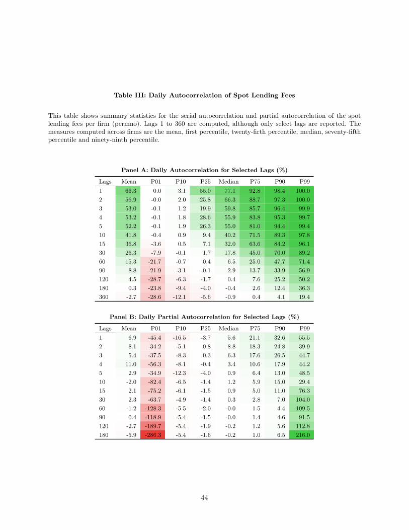
Table III: Daily Autocorrelation of Spot Lending Fees

This table shows summary statistics for the serial autocorrelation and partial autocorrelation of the spotlending fees per firm (permno). Lags 1 to 360 are computed, although only select lags are reported. Themeasures computed across firms are the mean, first percentile, twenty-firth percentile, median, seventy-fifthpercentile and ninety-ninth percentile.

Panel A: Daily Autocorrelation for Selected Lags (%)

Lags Mean P01 P10 P25 Median P75 P90 P991 66.3 0.0 3.1 55.0 77.1 92.8 98.4 100.02 56.9 -0.0 2.0 25.8 66.3 88.7 97.3 100.03 53.0 -0.1 1.2 19.9 59.8 85.7 96.4 99.94 53.2 -0.1 1.8 28.6 55.9 83.8 95.3 99.75 52.2 -0.1 1.9 26.3 55.0 81.0 94.4 99.410 41.8 -0.4 0.9 9.4 40.2 71.5 89.3 97.815 36.8 -3.6 0.5 7.1 32.0 63.6 84.2 96.130 26.3 -7.9 -0.1 1.7 17.8 45.0 70.0 89.260 15.3 -21.7 -0.7 0.4 6.5 25.0 47.7 71.490 8.8 -21.9 -3.1 -0.1 2.9 13.7 33.9 56.9120 4.5 -28.7 -6.3 -1.7 0.4 7.6 25.2 50.2180 0.3 -23.8 -9.4 -4.0 -0.4 2.6 12.4 36.3360 -2.7 -28.6 -12.1 -5.6 -0.9 0.4 4.1 19.4

Panel B: Daily Partial Autocorrelation for Selected Lags (%)

Lags Mean P01 P10 P25 Median P75 P90 P991 6.9 -45.4 -16.5 -3.7 5.6 21.1 32.6 55.52 8.1 -34.2 -5.1 0.8 8.8 18.3 24.8 39.93 5.4 -37.5 -8.3 0.3 6.3 17.6 26.5 44.74 11.0 -56.3 -8.1 -0.4 3.4 10.6 17.9 44.25 2.9 -34.9 -12.3 -4.0 0.9 6.4 13.0 48.510 -2.0 -82.4 -6.5 -1.4 1.2 5.9 15.0 29.415 2.1 -75.2 -6.1 -1.5 0.9 5.0 11.0 76.330 2.3 -63.7 -4.9 -1.4 0.3 2.8 7.0 104.060 -1.2 -128.3 -5.5 -2.0 -0.0 1.5 4.4 109.590 0.4 -118.9 -5.4 -1.5 -0.0 1.4 4.6 91.5120 -2.7 -189.7 -5.4 -1.9 -0.2 1.2 5.6 112.8180 -5.9 -286.3 -5.4 -1.6 -0.2 1.0 6.5 216.0

44

Table IV: Specialness Persistence Conditional on Jump Between Categories

This table shows the transition matrix between different special categories (proxied by DCBS from Markit)conditional on a previous jump from any to any category. Panel A shows the likelihood to end up in theDCBS at the top of each column after one trading day; Panel B, after 10 days; Panel C, after 20 days. Thelast line of each panel considers a jump from DCBS 1 to any DCBS greater than 1. The column titled “N”indicates the number of observations of each scenario.

Panel A: Conditional Transition Matrix After One PeriodJump to N →1 →2 →3 →4 →5 →6 →7 →8 →9 →101 8,118 78.9 19.9 1.0 0.1 0.0 0.0 0.0 0.0 0.0 0.02 9,987 33.2 58.6 7.3 0.6 0.1 0.0 0.0 0.0 0.0 0.03 4,109 7.3 21.1 60.7 9.5 1.1 0.2 0.0 0.0 0.0 0.04 2,367 3.2 3.2 19.1 61.2 11.4 1.6 0.3 0.1 0.0 0.05 1,645 2.1 2.1 2.0 16.7 61.8 13.2 1.8 0.2 0.1 0.16 1,372 1.0 0.4 1.2 3.1 15.2 65.0 12.8 0.7 0.4 0.17 1,192 0.9 0.3 0.2 0.2 1.8 13.8 69.5 11.2 1.8 0.38 955 0.6 0.2 0.1 0.1 0.0 1.7 15.8 66.3 13.7 1.59 777 0.8 0.0 0.5 0.3 0.4 0.8 1.3 14.8 68.1 13.110 373 0.8 0.3 0.5 0.3 0.0 0.3 0.8 1.1 19.6 76.4

Panel B: Conditional Transition Matrix After 10 PeriodsJump to N →1 →2 →3 →4 →5 →6 →7 →8 →9 →101 8,054 72.1 24.7 2.5 0.4 0.1 0.1 0.0 0.0 0.0 0.02 9,898 54.9 34.8 8.9 1.1 0.2 0.1 0.0 0.0 0.0 0.03 4,071 20.0 28.8 36.4 10.8 2.0 1.2 0.3 0.2 0.1 0.14 2,347 8.1 8.0 26.5 35.9 11.9 5.4 2.6 0.9 0.5 0.45 1,637 4.2 3.8 7.4 24.9 33.8 15.3 6.7 2.0 0.9 1.06 1,365 3.2 1.8 3.7 7.6 22.3 34.4 17.8 4.5 2.6 2.17 1,180 2.3 1.3 1.8 2.7 6.6 20.7 38.9 14.0 7.4 4.48 939 1.9 0.6 0.7 1.4 2.0 6.1 25.1 32.6 21.4 8.19 769 3.0 0.9 0.4 0.9 0.9 2.3 8.3 19.8 38.0 25.510 369 3.8 0.3 0.5 0.5 1.1 0.8 1.9 7.0 26.0 58.0

Panel C: Conditional Transition Matrix After 20 PeriodsJump to N →1 →2 →3 →4 →5 →6 →7 →8 →9 →101 7,988 73.5 22.6 2.8 0.6 0.3 0.2 0.1 0.0 0.0 0.02 9,807 58.1 31.4 7.9 1.6 0.5 0.2 0.2 0.1 0.1 0.03 4,033 24.0 30.1 30.0 9.9 2.5 1.5 1.1 0.4 0.3 0.24 2,332 11.2 10.0 25.9 30.0 10.1 6.0 3.7 1.5 1.1 0.65 1,626 6.0 5.5 9.4 26.6 23.5 14.6 7.8 2.7 2.1 1.86 1,353 4.0 3.8 5.2 12.9 20.0 25.5 14.3 6.9 4.5 2.87 1,173 3.4 2.0 3.6 4.8 8.6 19.9 27.5 15.5 8.1 6.68 928 2.3 1.3 2.5 1.8 3.8 7.8 25.1 25.8 17.0 12.79 759 3.2 1.8 0.9 1.4 1.7 3.4 12.4 17.1 32.3 25.710 365 4.9 0.5 1.4 0.5 1.1 2.2 4.4 8.2 28.2 48.5

45

Table V: Specialness Persistence Conditional on Jump from General Collateral to Special

This table shows the transition matrix between different special categories (proxied by DCBS from Markit)conditional on a previous jump from general collateral (DCBS 1) to the DCBS indicated on each line (from2 to 10). Panel A shows the likelihood to end up in the DCBS at the top of each column after one tradingday; Panel B, after 10 days; Panel C, after 20 days. The last line of each panel considers a jump from DCBS1 to any DCBS greater than 1. The column titled “N” indicates the number of observations of each scenario.

Panel A: Conditional Transition Matrix After One PeriodJump to N →1 →2 →3 →4 →5 →6 →7 →8 →9 →102 7,495 40.9 55.7 2.7 0.6 0.1 0.0 0.0 0.0 0.0 0.03 458 38.6 19.9 35.2 5.7 0.7 0.0 0.0 0.0 0.0 0.04 82 36.6 11.0 9.8 35.4 4.9 2.4 0.0 0.0 0.0 0.05 27 33.3 3.7 11.1 11.1 18.5 7.4 7.4 3.7 0.0 3.76 23 30.4 8.7 0.0 8.7 8.7 26.1 13.0 0.0 4.3 0.07 10 40.0 10.0 0.0 0.0 0.0 0.0 40.0 10.0 0.0 0.08 5 80.0 0.0 0.0 0.0 0.0 0.0 0.0 0.0 20.0 0.09 10 50.0 0.0 10.0 0.0 0.0 10.0 0.0 10.0 20.0 0.010 4 75.0 0.0 0.0 0.0 0.0 0.0 0.0 0.0 0.0 25.02 or more 8,114 40.7 52.8 4.6 1.3 0.2 0.1 0.1 0.0 0.1 0.0

Panel B: Conditional Transition Matrix After 10 PeriodsJump to N →1 →2 →3 →4 →5 →6 →7 →8 →9 →102 7,425 66.2 29.5 3.4 0.6 0.2 0.1 0.0 0.0 0.0 0.03 452 75.4 14.2 8.8 0.9 0.2 0.0 0.4 0.0 0.0 0.04 83 74.7 13.3 6.0 2.4 0.0 2.4 0.0 0.0 0.0 1.25 27 81.5 7.4 0.0 0.0 7.4 3.7 0.0 0.0 0.0 0.06 23 87.0 4.3 0.0 0.0 0.0 8.7 0.0 0.0 0.0 0.07 9 77.8 11.1 0.0 0.0 0.0 0.0 0.0 0.0 11.1 0.08 5 100.0 0.0 0.0 0.0 0.0 0.0 0.0 0.0 0.0 0.09 10 80.0 10.0 0.0 0.0 0.0 0.0 0.0 0.0 10.0 0.010 4 100.0 0.0 0.0 0.0 0.0 0.0 0.0 0.0 0.0 0.02 or more 8,038 67.0 28.2 3.7 0.6 0.2 0.1 0.0 0.0 0.0 0.0

Panel C: Conditional Transition Matrix After 20 PeriodsJump to N →1 →2 →3 →4 →5 →6 →7 →8 →9 →102 7,366 68.4 26.5 3.4 1.0 0.3 0.2 0.2 0.0 0.0 0.03 452 76.5 15.0 6.4 1.1 0.4 0.2 0.2 0.0 0.0 0.04 83 75.9 9.6 7.2 3.6 1.2 1.2 0.0 0.0 0.0 1.25 27 74.1 11.1 7.4 0.0 0.0 7.4 0.0 0.0 0.0 0.06 23 73.9 13.0 4.3 0.0 4.3 0.0 0.0 4.3 0.0 0.07 10 90.0 0.0 0.0 0.0 0.0 0.0 0.0 0.0 10.0 0.08 5 100.0 0.0 0.0 0.0 0.0 0.0 0.0 0.0 0.0 0.09 10 60.0 30.0 0.0 0.0 0.0 0.0 10.0 0.0 0.0 0.010 4 100.0 0.0 0.0 0.0 0.0 0.0 0.0 0.0 0.0 0.02 or more 7,980 69.1 25.5 3.6 1.0 0.3 0.2 0.2 0.0 0.0 0.0

46

Table VI: Summary Statistics of the Estimated Implied Lending Fee by Maturity and Special-ness

This table shows the summary statistics for the estimated implied lending fee by maturity range (Panel A)and specialness (Panel B). The measures reported are the mean, median, first percentile, tenth percentile,twenty-firth percentile, seventy-fifth percentile, ninetieth percentile, and ninety-ninth percentile. All measuresare in percent. Panel C shows the median across maturity and specialness.

Panel A: Implied Lending Fee by Maturity (%)

Maturity Mean P01 P10 P25 Median P75 P90 P99Less than 7 60.2 -14.4 3.6 12.1 31.4 79.0 177.4 396.38 to 15 25.0 -2.8 1.9 4.9 11.3 26.0 60.3 200.016 to 30 14.2 -1.6 0.9 2.5 5.9 13.7 32.1 156.631 to 60 8.9 -1.0 0.5 1.5 3.5 8.2 19.7 98.261 to 90 5.4 -1.2 0.1 0.7 1.9 4.8 12.1 62.691 to 180 4.0 -1.3 0.1 0.5 1.4 3.6 9.2 46.1181 to 360 3.1 -1.6 -0.1 0.3 1.0 2.8 7.2 35.4More than 361 3.5 -1.0 0.1 0.6 1.5 3.2 7.2 35.7All 10.0 -1.7 0.1 0.8 2.4 7.3 21.8 155.9

Panel B: Implied Lending Fee by Specialness (%)

DCBS Mean P01 P10 P25 Median P75 P90 P991 7.5 -1.9 0.1 0.7 2.0 5.5 15.2 112.82 17.9 -0.5 1.1 2.6 6.2 15.5 40.6 200.03 24.2 -0.1 2.3 4.9 9.8 22.3 56.3 200.04 28.1 0.7 4.2 7.3 13.2 27.5 64.9 200.05 30.0 1.4 5.7 9.0 15.2 30.0 67.6 200.06 33.1 1.6 6.6 10.7 17.8 33.4 73.2 201.17 41.8 2.1 8.8 13.9 22.9 43.5 97.0 256.08 52.6 3.8 11.3 17.4 28.7 59.2 136.0 318.59 58.3 5.1 14.6 22.7 37.1 68.0 136.6 298.010 86.5 8.7 21.8 34.9 61.2 115.3 200.0 390.0All 10.0 -1.7 0.1 0.8 2.4 7.3 21.8 155.9

Panel C: Median Implied Lending Fee by Maturity and Specialness (%)

Mat.\DCBS 1 2 3 4 5 6 7 8 9 10Less than 7 27.4 70.9 84.4 99.2 100.5 98.6 121.0 151.4 167.9 200.08 to 15 9.8 25.9 34.7 41.1 40.7 45.6 57.9 73.8 87.8 144.816 to 30 5.0 14.4 20.2 25.2 25.5 29.0 38.5 52.7 64.7 109.331 to 60 3.0 9.0 13.4 17.3 19.3 22.1 29.7 38.0 48.7 81.161 to 90 1.6 5.6 8.9 12.3 14.8 17.3 23.0 28.3 37.8 60.191 to 180 1.2 4.3 7.1 10.1 12.0 14.3 18.9 23.2 30.6 47.2181 to 360 0.8 3.4 6.0 8.1 9.6 11.6 15.7 18.9 24.6 37.3≥ 361 1.3 3.5 5.7 7.5 8.8 10.0 12.7 14.9 18.9 30.8

47

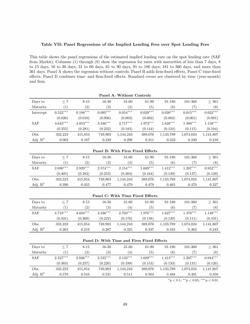
Table VII: Panel Regressions of the Implied Lending Fees over Spot Lending Fees

This table shows the panel regressions of the estimated implied lending rate on the spot lending rate (SAFfrom Markit). Columns (1) through (8) show the regression for rates with maturities of less than 7 days, 8to 15 days, 16 to 30 days, 31 to 60 days, 61 to 90 days, 91 to 180 days, 181 to 360 days, and more than361 days. Panel A shows the regression without controls. Panel B adds firm-fixed effects, Panel C time-fixedeffects. Panel D combines time- and firm-fixed effects. Standard errors are clustered by time (year-month)and firm.

Panel A: Without ControlsDays to ≤ 7 8-15 16-30 31-60 61-90 91-180 181-360 ≥ 361Maturity (1) (2) (3) (4) (5) (6) (7) (8)Intercept 0.522∗∗∗ 0.188∗∗∗ 0.095∗∗∗ 0.054∗∗∗ 0.029∗∗∗ 0.020∗∗∗ 0.015∗∗∗ 0.022∗∗∗

(0.026) (0.010) (0.006) (0.003) (0.002) (0.002) (0.001) (0.001)SAF 4.643∗∗∗ 4.053∗∗∗ 3.346∗∗∗ 2.717∗∗∗ 1.973∗∗∗ 1.628∗∗∗ 1.380∗∗∗ 1.158∗∗∗

(0.355) (0.281) (0.232) (0.183) (0.144) (0.124) (0.115) (0.104)Obs. 332,223 415,854 749,903 1,144,243 389,076 1,133,789 1,074,024 1,141,807Adj. R2 0.063 0.167 0.249 0.296 0.311 0.322 0.340 0.210

Panel B: With Firm Fixed EffectsDays to ≤ 7 8-15 16-30 31-60 61-90 91-180 181-360 ≥ 361Maturity (1) (2) (3) (4) (5) (6) (7) (8)SAF 2.690∗∗∗ 2.929∗∗∗ 2.574∗∗∗ 2.154∗∗∗ 1.689∗∗∗ 1.412∗∗∗ 1.207∗∗∗ 0.952∗∗∗

(0.405) (0.282) (0.253) (0.204) (0.164) (0.139) (0.137) (0.129)Obs. 332,223 415,854 749,903 1,144,243 389,076 1,133,789 1,074,024 1,141,807Adj. R2 0.390 0.455 0.477 0.479 0.479 0.465 0.470 0.327

Panel C: With Time Fixed EffectsDays to ≤ 7 8-15 16-30 31-60 61-90 91-180 181-360 ≥ 361Maturity (1) (2) (3) (4) (5) (6) (7) (8)SAF 4.718∗∗∗ 4.034∗∗∗ 3.336∗∗∗ 2.703∗∗∗ 1.976∗∗∗ 1.627∗∗∗ 1.378∗∗∗ 1.148∗∗∗

(0.331) (0.269) (0.222) (0.176) (0.138) (0.120) (0.111) (0.101)Obs. 332,223 415,854 749,903 1,144,243 389,076 1,133,789 1,074,024 1,141,807Adj. R2 0.263 0.219 0.287 0.325 0.337 0.345 0.362 0.243

Panel D: With Time and Firm Fixed EffectsDays to ≤ 7 8-15 16-30 31-60 61-90 91-180 181-360 ≥ 361Maturity (1) (2) (3) (4) (5) (6) (7) (8)SAF 2.527∗∗∗ 2.826∗∗∗ 2.535∗∗∗ 2.133∗∗∗ 1.689∗∗∗ 1.413∗∗∗ 1.207∗∗∗ 0.944∗∗∗

(0.363) (0.257) (0.226) (0.189) (0.153) (0.133) (0.131) (0.126)Obs. 332,223 415,854 749,903 1,144,243 389,076 1,133,789 1,074,024 1,141,807Adj. R2 0.579 0.516 0.521 0.511 0.504 0.488 0.491 0.358

∗p < 0.1; ∗∗p < 0.05; ∗∗∗p < 0.01

48

Table VIII: Summary Statistics of the Estimated Volatility by Maturity and Specialness

This table shows the summary statistics for the estimated implied volatility by maturity range (Panel A)and specialness (Panel B). The measures reported are the mean, median, first percentile, tenth percentile,twenty-firth percentile, seventy-fifth percentile, ninetieth percentile, and ninety-ninth percentile. Panel Cshows the median across maturity and specialness.

Panel A: Volatility by Maturity (%)

Maturity Mean P01 P10 P25 Median P75 P90 P99Less than 7 40.94 10.73 17.07 22.93 33.11 49.23 73.31 153.858 to 15 39.31 11.14 16.94 22.80 32.65 47.74 68.90 136.2616 to 30 39.33 11.54 17.29 23.29 33.21 47.85 68.01 130.5131 to 60 41.07 12.39 18.60 24.81 35.00 49.58 70.06 133.9761 to 90 41.72 12.94 19.09 25.18 35.41 50.15 71.51 136.7691 to 180 42.22 13.62 20.25 26.42 36.60 50.45 70.51 132.38181 to 360 41.28 14.13 20.63 26.52 36.08 49.12 68.01 124.00More than 361 41.21 14.80 21.82 27.60 36.57 48.53 65.90 116.48All 41.06 12.59 19.34 25.54 35.41 49.18 68.94 130.04

Panel B: Volatility by Specialness (%)

DCBS Mean P01 P10 P25 Median P75 P90 P991 37.65 12.51 18.90 24.67 33.50 45.14 60.38 109.452 57.28 14.15 26.96 38.37 52.66 69.41 91.74 160.063 64.50 11.86 31.87 44.55 58.80 77.57 103.47 177.404 69.64 12.40 36.33 48.19 64.02 83.06 109.05 189.495 71.83 24.84 40.75 50.74 64.59 84.07 111.62 192.676 74.75 25.28 42.31 52.27 67.24 88.67 114.77 202.517 77.42 28.15 43.96 53.95 68.91 91.43 122.42 203.758 82.33 28.31 45.99 56.57 73.42 100.51 129.10 208.799 87.19 28.47 47.79 59.77 78.89 105.94 135.96 220.6610 96.96 27.23 56.04 70.45 88.98 114.26 148.64 225.96All 41.06 12.59 19.34 25.54 35.41 49.18 68.94 130.04

Panel C: Median Volatility by Maturity and Specialness (%)

Mat.\DCBS 1 2 3 4 5 6 7 8 9 10Less than 7 31.0 52.9 58.4 63.7 64.2 67.6 67.7 71.3 75.1 89.68 to 15 30.6 51.2 56.8 61.8 62.0 66.5 67.5 70.5 75.5 87.916 to 30 31.1 51.6 56.7 61.6 62.3 65.9 66.1 70.9 77.0 86.631 to 60 32.9 52.9 59.1 64.2 64.3 68.0 68.2 72.7 80.1 88.461 to 90 33.4 53.4 60.6 67.8 66.1 69.9 72.9 76.3 81.9 90.991 to 180 34.6 53.8 59.9 65.7 66.9 69.7 70.6 75.6 80.7 90.1181 to 360 34.3 52.1 58.9 64.0 65.3 64.6 69.3 72.0 77.1 88.8≥ 361 35.1 52.6 58.9 63.3 64.1 66.7 68.3 75.7 79.6 89.6

49

Table IX: Panel Regressions of the Implied Lending Fees over Implied Volatility

This table shows the panel regressions of the estimated implied lending rate to the implied volatility rate.Columns (1) through (8) show the regression for rates with maturities of less than 7 days, 8 to 15 days, 16to 30 days, 31 to 60 days, 61 to 90 days, 91 to 180 days, 181 to 360 days, and more than 361 days. Panel Ashows the regression without controls. Panel B adds firm-fixed effects, Panel C time-fixed effects. Panel Dcombines time- and firm-fixed effects. Standard errors are clustered by time (year-month) and firm.

Panel A: Without ControlsDays to ≤ 7 8-15 16-30 31-60 61-90 91-180 181-360 ≥ 361Maturity (1) (2) (3) (4) (5) (6) (7) (8)Intercept 0.053∗∗ −0.096∗∗∗ −0.099∗∗∗ −0.082∗∗∗ −0.069∗∗∗ −0.060∗∗∗ −0.054∗∗∗ −0.055∗∗∗

(0.021) (0.012) (0.012) (0.010) (0.006) (0.006) (0.006) (0.007)Impl. Vol. 1.341∗∗∗ 0.880∗∗∗ 0.614∗∗∗ 0.415∗∗∗ 0.296∗∗∗ 0.237∗∗∗ 0.205∗∗∗ 0.217∗∗∗

(0.061) (0.043) (0.041) (0.032) (0.021) (0.017) (0.019) (0.020)Obs. 357,250 457,237 826,527 1,284,417 440,277 1,300,282 1,223,607 1,268,939Adj. R2 0.257 0.288 0.276 0.257 0.284 0.264 0.260 0.221

Panel B: With Firm Fixed EffectsDays to ≤ 7 8-15 16-30 31-60 61-90 91-180 181-360 ≥ 361Maturity (1) (2) (3) (4) (5) (6) (7) (8)Impl. Vol. 0.975∗∗∗ 0.662∗∗∗ 0.460∗∗∗ 0.311∗∗∗ 0.243∗∗∗ 0.199∗∗∗ 0.179∗∗∗ 0.212∗∗∗

(0.063) (0.036) (0.031) (0.025) (0.020) (0.019) (0.024) (0.026)Obs. 357,250 457,237 826,527 1,284,417 440,277 1,300,282 1,223,607 1,268,939Adj. R2 0.466 0.496 0.472 0.443 0.437 0.413 0.414 0.347

Panel C: With Time Fixed EffectsDays to ≤ 7 8-15 16-30 31-60 61-90 91-180 181-360 ≥ 361Maturity (1) (2) (3) (4) (5) (6) (7) (8)Impl. Vol. 1.308∗∗∗ 0.941∗∗∗ 0.685∗∗∗ 0.487∗∗∗ 0.341∗∗∗ 0.275∗∗∗ 0.239∗∗∗ 0.249∗∗∗

(0.065) (0.048) (0.042) (0.033) (0.022) (0.018) (0.020) (0.020)Obs. 357,250 457,237 826,527 1,284,417 440,277 1,300,282 1,223,607 1,268,939Adj. R2 0.398 0.320 0.312 0.302 0.320 0.306 0.310 0.279

Panel D: With Time and Firm Fixed EffectsDays to ≤ 7 8-15 16-30 31-60 61-90 91-180 181-360 ≥ 361Maturity (1) (2) (3) (4) (5) (6) (7) (8)Impl. Vol. 0.771∗∗∗ 0.657∗∗∗ 0.511∗∗∗ 0.390∗∗∗ 0.315∗∗∗ 0.277∗∗∗ 0.266∗∗∗ 0.304∗∗∗

(0.065) (0.045) (0.039) (0.035) (0.031) (0.028) (0.034) (0.033)Obs. 357,250 457,237 826,527 1,284,417 440,277 1,300,282 1,223,607 1,268,939Adj. R2 0.605 0.529 0.500 0.470 0.460 0.443 0.455 0.400

∗p < 0.1; ∗∗p < 0.05; ∗∗∗p < 0.01

50

Table X: Panel Regressions of the Implied Lending Fees over Spot Lending Rate and ImpliedVolatility

This table shows the panel regressions of the estimated implied lending rate to the spot lending rate andimplied volatility rate. Columns (1) through (8) show the regression for implied rates with maturities of lessthan 7 days, 8 to 15 days, 16 to 30 days, 31 to 60 days, 61 to 90 days, 91 to 180 days, 181 to 360 days, andmore than 361 days. Panel A shows the regression without controls. Panel B time- and firm-fixed effects.Panel C combines a number of controls and time- and firm-fixed effects. Standard errors are clustered bytime (year-month) and firm.

Panel A: Without ControlsDays to ≤ 7 8-15 16-30 31-60 61-90 91-180 181-360 ≥ 361Maturity (1) (2) (3) (4) (5) (6) (7) (8)Intercept 0.068∗∗∗ −0.060∗∗∗ −0.065∗∗∗ −0.056∗∗∗ −0.051∗∗∗ −0.043∗∗∗ −0.039∗∗∗ −0.038∗∗∗

(0.023) (0.012) (0.009) (0.007) (0.005) (0.005) (0.005) (0.006)SAF 1.940∗∗∗ 2.535∗∗∗ 2.415∗∗∗ 2.104∗∗∗ 1.502∗∗∗ 1.282∗∗∗ 1.095∗∗∗ 0.850∗∗∗

(0.224) (0.224) (0.199) (0.159) (0.120) (0.107) (0.102) (0.084)Impl. Vol. 1.208∗∗∗ 0.693∗∗∗ 0.448∗∗∗ 0.293∗∗∗ 0.211∗∗∗ 0.165∗∗∗ 0.141∗∗∗ 0.156∗∗∗

(0.072) (0.043) (0.034) (0.025) (0.017) (0.014) (0.015) (0.016)Obs. 332,223 415,854 749,903 1,144,243 389,076 1,133,789 1,074,024 1,141,807Adj. R2 0.252 0.327 0.379 0.408 0.441 0.435 0.444 0.309

Panel B: With Time and Firm Fixed EffectsDays to ≤ 7 8-15 16-30 31-60 61-90 91-180 181-360 ≥ 361Maturity (1) (2) (3) (4) (5) (6) (7) (8)SAF 1.733∗∗∗ 2.188∗∗∗ 2.094∗∗∗ 1.802∗∗∗ 1.411∗∗∗ 1.199∗∗∗ 0.996∗∗∗ 0.702∗∗∗

(0.279) (0.199) (0.187) (0.158) (0.124) (0.108) (0.100) (0.079)Impl. Vol. 0.689∗∗∗ 0.520∗∗∗ 0.380∗∗∗ 0.295∗∗∗ 0.247∗∗∗ 0.221∗∗∗ 0.215∗∗∗ 0.253∗∗∗

(0.067) (0.045) (0.033) (0.028) (0.026) (0.025) (0.030) (0.033)Obs. 332,223 415,854 749,903 1,144,243 389,076 1,133,789 1,074,024 1,141,807Adj. R2 0.608 0.552 0.555 0.548 0.557 0.544 0.557 0.434

∗p < 0.1; ∗∗p < 0.05; ∗∗∗p < 0.01

51

Table X (cont.): Panel Regressions of the Implied Lending Fees over Spot Lending Rate andImplied Volatility

Panel C: With Controls but No Fixed EffectsDays to ≤ 7 8-15 16-30 31-60 61-90 91-180 181-360 ≥ 361Maturity (1) (2) (3) (4) (5) (6) (7) (8)Intercept 4.024∗∗∗ 1.670∗∗∗ 0.770∗∗∗ 0.397∗∗∗ 0.220∗∗∗ 0.133∗∗∗ 0.074∗∗∗ 0.020

(0.240) (0.143) (0.091) (0.058) (0.039) (0.028) (0.027) (0.037)SAF 1.354∗∗∗ 2.315∗∗∗ 2.324∗∗∗ 2.053∗∗∗ 1.493∗∗∗ 1.266∗∗∗ 1.093∗∗∗ 0.841∗∗∗

(0.234) (0.231) (0.213) (0.170) (0.129) (0.117) (0.112) (0.096)Impl. Vol. 0.770∗∗∗ 0.497∗∗∗ 0.364∗∗∗ 0.270∗∗∗ 0.201∗∗∗ 0.160∗∗∗ 0.144∗∗∗ 0.167∗∗∗

(0.080) (0.046) (0.035) (0.027) (0.020) (0.017) (0.020) (0.025)RV (20 days) 0.200∗ −0.066 −0.089∗∗ −0.110∗∗∗ −0.066∗∗∗ −0.053∗∗∗ −0.054∗∗∗ −0.046∗∗∗

(0.110) (0.055) (0.036) (0.028) (0.018) (0.015) (0.017) (0.016)Utilization −0.002∗∗∗ −0.001∗∗∗ −0.001∗∗∗ −0.001∗∗∗ −0.001∗∗∗ −0.0003∗∗∗ −0.0003∗∗∗ −0.0003∗∗∗

(0.001) (0.0004) (0.0003) (0.0002) (0.0001) (0.0001) (0.0001) (0.0001)Available Ratio −0.129 −0.234∗∗∗ −0.156∗∗∗ −0.098∗∗∗ −0.061∗∗∗ −0.036∗∗ −0.026∗∗ −0.035∗∗∗

(0.162) (0.089) (0.057) (0.034) (0.021) (0.015) (0.011) (0.014)Avg. Tenure 0.001∗∗∗ 0.0003∗∗∗ 0.0002∗∗∗ 0.0001∗∗∗ 0.0001∗∗∗ 0.00005∗∗∗ 0.00004∗∗∗ 0.00004∗∗∗

(0.0001) (0.0001) (0.0001) (0.00004) (0.00002) (0.00001) (0.00001) (0.00001)Inv. Concentr. 0.455∗∗ 0.318∗∗∗ 0.247∗∗∗ 0.166∗∗∗ 0.084∗∗∗ 0.059∗∗∗ 0.050∗∗∗ 0.071∗∗∗

(0.207) (0.108) (0.073) (0.046) (0.021) (0.016) (0.013) (0.020)Loan Concentr. 0.120∗∗ 0.030 0.016 0.005 0.001 0.002 0.004 −0.003

(0.047) (0.024) (0.015) (0.009) (0.006) (0.004) (0.004) (0.004)Demand Concentr. −0.006 0.009 −0.004 −0.003 −0.004 0.001 −0.002 −0.001

(0.040) (0.024) (0.016) (0.010) (0.007) (0.005) (0.004) (0.004)Log(Mkt. Cap.) −0.166∗∗∗ −0.071∗∗∗ −0.034∗∗∗ −0.018∗∗∗ −0.011∗∗∗ −0.007∗∗∗ −0.005∗∗∗ −0.002∗

(0.009) (0.005) (0.003) (0.002) (0.001) (0.001) (0.001) (0.001)Obs. 332,073 415,599 749,432 1,143,411 388,743 1,132,945 1,073,309 1,141,231Adj. R2 0.340 0.386 0.415 0.436 0.461 0.451 0.458 0.320

∗p<0.1; ∗∗p<0.05; ∗∗∗p<0.01

52

Table XI: Summary Statistics of the Lending Fee and Volatility Risk Premia by Maturity

This table shows the median lending fee and volatility risk premia for each maturity range. The risk premiaare computed as the difference between the implied risk premium and the realized risk premium until thematurity. The measures reported are the mean, median, first percentile, twenty-firth percentile, seventy-fifthpercentile and ninety-ninth percentile.

Panel A: Lending Fee Risk Premia

Maturity (days) Mean P01 P10 P25 Median P75 P90 P99Less than 7 0.56 -0.15 0.03 0.11 0.29 0.73 1.66 3.648 to 15 0.22 -0.03 0.01 0.04 0.10 0.23 0.53 1.9316 to 30 0.12 -0.02 0.01 0.02 0.05 0.12 0.27 1.3531 to 60 0.07 -0.02 0.00 0.01 0.03 0.07 0.16 0.8061 to 90 0.04 -0.03 0.00 0.00 0.01 0.04 0.09 0.4691 to 180 0.03 -0.05 0.00 0.00 0.01 0.03 0.07 0.33181 to 360 0.02 -0.06 0.00 0.00 0.01 0.02 0.05 0.26More than 361 0.02 -0.08 0.00 0.00 0.01 0.03 0.06 0.27All 0.08 -0.05 0.00 0.00 0.02 0.06 0.18 1.39

Panel B: Volatility Risk Premia

Maturity (days) Mean P01 P10 P25 Median P75 P90 P99Less than 7 0.26 -0.14 0.11 0.04 0.20 0.35 0.56 1.328 to 15 0.23 -0.15 0.09 0.03 0.18 0.31 0.49 1.0916 to 30 0.22 -0.18 0.09 0.02 0.18 0.31 0.48 1.0531 to 60 0.23 -0.18 0.09 0.03 0.19 0.31 0.49 1.0861 to 90 0.23 -0.18 0.09 0.03 0.19 0.31 0.49 1.1191 to 180 0.23 -0.24 0.09 0.02 0.19 0.31 0.49 1.08181 to 360 0.22 -0.21 0.08 0.01 0.18 0.30 0.48 1.03More than 361 0.23 -0.11 0.10 0.04 0.19 0.30 0.46 0.96All 0.23 -0.18 0.09 0.02 0.18 0.31 0.49 1.06

53

Table XII: Summary Statistics of the Lending Fee and Volatility Risk Premia by Specialness

This table shows the median lending fee and volatility risk premia for specialness category. Specialness isproxied by DCBS from Markit. The risk premia are computed as the difference between the implied riskpremium and the realized risk premium until the maturity. The measures reported are the mean, median,first percentile, twenty-firth percentile, seventy-fifth percentile and ninety-ninth percentile.

Panel A: Lending Fee Risk Premia

DCBS Mean P01 P10 P25 Median P75 P90 P991 0.07 -0.03 0.00 0.00 0.02 0.05 0.14 1.032 0.15 -0.07 0.00 0.01 0.04 0.13 0.36 1.983 0.20 -0.10 -0.01 0.02 0.06 0.18 0.50 1.974 0.22 -0.15 -0.01 0.03 0.08 0.22 0.58 1.965 0.21 -0.16 -0.02 0.02 0.08 0.21 0.57 1.936 0.22 -0.19 -0.04 0.01 0.08 0.22 0.60 1.937 0.28 -0.20 -0.03 0.02 0.11 0.29 0.81 2.278 0.35 -0.19 -0.04 0.03 0.14 0.41 1.13 2.699 0.38 -0.19 -0.03 0.05 0.18 0.46 1.12 2.6310 0.54 -0.25 -0.03 0.10 0.31 0.77 1.53 3.39All 0.08 -0.05 0.00 0.00 0.02 0.06 0.18 1.39

Panel B: Volatility Risk Premia

DCBS Mean P01 P10 P25 Median P75 P90 P991 0.07 -0.03 0.00 0.00 0.02 0.05 0.14 1.032 0.15 -0.07 0.00 0.01 0.04 0.13 0.36 1.983 0.20 -0.10 -0.01 0.02 0.06 0.18 0.50 1.974 0.22 -0.15 -0.01 0.03 0.08 0.22 0.58 1.965 0.21 -0.16 -0.02 0.02 0.08 0.21 0.57 1.936 0.22 -0.19 -0.04 0.01 0.08 0.22 0.60 1.937 0.28 -0.20 -0.03 0.02 0.11 0.29 0.81 2.278 0.35 -0.19 -0.04 0.03 0.14 0.41 1.13 2.699 0.38 -0.19 -0.03 0.05 0.18 0.46 1.12 2.6310 0.54 -0.25 -0.03 0.10 0.31 0.77 1.53 3.39All 0.08 -0.05 0.00 0.00 0.02 0.06 0.18 1.39

54

Table XIII: Median Lending Fee and Volatility Risk Premia by Specialness and Maturity

This table shows the median lending fee and volatility risk premia for each maturity and specialness category.Specialness is proxied by DCBS from Markit. The risk premia are computed as the difference between theimplied risk premium and the realized risk premium until the maturity.

Panel A: Median Lending Fee Risk Premia

Mat. 1 2 3 4 5 6 7 8 9 10Less than 7 0.3 0.7 0.8 0.9 0.9 0.9 1.1 1.4 1.4 1.68 to 15 0.1 0.2 0.3 0.3 0.3 0.3 0.4 0.6 0.7 1.016 to 30 0.0 0.1 0.2 0.2 0.2 0.2 0.3 0.4 0.4 0.731 to 60 0.0 0.1 0.1 0.1 0.1 0.1 0.2 0.2 0.3 0.561 to 90 0.0 0.0 0.1 0.1 0.1 0.1 0.1 0.1 0.2 0.391 to 180 0.0 0.0 0.0 0.1 0.1 0.1 0.1 0.1 0.1 0.2181 to 360 0.0 0.0 0.0 0.0 0.0 0.0 0.1 0.1 0.1 0.2≥ 361 0.0 0.0 0.0 0.0 0.0 0.0 0.0 0.0 0.1 0.1

Panel B: Median Volatility Risk Premia

Mat. 1 2 3 4 5 6 7 8 9 10≤ 7 0.2 0.4 0.5 0.5 0.5 0.5 0.6 0.6 0.6 0.78 to 15 0.2 0.3 0.4 0.4 0.5 0.5 0.5 0.6 0.6 0.716 to 30 0.2 0.4 0.4 0.5 0.5 0.5 0.5 0.6 0.6 0.731 to 60 0.2 0.4 0.4 0.5 0.5 0.5 0.5 0.6 0.6 0.761 to 90 0.2 0.3 0.4 0.5 0.5 0.5 0.5 0.6 0.6 0.791 to 180 0.2 0.3 0.4 0.5 0.5 0.5 0.5 0.6 0.6 0.7181 to 360 0.2 0.3 0.4 0.5 0.5 0.5 0.5 0.5 0.6 0.7≥ 361 0.2 0.3 0.4 0.5 0.5 0.5 0.5 0.6 0.6 0.7

55

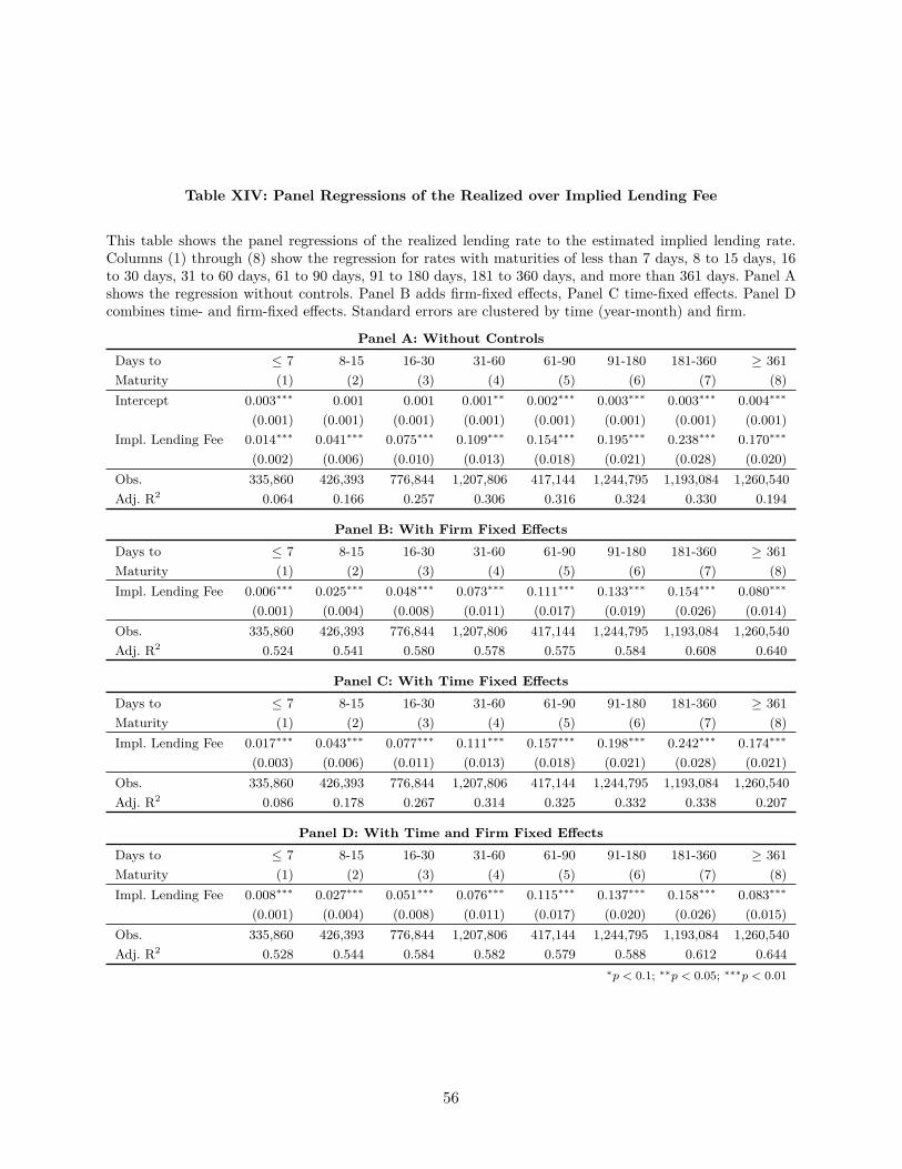
Table XIV: Panel Regressions of the Realized over Implied Lending Fee

This table shows the panel regressions of the realized lending rate to the estimated implied lending rate.Columns (1) through (8) show the regression for rates with maturities of less than 7 days, 8 to 15 days, 16to 30 days, 31 to 60 days, 61 to 90 days, 91 to 180 days, 181 to 360 days, and more than 361 days. Panel Ashows the regression without controls. Panel B adds firm-fixed effects, Panel C time-fixed effects. Panel Dcombines time- and firm-fixed effects. Standard errors are clustered by time (year-month) and firm.

Panel A: Without ControlsDays to ≤ 7 8-15 16-30 31-60 61-90 91-180 181-360 ≥ 361Maturity (1) (2) (3) (4) (5) (6) (7) (8)Intercept 0.003∗∗∗ 0.001 0.001 0.001∗∗ 0.002∗∗∗ 0.003∗∗∗ 0.003∗∗∗ 0.004∗∗∗

(0.001) (0.001) (0.001) (0.001) (0.001) (0.001) (0.001) (0.001)Impl. Lending Fee 0.014∗∗∗ 0.041∗∗∗ 0.075∗∗∗ 0.109∗∗∗ 0.154∗∗∗ 0.195∗∗∗ 0.238∗∗∗ 0.170∗∗∗

(0.002) (0.006) (0.010) (0.013) (0.018) (0.021) (0.028) (0.020)Obs. 335,860 426,393 776,844 1,207,806 417,144 1,244,795 1,193,084 1,260,540Adj. R2 0.064 0.166 0.257 0.306 0.316 0.324 0.330 0.194

Panel B: With Firm Fixed EffectsDays to ≤ 7 8-15 16-30 31-60 61-90 91-180 181-360 ≥ 361Maturity (1) (2) (3) (4) (5) (6) (7) (8)Impl. Lending Fee 0.006∗∗∗ 0.025∗∗∗ 0.048∗∗∗ 0.073∗∗∗ 0.111∗∗∗ 0.133∗∗∗ 0.154∗∗∗ 0.080∗∗∗

(0.001) (0.004) (0.008) (0.011) (0.017) (0.019) (0.026) (0.014)Obs. 335,860 426,393 776,844 1,207,806 417,144 1,244,795 1,193,084 1,260,540Adj. R2 0.524 0.541 0.580 0.578 0.575 0.584 0.608 0.640

Panel C: With Time Fixed EffectsDays to ≤ 7 8-15 16-30 31-60 61-90 91-180 181-360 ≥ 361Maturity (1) (2) (3) (4) (5) (6) (7) (8)Impl. Lending Fee 0.017∗∗∗ 0.043∗∗∗ 0.077∗∗∗ 0.111∗∗∗ 0.157∗∗∗ 0.198∗∗∗ 0.242∗∗∗ 0.174∗∗∗

(0.003) (0.006) (0.011) (0.013) (0.018) (0.021) (0.028) (0.021)Obs. 335,860 426,393 776,844 1,207,806 417,144 1,244,795 1,193,084 1,260,540Adj. R2 0.086 0.178 0.267 0.314 0.325 0.332 0.338 0.207

Panel D: With Time and Firm Fixed EffectsDays to ≤ 7 8-15 16-30 31-60 61-90 91-180 181-360 ≥ 361Maturity (1) (2) (3) (4) (5) (6) (7) (8)Impl. Lending Fee 0.008∗∗∗ 0.027∗∗∗ 0.051∗∗∗ 0.076∗∗∗ 0.115∗∗∗ 0.137∗∗∗ 0.158∗∗∗ 0.083∗∗∗

(0.001) (0.004) (0.008) (0.011) (0.017) (0.020) (0.026) (0.015)Obs. 335,860 426,393 776,844 1,207,806 417,144 1,244,795 1,193,084 1,260,540Adj. R2 0.528 0.544 0.584 0.582 0.579 0.588 0.612 0.644

∗p < 0.1; ∗∗p < 0.05; ∗∗∗p < 0.01

56

Table XV: Panel Regressions of the Realized over Implied Lending Fee and Volatility

This table shows the panel regressions of the realized lending rate to the estimated implied lending rate andthe implied volatility rate. Columns (1) through (8) show the regression for rates with maturities of lessthan 7 days, 8 to 15 days, 16 to 30 days, 31 to 60 days, 61 to 90 days, 91 to 180 days, 181 to 360 days, andmore than 361 days. Panel A shows the regression without controls. Panel B adds firm-fixed effects, PanelC time-fixed effects. Panel D combines time- and firm-fixed effects. Standard errors are clustered by time(year-month) and firm.

Panel A: Without ControlsDays to ≤ 7 8-15 16-30 31-60 61-90 91-180 181-360 ≥ 361Maturity (1) (2) (3) (4) (5) (6) (7) (8)Intercept −0.008∗∗∗ −0.009∗∗∗ −0.008∗∗∗ −0.005∗∗∗ −0.003∗∗ −0.003∗ −0.003∗ −0.009∗∗∗

(0.002) (0.002) (0.002) (0.002) (0.002) (0.002) (0.002) (0.003)Impl. Lending Fee 0.007∗∗∗ 0.030∗∗∗ 0.063∗∗∗ 0.098∗∗∗ 0.140∗∗∗ 0.179∗∗∗ 0.218∗∗∗ 0.131∗∗∗

(0.001) (0.005) (0.010) (0.012) (0.017) (0.021) (0.027) (0.016)Impl. Vol. 0.037∗∗∗ 0.033∗∗∗ 0.026∗∗∗ 0.018∗∗∗ 0.016∗∗∗ 0.015∗∗∗ 0.016∗∗∗ 0.036∗∗∗

(0.006) (0.006) (0.005) (0.005) (0.005) (0.005) (0.005) (0.009)Obs. 335,860 426,393 776,844 1,207,806 417,144 1,244,795 1,193,084 1,260,540Adj. R2 0.115 0.196 0.274 0.315 0.324 0.331 0.337 0.230

Panel B: With Firm Fixed EffectsDays to ≤ 7 8-15 16-30 31-60 61-90 91-180 181-360 ≥ 361Maturity (1) (2) (3) (4) (5) (6) (7) (8)Impl. Lending Fee 0.004∗∗∗ 0.021∗∗∗ 0.044∗∗∗ 0.069∗∗∗ 0.106∗∗∗ 0.130∗∗∗ 0.151∗∗∗ 0.072∗∗∗

(0.001) (0.004) (0.008) (0.011) (0.017) (0.020) (0.027) (0.013)Impl. Vol. 0.015∗∗∗ 0.016∗∗∗ 0.015∗∗∗ 0.012∗∗∗ 0.009∗ 0.006 0.005 0.013∗∗

(0.003) (0.005) (0.005) (0.004) (0.005) (0.004) (0.005) (0.006)Obs. 335,860 426,393 776,844 1,207,806 417,144 1,244,795 1,193,084 1,260,540Adj. R2 0.530 0.546 0.583 0.580 0.576 0.585 0.608 0.642

Panel C: With Time Fixed EffectsDays to ≤ 7 8-15 16-30 31-60 61-90 91-180 181-360 ≥ 361Maturity (1) (2) (3) (4) (5) (6) (7) (8)Impl. Lending Fee 0.009∗∗∗ 0.029∗∗∗ 0.060∗∗∗ 0.092∗∗∗ 0.132∗∗∗ 0.170∗∗∗ 0.205∗∗∗ 0.116∗∗∗

(0.002) (0.005) (0.009) (0.012) (0.017) (0.021) (0.026) (0.016)Impl. Vol. 0.045∗∗∗ 0.048∗∗∗ 0.040∗∗∗ 0.031∗∗∗ 0.028∗∗∗ 0.027∗∗∗ 0.030∗∗∗ 0.055∗∗∗

(0.006) (0.007) (0.006) (0.004) (0.005) (0.005) (0.006) (0.009)Obs. 335,860 426,393 776,844 1,207,806 417,144 1,244,795 1,193,084 1,260,540Adj. R2 0.149 0.229 0.300 0.336 0.344 0.349 0.357 0.270

Panel D: With Time and Firm Fixed EffectsDays to ≤ 7 8-15 16-30 31-60 61-90 91-180 181-360 ≥ 361Maturity (1) (2) (3) (4) (5) (6) (7) (8)Impl. Lending Fee 0.006∗∗∗ 0.022∗∗∗ 0.044∗∗∗ 0.066∗∗∗ 0.101∗∗∗ 0.123∗∗∗ 0.139∗∗∗ 0.060∗∗∗

(0.001) (0.004) (0.007) (0.010) (0.016) (0.020) (0.026) (0.012)Impl. Vol. 0.022∗∗∗ 0.032∗∗∗ 0.033∗∗∗ 0.031∗∗∗ 0.030∗∗∗ 0.026∗∗∗ 0.028∗∗∗ 0.041∗∗∗

(0.004) (0.006) (0.006) (0.005) (0.006) (0.006) (0.007) (0.009)Obs. 335,860 426,393 776,844 1,207,806 417,144 1,244,795 1,193,084 1,260,540Adj. R2 0.538 0.557 0.595 0.592 0.588 0.594 0.618 0.657

∗p < 0.1; ∗∗p < 0.05; ∗∗∗p < 0.01

57

Table XVI: Panel Regressions of the Realized over Implied and Spot Lending Fee

This table shows the panel regressions of the realized lending rate to the estimated implied lending rate andthe spot lending rate (proxied by SAF from Markit). Columns (1) through (8) show the regression for rateswith maturities of less than 7 days, 8 to 15 days, 16 to 30 days, 31 to 60 days, 61 to 90 days, 91 to 180days, 181 to 360 days, and more than 361 days. Panel A shows the regression without controls. Panel B addsfirm-fixed effects, Panel C time-fixed effects. Panel D combines time- and firm-fixed effects. Standard errorsare clustered by time (year-month) and firm.

Panel A: Without ControlsDays to ≤ 7 8-15 16-30 31-60 61-90 91-180 181-360 ≥ 361Maturity (1) (2) (3) (4) (5) (6) (7) (8)Intercept 0.00004 −0.00002 −0.00005 0.0001 0.0004∗∗ 0.001∗∗∗ 0.001∗∗∗ 0.002∗∗∗

(0.00003) (0.00004) (0.0001) (0.0001) (0.0002) (0.0002) (0.0003) (0.0003)Impl. Lending Fee 0.0003∗∗ 0.001∗∗∗ 0.006∗∗∗ 0.012∗∗∗ 0.026∗∗∗ 0.037∗∗∗ 0.057∗∗∗ 0.041∗∗∗

(0.0002) (0.0002) (0.002) (0.003) (0.006) (0.008) (0.013) (0.007)SAF 0.980∗∗∗ 0.986∗∗∗ 0.942∗∗∗ 0.904∗∗∗ 0.857∗∗∗ 0.826∗∗∗ 0.776∗∗∗ 0.766∗∗∗

(0.011) (0.004) (0.027) (0.027) (0.036) (0.037) (0.049) (0.054)Obs. 332,223 415,854 749,903 1,144,243 389,076 1,133,789 1,074,024 1,141,807Adj. R2 0.978 0.976 0.938 0.901 0.841 0.794 0.741 0.659

Panel B: With Firm Fixed EffectsDays to ≤ 7 8-15 16-30 31-60 61-90 91-180 181-360 ≥ 361Maturity (1) (2) (3) (4) (5) (6) (7) (8)Impl. Lending Fee 0.0003∗∗ 0.001∗∗∗ 0.006∗∗∗ 0.013∗∗∗ 0.027∗∗∗ 0.037∗∗∗ 0.055∗∗∗ 0.030∗∗∗

(0.0001) (0.0002) (0.002) (0.003) (0.007) (0.008) (0.014) (0.006)SAF 0.960∗∗∗ 0.969∗∗∗ 0.889∗∗∗ 0.831∗∗∗ 0.752∗∗∗ 0.685∗∗∗ 0.597∗∗∗ 0.505∗∗∗

(0.020) (0.006) (0.043) (0.037) (0.045) (0.041) (0.053) (0.056)Obs. 332,223 415,854 749,903 1,144,243 389,076 1,133,789 1,074,024 1,141,807Adj. R2 0.978 0.976 0.942 0.909 0.860 0.830 0.806 0.790

Panel C: With Time Fixed EffectsDays to ≤ 7 8-15 16-30 31-60 61-90 91-180 181-360 ≥ 361Maturity (1) (2) (3) (4) (5) (6) (7) (8)Impl. Lending Fee 0.0004∗∗ 0.001∗∗∗ 0.005∗∗∗ 0.012∗∗∗ 0.025∗∗∗ 0.037∗∗∗ 0.056∗∗∗ 0.042∗∗∗

(0.0002) (0.0002) (0.002) (0.003) (0.006) (0.007) (0.012) (0.007)SAF 0.982∗∗∗ 0.986∗∗∗ 0.948∗∗∗ 0.909∗∗∗ 0.862∗∗∗ 0.830∗∗∗ 0.782∗∗∗ 0.767∗∗∗

(0.010) (0.004) (0.022) (0.023) (0.031) (0.034) (0.045) (0.053)Obs. 332,223 415,854 749,903 1,144,243 389,076 1,133,789 1,074,024 1,141,807Adj. R2 0.981 0.977 0.943 0.905 0.846 0.798 0.746 0.663

Panel D: With Time and Firm Fixed EffectsDays to ≤ 7 8-15 16-30 31-60 61-90 91-180 181-360 ≥ 361Maturity (1) (2) (3) (4) (5) (6) (7) (8)Impl. Lending Fee 0.0004∗∗ 0.001∗∗∗ 0.006∗∗∗ 0.012∗∗∗ 0.027∗∗∗ 0.037∗∗∗ 0.054∗∗∗ 0.030∗∗∗

(0.0002) (0.0002) (0.002) (0.003) (0.007) (0.008) (0.013) (0.006)SAF 0.964∗∗∗ 0.970∗∗∗ 0.899∗∗∗ 0.838∗∗∗ 0.760∗∗∗ 0.691∗∗∗ 0.603∗∗∗ 0.507∗∗∗

(0.017) (0.006) (0.034) (0.031) (0.039) (0.037) (0.049) (0.055)Obs. 332,223 415,854 749,903 1,144,243 389,076 1,133,789 1,074,024 1,141,807Adj. R2 0.981 0.977 0.946 0.912 0.863 0.833 0.809 0.793

∗p < 0.1; ∗∗p < 0.05; ∗∗∗p < 0.01

58

Table XVII: Panel Regressions of the Realized over Lagged Implied Lending Fee and OtherControls

This table shows the panel regressions of the realized lending rate to the lagged estimated implied lendingrate and other lagged variables. Columns (1) through (8) show the regression for rates with maturities ofless than 7 days, 8 to 15 days, 16 to 30 days, 31 to 60 days, 61 to 90 days, 91 to 180 days, 181 to 360 days,and more than 361 days. Panel A shows the regression on the implied lending fee only. Panel B show theregression on the spot lending fee only (SAF from Markit). Panel C combined the implied and spot lendingfees. Panel D adds the estimated implied implied volatility. Panel E adds a variety of controls. Results withfixed effects are not shown. Standard errors are clustered by time (year-month) and firm.

Panel A: Implied Lending Fee Only

Days to ≤ 7 8-15 16-30 31-60 61-90 91-180 181-360 ≥ 361Maturity (1) (2) (3) (4) (5) (6) (7) (8)Intercept 0.002∗∗∗ 0.001 0.001 0.001∗∗ 0.002∗∗∗ 0.003∗∗∗ 0.003∗∗∗ 0.004∗∗∗

(0.001) (0.001) (0.001) (0.001) (0.001) (0.001) (0.001) (0.001)Impl. Lending Fee 0.015∗∗∗ 0.041∗∗∗ 0.076∗∗∗ 0.111∗∗∗ 0.161∗∗∗ 0.201∗∗∗ 0.248∗∗∗ 0.180∗∗∗

(0.002) (0.006) (0.011) (0.013) (0.019) (0.023) (0.030) (0.020)Obs. 294,182 415,854 749,903 1,144,243 389,076 1,133,789 1,074,024 1,141,807Adj. R2 0.071 0.169 0.262 0.313 0.327 0.331 0.344 0.203

Panel B: Spot Lending Fee Only

Days to ≤ 7 8-15 16-30 31-60 61-90 91-180 181-360 ≥ 361Maturity (1) (2) (3) (4) (5) (6) (7) (8)Intercept 0.0003∗∗ 0.0002∗∗∗ 0.001∗∗∗ 0.001∗∗∗ 0.001∗∗∗ 0.001∗∗∗ 0.002∗∗∗ 0.003∗∗∗

(0.0001) (0.0001) (0.0002) (0.0002) (0.0002) (0.0002) (0.0003) (0.0004)SAF 0.973∗∗∗ 0.989∗∗∗ 0.959∗∗∗ 0.936∗∗∗ 0.906∗∗∗ 0.886∗∗∗ 0.854∗∗∗ 0.813∗∗∗

(0.014) (0.005) (0.023) (0.022) (0.030) (0.032) (0.045) (0.051)Obs. 294,182 415,854 749,903 1,144,243 389,076 1,133,789 1,074,024 1,141,807Adj. R2 0.961 0.971 0.931 0.894 0.831 0.783 0.727 0.649

Panel C: Implied and Spot Lending Fees

Days to ≤ 7 8-15 16-30 31-60 61-90 91-180 181-360 ≥ 361Maturity (1) (2) (3) (4) (5) (6) (7) (8)Intercept 0.00004 −0.00002 −0.00005 0.0001 0.0004∗∗ 0.001∗∗∗ 0.001∗∗∗ 0.002∗∗∗

(0.00004) (0.00004) (0.0001) (0.0001) (0.0002) (0.0002) (0.0003) (0.0003)Impl. Lending Fee 0.001∗∗ 0.001∗∗∗ 0.006∗∗∗ 0.013∗∗∗ 0.026∗∗∗ 0.038∗∗∗ 0.057∗∗∗ 0.041∗∗∗

(0.0002) (0.0002) (0.002) (0.003) (0.006) (0.008) (0.013) (0.007)SAF 0.971∗∗∗ 0.985∗∗∗ 0.940∗∗∗ 0.902∗∗∗ 0.855∗∗∗ 0.824∗∗∗ 0.775∗∗∗ 0.766∗∗∗

(0.015) (0.005) (0.029) (0.027) (0.037) (0.037) (0.049) (0.054)Obs. 294,182 415,854 749,903 1,144,243 389,076 1,133,789 1,074,024 1,141,807Adj. R2 0.961 0.971 0.933 0.897 0.837 0.791 0.739 0.657

∗p < 0.1; ∗∗p < 0.05; ∗∗∗p < 0.01

59

Table XVII (cont.): Panel Regressions of the Realized over Lagged Implied Lending Fee andOther Controls

Panel D: Implied and Spot Lending Fees and Implied Volatility

Days to ≤ 7 8-15 16-30 31-60 61-90 91-180 181-360 ≥ 361Maturity (1) (2) (3) (4) (5) (6) (7) (8)Intercept −0.0004∗∗∗ −0.0004∗∗∗ −0.001∗∗∗ −0.001∗∗∗ −0.002∗∗∗ −0.002∗∗∗ −0.003∗∗∗ −0.006∗∗∗

(0.0001) (0.0001) (0.0003) (0.0004) (0.001) (0.001) (0.001) (0.001)Impl. Lending Fee 0.0003∗ 0.001∗∗∗ 0.004∗∗ 0.010∗∗∗ 0.020∗∗∗ 0.029∗∗∗ 0.044∗∗∗ 0.025∗∗∗

(0.0001) (0.0002) (0.002) (0.003) (0.006) (0.007) (0.012) (0.006)SAF 0.969∗∗∗ 0.983∗∗∗ 0.937∗∗∗ 0.899∗∗∗ 0.851∗∗∗ 0.821∗∗∗ 0.770∗∗∗ 0.745∗∗∗

(0.016) (0.005) (0.029) (0.027) (0.037) (0.037) (0.049) (0.053)Impl. Vol. 0.001∗∗ 0.001∗∗∗ 0.004∗∗∗ 0.005∗∗∗ 0.007∗∗∗ 0.008∗∗∗ 0.011∗∗∗ 0.020∗∗∗

(0.001) (0.0004) (0.001) (0.001) (0.002) (0.002) (0.003) (0.004)Obs. 294,182 415,854 749,903 1,144,243 389,076 1,133,789 1,074,024 1,141,807Adj. R2 0.961 0.971 0.933 0.897 0.838 0.793 0.742 0.667

Panel E: All ControlsDays to ≤ 7 8-15 16-30 31-60 61-90 91-180 181-360 ≥ 361Maturity (1) (2) (3) (4) (5) (6) (7) (8)Intercept 0.001 −0.002∗∗∗ −0.005∗∗∗ −0.006∗∗ −0.007∗∗ −0.003 0.003 0.015

(0.002) (0.001) (0.002) (0.003) (0.003) (0.004) (0.006) (0.010)Impl. Lending Fee 0.0002∗ 0.0005∗∗∗ 0.004∗∗ 0.008∗∗∗ 0.017∗∗∗ 0.024∗∗∗ 0.036∗∗∗ 0.016∗∗∗

(0.0001) (0.0001) (0.002) (0.003) (0.006) (0.007) (0.012) (0.006)SAF 0.956∗∗∗ 0.981∗∗∗ 0.922∗∗∗ 0.880∗∗∗ 0.829∗∗∗ 0.807∗∗∗ 0.752∗∗∗ 0.713∗∗∗

(0.023) (0.006) (0.037) (0.035) (0.046) (0.044) (0.055) (0.056)Impl. Vol. 0.001∗∗∗ 0.001∗∗∗ 0.004∗∗∗ 0.005∗∗∗ 0.007∗∗∗ 0.008∗∗∗ 0.010∗∗∗ 0.017∗∗∗

(0.0004) (0.0003) (0.001) (0.001) (0.002) (0.002) (0.003) (0.004)RV (20 days) −0.001 −0.002∗∗ −0.004∗∗∗ −0.006∗∗∗ −0.008∗∗∗ −0.010∗∗∗ −0.014∗∗∗ −0.016∗∗∗

(0.001) (0.001) (0.001) (0.001) (0.002) (0.002) (0.003) (0.003)Utilization 0.00004∗∗ 0.00003∗∗∗ 0.0001∗∗∗ 0.0001∗∗∗ 0.0001∗∗∗ 0.0002∗∗∗ 0.0002∗∗∗ 0.0002∗∗∗

(0.00002) (0.00001) (0.00003) (0.00002) (0.00003) (0.00003) (0.00003) (0.00004)Available Ratio −0.002∗ −0.0002 −0.002 −0.002 −0.003 −0.004∗ −0.007∗∗ −0.013∗∗∗

(0.001) (0.0003) (0.001) (0.001) (0.002) (0.002) (0.003) (0.005)Log(Var(SAF)) 0.00003 −0.00002 0.00003 0.0001 0.0001 0.0001∗∗ 0.0001 0.0003∗∗∗

(0.00004) (0.00002) (0.00005) (0.0001) (0.0001) (0.0001) (0.0001) (0.0001)Log(Var(Util.)) −0.0002∗∗ −0.0001∗∗∗ −0.0004∗∗∗ −0.0005∗∗∗ −0.001∗∗∗ −0.001∗∗∗ −0.001∗∗∗ −0.001∗∗∗

(0.0001) (0.00002) (0.0001) (0.0001) (0.0001) (0.0001) (0.0002) (0.0003)Avg. Tenure 0.00000 −0.000 0.00000 0.00000 −0.00000∗ −0.00000 −0.00000 −0.00000

(0.00000) (0.00000) (0.00000) (0.00000) (0.00000) (0.00000) (0.00000) (0.00000)Inv. Concentr. 0.001 0.0001 0.0003 0.002 0.002 0.005 0.007 0.008

(0.001) (0.001) (0.001) (0.002) (0.003) (0.004) (0.006) (0.007)Loan Concentr. −0.0001 0.0002∗∗ 0.0001 0.00000 −0.0002 −0.001 −0.001 −0.003∗∗∗

(0.0002) (0.0001) (0.0002) (0.0003) (0.0004) (0.001) (0.001) (0.001)Demand Concentr. −0.0002 −0.0001 −0.0002 −0.0002 −0.0002 −0.0001 −0.001 0.00004

(0.0001) (0.0001) (0.0003) (0.0003) (0.0005) (0.001) (0.001) (0.001)Log(Mkt. Cap.) −0.00001 0.0001∗∗∗ 0.0002∗∗∗ 0.0003∗∗∗ 0.0003∗∗∗ 0.0002 −0.00003 −0.0004

(0.00004) (0.00003) (0.0001) (0.0001) (0.0001) (0.0001) (0.0002) (0.0003)Obs. 284,019 400,785 722,637 1,102,771 375,062 1,093,947 1,036,976 1,108,921Adj. R2 0.960 0.973 0.936 0.903 0.848 0.808 0.760 0.691

∗p < 0.1; ∗∗p < 0.05; ∗∗∗p < 0.0160

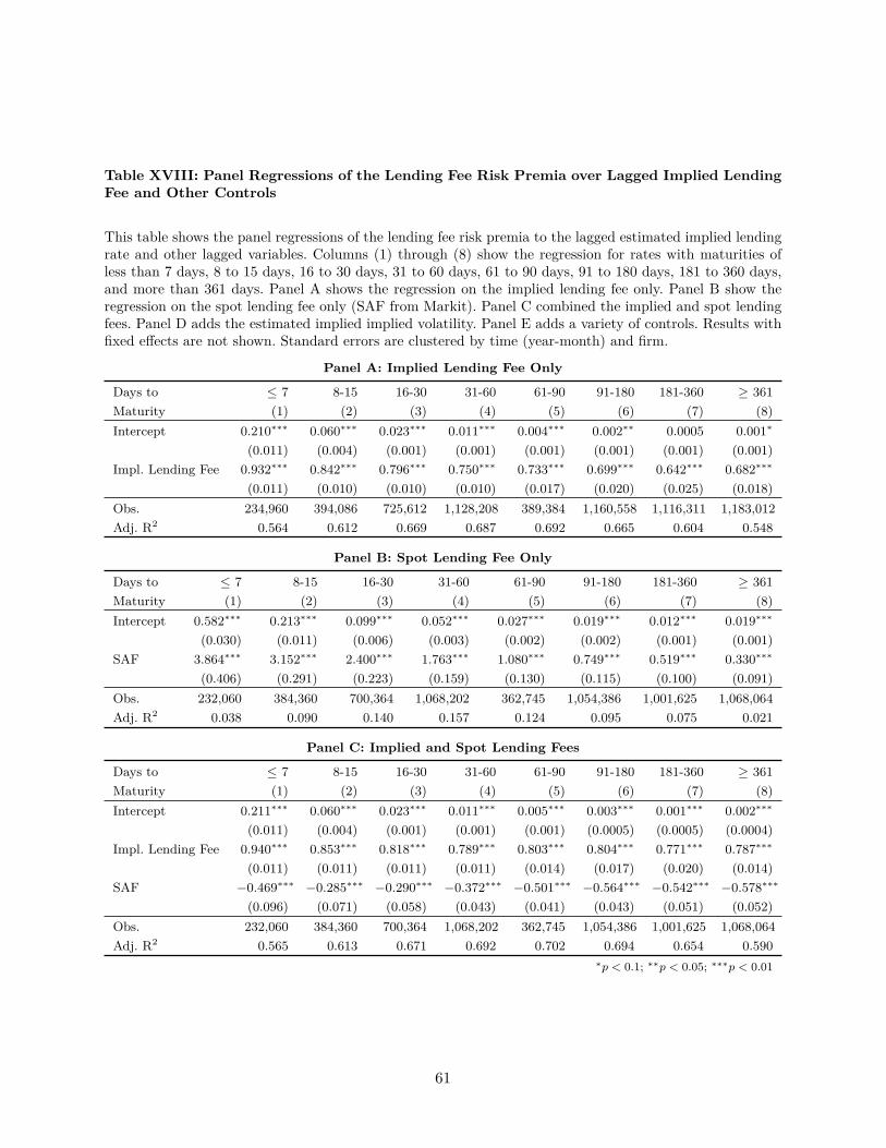
Table XVIII: Panel Regressions of the Lending Fee Risk Premia over Lagged Implied LendingFee and Other Controls

This table shows the panel regressions of the lending fee risk premia to the lagged estimated implied lendingrate and other lagged variables. Columns (1) through (8) show the regression for rates with maturities ofless than 7 days, 8 to 15 days, 16 to 30 days, 31 to 60 days, 61 to 90 days, 91 to 180 days, 181 to 360 days,and more than 361 days. Panel A shows the regression on the implied lending fee only. Panel B show theregression on the spot lending fee only (SAF from Markit). Panel C combined the implied and spot lendingfees. Panel D adds the estimated implied implied volatility. Panel E adds a variety of controls. Results withfixed effects are not shown. Standard errors are clustered by time (year-month) and firm.

Panel A: Implied Lending Fee Only

Days to ≤ 7 8-15 16-30 31-60 61-90 91-180 181-360 ≥ 361Maturity (1) (2) (3) (4) (5) (6) (7) (8)Intercept 0.210∗∗∗ 0.060∗∗∗ 0.023∗∗∗ 0.011∗∗∗ 0.004∗∗∗ 0.002∗∗ 0.0005 0.001∗

(0.011) (0.004) (0.001) (0.001) (0.001) (0.001) (0.001) (0.001)Impl. Lending Fee 0.932∗∗∗ 0.842∗∗∗ 0.796∗∗∗ 0.750∗∗∗ 0.733∗∗∗ 0.699∗∗∗ 0.642∗∗∗ 0.682∗∗∗

(0.011) (0.010) (0.010) (0.010) (0.017) (0.020) (0.025) (0.018)Obs. 234,960 394,086 725,612 1,128,208 389,384 1,160,558 1,116,311 1,183,012Adj. R2 0.564 0.612 0.669 0.687 0.692 0.665 0.604 0.548

Panel B: Spot Lending Fee Only

Days to ≤ 7 8-15 16-30 31-60 61-90 91-180 181-360 ≥ 361Maturity (1) (2) (3) (4) (5) (6) (7) (8)Intercept 0.582∗∗∗ 0.213∗∗∗ 0.099∗∗∗ 0.052∗∗∗ 0.027∗∗∗ 0.019∗∗∗ 0.012∗∗∗ 0.019∗∗∗

(0.030) (0.011) (0.006) (0.003) (0.002) (0.002) (0.001) (0.001)SAF 3.864∗∗∗ 3.152∗∗∗ 2.400∗∗∗ 1.763∗∗∗ 1.080∗∗∗ 0.749∗∗∗ 0.519∗∗∗ 0.330∗∗∗

(0.406) (0.291) (0.223) (0.159) (0.130) (0.115) (0.100) (0.091)Obs. 232,060 384,360 700,364 1,068,202 362,745 1,054,386 1,001,625 1,068,064Adj. R2 0.038 0.090 0.140 0.157 0.124 0.095 0.075 0.021

Panel C: Implied and Spot Lending Fees

Days to ≤ 7 8-15 16-30 31-60 61-90 91-180 181-360 ≥ 361Maturity (1) (2) (3) (4) (5) (6) (7) (8)Intercept 0.211∗∗∗ 0.060∗∗∗ 0.023∗∗∗ 0.011∗∗∗ 0.005∗∗∗ 0.003∗∗∗ 0.001∗∗∗ 0.002∗∗∗

(0.011) (0.004) (0.001) (0.001) (0.001) (0.0005) (0.0005) (0.0004)Impl. Lending Fee 0.940∗∗∗ 0.853∗∗∗ 0.818∗∗∗ 0.789∗∗∗ 0.803∗∗∗ 0.804∗∗∗ 0.771∗∗∗ 0.787∗∗∗

(0.011) (0.011) (0.011) (0.011) (0.014) (0.017) (0.020) (0.014)SAF −0.469∗∗∗ −0.285∗∗∗ −0.290∗∗∗ −0.372∗∗∗ −0.501∗∗∗ −0.564∗∗∗ −0.542∗∗∗ −0.578∗∗∗

(0.096) (0.071) (0.058) (0.043) (0.041) (0.043) (0.051) (0.052)Obs. 232,060 384,360 700,364 1,068,202 362,745 1,054,386 1,001,625 1,068,064Adj. R2 0.565 0.613 0.671 0.692 0.702 0.694 0.654 0.590

∗p < 0.1; ∗∗p < 0.05; ∗∗∗p < 0.01

61

Table XVIII (cont.): Panel Regressions of the Lending Fee Risk Premia over Lagged ImpliedLending Fee and Other Controls

Panel D: Implied and Spot Lending Fees and Implied Volatility

Days to ≤ 7 8-15 16-30 31-60 61-90 91-180 181-360 ≥ 361Maturity (1) (2) (3) (4) (5) (6) (7) (8)Intercept 0.104∗∗∗ −0.010∗∗ −0.015∗∗∗ −0.013∗∗∗ −0.011∗∗∗ −0.007∗∗∗ −0.004∗∗∗ 0.0003

(0.012) (0.004) (0.003) (0.002) (0.002) (0.001) (0.001) (0.002)Impl. Lending Fee 0.870∗∗∗ 0.789∗∗∗ 0.771∗∗∗ 0.749∗∗∗ 0.763∗∗∗ 0.776∗∗∗ 0.752∗∗∗ 0.783∗∗∗

(0.011) (0.013) (0.012) (0.012) (0.016) (0.021) (0.024) (0.015)SAF −0.896∗∗∗ −0.515∗∗∗ −0.380∗∗∗ −0.412∗∗∗ −0.518∗∗∗ −0.573∗∗∗ −0.548∗∗∗ −0.583∗∗∗

(0.083) (0.067) (0.056) (0.041) (0.042) (0.043) (0.051) (0.051)Impl. Vol. 0.358∗∗∗ 0.226∗∗∗ 0.119∗∗∗ 0.071∗∗∗ 0.044∗∗∗ 0.026∗∗∗ 0.016∗∗∗ 0.005

(0.028) (0.017) (0.011) (0.007) (0.005) (0.005) (0.005) (0.005)Obs. 232,060 384,360 700,364 1,068,202 362,745 1,054,386 1,001,625 1,068,064Adj. R2 0.576 0.626 0.680 0.699 0.708 0.697 0.656 0.590

Panel E: All ControlsDays to ≤ 7 8-15 16-30 31-60 61-90 91-180 181-360 ≥ 361Maturity (1) (2) (3) (4) (5) (6) (7) (8)Intercept 2.089∗∗∗ 0.921∗∗∗ 0.316∗∗∗ 0.153∗∗∗ 0.081∗∗∗ 0.045∗∗∗ 0.023∗∗ 0.032∗∗

(0.155) (0.072) (0.033) (0.020) (0.014) (0.011) (0.011) (0.014)Impl. Lending Fee 0.805∗∗∗ 0.748∗∗∗ 0.747∗∗∗ 0.731∗∗∗ 0.751∗∗∗ 0.769∗∗∗ 0.749∗∗∗ 0.787∗∗∗

(0.013) (0.014) (0.013) (0.013) (0.017) (0.023) (0.026) (0.016)SAF −1.036∗∗∗ −0.569∗∗∗ −0.400∗∗∗ −0.396∗∗∗ −0.487∗∗∗ −0.558∗∗∗ −0.530∗∗∗ −0.562∗∗∗

(0.117) (0.071) (0.061) (0.046) (0.048) (0.049) (0.055) (0.052)Impl. Vol. 0.212∗∗∗ 0.150∗∗∗ 0.108∗∗∗ 0.072∗∗∗ 0.047∗∗∗ 0.028∗∗∗ 0.019∗∗∗ 0.004

(0.028) (0.018) (0.011) (0.008) (0.006) (0.006) (0.006) (0.006)RV (20 days) 0.152∗ 0.048∗ −0.033∗∗∗ −0.024∗∗∗ −0.012∗∗ −0.003 0.004 0.015∗∗∗

(0.078) (0.026) (0.010) (0.008) (0.005) (0.004) (0.004) (0.003)Utilization −0.0001 −0.0001 −0.0001 −0.0002∗∗∗ −0.0002∗∗∗ −0.0002∗∗∗ −0.0002∗∗∗ −0.0002∗∗∗

(0.0003) (0.0001) (0.0001) (0.00004) (0.00004) (0.00003) (0.00003) (0.00004)Available Ratio −0.046 −0.101∗∗∗ −0.066∗∗∗ −0.033∗∗∗ −0.016∗∗ −0.007 0.001 −0.001

(0.075) (0.038) (0.018) (0.010) (0.007) (0.005) (0.004) (0.005)Log(Var(SAF)) −0.005∗∗∗ −0.001 −0.0003 −0.0002 −0.0003∗∗ −0.0002∗∗∗ −0.0002∗∗∗ −0.0004∗∗∗

(0.001) (0.001) (0.0004) (0.0002) (0.0001) (0.0001) (0.0001) (0.0001)Log(Var(Util.)) −0.012∗∗∗ −0.009∗∗∗ −0.004∗∗∗ −0.002∗∗∗ −0.001∗∗∗ −0.0002 0.0004 0.001∗∗

(0.002) (0.001) (0.001) (0.0004) (0.0003) (0.0002) (0.0002) (0.0003)Avg. Tenure 0.0003∗∗∗ 0.0001∗∗∗ 0.0001∗∗∗ 0.00003∗∗∗ 0.00002∗∗∗ 0.00001∗∗∗ 0.00001∗ 0.00001∗∗

(0.0001) (0.00003) (0.00002) (0.00001) (0.00000) (0.00000) (0.00000) (0.00000)Inv. Concentr. 0.224∗∗ 0.098∗∗ 0.070∗∗∗ 0.049∗∗∗ 0.023∗∗∗ 0.011∗ 0.006 0.004

(0.102) (0.049) (0.022) (0.014) (0.007) (0.006) (0.007) (0.008)Loan Concentr. 0.028 0.002 0.001 −0.001 −0.0002 0.0003 0.001 0.002

(0.021) (0.009) (0.004) (0.003) (0.002) (0.001) (0.001) (0.001)Demand Concentr. −0.006 −0.001 −0.004 −0.003 −0.002 −0.0004 −0.0004 −0.001

(0.020) (0.009) (0.005) (0.003) (0.002) (0.001) (0.001) (0.001)Log(Mkt. Cap.) −0.086∗∗∗ −0.038∗∗∗ −0.013∗∗∗ −0.007∗∗∗ −0.004∗∗∗ −0.002∗∗∗ −0.001∗∗∗ −0.002∗∗∗

(0.006) (0.003) (0.001) (0.001) (0.001) (0.0005) (0.0004) (0.0005)Obs. 224,171 370,754 675,323 1,030,188 349,831 1,018,025 967,368 1,037,432Adj. R2 0.592 0.635 0.682 0.697 0.709 0.696 0.655 0.592

∗p < 0.1; ∗∗p < 0.05; ∗∗∗p < 0.0162

the term structure of securities lending...

Documents