i

The Thesis Committee for Jacob R. Smith

Certifies that this is the approved version of the following thesis:

A Comparison of Reservoir Gas Energy and Composition with

Respect to Initial Oil Production in the San Andres Formation of

Shafter Lake Field, Andrews County, Texas.

APPROVED BY

SUPERVISING COMMITTEE:

John S. Wickham

John E. Damuth

William J. Moulton

ii

A COMPARISON OF RESERVOIR GAS ENERGY AND COMPOSITION

WITH RESPECT TO INITIAL OIL PRODUCTION IN THE SAN ANDRES

FORMATION OF ANDREWS COUNTY, TEXAS.

BY

Jacob R. Smith

Thesis Presented to the Faculty of the Graduate School of

The University of Texas at Arlington

in Partial Fulfillment

of the Requirements

for the Degree of

Master of Science in Petroleum Geoscience

The University of Texas at Arlington

May 2018

iii

ABSTRACT

The oil-rich, Permian-age San Andres Formation in the Permian Basin of West Texas

produces Wolfcampian-age oil from the dolomitic host rock in prolific amounts. The present

study focuses on the Shafter Lake field and utilizes gas analysis reports, well parameters,

and 24-hour initial production (IP) reports of oil and associated petroleum gases

(preferential to methane) to determine if a correlation exists between formation gas and oil

production in the San Andres formation. The San Andres formation undergoes a substantial

de-watering process before peak oil-production commences, and this study briefly touches

on that subject to account for the massive initial water production which far exceeds the IP

of oil. Since the horizontal wells have a first and last perforated zone differential of, on

average, twenty-eight times the directional wells, the data is normalized by dividing the

production by linear feet of perforated zones. With well type accounted for, normalized IP

of oil cross-plotted against normalized IP of gas shows a correlation coefficient of 0.906,

which is just over a 90% relation between the oil produced and formation gas produced

with it. This relationship can be inferred as either higher oil mobility caused by either gas-

cut saturation, or an expanding gas-cap drive upon de-pressuring of the reservoir as a result

of extensive production.

iv

Table of Contents

List of Figures………………………………………………………………………………………………………………………vi

Introduction…………………………………………………………………………………………………………………………1

Background and Geologic Setting…………………………………………………………………………………………2

Permian Basin………………………………………………………………………………………………………..2

Tectonic History of the Permian Basin……………………………………………………………………6

The San Andres Formation…………………………………………………………………………………….7

Drilling Hazards Associated with the San Andres Formation………………………….……..11

Objectives of Study and Expected Outcomes………………………………………………………………..……12

Location of Study………………………………………………………………………………………………………………..13

Effects of Gas in Solution on Oil Viscosity…………………………………………………………………………...19

Research Design and Procedures………………………………………………………………………………………..21

Data and Methods……………………………………………………………………………………………………….……..22

Production and Wellbore Data……………………………………………………………………………..22

Gas Analysis………………………………………………………………………………………………………….23

Results and Discussion………………………………………………………………………………………………………..25

v

Results………………………………………………………………………………………………………………………………..56

Conclusion………………………………………………………………………………………………………………………….58

References………………………………………………………………………………………………………………………….59

vi

List of Figures

FIGURE 1: PALEOGEOGRAPHIC TIME-SEQUENCE OF THE GREATER PERMIAN BASIN 3

FIGURE 2: PALEOGEOGRAPHIC MAP OF THE PERMIAN BASIN DURING THE PERMIAN 4

FIGURE 3: BASINS, PLATFORMS, AND OUACHITA-MARATHON THRUST BELT IN THE PERMIAN BASIN 5

FIGURE 4: PHYSIOGRAPHIC DIAGRAM DEPICTING THE PERMIAN BASIN WITH FORMATION TABLE 9

FIGURE 5: ILLUSTRATION DEPICTING A HORIZONTAL AND DIRECTIONAL WELLBORE 14

FIGURE 6: LOCATION OF THE STUDY AREA WITHIN THE CENTRAL BASIN PLATFORM 15

FIGURE 7: REGIONAL MAP OF RESERVOIRS THAT HAVE PRODUCED MORE THAN 1 MILLION BBL OIL 16

FIGURE 8: BLOCKS 13 AND 14 IN NORTHERN ANDREWS COUNTY MARKING STUDY AREA 17

FIGURE 9: BLOCKS 13 AND 14 ENLARGED WITH OIL WELLS AND WELLBORES DEPICTED 18

FIGURE 10: SOLUTION GAS-OIL RATIO AND EFFECTS ON BUBBLE POINT IN A RESERVOIR 20

FIGURE 11: MOLE PERCENTAGES OF NATURAL GAS LEVELS IN THE SAN ANDRES FORMATION 24

FIGURE 12: INITIAL PRODUCTION OF OIL CONTOUR MAP 27

FIGURE 13: INITIAL PRODUCTION OF GAS CONTOUR MAP 28

FIGURE 14: INITIAL PRODUCTION OF WATER CONTOUR MAP 29

FIGURE 15: NORMALIZED INITIAL PRODUCTION OF OIL CONTOUR MAP 31

vii

FIGURE 16: NORMALIZED INITIAL PRODUCTION OF GAS CONTOUR MAP 32

FIGURE 17: NORMALIZED INITIAL PRODUCTION OF WATER CONTOUR MAP 33

FIGURE 18: STACKED BAR GRAPH OF NORMALIZED OIL + WATER (RAW) 34

FIGURE 19: STACKED BAR GRAPH OF NORMALIZED OIL + WATER 35

FIGURE 20: CROSS PLOT OF IP OIL (BBL) COMPARED TO IP GAS (MCF) 37

FIGURE 21: CROSS PLOT OF IP OIL + WATER (BBL) COMPARED TO IP GAS (MCF) 38

FIGURE 22: CROSS PLOT OF IP OIL (BBL) COMPARED TO WELLBORE DEPTH (TVD) (FT) 40

FIGURE 23: CROSS PLOT OF IP WATER (BBL) COMPARED TO WELLBORE DEPTH (TVD) (FT) 41

FIGURE 24: CROSS PLOT OF NORMALIZED IP OIL (BBL) COMPARED TO WELLBORE DEPTH (TVD) (FT) 43

FIGURE 25: CROSS PLOT OF PERFORATED ZONE (FT) COMPARED TO IP OIL (BBL) 44

FIGURE 26: CROSS PLOT OF NORMALIZED IP OIL (BBL/FT) COMPARED TO PERFED ZONE DIFFERENTIAL (FT) 46

FIGURE 27: SCATTER PLOT OF TVD (FT) OF HORIZONTAL AND DIRECTIONAL WELLS 47

FIGURE 28: NORMALIZED IP OF OIL COMPARED TO NORMALIZED IP OF GAS 50

FIGURE 29: CROSS-PLOT OF IP OIL VS IP GAS OF DIRECTIONAL WELLS (NORMALIZED) 51

FIGURE 30: CROSS-PLOT OF IP OIL VS IP GAS OF HORIZONTAL WELLS (NORMALIZED) 52

viii

FIGURE 31: CONTOUR MAP OF THE GAS-OIL RATIO (GOR) DISTRIBUTION IN ALL WELLS 54

FIGURE 32: CONTOUR MAP OF THE OIL-CUT DISTRIBUTION IN ALL WELLS 55

1

INTRODUCTION

The Permian aged San Andres Formation in West Texas is both a conduit and a

reservoir for hydrocarbons; however, the various fields do not maintain uniform

normalized production of hydrocarbons. Old water floods, carbonate ramp

compartmentalization, (Ramondetta 1982) and H2S gas from sulfate-reducing bacteria

make this formation highly variable in terms of its oil production rate. The methane-gas

drive in the reservoir is probably the primary control on the normalized production

rate. When portions of the hydrocarbons derived from Wolfcampian basinal clastics

and dark argillaceous limestones mature and move from the oil window to the gas

window, the oil loses density and gains energy (Ramondetta 1982). Methane is

dissolved into the remaining oil making the oil more mobile. In theory, the oil will then

flow more easily from host rock through the production liner or casing. Consequently,

as the play is produced and the reservoir pressure drops below the bubble point, the

methane comes out of solution and expands to create the methane gas drive. The gas

cap increases and the oil “shrinks” as gas is liberated from the solution. This natural-gas

drive can provide enough pressure for oil to reach the surface before the use of an

artificial gas lift, neighboring injection well, or pumping unit is installed at the wellhead.

The purpose of this study is to determine if a correlation exists between methane gas

levels and initial production of the well by studying sixty-two wells in the Shafter Lake

Field of the San Andres Formation.

2

BACKGROUND AND GEOLOGIC SETTING

Permian Basin

The Permian Basin is one of the largest structural basins in North America (~86,000 sq.

mi.) and covers 52 counties throughout West Texas and Southeast New Mexico (Ball,

1995). This vast, oil-rich desert is composed of the Midland Basin on the east, Delaware

Basin to the west. The Central Basin Platform, which is a northwest-southeast trending

basement uplift, separates the two basins (Figures 1 and 2). The significantly deeper

Delaware Basin is a thicker, more structurally deformed sequence of sedimentary rocks

than the Midland Basin, which is thinner and higher in the section. However, the

Midland Basin contains many of the same sedimentary deposits as the Delaware Basin,

and the Central Basin Platform. The Permian Basin today is, for the most part,

unchanged since the Early Permian. The Paleozoic sediments are overlain by a

relatively thin succession of Mesozoic and Cenozoic sedimentary strata. Oil and gas

have been found in rocks as old as the Cambrian, and as young as the Cretaceous, but

the Paleozoic rocks dominate production (Ball, 1995). The Permian Basin is bounded on

the north by the Matador Arch, the east by the Eastern Shelf of the Midland Basin, the

south by the Ouachita-Marathon Fold-Thrust Belt, and on the west by the Diablo

Platform (Figures 2 and 3). A broad understanding of the Permian Basin’s complex

development through geologic time is pertinent to understanding its small-scale

geology.

3

Figure 1. Paleogeographic time-sequence of the greater Permian Basin. (Sutton, 2014). State boundaries and labels in red, Permian Basin area encircled in red.

4

Figure 2. Central Basin Platform (CBP), Delaware (DeB), and Midland (MiB) basins taking shape within the Tobosa Basin during the Permian (Blakely, 2013). Once the northwest trending CBP was uplifted, the Tobosa ceased to exist and the one basin became two.

5

Figure 3. The basins, platforms, and thrust belt that comprise the modern-day Permian Basin. (Encyclopedia Britannica, 2007)

6

Tectonic History

During Paleozoic time, the modern-day Permian Basin was the Tobosa Basin, which

contained a shallow, vast, and continuous intracratonic sea. The modern Central Basin

Platform, which is an uplifted zone of basement rock formed during middle-to-late

Pennsylvanian (Figure 1, middle image, Figure 2) (Hoak et al, 1998). During the

formation of Pangea in the middle-to-late Paleozoic, Laurasia and Gondwana collided,

forming the Ouachita-Marathon thrust belt (Figures 2 and 3) and a related foreland

basin. The Midland and Delaware basins, along with a small number of less extensive

sub-basins formed from the Mississippian to early-mid Permian time in the foreland

basin of the Ouachita thrust belt (Hoak et al, 1998) (Figure 3).

During the Late Paleozoic glacial period, rapid basin subsidence combined with glacio-

eustatic sea level changes, along with the proximal uplift of the Central Basin Platform,

allowed sediments to accumulate in the newly formed Midland and Delaware basins

(Ramondetta 1982). With the production of this new accommodation space, basinal

clastics were deposited during the Wolfcampian and Leonardian in rapid succession.

The bulk of these deposits were calcareous and siliceous mudrocks, as well as skeletal

packstones and grainstones. These interbedded shales and argillaceous limestones are

widely considered to be the source rocks for the oil that migrated to the San Andres

Formation (Ramondetta 1982).

7

The San Andres Formation

The San Andres Formation in the Central Basin Platform and the Midland Basin was

deposited during the Guadalupe Epoch of the Permian (Figure 4). From currently

producing vertical wells drilled in the 1920’s, to 2-mile multi-staged, acidized, fractured

laterals completed in 2017, the amount of oil in place in the top 4 major Permian Basin

oil plays in the San Andres Formation is estimated at 28.1 billion barrels of oil in place

(BBOIP) for only main pay zones (Melzer et al. 2011). These 4 zones are the Northern

Shelf, north Central Basin Platform, south Central Basin Platform, and east New

Mexico. According to Melzer et al. (2011), the transitional zones and residual oil zones

contain an estimated 27.8 billion barrels of oil in place. Based on reservoir modeling,

Advanced Resources International, Inc. (2011) estimates that 10.6 billion barrels of oil

(BBO) are technically recoverable from these top four Permian Basin oil plays in the San

Andres using secondary/tertiary recovery methods including but not limited to CO2

flooding. Dutton et al. (2005) estimated that 75% of total oil production in the Permian

Basin is produced from carbonate reservoirs; however, these data were published

before the horizontal shale boom in the Permian.

8

Of the more than 30 billion barrels of oil (BBO) produced from the Permian Basin,

approximately 40% or 12 BBO and 2 trillion cubic feet (Tcf) of gas came from the San

Andres Formation (Ring Energy, 2018). This “conventional shallow non-contiguous

carbonate reservoir” is approximately 5,000’ deep in the Central Basin Platform, and

produces about 95% oil (Ring Energy, 2018). Many private equity-funded operators are

drilling long laterals in the shallow San Andres, which produce more economically than

the older style conventional vertical wells. Compared to a much deeper horizontal

Bone Springs/Spraberry/Wolfcamp (Figure 4) mudrock well, these operators are saving

millions of dollars. Because the San Andres is nearly a mile higher in section, the

operators drilling horizontal wells in the San Andres are utilizing the smaller, less

expensive drilling rigs that have a much lower demand than the larger rigs used for

Wolfcamp/Spraberry/Bone Springs targets. According to an investor presentation from

Ring Energy in 2018, their average well cost for a Central Basin Platform San Andres

(CBP SA) well is $2MM for a 1 mile lateral and 2.4MM for a 1.5 mile lateral. Conversely,

according to an unnamed company drilling primarily Wolfcamp wells in the Delaware

Basin, a 6,000 foot lateral costs an average of $6.8MM to complete. Because of this

huge differential, combined with the advancement of multi-stage fracking, and acid-

fracking technology, producing from dolomitic host rock is becoming much more

economical than previously.

9

Figure 4. Physiographic diagram depicting the Permian Basin. Tables show the Permian formations present. (Warren 2014).

10

The San Andres Formation is a dolomitized, shallow-water, carbonate platform facies

which is exclusive to the Northwestern Shelf, Central Basin Platform, the Eastern Shelf

of Midland Basin, and the Ozona Arch. Silicate sands also occur in the San Andres

Formation, along with these mostly dolomitized carbonates and probably represent

deposition in response to sea-level fluctuations. Another characteristic of this

dolomitized carbonate play is the evaporitic seals of anhydrite and gypsum, which

formed as the sea evaporated, and act as impermeable reservoir seals. Prolific amounts

of oil and gas occur in the platform sequence of carbonate and fine-grained silicate

reservoirs, which formed stratigraphic and structural traps in the dolomitic host rock

(Ramondetta 1982).

The carbonate rocks comprising the San Andres Formation were deposited on open-to-

restricted platforms and platform margins. Eustatic sea-level fluctuations in the

Paleozoic influenced shelf-margin reef development, and sabkhas, which formed the

evaporitic seals. Whereas dolomitized carbonate rocks dominate the lithology of the

San Andres, skeletal grainstones, limestones, calcareous and silty sandstones, sponge

and algal dolomitized limestones, dolomitized mudstones and wackestones, and vuggy

to cavernous carbonate beds can all be found in the play (Ball 1995).

Although the San Andres is primarily tapped for its large oil reserves, gas is readily

available for production. After the San Andres Mountain uplift in southwestern New

Mexico during the late Oligocene and early Miocene (Melzer et al, 2011) (Ramondetta

1982) meteoric waters infiltrated the karsted San Andres outcrop and allowed the

formation to undergo a great water flooding event. This water flood was instrumental in

11

the formation of the water-charged San Andres aquifer, residual oil zones, and

transitional zones.

Drilling Hazards Associated with the San Andres Formation

The San Andres Formation is well known as a problem reservoir in terms of its

variability in production and associated drilling hazards. One of the hazards associated

with the drilling phase is high permeability and even cavernous sections where lost

circulation of drilling fluids is very common and costly for the operating company.

Many areas of the San Andres Formation are partially or fully depleted, meaning the

reservoir pressure is too low to support the weight of the drilling mud column, which

causes the mud to inundate the porous carbonate formation that can have as much as

20% matrix porosity. Reservoir pressure depletion is caused mainly by the extensive

production of this formation spanning over 70 years. Companies losing thousands of

barrels a day of costly drilling mud have been known to pump lost circulation material

(LCM) as large as golf balls in an attempt to plug the cavernous porosity encountered.

Other types of LCM pumped downhole include cedar wood fiber, walnut hulls,

cottonseed hulls, or micaceous material. If the formation is taking in all or most of the

drilling fluids, there is no mud column keeping pressures controlled and the well can

experience a kick of high-pressure gas, which can be devastating to the rig personnel

and equipment. Another problem of losing the mud column is differential sticking of

12

the drill string to the side slurry of dehydrated mud cake which sets and holds the drill

pipe in place with the help of a differential pressure in the zone (Wiley, 1998).

Yet another of these hazards is the characteristically high concentration of hydrogen

sulfide gas or H2S, which is a poisonous gas that is deadly to humans in even small

concentrations. H2S can be highly corrosive to the drill string and BHA. Many operators

use the San Andres formation as a marker for setting their intermediate casing because

of all the associated problems when drilling through it in order to reach a target

formation lower in section. Casing through this formation saves mud loss, suppresses

H2S gas, and keeps water floods and kicks from disrupting operations.

OBJECTIVES OF THE PRESENT STUDY

As fluid migration began in the San Andres Formation, stratigraphic pinch-outs created

compartmentalized reservoirs, which contain variable amounts of trapped

hydrocarbons (Rodriguez and Gong, 2017). With this variation in volatile hydrocarbons

throughout the San Andres, it is my hypothesis that regions with the higher

concentration of methane and thus, gas energy, will experience greater oil

mobilization, and a higher initial production rate, assuming all other things affecting

production are equal. Therefore, the objective of this study is to determine if a

correlation exists between the methane gas levels and initial oil production.

13

LOCATION OF STUDY

The study area is the Shafter Lake Field located in northern Andrews County, Texas, 36

miles southeast of the Northwest Shelf and 16 miles west of the Midland Basin (Figures

6 and 7). The specific study area within the Shafter Lake field is Blocks 13 and 14, which

is comprised of vertical, directional, and horizontal wells of the University Lands oil and

gas easements (Figures 8 and 9). These two blocks are roughly 75 sq. miles or 193 sq.

kilometers in size. The University Lands organization provides free, public drilling and

completions data and is the majority of the data used in this thesis. This study will

exclusively use only the directional and horizontal wells in these 2 blocks. This is done

to minimize outliers based on the old technologies of the vertical wells drilled as early

as the 1920’s. In contrast, the average date of drilling/completion of the directional and

horizontal wells is 2014. The term “directional well” in this study refers to a wellbore

intentionally deviated to target potential reservoirs at a specific location more

effectively. The deviated wellbores are not horizontal wells, and are typically much

shorter in horizontal displacement form the surface location. Figure 5 contains an

illustration depicting horizontal and directional wellbores. The vertical wells are also

left out of the study data for the simple fact that operating companies are far less likely

to drill a straight vertical well in this age of advanced directional technologies.

14

Figure 5. Illustration depicting the differences between a horizontal (left) and a directional (right) wellbore. The image is not to scale, and acts as a simple sketch to demonstrate different drilling techniques discussed in this paper.

15

Figure 6. The solid red circle indicates the location of study area within the Central Basin Platform. (Image modified from the University Lands Well Data App)

16

Figure 7. Central Basin Platform San Andres fields in the Permian Basin that have produced more than 1 million barrels of oil. The Shafter Lake Field is shown in red. (Modified after Dutton et. al., 2005)

17

Figure 8. Blocks 13 and 14 of the Shafter Lake Field within the blue circle in northern Andrews County. (Image modified from the University Lands Well Data App).

18

Figure 9. Blocks 13 and 14 showing locations of horizontal and directional oil wells (green circles for surface location, small blue circles for bottom-hole location). Wellbore locations included, and area covers all sixty-two wells in the study area. (Image from the University Lands Well Data App with Petra overlay). The directional wells in this study are located in sections 16, 17, and 18 of Block 14; and in section 37 of Block 13.

19

EFFECTS OF GAS IN SOLUTION ON OIL VISCOSITY

The bubble point is defined as the state at which an infinitesimal quantity of gas is in

equilibrium with a large quantity of liquid (Dandekar 2013). The liquid in this case is

crude oil and the gas is primarily methane. Because the reservoir pressure is above the

bubble point, the oil is able to retain more gas in solution until the reservoir pressure

drops below the bubble point and the gas is liberated from solution (Figure 10). Before

a reservoir is produced, this crude oil will be saturated with associated petroleum

gases. As production initiates de-pressuring of the reservoir, free gas will be liberated

from solution and affects the mobility of the oil. As a reservoir’s pressure drops, gas is

liberated, the gas cap expands, and this cap can provide additional drive energy (Figure

10). The relative permeability of the host lithology will have a greater effect on

movement of oil and gas, but the bubble point plays an important role. In recovering

under-saturated oil, volumetric changes in oil and gas above the bubble point are

prodigious. This effects the oil compressibility and consequently, how much reserves

are in the host rock.

20

Figure 10. Solution gas-oil ratio and the effects of the bubble point on saturation of natural gas in a reservoir (Dandekar, 2013).

21

RESEARCH DESIGN AND PROCEDURES

Initially, contour maps illustrating the geographical location of the Shafter Lake wells,

and the 24-hour initial production data of said wells were produced. These public data

are available through the University Lands website. Petra software was then utilized to

create contour maps of IP oil, IP gas, and TVD contours of lateral wellbores using

location of wellbores defined by longitude and latitude. Cross plots of the numerical

production data were produced to supplement the visual comparisons between the

aforementioned data. Cross plots of this production data versus various wellbore

locations/lengths/producing intervals demonstrate the correlation between the data.

Inferred formation dip, true vertical depth, and well data, were used to distinguish

different units within the San Andres play in the Shafter Lake Field and group them

together. Once grouped, a series of cross plots of oil vs. gas with different control

factors are used to determine which unit has the best production/drive.

22

DATA AND METHODS

Production and Wellbore Data

In order to complete the research for this study, initial production data, perforated

zones and wellbore location, true vertical depth, and latitude and longitude were used.

These data were provided by operating companies to the University Lands System,

comprised of the Texas A&M University System in conjunction with the University of

Texas System and the Bureau of Economic Geology. The primary research control in

this study was demonstrated by contour maps and Z-cross plots of different IP data and

where and how the well was drilled. Comparisons and normalizations of the perforated

intervals were used to further constrain the controls of the research. Directional and

horizontal wells differ in length of perforated zones by as much as 10,035’ in the most

extreme case in this study. To account for this wide variation in productive intervals,

the production is normalized to perforated zone differential. As exact perforation

clusters, shot charges and fracking operations are typically kept confidential, this study

implements the differential of the fist perforation and the last perforation, and

assumes similar completion practices.

23

Gas Analysis

Chromatograph analysis of associated petroleum gases were provided for the present

study by an anonymous operator. Consequently, the exact location and number of

wells sampled remains confidential. These gas analysis reports took molar percentage

measurements of natural gases produced from Shafter Lake wells to the ten-

thousandth place. The average of these percentages was utilized to gain an estimate of

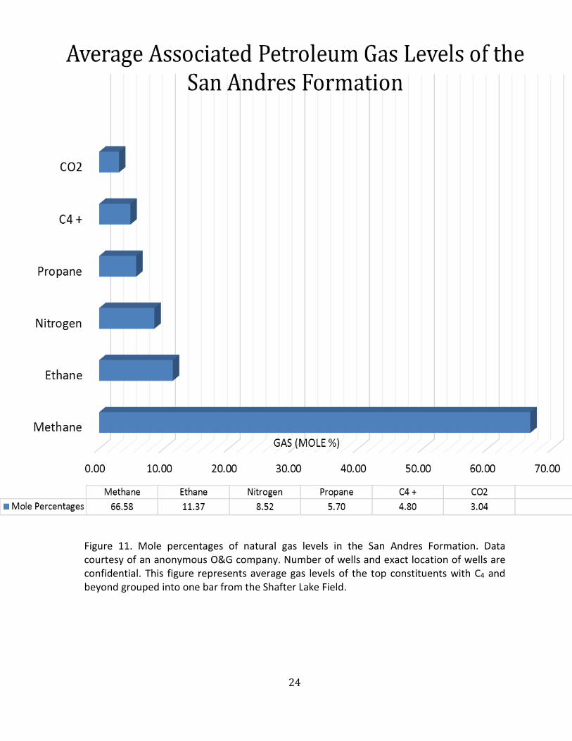
the gases in the formation that are available to initiate gas drive. Figure 11 shows that

Methane (CH4) is the main constituent of associated petroleum gas in the Shafter Lake

field at 66.58%, followed by Ethane (C2H6) at 11.37%, Nitrogen (N2) at 8.52%, Propane

(C3H8) at 5.70%, Carbon Dioxide (CO2) at 3.04%, and C4+ at a combined 4.80%. Before

the averaging, this data is equitably consistent with each sampled well in terms of

ratios of the natural gas concentration, and therefore, for the purposes of this study,

have been considered equal in all the wells in the study area. The chromatograph

analysis of several of these wells puts the highest constituent of associated petroleum

gas at methane, and as a result, when the word “gas” is used, the term is preferential

to methane.

24

Figure 11. Mole percentages of natural gas levels in the San Andres Formation. Data courtesy of an anonymous O&G company. Number of wells and exact location of wells are confidential. This figure represents average gas levels of the top constituents with C4 and beyond grouped into one bar from the Shafter Lake Field.

25

RESULTS AND DISCUSSION

Using Petra software, contour maps were created based on the initial production of all

sixty-two wells in the study area. Figure 12 shows the Shafter Lake field with IP in barrels

of oil produced in contour map form. This map is not yet normalized, and shows the raw

data before perforated zones were taken into account. The north-east quadrant in the

mapped area experienced the lowest initial oil production, and had the highest

concentration of wells. These wells are almost exclusively directional wells with shorter

relative productive zone than the longer horizontals. There appears to be a northwest-

southeast trending region with the highest raw initial oil production.

Figure 13 represents the initial production of gas. The IP oil map (Figure 12) and the IP

gas map (Figure 13) share many characteristics in terms of raw production distribution.

This map has not been normalized and should be treated as raw data. The north-east

quadrant of both maps is dominated by low production, but this is because it is made

almost entirely of directional wells with shorter perforated intervals. The regions with

the highest oil production are the same regions which experienced the highest gas

production. This visual trend is a potential indicator of areas that can expect to

experience higher levels of initial production.

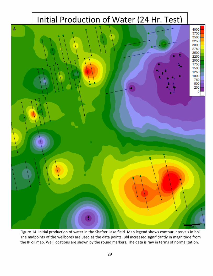
A non-normalized map of the initial water production is shown in Figure 14. The San

Andres Formation experienced massive water floods. Consequently, a dewatering phase

is necessary for this formation to de-pressure and allow the gas to come out of solution

for the gas drive. The IP oil map has a maximum 700 bbl; whereas the IP water map has

26

3,450 bbl. Figure 15 shows the true extent of water this formation produces in its early

stages. The initial water production far outweighs the initial oil production.

27

Figure 12. Initial production of oil in the Shafter Lake field. Map legend shows contour intervals in bbl. The midpoint of the wellbores is used as the data point. Green markers show oil well surface-hole locations with black lines outlining wellbore location. This data is not normalized.

Initial Production of Oil (24 Hr. Test)

28

Figure 13. Initial production of gas in the Shafter Lake field. Map legend shows contour intervals in mcf. The midpoint of the wellbores is used as the data point. Well locations shown by larger green/black markers with black lines tracing wellbores. This data has not been normalized.

Initial Production of Gas (24 Hr. Test)

29

Figure 14. Initial production of water in the Shafter Lake field. Map legend shows contour intervals in bbl. The midpoints of the wellbores are used as the data points. Bbl increased significantly in magnitude from the IP oil map. Well locations are shown by the round markers. The data is raw in terms of normalization.

Initial Production of Water (24 Hr. Test)

30

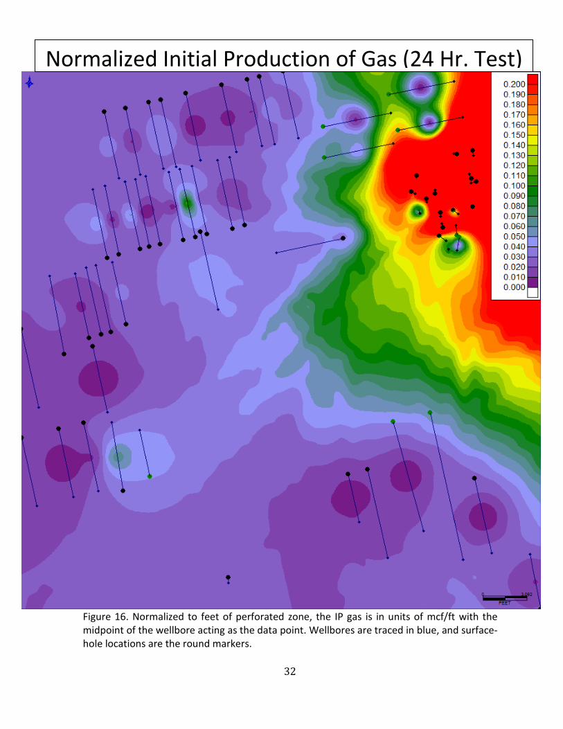
Upon normalizing the oil, gas, and water IP data, the high magnitude areas have

concentrated in the northeast quadrant. This area is made of almost exclusively the shorter

directional wells. Based on figure 15 and figure 16, one can expect the northeast section to

be the prime drill location, but this isn’t necessarily the case. The directional wells seem to

outperform the horizontal wells in barrels of oil and thousand cubic feet of gas per foot, but

wellbore length is crucial to understanding the system as a whole. The directional also seem

to have produced a higher water value per foot as well (Figure 17). Yes, the horizontal wells

have a lower normalized rate, by a significant factor, but the raw data (Figure 12 and 13)

show the magnitude of oil actually produced by the longer laterals.

A stacked-bar graph is used to show the raw data for liquids produced (Figure 18) with oil

and water differentiated. The graph also has wellbore types grouped together to show how

the well design affects IP. Figure 18 shows the horizontal wells far exceeding the directional

in total liquids produced, but a considerable portion of each wells production is formation

water. Disposing of large amounts of connate water is expensive and it takes up valuable

room in stock tanks. Operators try to avoid producing water because it has no value, and

costs them money to have tankers haul it away and dispose of it in salt water disposal wells

(SWD) which also costs money. A normalized stacked-bar graph (Figure 19) shows the

trends swapped in the favor of the directional wells. As previously discussed, the directional

normalized production of all fluids (oil, gas, water) outweighs the horizontals in amount per

foot of perforated length.

31

Figure 15. IP oil is normalized to perforated interval showing units in bbl/ft of oil. The midpoint of the wellbores is used as the data point. The directional wells in the northeast corner are showing higher normalized IP values.

Normalized Initial Production of Oil (24 Hr. Test)

32

Figure 16. Normalized to feet of perforated zone, the IP gas is in units of mcf/ft with the midpoint of the wellbore acting as the data point. Wellbores are traced in blue, and surface-hole locations are the round markers.

Normalized Initial Production of Gas (24 Hr. Test)

33

Figure 17. Normalized to feet of perforated zone, the IP of water shows a bias towards the directional wells in the northeast corner. Contour units are in bbl/ft. The midpoint of the wellbores are used as the data points.

Normalized Initial Production of Water (24 Hr. Test)

34

Figure 18. This stacked bar graph shows the extent of the initial water production of the San Andres Formation in its early stages. The full bar height is the total liquid production during the 24-hour testing interval - oil (red) and water (blue). This data is raw, and has not been normalized.

35

Figure 19. This normalized stacked bar graph shows the extent of the initial water production of the San Andres Formation in its early stages. The full bar height is the total liquid production during the 24-hour testing interval - oil (red) and water (blue). This data has been normalized to linear feet of the perforated zone to show (bbl/ft).

36

The Initial production of gas, preferential to methane, cross-plotted against the initial

production of oil has a correlation coefficient (R) of .564 for a best-fit linear trend line

(Figure 20). There are obvious outliers, which are to be expected. The arduous and

classically inaccurate barrel of oil equivalent (BOE) calculations for this graph are

omitted and the standard mcf and bbl units are used in the entirety of this thesis. As

barrels of oil is compared to thousand cubic feet of gas, the correlation coefficient

equaling 1.00 would not necessarily mean that they are 1:1 correlated. Different units of

different matter cannot be compared directly with zero error, and the trend line and R

value in Figure 20 shows they are, indeed, correlated to some degree; however, we

cannot give too much credence to a value so low on an un-normalized plot. This visual

aid demonstrates that there is some correlation between the amount of associated

petroleum gas and the amount of produced oil in the reservoir of study.

IP of gas in mcf versus IP of (oil + water) in bbl is represented in Figure 21. The shorter

wellbores of the nineteen directional wells are clustered at the bottom of the graph,

with oil + water production totaling under 1,000 bbl for the 24-hour testing period.

Because a smaller correlation coefficient of .362 is observed in Figure 21, the data

seems less conclusive than in Figure 20. However, the trend line is still trending in a

positive direction, showing that there is some relation between the amount of gas in the

reservoir and how much liquid is being produced. Water has a higher density than oil,

which makes it harder to get to the surface than the average barrel of oil.

37

Figure 20. Plot of IP Gas (mcf) on the vertical axis compared to IP Oil (bbl) on the horizontal axis from 62 wells in the study area shows a positive slope with a correlation coefficient of .564. As more oil was produced, the produced gas levels from the reservoir went higher.

38

Figure 21. Plot of IP Oil + IP Water (bbl) on the vertical axis compared to IP Gas (mcf) on the horizontal axis from 62 wells in the study area shows a positive slope with a correlation coefficient of .362.

39

Initial production of oil compared to wellbore depth in true vertical depth (ft) (Figure 22)

shows a strong correlation between how deep the well was drilled and the amount of

produced oil. The wells drilled higher in section are producing vastly larger amounts of oil.

However, the data are un-normalized to the perforated interval. These data are raw, so the

correlation appears strong. Based on knowledge of how a petroleum system works, the

data shown in Figure 22 fits the profile of the lighter hydrocarbons resting on top of the

higher density water. If this relationship holds true, Figure 23 should show a negatively

trending correlation line, showing the deeper the well, the more water produced. However,

this is not the case as the trend line still shows a positive inclination. This plot shows the

shallower the well, the more water is produced. This contradicts our standard petroleum

system interpretation. In this plot (Figure 23) there is a clustered line of data points which

consist of the deepest wells with the lowest water production. This could be the cluster of

the shorter directional wells that is throwing off the data set. In order to account for this,

the top and bottom perforated zone differential is used to normalize production to linear

feet of perforated zone. In theory, dividing production by the perforated differential should

give us bbl of mcf per foot, which will normalize the production rates in an effort to reduce

error between different wellbore types.

40

Figure 22. Initial oil production (bbl) compared to wellbore depth in true vertical depth (ft). This plot shows raw data, un-normalized to perforated zone. These data show that the deeper wells produced less oil than the wells higher in section. This plot is a pseudo-cross-section into the San Andres Formation.

41

Figure 23. Initial water production (bbl) compared to wellbore depth in true vertical depth (ft). This plot is raw data, un-normalized to the perforated zone. These data shows the deeper wells produced less water than the wells higher in section. This plot is a pseudo-cross-section into the San Andres Formation. Notice the X-axis scale change in magnitude due to high-water content of the San Andres Formation.

42

Figure 24 shows the normalized initial production of oil per linear foot of the perforated

zone compared to the true vertical depth (ft) of the wellbore. The data show that the

deeper the well, the more oil it produced per linear foot of perforated zone. This graph in

Figure 24 should be a more accurate than the graph in Figure 22 because of the

normalization; but the data contradict the premise that more oil would be produced in the

higher intervals because of fluid density. It is also important to note that the normalized

initial production lies in favor of the directional wells, which are drilled 150’ deeper on

average than the horizontal wells.

In order to determine where the actual correlation exists, we must see how the wells

performed in terms of the perf length alone, disregarding the TVD of the wellbore. Figure 25

demonstrates that the longer the wellbore, the higher the oil production. Neither ground-

breaking nor unexpected, these data simply provide that the longer wells produce better

with a correlation coefficient of .661. The shorter directional wells are clustered towards

the bottom of the plot due to shorter wellbores, and we can assume this high concentration

of wells negatively affects the trend line, and consequently, the correlation coefficient. It is

also interesting to note that a moderate number of horizontal wells experienced the same

IP of oil as the shorter directional wells. Seventeen of the forty-three horizontal wells

produced 200 barrels or less of oil, which is the maximum cut-off for the directional wells.

43

Figure 24. The initial oil production from 24-hour tests normalized to perforated differential versus the true vertical depth of the wellbore. This gives a more accurate depiction of how the depth of the well affects the production; at least in its beginning stages of production.

44

Figure 25. Total perforated top and bottom differential compared to the IP of oil from 24-hour tests. The small cluster of shorter directional wells occur at the lower-left section of the plot. As expected, the longer the wellbore, the higher production of oil the well experiences.

45

The next control that requires testing is the normalized oil production versus the perforated

zone differential. The normalized IP oil production compared to TVD of the wellbore (Figure

24) does not give enough information on how the wells are behaving based on how they

were drilled. To better understand this, a plot of the IP of oil divided by the perforated zone

differential compared to the perforated zone differential itself was constructed (Figure 26).

This plot tells us how the wells behaved in relation to how they were drilled. The nineteen

directional wells, with a maximum perforation zone of 262 feet and a mean of 142 feet,

produced significantly better as far as normalized production of oil goes. These shorter

directional wells with an average of .87 barrels of oil produced per foot of perforated zone,

outperform the normalized oil production of the horizontal wells at .071 barrels/foot. The

average cumulative oil for the 24-hour testing period for the horizontal wells is 315 barrels

of oil: whereas the directional wells average 80 barrels of oil. The longer, more expensive

wells definitely out-produce the shorter directional wells as far as total production. This is

what we can expect going forward. In an attempt to group the wells into depth units, Figure

27 shows the true vertical depth of the wellbores with directional (blue) and horizontal

(red) wells differentiated for visual comparison. The average TVD for the horizontal wells is

4,684’ and the average TVD of the directional wells is more than one hundred-fifty feet

deeper at 4,838’. Based on Figure 26 and Figure 27, it appears that the directional wells are

targeting a different, possibly higher permeability zone of the San Andres formation? This

may explain the depth and normalized production differences.

46

Figure 26. The initial oil production divided by the perforated zone differential is being compared to the perforated zone differential to show how the two different styles of wells behave with respect to normalized oil production. The shorter directional wells are producing higher normalized rates than the horizontal wells, but the difference between 200’ and 4,000’ of producing interval is significant enough to make this normalized difference obsolete.

47

Figure 27. This cross plot shows the TVD of all 63 wells, differentiated into horizontal and directional categories in red and blue, respectively. The average directional well’s TVD is more than 150’ deeper than the horizontal wells.

WELL ID #

48

In Figure 20, initial production of oil compared to initial production of gas showed a

raw data correlation coefficient of 0.564, about a 56% correlation rate. These raw

data were subject to many different factors which created a very wide margin of

error. Nineteen, or thirty percent of the sixty-two wells in the study area contained

perforated intervals of only about 140’ on average, being compared to horizontal

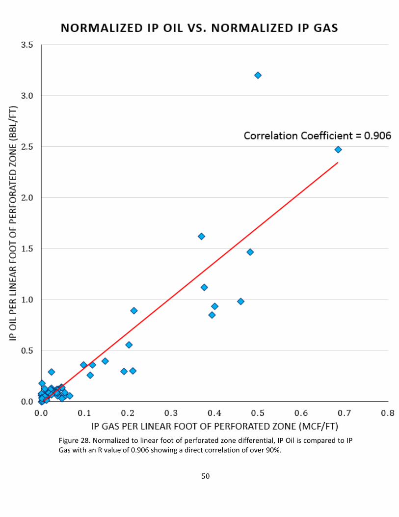
wells with productive intervals averaging around 4,000’. After normalizing the initial

production to the length of the productive zone of the wellbore, Figure 28 shows the

normalized IP oil and IP gas to be more interrelated than we initially thought. (Figure

28) shows a correlation coefficient of 0.906 which means the corrected data are

actually correlated at just over 90%. In order to correct for the incongruence in values

between wellbore types, directional and horizontal wells are looked at independently

in figures 29 and 30, respectively. Figure 29 shows the directional wells data for

normalized IP oil vs IP gas with an R value percentage of 84%. Independent of the

horizontal wells, the value still shows a strong correlation between methane and IP

oil. The equivalent cross-plot using the horizontal wells data shows a correlation

percentage of 88%, even greater than the directional wells. The shear difference in

normalized values between the two well types forced the trend line to show a higher

overall value of 91%. With each well type analyzed separately, we gain a better

understanding of the actual data less the interference due to the normalized value

disparity.

49

These data demonstrate that with more oil production, there is more gas production

fueling the transport to the surface through the production casing. Whether higher

oil mobility through viscosity reduction, or methane gas drive from de-pressuring the

reservoir, the methane in the reservoir directly affects the amount of produced oil. A

more in-depth reservoir engineering study would have to be done to prove which

function the methane plays in this particular reservoir, with current depletion and

cumulative production curves taken into consideration.

50

Figure 28. Normalized to linear foot of perforated zone differential, IP Oil is compared to IP Gas with an R value of 0.906 showing a direct correlation of over 90%.

51

Figure 29. Initial production of oil versus initial production of gas are each normalized to linear feet of the perforated interval in directional wells only. The correlation coefficient is .836 for an R value percentage of 84%.

52

Figure 30. Initial production of oil versus initial production of gas are each normalized to linear feet of the perforated interval in the horizontal wells. The correlation coefficient is .879 for an R value percentage of 88%.

53

Gas- oil ratio or GOR, as it is commonly referred to, is the gas volume in cubic feet divided

by oil produced in barrels. Before a reservoir’s pressure drops below the bubble point, a

higher GOR can be expected, as all the gas is dissolved in the oil. Generally, anything above

600 GOR is considered a gas well. Upon reaching and falling below the bubble point, gas is

liberated from the oil and a gas cap forms, forcing the GOR to change. The GOR change will

typically be related to where in vertical section of the reservoir the perforations are located.

Figure 31 shows the GOR for the Shafter Lake Field study area with no strong data points

indicating a specific area of high GOR.

Oil-cut is represented by figure 32, with the greatest percentage of oil-cut being in the

directional well territory. Oil-cut is calculated by dividing oil produced by the oil + water

produced. This gives the percentage of produced oil out of the total liquids produced. Figure

32 shows the highest oil-cut region as the eastern –northeastern section of the study area.

54

Figure 31. The gas-oil ratio or GOR is calculated by dividing IP gas values in cubic feet by IP oil values from the 24-hour tests. The midpoints of the wellbores are used as the data points.

Gas-Oil Ratio (GOR)

55

Figure 32. Oil-cut is demonstrated by dividing IP oil by (IP oil + IP water). This shows how much of the percentage of total liquid produced is oil. The midpoint of the wellbores are used as the data points.

Oil-Cut (%)

56

RESULTS

Chromatograph analysis of associated petroleum gases were taken at the wellhead of some

of these wells during the 24-hour testing interval, and after averaging the numerical results

of the highest constituents, methane came in at just over 66% (Figure 11). The individual

wells did not vary enough in concentration or geographic location to have significant

outliers, and as a result, the average percentages were considered level for all wells in the

study area.

This study shows a correlation between reservoir gas levels and initial oil produced in the

24-hour production test window reported by the drilling operator (Figure 20). Sixty-two

wells in blocks 13 and 14 of the study area were used and compared together in a cross plot

shown in Figure 20. A positive trending slope is shown by the blue markers, except for some

outliers, which are expected. These markers have a correlation coefficient of .564 and

represent the wells and how they produced in the initial 24-hour testing window. Figure 21

shows a cross plot of IP (Oil + Water) versus IP Gas with a correlation coefficient of .362.

This study focuses on oil production, but associated water with the San Andres formation is

too significant to overlook. Figure 18 shows the extent of initially produced water from

these San Andres wells.

Out of the sixty-two wells, nineteen of them were directional wells, and the remaining

forty-three wells were drilled horizontally. The much shorter directional wells produced

higher normalized rates of oil, but the shear difference in a 200’ and a 4,000’ productive

zone makes this data seem obsolete. Saving money on a shorter directional well will return

57

the highest bbl/ft of linear perforated zone (Figure 26), but oil companies want higher

volumes, not necessarily better ratios, if their competitors are bringing in 3x the amount of

actual oil. An attempt was made at differentiating vertical section units in the San Andres

Formation based on initial production and the wells behavior, but the results are

inconclusive. The directional wells targeted a lower zone on average than the horizontal

wells (Figure 22), but there is no definitive proof thus far from this study of different

stratigraphic units existing in the Shafter Lake field. The lower total depth of the directional

wells could be rat-hole drilled at the end of the well, which is common practice in vertical,

directional, and horizontal wells. However, in the horizontal wells, the rat-hole is drilled at

the end of the well laterally, as opposed to vertically in vertical and directional wells. This

rat-hole is typically drilled 150-300 feet further than the target zone, and could explain the

average difference in TVD of the directional and horizontal wells.

In Figure 28, the oil and gas levels were divided by the length of the perforated interval of

the productive zone of the wellbore and compared, effectively leveling the field of the

longer horizontals to the shorter length of the directional wells. These data clearly confirm

that oil produced is related to gas in the reservoir.

58

CONCLUSION

Correction for the productive zone of the sixty-two wellbores in the study area shows a

correlation coefficient of IP oil versus IP gas at just over 90%, which confirms that the

amount of gas is directly correlated to the amount of oil initially produced in the San Andres

Formation in the Shafter Lake field, northern Andrews County, Texas. Upon separating the

directional wells and the horizontal wells with the same normalized criteria and evaluating

independently, the R value percentages were 84% and 88%, respectively. Thus, the

hypothesis that methane is related to initial oil production has been proven correct.

However, it is uncertain whether oil mobility is caused by gas-cut saturation or the de-

pressuring of the reservoir, to form a gas cap drive.

59

REFERENCES

Ball, M. M., (2006). Permian Basin Province (044).

Blakely, R., 2013, Global Paleogeography, Deep Time Maps, Colorado Plateau Geosystems Inc. http://jan.ucc.nau.edu/~rcb7/globaltext2.html, accessed October 15, 2017.

Dandekar, A. Y., 2013, Petroleum Reservoir Rock and Fluid Properties, Second Edition. CRC Press, 2013.

Dutton, S. P., E. M. Kim, R. F. Broadhead, W. D. Raatz, C. L. Brenton, S. C. Ruppel, and C. Kerans, 2005, Play analysis and leading-edge oil-reservoir development methods in the Permian Basin; increased recovery through advanced technologies: AAPG Bulletin, v. 89, p. 553-576.

Economides, M. J., Watters, L. T., Dunn-Norman, S., Petroleum Well Construction, John Wiley and Sons Ltd., West Sussex, England, 1998.

Glenn, S. E., and Jacka, A. D., 2018, Deposition, diagenesis, and porosity history of San Andres Formation, Shafter Lake Field, Andrews County, Texas.

Hills, J., 1984, Sedimentation, Tectonism, and Hydrocarbon Generation in Delaware Basin, West Texas and Southeastern New Mexico. AAPG Bulletin, 68-3, 250-267.

Hoak, T.; Sundberg, K. & Ortoleva, P. Overview of the structural geology and tectonics of the Central Basin Platform, Delaware Basin, and Midland Basin, West Texas and New Mexico, report, December 31, 1998; Germantown, Maryland. (digital.library.unt.edu/ark:/67531/metadc678963/: accessed March 29, 2018), University of North Texas Libraries, Digital Library, digital.library.unt.edu; crediting UNT Libraries Government Documents Department.

60

Horak, Ralph L., 1985, Tectonic and Hydrocarbon Maturation History in the Permian Basin. 83, 124-129.

Melzer, S., Vance, D., Trentham, B., 2011, Report on the Potential of Residual Oil Zones in the San Andres. 2011 CO2 Conference. 3-6 p.

Ramondetta, P. J., 1982, Genesis and Emplacement of Oil in the San Andres Formation, Northern Shelf of the Midland Basin, Texas. Report of Investigations No. 116, 223 p.

Rodriguez, Lucia M., Gong, Changrui, 2017. San Andres Play in the Northwest Shelf of the Permian Basin: A New Insight on Its Petroleum Systems from Oil Geochemistry. Search and Discovery Article #10960.

Ruppel, S. C., and Cander, H. S., 1988, Effects of Facies and Diagenesis on Reservoir Heterogeneity: Emma San Andres Field, West Texas: The University of Texas at Austin, Bureau of Economic Geology, Report of Investigations No. 178, 67 p.

Sutton, L., 2014, The Midland Basin vs. the Delaware Basin – Understanding the Permian. Permian Basin, Petroleum Geology. Published in Drilling Info. https://info.drillinginfo.com/midland-basin-vs-delaware-basin/ Accessed January 27, 2018.

University Lands Website, 2018, http://www.utlands.utsystem.edu/WellLibrary

Warren, J., 2014, Top Texas Oil Producer Occidental Petroleum in the Permian, pt 2: After the Call. https://seekingalpha.com/article/1985371-top-texas-oil-producer-occidental-petroleum-in-the-permian-part-2-after-the-call Accessed November 2, 2017.