the trimmed iterative closest point algorithm - u … · contents 2 alignment of two roughly...
TRANSCRIPT

Image and Pattern Analysis (IPAN) GroupComputer and Automation Research Institute, HAS
Budapest, Hungary
The Trimmed Iterative Closest Point Algorithm
Dmitry Chetverikov and Dmitry Stepanov
http://visual.ipan.sztaki.hu

2
Contents
• Alignment of two roughly pre-registered 3D point sets
• Iterative Closest Point algorithm (ICP)
• Existing variants of ICP
• Trimmed Iterative Closest Point algorithm (TrICP)
◦ implementation◦ convergence◦ robustness
• Tests
• Future work

3
Euclidean alignment of two 3D point sets
• Given two roughly pre-registered 3D point sets, P (data) and M (model), findshift & rotation that bring P into best possible alignment with M. BB
• Applications:
◦ 3D model acquisition – reverse engineering, scene reconstruction◦ motion analysis – model-based tracking
• Problems:
◦ partially overlapping point sets – incomplete measurements◦ noisy measurements◦ erroneous measurements – outliers◦ shape defects
Note: We consider Euclidean alignment. Other alignments, e.g., affine, are alsostudied.

4
Iterative Closest Point (ICP) algorithm
Besl and McKay (1992): Standard solution to alignment problem.
Algorithm 1: Iterative Closest Point
1. Pair each point of P to closest point in M.
2. Compute motion that minimises mean square error (MSE) between paired points.
3. Apply motion to P and update MSE.
4. Iterate until convergence.
Chen and Medioni (1992): A similar iterative scheme using different pairingprocedure based on surface normal vector.We use Besl’s formulation: applicable to volumetric measurements.

5Properties of ICP
• Pre-registration required:
◦ manual◦ known sensor motion between two measurements
• Point pairing:
◦ computationally demanding◦ special data structures used to speed up (k-D trees, spatial bins)
• Optimal motion: closed-form solutions available
• Proved to converge to a local minimum
• Applicable to surface as well as volumetric measurements
• Drawbacks:
◦ not robust: assumes outlier-free data and P ⊂M◦ converges quite slowly

6Closed-form solutions for optimal rigid motion
• Unit Quaternions (Horn 1987): used by original ICP and our TrICP
• Singular Value Decomposition (Arun 1987)
• Orthogonal Matrices (Horn 1988)
• Dual Quaternions (Walker 1991)
Properties of the methods (Eggert 1997)
Method Accuracy 2D Stability∗ Speed, small Np Speed, large NpUQ good good fair fairSVD good good fair fairOM fair poor good poorDQ fair fair poor good
∗Stability in presence of degenerate (2D) data.

7
Existing variants of ICP
Goal: Improve robustness and convergence (speed).Categorisation criteria (Rusinkiewicz 2001): How variants
1. Select subsets of P and M• random sampling for a Monte-Carlo technique
2. Match (pair) selected points
• closest point• in direction of normal vector: faster convergence when normals are precise
3. Weight and reject pairs
• distribution of distances between paired points• geometric constraints (e.g., compatibility of normal vectors)
4. Assign error metric and minimise it
• iterative: original ICP• direct: Levenberg-Marquardt algorithm

8Robustness and convergence: critical issues
ICP assumes that each point of P has valid correspondence in M.Not applicable to partially overlapping sets or sets containing outliers.
Previous attempts to robustify ICP: Reject wrong pairs based on
• Statistical criteria. Monte-Carlo type technique with robust statistics:
◦ Least median of squares (LMedS)◦ Least trimmed squares (LTS)
• Geometric criteria. For example, Iterative Closest Reciprocal Point (Pajdla 1995)uses ε-reciprocal correspondence:
◦ if point p ∈ P has closest point m ∈M, then◦ back-project m onto P by finding closest point p′ ∈ P◦ reject pair (p,m) if ‖p− p′‖ > ε
Heterogeneous algorithms: heuristics combined, convergence cannot be proved.

9Robust statistics: LMedS and LTS
Sort distances between paired points, minimise
• LMedS: value in the middle of sorted sequence
◦ operations incompatible with computation of optimal motion
• LTS: sum of certain number of least values (e.g., least 50%)
◦ operations compatible with computation of optimal motion◦ better convergence rate, smoother objective function
Previous use of LMedS and LTS: Randomised robust regression
• estimate optimal motion parameters by repeatedly drawing random samples
• detect and reject outliers, find least squares solution for inliers
Robust to outliers, but breakdown point 50% ⇒ minimum overlap 50%.

10
Trimmed Iterative Closest Point
Assumptions:
1. 2 sets of 3D points: data set P = {pi}Np1 and model set M = {mi}Nm1 .
(Np 6= Nm.) Points may be surface as well as volumetric measurements.
2. Minimum guaranteed rate of data points that can be paired is known∗: minimumoverlap ξ. Number of data points that can be paired Npo = ξNp.
3. Rough pre-registration: max initial relative rotation 30◦.
4. Overlapping part is characteristic enough to allow for unambiguous matching∗∗:
• no high symmetry• no ‘featureless’ data
∗If ξ is unknown, it is set automatically: run TrICP several times, select best result.
∗∗Typical for most registration algorithms.

11Problem statement and notation
Informal statement: Find Euclidean transformation that brings an Npo-pointsubset of P into best possible alignment with M.
For rotation R and translation t, transformed points of P are
pi(R, t) = Rpi + t, P(R, t) = {pi(R, t)}Np1
Individual distance from data point pi(R, t) to M:
mcl(i,R, t) .= arg minm∈M
‖m− pi(R, t)‖
di(R, t) .= ‖mcl(i,R, t)− pi(R, t)‖
Formal statement: Find rigid motion (R, t) that minimises sum of least Nposquare distances d2
i (R, t).
Conventional ICP: ξ = 1 and Npo = Np.TrICP: smooth transition to ICP as ξ → 1.

12Basic idea of TRiCP: Consistent use of LTS in deterministic way.
Start with previous S′TS = huge number.Iterate until any of stopping conditions is satisfied.
Algorithm 2: Trimmed Iterative Closest Point
1. Closest point: For each point pi ∈ P, find closest point in M and compute d2i .
2. Trimmed Squares: Sort d2i , select Npo least values and calculate their sum STS.
3. Convergence test: If any of stopping conditions is satisfied, exit; otherwise, setS′TS = STS and continue.
4. Motion calculation: For Npo selected pairs, compute optimal motion (R, t) thatminimises STS.
5. Data set transformation: Transform P by (R, t) and go to 1.
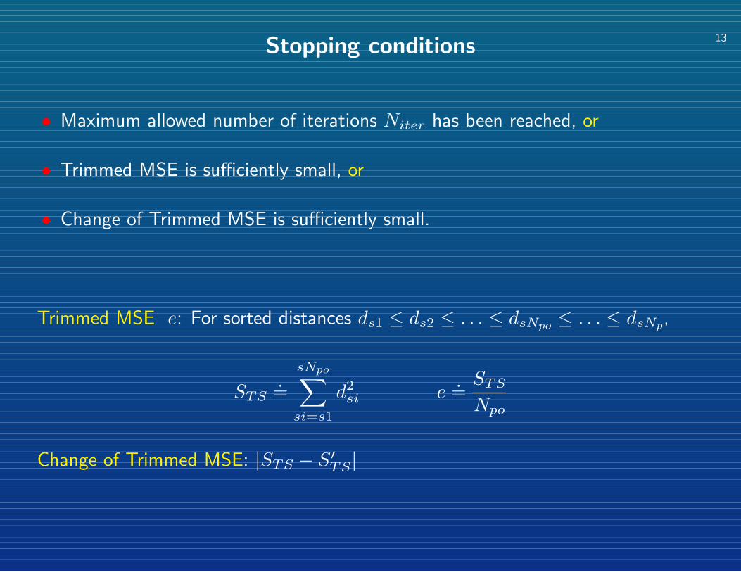
13Stopping conditions
• Maximum allowed number of iterations Niter has been reached, or
• Trimmed MSE is sufficiently small, or
• Change of Trimmed MSE is sufficiently small.
Trimmed MSE e: For sorted distances ds1 ≤ ds2 ≤ . . . ≤ dsNpo ≤ . . . ≤ dsNp,
STS.=sNpo∑si=s1
d2si e
.=STSNpo
Change of Trimmed MSE: |STS − S′TS|

14Implementation details
• Finding closest point: Use boxing structure (Chetverikov 1991) that partitionsspace into uniform boxes, cubes. Update box size as P approaches M.
◦ simple◦ fast, especially at beginning of iterations◦ uses memory in inefficient way
• Sorting individual distances and calculating LTS: Use heap sort.
• Computing optimal motion: Use Unit Quaternions.
◦ robust to noise◦ stable in presence of degenerate data (‘flat’ point sets)◦ relatively fast

15Automatic setting of overlap parameter ξ
When ξ is unknown, it is set automatically by minimising objective function
ψ(ξ) =e(ξ)ξ1+λ
, λ = 2
• ψ(ξ) minimises trimmed MSE e(ξ) and tries to use as many points as possible.
• Larger λ: avoid undesirable alignments of symmetric and/or ‘featureless’ parts.
• ψ(ξ) minimised using modified Golden Section Search Algorithm.
10 α β1
ξ
2
)(ψ)e(
ξ ξ
ξξ
Typical shapes of objective functions e(ξ) and ψ(ξ).

16Convergence
Theorem: TrICP always converges monotonically to a local minimum withrespect to trimmed MSE objective function.
Sketch of proof:
• Optimal motion does not increase MSE: if it did, it would be inferior to identitytransformation, as the latter does not change MSE.
• Updating the closest points does not increase MSE: no individual distanceincreases.
• Updating the list of Npo least distances does not increase MSE: to enter the list,any new pair has to substitute a pair with larger distance.
• Sequence of MSE values is nonincreasing and bounded below (by zero), henceit converges to a local minimum.
Convergence to global minimum depends on initial guess.
17
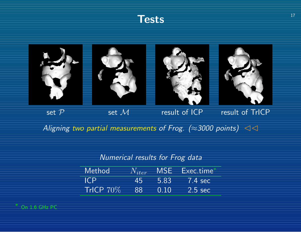
Tests
set P set M result of ICP result of TrICP
Aligning two partial measurements of Frog. (≈3000 points) CC
Numerical results for Frog data
Method Niter MSE Exec.time∗
ICP 45 5.83 7.4 secTrICP 70% 88 0.10 2.5 sec
∗On 1.6 GHz PC

18
Aligning four measurements of Skoda part. (≈6000 points)

19
Aligning four measurements of Fiat part. (overlap ≈ 20%.)

20
Aligning two measurements of chimpanzee Skull. (≈100000 points)
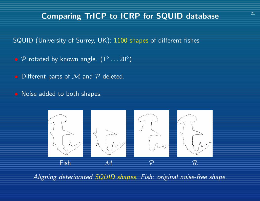
21Comparing TrICP to ICRP for SQUID database
SQUID (University of Surrey, UK): 1100 shapes of different fishes
• P rotated by known angle. (1◦ . . . 20◦)
• Different parts of M and P deleted.
• Noise added to both shapes.
Fish M P R
Aligning deteriorated SQUID shapes. Fish: original noise-free shape.

22
TrICP/ICRP errors for noisy SQUID data, degrees
100% 90% 80% 70% 60%1◦ 0.05/0.05 0.08/0.06 0.07/0.08 0.10/0.12 0.19/0.235◦ 0.05/0.05 0.09/0.07 0.08/0.11 0.12/0.18 0.34/0.31
10◦ 0.05/0.05 0.09/0.07 0.10/0.18 0.19/0.60 0.58/1.7015◦ 0.05/0.06 0.11/0.11 0.16/0.36 0.34/1.09 1.14/2.5420◦ 0.05/0.11 0.10/0.16 0.20/0.49 0.69/1.51 1.79/3.03
• ICRP is efficient at small rotations and noise-free data.
• TrICP is more robust to rotations and incomplete, noisy data. Procedure forautomatic setting of overlap available. Convergence proved.
• Execution times per alignment are comparable. Skoda 6000 pts: 8.3/7.2 sec,Skull 100000 pts: 38/182 sec.

23
Future work
• Compare to other methods for a large set of shapes.
• To better avoid local minima, perturb initial orientation of data set.
• Extension to multiple point sets N > 2.
• Faster operation.
• More efficient usage of memory.