the ttethernet synchronisation protocols and their … ttethernet synchronisation protocols and...

280 Int. J. Critical Computer-Based Systems, Vol. 4, No. 3, 2013

Copyright © 2013 Inderscience Enterprises Ltd.

The TTEthernet synchronisation protocols and their formal verification

Wilfried Steiner* TTTech Computertechnik AG, Schönbrunnerstr. 7, A-1040 Vienna, Austria E-mail: [email protected] *Corresponding author

Bruno Dutertre SRI International, Computer Science Laboratory, 333 Ravenswood Avenue, Menlo Park, CA 94025-3493, USA E-mail: [email protected]

Abstract: TTEthernet is a communication platform for critical, distributed computer-based systems. NASA has selected one of TTEthernet’s high-end configurations for the Orion programme. In other configurations, TTEthernet implements the communication backbone of new energy machineries such as wind turbines. One of TTEthernet’s unique features is the integration of applications with differing latency, jitter, and fault-tolerance requirements in a single physical Ethernet network, thereby significantly reducing the amount of wiring in a distributed system. The most critical applications can communicate using time-triggered messages for which a fault-tolerant high-precision network-wide timebase is required. Formal methods are key in the design of protocols that establish and maintain such a timebase and, thus, have been heavily used already during the design phase of TTEthernet. This paper summarises the formal analysis and verification activities of the TTEthernet synchronisation protocols and discusses protocol updates implemented in the TTEthernet standard SAE AS6802.

Keywords: clock synchronisation; fault tolerance; formal verification; model checking; TTEthernet; SAE AS6802.

Reference to this paper should be made as follows: Steiner, W. and Dutertre, B. (2013) ‘The TTEthernet synchronisation protocols and their formal verification’, Int. J. Critical Computer-Based Systems, Vol. 4, No. 3, pp.280–300.

Biographical notes: Wilfried Steiner is a Corporate Scientist at TTTech Computertechnik AG. He holds a degree of Doctor of Technical Sciences from the Vienna University of Technology, Austria. He is one of the core researchers of the TTEthernet technology and has been the Industrial Editor of the SAE AS6802 standard. He is currently also a voting member in IEEE 802.1. He has been awarded a Marie Curie Outgoing Fellowship from 2009 to 2012 hosted by SRI International in Palo Alto. His research is focused on the development of algorithms and services that enable dependable communication in cyber-physical systems and applied formal methods.

The TTEthernet synchronisation protocols and their formal verification 281

Bruno Dutertre is a Senior Computer Scientist at SRI International. He holds a PhD in Computer Science from the University of Rennes, France. He has been at SRI International since 1998. His research interests include formal method and their application to the verification of high-integrity systems. At SRI, he maintains and develops formal methods tools, including the SAL model-checking environment and the SMT solver Yices.

This paper is a revised and expanded version of a paper entitled ‘Layered diagnosis and clock-rate correction for the TTEthernet clock synchronization protocol’ presented at the 17th IEEE Pacific Rim International Symposium on Dependable Computing, Pasadena, California, USA, 12–14 December 2011.

1 Introduction

The network is a key element of many modern critical computer-based systems. Several standard solutions are available as a reliable interconnect, including, SAFEbus (Hoyme and Driscoll, 1993), TTP (Kopetz, 2002), or ARINC 664 (AEEC, 2003). However, with growing bandwidth requirements and the demand for integrating applications with different levels of criticality in a single physical network, these solutions approach their limits for a broad range of systems. This has led to the development of TTEthernet, a communication technology that aims to incorporate the best parts of the standards listed above. In addition, building on the Ethernet standard TTEthernet satisfies current bandwidth demands and supports further growth.

One core feature of TTEthernet is the support of time-triggered communication in parallel with regular Ethernet and ARINC 664-p7 frames. The dispatch times of time-triggered messages are scheduled during the system design phase. During system operation, each sender monitors the network time and dispatches a time-triggered frame whenever the current network time matches an entry in the communication schedule. The network time is thus of critical importance for time-triggered communication. Protocols that establish and maintain this network time must be in place. We call such protocols generally ‘synchronisation protocols’.

Synchronisation protocols have been rigorously studied since the 1980s (e.g., Lundelius and Lynch, 1984; Lamport and Melliar-Smith, 1984) allowing us to build on a strong scientific foundation when designing the TTEthernet synchronisation protocols. Not surprisingly, the TTEthernet synchronisation protocols share many similarities with existing ones. However, due to special characteristics of an Ethernet network and our fault model, none of the existing protocols could have been reused directly.

The design of fault-tolerant protocols in general is a non-trivial task as edge cases tend to be overlooked and implicit assumptions may not be correct. Hence, the use of formal methods in the verification process of synchronisation protocols for critical computer-based systems is imperative. While traditionally theorem provers have been used as formal methods of choice (e.g., Rushby and von Henke, 1991; Shankar, 1992; Miner, 1993; Schwier and von Henke, 1998; Pfeifer et al., 1999) the increasing power of model checking promises a cost-effective alternative to formal verification (e.g., Barsotti et al., 2007; Pike, 2007; Malekpour, 2007). Indeed, to our knowledge, the formal verification of the TTEthernet synchronisation protocols is the first successful model-checking study of fault-tolerant synchronisation protocols in a continuous time

282 W. Steiner and B. Dutertre

model. The model-checking approach we have pursued is not yet as general as theorem proving. Model checking forces us to examine fixed-sized versions of the protocols (i.e., with a fixed number of components and a fixed number of faults). Still, the increased automation offered by model checking makes it more accessible to practitioners and largely compensates for this reduced generality. In particular, model checking enables us to perform testing and simulation before any attempt at proving correctness, which is essential during early protocol design phases. This paper summarises these model-checking efforts and presents updates to the TTEthernet synchronisation protocols and their associated formal models.

In Section 2, we give a more detailed overview of the TTEthernet technology with a focus on an informal description of the synchronisation protocols. We then discuss the model-checking framework, which we use for simulation and formal proof in Section 3. In Section 4, we discuss for each one of the TTEthernet synchronisation protocols peculiarities in their models and verification as well as the verification results. Finally, we conclude in Section 5.

The design of the TTEthernet technology and the formal verification of its synchronisation protocols started in the early 2000s. Several papers have been published on the topic. In this paper, we consolidate the earlier publications and discuss protocol updates. References to the papers are given and explained in the relevant synchronisation protocols sections.

2 TTEthernet overview

TTEthernet is fully backwards-compatible with the well-known Ethernet standard defined by the IEEE 802.3 Ethernet Working Group. TTEthernet distinguishes two basic components: ‘end stations’ (also called ‘end systems’) and ‘bridges’ (also called ‘switches’). In addition to standard Ethernet, TTEthernet provides several services to improve its real-time and fault-tolerance performance. In particular, TTEthernet implements synchronisation protocols that establish and maintain synchronised time in the network in a fault-tolerant manner. An example TTEthernet system is depicted in Figure 1.

Figure 1 TTEthernet system with two redundant networks


As shown in the figure, the end stations are connected to fully redundant networks. In this case, network A consists of a single bridge, while network B consists of two bridges connected to each other with a multi-hop link. The synchronisation protocols exchange ‘protocol control frames’ (PCFs) between end stations and bridges in order to establish a synchronised timebase in the system. The PCFs follow the standard Ethernet frame format and as a most basic rule, all end stations always send their PCFs to all their connected networks.

Network components may fail, and TTEthernet is designed to tolerate failure of bridges or end stations. The failure model of the TTEthernet bridges is inconsistent-omission. Faulty bridges may loose frames or may relay frames only on a varying subset of their outgoing ports, but they cannot generate incorrect frames on their own or change the temporal behaviour of frames. This is a relatively weak failure model that needs to be justified for critical industries such as space or aerospace missions. For this reason, TTEthernet specifies a self-checking design for the bridges: a bridge can be composed out of two entities, called a ‘commander’ and a ‘monitor’. These two entities are designed to prevent fault propagation. The monitor continuously checks the behaviour of the commander and intercepts faulty frames whenever a faulty commander attempt to send them. The failure model of end stations is either inconsistent-omission, as discussed above, or fail-arbitrary. The latter is assumed for end stations that are not designed as self-checking pair. If faulty, such an end station may exhibit arbitrary frame loss (as in the inconsistent-omission model) but it may also generate faulty messages. In this configuration, however, TTEthernet is designed to tolerate either the failure of a bridge or an end station, but not multiple failures at the same time. If end stations have inconsistent-omission failures, then TTEthernet can tolerate two simultaneous component failures.

2.1 Communication options in TTEthernet

TTEthernet uses fault-tolerant synchronisation protocols to realise time-triggered communication. In this paradigm, the points in time when end stations initiate the transmissions of frames are scheduled a priori. During system operation, the end stations continually monitor the current time of the synchronised timebase. Whenever the current time matches a pre-scheduled transmission event, the end station places the corresponding frame in its outgoing queue. Likewise, the points in time when the network bridges relay the frames are also pre-scheduled. This communication plan, the ‘schedule’, coordinates the use of the network between the different end stations. For example, it can be guaranteed that the frames originated by an end station A will never compete for relay with the frames of another end station B. This systematic removal of the frame-contention problem from different end stations ensures that the transmission jitter of all time-triggered frames is minimal. Typically, the schedule is also constructed in a way that minimises transmission latencies.

In TTEthernet, frames may not only be transmitted according with the time-triggered paradigm, but end stations may also send event-triggered frames. Event-triggered communication is the classical Ethernet communication model, in which an end station places a frame in the outgoing queue as soon as it becomes ready for transmit instead of waiting for a configured point in time. As the transmission of event-triggered frames is not coordinated between different end stations, the transmission latency and jitter of


event-triggered messages will be much higher than for time-triggered messages. However, there are different types of event-triggered traffic and, for some, latency and jitter bounds can be calculated. For example, the aerospace version of TTEthernet supports standard best-effort Ethernet communication – which provides no guarantees on jitter or latency – and the ARINC 664-p7 communication paradigm (also called rate-constrained traffic) for which one can compute bounds on worst-case latency and jitter.

The synchronised timebase supports the integration of time-triggered and event-triggered traffic on a single physical network. The schedule defines the points in time when time-triggered frames are dispatched. It also implicitly defines those durations on the timeline that are free of time-triggered communication. Event-triggered traffic is then free to use these idle intervals in the schedule. In addition, the TTEthernet equipment is capable of recovering the bandwidth that is allocated to time-triggered communication but not used, for event-triggered communication.

2.2 TTEthernet synchronisation protocols

The synchronisation protocols consist of state machines in the end stations and the bridges. The goal of the protocols is to synchronise all the states in these different components. In each component p, a specific timer denoted by clockp is p’s local clock. This clock gives p a local view of the global timebase. A major goal is to ensure that the local clocks are always in approximate agreement: at any point in real-time, clockp reads almost the same value as the local clock clockq in any other component q. Formally, we write |clockp – clockq| < π, where π is called the precision in the system. The precision π is the primary parameter of the synchronisation quality.

In the following subsections, we briefly discuss the TTEthernet synchronisation protocols in an informal way. A formal treatment follows in the next sections.

2.2.1 Permanence function

The synchronisation protocol state machines exchange PCFs to coordinate their actions. These PCFs must be integrated in the network together with time-triggered and event-triggered traffic. Furthermore, as a design decision, TTEthernet allows event-triggered communication in the absence of a synchronised time. Thus, TTEthernet is ‘always up’ and ready for communication. The downside of this feature is that the PCFs may collide with event-triggered messages on the network. PCFs are typically assigned the highest priority in the network. Hence, on each outgoing port, a PCF may be delayed by the transmission of an event-triggered frame plus all other PCFs that pass the same port. These delays increase with the number of hops as a PCF is sent through the network. If these delays are not corrected for, they directly degrade the synchronisation quality, as a receiver cannot distinguish between the communication jitter of a PCF and the associated remote clock state of the sender. TTEthernet solves this problem by implementing so-called ‘transparent clocks (TCs)’ and a mechanism called the ‘permanence function’.

TCs are a well-known mechanism, implemented, for example, in the IEEE 1588 clock synchronisation standard. For this mechanism, each PCF includes a field called the TC in its payload. As the PCF is transmitted through the network, each bridge that it passes measures the duration from reception until relay. This duration and a statically


configured parameter is then added to the PCF’s current TC and updated in the TC field. This TC update is done on-the-fly when the bridge relays the PCF. The original sender of the PCF may set the TC value to a non-zero value to account for delays in the sender. Such delays may include normal processing time between dispatch and start of actual transmission, plus a possible queuing delay incurred if the sender’s output port is occupied by an event-triggered frame. Likewise, the receiver of the PCF may do a final TC update accounting for delays on the last hop. A receiver of a PCF, thus, can directly extract a PCF’s actual transmission delay TCact from its TC field.

The transparent-clock mechanism allows us to track the network latencies of PCFs. However, the communication jitter of the PCFs is of the same order of the network latency. In the best case, the PCF is never delayed by any other frame; in the worst case, the PCF is delayed by a timed-triggered frame of maximal size plus other PCFs at each hop. It turns out that, for further processing of PCFs in the fault-tolerant clock synchronisation algorithms, it is practical to transform the communication jitter into network latency, which is exactly what the permanence function does.

For the permanence function, we need to first calculate offline the maximum possible value TCmax of the TC field in any PCF communicated in the system. This is a straightforward calculation when the PCFs have the highest priority in the system. The second step is executed during system operation: when the final destination of a PCF receives a PCF on one of its ports, it does not immediately use it in the clock synchronisation process, but it artificially delays the frame by the maximum TC minus the actual TC value in the PCF: dpermanence = Tmax – Tact. Once, the PCF has been delayed for dpermanence we call the PCF permanent and it can be used in the actual clock-synchronisation process.

As we will discuss in the next section, once the local clocks of the components are synchronised, the PCFs will be sent at known points in time. The receiver stores locally an expected permanence point in time for each PCF. When a PCF becomes permanent, the receiver simply compares the expected permanence point in time with the actual permanence point in time (as presented by its local clock). The difference between the two is the difference between the local clocks of the sender and the receiver.

2.2.2 Clock-synchronisation protocol

The clock-synchronisation protocol maintains the synchronised global time. This protocol operates after initial synchronisation is reached, that is, once the local clocks of the components are already synchronised with known bounds.

For this protocol, TTEthernet distinguishes between synchronisation masters (SMs), compression masters (CMs), and synchronisation clients (SCs). Typically, the SM functionality is implemented in the end stations while some of the bridges operate as CMs. For example, in Figure 1, the end stations are configured as SMs while bridges A1 and B1 are configured as CMs; bridge B2 operates as an SC.

SMs and CMs inform each other of the current value of their local clocks by exchanging PCFs. As we have discussed previously, a component obtains a precise estimate of the difference between its local clock and the local clock of a PCF sender by measuring the difference between expected and actual permanence points in time of the PCF. Thus, the exchange of PCFs is equivalent to exchanging the current values of the local clocks of the components.


Figure 2 depicts the two steps in the TTEthernet clock synchronisation algorithm. In the first step, the SMs send PCFs to the CMs. From the arrival points in time of these PCFs, the CMs extract the current state of the SMs local clocks. The CMs then execute a first convergence function, the so-called compression function (Algorithm 1). The result of the convergence function is delivered to the SMs and SCs in the form of a new PCF (the ‘compressed’ PCF). In the second step, the SMs and SCs collect the compressed PCFs from the CMs and execute a second convergence function (Algorithms 2 and 3).

Figure 2 Overview of the TTEthernet clock synchronisation algorithm

Algorithm 1 Convergence algorithm executed by CM j

1: if |SM_clock| = 1 then 2: CM_clockj ← SM_clock1 3: else if |SM_clock| = 2 then

4: 1 2_ _2_ SM clock SM clock

jCM clock +←

5: else if |SM_clock| = 3 then 6: CM_clockj ← SM_clock2 7: else if |SM_clock| = 4 then


jCM clock +←

9: else if |SM_clock| = 5 then


jCM clock +←

11: else 12: average of the (k + 1)th largest and (k + 1)th smallest clocks, where k is the number of

faulty SMs to be tolerated. 13: end if

The compression function is based on a set of clock values received from SMs. We denote these values by SM_clocki, where 1 ≤ i ≤ |SM| and we assume that the SM_clocki values are sorted in increasing order. From the received SM_clocki, a CM j uses a variant of the fault-tolerant median to calculate the new ‘compressed’ clock CM_clockj. Algorithm 1 defines this calculation as a function of the number of SM_clocki values received (denoted by the cardinality |SM_clock|). Just before the release of TTEthernet as


the SAE AS6802 standard, Dutertre et al. (2012) discovered that the initial function was sub-optimal and proposed an update for the case |SM_clock| = 5. This update has been incorporated in the standard and is reflected in Algorithm 1, line 10.

The actual compression function that executes Algorithm 1 runs asynchronous and is started with the ‘first’ SM_clock value received. We will discuss the operation of the compression function and its correctness proof in more detail in Section 4.2.

The compressed clock is delivered back to the SMs in a new ‘compressed’ PCF. The SMs can read the compressed clock value from the arrival point in time of this PCF. The compressed PCF also contains the pcf_membership_new field in its payload. pcf_membership_new is a bitvector in which each bit is assigned to a unique SM. An CM sets the bit i in this vector if the clock value from SM I – that is, SM_clocki – was included in the calculation of the compressed clock. Bit i is cleared otherwise. Because CMs are assumed to have inconsistent-omission failures, the compressed clock CM_clockj and the pcf_membership_new vector are consistent. Hence, the self-checking pair design prevents a faulty CM from setting an arbitrary number of bits in pcf_membership_new.

In the second step of the clock synchronisation algorithm, the SMs receive the compressed PCFs, extract the compressed clock values from them, and correct their local clocks. In the fault-free case, each SM receives exactly one compressed PCF per CM, from which it extracts the compressed clock values CM_clockj, where 1 ≤ j ≤ |CM|. We assume that the CM_clockj values are sorted in ascending order.

If a CM is faulty, an SM may receive at the most one compressed PCF from this CM (as the faulty CM may fail to send its compressed PCF to some SMs). Furthermore, an SM will only use a compressed PCF in its convergence function if the pcf_membership_new field has at least accept_threshold bits set. The value of accept_threshold is calculated using Algorithm 2: the SM searches for the maximum number of bits set (bits()) in any of the PCFs received from the CMs. The value of accept_threshold is then given by this maximum minus the configured number of tolerable faulty SMs. Algorithm 2 Select(CM_clock)

1: for j = 1 → |CM| do 2: if current_max < bits(pcf_membership_newj) then 3: current_max ← bits(pcf_membership_newj) 4: end if 5: end for 6: accept_threshold ← current_max – conf_faulty_SM 7: return {CM_clock | pcf_memberhip_new ≥ accept_threshold}

The SM will discard a compressed PCF that has fewer than accept_threshold bits set in the pcf_membership_new field. This mechanism ensures that an SM excludes compressed PCFs that represent relatively low numbers of SM clocks. The pcf_membership_new vector is also used in other TTEthernet algorithms such as clique detection or startup, and in network configurations that use more than one CM per channel. We do not discuss this functionality and configurations in this paper. For the analysis of the clock synchronisation algorithm, the description above is sufficient. Under the assumption of


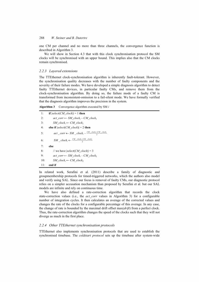
one CM per channel and no more than three channels, the convergence function is described in Algorithm 3.

We will show in Section 4.3 that with this clock synchronisation protocol the SM clocks will be synchronised with an upper bound. This implies also that the CM clocks remain synchronised.

2.2.3 Layered extensions

The TTEthernet clock-synchronisation algorithm is inherently fault-tolerant. However, the synchronisation quality decreases with the number of faulty components and the severity of their failure modes. We have developed a simple diagnosis algorithm to detect faulty TTEthernet devices, in particular faulty CMs, and remove them from the clock-synchronisation algorithm. By doing so, the failure mode of a faulty CM is transformed from inconsistent-omission to a fail-silent mode. We have formally verified that the diagnosis algorithm improves the precision in the system. Algorithm 3 Convergence algorithm executed by SM i

1: if |select(CM_clock)| = 1 then 2: act_corr ← SM_clocki – CM_clock1 3: SM_clocki ← CM_clock1 4: else if |select(CM_clock)| = 2 then

5: 1 2_ _2_ _ CM clock CM clock

iact corr SM clock +← −

6: 1 2_ _2_ CM clock CM clock

iSM clock +←

7: else 8: // we have |select(CM_clock)| = 3 9: act_corr ← SM_clocki – CM_clock2 10: SM_clocki ← CM_clock2 11: end if

In related work, Serafini et al. (2011) describe a family of diagnostic and groupmembership protocols for timed-triggered networks, which the authors also model and verify using SAL. Since our focus is removal of faulty CMs, our diagnostic protocol relies on a simpler accusation mechanism than proposed by Serafini et al. but our SAL models are infinite and rely on continuous time.

We have also defined a rate-correction algorithm that records the clock state-correction values (i.e., the act_corr values in Algorithm 3) for a configurable number of integration cycles. It then calculates an average of the corrected values and changes the rate of the clocks for a configurable percentage of this average. In any case, the change of rate is bounded by the maximal drift offset max(drift) from a perfect clock. Thus, the rate-correction algorithm changes the speed of the clocks such that they will not diverge as much in the first place.

2.2.4 Other TTEthernet synchronisation protocols

TTEthernet also implements synchronisation protocols that are used to establish the synchronised timebase. The coldstart protocol sets up the timebase after system-wide


power-on. The integration protocol allows components that are powered-on late or that are reset to join the synchronised time. Finally, the restart protocol detects if a component has lost synchronisation. These protocols are relatively simple on their own, but the interactions between all the protocols are quite complex and difficult to understand. We have used model-checking techniques similar to Steiner and Kopetz (2006) to exhaustively simulate the protocol behaviour under failure conditions. Due to the complexity of these protocols and their more traditional verification approach we do not discuss these protocols in this paper.

3 Proof and simulation framework

Our proof and simulation framework is based on the bounded model checker for infinite-state systems that is part of the SAL environment. This model checker is called sal-inf-bmc. The algorithms presented in this paper have been formalised in SAL (de Moura et al., 2004) as state-transition systems of the form ⟨S, I, →⟩. S defines the set of system states σi, I is the set of initial system states with I ⊆ S, and → is the set of transitions between system states. Each system state σ maps state variables to particular values according to their defined type. SAL supports structured modelling such that we can define the SM and CM functionality in encapsulated modules.

SAL provides several tools (symbolic, bounded, and infinite-state bounded model checking). While we experimented with all of them, we finally used the infinite-state bounded model checker sal-inf-bmc to prove the TTEthernet synchronisation protocols and to generate testcases. With sal-inf-bmc, we can treat time as a continuous entity and we can use k-induction (de Moura et al., 2003) as a proof method.

3.1 Simulation with SAL

The design of distributed algorithms is notoriously difficult, in particular in the case of fault-tolerant algorithms. The interactions of the components are hard to trace and even trivial interdependencies may not be obvious when designing an algorithm on paper. As algorithm complexity increases, analysis by means of computer-aided verification and simulation becomes more and more useful. In particular, simulation allows us to explore an algorithm’s behaviour at a very early phase of its design.

In addition to pure simulation, the model-checker approach allows us to use ‘wildcards’ for which the tool is free to assign non-deterministic values. Instead of a single simulation run that takes as input a specific test vector and analyses the system behaviour under this test, the model-checker approach systematically searches the state space for all possible valuations of each wildcard.

3.2 Formal proof with SAL

As we gain more and more trust in the design of our algorithm we also have as a goal to actually formally prove properties of interest. This is the true power of our formal framework. While we immediately deduce information through simulation, we can almost seamlessly switch to formal verification.


The proof of an invariant property P (‘P is always true’) is done by k-induction (de Moura et al., 2003), which is a generalised form of induction. k-induction consists of the following stages (Dutertre and Sorea, 2004):

• Base case: Show that all the states reachable from I in no more than k – 1 steps satisfy P.

• Induction step: For all trajectories σ0 → ··· → σk of length k, show: σ0 |= P ∧ ··· ∧ σk–1 |= P ⇒ σk |= P.

k-induction is a powerful verification tool, but it can be directly applied only to relatively simple state-transition systems. For more complex systems, we employ a proof method based on abstraction. Formally, a system-level abstraction A is also a state-transition system of the form , , ,→AS I where S is a set of abstract states Σ and ∈I S is the initial abstract state. Furthermore, →A is a set of transitions between abstract states. Each abstract state Σ represents one or more concrete states of the original system, and the system-level abstraction must fulfil the following properties.

• The initial abstract state I is the abstraction of all the initial states of the concrete system.

• For each transition in → that brings the system from a state σ1 to a state σ2, there exists an abstract transition in →A from abstract state Σ1 to an abstract state Σ2 such that Σ1 is the abstraction of σ1 and Σ2 is the abstraction of σ2.

Using the abstraction approach, the formal verification of a property P is done in two steps. In the first step, we verify that the abstraction correctly represents the model M (i.e., it satisfies the properties listed above): |=M A and in the second step we verify that the model M together with the abstraction A satisfies : | .P P∧ =M A

4 Formal verification

In this section, we discuss the formal modelling approach for the TTEthernet synchronisation protocols discussed in the previous sections. We start with the permanence function, which is the simplest protocol to model. We then discuss the compression function as a subroutine of the clock synchronisation protocol, followed by the complete clock synchronisation protocol. Finally we report how the existing models have been used to verify improved synchronisation functionality on top of TTEthernet.

4.1 Permanence function

The modelling paradigm for the permanence function represents time as real values and is based on the ‘calendar automata’ approach introduced in Dutertre and Sorea (2004). We will give an overview of the formal model and discuss the verification results. A detailed discussion of the key SAL code can be found in the CoMMiCS technical report (Steiner, 2009).

Figure 3 sketches the formal SAL model of the permanence function. It consists of three modules that represent a dispatch process, a communication channel, and the


permanence function itself. The formal model is available at the SAL wiki http://www.csl.sri.com/users/steiner/permanence.tar.gz. With respect to Figure 1, a PCF may flow from ES4 over bridge B2 to bridge B1. In this scenario, ES4 executes the dispatch process, and B1 the permanence process, while the communication channel consists of the bridge B2 and all communication links between ES4 and B1. Furthermore, an additional real-time (RT) clock module represents absolute real time, and the global data structure ‘Event Calendar cal’ is used to model the flow of a PCF from the sender to a receiver. As depicted, the permanence function is executed in the SMs and in the CMs upon reception of a PCF.

Figure 3 Overview of the formal model of the permanence function (see online version for colours)

The execution of the model is purely sequential:

• The dispatch module non-deterministically selects a dispatch timeout (dispatch timeout).

• When dispatch timeout is reached, the dispatch module transmits a PCF. This is modelled by adding an entry into the event calendar cal. At the same time, the dispatch module stores the current time in the local variable dispatch_pit.

• The entry into cal is the trigger for the channel module, which non-deterministically selects a transmission duration for the PCF (i.e., the measured transmission delay). The channel module simulates the end-to-end delay from the dispatch of a PCF until it is handed to the permanence function.

• When the channel module times out, it adds an entry into the event calendar cal. The entry includes the measured delay that models the TC field of the PCF. We distinguish two cases in the formal model: in the idealised case, we assume that the measurement is perfect. In the realistic case, we consider measurement errors, which


we model by yet another non-deterministic choice of a cumulative_error variable which is also added to the TC.

• The entry into cal is the trigger for the permanence module, which reads the TC value from the calendar and delays the PCF for the permanence delay dpermanence.

• Finally, when the permanence delay dpermanence expires the PCF becomes permanent at permanence_pit.

We are interested in the relation between the dispatch point in time to the permanence point in time. For this, we formulate two properties under test.

The first property to verify test says that whenever the permanence function module enters the p_permanent state, then the permanence_pit equals the original dispatch_pit plus the max_transmission_delay.

test: LEMMA system |- G(permanence_state=p_permanent => permanence_pit = (dispatch_pit+max_transmission_delay)));

We expect that this property holds in case when the system is free of cumulative error (that is, when max_cumulative_error = 0). If max_cumulative_error > 0, we weaken the property as follows:

test_cumulative: LEMMA system |- G(permanence_state=p_permanent => (permanence_pit >= dispatch_pit + max_transmission_delay –

worst_case_cumulative_error) AND (permanence_pit <= dispatch_pit + max_transmission_delay + worst_case_cumulative_error));

The test_cumulative property naturally defines an interval for the permanence_pit. The permanence function is simple enough that an abstraction proof is not

required, but a few simple lemmas are sufficient. We have formally verified lemma test (in absence of measurement errors) and test_cumulative (in presence of measurement errors). The non-deterministic selection of the dispatch timeout, the measured_transmission_delay, and the cumulative_error ensures that the proof is generally applicable.

4.2 Compression function

The compression function implements the first convergence function of the clock-synchronisation protocol depicted in Algorithm 1 in Section 2.2.2. It is implemented as a process that runs unsynchronised to the synchronised global time. This means that the compression function is started when the first PCF within one clock synchronisation period becomes permanent, rather than when the synchronised global time reaches a particular point in time.

Hence, it needs to periodically collect the current local clock values of the SMs in an asynchronous way: the first PCF marks a reference point in time for the current clock synchronisation period. The compression function then measures the permanence time of all following PCFs relative to this reference point. The collection process continues as long as a sufficiently high number of new PCFs is received within a fixed collection window, but will terminate after a maximum duration at the latest. The difficulty of the


compression function is to ensure that this collection process cannot be compromised by faulty SMs. We want to prove that a faulty SM sending a PCF too early or too late cannot cause the collection process to gather only a subset of non-faulty PCFs.

Figure 4 gives an overview of the formal model used to verify the compression function.

Figure 4 Compression function model overview (see online version for colours)

The structure of the formal model is similar to the one of the permanence function. We model a number of SMs as modules that communicate with a CM module using calendar automata as discussed previously. The progress in realtime is simulated by a dedicated real-time clock module. Again, the SMs are allowed to select a dispatch timeout that determines when they transmit their PCF: non-faulty SMs select the timeout within a given range, faulty SMs may arbitrarily select any transmission time. The formal model is available at the SAL wiki http://www.csl.sri.com/users/steiner/ttethernet-clocksync.tar.gz.

In Steiner and Dutertre (2010), we have verified some key lemmas of the compression function. Most important is the agreement lemma, which verifies that when the compression function terminates, the clock values of all correct SMs are used in the calculation of the CMs clock value.

4.3 Clock-synchronisation protocol

In TTEthernet, the clock synchronisation protocol discussed in Section 2.2.2 is periodically executed in periods, called integration cycles. Figure 5 shows an example scenario with a fast and a slow clock.

The x-axis depicts real time and the y-axis the internal clock time of a TTEthernet device. The perfect clock is plotted as a 45 degree solid line while the fast clock is depicted as a dashed line slightly above the perfect clock and the slow clock is depicted as a dotted-dashed line slightly below the perfect clock. The figure shows for each integration cycle the divergence of the fast and slow clocks from the perfect clock, and


their synchronisation at the beginning of each integration cycle. The drift from the perfect clock is a function of the length of the integration cycle and the drift rate of the clocks. Following the literature, we use Rsync for the integration cycle and ρ for the drift rate. In addition, we use a value Δerror to summarise other factors in the clock-synchronisation process (e.g., network jitter, inaccuracies from the clocks not perfectly executing the integration cycles at the same time). In general, we assume that Δerror is a rather small factor compared to the real clock drift. Hence, we use the term drift offset, or drift for short, for the sum of deviations of a clock from the perfect clock within one integration cycle:

sync errordrift R ρ= × + Δ (1)

In TTEthernet, we are interested in the precision of the non-faulty clocks, where the precision is defined as the maximum difference between any two non-faulty clocks in the system. In order to determine the precision, we do not need the actual clock readings but only the sequences of their differences to the perfect clock. Figure 6 illustrates this modelling approach. The x-axis represents alternation between clock drift and clock correction. The y-axis represents clock time deviations from the perfect clock. A step from an even to an odd x represents the clock drift over one integration cycle: the drift offset for an integration cycle i is added. A step from odd to even x models clock correction: the graph shows the maximum offset after the executing the clock-synchronisation protocol.

Figure 5 Progress in real time plotted against clock time

The TTEthernet clock synchronisation protocol has been verified using the abstraction approach discussed in Section 3 [see Steiner and Dutertre (2011a). The SAL models can be found at http://sal-wiki.csl.sri.com]. In this model, each SM is described by a state machine and all state machines are executed synchronously. For simplicity, we assume that each of these state machines has only two variables, SM_state and SM_clock,


where SM_state is either sync or send. State sync is the state of a SM immediately after synchronisation, and state send is the state immediately before synchronisation. Alternating between sync and send directly models the behaviour depicted in Figure 6. Variable SM_clock keeps track of the divergence from the perfect clock. The system state is the sum of the local states of the SMs.

Figure 6 Example execution of the TTEthernet clock synchronisation protocol in presence of a faulty CM

Figure 7 System-level abstraction for the formal proof

Figure 7 depicts a system-level abstraction for the TTEthernet clock-synchronisation protocol that fulfils the abstraction properties listed in Section 3. In this case, the abstraction is very simple and consists only of the two abstract states SMALL and BIG. BIG is an abstract state that holds when all SMs are in the sync state, while the abstract state SMALL holds when all SMs are in the send state. In the SAL model, the SMs are all initially in the sync state and they all perform their transitions synchronously, so they are either all in the sync state or all in the send state. Thus, the two abstract states SMALL and BIG capture all possible configurations of the concrete system. In addition, precision is bounded by some real constant FACTOR_small times max(drift) in the SMALL abstract state and by some other real constant FACTOR times max(drift) in the BIG state. FACTOR_small < FACTOR holds and both numbers are derived manually or by re-running


the model checking until no counterexamples are produced. These numbers depend on the number and type of failures present in the system.

For the original clock synchronisation protocol of TTEthernet, we have reported that FACTOR is between 2 and 4 (Steiner and Dutertre, 2011a). Hence, the precision in TTEthernet is in the interval [2 × max(drift); 4 × max(drift)]. The update proposed by Dutertre et al. (2012) for the case of 5 clock values in Algorithm 1 in Section 2.2.2 leads to better performance: the change improved the precision from 4 × max(drift) to (8/3) × max(drift).

4.4 Layered diagnosis and rate correction algorithms

We build on the representation of the TTEthernet clock synchronisation algorithm presented in Steiner and Dutertre (2011a) and discussed in the previous section. We treat this formal model as ‘holistic view’ in a sense that our framework does not rely on the output of these previous studies of the TTEthernet clock synchronisation algorithm, but incorporates the previous models with the new algorithms. The models can be found at http://www.csl.sri.com/users/bruno/sal/layered-algorithms.tar.gz.

We have extended the basic model of the TTEthernet clock synchronisation algorithm with a diagnosis algorithm that detects faulty CMs and excludes them from the clock synchronisation protocol. We describe an example scenario next; the full algorithm is defined in Steiner and Dutertre (2011b). The diagnosis algorithm is ‘layered’ because it is executed in addition to the basic TTEthernet synchronisation protocols (Algorithm 4 and Algorithm 5 in Figure 2). Using our formal framework, we can start by simulating the diagnosis and clock synchronisation algorithms together. Figure 8 depicts such a simulation outcome. This scenario was obtained for a system with five SMs and two CMs, where CM 1 is faulty in such a way that it may accept only a subset of SM_clock values. Hence, in general the compressed clocks, CM_clockj, produced by the CMs will be different. Figure 8 Example execution of the diagnosis algorithm as layered on top of the TTEthernet clock

synchronisation algorithm in presence of a faulty CM


Figure 8 plots the divergence of the clock times from real time as described for Figure 6. In this scenario, the clocks of SM 1-3 (denoted by clocks 1–3) have positive drift of 10 time units while the clocks of SMs 4 and 5 (denoted by clocks 4 and 5) have negative drift of 10 time units. In the first integration cycle, all SMs receive PCFs from both CMs. In the second integration cycle, all SMs except SM 2 receive PCFs from CM 1 (at x = 3). Consequently, SM 2 will correct its clock slightly differently than the remaining SMs (at x = 4). As SM 2 did not receive a PCF, it accuses CM 1 and will no longer accept PCFs from CM 1. As long as CM 1 does not fail to send a PCF to one of the other SMs, SM 2 always deviates from the remaining SMs after clock correction. However, in the fifth integration cycle (at x = 9), CM 1 does not send a PCF to SM 3, which in turn also accuses CM 1. So now, both SM 2 and SM 3 accuse CM 1 of being faulty. Based on these two accusations, all SMs exclude CM_clock1 from clock synchronisation. From the sixth integration cycle on (at x = 11), all SMs use only CM_clock2 for clock synchronisation. The inconsistent omission failure mode of CM 1 is transformed into a fail-silent failure.

Using this extended model of the TTEthernet clock synchronisation protocol we have been able to formally prove that the precision can be improved from 8

3 max( )drift× to 2 × max(drift).

Figure 9 Fault-free scenario of the layered rate-correction algorithm with stable SM clock drifts

We can also use the model of the basic TTEthernet clock synchronisation protocol to add a clock rate-correction algorithm [the detailed algorithm can be found in Steiner and Dutertre (2011b)]. Again, the rate-correction algorithm can be executed in addition to the basic TTEthernet synchronisation protocols. It is depicted as Algorithm 6 in Figure 2. In our formal analysis of the rate-correction algorithm, we use a network of five SMs and two channels, where each channel includes exactly one CM. Again, we start with some simulations to get confidence in the correctness of the design of the layered


rate-correction algorithm and in its formal model. An example scenario is presented in Figure 9.

Figure 9 plots the divergence of the clock times from real time as introduced in Figure 6. Clocks 1 to 3 have a positive drift, while clocks 4 and 5 have a negative drift. The first two integration cycles are configured as an observation phase in which the nodes record their clock correction values. After the second integration cycle, the clocks adapt the rate of their clocks. In the scenario of Figure 9, from the third integration cycle onwards, all clocks are almost perfectly aligned.

Figure 10 Fault-free scenario of the layered rate-correction algorithm with unstable SM clock drifts

The scenario discussed above is certainly idealised as it reflects the strong assumption of perfectly stable clock drifts. In reality, this will hardly be the case. Figure 10 shows a scenario with unstable clocks and resulting changing drift rates. Here, during the first integration cycle, clocks 1 to 3 have positive drift while clocks 4 and 5 have negative drift. As in the stable drift scenario, clocks 4 and 5 are the only clocks that correct their clock state. At the end of integration cycle 2, clocks 4 and 5 change their rate to reflect the previous correction (they will change their rate by +2 time units in the figure). Now, the drift of the clocks changes, in a way that clocks 1 to 3 now drift in the negative direction while clocks 4 and 5 drift in the positive direction. As a consequence, the correction value that clocks 4 and 5 apply adds to the now positive drift, which causes the precision to degrade.

Using the extended clock synchronisation model, we can formally prove that the rate-correction algorithm ensures that, even under arbitrarily changing drift rates within the specified drift range, and in presence of an inconsistent omission faulty CM, the overall precision is bounded by 8/3 × 2 × max(drift).


5 Conclusions

The design of synchronisation protocols for fault-tolerant systems is error prone and such protocols are difficult to verify. TTEthernet specifies a family of synchronisation protocols. We have described their functionality and purpose. We have discussed the permanence function as a basic building block of TTEthernet which converts communication jitter into transmission latency. The TTEthernet clock-synchronisation protocol itself consists of two convergence functions. We have discussed the first one, the compression function, in more detail because of its unique implementation characteristics. We have discussed recent updates of the TTEthernet clock synchronisation protocol, and outlined two extensions: a diagnosis algorithm and a clock rate-correction algorithm that are suitable to be implemented on top of TTEthernet.

In the design of the TTEthernet synchronisation protocols we have found formal methods not only helpful to explore and simulate alternative solutions, but even essential to taking the right design decisions. We have shown the versatility of our formal verification framework based on the bounded model checker sal-inf-bmc. The framework can be directly applied to verify simple functions like the permanence function. The manual verification overhead gradually increases with the complexity of the protocol under test as the user must find relevant lemmas or construct abstraction. Furthermore, the formal framework is easy to apply and the models are highly re-useable, as we have demonstrated with the layered extensions to the clock-synchronisation protocol.

Acknowledgements

The research leading to these results has received funding from the European Community’s Seventh Framework Programme (FP7/2007-2013) under grant agreement no. 236701 (CoMMiCS). The second author was partially supported by NASA contract NNL10AB32T and by NSF Grant CSR-0917398. The content is solely the responsibility of the authors and does not necessarily represent the official views of NASA or NSF.

References AEEC (2003) ARINC Project Paper 664, Aircraft Data Networks, Part7, AFDX Network (Draft),

Aeronautic Radio, Inc., November. Barsotti, D., Nieto, L. and Tiu, A. (2007) ‘Verification of clock synchronization algorithms:

experiments on a combination of deductive tools’, Formal Aspects of Computing, July, Vol. 19, No. 3, pp.321–341.

de Moura, L., Owre, S., Ruess, H., Rushby, J., Shankar, N., Sorea, M. and Tiwari, A. (2004) ‘SAL 2’, in Computer-Aided Verification, LNCS, Vol. 3114, pp.496–500, Springer.

de Moura, L., Rueß, H. and Sorea, M. (2003) ‘Bounded model checking and induction: from refutation to verification’, in Computer-Aided Verification, CAV 2003, Lecture Notes in Computer Science, Vol. 2725, pp.14–26, Springer.

Dutertre, B. and Sorea, M. (2004) ‘Modeling and verification of a fault-tolerant real-time startup protocol using calendar automata’, in Proc. of Formats/FTRTFT, Lecture Notes in Computer Science, Springer-Verlag, September, Vol. 3253, pp.199–214.


Dutertre, B., Shankar, N. and Owre, S. (2012) ‘Integrated formal analysis of timed-triggered Ethernet’, Contractor Report NASA/CR-2012-217554, NASA, March 2012, [online] http://ntrs.larc.nasa.gov/ (accessed 26 June 2013).

Hoyme, H. and Driscoll, K. (1993) ‘Safebus (tm)’, IEEE Aerospace and Electronics Systems Magazine, March, Vol. 8, No. 3, pp.34–39.

Kopetz, H. (2002) TTP/C Protocol – Version 1.0. TTTech Computertechnik AG, Vienna, Austria, July [online] http://www.ttagroup.org/ (accessed 26 June 2013).

Lamport, L. and Melliar-Smith, P.M. (1984) ‘Byzantine clock synchronization’, in Proc. of the 3rd annual ACM Symposium on Principles of Distributed Computing, ACM, New York, NY, USA, pp.68–74.

Lundelius, J. and Lynch, N. (1984) ‘An upper and lower bound for clock synchronization’, Information and Control, Vol. 62, Nos. 2–3, pp.190–204.

Malekpour, M.R. (2007) ‘Model checking a byzantine-fault-tolerant self-stabilizing protocol for distributed clock synchronization systems’, Technical Report NASA/TM-2007-215083, NASA.

Miner, P.S. (1993) Verification of Fault-Tolerant Clock Synchronization Systems, NASA Technical Paper 2249, NASA.

Pfeifer, H., Schwier, D. and von Henke, F.W. (1999) ‘Formal verification for time-triggered clock synchronization’, in Weinstock, C.B. and Rushby, J. (Eds.): Dependable Computing for Critical Applications 7, January, Vol. 12, pp.207–226, IEEE Computer Society.

Pike, L. (2007) ‘Modeling time-triggered protocols and verifying their real-time schedules’, in Proceedings of Formal Methods in Computer Aided Design (FMCAD’07), IEEE, pp.231–238.

Rushby, J. and von Henke, F. (1991) ‘Formal verification of the interactive convergence clock synchronization algorithm’, Technical Report SRI-CSL-89-3R, Computer Science Laboratory, SRI International, Menlo Park, CA, February 1989; Revised August 1991.

Schwier, D. and von Henke, F. (1998) ‘Mechanical verification of clock synchronization algorithms’, in Formal Techniques in Real-Time and Fault-Tolerant Systems, Lecture Notes in Computer Science, Vol. 1486, pp.262–271, Springer-Verlag.

Serafini, M., Bokor, P., Suri, N., Vinter, J., Ademaj, S., Brandstätter, W., Tagliabò, F. and Jens, K. (2011) ‘Application-level diagnostic and membership protocols for generic timed-triggered systems’, IEEE Transactions on Dependable and Secure Computing, March–April, Vol. 8, No. 2, pp.177–193.

Shankar, N. (1992) ‘Mechanical verification of a generalized protocol for byzantine fault-tolerant clock synchronization’, in Formal Techniques in Real-Time and Fault-Tolerant Systems, Lecture Notes in Computer Science, Vol. 571, pp.217–236, Springer-Verlag.

Steiner, W. (2009) ‘TTEthernet executable formal specification’, Deliverable 236701 for the CoMMiCS project1.

Steiner, W. and Dutertre, B. (2010) ‘SMT-based formal verification of a TTEthernet synchronization function’, in Formal Methods for Industrial Critical Systems, Lecture Notes in Computer Science, Vol. 6371, pp.148–163, Springer-Verlag.

Steiner, W. and Dutertre, B. (2011a) ‘Automated formal verification of the TTethernet synchronization quality’, in NASA Formal Methods (NFM’2011), Lecture Notes in Computer Science, Vol. 6617, pp.375–390, Springer-Verlag.

Steiner, W. and Dutertre, B. (2011b) ‘Layered diagnosis and clock-rate correction for the TTethernet clock synchronization protocol’, in PRDC 2011, pp.244–253.

Steiner, W. and Kopetz, H. (2006) ‘The startup problem in fault-tolerant time-triggered communication’, in Dependable Systems and Networks (DSN’2006), pp.35–44.

the ttethernet synchronisation protocols and their … ttethernet synchronisation protocols and...

Documents