the unexpected consequences of generic entry
TRANSCRIPT
ECARES ULB - CP 114/04
50, F.D. Roosevelt Ave., B-1050 Brussels BELGIUM www.ecares.org
The Unexpected Consequences of Generic Entry
Micael Castanheira SBS-EM, ECARES, Université libre de Bruxelles, CEPR, FRS-FNRS
Carmine Ornaghi
University of Southampton, UK
Georges Siotis Universidad Carlos III de Madrid, CEPR
October 2019
ECARES working paper 2019-21

The Unexpected Consequences of Generic Entry.∗
Micael Castanheira† Carmine Ornaghi‡ Georges Siotis§
September 18, 2019
Abstract
Generic drugs are sold at a fraction of the original brand price. Yet, generic entry
typically produces a drop in the quantity market share of the molecule losing exclusivity.
This effect is economically and statistically significant for a large dataset covering hun-
dreds of prescription drugs sold in the US during the period 1994Q1-2003Q4. This paper
proposes the first systematic analysis of what appears to be a market anomaly.
We propose a model to characterize the market equilibrium before and after generic
entry. We identify precise conditions under which entry reduces the quantity market
share of the molecule. Intriguingly, this is more likely to occur when the remaining
patent-protected molecules feature low horizontal differentiation. We test this and other
theoretical predictions of the model and find they are validated empirically.
JEL Classification: D22, I11, L13
Keywords: Non-Price competition, Pharmaceutical industry, Generic entry, Consumer
choice
∗This paper is dedicated to the memory of Maria-Angeles de Frutos, who passed away just after completinga closely related paper. The genesis of this paper owes a lot to her insights and enthusiasm. We wouldlike to thank two anonymous referees, the Editor, Laurent Bouton, Guilhem Cassan, Christopher Cotton,Raffaele Fiocco, Michel Goldman, Margaret Kyle, Patrick Legros, Alessandro Lizzeri, Laurent Mathevet,Jacopo Perego, Regis Renault, Patrick Rey, Pablo Querubin, Tobias Salz, Fiona Scott Morton, Denni Tommasi,and Philippe Weil for their helpful comments, as well as seminar participants at Oxford University, ECARES,i3h, the Paris School of Economics, Queen’s University, Universidad Carlos III, Universite de Cergy-Pontoise,Universite de Lausanne, EARIE2016, and CRETE2016.†ECARES (Universite Libre de Bruxelles - SBS-EM) and CEPR. Micael Castanheira is “Directeur de
recherche” FRS-FNRS and gratefully acknowledges their financial support.‡University of Southampton§Universidad Carlos III de Madrid and CEPR. Georges Siotis gratefully acknowledges the financial support
from the Ministerio Economıa y Competitividad (Spain) grants Beca I3 2006/04050/011, ECO2015-65204-P,MDM 2014-0431, and Comunidad de Madrid grant MadEco-CM (S2015/HUM-3444).

1 Introduction
The growing costs of health care and pharmaceutical treatments often make newspaper head-
lines. High hopes are generally put on the market penetration of generics to limit ballooning
drug prices. The results have been mixed: as we detail in this paper, generics indeed appear
to be very effective competitors against molecules that experience Loss of Exclusivity (LoE).
However, they typically fail to dent the position of drugs that remain on patent. As we
show below (see Figure 1, p.6) at least until 2003, generic entry was associated with a drop
in the quantity market share of the genericized (and thus cheaper) molecule. Still today,
the availability of generics fails to dampen overall expenditure growth in the US, a country
where drug prices are primarily determined by competitive interaction (see e.g. Crow, Jan.
4th, 2018). In that context, the recent record number of generics approval by the Federal
Drug Administration (FDA) praised by The Economist is welcome, but unlikely to put a
lid on prices.1 This suggests that the market wide effects of generic competition are poorly
understood.
A central characteristic of the pharmaceutical industry is the unique combination of high
investments in research and development and in promotion.2 While R&D is the driver of
market entry and of the differentiation between treatments, it is sunk by the time of generic
entry, in contrast to promotional effort. Once on the market, a firm that wants to gain
market share must either reduce its price or intensify its promotion effort. The process of
approaching doctors to tout the virtues of a treatment is known as detailing. For large players,
detailing and other forms of promotion represent 15% to 20% of total sales, about the same
as R&D. Also, detailing was a still relatively unregulated activity in the 1990s and early
2000s,3 which offers a unique opportunity to study the broader question of how promotion
1The Economist, March 24th, 2018, “Getting medicines to market faster.”2The pharmaceutical industry is indeed a particular one. In the Oxford Handbook of the Biopharmaceutical
Industry, Harrington (2012) estimates the R&D to be at 17.9% of total net sales for the period 2001-2005, andKenkel and Mathios (2012) report that the advertising-to-sales ratio was 18% in 2005 in the U.S. As pointsof comparison, they highlight that, in 2010, advertising stood at 4.5% of total net sales for General Motors(a car producer), 9.5% for Anheuser Busch (a beer producer) and 10.8% for Kellogg (breakfast cereals). Thefigures are typically smaller for most other R&D-intensive industries. For instance, in 2013, Apple spent 3%of its total net sales on R&D and 0.4% on advertising (Apple 2013: 10-K SEC submission).
3The first code of conduct of the Pharmaceutical Research and Manufacturers of America (PhRMA) tookeffect in July 2002. Direct to Consumers Advertising (DTCA) was still in its infancy.
1

affects competition in the pharmaceutical industry.
The model abstracts from the R&D decision and focuses on the period around the loss
of exclusivity (LoE) that triggers generic entry. We distinguish three phases: (1) before
generic entry, two firms, A and B, have a monopoly on their own molecule. Doctors seeking
a treatment for their patient are thus facing a differentiated duopoly. (2) One of the two
molecules, say A, loses exclusivity. We model this as a switch toward perfect competition for
market segment A, while firm B retains exclusivity. We call this an asymmetric competition
shock. (3) The third phase is when also B loses exclusivity, leading to perfect competition for
both molecules. We derive the market equilibrium in each of these three phases and identify
three main results that are important to understand the effects of generic entry—the changes
between phase 1 and phase 2 in the model.
First, generic competition for A allows B to increase its price and its market share when
the two products are close substitutes. This reverses the effects of a competition shock in
the absence of promotion. The rationale is that the more substitutable the two goods are,
the more aggressively A and B compete prior to generic entry, in phase 1. This translates
into initially lower prices and higher promotion. In that situation, generic entry has a com-
paratively small impact on prices: the reduction in promotion dominates. High levels of
differentiation have the opposite effect: prices are initially high and promotion low. Then,
generic entry primarily affects prices: both A’s and B’s prices drop.
Second, B benefits from A’s loss of exclusivity when the market is large and profitable.
The reason is that these are the markets in which firms initially invest the most in promotion
and detailing. Then again, profit erosion on the A-segment after generic entry triggers a
large drop in promotion intensity for A, which eases competitive pressure on B. Hence, the
prediction of the model is that generic competition significantly curtails B’s market share
only in small and comparatively less profitable markets.
Third, we can compare the market outcome in each of the first and second phase with
the market outcomes that would result from perfectly competitive market conditions (third
phase). Compared to that benchmark, we find that the market allocation is always worsened
by asymmetric competition: the market share of A only increases when it is already too high
in the first place, and it only decreases (to the benefit of B) when it is already too low (we
2

briefly discuss welfare in the concluding section).
Bringing these results to the data, we find that they are more than a theoretical con-
struct: using a data trove tracking prices, promotion, and quantities sold in the USA during
the period 1994-2003, we show that competition by generics in the multi-billion-dollar phar-
maceutical market often fails to put effective pressure on the drugs that remain protected by
a patent. As detailed in Section 2, despite price drops as high as 45% for the drug experi-
encing generic entry, the average effect is to boost the market share of competing molecules.
The volume market share of the molecule that is now cheaper—the originator drug plus its
chemically equivalent generic version—drops by 31% in the pharmacy channel and by 26%
for drugs sold in hospitals.
Instances of generic entry are also an ideal testing ground for technical reasons. First,
generic entry typically results from an exogenous cause: the loss of patent protection. It has a
set date, some 20 years after the patent was introduced.4 It also produces a competition shock
that is quite different from the entry of new competing products. Such a clear dichotomy
between the launch of new products and the loss of market power for a single product would
be difficult to observe in other markets. Second, agency issues between patients, physicians,
and insurances likely increase the sensitivity of demand to promotion relative to prices, which
magnifies the effects we are after.
Our sample covers all prescription sales in the U.S. between 1994Q1 and 2003Q4 (40
quarters). From that dataset, we extract all the therapeutic classes (“ATC3 markets”) for
which data on prices, quantities, and promotional efforts are available. We then cross these
data with that of the FDA to identify episodes of generic entry (see Section 4). This leaves
us with 95 episodes of generic entry scattered over 53 different ATC3 markets.
After controlling for other sources of heterogeneity, we find that, on average, generic
entry alone causes a 15% increase in market share for molecules that remain on patent. The
effect is smaller in the hospital channel: in part because of effective procurement processes,
hospitals display higher price elasticity. In line with theoretical predictions, this reinforces the
4Such a long delay also ensures that the firm’s entry decision and choice of a “horizontal location”(Hotelling, 1929) or of a “vertical differentiation” (Shaked and Sutton, 1982) are both exogenous to the char-acteristics of competition and residual market size at the time of LoE. This produces substantial exogenousvariation across episodes of generic entry, which we exploit in our empirical analysis.
3

effect of price competition–by about 4 percentage points. We also propose a novel measure
of product differentiation for the pharmaceutical industry based on the number of modes
of action within a therapeutic class. Again in line with predictions, differentiation knocks
another 4 percentage points off the market share gain of the competitors. Last, the market
share gain is further reduced by 8 percentage points in “small” markets. All these results
are more pronounced when the molecule experiencing the LoE was a blockbuster. Finally,
we explore the connection between our findings and evergreening (the presence of a second-
generation product by the same originator). In particular, in Section 6.1 we show that the
gains in market share of on-patent drugs is more pronounced when the originator company
that experiences LoE also owns patent rights on another drug in the same therapeutic market.
In other words, evergreening turns out to be a strategic complement to the promotion effects
identified by our model.
Related literature. Our paper is at the intersection of several literature strands, includ-
ing industrial organization, advertising, and health economics. With regard to our empirical
application, the existing literature on competitive interactions in the pharmaceutical industry
has produced a complex, and sometimes contradictory, picture. One group of papers analyzes
inter-brand competition when drugs are still patent-protected (see, for instance, Brekke and
Kuhn (2006) for a theoretical model and Dave and Safer (2012) for empirics). de Frutos, Or-
naghi and Siotis (2013) analyze inter-brand competition when the proportion of brand-loyal
consumers is endogenously determined by promotional effort.
Another strand focuses on intra-molecular competition following loss of exclusivity — i.e.,
when a generic bio-equivalent drug can legally come to market (e.g. Scott Morton (2000)).5
It was in that context that the “generic entry paradox” has been unearthed (the paradox
being that the price of the originator drug often goes up following the launch of a competing
chemically equivalent generic). This empirical finding has been thoroughly documented (see
a.o. Caves et al. (1991); Regan (2008); Vandoros and Kanavos (2013)).
The few papers that attempted to simultaneously analyze pre- and post-LoE competition
have produced a mixed picture. For instance, Stern (1996) provides evidence of intense inter-
5See Grabowski and Kyle (2007) for a description of generic entry in the U.S. in the period 1995-2005,and Berndt and Dubois (2016) for a comparison of generic penetration across OECD countries for the period2004-2010.
4

molecular competition, whereas Ellison et al. (1997) reports strong intra-molecular rivalry
between the originator and the generic version of the drug, as well as weak (or insignificant)
inter-molecular competition.
A related literature focuses on the relative importance of the persuasive and informative
roles of promotional effort (Ching and Ishihara (2012)) and on whether detailing and direct-
to-consumer advertising have a market expansion effect (Ching et al. (2016); Iizuka (2004,
2005); Fischer and Albers (2010)). Mizik and Jacobson (2004) analyze the effectiveness of
promotional effort by estimating the long-run effect of detailing and sampling on prescrip-
tions for three drugs. Manchanda, Rossi and Chintagunta (2004) assess whether, from a
business perspective, detailing is misallocated across individual physicians. Narayanan and
Manchanda (2009) show that the persuasive effect dominates at the end of a molecule’s
exclusivity period.
Huckfeldt and Knittel (2011) show that evergreening strategies (the launch of a second-
generation product by the same originator) helps explain instances of volume market share
drop of the previous generation molecule, despite being sold at a fraction of the original
price. Lakdawalla and Philipson (2012) share our motivation (volume sales drop following
LoE) and exploit a similar sample. The main difference lies in the fact that we explicitly
model competition, and derive testable implications that help explain the heterogeneity in
market reactions they identify.
The remainder of the paper is organized as follows. Section 2 presents some facts central
to our research question. Section 3 presents the model and derives testable implications.
Section 4 describes the data, while Section 5 presents the empirical results. Section 6 reports
robustness and sensitivity checks. Section 7 concludes by discussing how the presence of non-
price instruments can lead to mismatch between consumers and goods when competition is
asymmetric.
5

2 Generic competition: some empirical regularities
2.1 Price, patents, and quantities
Here, we detail our claim that, while generic entry produces a dramatic change in competitive
conditions, its effects substantially deviate from the predictions of elementary models of
industrial organization.
The expected effect is as follows: generics being typically sold at a fraction of the price
of the original brand, they exert strong competitive pressure on the originator: Grabowski et
al. (2014) show that, for branded drugs facing generic entry in 2011-2012, brands retained on
average only 16% of the molecule market after one year. Figure 1 provides another perspective
on these evolutions. Lumping together the original brand and its generic equivalents, it
depicts the evolution of the mean and median price and quantity for the 95 molecules that
experienced generic entry in our dataset (U.S. data for the period 1994Q1-2003Q4). Time
is expressed in quarters, and we denote as “date 0” the quarter in which molecules lose
exclusivity. We normalize to 1 values at quarter −12.
Figure 1: Price and Quantity around generic entry. Quarter-by-quarter evolution of themean and median Price and Quantity for the 95 molecules that experienced generic entry in ourdataset (U.S. data for the period 1994-2003; quarter 0 identifies generic entry).
6

What stands out is that, within a year of the Loss of Exclusivity (LoE), mean (respectively,
median) prices drop by about 30% (20%). Within three years, the drop reaches about 50%
(40%).6 In spite of this, sales in volume drop, on average, by more than 25% within three
years of patent expiry.7 As our econometric analysis will show, this means that generic entry
mainly benefits competing molecules. Put differently, few new patients are directed to the
cheap genericized molecule, and a number of existing patients switch to competing molecules
just when their treatment becomes cheaper. Neither the rationales for the generic entry
paradox nor third party payer reimbursement rules can explain why cross-price elasticities
suddenly seem to take the “wrong sign”.
2.2 Loss of exclusivity and promotion intensity
Turning to promotion, Figure 2 shows that LoE also triggers a major drop in the firms’ pro-
motional effort (we will use the terms detailing, promotion and advertising as synonymous).
Using data from IMS-Health, we measure the firms’ drug-specific spending on personalized
visits to general practitioners and hospital specialists, free samples dispensed to physicians,
and advertising in professional journals. All these instruments affect the physicians’ incentives
to prescribe one drug rather than another. The data reveal that promotion falls continuously
over the 12-quarter period before patent expiration, with a sharp acceleration around the
time of LoE. At time 0, promotion effort already dropped by 50%. Four quarters later, the
median drop is close to 95%. At 12 quarters after LoE, median spending is zero.8
The fact that price and promotion dynamics may have offsetting effects was already
6Although the average price of the molecule (displayed) falls following generic entry, this is not always thecase for the price of the branded drug (not separately depicted in Figure 1). Sometimes, the latter remainsconstant or even increases; this is the so-called generic entry paradox (for empirical evidence, see Regan (2008)for the U.S. and Vandoros and Kanavos (2013) for the EU). This behavior is usually attributed to the factthat a subset of patients insist on purchasing the brand, even at a higher price. This allows branded producersto keep extracting rents on a (shrinking) subset of patients.
7The only significant exception pertains to the quarter of when generics enter the fray. Lakdawallaand Philipson (2012)’s monthly data show that 60% of the molecules gain volume in the first two monthssurrounding generic entry (see their Figures 1 and 7). However, these gains are reversed by month 4. Stockadjustments may be one of the drivers of this increase.
8The average lies above the median because some molecules continue to be promoted. For instance,high levels of promotions are observed for Prozac (fluoxetine) because Eli Lilly & Co. introduced weeklydelayed release capsules of the drug just before LoE in an attempt to stem the post-patent decrease in sales oftheir daily dosage. Similarly, we observe positive spending for Zantac (ranitidine) and Tagamet (cimetidine),probably because some of their lower-dosage tablets are available over-the-counter (no prescription required).
7

Figure 2: Price and Promotion around generic entry
emphasized by Caves, Whinston and Hurwitz (1991). However, they did not explore the
matter further, either theoretically or empirically. Subsequent empirical research confirmed
that sales may increase or decrease: Berndt et al. (2003), Lakdawalla et al. (2007), and
Lakdawalla and Philipson (2012, Figures 7 and 9) find that the volume of sales does not
increase after LoE, and that firms cut down on promotion effort. Aitken et al. (2009, 2013)
report increased sales. Duflos and Lichtenberg (2012, p95) find that “the net effect of patent
expiration on drug utilization is zero”.
However, the literature falls short of explaining when and why one or the other outcome
should materialize, or even if these apparently haphazard evolutions really are the result of
the tension between prices and promotion. Our purpose is to investigate that very question.
2.3 Generic Entry vs. Evergreening?
Before moving to the formal analysis of that question, we briefly discuss evergreening strate-
gies, a candidate explanation for the phenomena described in the previous section. Ever-
greening consists in the launch of new formulations or second-generation versions of a drug,
leading to “product hopping” by patients (see Huckfeldt and Knittel (2011) for a detailed
8

analysis). The logic is for the firm losing exclusivity on some drug A to launch a “new” drug
A′ and stimulate patients’ migration before LoE. When successful, this shrinks the market
share of the original product, leaving generic entrants little to compete for.9
While we acknowledge that this can be an important driver of the transfer to “new”
molecules, we show in Section 6.1 that evergreening is not a substitute to the effect we
identify. First, because only a fraction of the LoE episodes in our dataset could be associated
with evergreening. Our empirical results are robust to the exclusion of these episodes. Second,
an effective promotion strategy is necessary to organize the patient migration towards the
second-generation product. The fact that the firm losing exclusivity and the firm proposing
a replacement drug are one and the same should only make promotion more effective. This
is exactly what we report in Section 6.1.
3 The model
To analyze the effects of generics entry, we build on a textbook model of differentiated
Bertrand competition with advertising. That is, (1) initially, two firms sell differentiated
drugs and compete through price and promotion. In contrast with the standard textbook
approach, we consider (2) a competition shock that is highly asymmetric: a generic is a
perfect substitute for one molecule in an otherwise horizontally differentiated industry. (3)
In the spirit of Inderst and Ottaviani (2012), consumer decisions are mediated through in-
termediaries who can be persuaded to modify their purchasing recommendations. In our
framework, however, this is only relevant for the normative analysis: realized consumption
decisions may differ from those that would maximize the utility of the final consumer.
While our textbook model overlooks interesting complexities of pharmaceutical markets, it
clarifies that our results are exclusively driven by the interaction between price and promotion
9The EU Commission’s Sector Inquiry (2009) gathered evidence on the tactics deployed to support ev-ergreening. One EU national authority reported that: “In fact, there are special strategies linked to patents,which can constitute barriers to entry for generics. A quick legal research allowed [us] to supply a few ex-amples: Modification of composition of the pharmaceutical specialty; Extension of therapeutic indication [...];Launching of an enantiomer; and registering a patent as regards a new formulation, which is presented as moreefficient.” (Sector Inquiry -SI-, p.358, #1019). A wholesaler noted that “[...] originator companies have at-tempted to reduce the impact of pending generic competition by introducing apparent last minute improvementsto products, or by changing the galenic form of their molecule.” (SI, p. 358, #2021).
9

strategy. We further discuss our assumptions at the end of this section.
Two firms, A and B, initially compete both in prices p and in “advertising,” a – or any
other fixed cost that stimulates demand. We then study the effects of the entry of one or
more generic firms, G, that produce a perfect substitute for firm A’s drug – note that we
are not contemplating evergreening strategies, nor the launch of a “branded” or “authorized”
generic. Intuitively, substitutability implies that A’s advertising effort produces a positive
spillover on G. However, competition between A and G causes both the price and advertising
effort of A to drop. Our central question is: what happens to the demand for B?
Formally, we derive the firms’ promotion and pricing strategy given the quality θJ of
their molecule, the heterogeneity of treatment responses across patients, e,10 and the agents’
sensitivity to price, δ.11 In the spirit of Shaked and Sutton (1982), consider a patient i
who goes to her physician with a condition that requires treatment. The intrinsic utility of
the Patient-Physician-Payer triplet (“P3” henceforth)12 i’s from using treatment A or B is,
respectively (we introduce advertising below):
U iA = θA − δpA + εi, (1)
U iB = θB − δpB − εi, (2)
where pJ is the price of molecule J ∈ {A,B}; εi ∼ U[− e
2 ,e2
]is the relative efficiency of drug A
as opposed to B to treat patient i’s condition; and U[.] denotes the uniform distribution.13 A
larger value of e implies that patients are more heterogeneous in their response to treatments,
and hence that the two molecules are more distant substitutes. The parameter δ accounts for
their price sensitivity.
10 These parameters directly relate to vertical and horizontal product differentiation in classical industrialorganization analyses. However, product differentiation is not a choice variable in our model.
11This model specification fits the industry’s description provided by Berndt (2002): “Within many ther-apeutic classes of drugs, a number of possible substitute medications exist, and in such cases, the marketstructure is more appropriately depicted by the differentiated product oligopoly framework. In such a set-ting, it is useful to envisage the optimal profit maximizing price as equaling marginal cost plus a positivemargin, where the margin depends on benefits and attributes (including prices) the firm’s own drug relativeto other drugs in the therapeutic class, on attributes of non-drug therapies, patient heterogeneity and otherdemand-side considerations.”
12The “payer” can be a Third Party Payer (TPP), patient out-of-pocket expenditure, or a combination.13Focusing on a single random variable ε that can be either positive or negative implicitly eliminates patients
with negative valuations of the two molecules, who have no reason to consume either of the two drugs. Thus,issues of aggregate under- or over-prescription are beyond what this model can capture.
10

Horizontal differentiation implies that patients with a sufficiently good fit with drug A
(i.e., with εi sufficiently positive) buy treatment A, and the others buy drug B.14 Letting
µ denote market size (or the number of afflicted patients), we identify the patient i who is
indifferent between A and B to determine quantities in the absence of detailing:
QA =
(1− F
(∆θB − δ∆pB
2
))× µ
QB = F
(∆θB − δ∆pB
2
)× µ,
where F represents the CDF of εi, ∆θB ≡ θB−θA, and ∆pB ≡ pB−pA. We associate drug A
with the oldest molecule, while B is more recent: firm A loses exclusivity before B. For the
sake of the argument, we focus on the case ∆θB ≥ 0, since more recent drugs are expected
to be more effective than older ones. However, all the results extend to the complementary
case of ∆θB < 0. Thus, when they cannot promote their drugs (superscript ND for the “No
Detailing” case), the two firms’ respective profits are:
πNDA = pA ×
[1
2− ∆θB − δ∆pB
2e
]× µ, (3)
πNDB = pB ×
[1
2+
∆θB − δ∆pB2e
]× µ, (4)
where the terms between brackets are, respectively, the market shares of A and B when we
substitute for the value of F under the uniform distribution.15
14This model specification assumes that all the patients who require a treatment receive one (full marketcoverage). This requires that the quality θJ of both molecules is sufficiently high relative to the equilibriumprices–formally, θA + θB > 2e (see Appendix 1). To capture incomplete coverage, we used another modelspecification that adds the distribution of willingness to pay ωi into the utility function:
U iA = θA − δpA + εi + ωi, and U iB = θB − δpB − εi + ωi.
Solving for the demand for, say, A, then shows that QA in equation (3) must be multiplied by:(1− Fω
(δpA − θA − ∆θB−δ∆pB+e
4
))in the simple case where the distribution of ω is also uniform. This
term captures the market contraction/expansion effects of higher/lower prices. This does not affect the sub-stance of our analysis of market shares. Since we do not have a strong case as to whether there is initiallyunder- or over-provision of drugs, we decided not to incorporate these effects in the model: they make theanalysis a lot less tractable, for little benefit.
15Formally:
F (ε) =
0, ∀ε < −e/2ε+e/2e
= 12
+ εe,∀ε ∈ [−e/2; e/2]
1, ∀ε > e/2.
and the PDF is f (ε) = 1/e, ∀ε ∈ [−e/2; e/2] .
11

Generic Entry in the absence of promotion. The above setup describes a duopoly
market: each firm’s patent gives it exclusivity for the sale of its molecule. Now, we turn to
the effects of A losing that exclusivity (LoE), while firm B retains its patent protection and
monopoly power
The first case we study is the one in which there is no detailing. In the absence of
detailing, an equilibrium is characterized by a pair of prices in which firms maximize profits
in (3)− (4). Loss of exclusivity implies that chemically equivalent generics can compete
directly for A consumers. Empirical evidence (see a.o. Grabowski et al., 2014) shows that
generics are very effective competitors to the originator drug, and that competition among
generics can dramatically compress profit margins. Here, we let generic entry drive the
price of A to marginal costs, which we normalize to zero without loss of generality (but see
discussion below).
The post-generic-entry equilibrium is then characterized by the price that maximizes B’s
profits when pA = 0. Unsurprisingly, the results in Appendix 1 show that generics competition
against A can only drive down the price and market share of drug B. We also find that,
in an interior equilibrium, price sensitivity determines the magnitude of the price reduction,
but does not influence market shares.
Competition in the presence of promotion. As discussed in the introduction and
in Section 2.2, the pharmaceutical industry stands out for its high promotional intensity.
Through their detailing and sampling activities, pharmaceutical companies devote substantial
resources to inform physicians and provide them with a number of perquisites, sometimes
contingent on their prescription behavior. This non-price competition component is also
affected by generic entry: price competition with generics brings detailing down to 0.
We assume that promotion is persuasive: it stimulates prescriptions without affecting the
patient’s intrinsic utility (1)− (2) nor bringing fresh information to doctors. As we discuss
below, this reflects the situation at the end of a molecule’s life cycle.
Formally, when firm J spends C (aJ) ≡ a2J/2 on promotion, it produces an autonomous
increase in the demand for drug J from θJ to θ′J = θJ + aJ . Given an action profile
12

{aA, aB, pA, pB} , the resulting demands are then:
QDA =
(1− F
(∆θB + ∆aB − δ∆pB
2
))× µ,
QDB = F
(∆θB + ∆aB − δ∆pB
2
)× µ,
where superscript D denotes Detailing and ∆aB ≡ aB − aA. The firms’ profits become:
πDA = pA ×[
1
2− ∆θB + ∆aB − δ (pB − pA)
2e
]× µ−
a2A
2,
πDB = pB ×[
1
2+
∆θB + ∆aB − δ (pB − pA)
2e
]× µ−
a2B
2.
Discussion of the main assumptions. We made three important assumptions. First,
patients do not observe the relative importance of price and promotion in determining their
physician’s prescription decision. The fact that both prices and promotion may influence
prescription behavior is well grounded in facts, and the purpose of the theoretical model
by Inderst and Ottaviani (2012), who study how commissions and kickbacks –and the con-
sumers’ information about them– influences eventual market outcomes and welfare. Iizuaka
(2012) provides evidence that physicians respond to economic incentives in their prescription
decisions. The association between payments to physicians and their prescription behavior
can also be assessed on the basis of publicly available data (Grochowski, Jones, and Orn-
stein (2016), Greenway and Ross (2017), and JAMA (2017)). Second, we treat promotion as
persuasive. In the context of our paper, the underlying assumption is that the informative
component is more relevant earlier in a molecule’s life cycle, while the persuasive dimension
dominates around LoE, which is the time window we focus on. This is supported by Hur-
witz and Caves (1988) and Rizzo (1999), who provide extensive evidence pertaining to the
persuasive nature of pharmaceutical detailing, and by Narayanan and Manchada (2009, p.
437), who report that the informative component becomes dominated by persuasive effects
as time passes.
Third, we assume that generic entry switches the competitive environment for a partic-
ular molecule (A) from a pure monopoly to perfect competition. This oversimplifies reality,
and would be inappropriate if our focus was on intra-molecular competition. That aspect of
13

generic competition has been studied, and found to also produce its own interesting, some-
times paradoxical, effects (see Section 2). However, even if one could generalize the model,
this simplified setup already captures key stylized facts of interest (see footnote 17, page 15).
More importantly, since our objective is to focus on the effects of generic entry on inter-
molecular competition, we abstract from the details of intra-molecular competition. This
singles out our contribution.
3.1 Equilibrium before generic entry
Before generic entry, each P3 has only a choice between two branded molecules. Each firm
chooses its price and promotion intensity to maximize its profits. Taking first-order conditions
yields the implicit solutions:
pDJ =2e
δ
QJ
µ, (5)
aDJ =QJ
δ. (6)
This, in turn, implies (mathematical developments are in Appendix 3):
Result 1 The price pDJ is increasing in the molecule’s market share (QJ/µ), and promotion
intensity aJ is increasing in quantity QJ , and hence in market size, µ. Both are decreasing
in the P3’s price sensitivity δ.16 Moreover, prices (but not promotion) are increasing with
the degree of “horizontal differentiation” e.
In Appendix 2, we test this result on our data. We find that prices, promotion and market
shares co-move positively, as Result 1 predicts. Importantly, however, this requires proper
instrumentation to control for the confounding influence of the demand side of the ledger
that affects the raw correlation between prices and market shares. We interpret this result
as a confirmation that our theoretical model, even if very simple, does capture important
features of the nature of competition between large pharmaceutical companies.
16This result is in line with, e.g., de Frutos et al. (2013) or Brekke and Khun (2006), who write that“detailing, DTCA and price (if not regulated) are complementary strategies for the firms. Thus, allowingDTCA induces more detailing and higher prices.” Similarly, Grossman and Shapiro (1984) find that morecompetitive markets reduce both prices and advertising in a model in which the purpose of advertising is toinform consumers of a product’s existence.
14

In Appendix 3, we analytically show that, when the two molecules are closer substitutes
(smaller e), the market share of the superior drug decreases towards 50%, because firm B
invests less in promotion, whereas A invests more. Conversely, a larger market size (µ)
magnifies the gap between B and A: with higher potential profits, B invests in promotion
more aggressively and, hence, increases its market share.
3.2 The effects of generic entry
After LoE, generic entry drives the price of molecule A to pA = MC = 0, and the dissipation
of profits produces a drop in detailing: aA = 0.17 As a consequence, firm B’s post-entry
profit function becomes:
πGB = pB ×[
1
2+
∆θB + aB − δpB2e
]× µ−
a2B
2.
Where superscript G stands for Generics: firm B, which still benefits from market power,
faces stiffer price competition but looser non-price competition from molecule A. We find:
Proposition 1 For QDA , Q
GA > 0, the loss of exclusivity on molecule A allows B to increase
its market share, promotional effort, and price iff 2δe < µ.
Proof. From Propositions 2 and 3 in Appendix 2, it is relatively straightforward to show that QGB −
QDB , aGB − aDB , and pGB − pDB are all a multiple of (2δe− µ)(δ (∆θB − 3e) + µ), where the second factor
is negative whenever QDA is positive.
It is striking that it is precisely when A and B are closer substitutes (e small enough) that
asymmetric price competition by the generic versions of A ends up benefiting B. Conversely,
only if the two molecules are sufficiently distant substitutes or if market size µ is small, will
price competition have the (a priori expected) effect of boosting the sales of molecule A.
The rationale for this result stems directly from firm A’s pre-LoE behavior: Proposition
2 in Appendix 3 shows that, in the pre-generic entry equilibrium, p∗J/a∗J = e/µ. This fol-
lows quite naturally from the Dorfman-Steiner (1954) equilibrium conditions. Here, they
imply that when market size is large and/or the two firms sell close substitutes, A invests
17 Note that in our data, generics’ producers do not promote their drugs to physicians and hardly advertisein the media.
15

comparatively more in promotion and/or keeps its price low. As a consequence, generic
entry substantially loosens non-price competition (aA drops from that comparatively high
level down to 0) and have a comparatively smaller effect on price (pA dropping from that
comparatively low level to 0).
Conversely, when market size is small and A and B are distant substitutes, competition is
initially lax (i.e., prices are comparatively higher and promotion lower). In that case, generic
entry produces a stronger price drop in comparison to promotion, which dents the demand for
B, and forces the latter to react by adopting a more aggressive pricing strategy. Proposition
1 allows us to derive the following:
Testable implication 1 Generic entry should produce lower gains in market share for B
in markets where price sensitivity δ is higher.
Testable implication 2 Generic entry should produce larger gains in market share for B
in markets where horizontal differentiation e is lower.
Testable implication 3 Generic entry should produce larger gains in market share for B
in larger markets.
The equilibrium outcome whereby close substitutes are most heavily promoted in large
markets fits nicely with one observation. Based on Donohue et al. (2007), who identify the
products most heavily advertised through Direct to Consumer Advertising (DTCA), Kenkel
and Mathios (2012) note that a “striking feature of the US Top 20 list was the number of
competing products for the same medical condition.” In New Zealand, the other country
where DTCA is allowed, the composition of the Top 20 list was different: only four drugs
appeared on both countries’ lists. This is due to reimbursement rules: in New Zealand,
only one product per therapeutic class is subsidized (hence, it makes little sense to advertise
the non-subsidized product). There is, however, one condition–erectile dysfunction–for which
New Zealand’s Pharmaceutical Management Agency (Pharmac) does not subsidize any drug.
This is also the exception in the respective Top 20 lists: contrary to the other product
categories, two close substitutes, Viagra and Cialis, are heavily advertised in both countries.
16

In Appendix 4, we extend the model to study allocative efficiency and patient surplus
(when the patient does not value promotion directly). First, we find that asymmetric generic
entry never improves allocative efficiency: the market share of B increases when it is already
too large compared to the first best, and it decreases when it is already too low prior to LoE.
In other words, the asymmetric shock always distorts the market allocation further away
from the first best. Banning promotion overall would not solve this issue: the results are
identical in the absence of promotion. The reason is that the highest quality drug tends to be
sold at a higher markup, and generic entry reduces the price of only one molecule, generating
inefficient, lopsided competition.
The second result in Appendix 4 aims at evaluating when generic entry increases or
decreases consumer (patient) surplus. Based on the logic of Inderst and Ottaviani (2012),
we acknowledge that promotion influences the behavior of the intermediary (the physician)
whereas consumer surplus requires using the utility functions (1) and (2). This implies that
promotion does not enter directly in the definition of consumer surplus.
We find that the effect of generic entry on consumer surplus varies on a case-by-case basis:
even though allocative efficiency worsens, patients benefit from the lower prices of A and, in
some cases, of B. We identify that a drop in QB is a sufficient condition for patients’ utility
to increase. Conversely, for ∆θB = 0, consumer surplus decreases only if the market share
of B increases strongly. We return to these points in the conclusion, once we have assessed
actual market responses in the data.
4 The Data
Markets, sub-markets, and product differentiation
We started from a dataset covering quarterly dollar revenues and physical quantities for hun-
dreds of branded and generic prescription drugs sold in the U.S. in virtually all therapeutic
areas over the 40-quarter period 1994q1 to 2003q4. These have been obtained from the
proprietary database IMS-Health, one of the most important medical-information providers
(IMS-MIDAS). All the drugs in IMS-Health are classified according to the Anatomical Thera-
peutic Chemical (ATC) classification system. The ATC3 level should correspond to a market:
17

Market Descriptive Statistics Molecule Descriptive Statistics
# ATC3 53 # molecules 227# ATC4 75 # LoE 95
#Gen. entries #Markets in sample #ATC4 in ATC3 %age obs’ns
0 8 1 56.8%1 22 2 20.2%2 8 3 13.3%3 8 4 4.3%4 3 5 3.7%5 3 6 1.7%6 1
Total: 53 Total: 100%
Table 1. Therapeutical Markets, Molecules and Generic Entry
it groups the drugs that target a given condition.
In IMS data, generics have the name of the active ingredient.18 We thus compiled an
initial list of ATC3 markets with generic entry by selecting the markets where some of the
drug names are the same as the molecule (e.g. Fluoxetine is the active ingredient of Prozac,
as well as the name of its generic competitors). We double-checked and completed this
list with information about LoEs from the FDA and other sources. We then contacted
IMS-Health to purchase drug-level information on promotion expenditure for the selected
therapeutic markets, as well as other important ATC3 markets in terms of sales. Information
on promotion was not available for some markets. In spite of this, the final sample we
assembled for the empirical analysis still includes 53 different ATC3 therapeutic areas, each
representing a different “market”.
Table 1 provides descriptive statistics for these markets and associated molecules. Our
final sample includes 227 drugs initially covered by patent protection, 95 of which lost patent
protection between 1994 and 2003. Forty-five of the 53 selected markets experienced the
entry of at least one new generic molecule during the observed time window, with one market
experiencing six LoEs.
The 53 ATC3 therapeutic areas are further subdivided into ATC4 sub-classes which cor-
18This is not the case for branded generics, which are sold with a trade name different from the name ofthe molecule. IMS Health began tracking and reporting on branded generics in 2002, meaning that only threeinstances are present in our dataset. In the empirical analysis, we treat them as plain vanilla generics.
18
respond to different modes of action to treat the same pathology. The complete list of ATC3
markets and ATC4 sub-classes we use in the empirical analysis can be found in Appendix 5.
The list includes the most important therapeutic areas, such as lipid regulators, antidepres-
sants, anti-ulcer drugs and hypertension drugs.
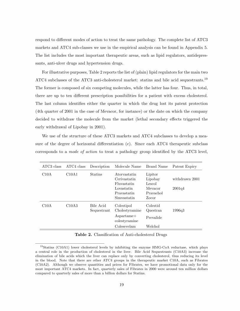
For illustrative purposes, Table 2 reports the list of (plain) lipid regulators for the main two
ATC4 subclasses of the ATC3 anti-cholesterol market: statins and bile acid sequestrants.19
The former is composed of six competing molecules, while the latter has four. Thus, in total,
there are up to ten different prescription possibilities for a patient with excess cholesterol.
The last column identifies either the quarter in which the drug lost its patent protection
(4th quarter of 2001 in the case of Mevacor, for instance) or the date on which the company
decided to withdraw the molecule from the market (lethal secondary effects triggered the
early withdrawal of Lipobay in 2001).
We use of the structure of these ATC3 markets and ATC4 subclasses to develop a mea-
sure of the degree of horizontal differentiation (e). Since each ATC4 therapeutic subclass
corresponds to a mode of action to treat a pathology group identified by the ATC3 level,
ATC3 class ATC4 class Description Molecule Name Brand Name Patent Expiry
C10A C10A1 Statins Atorvastatin LipitorCerivastatin Lipobay withdrawn 2001Fluvastatin LescolLovastatin Mevacor 2001q4Pravastatin PravacholSimvastatin Zocor
C10A C10A3 Bile Acid Colestipol ColestidSequestrant Cholestyramine Questran 1996q3
Aspartame+ Prevalidecolestyramine
Colesevelam Welchol
Table 2. Classification of Anti-cholesterol Drugs
19Statins (C10A1) lower cholesterol levels by inhibiting the enzyme HMG-CoA reductase, which playsa central role in the production of cholesterol in the liver. Bile Acid Sequestrants (C10A3) increase theelimination of bile acids which the liver can replace only by converting cholesterol, thus reducing its levelin the blood. Note that there are other ATC4 groups in the therapeutic market C10A, such as Fibrates(C10A2). Although we observe quantities and prices for Fibrates, we have promotional data only for themost important ATC4 markets. In fact, quarterly sales of Fibrates in 2000 were around ten million dollarscompared to quarterly sales of more than a billion dollars for Statins.
19

we conjecture that the higher the number of ATC4 subclasses in an ATC3 market, the more
differentiation there is.20 We therefore define MoA (for Modes of Action) as the number of
ATC4 subclasses in each ATC3 market, minus 1. That is, for each drug, we identify the
number of rival modes of action to treat the same pathology. We assess whether this variable
appropriately captures horizontal differentiation in the empirical analysis.
Price, Market Share, and Promotion
For each of the drugs included in the selected markets, we compute deflated revenues (R) by
dividing nominal value of sales by the producer price index for the pharmaceutical industry
published by the Bureau of Labor Statistics. Quantities (Q) are reported in standard units
that represent the number of dose units sold for each product; this corresponds to one capsule
or tablet of the smallest dosage or five milliliters of a liquid (i.e., one teaspoon). Standard
units allow comparison across different drug forms and dosages, as all different packages
are subsumed into the same unit of observation. We then compute the average price of a
molecule (P ) by dividing R—i.e., the revenues for all the different packages—by total Q.21
An important feature of our data is that we observe R and Q for two different distribution
channels: hospital (HO) and pharmacies (PH).
Promotional data include three main components: visits to office-based practitioners and
hospital specialists (aka “detailing”); free samples dispensed to physicians (their cost being
estimated as the sales price of the drug); and advertising in professional journals. IMS
Health data on detailing are constructed using a representative panel of physicians who track
their contacts with sales representatives. The amount spent on free samples is based on a
panel of approximately 1200 office staff members in medical practices, while expenditures on
advertising in professional journals are computed by tracking ads placed in approximately
400 medical journals and then adding the publisher’s charge for those ads. The empirical
analysis assumes that promotion to office-based practitioners affects sales in pharmacies,
while promotion to hospital physicians affects the use of drugs in hospitals.
20Dubois and Lasio (2017, Table 6) managed to estimate cross-price elasticities for each pair of moleculesin one ATC3 market. They do report high cross-price elasticities within an ATC4 market, and close to zeroelasticities across ATC4 subclasses.
21This produces a price per standard unit. Note that our empirical specifications control for unobserveddifferences, such as quality and Defined Daily Dose (DDD), across molecules.
20

The promotion level used in the demand specifications reported in Section 5 is computed
with the perpetual inventory method, commonly used for physical capital:
Ait = (1− ρ) Ait−1 + Iit,
where Iit is the quarterly expenditure in promotion retrieved from IMS, and ρ is the quarterly
depreciation rate, assumed to be 0.1 –i.e., about 35% per year.22
Table 3 reports descriptive statistics for these variables, distinguishing between hospitals
and pharmacies. Note that competitors’ promotion refers to the sum of the promotion of all
other drugs in the ATC3 market, each computed according to the equation above. At the
same time, the competitors’ price refers to the average price of all the other molecules in the
market, including generics, and it is computed as the ratio between total revenues and total
quantities in the ATC3 market, after subtracting the revenues and quantities of drug i.
Variables Channel Mean SD Min Max
Hosp 0.117 0.173 0.01 1Market SharesPhar 0.134 0.183 0.01 1
# Competitors Hosp 13.2 8.17 0 46(other Molecules) Phar 12.1 6.62 0 41
Hosp 16.73 70.31 0.02 902.8Own Price
Phar 16.78 71.23 0.05 910.1
Hosp 3269 8101 0 59469Own Promotion
Phar 11165 24592 0 198027
Competitors’ Price Hosp 8.86 28.32 0.02 197.29(average price in ATC3) Phar 4.15 15.19 0.02 122.13
Competitors’ Promotion Hosp 16315 37402 0 231144(total promotion in ATC3) Phar 55871 124654 0 891515
Table 3. Summary Statistics
To get an initial grasp of the differences between hospitals and pharmacies, the upper
part of Table 4 shows that the volume of drugs dispensed in pharmacies is three times as
high as in hospitals. The bottom part reports two different statistics for the drop in volume
market shares following generic entry:23 i) the simple average and ii) the average where each
22All the results reported in Section 5 are robust to setting ρ = 0.3.23The changes are calculated based on the evolution between three years before and after patent expiration.
When patent expiration is close either to the beginning or to the end of the sample period 1994Q1-2003Q4,we take the first (last) available observation for the pre-expiration (post-expiration) period.
21

molecule has been weighted by the advertising intensity of competitors in the same ATC3.
Table 4 suggests that drops in market shares observed after LoE are more pronounced in
pharmacies and in markets in which promotion is more prevalent. We will exploit these
dimensions of heterogeneity in the econometric analysis.
Distribution of QPH/(QPH +QHO)Mean 0.75Median 0.86
Percentage Change before and after Patent Expiration PH HOMarket Shares:Simple Mean -0.31 -0.26Weighted by Drug-A Sales -0.36 -0.25Weighted by ATC3 promotion -0.40 -0.35
Price -0.44 -0.45Advertising -0.89 -0.85
Table 4. Distribution: Pharmacists (PH) & Hospitals (HO)
5 Empirical Analysis
In this section, we first establish whether our theoretical assumptions about the demand side
are confirmed in the data (Section 5.1). We then move to our core contribution, which is to
assess the model’s testable implications regarding market reactions to generic entry (Section
5.2).
5.1 Demand prior to LoE: hospitals and pharmacies
In this subsection, we assess the relative importance of prices and promotion, separately
for the hospital and the pharmacy channel. For this, we estimate the elasticity of a given
branded drug’s market share with respect to its own price and promotion effort, as well as
the cross-elasticities for competing drugs, using an unbalanced panel of active ingredients
until one quarter before LoE.24,25 We also compare these “cross” coefficients between ATC3
24This means that all firms in this subsample face competition only from imperfect substitutes (that canbe generic or branded).
25Note that our aim is not to retrieve price-cost margins, or to carry out merger simulations, for which othermore sophisticated models of differentiated products demand – e.g. Almost Ideal Demand System, nested logit
22

markets made up of either a single or various ATC4 sub-markets.
Anticipating, we find that the elasticity of demand is higher in hospitals. This result is
then used in Section 5.2 to evaluate our first testable implication.
For any ATC market j, equation (7) describes the P3s’ demand for a particular molecule
i at time t. The demand equation is estimated in first-differences in order to remove all
time-invariant, drug-specific fixed effects, such as quality differences:26
∆msi,j,t = α0 + α1 ∆pi,j,t + α2 ∆ai,j,t + α3 ∆p−i,j,t + α4 ∆a−i,j,t
+α5 ∆GENj,t + α6 ∆NCj,t + α7 TEi,j,t + εi,j,t(7)
where ∆msi,j,t , ∆pi,j,t and ∆ai,j,t respectively refer to the change in the logs, i.e., quarterly
growth of quantity market share, price, and promotion effort of branded drug i in ATC3
market j (to repeat, our unbalanced panel includes molecules i until one quarter before
LoE). Similarly, ∆p−i,j,t and ∆a−i,j,t are the competing molecules’ evolution of prices and
promotion in the same ATC3 market (the products in −i may either be branded or generic).
All of these variables are in logarithms, implying that the coefficients can be interpreted as
(short-term) elasticities – see Section 6.3 for a discussion.
To explore whether there are substantial differences between ATC3 markets with a single
or with multiple modes of action, we estimate two cross-price elasticities, α13 and α2+
3 . The
former pertains to ATC3 markets with only one ATC4, while the latter is obtained for ATC3
markets with more than one ATC4. We make the same distinction for competitors’ promotion
(α14 vs. α2+
4 ). This allows us to assess the validity of defining markets at the ATC3 level.
In addition, the estimates of α13 and α2+
3 also shed light on whether MoA is an appropriate
measure of horizontal differentiation.
∆GEN is an indicator variable that takes value 1 in each of the four quarters after the
generization of a competing molecule. This variable captures changes in the competitive
landscape of market j caused by the entry of a new generic competitor. We do not expect it
to be significant: according to our hypotheses, generic entry affects demand only through its
or random coefficient models would be better suited.26Results using FE are qualitatively similar, but we could not identify a set of instruments that simul-
taneously pass the relevant tests for under-identification/weak-identification and the Hansen J test for theexogeneity (orthogonality) of the instruments.
23

effect on prices and promotional effort. Similarly to ∆GEN , the variable ∆NC takes value 1
in the first four quarters after a new competing drug is launched on the market. Finally, the
variable TE (Time to Expiration) counts the number of quarters left to patent expiration,
to account for the impact of the drug’s life cycle on demand.27 In this and all the other
estimations reported in the remainder of this paper, errors have been clustered at the ATC3
level.
The regressors are likely affected by two different problems. The first one is that feedback
from market-share shocks to future prices and advertising may produce endogeneity issues
(reverse causality). The second problem is errors in the measurement of both prices and
promotion effort. The price actually paid may differ from the price we observe in the IMS
database because the latter does not reflect off-invoice ex-post rebates that pharmaceutical
companies grant to large buyers in return for some performance component, such as reaching
a target volume of sales (see Berndt (2012) and footnote 34). Errors in the measurement of
promotion effort stem from the difficulty to observe and quantify monetarily the work of sales
representatives when they visit physicians. Both measurement errors are likely to create an
attenuation bias when estimating (7) using OLS.28
To address these two problems, we instrument prices and promotion expenditure with
three sets of instruments. The first is the number of packages, linear and squared, following
Chaudhuri, Goldberg and Gia (2006). As they argue, the number of packages is related
to the price p because variations in p stem in part from variations in the set of packages
available in each period. An advantage of our dataset over theirs is that we can also control
for promotional effort. The introduction of a new posology or delivery mode is likely to be
accompanied by a resurgence in promotional effort, if only in the form of free samples to
doctors.29 As IMS data on promotion include an estimate of free samples, this instrument
27We use negative values so that the variable is increasing as we approach patent expiration. For instance,-10 and -1 refer, respectively, to ten quarters and one quarter before LoE.
28In the words of Griliches and Hausman (1986), “Errors of measurement will usually bias the first differenceestimators downward (toward zero) by more than they will bias the within estimators.” This problem hasbeen largely discussed in the empirical literature on the estimation of production function (see Griliches andMairesse (1995), among others). It is not by coincidence that the estimation of the demand elasticity topromotion is affected by the same problem of the elasticity of production with respect to capital. In fact,in both cases, econometricians need to construct a measure of “effective stock” looking at data on past andpresent expenditures on physical capital or promotional effort.
29For instance, Ely Lilly started a intense marketing campaign to promote Prozac Weekly, a once-weekly
24

should be highly correlated with promotion expenditures but plausibly uncorrelated with the
measurement error, since the number of packages is measured accurately. The second set
of instruments follows the approach proposed by Dubois and Lasio (2018).30 We use two
variants of their approach. First, we use the residuals of the regression of prices in hospitals
(respectively: pharmacies) over firms’ promotion, molecule dummies and time fixed effects as
an instrument for the pharmacy (resp., hospital) channel. Second, we use the residuals of the
regressions of prices in the United Kingdom over molecule dummies and time fixed effects to
instrument for the corresponding channel in the United States. The third set of instruments
consists of an indicator for the launch of a new product by the same company and a dummy
indicating whether a branded drug has experienced the entry of a generic competitor before
LoE, following a successful “Paragraph IV” challenge.31
This choice of instruments is validated by the Kleibergen-Paap rk-statistic (K-P) for
under-identification, the Angrist-Pischke (A-P) F -test for weak instruments, the Hansen J-
test for the orthogonality conditions, and the C-statistic to test the exogeneity (endogeneity)
of one or more instruments (regressors).32
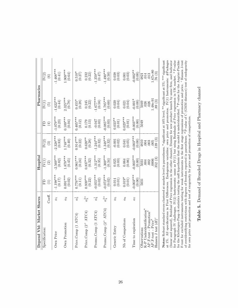
Regression Results
We estimate the empirical model in (7) separately for hospitals and pharmacies in order to
assess whether these two channels react differently to variations in prices and promotion.33
Columns (1) and (4) of Table 5 report the estimates obtained without instrumenting for
formulation of Prozac. Another example is Paxil CR, a controlled-release version of Paxil. Other examplesabound.
30They note that “Controlling for country and time effects, we isolate the quality of each drug proxied bymolecule dummies, which is the part of the price more likely to be correlated with demand unobservables:what remains is supposed to be correlated with the marginal cost of each drug.”
31Paragraph IV of the Hatch-Waxman Act allows generic manufacturers to attempt to enter the marketbefore patent expiration of the original branded drug, either by claiming non-infringement or invalidity ofthe branded product’s patent. A successful Paragraph-IV challenge represents an exogenous shift in thepromotional effort of branded drugs uncorrelated with demand shocks or measurement errors. Branstetter,Chatterjee and Higgins (2011) investigate the welfare effect of accelerated generic entry via Para-IV challengesfor hypertensive drugs.
32Our IV strategy is also supported by the fact that our estimates of price-elasticities are lower but not toofar off the order of magnitude reported by Dubois and Lasio (2017). They use IMS data for France, whereproblems of measurement errors, and the resulting attenuation bias, are less important given the regulatoryconstraints on the pharmaceutical industry.
33Berndt (2002) provides a detailed explanation as to why arbitrage between different channels (here:hospitals and retail pharmacies) cannot occur.
25
Depend
Vbl:
Mark
etShare
sHosp
ital
Pharm
acies
Sp
ecifi
cati
on:
FD
IV(1
)IV
(2)
FD
IV(1
)IV
(2)
Coeff
.(1
)(2
)(3
)(4
)(5
)(6
)
Ow
nP
rice
α1
-1.1
98***
-2.5
69***
-2.3
28***
-1.0
79***
-1.6
22***
-1.4
68***
(0.1
7)
(0.8
2)
(0.8
3)
(0.2
3)
(0.4
4)
(0.4
1)
Ow
nP
rom
oti
on
α2
0.0
91***
1.8
78***
1.7
48***
0.1
09***
2.3
25***
1.9
09***
(0.0
2)
(0.4
5)
(0.4
0)
(0.0
4)
(0.7
8)
(0.6
4)
Pri
ceC
om
p(1
AT
C4)
α1 3
0.7
76***
0.9
61***
0.9
14***
0.4
05***
0.4
55*
0.5
10*
(0.1
1)
(0.2
4)
(0.2
2)
(0.1
2)
(0.2
8)
(0.2
7)
Pri
ceC
om
p(2
+A
TC
4)
α2+
30.9
39***
0.8
37***
0.6
20**
0.1
79
0.2
45
0.2
32
(0.2
2)
(0.3
2)
(0.2
8)
(0.1
3)
(0.2
2)
(0.2
2)
Pro
mo
Com
p(1
AT
C4)
α1 4
-0.0
55***
-1.3
12***
-1.2
44***
-0.0
47
-1.6
77***
-1.3
59***
(0.0
2)
(0.3
5)
(0.3
2)
(0.0
3)
(0.5
8)
(0.4
7)
Pro
mo
Com
p(2
+A
TC
4)
α2+
4-0
.072***
-1.3
69***
-1.3
48***
-0.0
85***
-1.7
85***
-1.4
90***
(0.0
2)
(0.3
4)
(0.3
2)
(0.0
3)
(0.6
0)
(0.5
0)
Gen
eric
Entr
yα
50.0
14
0.0
25
-0.0
01
0.0
33**
0.0
20
0.0
38
(0.0
1)
(0.0
3)
(0.0
2)
(0.0
1)
(0.0
4)
(0.0
3)
Nb
of
Com
pet
itors
α6
0.0
19*
0.0
64
0.0
41
0.0
29***
0.0
21
0.0
01
(0.0
1)
(0.0
6)
(0.0
5)
(0.0
1)
(0.0
4)
(0.0
3)
Tim
eto
expir
ati
on
α7
-0.0
03***
-0.0
03***
-0.0
03***
-0.0
03***
-0.0
01*
-0.0
02**
(0.0
0)
(0.0
0)
(0.0
0)
(0.0
0)
(0.0
0)
(0.0
0)
Obse
rvati
ons
5031
5031
4810
5049
5049
4821
K-P
Under
iden
tifica
tiona
.004
.004
.026
.014
AP
F-t
est
-P
rom
oti
onb
.002
.003
.026
.013
AP
F-t
est
-P
riceb
.0006
.005
1.4
8e-
91
1.6
7e-
80
Hanse
nJ
test
(df)c
.352
(3)
.139
(3)
.89
(3)
.76
(3)
Note
s:R
ob
ust
stan
dard
erro
rscl
ust
ered
at
mark
etle
vel
inp
are
nth
eses
.*
sign
ifica
nt
at
10%
level
;**
sign
ifica
nt
at
5%
;***
sign
ifica
nt
at
1%
.A
llsp
ecifi
cati
on
sin
Fir
stD
iffer
ence
s.E
nd
ogen
ou
svari
ab
les:
ow
np
rice
and
pro
moti
on
.IV
(1)
Inst
rum
ents
:#
Pack
ages
(lin
ear
an
dsq
uare
d),
Res
idu
al
of
Pri
cere
gre
ssio
nin
the
oth
erch
an
nel
,D
um
my
for
new
pro
du
ctla
un
chby
sam
efi
rm,
an
dIn
dic
ato
rfo
rP
ara
gra
ph
IVch
allen
ges
.IV
(2)
Inst
rum
ents
:sa
me
as
IV(1
)b
ut
usi
ng
Res
idu
als
of
Pri
cere
gre
ssio
nin
UK
mark
et.a
P-v
alu
efo
rth
eK
leib
ergen
-Paap
rkst
ati
stic
ste
stin
gth
enu
llhyp
oth
esis
that
the
mod
elis
un
der
iden
tifi
ed.b
P-v
alu
efo
rth
eA
ngri
st-P
isch
ke
F-t
est
for
excl
ud
edin
stru
men
tste
stin
gfo
rw
eak
inst
rum
ents
inth
efi
rst
stage
regre
ssio
ns
of
pro
moti
on
an
dp
rice
.c
Han
sen
J-t
est
of
over
iden
tify
ing
rest
rict
ion
sw
ith
deg
rees
of
free
dom
rep
ort
edin
pare
nth
eses
.d
P-v
alu
eofC
(GM
Md
ista
nce
)te
stof
end
ogen
eity
for
ow
np
rice
an
dp
rom
oti
on
an
dte
stof
exogen
eity
for
pri
cean
dp
rom
oti
on
of
com
pet
itors
.
Tab
le5.
Dem
and
ofB
ran
ded
Dru
gsin
Hos
pit
alan
dP
har
mac
ych
ann
el
26

prices and promotion. Comparing these results with those in Columns (2 and 3) and (4
and 5) confirms the existence of an attenuation bias due to errors in measuring prices and
promotion intensity. They also reveal price and promotion elasticities that are in the upper
range of those found in the literature (but see footnote 32). Section 6.3 explains why these
elasticities ought to appropriately capture the effects of price and promotion movements
associated with generic entry.
A number of findings emerge from the IV results. First, the estimated elasticity w.r.t.
own-price is higher in hospitals than in pharmacies. Second, the coefficients pertaining to the
price of competitors (Price Comp), α13 and α2+
3 , are significantly larger and more precisely
estimated in the hospital channel. Third, for pharmacies, only α13 is significant (and at
the 10% level). Overall, these findings reinforce the message that hospitals are more price-
sensitive than private practice doctors.
This difference is in line with Inderst and Ottaviani (2012)’s intuition: private practice
doctors do not directly benefit when patients buy a cheaper alternative (possibly, they even
lose some perks offered by pharmaceutical companies) and, at the same time, these patients
only pay a fraction of the drug’s price, thanks to third-party payer coverage. By contrast,
hospitals are residual claimants: their margin depends one-for-one on procuring drugs at a
discount since they then charge the patient a pre-determined reference price.34
Fourth, we find that the elasticities for own- and cross-promotion are of the right sign,
large, and precisely estimated in both channels. When instrumented, the point estimates
increase substantially, confirming the extent to which this variable is affected by endogeneity
problems. Interestingly enough, the two coefficients α14 and α2+
4 are similar both within and
between channels.
Fifth, the overall picture that emerges from the above results is that the ATC3 level
appropriately represents a molecule’s market even if price competition appears more subdued
across ATC4 sub-classes. The latter observation suggests that coexistence of different modes
of action within a market should be a good proxy for horizontal differentiation.
34 This is also in line with the patterns evidenced by Berndt (2002, p60): “Next lowest are prices to hospitalsfor inpatient prescription use only [...] [P]rices charged retail pharmacies for their cash-paying customers arediscounted off “list” price the least”.
27

The coefficients on the headcount of genericized molecules and on the number of competi-
tors are statistically insignificant once we properly control for endogeneity. These results con-
firm the working assumptions made in our model: (a) generic entry affects demand through
the price and promotion of a given molecule. (b) Market share movements of incumbents are
not driven by the launch of new molecules above and beyond the latter’s effects on price and
promotion.
5.2 The effects of generic entry (testable implications 1-3)
The previous section produced three results that are important to test the predictions of the
model. First, the ATC3 level is a reasonable definition of a therapeutic market. Second, the
variable MoA (modes of action, see p20) qualifies as a proxy for horizontal differentiation
within a market. Third, hospitals are comparatively more price sensitive than pharmacies. In
addition, we can control for other time-invariant differences (such as vertical differentiation)
through molecule fixed effects.
Adding a variable to capture market size, we have all the elements needed to evaluate
testable implications 1-3:
yi,j,c,t = γ1GENj,t + γ2Hosp GENj,t + γ3MoAt GENj,t (8)
+γ4Smalli GENj,t + ρ yi,j,c,t−4 + β′Xi,j,c,t + αi + εi,j,c,t,
where yi,j,c,t ∈ {ms, a, p} is the log of either the market share, promotion level, or price, of the
patent-protected drug i in ATC3 market j sold in channel c ∈ {Hospital, Pharmacy}, at time
t. GENj,t counts the number of molecules that lost exclusivity in the same market. Hosp is a
dummy for the hospital channel, and MoAt is our proxy for horizontal differentiation. To test
for the effect of market size (testable implication 3), we distinguish between a “blockbuster”
group, defined as the set of the top 25% selling drugs during the entire time period, and the
remaining 75%, which we identify with the indicator variable Smalli.
To check the robustness of our results, we also rely on an alternative count measure of
generic entries, by discarding the LoE events that concerned low-selling products. More
precisely, we only count the LoEs of the 20 drugs (out of 95) with the largest average sales
28

over the sample period. We will refer to this variable as GEN IMP , for IMPortant generic
entries.
Equation (8) also includes the one-year lag of the dependent variable (i.e., four quarters)
to capture dynamic autoregressive processes, such as possible seasonal variations in drug
usage over the year (e.g. antibiotics and antihistamines). The set of control variables X
includes the number of competing molecules to proxy the intensity of competition, time to
expiration, and a complete set of time dummies. As for other specifications, the data for y
pertain to branded drugs until one quarter before patent expiration.
According to testable implication 1, following the LoE of some molecule A, the market
share of an on-patent molecule B should increase less (or decrease more) if δ is higher. In
light of the results of Section 5.1, that elasticity is higher in hospitals. We thus expect γ2 to
be negative. According to testable implication 2, we expect γ3 to be negative: the market
share of molecule B should increase less (or decrease more) if the ATC3 market features
more horizontal differentiation. Finally, testable implication 3 predicts that γ4 should
be negative: on-patent drug B should be more likely to lose market share if the revenue it
generated is small prior to LoE.
Column 1 and 2 of Table 6 reports the FE estimates with market share as the dependent
variable. All the coefficients have the expected signs and they are all significant at 5% level,
with the exception of γ2 in column 1. The coefficients in column (2) show that, when we
restrict the analysis to the most important cases of generic entry, there is a substantial
increase in the magnitude of the point estimates, and γ2 also becomes significant at the 5%
level. Yet, the relative magnitude of the coefficients remains similar. Overall, these estimates
are consistent with our testable implications. First, we observe mainly instances of branded
drugs increasing their volume market share following the genericization of a competitor:
γ1 is positive and significant. As we detail in Section 6.3, the impact of generic entry on
promotional effort and prices is an important factor to explain this evolution.
Second, and in line with testable implication 1, the higher elasticity of demand in the
hospital channel reduces the market share gain by a quarter for the drugs remaining on
patent: in column (2), the coefficient on HOSP ∗ GEN is negative, significant, and equal
to a fourth of γ1. In line with testable implication 2, the negative coefficient γ3 confirms
29

En
dog
enou
sva
riab
le:
ms
ms
(GENIMP
)m
sm
s(GENIMP
)P
RO
MP
RIC
E(F
E)
(FE
)(G
MM
)(G
MM
)(F
E)
(FE
)
Coeff
.(1
)(2
)(3
)(4
)(5
)(6
)
GE
Nγ1
0.1
74***
0.3
20***
0.1
45***
0.2
89***
0.3
57***
0.0
54
(0.0
4)
(0.0
9)
(0.0
4)
(0.0
7)
(0.1
4)
(0.3
1)
Hos
p*G
EN
γ2
-0.0
23
-0.0
81**
-0.0
36**
-0.1
10***
-0.0
38
0.0
67
(0.0
2)
(0.0
3)
(0.0
2)
(0.0
3)
(0.0
3)
(0.1
2)
MoA
*GE
Nγ3
-0.0
41***
-0.0
77***
-0.0
44***
-0.0
87***
-0.0
97**
-0.2
01
(0.0
1)
(0.0
3)
(0.0
1)
(0.0
3)
(0.0
4)
(0.1
7)
Sm
all*
GE
Nγ4
-0.1
06***
-0.2
34***
-0.0
77**
-0.1
97***
-0.3
90***
0.0
41
(0.0
4)
(0.0
7)
(0.0
4)
(0.0
6)
(0.1
2)
(0.4
7)
Tim
eto
Exp
irat
ion
-0.0
16***
-0.0
14***
-0.0
18***
-0.0
17***
-0.0
24**
0.1
20*
(0.0
0)
(0.0
0)
(0.0
0)
(0.0
0)
(0.0
1)
(0.0
7)
Nu
mb
erof
Com
pet
itor
s-0
.006
-0.0
07
-0.0
07
-0.0
08
-0.0
17
0.3
66
(0.0
2)
(0.0
2)
(0.0
1)
(0.0
1)
(0.0
4)
(0.2
4)
Lag
ged
dep
.va
r.ρ
0.5
51***
0.5
54***
0.7
04***
0.7
30***
0.0
42
0.5
69***
(0.0
4)
(0.0
4)
(0.1
0)
(0.1
0)
(0.0
4)
(0.2
0)
Ob
serv
atio
ns
9041
9041
8622
8622
9041
9041
Han
sen
J-t
est
(df)a
0.2
53
(69)
0.3
23
(69)
AR
1 p0.6
77
0.6
73
AR
2 p0.2
10
0.1
78
Note
s:R
ob
ust
stan
dard
erro
rscl
ust
ered
at
AT
C3-m
ark
etle
vel
inp
are
nth
eses
.*si
gn
ifica
nt
at
10%
level
;**si
gn
ifica
nt
at
5%
;***si
gnifi
cant
at
1%
.E
nd
ogen
ou
svari
ab
le:
lagged
dep
end
ent
vb
lon
eyea
rb
efore
.In
stru
men
t:la
gs
of
nu
mb
erof
com
pet
itors
an
dm
ark
etco
nce
ntr
ati
on
.a
P-v
alu
eof
Han
sen
J-t
est
of
over
iden
tify
ing
rest
rict
ion
sw
ith
deg
rees
of
free
dom
rep
ort
edin
pare
nth
eses
Tab
le6.
Eff
ect
ofa
com
pet
itor
’sge
ner
iciz
atio
non
on-p
aten
td
rugs
30

that markets characterized by higher horizontal differentiation experience a smaller increase
in market share. The interaction between the revenue size indicator variable and the generic
count (γ4) is also significant and of the expected sign, confirming testable implication 3.
Our testable implications should also apply to promotion and prices. The results are
presented in columns 5 and 6: we find that promotion reacts in the same way as market shares,
although by a larger magnitude. By contrast, the coefficients for prices are not significant.
This reinforces the overall message that promotion is the privileged mode of competitive
interactions, while it may be more difficult to increase prices—which have probably been
previously negotiated with third party payers—each time a generic enters the market.35
Because of the presence of the lagged dependent variable, the use of fixed effects leads
to a downward bias (known as “Nickell bias”) in the point estimate of ρ, which can be
transmitted to the other coefficients. Although this bias is small in dataset with large T . We
check the robustness of our results given the unbalanced nature of our dataset. To this end,
we use the GMM estimator with the forward orthogonal deviation (FOD) transformation
proposed by Arellano and Bover (1995). An important advantage of FOD is that, unlike the
First-Difference estimator which introduces a moving average structure in the error term,
the lack of correlation in the transformed errors is preserved if the original ones are not
autocorrelated. The instruments we use are composed of lags of the number of competitors
and the Herfindahl-Hirschman concentration index.36 Because the number of instruments
generated by our GMM framework is quadratic in T , we avoid the problem of using “too
many weak instruments” by using the collapse option as explained in Roodman (2006). The
statistical tests reported at the end of Table 6 support our IV strategy. As expected, the
coefficient on the lagged dependent variables in columns (3) and (4) is now higher. Overall,
the IV approach confirms and reinforces the FE results, without affecting the magnitude of
the other coefficients.
35Moreover, as emphasized on p.24, we cannot observe price rebates, which probably are the easiest-to-usemargin of adjustment for actual sale prices.
36For each specification, we also experimented with additional lags of the dependent variable. While theresults were qualitatively similar, the Hansen test was often not passed.
31

6 Robustness and sensitivity
This section addresses three issues. First, we check whether our results are robust to ever-
greening strategies. We do this by reestimating our demand equation (7) excluding instances
of LoE experienced by a drug whose originator also owned a second-generation product in
the same market. We also reestimate equation (8) to check whether evergreening amplifies
the migration to on-patent drugs. Second, we investigate the stability of the coefficients of
the demand equation to changes in the set of instruments. Finally, we assess whether the
elasticities reported in Table 5 do a good job in predicting observed post LoE developments.
In addition, we compare these estimates with those typically found in the literature.
6.1 Evergreening
As detailed in Section 2, “evergreening” refers to the introduction of second-generation ver-
sions of the drugs by the very firm that faces the loss of exclusivity on a drug. The European
Commission’s Pharmaceutical Sector Inquiry identified a related tactic, which is to withdraw
the first-generation product soon after the launch of the second generation product and before
LoE for the first generation product (SI, p.365).
One may argue that this is the main rationale for the reduction in market shares of
the molecules losing exclusivity, instead of generic competition. We instead contend that
evergreening is just an instance in which the firm losing exclusivity and the one proposing
a branded substitute are the same. The logic of organizing the transfer of patients via an
intense promotion campaign is the same; the confluence of interests should only make the
effects stronger. Hence, the mechanism we document is not incompatible with evergreening.
On the contrary, the rationale underpinning evergreening strategies requires that promotion
be effective.37
In our dataset, we observe twenty cases where the originator facing generic entry also
37One originator (EC Sector Inquiry, p.360, #1028) reported: “This means each patient that is not switchedquickly enough to [our second generation product] is forever lost to the generics. Once the patient is switchedto [our second generation product] the physician does not have to, cannot and will not switch him to a generic,and what is more important: the pharmacist cannot substitute!” Figure 138, p. 361 of the SI indicates thatmost second generation launches occur prior to the first generation product experiencing LoE.
32

Depend Vbl: Market Shares Hospital Pharmacies
Specification: FD FD-IV FD FD-IVCoeff. (1) (2) (3) (4)
Own Price α1 -1.156*** -2.080*** -1.082*** -1.864***(0.17) (0.77) (0.24) (0.55)
Own promotion α2 0.091*** 1.542*** 0.099** 1.830***(0.03) (0.39) (0.04) (0.60)
Price Comp (1 ATC4) α13 0.757*** 0.898*** 0.421** 0.534*
(0.12) (0.22) (0.12) (0.29)
Price Comp (2+ ATC4) α2+3 1.003*** 0.608** 0.212 0.264
(0.25) (0.30) (0.14) (0.22)
Promo Comp (1 ATC4) α14 -0.062*** -1.116*** -0.035 -1.270***
(0.02) (0.33) (0.04) (0.45)
Promo Comp (2+ ATC4) α2+4 -0.071*** -1.171*** -0.076** -1.387***
(0.02) (0.31) (0.03) (0.46)
Generic Entry α5 0.010 -0.001 0.030** 0.028(0.01) (0.02) (0.01) (0.03)
Nmb of Competitors α6 0.020* 0.022 0.031*** 0.005(0.01) (0.05) (0.01) (0.03)
Time to Expiration -0.003*** -0.003*** -0.003*** -0.002**(0.00) (0.00) (0.00) (0.00)
Observations 4556 4335 4576 4348K-P Underidentificationa .0077 .0397AP F-test - Promotionb .0053 .0348AP F-test - Priceb .0083 .0001Hansen J test (df)c .253(3) .583(3)
Notes: Robust standard errors clustered at market level in parentheses. * significant at 10% level;** significant at 5%; *** significant at 1%. All specifications in First Differences. Endogenous vari-ables: Own price and promotion. IV Instruments: #Packages (linear and squared), Residual of Priceregression in UK market, Dummy for new product launch by same firm, and Indicator for ParagraphIV challenges. a P-value for the Kleibergen-Paap rk statistics testing the null hypothesis that themodel is underidentified. b P-value for the Angrist-Pischke F-test for excluded instruments testing forweak instruments in the first stage regressions of promotion and price. c Hansen J-test of overiden-tifying restrictions with degrees of freedom reported in parentheses. d P-value of C (GMM distance)test of endogeneity for own price and promotion and test of exogeneity for price and promotion ofcompetitors.
Table 5b. Demand for Branded Drugs:Sample Excluding Evergreening Episodes
33

owns one or more on-patent drugs in the same ATC3 market.38 To assess the validity of our
argument, we re-estimate equation (8) excluding the episodes of generic entry in which the
firm that experiences the LoE episode also owned marketing rights for another drug in the
same ATC3. This shrinks our sample size by about 10%, which reduces the significance of
some coefficients.
The results are presented in Table 5b: in comparison with Table 5, the coefficients on
own and competitors’ promotion remain largely unchanged. This provides strong support to
the idea that ever-greening is not the whole story behind the market share loss of molecules
losing exclusivity.
In Table 6b, we re-estimate specifications (1) and (3) in Table 6, which use market shares
FE GMMCoef. (1) (2)
GENNEverG γ1NEG 0.163*** 0.138***(0.04) (0.04)
GENEverG γ1EG 0.272*** 0.234***(0.07) (0.06)
Hosp ∗GEN γ2 -0.020 -0.033*(0.02) (0.02)
MoA ∗GEN γ3 -0.040*** -0.043***(0.01) (0.01)
Small ∗GEN γ4 -0.111*** -0.084**(0.04) (0.04)
Time to expiry -0.017*** -0.018***(0.00) (0.00)
# competitors -0.008 -0.008(0.02) (0.01)
Lagged mkt share ρ 0.550*** 0.690***(0.04) (0.10)
Obs 9041 8622Hansen p-value (df) 0.20 (69)AR1p 0.673AR2p 0.240
Notes: Robust std errors clustered at ATC3-market level in parentheses. *sig-nificant at 10% level; **significant at 5%; ***significant at 1%. Endogenousvariable: lagged dependent vbl 1 year before. Instruments: lags of # competitorsand market concentration.
Table 6b. Effect of evergreening on on-patent drugs
38These include the following two well-know cases: (i) Mevacor (Lovastatin), whose patent expired in 2001,and the follow-on statin Zocor (Simvastatin), both produced by Merck and (ii) Losec (Omeprazole), whosepatent expired in 2002, and Nexium (Esomeprazol), both owned by AstraZeneca
34

as the dependent variable. The difference with Table 6 is that we now distinguish between
those instances in which the molecule that loses exclusivity is owned by a company that has
another drug in the same ATC3. That is, GENEverG refers to generic entry in markets where
the firm losing exclusivity had the opportunity to rely on an evergreening strategy, whereas
GENNEverG refers to the other instances of LoE. In line with our conjecture, we find that
the coefficient on GENEverG is much larger than the coefficient on GENNEverG.
6.2 Instruments and Robustness of Demand Elasticities
Here, we discuss two potential concerns about our IV strategy: (1) the residuals of the first-
stage regression of prices in the other channel or UK prices as dependent variables, may not
be orthogonal to firm-wide demand shocks. (2) The results in Table 5 may look stable only
because our instruments are highly correlated with each other. To address such concerns
and shed additional light on the adequateness of our identification strategy, we repeat the
analysis of Table 5, but with a reduced set of instruments.39
Table 5c reports results where we drop: (i) the residuals of the price regression (columns
1); (ii) the number of packages (columns 2); and (iii) the indicator for the introduction of a
new product (columns 3).
The specification in column (1) of Table 5c drops the instruments that could potentially be
correlated with firm-wide demand shocks (e.g. in the unlikely case that price variations in the
UK are contemporaneously correlated with demand shocks in the US). We find that the results
for the hospital channel are extremely stable. Not surprisingly, the fact that we drop the two
instruments that are more relevant for prices produces less precise estimates for own-price
elasticity in the pharmacy channel. Yet, all the other coefficients are essentially unaffected.
The test for under-identification confirms that we have a weak instruments problem in the
first-stage regression for prices; hence the choice of instruments used to obtain the results
reported in Table 5.
Next, in Section 5.1, we claimed that the number of packages is particularly important
to identify the elasticity of demand w.r.t. promotion. To check that this is indeed the case,
39We thank two anonymous referees for their suggestions. Also, note that a previous version of this paperused average price in other markets (so called “Hausman-type” instruments), which produced similar results.
35

Depend
Vbl:
Mark
etShare
sHosp
ital
Pharm
acies
Sp
ecifi
cati
on:
(1)
(2)
(3)
(1)
(2)
(3)
Coeff
.
Ow
nP
rice
α1
-2.6
38*
-2.2
93***
-2.9
38***
-7.4
27
-1.4
44***
-1.6
21***
(1.5
4)
(0.7
5)
(1.0
1)
(8.0
3)
(0.4
0)
(0.4
4)
Ow
nP
rom
oti
on
α2
2.0
11***
1.1
51***
2.2
30***
2.1
57***
1.7
85*
2.3
20***
(0.4
9)
(0.3
1)
(0.6
0)
(0.7
8)
(0.9
4)
(0.7
9)
Pri
ceC
om
p(1
AT
C4)
α1 3
0.9
49***
0.9
31***
1.0
88***
0.6
41*
0.5
09**
0.4
55*
(0.2
5)
(0.1
6)
(0.3
0)
(0.3
8)
(0.2
4)
(0.2
8)
Pri
ceC
om
p(2
+A
TC
4)
α2+
30.8
34**
0.7
03***
0.6
66*
0.1
43
0.2
23
0.2
45
(0.3
4)
(0.2
2)
(0.4
0)
(0.2
4)
(0.2
1)
(0.2
2)
Pro
mo
Com
p(1
AT
C4)
α1 4
-1.4
03***
-0.7
70***
-1.4
71***
-1.5
22**
-1.2
54*
-1.6
73***
(0.3
8)
(0.2
5)
(0.4
4)
(0.6
0)
(0.7
2)
(0.5
9)
Pro
mo
Com
p(2
+A
TC
4)
α2+
4-1
.466***
-0.8
98***
-1.6
42***
-1.6
50***
-1.3
82*
-1.7
80***
(0.3
6)
(0.2
4)
(0.4
5)
(0.6
0)
(0.7
3)
(0.6
1)
Gen
eric
Entr
yα
50.0
20
0.0
03
0.0
20
0.0
08
0.0
38
0.0
20
(0.0
3)
(0.0
1)
(0.0
3)
(0.0
4)
(0.0
3)
(0.0
4)
Nb
of
Com
pet
itors
α6
0.0
67
0.0
37
0.0
64
0.0
23
0.0
06
0.0
21
(0.0
6)
(0.0
3)
(0.0
7)
(0.0
3)
(0.0
3)
(0.0
4)
Tim
eto
expir
ati
on
α7
-0.0
03***
-0.0
03***
-0.0
03***
-0.0
01
-0.0
02**
-0.0
01*
(0.0
0)
(0.0
0)
(0.0
0)
(0.0
0)
(0.0
0)
(0.0
0)
Obse
rvati
ons
5057
4810
5031
5049
4821
5049
K-P
Under
iden
tifica
tiona
.0075
.0075
.0042
.4206
.1679
.0154
AP
F-t
est
-P
rom
oti
onb
.0009
.0067
.0033
.0285
.1381
.0165
AP
F-t
est
-P
riceb
.0186
.0283
.0003
.4500
<0.0
01
<0.0
01
Hanse
nJ
test
(df)c
.211
(2)
.608
(2)
.775
(2)
.952
(2)
.760
(2)
.736
(2)
Note
s:R
ob
ust
stan
dard
erro
rscl
ust
ered
at
mark
etle
vel
inp
are
nth
eses
.*si
gn
ifica
nt
at
10%
level
;**si
gn
ifica
nt
at
5%
;***si
gn
ifica
nt
at
1%
.A
llsp
ecifi
cati
on
sin
Fir
stD
iffer
ence
s.E
nd
ogen
ou
svari
ab
les:
ow
np
rice
an
dp
rom
oti
on
.In
stru
men
ts:
inco
lum
n(1
):#
Pack
ages
(lin
ear
an
dsq
uare
d);
Du
mm
yfo
rN
ewP
rod
uct
lau
nch
;an
dIn
dic
ato
rof
“P
ara
gra
ph
IV”
chall
enge;
inco
lum
n(2
):R
esid
ual
of
Pri
cere
gre
ssio
nin
oth
erC
han
nel
;R
esid
ual
of
Pri
cere
gre
ssio
nin
UK
;D
um
my
for
New
Pro
du
ct;
an
dIn
dic
ato
rfo
r“P
ara
gra
ph
IV”
challen
ge;
inco
lum
n(3
):#
Pack
ages
(lin
ear
an
dsq
uare
d);
Res
idual
of
Pri
cere
gre
ssio
nin
oth
erC
han
nel
;an
dIn
dic
ato
rfo
r“P
ara
gra
ph
IV”
challen
ge.
Tab
le5c.
Dem
and
ofB
ran
ded
Dru
gsin
Hos
pit
alan
dP
har
mac
ych
ann
els
36

column (2) in Table 5c drops this variable from the set of instruments. In line with our
conjecture on identification, we find that the price elasticities are largely unchanged, while
the point estimates for promotion are lower in both channels and less precisely estimated
in the case of pharmacies. Having dropped our instrument of choice for promotion, the
AP F-test for promotion fails in the pharmacy channel; which lends further support to our
IV strategy in Table 5. In addition, these results are in line with the conjecture that the
pharmacy channel is more sensitive to promotion.
Finally, column (3) drops the indicator for new product launches from the instrument set.
The results barely change, although a couple of coefficients are less precisely estimated. This
indicates that the information content of this instrument is worth exploiting in the context of
our IV strategy. Very similar results (not reported) are obtained when dropping the indicator
for Paragraph IV challenges.
Thus, overall, the additional set of results reported in Table 5c tend to confirm the
robustness of our findings, and support our initial choice of instruments. In particular,
removing instruments results in under-identification tests that fail, and coefficients on the
variables associated to the particular instrument that are less precisely estimated.
6.3 Assessing demand elasticities: an out-of-sample exercise
Our estimates for promotion and, to a much lesser extent, price elasticities are in the upper
range of what is found in the literature that uses U.S. data, but are not uncommon (see e.g.
Narayanan et al. (2005) or Lakdawalla and Philipson (2012, Table 4); see also footnote 32).
We conjecture that there are three main reasons for this: 1) Like Lakdawalla and Philipson
(2012) or Dubois and Lasio (2018), our sample covers a long period and includes a large
number of LoE events. Patent expiration represents a significant (exogenous) shock that
produces a larger-than-usual variation in price and promotional effort. In the presence of
switching costs, these are likely to trigger more substantial changes in prescription behavior
than temporary or small variations.40 2) We control for both own- and cross-price and
40Switching costs include for instance having to study the properties of alternative drugs and convincingpatients to try them out. Klemperer (1987) shows that even small switching costs can be sufficient for firmsto reach fully collusive pricing behavior. Generic entry, in contrast, produces a significant price change, whichhas the potential to induce a switch. Interestingly, the aforementioned studies of Lakdawalla and Philipson
37

promotion effects, which addresses a potential omitted-variable bias due to the arms-race
nature of promotion. Note that, if the slope of the promotion reaction function is close to 1
(the actual correlation between own and competitor promotion is above 0.6), then the sum of
own and cross promotion elasticity yields a figure very close to what is typically reported in the
literature. In that respect, it is worth noting that promotion elasticities are typically obtained
without including competitors’ promotion in the analysis (e.g. Mizik and Jacobson 2004). 3)
We use a rich set of instrumental variables: our initial estimates in columns (1) and (4)
display significantly lower estimates for promotion elasticities (possibly due to measurement
errors in promotion efforts). Moreover, around one third of the drugs in our sample are
not actively promoted on the basis of IMS data, which may also contribute to biasing the
estimates towards zero. Our instruments appear to address these issues satisfactorily.
Regarding (own) price elasticities, we note that the findings of an elasticity below 1 are
difficult to reconcile with profit maximization. By contrast, our point estimates in Table 5,
Columns (2) and (5), are compatible with price-cost margins in the 40-55% range. This order
of magnitude is in line with the price reductions observed following generic entry, and it is
also close to the results reported by Rizzo (1999), and more recently, by Narayanan et al.
(2005). More precisely, the latter report (p.286) own-price elasticities ranging from 2.18 to
2.61 for three antihistaminics.41
With regard to promotion elasticities, the meta-analysis by Kremer et al. (2008) reports
that estimates ranging from a negative value (Venkataraman and Stremersch 2007) and 1.39
(Berndt, Pindyck and Azoulay 2003), and the average of all estimates is 0.35. More recently,
Dave and Saffer (2012, Table 2) report an elasticity w.r.t. detailing comprised between 0.44
and 0.52. While such elasticities are certainly accurate to describe how prescription behavior
reacts to marginal changes in promotion effort (e.g. comparing a doctor who received two
visits per month with another who received only one), we argue that they may not appropri-
ately capture the effects of a sustained, nation-wide, promotional effort to influence doctors’
(2012, Table 4) and Dubois and Lasio (2017, Table 4) also capture substantial reactions, which differ fromother studies that focus on, say, short-term and minor shocks that are doctor-specific (see e.g. Shapiro 2016).Note that their and our estimates are consistent with each other, despite substantially different estimationstrategies, and data coverage.
41The elasticities reported by Dubois and Lasio (2017, Table 4) are much higher and range from values of4.06 for the U.S. and 5.5 for Germany.
38

prescription behavior over the long haul.
Formally, we check whether the promotion elasticities reported in the literature can be
made consistent with the observed shift in prescription behavior post-LoE. The evolution of
a molecule’s sales (or market share when total market size is normalized) must be such that:
∆Q
Q' ηP ·
∆P
P+ ηA ·
∆A
A,
where ηP is the price elasticity, and ηA the advertising elasticity.
Table 4 indicates that generic entry produces an average price drop of about 44-45%
depending on the channel, and an average drop in the flow of promotion between 85 and
90%. We calculate that, once converted into stocks, these correspond to a drop of respectively
69.4% and 72.9% three years after LoE. Taking the pharmacy channel as an example, the
predicted change in the market share of the now generic molecule should thus be:
∆Q
Q' ηP · (−0.45) + ηA · (−0.694) .
If we take a lower reasonable bound of ηP = 1, and use the estimates for ηA reported in
the meta-analysis by Kremer et al. (2008), it turns out that 55 of the 58 reported elasticities
are incompatible with any drop in the molecule’s market share, and therefore with actual
observations. The same applies for the elasticities reported in Dave and Saffer (2012, Table
2, column 7).
If instead we use our IV-regression results from Table 5, we find that, in hospitals, the
predicted change in market share is: −2.328 · (−0.45) + 1.748 · (−0.694) = −0.17, which
compares to an actual average drop of about −0.26 (see Table 4). Following the same proce-
dure for pharmacies, the predicted evolution is: −1.468 · (−0.44) + 1.909 · (−0.729) = −0.67
(actual average drop about −0.31).42 Thus, regression results in Table 5 predict (i) a drop
in market shares for both segments and (ii) a larger drop for pharmacies. Note that the
predicted drop in pharmacies is substantially larger than observed levels. This is compatible
with the third party payers’ active promotion of generics use.
Beyond this technical point, it should be recalled that the large pharmaceutical corporates
42With the coefficients of columns 2 and 5, the predicted drops are -0.15 and -0.88.
39
spend 15-20% of their revenue on promotion in various forms. If detailing were not effective,
it would be hard to rationalize such spending by well established and sophisticated firms.
Their behavior can only be compatible with profit maximization if advertising elasticities
are north of 0.2 in the case of constant returns to promotional effort, or significantly higher
in the presence of steeply increasing marginal cost of detailing (MC � AC). Berndt et al.
2003), and Manchanda, Rossi and Chintagunta (2004) provide convincing evidence of such
fast decreasing returns to detailing, and Chressanthis et al. (2014) document that detailing
agents face increasing difficulties to access physicians.
7 Conclusions and Welfare Implications
This paper analyzes the consequences of generic entry on on-patent drugs. Our research ques-
tion was prompted by the puzzling observation that intense intra-molecular price competition
following generic entry typically does not lead to increased volume sales for the molecule that
experiences Loss of Exclusivity (LoE). We posit that what drives the aforementioned outcome
is the importance of detailing and other forms of promotion combined with an asymmetry in
the competitive shock associated with generic entry. Our model shows that a product selling
at much reduced price-cost margins may end up selling less, simply because the firm hit by
stiffer competition largely stops promoting its product.
This phenomenon helps explain why, despite generics accounting for 75-90% of the market
for the molecules that have lost exclusivity, their overall effect on the market has fallen short
of expectations. Legislators and purchasers on both sides of the Atlantic have had to actively
promote generic penetration, and yet expenditures on drugs kept on rising.
Our model identifies the circumstances under which the molecule facing generic entry
should experience a market share drop. This is when the market is large, the price elasticity
of demand is low and, strikingly, when horizontal product differentiation is limited. These
theoretical predictions are confirmed by our empirical analysis.
Going one step further, the model allows us to make some inferences regarding allocative
efficiency and patient/consumer surplus. Following the logic in Inderst and Ottaviani (2012),
our model reckons that promotion does influence physicians’ prescription behavior, even when
40

it does not directly enter patients’ utility. We find that a sufficient condition for patient
(consumer) surplus to increase after generic entry is that the market share of molecules
remaining on patent decreases in equilibrium (the price and promotion then falls for both
molecules). As we saw, this condition is rarely met in practice, meaning that asymmetric
competition typically hurts patients according to that definition of surplus. The model also
allows us to assess when the change in market shares produced by generic entry brings the
market allocation closer to the first best. The answer is never, and a ban on promotion would
not solve the problem (Proposition 5 in Appendix 4).
As we argued in the introduction, these mechanisms are still poorly understood today.
Yet, regulation and market interventions did evolve since the early 2000s. In recent years,
US Third Party Payers (TPPs) started providing increasingly high-powered incentives to
promote generic use. For instance, it is now common for insured patients to face higher co-
payments for on-patent drugs when generics are available. In Europe, generic use has been
encouraged by social security systems, with varying degrees of success.
Our model and empirical results provide a rationale for the extent of TPP activism
over the last two decades: it is an endogenous response to the strategies implemented by
originators. We show that generic entry alone is typically insufficient to contain expenditure
in large and profitable therapeutic markets. Hence, additional incentives and constraints on
prescription behavior are necessary to actually deliver savings.
Still, the extent to which the prescribing behavior by some private practice physicians can
be made responsive to these efforts is an open question. Moreover, we note that in the case of
biologics, TPPs activism is bound to be much less effective, as bio-similars are not considered
as direct substitutes. Under these circumstances, doctors’ discretionary choices will remain
central. It is not unreasonable to think that detailing and other types of corporate spending
directed at the medical profession will continue to be a key determinant of prescription
behavior.
41

References
Aitken, M., L., Berndt, E. R., and Cutler, D., M. (2009). “Prescription Drug SpendingTrends In The United States: Looking Beyond The Turning Point”, Health Affairs 28, no.1:w151-w160
Aitken, M., L., Berndt, E. R., Bosworth, B., Cockburn I. M., Frank, R., Klein-rock, M. and Shapiro, B. (2013). “The Regulation of Prescription Drug Competitionand Market Responses: Patterns in Prices and Sales Following Loss of Exclusivity”. NBERWorking Paper 19487.
Apple (2013). UNITED STATES SECURITIES AND EXCHANGE COMMISSION,Form 10-K, September 28. http://investor.apple.com/secfiling.cfm?filingid=1193125-13-416534&cik=#D590790D10K HTM TOC590790 1
Arellano, M. and Bover, O. (1995). “Another look at the instrumental-variable estimationof error-components models”. Journal of Econometrics, 68, pp. 29–52
Berndt, E.R. (2002). “Pharmaceuticals in U.S. Health Care: Determinants of Quantityand Price”. Journal of Economic Perspectives, Vol. 16(4), pp. 45–66.
Berndt, E.R. and Dubois P. (2016). “Impacts of Patent Expiry of Pharmaceutical Treat-ments in Eight OECD Countries, 2004-2010”. International Journal of the Economics ofBusiness, vol. 23(2):125–147.
Berndt, E.R., Kyle, M., and Ling, D. (2003). “The Long Shadow of Patent Expiration:Generic Entry and Rx-to-OTC Switches,” in Scanner Data and Price Indexes, ed. R. Feenstraand M. Shapiro University of Chicago Press, pp. 229–267
Berndt, E.R., Pindyck, R and Azoulay, P. (2003) “Consumption Externalities and Dif-fusion in Pharmaceutical Markets: Antiulcer Drugs”. The Journal of Industrial Economics,vol. 51(2): 243-270.
Branstetter, L.G., Chatterjee C. and Higgins M.J. (2011). “Regulation and Welfare:Evidence from Paragraph IV Generic Entry in the Pharmaceutical Industry”. NBER WorkingPaper No. 17188
Branstetter L.G., Chatterjee, C. and Higgins M.J. (2014). “Starving (or Fatten-ing) the Golden Goose? Generic Entry and the Incentives for Early-Stage PharmaceuticalInnovation”. NBER Working Paper 20532.
Brekke, K., Kuhn, M. (2006). “Direct to Consumer Advertising in Pharmaceutical Mar-kets”. Journal of Health Economics, 5(1), 102–130.
Caves, R.E., Whinston, M.D., and Hurwitz, M.A. (1991). “Patent expiration, en-try, and competition in the U.S. Pharmaceutical Industry”. Brookings papers on EconomicActivity: Microeconomics, pp. 1–23
Chaudhuri, S., Goldberg, P. K., and Gia, P. (2006). “Estimating the Effects of GlobalPatent Protection in Pharmaceuticals: A Case Study of Quinolones in India”. The American
42

Economic Review, Vol. 96(5): 1477-1514
Ching, A. T., and Ishihara, M. (2012). “Measuring the informative and persuasive rolesof detailing on prescribing decisions”. Management Science, Vol. 58(7), 1374-1387.
Ching, A. T., Clark, R., Horstmann, I., and Lim, H. (2016). “The effects of publicityon demand: The case of anti-cholesterol drugs”. Marketing Science, Vol. 35(1), 158-181.
Chressanthis, G., Sfekas, A., Khedkar, P., Jain, N. and Poddar, P. (2014). “De-terminants of pharmaceutical sales representative access limits to physicians”. Journal ofMedical Marketing, Vol. 14849, pp. 220-243.
Crow, D. (2018-01-04) “Cost of Viagra soars as hundreds of drug prices rise in US,” FinancialTimes. https://www.ft.com/content/21dabb8e-f0d5-11e7-b220-857e26d1aca4
Dave, D. and Saffer H. (2012). “The Impact of Direct-to-Consumer Advertising on Phar-maceutical Prices and Demand”. Southern Economic Journal, 79, 1. 97-126.
de Frutos, M.A., Ornaghi C. and Siotis G. (2013). “Competition in the pharmaceu-tical industry: how do quality differences shape advertising strategies?” Journal of HealthEconomics, 32, 268-285
Donohue, J.M., Cevasco M. and Rosenthal M.B. (2007). “A Decade of Direct-to-Consumer Advertising of Prescription Drugs”. The New England Journal of Medicine.357:673-81.
Dorfman, R. and P.O. Steiner (1954). “Optimal advertising and optimal quality”. Amer-ican Economic Review, 44, 826-836.
Dubois, P., and Lasio L.. (2017). “Identifying Industry Margins with Unobserved PriceConstraints: Structural Estimation on Pharmaceuticals”. mimeo.
Duflos, G. and Lichtenberg F. R.. (2012). “Does competition stimulate drug utilization?The impact of changes in market structure on US drug prices, marketing and utilization”.International Review of Law and Economics, 32(1), 95-109.
Elison, S., Cockburn I., Griliches, Z. and Hausman J. (1997). “Characteristics ofDemand for Pharmaceutical Products: An Exploration of Four Cephalosporins”. RANDJournal of Economics, 28(3), 426-446.
Fischer, M., Albers, S., (2010). “Patient- orPhysician-Oriented Marketing: What DrivesPrimary Demandfor Prescription Drugs?”, Journal of Marketing Research, Vol. XLVII, 103–121
Grabowski H., and Kyle, M. (2007). “Generic Competition and Market ExclusivityPeriods in Pharmaceuticals”. Managerial and Decision Economics 28(4-5), 491-502.
Grabowski H., Long G., and Mortimer R. (2014). “Recent trends in brand-name andgeneric drug competition”. Journal of Medical Economics. 17(3):207-14.
Greenway, T. and Ross, J.S. (2017). “US drug marketing: how does promotion corre-
43
spond with health value? ”. BMJ 357:j1855
Griliches, Z and Hausman A.J. (1986). “Errors in Variables in Panel Data”. Journal ofEconometrics 31: 93-118.
Griliches, Z. and Mairesse J. (1995). “Production Function: The Search for Indentifica-tion”. NBER Working Paper, No. 5067
Grochowski Jones, R. and Ornstein, C. (2016). “Matching Industry Payments to Medi-care Prescribing Patterns: An Analysis”. ProPublica. (The undelying data is avalaible at:https://projects.propublica.org/docdollars/)
Grossman, G.M, Shapiro, C. (1984). “Informative Advertising with Differentiated Prod-ucts”.The Review of Economic Studies, Vol. 51, No. 1 (Jan.), pp. 63-81
Harrington, S.E. (2012). “Cost of Capital for Pharmaceutical, Biotechnology, and MedicalDevice Firms”. Oxford Handbook of the Economics of the Biopharmaceutical Industry.
Hotelling, H. (1929). “Stability in Competition”, The Economic Journal 39, 41-57
Huckfeldt P. J. and Knittel C.R. (2011). “Pharmaceutical use following generic entry:paying less and buying less”. NBER Working Paper 17046.
Hurwitz, M.A. and Caves, R. E. (1988). “Persuasion or Information? Promotion andthe Shares of Brand Name and Generic Pharmaceuticals”. Journal of Law and Economics31, No. 2, 299–320
Iizuaka, T. (2004). “What Explains the Use of Direct-to-Consumer Addvertising of Pre-scription Drugs?”, Journal Economics and Management Strategy Vol. 14(3))
Iizuaka, T., Zhe Jin, G. (2005). “The Effect of Prescription Drug Advertising on DoctorsVisits”, The Journal of Industrial Economics Vol. LII(3)
Iizuaka, T. (2012). “Physician Agency and Adoption of Generic Pharmaceuticals”, Ameri-can Economic Review 102(6), 2826-2858
Inderst, R., and Ottaviani, M. (2012). “Competition through Commissions and Kick-backs”. American Economic Review, 102(2): 780-809.
JAMA (2017). “Conflict of Interest Theme Issue”, Journal of the American Medical Asso-ciation, 317(17), May, 1707-1812
Kenkel, D. and Mathios, A. (2012). “Promotion to Physicians and Consumers”, inDanzon and Nicholson (eds) Oxford Handbook of the Economics of the BiopharmaceuticalIndustry.
Klemperer, P. (1987). “Markets with consumer switching costs,” The Quarterly Journalof Economics, 102(2), 375-394.
Kremer, S., Bijmolt, T., Leeflang, P., Wieringa, J. (2012). “Generalizations on theeffectiveness of pharmaceutical promotional expenditures”. International Journal of Research
44

in Marketing, 25, 234–246.
Lakdawalla, D., T. Philipson, R. Wang (2007) “Intellectual Property and Marketing”,AEI-BROOKINGS JOINT CENTER FOR REGULATORY STUDIES, Working Paper 07-20.
Lakdawalla, D, and Philipson, T. (2012). “Does Intellectual Property Restrict Output?An Analysis of Pharmaceutical Markets”. Journal of Law and Economics, 55(1): 151-187.
Manchanda, P., Rossi, P.R. and Chintagunta, P.K. (2004). “Modelling with Nonran-dom Marketing-Mix Variables”. Journal of Marketing Reserach, 41(4), pp. 467-478.
Mizik, N. and Jacobson, R. (2004). “Are Physicians “Easy Marks”? Quantifying theEffects of Detailing and Sampling on New Prescriptions”. Management Science, 50(12):1704-1715.
Narayanan, S. and Manchanda, P. (2009). “Heterogeneous Learningand the Targetingof Marketing Communication for New Products”. Maarketing Science, 28(3) pp.427-441.
Regan, T.L. (2008). “Generic entry, price competition, and market segmentation in theprescription drug market”. International Journal of Industrial Organization, 26, 930–948.
Rizzo, J. (1999). “Advertising and competition in the ethical pharmaceutical industry: Thecase of antihypertensive drugs”. Journal of Law and Economics, 42(1) 89–116.
Roodman, D. (2006). “How to Do xtabond2: An Introduction to “Difference” and “Sys-tem” GMM in Stata”. Centre for Global Development, Working paper 103.
Scott Morton, F. M. (2000). “Barriers to entry, brand advertising, and generic entryin the US pharmaceutical industry” International Journal of Industrial Organization 18(7),1085-1104.
Shaked, A. and J. Sutton (1982). “Relaxing Price Competition Through Product Differ-entiation”, The Review of Economic Studies, 49(1), 3-13.
Stern, S. (1996). “Market Definition and the Returns to Innovation: Substitution Patternsin Pharmaceutical Markets,” mimeo.
Vandoros, S. and P. Kanavos (2013). “The generics paradox revisited: empirical evidencefrom regulated markets”. Applied Economics, 45:22, 3230-3239
Venkataraman, S., and Stremersch, S. (2007). “The debate on influencing doctors’decisions: are drug characteristics the missing link?”. Management Science, 53(11), 1688-1701.
45

Appendix 1.Benchmark: generic entry in the absence of promotion
This section presents the case in which firms cannot use detailing and can compete only on prices. One of themain reasons for promoting generics is to make drugs more affordable. The expectation is two-pronged: first,the entry of a generic version of molecule A should put substantial pressure on the price of molecule A. As wesaw in Section 2, this effect is unquestionably present. Thus, we assume that generic entry does produce suchstrong competition on molecule A that the price of drug A drops to the marginal cost of production, whichwe normalized to 0. This is the direct effect of generic entry.
The second, indirect, effect is the price reaction of firm B. We can check how each of these effectsoperates when firms can compete only on prices–that is when we impose that firms cannot use promotion:aA = aB ≡ 0.
Deriving firms’ respective reaction functions is straightforward:
pA =1
2δ(e−∆θB + δ pB) (9)
pB =1
2δ(e+ ∆θB + δ pA) . (10)
Hence, in the pre-entry equilibrium,
Pre-entry benchmark:Before generic entry and in the absence of detailing, for θA + θB > 2e, and |∆θB/e| ≤ 3, the equilibrium issuch that:
pA =1
δ
(e− ∆θB
3
)and QA =
(1− ∆θB
3e
)× µ
2,
pB =e
δ+
∆θB3δ
and QB =
(1 +
∆θB3e
)× µ
2.
The drug with highest quality θJ , sells more and at a higher price. Moreover, both prices increase in patientheterogeneity e and decrease in price elasticity, δ.
In that benchmark, the condition θA + θB > 2e is necessary and sufficient to ensure that all patientsobtain their treatment in equilibrium. For lower values of θJ , some patients would find both treatmentsunaffordable. Note that this condition does not depend on price sensitivity δ because, in the absence of priceconstraints, firms vary their price exactly to compensate a variation in price sensitivity. In other words, ifhealth insurances double their intervention, total prices will double as well, and the patient will pay the samefinal price. Second, the condition |∆θB/e| ≤ 3 ensures that both firms sell positive quantities for the pricelevels derived in benchmark 1.
Upon generic entry, the price of A falls to 0. As a consequence, by (10) , the equilibrium becomes:
Post-entry benchmark:After generic entry and in the absence of detailing, an interior equilibrium is such that:
pA = 0 and QA =
(3
2− ∆θB
2e
)× µ
2,
pB =e+ ∆θB
2δand QB =
(1
2+
∆θB2e
)× µ
2.
Note that for any interior solution (i.e., for 0 < ∆θB/e < 3), the price of B must decrease, and themarket share of A must increase in comparison to the pre-entry benchmark. Hence, the only question is themagnitude of this change: the more vertically superior is molecule B, the less generic entry influences marketshares and equilibrium prices.
46

Appendix 2. Empirical Test of Result 1
Here, we test the initial prediction of Section 3, which identifies key correlations that should result from thestrategic interactions among firms when they still benefit from exclusivity.
Based on Result 1, we expect that a producer with a higher-quality molecule will (a) sell more, (b) chargea higher price, and (c) promote its molecule more intensely than its lower-quality competitors. In addition,(d) both promotional effort and price should be decreasing in price sensitivity δ. In light of the differences inprice elasticities identified in Section 5.1, we expect lower prices in hospitals than in pharmacies. Last, (e)prices should be increasing in the degree of “horizontal differentiation”, as defined in Section 4.
Empirically, predictions (a-c) compare different molecules/firms in a particular market. However, we can-not directly observe the relative quality or other differences between molecules. Hence, we use a specificationin first-differences to test whether an increase in market share is, indeed, associated with higher promotionand prices. Firm i’s behavior in market j at quarter t is described by the following equation:
∆yi,t = β0 + β1∆qi,t + β2Hosp+ β3MoAj,t +Xi,t + εi,t, (11)
where, based on equation (5) (resp. (6)) in Section 3.1, y is price (resp. promotion) and q is market share(resp. quantity). Hosp is a dummy taking value 1 for the hospital channel and zero otherwise. MoAj,t hasbeen defined above, and the control variables X include a trend that identifies the number of quarters beforepatent expiration of brand i (time to expiration, TE), and a complete set of time dummies. As in Section 5.1,we focus on branded drugs until one quarter before LoE.
Dep. Variable: Promotion Promotion Price Price-IVCoeff. FD(1) FD(2) FD(3) FD(4)
Quantity β1q 0.251***(0.054)
Market-Shares β1ms -0.037*** 0.038**(0.008) (0.020)
Price β1p 0.339**(0.184)
Hospital β2 -0.006 -0.001 -0.003*** -0.005***(0.005) (0.004) (0.001) (0.002)
Modes of Action: “e” β3 -0.070 -0.067 -0.006** -0.003(0.061) (0.058) (0.003) (0.004)
Time to Expiration -0.001 -0.002** -0.001 0.001***(0.001) (0.001) (0.001) (0.000)
Observations 10345 10345 10345 10345R-squared .235 .228 .050Under-identificationa < 0.001Hansen J-test (df)b 0.438 (1)
Notes: Robust standard errors clustered at ATC3-market level in parentheses. * significant at 10% level;** significant at 5%; *** significant at 1%. In Model (4), we control for endogeneity of price using promotionand number of competitors as demand shifters. aP-values of F-test for excluded instruments in the first stage.bP-value of Hansen J-test of overidentification.
Table 7. Market Share, Price and Promotion under Patent Protection
The results are reported in Table 7. Specification (3) in the table suffers from the classic identificationproblem that both demand and supply influence that relationship. To address this issue, we exploit the results
47

in Section 5.1, which showed that promotion produces an outward shift of demand. Therefore, in column (4),we use promotion as an instrument to isolate supply-side effects.
In line with Result 1, we find that prices, promotion and market shares co-move positively over time.43
Next, the price response is lower in hospitals (prediction d), although the effect for promotion is not significant.In line with the theoretical model, e does not directly influence promotion. However, in contrast with ourpredictions, we do not find a significant impact of e on price. The reason is probably that most of the datavariation for Modes of Action comes from differences across markets and not over time.44
Appendix 3. Equilibrium before and after generic entry
Here, we derive the explicit solutions for the equilibrium levels of prices, promotion, and quantities before andafter generic entry. We work under the following condition, which ensures that solutions are interior (i.e., themarket share of A before entry is strictly positive):
Condition 1 µ < (3e−∆θB) δ or, equivalently: ∆θB < 3e− µ/δ.
Before generic entry.
Letting KJ ≡ 1 +θJ−θ−J
3δe−µ δ and solving explicitly yields:
Proposition 2 Under Condition 1, the equilibrium prior to generic entry is unique and such that:
pDJ =e
δKJ (12)
aDJ =µ
2δKJ (13)
QDJ =µ
2KJ , (14)
for J ∈ {A,B}. Hence, the most advanced molecule, B, has a higher price, advertisement level and marketshare than A.
Proof. Everything follows directly from the FOCs:
∂πA∂aA
=µpA2e− aA = 0
∂πB∂aB
=µpB2e− aB = 0.
Hence:∆aB =
µ
2e∆pB .
Next:
∂πA∂pA
=
[1
2− ∆θB + ∆aB − δ (pB − 2pA)
2e
]× µ = 0⇔ pA =
e
δ
[1
2−
∆θB + µpB−pA2e − δpB
2e
]∂πB∂pB
=
[1
2+
∆θB + ∆aB − δ (2pB − pA)
2e
]× µ = 0⇔ pB =
e
δ
[1
2+
∆θB + µpB−pA2e + δpA
2e
]43In column (3), we observe that the demand side of the ledger dominates the raw correlation between
prices and market shares. Once market shares are properly instrumented for in column (4), the coefficientchanges sign and is precisely estimated.
44Only 10 of the 53 ATC3 markets register an increase in the number of Modes of Action during the timewindow we consider.
48
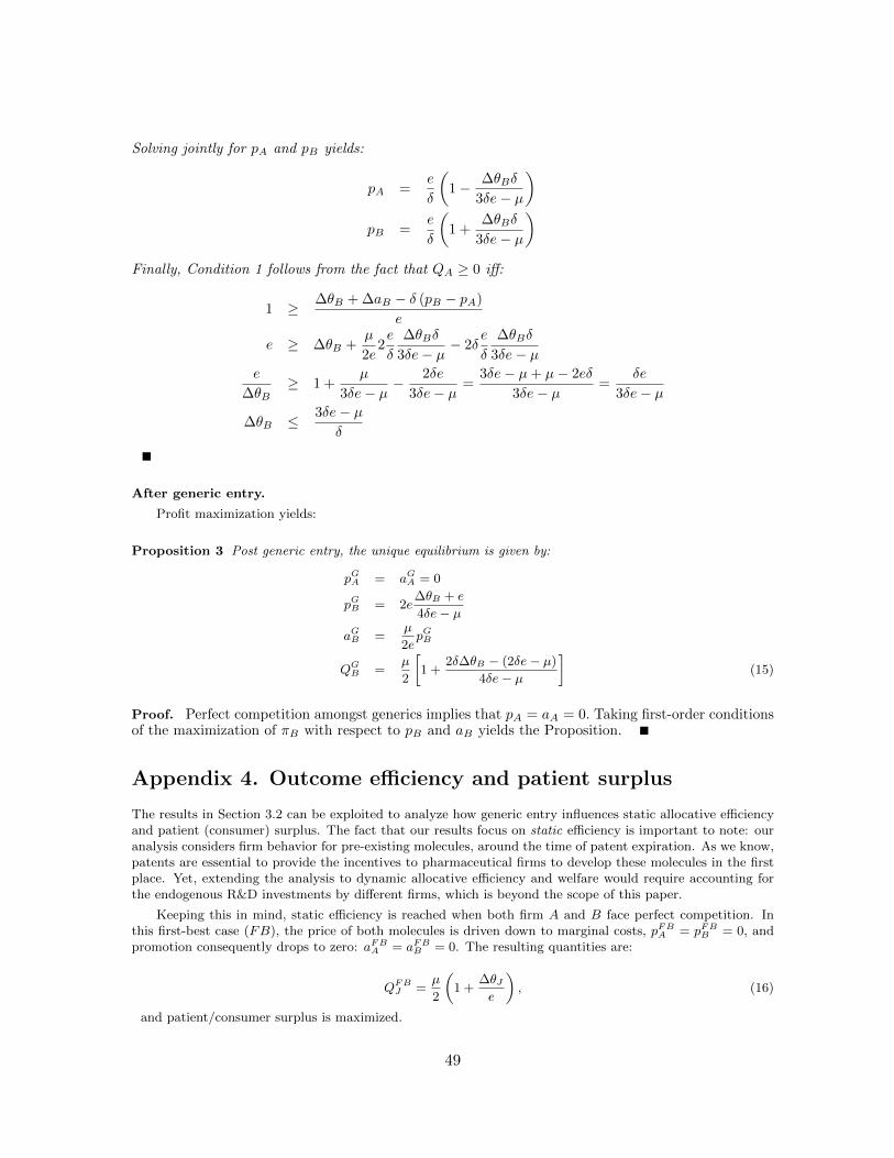
Solving jointly for pA and pB yields:
pA =e
δ
(1− ∆θBδ
3δe− µ
)pB =
e
δ
(1 +
∆θBδ
3δe− µ
)Finally, Condition 1 follows from the fact that QA ≥ 0 iff:
1 ≥ ∆θB + ∆aB − δ (pB − pA)
e
e ≥ ∆θB +µ
2e2e
δ
∆θBδ
3δe− µ− 2δ
e
δ
∆θBδ
3δe− µe
∆θB≥ 1 +
µ
3δe− µ− 2δe
3δe− µ=
3δe− µ+ µ− 2eδ
3δe− µ=
δe
3δe− µ
∆θB ≤ 3δe− µδ
After generic entry.
Profit maximization yields:
Proposition 3 Post generic entry, the unique equilibrium is given by:
pGA = aGA = 0
pGB = 2e∆θB + e
4δe− µ
aGB =µ
2epGB
QGB =µ
2
[1 +
2δ∆θB − (2δe− µ)
4δe− µ
](15)
Proof. Perfect competition amongst generics implies that pA = aA = 0. Taking first-order conditionsof the maximization of πB with respect to pB and aB yields the Proposition.
Appendix 4. Outcome efficiency and patient surplus
The results in Section 3.2 can be exploited to analyze how generic entry influences static allocative efficiencyand patient (consumer) surplus. The fact that our results focus on static efficiency is important to note: ouranalysis considers firm behavior for pre-existing molecules, around the time of patent expiration. As we know,patents are essential to provide the incentives to pharmaceutical firms to develop these molecules in the firstplace. Yet, extending the analysis to dynamic allocative efficiency and welfare would require accounting forthe endogenous R&D investments by different firms, which is beyond the scope of this paper.
Keeping this in mind, static efficiency is reached when both firm A and B face perfect competition. Inthis first-best case (FB), the price of both molecules is driven down to marginal costs, pFBA = pFBB = 0, andpromotion consequently drops to zero: aFBA = aFBB = 0. The resulting quantities are:
QFBJ =µ
2
(1 +
∆θJe
), (16)
and patient/consumer surplus is maximized.
49

Quite trivially, we would reach first best as soon as all molecules have lost exclusivity; it is just a matterof time. In reality, new vintages of old treatments (so-called “me too” drugs) and new treatments appearconstantly. In our quarterly data, for instance, there is at least one molecule still under patent protectionfor all “anatomic therapeutic classes” and periods. That is, reality is best described either by situation Dor situation G that we analyzed above. Our purpose here will be to identify when the movement from D(only patent-protected molecules) to G (some patent-protected molecules) improves market efficiency and/orconsumer surplus. We find that:
Proposition 4 Whether a pharmaceutical firm can (D), or cannot (ND), use detailing, generic entry neverbrings the market equilibrium closer to the first-best allocation (16).
Proof. First, let us concentrate on the case in which firms can use detailing and focus on the quantitiessold by B, since A serves the rest of the market. Consider, first, the case in which qDB > qFBB – i.e.,B sells too much prior to generic entry. By (14) and (16) this only happens if:
δ
3δe− µ>
1
e⇔ 2δe < µ,
which is the exact condition in Proposition 1 for qGB > qDB . Hence, generic entry produces an increasein the quantities sold by B precisely when convergence to the first best requires a drop. By the sametoken, the reverse is true for 2δe > µ.
Second, let us turn to the case in which firms cannot use detailing. As shown in Appendix 1, thequantities before and after generic entry are, respectively:
QDB =µ
2
(1 +
∆θB3e
)QGB =
µ
4
(1 +
∆θBe
)=QFBB
2,
and the condition for QDB and QGB to be less than the whole market (µ) is: ∆θB < 3e. It is straight-forward to check that, for such parameter values, we always have QGB < QDB < QFBB .
The main reason for this result is the same as for Proposition 1: generic entry produces a very asymmetrictype of competition, in which one molecule becomes cheaper but is no longer promoted and the other remainsprotected against direct competition. As we saw, when molecules are distant substitutes and/or market sizeis small (2δe > µ), the genericization of A intensifies competition for B, which loses market share, and cutsdown prices and promotion as a result. This is exactly the intended purpose of generic competition. Theproblem is that this happens precisely when B’s market share is initially lower than in the first best.
Conversely, when the two molecules are close substitutes and/or market size is large (2δe < µ), thegenericization of A actually relaxes the competitive pressure on B. This allows firm B to actually gain marketpower and market share. In this case, firm B also grabs the opportunity to increase its prices and its detailingeffort. This only happens when B’s market share was already initially too high.
Interestingly, prohibiting detailing altogether would not be a panacea. In that case, the market share ofthe more advanced molecule B is always too low (except in the corner solutions in which it grabs 100% of themarket), and the genericization of A further reduces it.
From a policy perspective, being confronted with explosive expenditures on healthcare, authorities haveactively promoted the use of generics, partly in an effort to contain the costs borne (directly or indirectly) bypatients. In addition, competition authorities have, de facto, adopted a consumer surplus standard. We defineconsumer surplus as their utility minus the price they pay for the molecule they actually buy. Importantly,their utility depends on the actual quality of the molecule, θJ , whereas which molecule they actually buy alsodepends on promotion effort, which is rather targeted at the physicians or is spent on the representatives’wages, etc. Thus, we calculate consumer surplus as the integral of the patients’ utilities (1-2) when they
50

actually consume the quantities QDJ before, and QGJ after, generic entry.45 We find that:
Proposition 5 Generic entry necessarily increases consumer welfare when B’s market share (weakly) de-creases after generic entry (i.e., for µ < 2δe). For ∆θB = 0, consumer surplus decreases upon generic entrywhen µ > 2δe
3
(7−√
10)' 2.56 δe, in which case B gains substantial market share, and increases prices and
promotion intensity.
Proof. After tedious algebra (see supplementary material), we find that:
2δe = µ⇒ CWG − CWD =(e− 1)
2
2≥ 0,
where CWD is consumer surplus when both A and B benefit from patent protection, and CWG isconsumer surplus when only B still benefits from patent protection. When µ is smaller, prices mustbe decreasing for all consumers, and their welfare increases.
Imposing ∆θB = 0 for the sake of tractability, one can also identify the value of µ for which thisdifference in consumer surplus is zero. The threshold is: µ = 2δe
3
(7−√
10). For any values of µ below
that threshold, consumer surplus increases upon generic entry.
45 The derivations of consumer surplus are available upon request. We do not present them here becausethey are tedious but rather straightforward.
51

Appendix 5: Supplementary tables
52

53
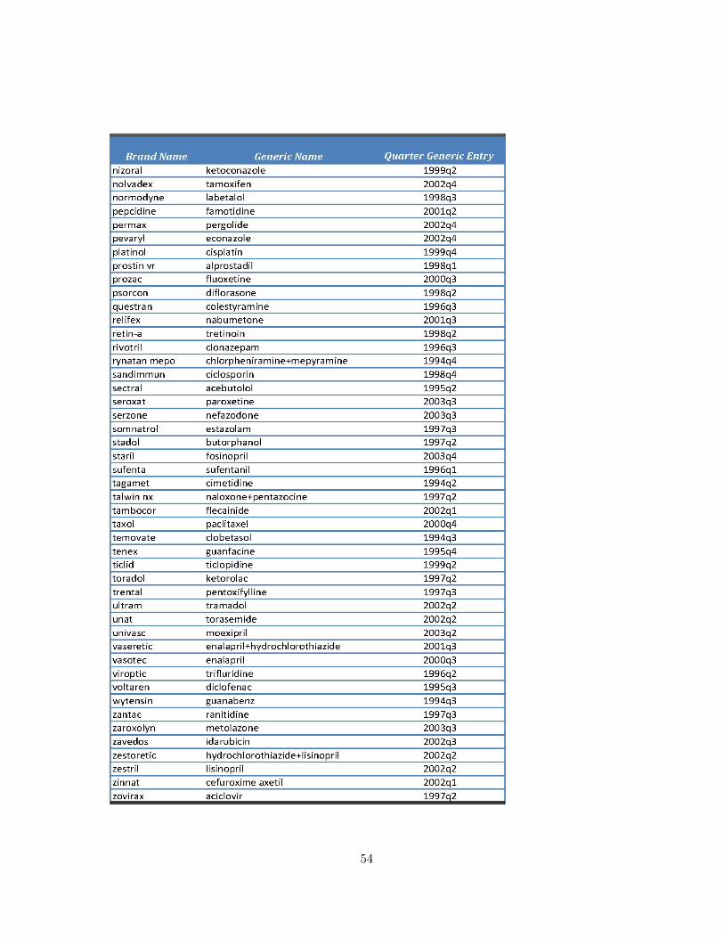
54