the universal relation between exponents in rst …souravc/beam-fpp-trans.pdf · the universal...

The universal relation between exponents infirst-passage percolation

Sourav Chatterjee

(Courant Institute, NYU)

Sourav Chatterjee Exponents in first-passage percolation

First-passage percolation

I Let E (Zd) denote the set of edges in the integer lattice Zd .I Each edge e has a ‘weight’ or ‘passage time’ attached to it,

denoted by te .I Ordinary first-passage percolation assumes that te are i.i.d.

non-negative random variables. Introduced by Hammersley &Welsh (1960).

I The total passage time, or total weight, of a path P is simplythe sum of the weights of the edges in P.

I The first-passage time T (x , y) from a point x to a point y isthe minimum total passage time among all lattice paths fromx to y .

I If the edge-weights are continuous random variables, thenwith probability one there is a unique weight minimizing path(geodesic) between any x and y that we call G (x , y).

I Let D(x , y) denote the maximum deviation of this path fromthe straight line segment joining x and y .


G (x , y) and D(x , y)

x y

D(x, y)

G(x, y)

Figure: The geodesic G (x , y) and the deviation D(x , y).


Exponents

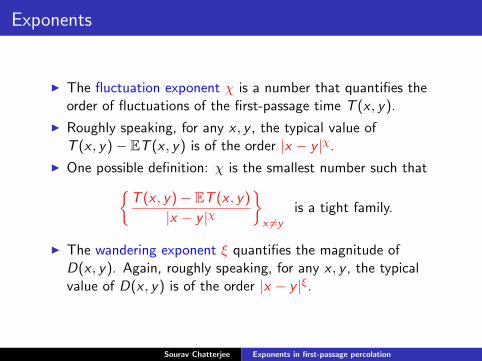
I The fluctuation exponent χ is a number that quantifies theorder of fluctuations of the first-passage time T (x , y).

I Roughly speaking, for any x , y , the typical value ofT (x , y)− ET (x , y) is of the order |x − y |χ.

I One possible definition: χ is the smallest number such that{T (x , y)− ET (x , y)

|x − y |χ

}x 6=y

is a tight family.

I The wandering exponent ξ quantifies the magnitude ofD(x , y). Again, roughly speaking, for any x , y , the typicalvalue of D(x , y) is of the order |x − y |ξ.


The conjectured relation between χ and ξ

I Physicists say that irrespective of the dimension, χ and ξmust satisfy the scaling identity χ = 2ξ − 1.

I Conjectured in numerous physics papers: Huse and Henley(1985), Kardar, Parisi and Zhang (1986), Kardar and Zhang(1987), Krug (1987), Krug and Meakin (1989), Krug andSpohn (1991), Meakin et. al. (1986), Medina et. al. (1989),Wolf and Kertesz (1987), etc. Sometimes called KPZ relation.

I Rigorous literature gives support in one direction only:Newman and Piza (1995) showed that χ′ ≥ 2ξ − 1, where χ′

is a related exponent that may be equal to χ. Earlier, Wehrand Aizenman (1990) proved χ ≥ (1− (d − 1)ξ)/2.

I Wuthrich (1998) proved the opposite inequality forSznitman’s model of Brownian motion in a truncatedPoissonian potential. No results for first-passage percolation.

I In this talk, I will prove the relation χ = 2ξ − 1 assuming thatχ and ξ exist in a certain sense.


Defining χ ‘from above’

I Recall that a family of random variables {Xn} is said to beexponentially tight if there exists α > 0 such that E(eα|Xn|) isuniformly bounded as n varies.

I Kesten (1993) proved that χ ≤ 1/2 in the sense that thefamily {

T (x , y)− ET (x , y)

|x − y |1/2

}x 6=y

is exponentially tight.

I Inspired by Kesten’s result, one may define an exponent χa

‘from above’ to be the infimum of all δ such that the family{T (x , y)− ET (x , y)

|x − y |δ

}x 6=y

is exponentially tight.


Defining χ from below

I It is easy to show under mild assumptions that there is aC > 0 such that for all x 6= y

Var(T (x , y)) ≥ C .

I As before, this inspires the definition of an exponent χb ‘frombelow’ as the supremum of all δ such that for some C > 0, forall x 6= y ,

Var(T (x , y)) ≥ C |x − y |2δ.

I It is easy to show that 0 ≤ χb ≤ χa ≤ 1/2. When χa = χb,we will say that the fluctuation exponent χ exists and equalsthis number.

I The wandering exponent ξ may be defined in a similarmanner, by first defining ξa and ξb, and then saying that ξexists if ξa = ξb.


BKS distributions

I It follows from Kesten’s result that

Var(T (x , y)) ≤ C |x − y |.

I For binary edge weights, this was improved by Benjamini,Kalai and Schramm (2003), using a hypercontractive methodof Talagrand:

Var(T (x , y)) ≤ C|x − y |

log |x − y |.

I We will say that the edge-weight distribution belongs to theBKS class if the above improved bound holds. Thus,two-point distributions belong to the BKS class.

I Benaım and Rossignol (2008) proved that a large class ofdistributions, including the exponential, beta, gamma anduniform distributions, belong to the BKS class.


The main result

Theorem (C., 2011)

Consider first-passage percolation in any dimension ≥ 2. Supposethat the edge-weight distribution is continuous and belongs to theBKS class, and that the exponents χ and ξ exist in the sensedefined before. Then χ = 2ξ − 1.

Remark: Recently, Auffinger and Damron have made an importantimprovement to the proof that removes the BKS assumption. Willsay more about it later.


The functions g and h

I Let h(x) := E(T (0, x)).

I The function h is subadditive. Therefore the limit

g(x) := limn→∞

h(nx)

n

exists for all x ∈ Zd .

I Can be extended to all x ∈ Qd by taking n→∞ through asubsequence.

I Can be extended to all x ∈ Rd by uniform continuity.

I The function g is a norm on Rd .


Approximation of h by g

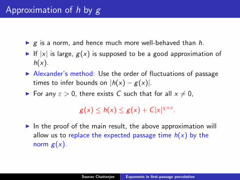
I g is a norm, and hence much more well-behaved than h.

I If |x | is large, g(x) is supposed to be a good approximation ofh(x).

I Alexander’s method: Use the order of fluctuations of passagetimes to infer bounds on |h(x)− g(x)|.

I For any ε > 0, there exists C such that for all x 6= 0,

g(x) ≤ h(x) ≤ g(x) + C |x |χ+ε.

I In the proof of the main result, the above approximation willallow us to replace the expected passage time h(x) by thenorm g(x).


Curvature lemma

I There is a unit vector x0 and a hyperplane H0 perpendicularto x0 such that for some C > 0, for all z ∈ H0,

|g(x0 + z)− g(x0)| ≤ C |z |2.

I There is a unit vector x1 and a hyperplane H1 perpendicularto x1 such that for some C > 0, for all z ∈ H1, |z | ≤ 1,

g(x1 + z) ≥ g(x1) + C |z |2.

I In the direction x0, the unit sphere of the norm g is ‘at mostas curved as an Euclidean sphere’ and in the direction x1, it is‘at least as curved as an Euclidean sphere’.


Idea of the proof of χ ≥ 2ξ − 1

0 nx1mx1

mx1 + z

P

I By the definition of the direction of curvature x1,

Expected passage time of the path P

≥ g(mx1 + z) + g(nx1 − (mx1 + z)) + O(nχ+ε)

≥ E(T (0, nx1)) + C |z |2/n + O(nχ+ε).

I Suppose |z | = nξ. Then |z |2/n = n2ξ−1.I Fluctuations of T (0, nx1) are of order nχ. Thus, if

2ξ − 1 > χ, then P cannot be a geodesic from 0 to nx1.


Proving χ ≤ 2ξ − 1 when χ > 0

0 ax0

2ax0

3ax0

(n− a)x0 nx0

Figure: Solid curve is G (0, nx0). Dashed curves are G (iax0, (i + 1)ax0)

I Recall direction of curvature x0. Let a = nβ, β < 1. Letm = n/a = n1−β.

I Under the condition χ > 2ξ − 1, we will show that there is aβ < 1 such that

T (0, nx0) =m−1∑i=0

T (iax0, (i + 1)ax0) + o(nχ). (?)

This will lead to a contradiction.


Getting a contradiction under (?)

I Let f (n) := VarT (0, nx0). Then by the BKS criterion,f (n) ≤ Cn/ log n.

I Under (?), by the FKG-Harris inequality,

f (n) = VarT (0, nx0) ≥ mVarT (0, ax0) + o(n2χ)

= n1−βf (nβ) + o(n2χ).

I Consequently,

lim infn→∞

f (n)

n1−βf (nβ)≥ 1. (†)

I Choose n0 > 1 and define ni+1 = n1/βi for each i .

I Let v(n) := f (n)/n. Then v(ni ) ≤ C/ log ni ≤ Cβi .I But by (†), lim inf v(ni+1)/v(ni ) ≥ 1, and so for all i large

enough, v(ni+1) ≥ β1/2v(ni ).I In particular, v(ni ) ≥ const.βi/2.I Since β < 1, this gives a contradiction for i large.


Proving (?): Small blocks and big blocks

U0 V0 U1 V1 U2 Vm−1 Um

0 nx0a b

Figure: Cylinder of width nξ around the line joining 0 and nx0

I Let a = nβ and b = nβ′, where β′ < β < 1.

I Consider a cylinder of width nξ around the line joining 0 andnx0.

I Partition the cylinder into alternating big and small cylindersof widths a and b respectively.

I Call the boundary walls of these cylindersU0,V0,U1,V1, . . . ,Vm−1,Um, where m is roughly n1−β.


Approximating by cylinders

U0 V0 U1 V1 U2 Vm−1 Um

0 nx0a b

Figure: Cylinder of width nξ around the line joining 0 and nx0

I Key step: (will skip the proof)∣∣∣∣T (U0,Um)−m−1∑i=0

(T (Ui ,Vi ) + T (Vi ,Ui+1))

∣∣∣∣ ≤ m−1∑i=0

Mi ,

where Mi := maxv ,v ′∈Vi , u,u′∈Ui+1|T (v , u)− T (v ′, u′)|.

I Note that the errors Mi come only from the small blocks.


Proving (?): Estimating the error

v

v′

u

u′

nβ′

nξ

I By curvature estimate in direction x0,

|ET (v , u)− ET (v ′, u′)| ≤ C (nξ)2/nβ′

= Cn2ξ−β′.

I Fluctuations of T (v , u) are of order nβ′χ.

I If 2ξ − 1 < χ, then we can choose β′ so close to 1 that2ξ − β′ < β′χ. That is, fluctuations dominate whileestimating Mi . Consequently, Mi is of order nβ

′χ.I Thus, total error = n1−β+β′χ. Since β′ < β and χ > 0, this

allows us to choose β′, β such that the exponent is < χ. Thisproves (?).

I The above bound has been cleverly used by Auffinger andDamron to get a simpler proof of χ ≤ 2ξ − 1 when χ > 0.


The case χ = 0

I The proof of χ ≤ 2ξ − 1 when χ = 0 is quite different thanthe case χ > 0. I will spare you the details.


A digression: superconcentration and chaos

I It is conjectured that χ = 1/3 and ξ = 2/3 is 2D. It is alsobelieved that χ may be 0 in sufficiently high dimension.

I As stated before, Kesten showed that χ ≤ 1/2. However, it isnot even known whether χ < 1/2 in any dimension.

I The phenomenon that χ < 1/2 is sometimes called ‘sublinearvariance’. I call it ‘superconcentration’. Manifests in manyother models.

I In the related model of last-passage percolation with Gaussianweights, I proved in 2008 that χ = 1

2τ , where τ is an exponentsuch that |P ∩ P ′| is of order nτ , where P is the optimal pathand P ′ is the optimal path in a slightly perturbed environment.

I In other words, χ < 1/2 if and only if τ < 1. The phenomenonτ < 1 is sometimes called ‘chaos’ in such disordered systems.

I Main result of my 2008 paper: superconcentration isequivalent to chaos.


Preprints on arXiv

I S. Chatterjee (2008): Chaos, concentration, and multiplevalleys.

I S. Chatterjee (2011): The universal relation between scalingexponents in first-passage percolation.

I A. Auffinger and M. Damron (2011): A simplified proof of therelation between scaling exponents in first-passage percolation.


the universal relation between exponents in rst …souravc/beam-fpp-trans.pdf · the universal...

Documents