THE UNIVERSITY OF CHICAGO

TWISTED HEISENBERG REPRESENTATIONS AND LOCAL CONDUCTORS

A DISSERTATION SUBMITTED TO

THE FACULTY OF THE DIVISION OF THE PHYSICAL SCIENCES

IN CANDIDACY FOR THE DEGREE OF

DOCTOR OF PHILOSOPHY

DEPARTMENT OF MATHEMATICS

BY

ROMYAR T. SHARIFI

CHICAGO, ILLINOIS

JUNE 1999

To my parents: Hassan and Carol Sharifi.

ACKNOWLEDGEMENTS

I thank my advisor Spencer Bloch for many helpful discussions. I thank Dick Gross

for suggesting this problem to me and for his advice. I thank Rene Schoof for his

suggestions on use of the Hochschild-Serre spectral sequence and Hendrik Lenstra for

advice on the Galois module structure of the multiplicative group of a local field. I

would also like to thank my roommate Andrew Przeworski for listening to me ramble

on about my thesis and trying to help out when he could and my officemate Paul Li

for giving me advice about group theory.

iii

TABLE OF CONTENTS

ACKNOWLEDGEMENTS . . . . . . . . . . . . . . . . . . . . . . . . . . . . iii

INTRODUCTION . . . . . . . . . . . . . . . . . . . . . . . . . . . . . . . . . 1

1 COHOMOLOGICAL RESULTS . . . . . . . . . . . . . . . . . . . . . . . . 71.1 The transgression . . . . . . . . . . . . . . . . . . . . . . . . . . . . . 71.2 Galois embedding problems . . . . . . . . . . . . . . . . . . . . . . . 111.3 Twisted Galois maps . . . . . . . . . . . . . . . . . . . . . . . . . . . 17

2 TWISTED HEISENBERG REPRESENTATIONS . . . . . . . . . . . . . . 212.1 Definitions . . . . . . . . . . . . . . . . . . . . . . . . . . . . . . . . . 212.2 Twisted Kummer representations . . . . . . . . . . . . . . . . . . . . 242.3 Cup product . . . . . . . . . . . . . . . . . . . . . . . . . . . . . . . . 262.4 Three-dimensional Heisenberg representations . . . . . . . . . . . . . 272.5 Three-dimensional twisted Heisenberg representations . . . . . . . . . 292.6 Twisted Heisenberg representations . . . . . . . . . . . . . . . . . . . 31

3 LOCAL FIELDS . . . . . . . . . . . . . . . . . . . . . . . . . . . . . . . . 343.1 The Hochschild-Serre spectral sequence . . . . . . . . . . . . . . . . . 343.2 The spectral sequence for local fields . . . . . . . . . . . . . . . . . . 393.3 Twisted Heisenberg representations . . . . . . . . . . . . . . . . . . . 43

4 RAMIFICATION . . . . . . . . . . . . . . . . . . . . . . . . . . . . . . . . 464.1 Preliminaries . . . . . . . . . . . . . . . . . . . . . . . . . . . . . . . 464.2 The multiplicative group as a module . . . . . . . . . . . . . . . . . . 494.3 Comparison of module structure with unit filtration . . . . . . . . . . 524.4 Conductors in the metabelian case . . . . . . . . . . . . . . . . . . . 534.5 Ramification in a Heisenberg extension . . . . . . . . . . . . . . . . . 58

REFERENCES . . . . . . . . . . . . . . . . . . . . . . . . . . . . . . . . . . . 65

iv

INTRODUCTION

In this thesis, we consider a special class of Galois representations which we call

“twisted Heisenberg representations.” These are modular representations of the ab-

solute Galois group of a field in dimension at least three, providing an interesting

class of examples beyond the often studied two-dimensional representations. We

study these from two perspectives. The first is the point of view of embedding prob-

lems, for which we investigate lifts to twisted Heisenberg representations for fields of

good characteristic. The other is the point of view of number theory, for which we

consider the representations over local fields and study their ramification.

An embedding problem is the attempt to realize a given Galois extension of the

ground field inside a larger extension with predetermined Galois group. The study

of embedding problems dates back to Brauer [1] and even before, with many results,

some quite general, having been proven of the sort which profess existence of a solution

to a given embedding problem [11]. One of the key aspects of our study of lifts to

twisted Heisenberg representations, described in more detail below, is that we can not

only determine conditions for a solution to exist but also give a concrete description

of the fixed fields of the kernels of these representations. We expect this to be one of

many examples of Galois groups for which we will be able to construct solutions to

embedding problems explicitly.

Although obtained entirely independently, our construction generalizes work of

Massy [17], [18], who obtained a constructive solution to the embedding problem for

extra-special p-groups as central extensions of abelian p-groups over fields of charac-

teristic not p containing pth roots of unity. This problem finds it origins in papers

of Dedekind [6], who gave examples of quaternion extensions of Q and Witt, who

solved the embedding problem of the quaternion group of order 8 over the dihedral

group of order 4 [23]. It was then studied in [5], [4], [7] and [19] before Massy gave

his constructive solution. More recently, Swallow [21] has given a solution which is

1

2

in general more explicit than Massy’s, and Brattstrom [2] has studied the case in

which the field is not assumed to contain pth roots of unity (which can be viewed as

a special case of the twisted Heisenberg representations we consider).

Another aspect of the theory of Galois representations is the relationship of Ga-

lois representations with modular forms. This is the subject of several conjectures,

beginning with Serre’s conjecture [16] on two-dimensional Galois representations of

the absolute Galois group of Q. More recently, Gross has made conjectures on the

existence of modular representations associated to modular forms modulo p [9], [10].

In order to obtain results on the existence of modular representations, one can first at-

tempt to determine some information about the representations involved. To do this,

we can describe ramification in the extension given by the fixed of the kernel. We give

an analysis of ramification in the fixed fields of the kernels of certain twisted Heisen-

berg representations of the absolute Galois group of Qp. From the point of view of

local class field theory, this description provides interesting examples of ramification

groups for two and three-step solvable extensions.

Before discussing this thesis in more detail, let us first define the representations

that we will consider. For a field K, we let GK denote its absolute Galois group.

Let E be a field of characteristic not dividing a positive integer m, and let F denote

the cyclotomic extension of E by mth roots of unity. Let Bd denote the subgroup of

upper triangular matrices modulo scalars of PGLd(Z/mZ).

Definition. A twisted Heisenberg representation is a homomorphism ρ : GE → Bd

with the following properties:

(1) The image of GF under ρ is the Heisenberg group Hd of elements of the form

1 ∗ ∗ · · · ∗ ∗1 0 · · · 0 ∗

. . . . . ....

...

1 0 ∗1 ∗

1

.

3

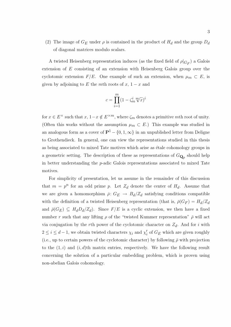
(2) The image of GE under ρ is contained in the product of Hd and the group Dd

of diagonal matrices modulo scalars.

A twisted Heisenberg representation induces (as the fixed field of ρ|GF) a Galois

extension of E consisting of an extension with Heisenberg Galois group over the

cyclotomic extension F/E. One example of such an extension, when µm ⊂ E, is

given by adjoining to E the mth roots of x, 1− x and

c =m∏i=1

(1− ζimm√x)i

for x ∈ E× such that x, 1−x /∈ E×m, where ζm denotes a primitive mth root of unity.

(Often this works without the assumption µm ⊂ E.) This example was studied in

an analogous form as a cover of P1−{0, 1,∞} in an unpublished letter from Deligne

to Grothendieck. In general, one can view the representations studied in this thesis

as being associated to mixed Tate motives which arise as etale cohomology groups in

a geometric setting. The description of these as representations of GQp should help

in better understanding the p-adic Galois representations associated to mixed Tate

motives.

For simplicity of presentation, let us assume in the remainder of this discussion

that m = pn for an odd prime p. Let Zd denote the center of Hd. Assume that

we are given a homomorphism ρ : GE → Bd/Zd satisfying conditions compatible

with the definition of a twisted Heisenberg representation (that is, ρ(GF ) = Hd/Zd

and ρ(GE) ⊆ HdDd/Zd). Since F/E is a cyclic extension, we then have a fixed

number r such that any lifting ρ of the “twisted Kummer representation” ρ will act

via conjugation by the rth power of the cyclotomic character on Zd. And for i with

2 ≤ i ≤ d− 1, we obtain twisted characters χi and χ′i of GE which are given roughly

(i.e., up to certain powers of the cyclotomic character) by following ρ with projection

to the (1, i) and (i, d)th matrix entries, respectively. We have the following result

concerning the solution of a particular embedding problem, which is proven using

non-abelian Galois cohomology.

4

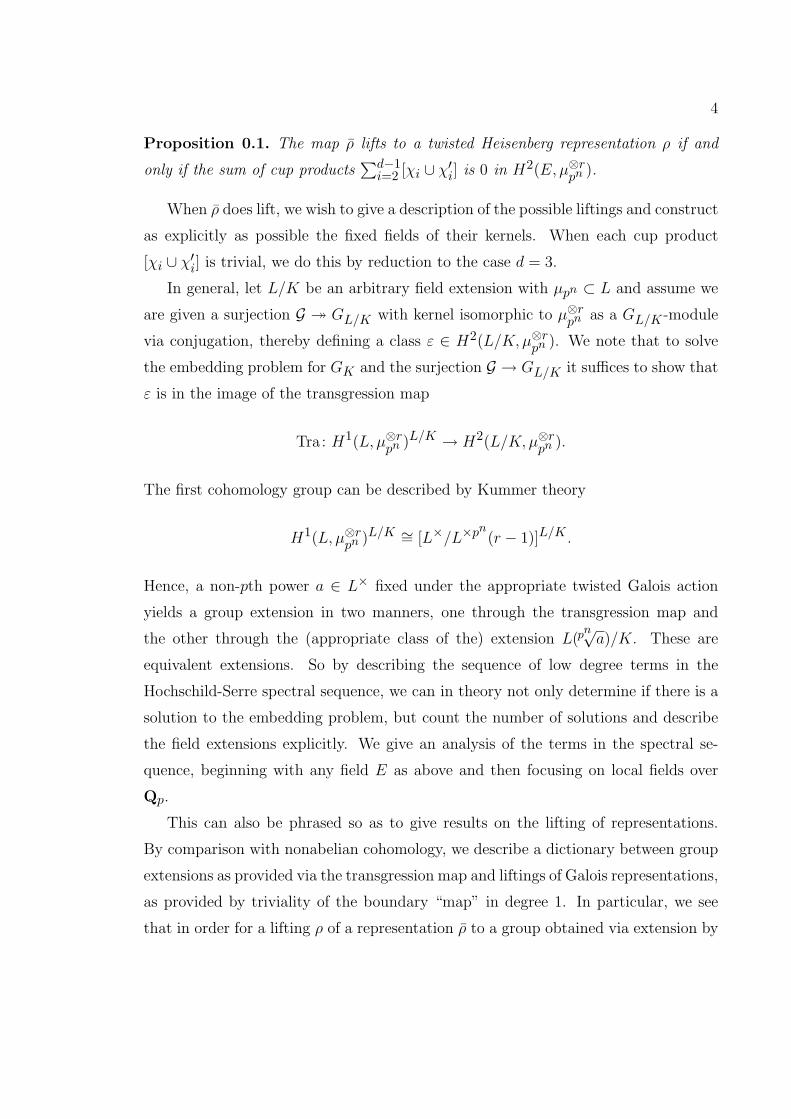
Proposition 0.1. The map ρ lifts to a twisted Heisenberg representation ρ if and

only if the sum of cup products∑d−1i=2 [χi ∪ χ′i] is 0 in H2(E, µ⊗rpn ).

When ρ does lift, we wish to give a description of the possible liftings and construct

as explicitly as possible the fixed fields of their kernels. When each cup product

[χi ∪ χ′i] is trivial, we do this by reduction to the case d = 3.

In general, let L/K be an arbitrary field extension with µpn ⊂ L and assume we

are given a surjection G � GL/K with kernel isomorphic to µ⊗rpn as a GL/K -module

via conjugation, thereby defining a class ε ∈ H2(L/K, µ⊗rpn ). We note that to solve

the embedding problem for GK and the surjection G → GL/K it suffices to show that

ε is in the image of the transgression map

Tra: H1(L, µ⊗rpn )L/K → H2(L/K, µ⊗rpn ).

The first cohomology group can be described by Kummer theory

H1(L, µ⊗rpn )L/K ∼= [L×/L×pn

(r − 1)]L/K .

Hence, a non-pth power a ∈ L× fixed under the appropriate twisted Galois action

yields a group extension in two manners, one through the transgression map and

the other through the (appropriate class of the) extension L(pn√a)/K. These are

equivalent extensions. So by describing the sequence of low degree terms in the

Hochschild-Serre spectral sequence, we can in theory not only determine if there is a

solution to the embedding problem, but count the number of solutions and describe

the field extensions explicitly. We give an analysis of the terms in the spectral se-

quence, beginning with any field E as above and then focusing on local fields over

Qp.

This can also be phrased so as to give results on the lifting of representations.

By comparison with nonabelian cohomology, we describe a dictionary between group

extensions as provided via the transgression map and liftings of Galois representations,

as provided by triviality of the boundary “map” in degree 1. In particular, we see

that in order for a lifting ρ of a representation ρ to a group obtained via extension by

5

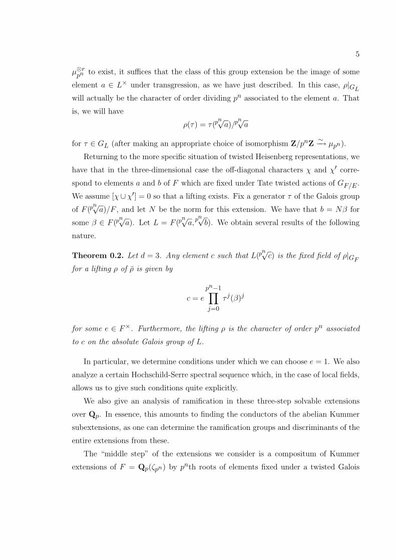
µ⊗rpn to exist, it suffices that the class of this group extension be the image of some

element a ∈ L× under transgression, as we have just described. In this case, ρ|GL

will actually be the character of order dividing pn associated to the element a. That

is, we will have

ρ(τ) = τ(pn√a)/p

n√a

for τ ∈ GL (after making an appropriate choice of isomorphism Z/pnZ∼−→ µpn).

Returning to the more specific situation of twisted Heisenberg representations, we

have that in the three-dimensional case the off-diagonal characters χ and χ′ corre-

spond to elements a and b of F which are fixed under Tate twisted actions of GF/E .

We assume [χ∪ χ′] = 0 so that a lifting exists. Fix a generator τ of the Galois group

of F (pn√a)/F , and let N be the norm for this extension. We have that b = Nβ for

some β ∈ F (pn√a). Let L = F (p

n√a,p

n√b). We obtain several results of the following

nature.

Theorem 0.2. Let d = 3. Any element c such that L(pn√c) is the fixed field of ρ|GF

for a lifting ρ of ρ is given by

c = e

pn−1∏j=0

τ j(β)j

for some e ∈ F×. Furthermore, the lifting ρ is the character of order pn associated

to c on the absolute Galois group of L.

In particular, we determine conditions under which we can choose e = 1. We also

analyze a certain Hochschild-Serre spectral sequence which, in the case of local fields,

allows us to give such conditions quite explicitly.

We also give an analysis of ramification in these three-step solvable extensions

over Qp. In essence, this amounts to finding the conductors of the abelian Kummer

subextensions, as one can determine the ramification groups and discriminants of the

entire extensions from these.

The “middle step” of the extensions we consider is a compositum of Kummer

extensions of F = Qp(ζpn) by pnth roots of elements fixed under a twisted Galois

6

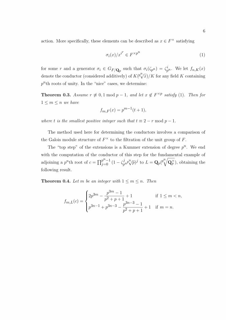
action. More specifically, these elements can be described as x ∈ F× satisfying

σi(x)/xir∈ F×p

n(1)

for some r and a generator σi ∈ GF/Qpsuch that σi(ζpn) = ζipn . We let fn,K(x)

denote the conductor (considered additively) of K(pn√x)/K for any field K containing

pnth roots of unity. In the “nice” cases, we determine:

Theorem 0.3. Assume r 6≡ 0, 1 mod p − 1, and let x 6∈ F×p satisfy (1). Then for

1 ≤ m ≤ n we have

fm,F (x) = pm−1(t+ 1),

where t is the smallest positive integer such that t ≡ 2− r mod p− 1.

The method used here for determining the conductors involves a comparison of

the Galois module structure of F× to the filtration of the unit group of F .

The “top step” of the extensions is a Kummer extension of degree pn. We end

with the computation of the conductor of this step for the fundamental example of

adjoining a pnth root of c =∏pn−1j=0 (1− ζjpnpn√

p)j to L = Qp(pn√

Q×p ), obtaining the

following result.

Theorem 0.4. Let m be an integer with 1 ≤ m ≤ n. Then

fm,L(c) =

2p3m − p3m − 1

p2 + p+ 1+ 1 if 1 ≤ m < n,

p3n−1 + p3n−3 − p3n−3 − 1

p2 + p+ 1+ 1 if m = n.

CHAPTER 1

COHOMOLOGICAL RESULTS

1.1 The transgression

We would like a suitable definition of the transgression map in the Hochschild-Serre

spectral sequence in terms of group extensions. What we obtain is known, but the

author is unaware of a good reference for it. Let G be a profinite group, N an open

normal subgroup of G and A a discrete G-module upon which N acts trivially. From

the Hochschild-Serre spectral sequence we obtain the transgression map

Tra: H1(N,A)G/N → H2(G/N,A).

Koch [12, §3.6] describes this map as follows. For a homomorphism f ∈ H1(N,A)G/N ,

extend f to a continuous map h : G → A satisfying σh(σ−1τσ) = h(τ) and h(τσ) =

h(τ) + h(σ) for all τ ∈ N and σ ∈ G. Then dh induces a well-defined 2-cocycle on

G/N , the class of which is Tra f .

In terms of group extensions, we can express this as follows. For f ∈ H1(N,A)G/N ,

define g : N → AoG by g(τ) = (f(τ), τ). Then g(N) is normal in AoG, so define

E = (A o G)/g(N). This yields the following commutative diagram, in which the

upper exact sequence induces the lower exact sequence (∗)

0 // A // AoG //

��

G //

����

1

0 // A // E // G/N // 1 (∗).

The maps in the lower sequence are well-defined and (∗) is exact. To see this, note

that for a ∈ A and τ ∈ N we have

(a, τ)(f(τ), τ)−1 = (a− f(τ), 1)

7

8

so

π(a, τ) = π(a− f(τ), 1). (1.1)

Alternatively, we can describe E as the pushout in the following commutative diagram

1 // N //

−f��

G //

��

G/N // 1

0 // A // E // G/N // 1 (∗).

(1.2)

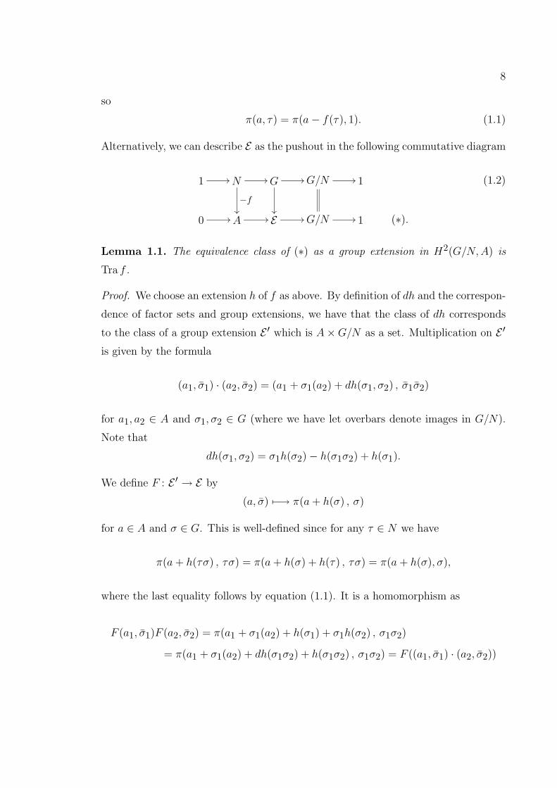
Lemma 1.1. The equivalence class of (∗) as a group extension in H2(G/N,A) is

Tra f .

Proof. We choose an extension h of f as above. By definition of dh and the correspon-

dence of factor sets and group extensions, we have that the class of dh corresponds

to the class of a group extension E ′ which is A×G/N as a set. Multiplication on E ′

is given by the formula

(a1, σ1) · (a2, σ2) = (a1 + σ1(a2) + dh(σ1, σ2) , σ1σ2)

for a1, a2 ∈ A and σ1, σ2 ∈ G (where we have let overbars denote images in G/N).

Note that

dh(σ1, σ2) = σ1h(σ2)− h(σ1σ2) + h(σ1).

We define F : E ′ → E by

(a, σ) 7−→ π(a+ h(σ) , σ)

for a ∈ A and σ ∈ G. This is well-defined since for any τ ∈ N we have

π(a+ h(τσ) , τσ) = π(a+ h(σ) + h(τ) , τσ) = π(a+ h(σ), σ),

where the last equality follows by equation (1.1). It is a homomorphism as

F (a1, σ1)F (a2, σ2) = π(a1 + σ1(a2) + h(σ1) + σ1h(σ2) , σ1σ2)

= π(a1 + σ1(a2) + dh(σ1σ2) + h(σ1σ2) , σ1σ2) = F ((a1, σ1) · (a2, σ2))

9

It is easily checked that F is an isomorphism and induces the identity map on A and

G/N .

We make the following notational conventions for a given field K. We let GK de-

note the Galois group of the separable closure of K over itself. For a Galois extension

L/K, we let GL/K denote its Galois group. For a module A of GK , we denote the

Galois cohomology groups of GK with coefficients in A by H∗(K,A) and we let AK

denote the group of invariants of A under GK . Similarly, if A is a GL/K -module,

we denote the corresponding cohomology groups by H∗(L/K,A) and invariants by

AL/K .

Fix a positive integer m. If K is a field of characteristic prime to m, we let µm

denote the group of mth roots of unity in a separable closure of K. The cyclotomic

character ω : GK → (Z/mZ)∗ is defined by σ(ζm) = ζω(σ)m for a primitive mth root

of unity ζm and σ ∈ GL/K . Let F = K(ζm) denote the fixed field of ω.

In the case that L is a Galois extension of F , a homomorphism ψ : GK → (Z/mZ)∗

with kernel containing GL provides Z/mZ with a GL/K -module structure given by

σ(a) = ψ(σ|L) ·a for a ∈ Z/mZ. We denote this module by Z/mZ(ψ) and the various

cohomology groups with coefficients in Z/mZ(ψ) by H∗(L/K,ψ) (and H∗(K,ψ)).

Tensoring with a GL/K -module A yields a twisted module which we denote A(ψ).

We often use A(r) to denote A(ωr).

Fix a finite Galois extension L/K and a character ψ as above. We have

H1(L, ψ) ∼= (L×/L×m)(ψω−1)

as GL/K -modules via Kummer theory. Explicitly, this is induced by a homomorphism

ϕ : L× → H1(L, µm) (1.3)

defined by ϕ(x) = fx with fx(τ) = τ(m√x)/m√x for τ ∈ GL.

At this point, there arises a certain non-canonical aspect to our approach because,

for any character ψ, we would like to describe a homomorphism ϕ : L× � H1(L, ψ)

as in (1.3). To avoid having to make choices later, we fix for each field K once and

10

for all an isomorphism of groups Z/mZ→ µm compatible with containment of fields.

That is, we identify 1 with ζm for a fixed primitive root of unity ζm in K. We

denote the inverse of this map by Ind = Indζm . Furthermore, for varying m these

isomorphisms should be compatible in the sense that if l divides m then ζm/lm = ζl. In

the case we have just described, this provides fixed (compatible) group isomorphisms

H1(L, µm)∼−→ H1(L, ψ) for each ψ, allowing us to define ϕ from the map described

in 1.3. Again, we set fx = ϕ(x).

For x ∈ L×, let x denote its homomorphic image in L×/L×m. We let

(L/K)ψ = {x ∈ L× | σ(x)ψ(σ) = xω(σ) for all σ ∈ GK}. (1.4)

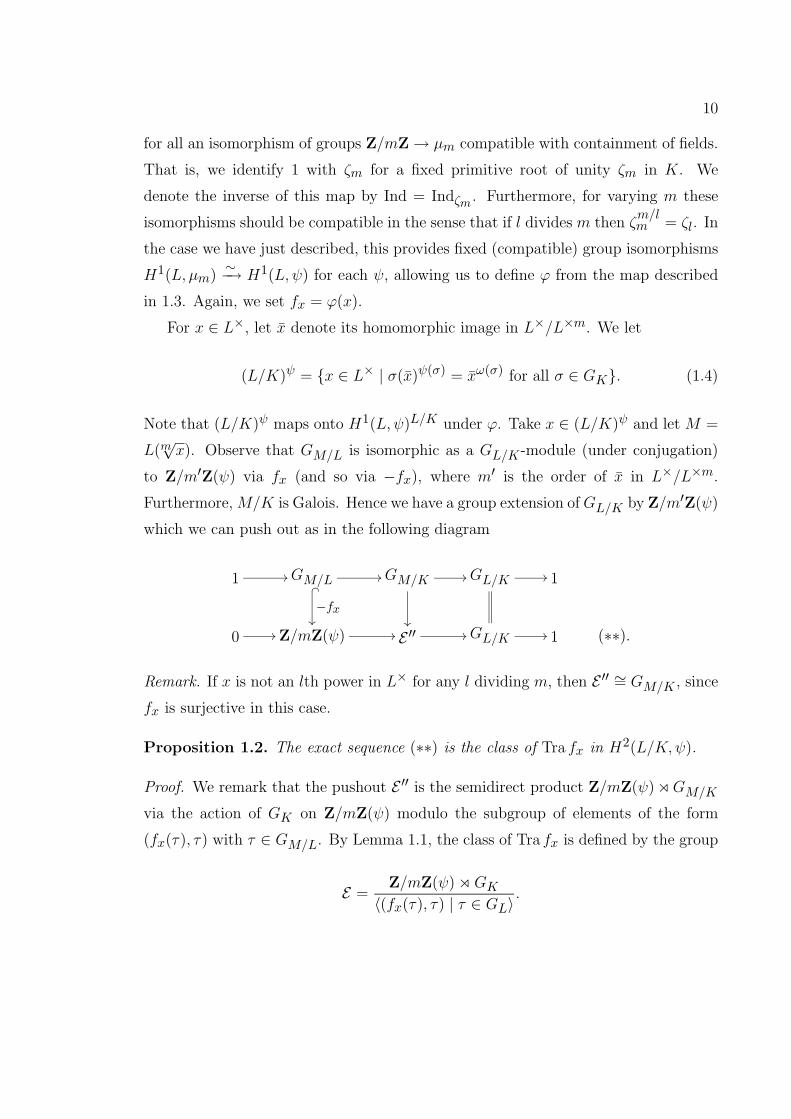
Note that (L/K)ψ maps onto H1(L, ψ)L/K under ϕ. Take x ∈ (L/K)ψ and let M =

L(m√x). Observe that GM/L is isomorphic as a GL/K -module (under conjugation)

to Z/m′Z(ψ) via fx (and so via −fx), where m′ is the order of x in L×/L×m.

Furthermore, M/K is Galois. Hence we have a group extension ofGL/K by Z/m′Z(ψ)

which we can push out as in the following diagram

1 // GM/L //� _

−fx��

GM/K //

��

GL/K // 1

0 // Z/mZ(ψ) // E ′′ // GL/K // 1 (∗∗).

Remark. If x is not an lth power in L× for any l dividing m, then E ′′ ∼= GM/K , since

fx is surjective in this case.

Proposition 1.2. The exact sequence (∗∗) is the class of Tra fx in H2(L/K,ψ).

Proof. We remark that the pushout E ′′ is the semidirect product Z/mZ(ψ) oGM/K

via the action of GK on Z/mZ(ψ) modulo the subgroup of elements of the form

(fx(τ), τ) with τ ∈ GM/L. By Lemma 1.1, the class of Tra fx is defined by the group

E =Z/mZ(ψ) oGK〈(fx(τ), τ) | τ ∈ GL〉

.

11

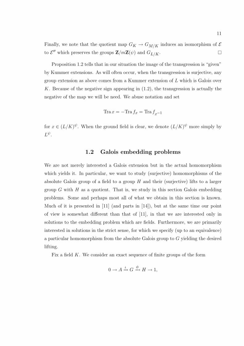
Finally, we note that the quotient map GK → GM/K induces an isomorphism of Eto E ′′ which preserves the groups Z/mZ(ψ) and GL/K .

Proposition 1.2 tells that in our situation the image of the transgression is “given”

by Kummer extensions. As will often occur, when the transgression is surjective, any

group extension as above comes from a Kummer extension of L which is Galois over

K. Because of the negative sign appearing in (1.2), the transgression is actually the

negative of the map we will be need. We abuse notation and set

Trax = −Tra fx = Tra fx−1

for x ∈ (L/K)ψ. When the ground field is clear, we denote (L/K)ψ more simply by

Lψ.

1.2 Galois embedding problems

We are not merely interested a Galois extension but in the actual homomorphism

which yields it. In particular, we want to study (surjective) homomorphisms of the

absolute Galois group of a field to a group H and their (surjective) lifts to a larger

group G with H as a quotient. That is, we study in this section Galois embedding

problems. Some and perhaps most all of what we obtain in this section is known.

Much of it is presented in [11] (and parts in [14]), but at the same time our point

of view is somewhat different than that of [11], in that we are interested only in

solutions to the embedding problem which are fields. Furthermore, we are primarily

interested in solutions in the strict sense, for which we specify (up to an equivalence)

a particular homomorphism from the absolute Galois group to G yielding the desired

lifting.

Fix a field K. We consider an exact sequence of finite groups of the form

0→ Aι−→ G

φ−→ H → 1,

12

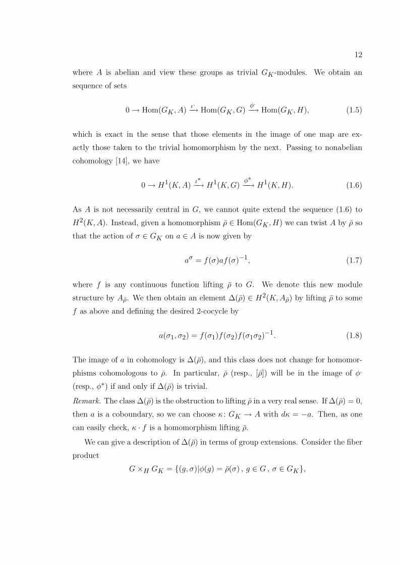
where A is abelian and view these groups as trivial GK -modules. We obtain an

sequence of sets

0→ Hom(GK , A)ι.−→ Hom(GK , G)

φ.

−→ Hom(GK , H), (1.5)

which is exact in the sense that those elements in the image of one map are ex-

actly those taken to the trivial homomorphism by the next. Passing to nonabelian

cohomology [14], we have

0→ H1(K,A)ι∗−→ H1(K,G)

φ∗−−→ H1(K,H). (1.6)

As A is not necessarily central in G, we cannot quite extend the sequence (1.6) to

H2(K,A). Instead, given a homomorphism ρ ∈ Hom(GK , H) we can twist A by ρ so

that the action of σ ∈ GK on a ∈ A is now given by

aσ = f(σ)af(σ)−1, (1.7)

where f is any continuous function lifting ρ to G. We denote this new module

structure by Aρ. We then obtain an element ∆(ρ) ∈ H2(K,Aρ) by lifting ρ to some

f as above and defining the desired 2-cocycle by

a(σ1, σ2) = f(σ1)f(σ2)f(σ1σ2)−1. (1.8)

The image of a in cohomology is ∆(ρ), and this class does not change for homomor-

phisms cohomologous to ρ. In particular, ρ (resp., [ρ]) will be in the image of φ.

(resp., φ∗) if and only if ∆(ρ) is trivial.

Remark. The class ∆(ρ) is the obstruction to lifting ρ in a very real sense. If ∆(ρ) = 0,

then a is a coboundary, so we can choose κ : GK → A with dκ = −a. Then, as one

can easily check, κ · f is a homomorphism lifting ρ.

We can give a description of ∆(ρ) in terms of group extensions. Consider the fiber

product

G×H GK = {(g, σ)|φ(g) = ρ(σ) , g ∈ G , σ ∈ GK},

13

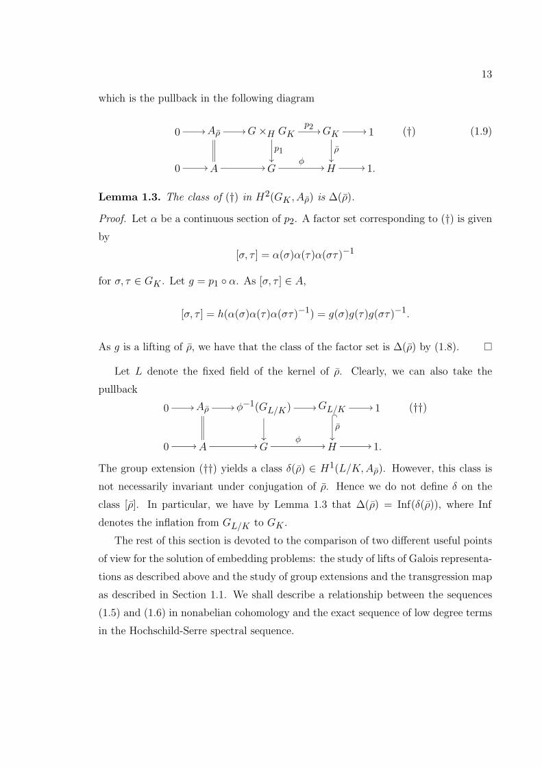
which is the pullback in the following diagram

0 // Aρ // G×H GKp2 //

p1��

GK //

ρ��

1 (†)

0 // A // Gφ

// H // 1.

(1.9)

Lemma 1.3. The class of (†) in H2(GK , Aρ) is ∆(ρ).

Proof. Let α be a continuous section of p2. A factor set corresponding to (†) is given

by

[σ, τ ] = α(σ)α(τ)α(στ)−1

for σ, τ ∈ GK . Let g = p1 ◦ α. As [σ, τ ] ∈ A,

[σ, τ ] = h(α(σ)α(τ)α(στ)−1) = g(σ)g(τ)g(στ)−1.

As g is a lifting of ρ, we have that the class of the factor set is ∆(ρ) by (1.8).

Let L denote the fixed field of the kernel of ρ. Clearly, we can also take the

pullback

0 // Aρ // φ−1(GL/K) //

��

GL/K //� _

ρ��

1 (††)

0 // A // Gφ

// H // 1.

The group extension (††) yields a class δ(ρ) ∈ H1(L/K,Aρ). However, this class is

not necessarily invariant under conjugation of ρ. Hence we do not define δ on the

class [ρ]. In particular, we have by Lemma 1.3 that ∆(ρ) = Inf(δ(ρ)), where Inf

denotes the inflation from GL/K to GK .

The rest of this section is devoted to the comparison of two different useful points

of view for the solution of embedding problems: the study of lifts of Galois representa-

tions as described above and the study of group extensions and the transgression map

as described in Section 1.1. We shall describe a relationship between the sequences

(1.5) and (1.6) in nonabelian cohomology and the exact sequence of low degree terms

in the Hochschild-Serre spectral sequence.

14

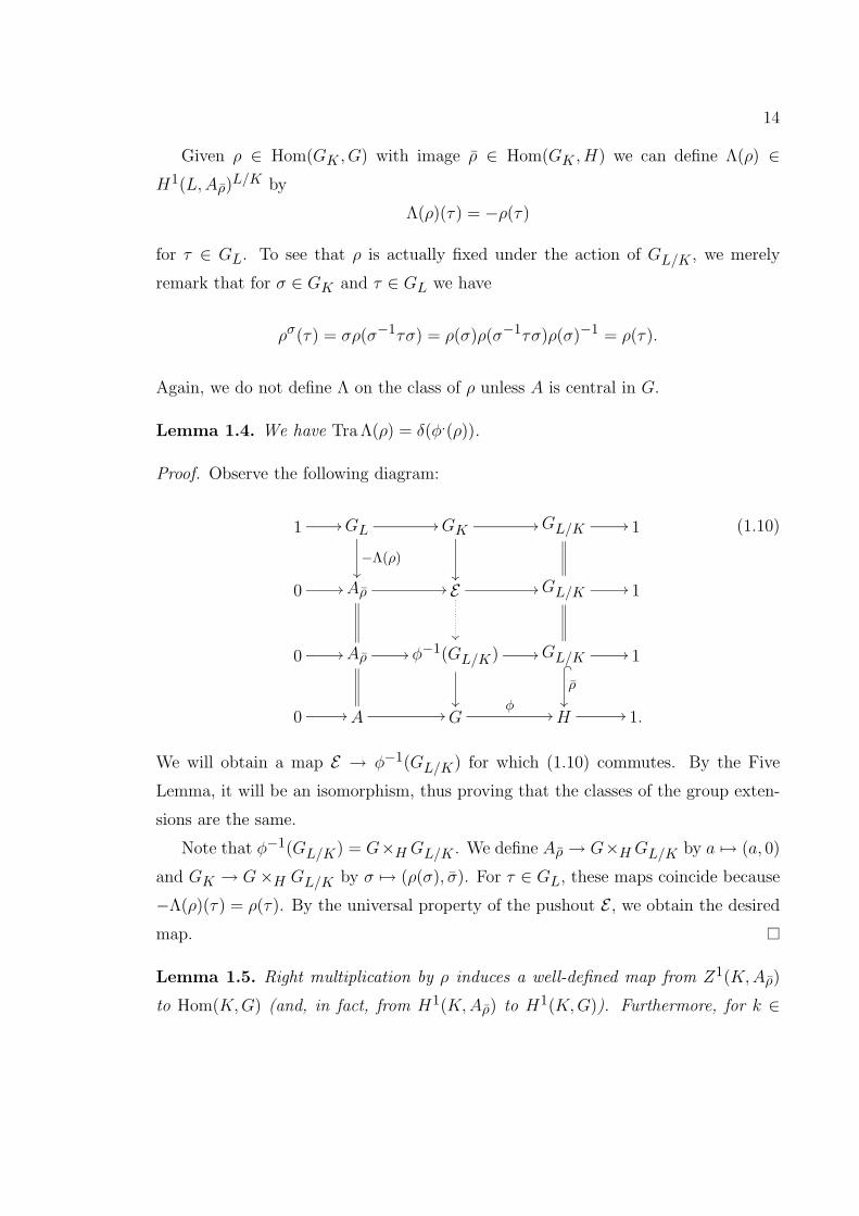
Given ρ ∈ Hom(GK , G) with image ρ ∈ Hom(GK , H) we can define Λ(ρ) ∈H1(L,Aρ)

L/K by

Λ(ρ)(τ) = −ρ(τ)

for τ ∈ GL. To see that ρ is actually fixed under the action of GL/K , we merely

remark that for σ ∈ GK and τ ∈ GL we have

ρσ(τ) = σρ(σ−1τσ) = ρ(σ)ρ(σ−1τσ)ρ(σ)−1 = ρ(τ).

Again, we do not define Λ on the class of ρ unless A is central in G.

Lemma 1.4. We have Tra Λ(ρ) = δ(φ.(ρ)).

Proof. Observe the following diagram:

1 // GL //

−Λ(ρ)��

GK //

��

GL/K // 1

0 // Aρ // E //

��

GL/K // 1

0 // Aρ // φ−1(GL/K) //

��

GL/K //� _

ρ��

1

0 // A // Gφ

// H // 1.

(1.10)

We will obtain a map E → φ−1(GL/K) for which (1.10) commutes. By the Five

Lemma, it will be an isomorphism, thus proving that the classes of the group exten-

sions are the same.

Note that φ−1(GL/K) = G×HGL/K . We define Aρ → G×HGL/K by a 7→ (a, 0)

and GK → G×H GL/K by σ 7→ (ρ(σ), σ). For τ ∈ GL, these maps coincide because

−Λ(ρ)(τ) = ρ(τ). By the universal property of the pushout E , we obtain the desired

map.

Lemma 1.5. Right multiplication by ρ induces a well-defined map from Z1(K,Aρ)

to Hom(K,G) (and, in fact, from H1(K,Aρ) to H1(K,G)). Furthermore, for k ∈

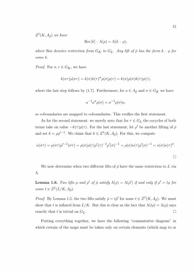
15

Z1(K,Aρ) we have

Res [k] · Λ(ρ) = Λ(k · ρ),

where Res denotes restriction from GK to GL. Any lift of ρ has the form k · ρ for

some k.

Proof. For σ, τ ∈ GK , we have

k(στ)ρ(στ) = k(σ)k(τ)σρ(σ)ρ(τ) = k(σ)ρ(σ)k(τ)ρ(τ),

where the last step follows by (1.7). Furthermore, for a ∈ Aρ and σ ∈ GK we have

a−1aσρ(σ) = a−1ρ(σ)a,

so coboundaries are mapped to coboundaries. This verifies the first statement.

As for the second statement, we merely note that for τ ∈ GL the cocycles of both

terms take on value −k(τ)ρ(τ). For the last statement, let ρ′ be another lifting of ρ

and set k = ρρ′−1. We claim that k ∈ Z1(K,Aρ). For this, we compute

κ(στ) = ρ(στ)ρ′−1(στ) = ρ(σ)ρ(τ)ρ′(τ)−1ρ′(σ)−1 = ρ(σ)κ(τ)ρ′(σ)−1 = κ(σ)κ(τ)σ.

We now determine when two different lifts of ρ have the same restriction to L via

Λ.

Lemma 1.6. Two lifts ρ and ρ′ of ρ satisfy Λ(ρ) = Λ(ρ′) if and only if ρ′ = tρ for

some t ∈ Z1(L/K,Aρ).

Proof. By Lemma 1.5, the two lifts satisfy ρ = tρ′ for some t ∈ Z1(K,Aρ). We must

show that t is inflated from L/K. But this is clear as the fact that Λ(tρ) = Λ(ρ) says

exactly that t is trivial on GL.

Putting everything together, we have the following “commutative diagram” in

which certain of the maps must be taken only on certain elements (which map to or

16

come from ρ or a lift ρ of it) and in which exactness holds only in the appropriate sense

and where appropriate. We include it merely to summarize what we have defined and

proven above:

Z1(L/K,Aρ)� � //

����

Z1(K,Aρ)� � ι. //

����

Hom(GK , G)φ.

//

��

Hom(GK , H) ∆ //

�

H2(K,Aρ)

H1(L/K,Aρ)� � Inf // H1(K,Aρ)

Res // H1(L,Aρ)L/K Tra // H2(L/K,Aρ)

Inf // H2(K,Aρ).

(1.11)

In particular, we obtain the following proposition which relates liftings of Galois

representations to group extensions.

Proposition 1.7. Let ρ : GK → H, and let L denote the fixed field of its kernel. Then

ρ lifts to some ρ : GK → G if and only if δ(ρ) is in the image of the transgression

map. If δ(ρ) = Tra ξ then ρ may be chosen so that Λ(ρ) = ξ. The choice of ρ is

unique up to left multiplication by a cocycle in Z1(L/K,Aρ). Furthermore, ρ will be

surjective if and only if both ρ and ξ are surjective.

Proof. If ρ lifts to ρ then δ(ρ) = Tra (Λ(ρ)) by Lemma 1.4. If, conversely, δ(ρ) = Tra ξ

with ξ ∈ H1(L,Aρ)L/K then

∆(ρ) = Inf ◦ Tra ξ = 0,

so ρ lifts. In this case, let ρ′ be a lifting of ρ. Since

Tra Λ(ρ′) = δ(ρ) = Tra ξ,

we have that Res [k] · Λ(ρ′) = ξ for some k ∈ Z1(K,Aρ). Set ρ = kρ′. From Lemma

1.5 we conclude that Λ(ρ) = ξ. The statement of uniqueness is just Lemma 1.6, and

the last statement is clear.

Remark. In the case A is central in G, the module Aρ is just A with trivial action, and

all the maps we defined above pass to cohomology classes. Hence we obtain another

17

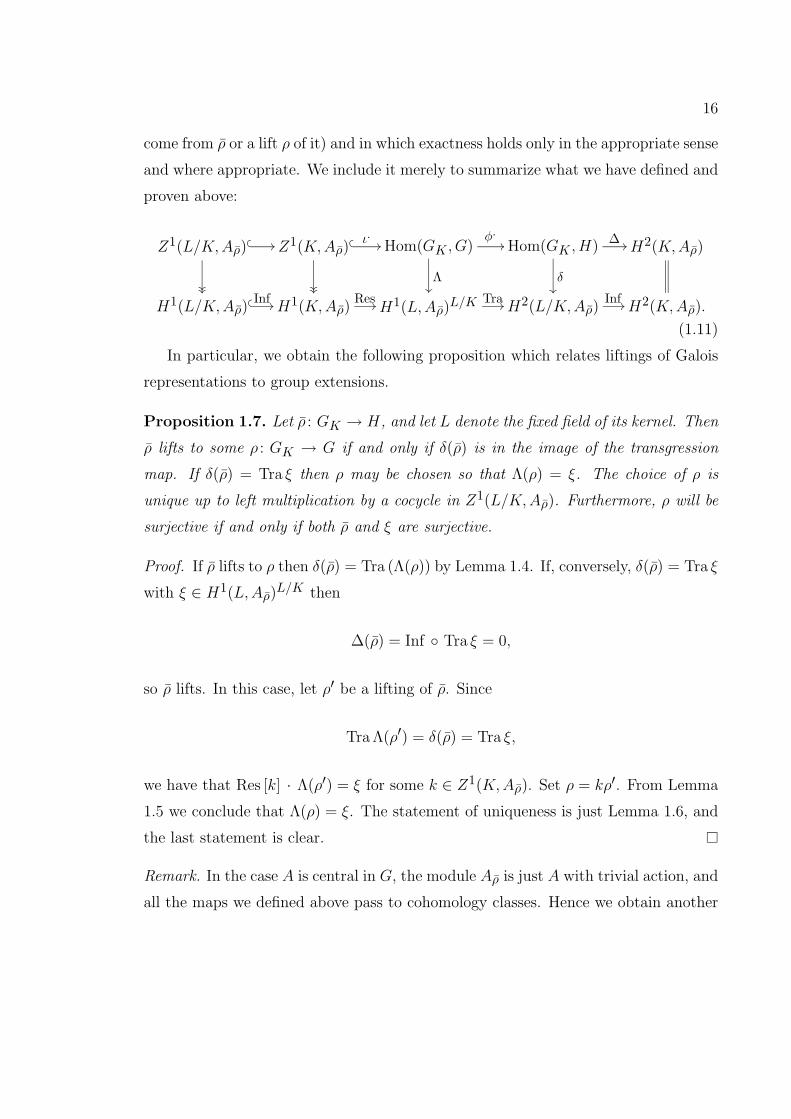
“commutative diagram,” similar to (1.11), in which all the maps in the top row are

defined on all elements:

0 // H1(K,A)ι∗ // H1(K,G)

φ∗//

��

H1(K,H)∆ //

�

H2(K,A)

0 // H1(L/K,A)Inf // H1(K,A)

Res// H1(L,A)L/KTra// H2(L/K,A)

Inf // H2(K,A).

1.3 Twisted Galois maps

Let m be a fixed positive integer and E a field of characteristic not dividing m.

Set F = E(ζm). Let N be a finite nilpotent group with a minimal generating set

S consisting of elements of exponent dividing m. We fix, if possible, an action of

(Z/mZ)∗ on N such that all of the cyclic subgroups generated by the elements of S

are closed under this action. With this action, we define G = N o (Z/mZ)∗. We

define a twisted Galois map with group N to be a homomorphism ρ : GE → G (for

some such G) satisfying ρ(GF ) = N and such that the projection of ρ to (Z/mZ)∗ is

the cyclotomic character ω. The image of a twisted Galois map with group N and a

fixed action is therefore dependent only on the field E, and we denote it by GE . Note

that GE ∼= N oGF/E .

Let c ∈ S and assume c is central in N , generating a cyclic subgroup C of order

l dividing m. Note that G/C = N /C o (Z/mZ)∗. Assume we are given a twisted

Galois representation ρ with group N /C. This defines an action of GE on C given

by a twist of the cyclotomic character. That is, C is isomorphic to Z/lZ(ψ) for some

twist ψ : GF/E → (Z/lZ)∗ and we fix an isomorphism identifying C with this module,

taking c to 1. To see when ρ lifts to a twisted Galois representation with group N ,

we apply the discussions of Sections 1.1 and 1.2.

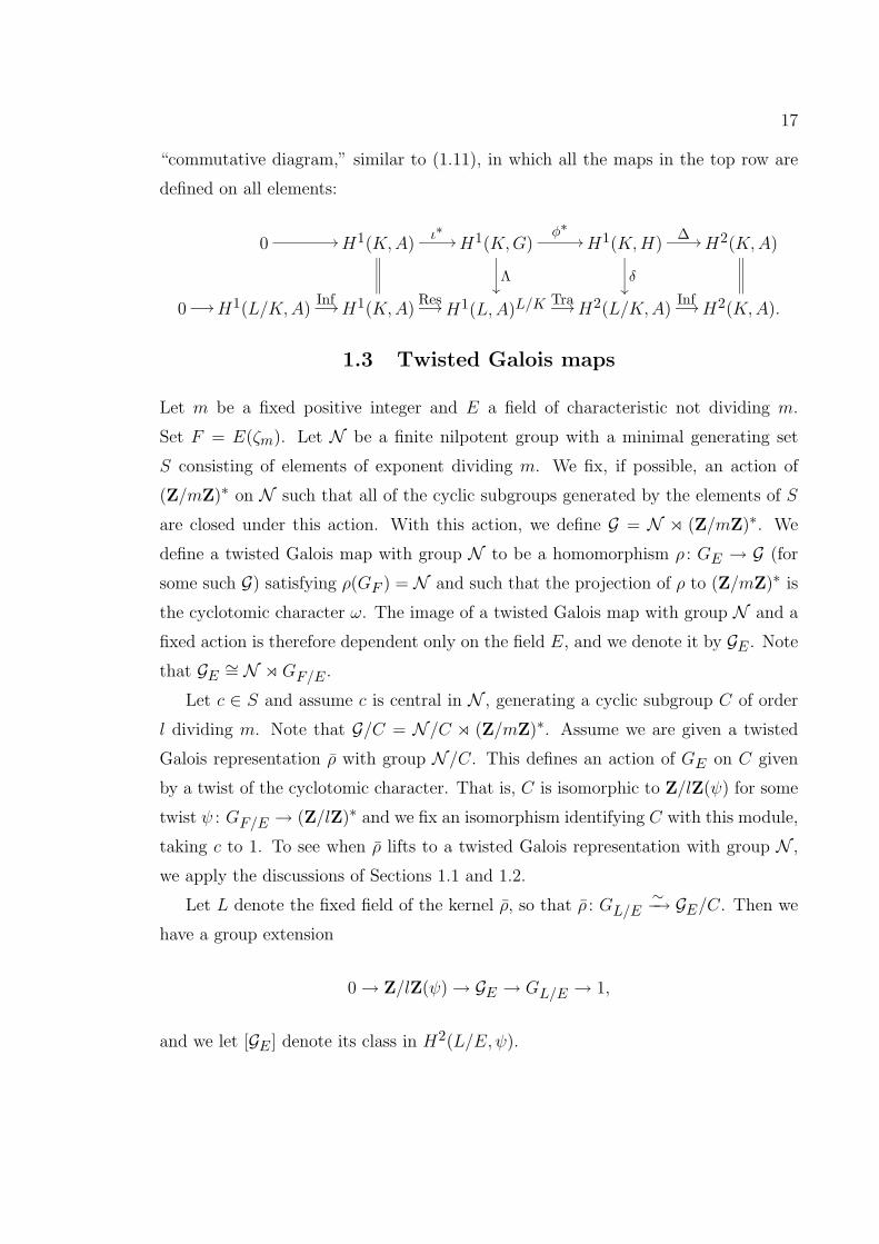
Let L denote the fixed field of the kernel ρ, so that ρ : GL/E∼−→ GE/C. Then we

have a group extension

0→ Z/lZ(ψ)→ GE → GL/E → 1,

and we let [GE ] denote its class in H2(L/E, ψ).

18

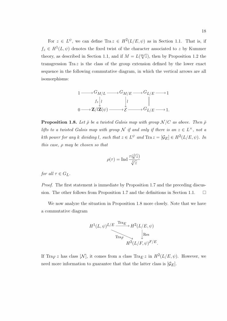
For z ∈ Lψ, we can define Tra z ∈ H2(L/E, ψ) as in Section 1.1. That is, if

fz ∈ H1(L, ψ) denotes the fixed twist of the character associated to z by Kummer

theory, as described in Section 1.1, and if M = L(m√z), then by Proposition 1.2 the

transgression Tra z is the class of the group extension defined by the lower exact

sequence in the following commutative diagram, in which the vertical arrows are all

isomorphisms:

1 // GM/L //

ofz��

GM/E //

o��

GL/E // 1

0 // Z/lZ(ψ) // E // GL/E // 1.

Proposition 1.8. Let ρ be a twisted Galois map with group N /C as above. Then ρ

lifts to a twisted Galois map with group N if and only if there is an z ∈ L×, not a

kth power for any k dividing l, such that z ∈ Lψ and Tra z = [GE ] ∈ H2(L/E, ψ). In

this case, ρ may be chosen so that

ρ(τ) = Indτ( l√z)

l√z

for all τ ∈ GL.

Proof. The first statement is immediate by Proposition 1.7 and the preceding discus-

sion. The other follows from Proposition 1.7 and the definitions in Section 1.1.

We now analyze the situation in Proposition 1.8 more closely. Note that we have

a commutative diagram

H1(L, ψ)L/ETraE //

TraF ((QQQQQQQQQQQQQH2(L/E, ψ)

Res��

H2(L/F, ψ)F/E .

If TraF z has class [N ], it comes from a class TraE z in H2(L/E, ψ). However, we

need more information to guarantee that that the latter class is [GE ].

19

Note that as GF/E sits (non-canonically) as a subgroup of GE . Under ρ, it can be

identified with a subgroup of GL/E with a fixed field E′. We then have a restriction

homomorphism

ResF : H2(L/E, ψ)→ H2(L/E′, ψ) ∼= H2(F/E, ψ).

Though as a map to H2(F/E, ψ) this may not be canonical, it always has the same

kernel. Note that [GE ] will be taken to zero under this homomorphism.

Proposition 1.9. Let ρ be a twisted Galois map with group N /C as above. Then

ρ lifts to a twisted Galois map with group N if and only if there is a z ∈ L×, not

a kth power for any k dividing l, satisfying z ∈ Lψ and such that TraF z = [N ] ∈H2(L/F, ψ) and ResF ◦TraE z = 0.

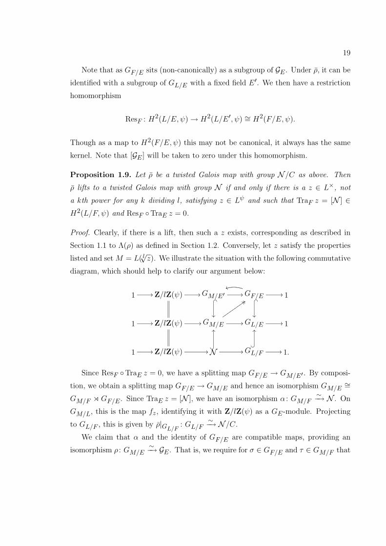
Proof. Clearly, if there is a lift, then such a z exists, corresponding as described in

Section 1.1 to Λ(ρ) as defined in Section 1.2. Conversely, let z satisfy the properties

listed and set M = L( l√z). We illustrate the situation with the following commutative

diagram, which should help to clarify our argument below:

1 // Z/lZ(ψ) // GM/E′ //� _

��

GF/E //

tt

� _

��

1

1 // Z/lZ(ψ) // GM/E //

:: ::vvvvvvvvvGL/E // 1

1 // Z/lZ(ψ) // N //?�

OO

GL/F //?�

OO

1.

Since ResF ◦TraE z = 0, we have a splitting map GF/E → GM/E′ . By composi-

tion, we obtain a splitting map GF/E → GM/E and hence an isomorphism GM/E∼=

GM/F o GF/E . Since TraE z = [N ], we have an isomorphism α : GM/F∼−→ N . On

GM/L, this is the map fz, identifying it with Z/lZ(ψ) as a GE-module. Projecting

to GL/F , this is given by ρ|GL/F: GL/F

∼−→ N /C.

We claim that α and the identity of GF/E are compatible maps, providing an

isomorphism ρ : GM/E∼−→ GE . That is, we require for σ ∈ GF/E and τ ∈ GM/F that

20

α(στσ−1) = σα(τ)σ−1. This follows from the identification of GM/L with Z/lZ(ψ)

and the fact that ρ is a homomorphism on GL/E . At the same time, this argument

insures that the isomorphism ρ provides an equality of classes in H2(L/E, ψ).

Given the group PGLd(Z/mZ) of d-dimensional invertible matrices over integers

modulo m, we let Bd denote its upper triangular Borel subgroup modulo scalars, Nd

the subgroup of upper-triangular unipotent elements and Dd the group of diagonal

matrices modulo scalars. Assume we are given a map ι : G → Bd satisfying that ι

maps N injectively into Nd and the image of ι is contained in Dd · ι(N ). In this

case, we may consider the representation ι ◦ ρ, and so we refer to ρ as a twisted

Galois representation. Note that ι may be lifted to a map to the Borel subgroup of

GLd(Z/mZ) by placing a 1 in the lower right hand corner.

CHAPTER 2

TWISTED HEISENBERG REPRESENTATIONS

2.1 Definitions

In this chapter, we consider a special type of twisted Galois representation. Let d ≥ 2.

We define Hd as follows. First, it is a central extension

0→ Z/mZ→ Hd → (Z/mZ)⊕2(d−2) → 0 (2.1)

where the leftmost term is generated by z and the rightmost term is generated by

elements xi and yi with 2 ≤ i ≤ d − 1 lifting to elements xi and yi of order m

in Hd. We then require that these elements commute except that [xi, yi] = z for

2 ≤ i ≤ d− 1. The group Hd is a Heisenberg group, nilpotent of exponent m if m is

odd and 2m if m is even. We define Zd∼= Z/mZ as the subgroup generated by z.

We observe that Hd is isomorphic to the subgroup of the unipotent matrices Nd

consisting of matrices of the form

1 ∗ ∗ · · · ∗ ∗1 0 · · · 0 ∗

. . . . . ....

...

1 0 ∗1 ∗

1

under the map which takes xi to the elementary unipotent matrix Ei1, yi to Edi and

z to Ed1. We identify Hd with this group of matrices.

Let E be a field of characteristic not dividing m and set F = E(ζm). For d ≥ 3,

we define a twisted Heisenberg representation of GE to be a homomorphism ρ : GE →PGLd(Z/mZ) such that ρ(GF ) = Hd and ρ(GE) ⊂ Dd ·Hd, where Dd is the group

21

22

of diagonal matrices modulo scalars. When d = 2, we call such a homomorphism

a twisted Kummer representation. When F = E, we leave the word “twisted” out.

Given a twisted Heisenberg representation, we may view it as a representation to GLd

by always choosing the lift in which the lower right hand entry is 1.

We let ωi denote the composite of ρ with projection to the (i, i)-entry:

ωi(σ) = ρ(σ)ii.

Note that by our choice of lift, ωd = 1. Each ωi factors through ω, and we let

θi : (Z/mZ)∗ → (Z/mZ)∗ be defined by ωi = θi ◦ ω.

Before we analyze these representations, let us show how the definition of a twisted

Heisenberg representation matches up with the definition of a twisted Galois repre-

sentation with group Hd. Let G be a group of the form G = Hd o (Z/mZ)∗ with the

requirement that the cyclic subgroups of Hd generated by any xi or yi (and hence

by z) are closed under the action of (Z/mZ)∗ by conjugation. We call G a twisted

Heisenberg group. We have the following lemma.

Lemma 2.1. Let G be a twisted Heisenberg group. Then there is a homomorphism

ι : G = Hdo(Z/mZ)∗ → Hd ·Dd which is the identity on Hd. Any twisted Heisenberg

representation factors through a twisted Heisenberg group via this map: ρ = ι ◦ ρ′.Furthermore, the projection of ρ′ to (Z/mZ)∗ may be taken to be ω.

Proof. We define θ′i : (Z/mZ)∗ → (Z/mZ)∗ for 2 ≤ i ≤ d − 1 by the equations

ayia−1 = y

θ′i(a)i for a ∈ (Z/mZ)∗. We define θ′1 similarly by aza−1 = zθ

′1(a) and set

θ′d = 1. The θ′i determine G. To see this, for i with 2 ≤ i ≤ d− 1, let βi(a) be defined

by axia−1 = x

βi(a)i . Since [xi, yi] = z, we have

zθ′1(a) = aza−1 = [axia

−1, ayia−1] = [x

βi(a)i , y

θ′i(a)i ] = zβi(a)θ′i(a).

Hence we have βi(a) = θ′1(a)θ′i(a)−1.

The map ι is defined as the identity on Hd and on (Z/mZ)∗ by taking a to the

diagonal matrix θ′(a) with θ′i(a) as its ith entry. Note that Dd ·Hd = Hd oDd. To

23

check that ι is a homomorphism, it suffices to check that it respects the action of

conjugation on Hd by (Z/mZ)∗ and Dd. Clearly

θ′(a)Eidθ′(a)−1 = E

θ′i(a)id

for each i, and since [x, y] = z (or [E1i, Eid] = Edd) it follows that ι respects this

action on all matrices in Hd. Hence ι is a homomorphism.

Given ρ, we choose G by letting θ′i = θi. We decompose any matrix in the image

of ρ as a product of matrices ρ(σ) = α(σ)β(σ) with α(σ) ∈ Hd and β(σ) ∈ Dd. By

definition, β = θ′ ◦ ω, so β(σ)ii = ωi(σ). Then ρ′ defined by

ρ′(σ) = (α(σ), ω(σ)) = (α(σ), 1)(1, ω(σ))

is a homomorphism to G satisfying ρ = ι ◦ ρ′.

By Lemma 2.1, a twisted Heisenberg representation can be viewed as a twisted

Galois representation with group Hd. We use the two ways of viewing twisted Heisen-

berg representations almost interchangeably. However, when we speak of the fixed

field of the kernel of ρ, we mean in the form which agrees with that of Section 1.3,

which is actually the fixed field of the kernel of ρ|GF, so that the field contains µm.

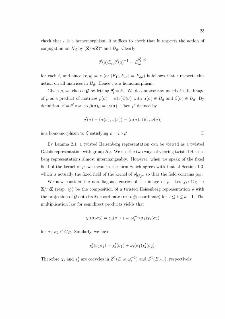
We now consider the non-diagonal entries of the image of ρ. Let χi : GE →Z/mZ (resp. χ′i) be the composition of a twisted Heisenberg representation ρ with

the projection of G onto its xi-coordinate (resp. yi-coordinate) for 2 ≤ i ≤ d−1. The

multiplication law for semidirect products yields that

χi(σ1σ2) = χi(σ1) + ω1ω−1i (σ1)χi(σ2)

for σ1, σ2 ∈ GE . Similarly, we have

χ′i(σ1σ2) = χ′i(σ1) + ωi(σ1)χ′i(σ2).

Therefore χi and χ′i are cocycles in Z1(E, ω1ω−1i ) and Z1(E,ωi), respectively.

24

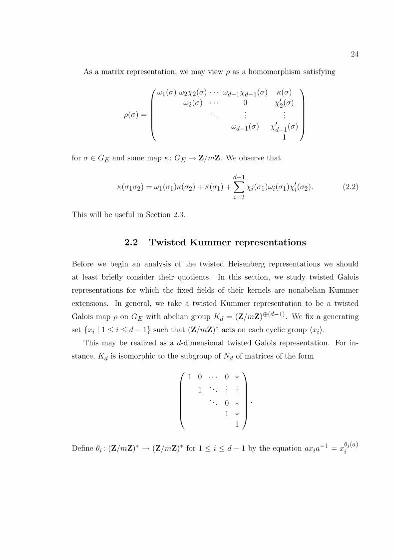
As a matrix representation, we may view ρ as a homomorphism satisfying

ρ(σ) =

ω1(σ) ω2χ2(σ) · · · ωd−1χd−1(σ) κ(σ)

ω2(σ) · · · 0 χ′2(σ). . .

......

ωd−1(σ) χ′d−1(σ)

1

for σ ∈ GE and some map κ : GE → Z/mZ. We observe that

κ(σ1σ2) = ω1(σ1)κ(σ2) + κ(σ1) +d−1∑i=2

χi(σ1)ωi(σ1)χ′i(σ2). (2.2)

This will be useful in Section 2.3.

2.2 Twisted Kummer representations

Before we begin an analysis of the twisted Heisenberg representations we should

at least briefly consider their quotients. In this section, we study twisted Galois

representations for which the fixed fields of their kernels are nonabelian Kummer

extensions. In general, we take a twisted Kummer representation to be a twisted

Galois map ρ on GE with abelian group Kd = (Z/mZ)⊕(d−1). We fix a generating

set {xi | 1 ≤ i ≤ d− 1} such that (Z/mZ)∗ acts on each cyclic group 〈xi〉.This may be realized as a d-dimensional twisted Galois representation. For in-

stance, Kd is isomorphic to the subgroup of Nd of matrices of the form1 0 · · · 0 ∗

1. . .

......

. . . 0 ∗1 ∗

1

.

Define θi : (Z/mZ)∗ → (Z/mZ)∗ for 1 ≤ i ≤ d − 1 by the equation axia−1 = x

θi(a)i

25

for a ∈ (Z/mZ)∗ and set θd = 1. Then the map

ι : Kd o (Z/mZ)∗ → PGLd(Z/mZ)

which takes (xi, 0) to the elementary unipotent matrix Eid for 1 ≤ i ≤ d − 1 and

(1, a) to the diagonal matrix with θj(a) as its jth entry realizes ρ as a twisted Galois

representation, as defined in Section 1.3. (This is not quite the form in which we are

interested in considering them with regard to twisted Heisenberg representations.)

Assume we are given a (d−1)-dimensional twisted Kummer representation ρ with

group Kd/〈xd〉, and fix a character ψ : GE → (Z/mZ)∗ yielding the action of GE on

〈xd〉 in Kd. Let L denote the fixed field of the kernel of ρ|GF.

Lemma 2.2. An element a ∈ Lψ which is not an lth power for any l dividing m

provides a lifting of ρ to a twisted Kummer representation with group Kd if and only

if the projection of a to [L×/L×m(ψ)]L/E is in the image of the restriction map from

H1(E,ψ).

Proof. Note that

Kd∼= Kd/〈xd〉 ⊕ 〈xd〉 ∼= GL/F ⊕ 〈xd〉.

Hence the map ρ will lift to a d-dimensional twisted Kummer representation as above

if and only if a ∈ Lψ is such that both TraF a = 0 and ResF TraE a = 0 by Lemma

1.9. That TraF a = 0 means exactly that a is in the image of restriction and so

comes from an element of Fψ. Given this, that ResF TraE a = 0 means exactly that

TraE a = 0, so a comes from an element of H1(E,ψ).

Remark. In order for an element a ∈ Fψ to provide a lifting, it must satisfy that a is

not an lth power in L×. That is, a should be linearly independent from the elements

b1, . . . , bd−2 for which L = K(m√b1, . . . , m

√bd−2). (The elements b1 through bd−2 can

themselves be chosen as in Lemma 2.2 with the appropriate twists.) The results of

Section 3.1 will provide conditions under which Lemma 2.2 holds.

26

2.3 Cup product

Assume we are given a twisted Galois map ρ : GE → G/Zd with group Hd/Zd. This

is a twisted Kummer representation, as defined in Section 2.2. We consider the

question of when ρ lifts to a twisted Heisenberg representation. The action of G/Zdon Zd by conjugation induces an action of GE on Zd factoring through GF/E . Hence

Zd∼= Z/mZ(ω1) under this action. For 2 ≤ i ≤ d − 1, we have as in Section 2.1

cocycles χi (resp. χ′i) coming from projection of ρ to the xi-coordinate (resp. yi) of

G.

Consider the classes of the cup products [χi ∪ χ′i] ∈ H2(E, ω1). The following

proposition tells us that the sum of these classes is the obstruction to lifting ρ, as

described in Section 1.2.

Proposition 2.3. Let ∆ be the “map” associated to the group GE and the sequence

0→ Zd → G → G/Zd → 1

as in Section 1.2. Then we have

∆(ρ) =d−1∑i=2

[χi ∪ χ′i] ∈ H2(E,ω1).

Proof. We can view ρ as a homomorphism into Bd/Zd chosen such that every matrix

(modulo its upper right hand corner) in its image has a 1 in its lower right hand

corner. We lift ρ to a map g : GE → Bd via the map taking a matrix modulo its

upper right hand corner to a matrix with a zero in its upper right hand corner. Then

by the definition given in (1.8) we have that ∆(ρ) is the class of the cocycle taking a

pair (σ1, σ2) to g(σ1)g(σ2)g(σ1σ2)−1 in Z/mZ(ψ).

27

We compute this cocycle. First, letting σ = σ1σ2, we see that

g(σ1)g(σ2) =

ω1(σ) ω2χ2(σ) · · · ωd−1χd−1(σ)

∑d−1i=2 ωiχi(σ1)χ′i(σ2)

ω2(σ) · · · 0 χ′2(σ). . .

......

ωd−1(σ) χ′d−1(σ)

1

.

Now g(σ1σ2) is the same matrix but with a zero in its upper right hand corner and

multiplication of it by z ∈ Zd just changes its upper right hand corner to (that of) z.

Hence, our cocycle is defined by

(σ1, σ2) 7→d−1∑i=2

χi(σ1)ωi(σ1)χ′i(σ2).

On the other hand, we have by definition of the cup product [12, p. 117] that

χi ∪ χ′i(σ1, σ2) = χi(σ1)ωi(σ1)χ′i(σ2)

as well.

2.4 Three-dimensional Heisenberg representations

In this section we let d = 3 and assume that E = F contains µm. In this case, we

have just the two cocycles χ = χ2 and χ′ = χ′2, which are in fact characters. The

obstruction to lifting the two-dimensional Kummer representation ρ as in Section 2.3

is given by the cup product [χ ∪ χ′]. Via our fixed choice of isomorphism in Section

1.1, any character χ has an associated element a ∈ F×, well-defined up to mth powers

in F×, such that

χ(τ) = Indτ(m√a)

m√a

for all τ ∈ GF . The cup product can then be viewed as a homomorphism

(· , ·) : F× × F× → H2(F,Z/mZ),

28

which is the norm residue symbol. This means that if χ and χ′ have representative

elements a and b in F× then [χ ∪ χ′] = (a, b).

By Kummer theory, the fixed field of the kernel of the representation ρ is L =

F (m√a,m√b). Let K = F (m

√a) and K ′ = F (m√b). Let τ ∈ GL/K′

∼= GK/F be the

generator satisfying τ(m√a) = ζmm

√a (i.e., χ(τ) = 1). Similarly, let τ ′ ∈ GL/K

∼=GK′/F be such that τ ′(m

√b) = ζm

m√b. The norm residue symbol (a, b) is trivial if

and only if b ∈ NK/FK× [15, XIV.2]. So ρ will lift if and only if b = NK/Fβ for

some β ∈ K×.

Lemma 2.4. Let β ∈ K× be such that NK/F (β) ∈ K ′×m. Set

c =m−1∏j=0

τ j(β)j . (2.3)

Then we have ν(c) ≡ c mod L×m for all ν ∈ GL/F .

Proof. As c ∈ K, it suffices to show that c is fixed by τ up to mth powers in L×.

Note that

τ(c) =m−1∏j=0

τ j+1(β)j = NK/F (β)−1m−1∏j=0

τ j+1(β)j+1 = cβm

NK/F (β). (2.4)

Hence τ(c) ≡ c mod L×m.

We now explicitly describe the solution to the embedding problem given by the

field K, homomorphism ρ and surjection H3 � Z/mZ⊕ Z/mZ.

Theorem 2.5. Let β ∈ K× be such that b = NK/F (β) and define c as in (2.3). Then

we have that ρ lifts to a Heisenberg representation ρ with

ρ(ν) = Indν(m√c)

m√c

for ν ∈ GL. Furthermore, c is unique up to multiplication by an element of F×L×m.

29

Proof. Note that τ(c) = cb−1βm by (2.4). As τ ′(c) = c, we have for any extension of

τ ′ to K(m√c) that τ ′m(m

√c) = m

√c. Then same holds for τ , as

τm(m√c) = m√cNK/F (β)b−1 = m√c.

To see that Tra c has order m, we observe that

[τ, τ ′](m√c) = ζmm√c (2.5)

as τ ′(m√b) = ζm(m

√b) and τ ′ fixes K. The class of Heisenberg extension L(m

√c)/L

given by Tra c is now seen to be equal to δ(ρ), as defined in Section 1.2, as (2.5)

implies that ρ([τ, τ ′]) = z and we are given ρ(τ) = x1 and ρ(τ ′) = y1. The rest

follows immediately from Proposition 1.8.

2.5 Three-dimensional twisted Heisenberg representations

In this section we remove the assumption that E contains the mth roots of unity. We

start with ρ as in Section 2.3 in the case d = 3 and assume a lifting exists, which

means by Proposition 2.3 exactly that [χ ∪ χ′] = 0 for the two off-diagonal cocycles.

The two cocycles χ and χ′ restricted to the Galois group of F = E(ζm) now have

elements a ∈ Fω1ω−12 and b ∈ Fω2 associated to them. We let K, K ′ and L be as

before. Furthermore, since the restriction from E to F satisfies

Res [χ ∪ χ′] = Res [χ] ∪ Res [χ′] = (a, b),

we have that (a, b) = 0.

Theorem 2.5 yields the following proposition for the “twisted” case.

Proposition 2.6. Let β ∈ K× be such that NK/Fβ = b. Then there exists an

element e ∈ F× such that, setting

c = em−1∏j=0

τ j(β)j ,

30

the map ρ lifts to a twisted Heisenberg representation ρ for which ρ|GLis the character

of order m associated to c.

Proof. Let c′ =∏mi=1 τ

i(β)i. By Theorem 2.5, we have that Tra c′ provides a lifting

of ρ|GFto a Heisenberg representation and is unique up to an element of F×L×m

doing so. As ρ lifts by assumption, we conclude by Proposition 1.8 that there is some

e ∈ F× for which c = c′e satisfies Tra c = δρ and providing the desired lifting.

Remark. Unfortunately, Proposition 2.6 does not tell us exactly what the element e,

and therefore c, can be. In general, e will be determined up to multiplication by any

element coming from image of the restriction

Res : H1(E,ψ)→ H1(L, ψ)L/E .

We shall describe this image in more detail in Chapter 3.

One question that arises is that of the existence of a good choice of β such that e

is allowed to be 1. In the following proposition, we give sufficient conditions for this

to be true.

Proposition 2.7. Let E′ be an extension of F with GK/E′∼= GF/E by restriction.

Assume there exists β ∈ (K/E′)ω2 with NK/F (β) = b. Then

c =m−1∏j=0

τ j(β)j

satisfies c ∈ Lω1. If ResF ◦TraE c = 0, then ρ lifts to a twisted Heisenberg represen-

tation which restricts to the character of order m associated to c on GL.

Proof. Let c be as in the statement of the proposition. For σ ∈ GF/E , which we

extend to an element of GK/E′ , we have

σ(c) =m−1∏j=0

στ j(β)j =m−1∏j=0

τ jω1(σ)ω2(σ)−1σ(β)j . (2.6)

31

Working in L×/L×m, we see that (2.6) becomes

σ(c) =m−1∏j=0

τ jω1(σ)ω2(σ)−1(β)jω2(σ)−1ω(σ) =

m−1∏j=0

τ j(β)jω(σ)ω1(σ)−1= cω(σ)ω1(σ)−1

.

Hence c ∈ Lω1 .

By Proposition 2.5 we have TraF c = δ(ρ|GF). The last statement now follows

immediately from Proposition 1.9.

In Chapter 3, we shall see that an element β as in Proposition 2.7 can often be

found in the case of local fields.

2.6 Twisted Heisenberg representations

We now let d ≥ 3 be arbitrary. Again we assume we are given a twisted Kummer

representation ρ : GE → G/Zd. To each character χi (resp. χ′i) with 2 ≤ i ≤ d−1, we

have an associated element ai (resp. bi). As we saw in Proposition 2.3, the condition

for a lifting to exist is that the sum of cup products∑d−1i=2 [χi ∪ χ′i] be zero. Via

restriction, this forces the corresponding fact on norm residue symbols over F that

d−1∑i=2

(ai, bi) = 0.

Let Ki = F (m√ai) and K ′i = F (m

√bi) for each i. We let L denote the fixed field of ρ,

which is the compositum of the fields Li = KiK′i.

We begin with some interesting observations.

Remark. As Hd is a metabelian group satisfying the exact sequence (2.1), we have by

[22, p. 29] an exact sequence

0→ Ext(2d−2⊕

Z/mZ,Z/mZ)→ H2(L/F,Z/mZ)

→ Hom(2d−2⊕

Z/mZ ∧2d−2⊕

Z/mZ,Z/mZ)→ 0.

32

The first term represents the extensions with trivial commutators but relations xmi =

zdi and ymi = zei . The last term is the group of possible commutator pairings and

represents the possible relations [xi, xj ] = zfij (i 6= j), [yi, yj ] = zgij (i 6= j) and

[xi, yj ] = zhij . We then have that

H2(L/F,Z/mZ) ∼= Z/mZ⊕(d−2)(2d−3)

with each summand representing one of the invariants di, ei, fij , gij and hij and

adding appropriately.

The group GE acts on each of above summands by multiplication by the twist

determined by the twists on xi and yi for each i. Thus, it is quite easy to compute the

group H2(L/F, ψ)F/E explicitly. One could then use the corresponding Hochschild-

Serre spectral sequence to compare this to the group H2(L/E, ψ).

In the case that each of the individual cup products [χi ∪ χ′i] is trivial, we can

give a nice description of the lifting ρ by describing the element c ∈ L× such that ρ

is the character of order m associated to c on GL.

Proposition 2.8. Assume [χi ∪ χ′i] = 0 for each 2 ≤ i ≤ d− 1. Let βi ∈ Ki be such

that NKi/F(βi) = bi and set

ci =m−1∏j=0

τji (βi)

j .

Then there exists e ∈ F× for which

c = e

d−1∏i=2

ci

satisfies c ∈ Lω1 and such that ρ lifts to ρ with restriction to GL equal the character

of order m associated to c.

33

Proof. We have by functoriality of the transgression a commutative diagram

⊕d−1i=2 (Li

×/Li×pn

)Li/FTra //

Res��

⊕d−1i=2 H

2(Li/F,Z/mZ)

Inf��

(L×/L×pn

)L/FTra // H2(L/F,Z/mZ).

(2.7)

If we let ρi denote the projection of ρ|GFonto the subgroup of Hd generated by

xi and yi and isomorphic to H3, then ρi is a Heisenberg representation of dimension

3. We have by Proposition 2.5 an equality of classes

TraF ci = δ(ρi) ∈ H2(Li/F, ω1).

This tells us that Inf TraF ci is the class of the extension satisfying [xi, yi] = z and

with all other commutators and all mth powers of the generators trivial.

Furthermore, we have by (2.7) that

TraF c =d−1∑i=2

Inf (TraF ci)

That TraF c = δ(ρ|GF) is now just the fact that the sum of factor sets yields exactly

the commutator relations for the given Heisenberg extension. Finally, the existence

of e follows from the existence of a lifting as in Proposition 2.6.

Remark. The obvious generalization of Proposition 2.7 to d ≥ 3 holds as well: that

is, with the requirement that βi ∈ (Ki/E′i)ωi for a proper choice of field E′i.

CHAPTER 3

LOCAL FIELDS

3.1 The Hochschild-Serre spectral sequence

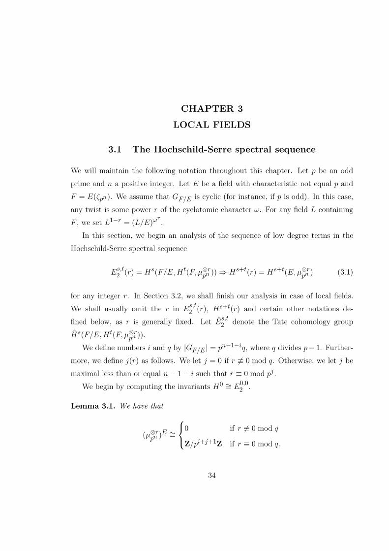
We will maintain the following notation throughout this chapter. Let p be an odd

prime and n a positive integer. Let E be a field with characteristic not equal p and

F = E(ζpn). We assume that GF/E is cyclic (for instance, if p is odd). In this case,

any twist is some power r of the cyclotomic character ω. For any field L containing

F , we set L1−r = (L/E)ωr.

In this section, we begin an analysis of the sequence of low degree terms in the

Hochschild-Serre spectral sequence

Es,t2 (r) = Hs(F/E,Ht(F, µ⊗rpn ))⇒ Hs+t(r) = Hs+t(E, µ⊗rpn ) (3.1)

for any integer r. In Section 3.2, we shall finish our analysis in case of local fields.

We shall usually omit the r in Es,t2 (r), Hs+t(r) and certain other notations de-

fined below, as r is generally fixed. Let Es,t2 denote the Tate cohomology group

Hs(F/E,Ht(F, µ⊗rpn )).

We define numbers i and q by |GF/E | = pn−1−iq, where q divides p− 1. Further-

more, we define j(r) as follows. We let j = 0 if r 6≡ 0 mod q. Otherwise, we let j be

maximal less than or equal n− 1− i such that r ≡ 0 mod pj .

We begin by computing the invariants H0 ∼= E0,02 .

Lemma 3.1. We have that

(µ⊗rpn )E ∼=

0 if r 6≡ 0 mod q

Z/pi+j+1Z if r ≡ 0 mod q.

34

35

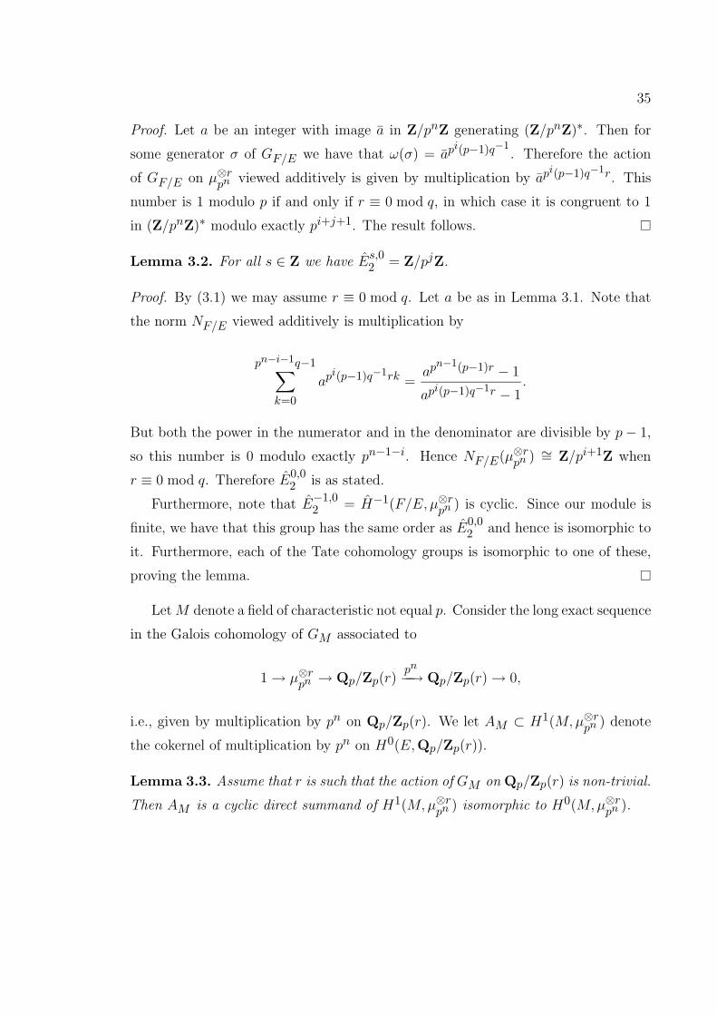
Proof. Let a be an integer with image a in Z/pnZ generating (Z/pnZ)∗. Then for

some generator σ of GF/E we have that ω(σ) = api(p−1)q−1

. Therefore the action

of GF/E on µ⊗rpn viewed additively is given by multiplication by api(p−1)q−1r. This

number is 1 modulo p if and only if r ≡ 0 mod q, in which case it is congruent to 1

in (Z/pnZ)∗ modulo exactly pi+j+1. The result follows.

Lemma 3.2. For all s ∈ Z we have Es,02 = Z/pjZ.

Proof. By (3.1) we may assume r ≡ 0 mod q. Let a be as in Lemma 3.1. Note that

the norm NF/E viewed additively is multiplication by

pn−i−1q−1∑k=0

api(p−1)q−1rk =

apn−1(p−1)r − 1

api(p−1)q−1r − 1

.

But both the power in the numerator and in the denominator are divisible by p− 1,

so this number is 0 modulo exactly pn−1−i. Hence NF/E(µ⊗rpn ) ∼= Z/pi+1Z when

r ≡ 0 mod q. Therefore E0,02 is as stated.

Furthermore, note that E−1,02 = H−1(F/E, µ⊗rpn ) is cyclic. Since our module is

finite, we have that this group has the same order as E0,02 and hence is isomorphic to

it. Furthermore, each of the Tate cohomology groups is isomorphic to one of these,

proving the lemma.

LetM denote a field of characteristic not equal p. Consider the long exact sequence

in the Galois cohomology of GM associated to

1→ µ⊗rpn → Qp/Zp(r)pn−−→ Qp/Zp(r)→ 0,

i.e., given by multiplication by pn on Qp/Zp(r). We let AM ⊂ H1(M,µ⊗rpn ) denote

the cokernel of multiplication by pn on H0(E,Qp/Zp(r)).

Lemma 3.3. Assume that r is such that the action of GM on Qp/Zp(r) is non-trivial.

Then AM is a cyclic direct summand of H1(M,µ⊗rpn ) isomorphic to H0(M,µ⊗rpn ).

36

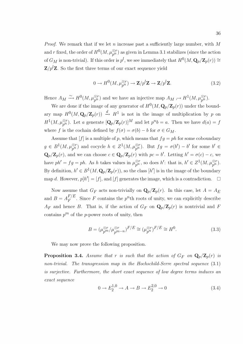
Proof. We remark that if we let n increase past a sufficiently large number, with M

and r fixed, the order of H0(M,µ⊗rpn ) as given in Lemma 3.1 stabilizes (since the action

of GM is non-trivial). If this order is pl, we see immediately that H0(M,Qp/Zp(r)) ∼=Z/plZ. So the first three terms of our exact sequence yield

0→ H0(M,µ⊗rpn )→ Z/plZ→ Z/plZ. (3.2)

Hence AM∼−→ H0(M,µ⊗rpn ) and we have an injective map AM ↪→ H1(M,µ⊗rpn ).

We are done if the image of any generator of H0(M,Qp/Zp(r)) under the bound-

ary map H0(M,Qp/Zp(r))d−→ H1 is not in the image of multiplication by p on

H1(M,µ⊗rpn ). Let a generate [Qp/Zp(r)]M and let pnb = a. Then we have d(a) = f

where f is the cochain defined by f(σ) = σ(b)− b for σ ∈ GM .

Assume that [f ] is a multiple of p, which means that fg = ph for some coboundary

g ∈ B1(M,µ⊗rpn ) and cocycle h ∈ Z1(M,µ⊗rpn ). But fg = σ(b′) − b′ for some b′ ∈Qp/Zp(r), and we can choose c ∈ Qp/Zp(r) with pc = b′. Letting h′ = σ(c)− c, we

have ph′ = fg = ph. As h takes values in µ⊗rpn , so does h′: that is, h′ ∈ Z1(M,µ⊗rpn ).

By definition, h′ ∈ B1(M,Qp/Zp(r)), so the class [h′] is in the image of the boundary

map d. However, p[h′] = [f ], and [f ] generates the image, which is a contradiction.

Now assume that GF acts non-trivially on Qp/Zp(r). In this case, let A = AE

and B = AF/EF . Since F contains the pnth roots of unity, we can explicitly describe

AF and hence B. That is, if the action of GF on Qp/Zp(r) is nontrivial and F

contains pm of the p-power roots of unity, then

B = (µ⊗rpm/µ⊗rpm−n)F/E ∼= (µ⊗rpn )F/E ∼= H0. (3.3)

We may now prove the following proposition.

Proposition 3.4. Assume that r is such that the action of GF on Qp/Zp(r) is

non-trivial. The transgression map in the Hochschild-Serre spectral sequence (3.1)

is surjective. Furthermore, the short exact sequence of low degree terms induces an

exact sequence

0→ E1,02 → A→ B → E

2,02 → 0 (3.4)

37

where A and B are defined as above and are cyclic direct summands of the respective

groups H1 and E0,12 .

Proof. We may assume r ∼= 0 mod q. Using Lemma 3.2, we know that E0,12 fits into

the exact sequence of low degree terms

0→ Z/pjZ→ H1 → E0,12 → Z/pjZ. (3.5)

By Lemma 3.3, the group H1 has a summand A ∼= Z/pkZ which is the kernel of

the map H1 → H1(E,Qp/Zp(r)). Any cocycle f with class in H1 coming from E1,02

by inflation is uniquely described by its value on σ ∈ GE with σ|F generating GF/E .

Since the action of GE on Qp/Zp(r) is non-trivial, we have necessarily f(σ) = σ(a)−afor some a ∈ Qp/Zp(r), which means that f is in A. Hence E

1,02 maps to A inside

H1. Furthermore, as restriction commutes with boundary maps, A maps into B

under restriction.

By equation (3.3) and Lemma 3.1, B and A are isomorphic. We therefore have

that the exact sequence (3.5) has the form of the sequence (3.4) of the Proposition.

Let A′ denote a complement of A in H1 and set B′ = Res(A′). Since the kernel of

Res is contained in A, we have B ∩ B′ = 0. And since the cokernel of Res is the

cokernel of Res on B, we have E0,12∼= B ⊕B′.

Remark. The transgression map need not be surjective when the action of GF on

Qp/Zp(r) is trivial. For instance, in the case pn = 4, E = R, F = C and r = 1 we

have that H1(C, µ4) = 0 while H2(C/R, µ4) ∼= Z/2Z.

Let F denote the maximal cyclotomic extension of F by p-power roots of 1 (and

therefore also of E). Note that if the action of GF on Qp/Zp(r) is trivial, then either

F = F or r = 0. Under the assumption that r = 0 and F /F is infinite, we set

A = H1(F /E,Z/pnZ) and B = H1(F /F,Z/pnZ).

Proposition 3.5. Assume that r = 0 and F /F is infinite. The transgression map

in the Hochschild-Serre spectral sequence (3.1) is surjective. Furthermore, the short

38

exact sequence of low degree terms induces an exact sequence of summands

0→ E1,02 → A→ B → E

2,02 → 0. (3.6)

Furthermore, A and B are both isomorphic to Z/pnZ.

Proof. With F1 = E(ζp), note that GF1/Ehas order prime to p. Hence, A is isomor-

phic to H1(F /F1,Z/pnZ). Both G

F /F1and G

F /Fare infinite groups injecting into

the procyclic group Zp, and are thereby isomorphic to it. The last statement follows.

The exact sequence (3.6) is just the sequence of low degree terms in the corre-

sponding Hochschild-Serre spectral sequence. The surjectivity of the transgression is

forced by the equality of the orders of A and B. Since H1 and E0,12 are killed by pn,

the groups A and B are summands.

Remark. We now comment on the application of Propositions 3.4 and 3.5 to the results

of Chapter 2. In these propositions, we describe, in their respective situations, exact

sequences of the form (3.6) which are split off as summands of the exact sequence

(3.5). In these cases, there exist complements A′ and B′ to the subgroups A and B

of H1 and E0,12 , respectively, which are mapped isomorphically to each other via the

restriction map.

Recall that in Lemma 2.2 we give a characterization of the elements of F× which

provide a lifting of a (d − 1)-dimensional twisted Kummer representation ρ to a d-

dimensional twisted Kummer representation with GE acting by ωr on 〈xd〉. The set

X of such elements can be written

X = {x ∈ F 1−r | x /∈ 〈x2, . . . , xd−1〉F×p, x /∈ im Res},

where x denotes the image of x in F×/F×pn

and Res is the restriction from E to F .

In the case j ≥ 1, the set X can be described as

X = {x ∈ F 1−r | x = yz, y ∈ B′, z ∈ B, zpi+1

= 1}.

(Note that the group of p-power roots of unity in F 1−r projects onto B.) In the case

that j = 0, all non-pth powers of L× in F 1−r will yield a lifting.

39

Furthermore, in Proposition 2.6 and Proposition 2.8 we have that the elements

e providing the freedom in the choice of the element c which yields the lifting via

transgression are those elements of F 1−r which, modulo F 1−r ∩L×pn , are contained

in the image of the restriction ResF from E to F . Note that multiplication by

elements of F 1−r ∩ L×pn (i.e., with trivial image in [L×/L×pn

(r − 1)]L/E) will not

change the lifting. These are the elements with projections to [F×/F×pn

(r− 1)]F/E

contained in the group of order p2n(d−2) generated by the images of the ai and bi

with 2 ≤ i ≤ d − 1. The elements in the image of ResF are given as the product of

any element in B′ and any elements of order dividing pi+1 in B.

3.2 The spectral sequence for local fields

We maintain the notation of the Section 3.1, restricting in this and future sections

to the case that E is a local field over Qp. In addition, we define j′(r) to be 0 if

r 6≡ 1 mod q and the maximal integer such that r ≡ 1 mod pj′

otherwise. We remark

that at least one of j and j′ is zero.

We begin with the following easy corollary of Lemma 3.1.

Lemma 3.6. We have that

H2 ∼=

0 if r 6≡ 1 mod q

Z/pi+j′+1Z if r ≡ 1 mod q.

Proof. Via the duality induced by the cup product [12, p. 170], we have that H2(r) ∼=H0(1− r), so we apply Lemma 3.1.

From this we can obtain the Tate cohomology groups.

Lemma 3.7. For all s ∈ Z we have Es,22 = Z/pj

′Z.

Proof. We first take r = 1. Note that H2(F, µpn) is the kernel of multiplication by pn

on the Brauer group Br(F ) of F . By Hochschild-Serre, we have the exact sequence

0→ H2(F/E, F×)→ Br(E)→ Br(F )F/E → 0,

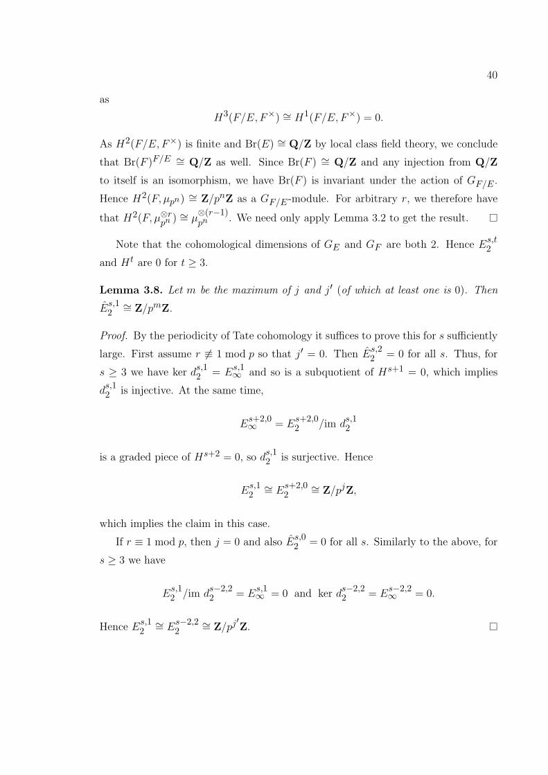
40

as

H3(F/E, F×) ∼= H1(F/E, F×) = 0.

As H2(F/E, F×) is finite and Br(E) ∼= Q/Z by local class field theory, we conclude

that Br(F )F/E ∼= Q/Z as well. Since Br(F ) ∼= Q/Z and any injection from Q/Z

to itself is an isomorphism, we have Br(F ) is invariant under the action of GF/E .

Hence H2(F, µpn) ∼= Z/pnZ as a GF/E-module. For arbitrary r, we therefore have

that H2(F, µ⊗rpn ) ∼= µ⊗(r−1)pn . We need only apply Lemma 3.2 to get the result.

Note that the cohomological dimensions of GE and GF are both 2. Hence Es,t2

and Ht are 0 for t ≥ 3.

Lemma 3.8. Let m be the maximum of j and j′ (of which at least one is 0). Then

Es,12∼= Z/pmZ.

Proof. By the periodicity of Tate cohomology it suffices to prove this for s sufficiently

large. First assume r 6≡ 1 mod p so that j′ = 0. Then Es,22 = 0 for all s. Thus, for

s ≥ 3 we have ker ds,12 = E

s,1∞ and so is a subquotient of Hs+1 = 0, which implies

ds,12 is injective. At the same time,

Es+2,0∞ = E

s+2,02 /im d

s,12

is a graded piece of Hs+2 = 0, so ds,12 is surjective. Hence

Es,12∼= E

s+2,02

∼= Z/pjZ,

which implies the claim in this case.

If r ≡ 1 mod p, then j = 0 and also Es,02 = 0 for all s. Similarly to the above, for

s ≥ 3 we have

Es,12 /im d

s−2,22 = E

s,1∞ = 0 and ker d

s−2,22 = E

s−2,2∞ = 0.

Hence Es,12∼= E

s−2,22

∼= Z/pj′Z.

41

Let us define numbers k(r) and k′(r) by #H0 = pk and #H2 = pk′. These

numbers are explicitly given in Lemmas 3.1 and 3.9. We now determine H1.

Proposition 3.9. We have that

H1 = Z/pkZ⊕ Z/pk′Z⊕ (Z/pnZ)⊕[E:Qp].

Proof. Since E is a finite extension of Qp, if the action of GE on Qp/Zp(r) is trivial,

then r = 0. In this case, we may use the duality induced by the cup product and

Kummer theory to say that

H1(E,Z/pnZ) ∼= H1(E, µpn) ∼= E×/E×pn.

The proposition then follows in this case, and in the case r = 1, from the structure

theory of the multiplicative group of a local field. That is, the multiplicative group

is isomorphic to a direct sum

E× ∼= µ⊕ Z⊕ Z⊕[E:Qp]p .

where µ denotes the group of roots of unity in E and note that µ ∼= H0(E, µpn).

We may now assume r 6= 0, 1, in which case the orders of H0 and H2 both stabilize

as n is increases. As in Lemma 3.3, we use the long exact sequence associated to

1→ µ⊗rpn → Qp/Zp(r)→ Qp/Zp(r)→ 0

and we have that A = AE∼= Z/pkZ is a direct summand of H1.

Since the cohomological dimension of GE is 2, the long exact sequence ends with

H2 → H2(E,Qp/Zp(r))pn−−→ H2(E,Qp/Zp(r))→ 0. (3.7)

The p-torsion group H2(E,Qp/Zp(r)) is therefore p-divisible. As the order of H2

stabilizes for n sufficiently large, the leftmost arrow must be zero for such n. But

this means multiplication by p is an isomorphism on H2(E,Qp/Zp(r)), which forces

H2(E,Qp/Zp(r)) to be zero.

42

Using equation (3.2), we therefore have an exact sequence

0→ Z/pkZ→ H1 → H1(E,Qp/Zp(r))pn−−→ H1(E,Qp/Zp(r))→ Z/pk

′Z→ 0.

(3.8)

Since the order of H2 stabilizes, we conclude from (3.8) that H1(E,Qp/Zp(r)) is a

direct sum of a cyclic summand Z/pl′Z and a divisible p-torsion group. Hence our

exact sequence (3.8) reduces to

0→ Z/pkZ→ H1 → (Z/pnZ)⊕i ⊕ Z/pk′Z→ 0 (3.9)

for some number i. The Euler-Poincare characteristic of µ⊗rpn as a GE-module is

|#µ⊗rpn |E = p−n[E:Qp], where | · |E is the absolute value on E [12, p. 171]. Hence the

order of H1(E, µ⊗rpn ) is pk+k′+n[E:Qp]. That is, i = [E : Qp].

Finally, we determine the remaining term in the spectral sequence.

Proposition 3.10. Let k be such that the order of H0 is pk and k′ be such that the

order of H2 is pk′. Then

E0,12 = Z/pkZ⊕ Z/pk

′Z⊕ (Z/pnZ)⊕[E:Qp].

Proof. For r 6= 0 we refer to Proposition 3.4. In the case r = 0, we are in the situation

of Lemma 3.5. In either case, we have by Proposition 3.9 that since the groups A and

B of Section 3.1 are direct summands, restriction induces an isomorphism between

complements of these groups. The complement of A is isomorphic to Z/pk′Z ⊕

Z/pnZ[E : Qp] and B ∼= Z/pkZ, so the result follows.

Remark. The groups A′ and B′ in the remarks of Section 3.1 are both isomorphic

to Z/pk′Z ⊕ Z/pnZ[E : Qp]. This allows for an exact count of the number of ele-

ments (modulo pnth powers) providing liftings of twisted Kummer representations to

higher-dimensional twisted Kummer representations or to twisted Heisenberg repre-

sentations.

43

3.3 Twisted Heisenberg representations

Let ∆ be the subgroup of GF/E of order q. Let F× denote the Zp-completion of F×.

The action of ∆ on F× is semisimple, hence F× decomposes into a direct sum of

eigenspaces for the powers of the cyclotomic character on ∆. We let Dr denote the

eigenspace consisting of x ∈ F× such that

σ(x) = xδr(σ),

where δ : ∆→ Z∗p is the character which reduces to ω|∆ under composition with the

surjection Z∗p � (Z/pZ)∗.

Lemma 3.11. The pairing

Ds ×Dt → µpn

induced by the Hilbert norm residue symbol is trivial unless t ≡ 1 − s mod q and

nondegenerate otherwise.

Proof. Let us evaluate (as, at) with as ∈ Ds and at ∈ Dt. Let i = δ(σ) for a generator

σ of ∆. Then we have

(as, at) = σ(as, at)i−1

.

By Galois equivariance of the norm residue symbol, the last term equals

(σ(as), σ(at))i−1

= (ais

s , aitt )i−1

= (as, at)is+t−1

.

Hence either is+t−1 ≡ 1 mod p or (as, at) = 1. However, as i has order dividing

p − 1, the former condition is exactly that is+t−1 ≡ 1 mod pn. This proves the first

statement and the second follows by nondegeneracy of the norm residue symbol.

Remark. Although we have not done it here, Lemma 3.11 could be used, along with

the results of Section 3.2, to gain more information on the cup product pairingH1(s)×H1(t)→ Z/mZ or on the pairing induced by the Hilbert norm residue symbol F s ×F t → µpn .

44

We now return to the situation of Section 2.5 and consider a three-dimensional

Kummer representation ρ of GE with twists given by the characters ωr−s and ωs

on the cyclic groups generated by x and y, respectively. We let K = F (pn√a) and

K ′ = F (pn√b) and L = KK ′ for a and b given as in Section 2.5. Under certain

assumptions, we can give conditions for Proposition 2.7 to hold. As in Proposition

2.7, let E′ denote a field such that GK/E′∼= GF/E via restriction.

Theorem 3.12. Assume that r 6≡ 1 mod q and j(s) = j′(s) = 0. There exists

β ∈ (K/E′)1−s with NK/F (β) = b. We have that

c =

pn−1∏i=0

τ i(β)i

satisfies c ∈ L1−r and ρ lifts to a twisted Heisenberg representation which restricts to

the character of order pn associated to c on GL. Furthermore, if j(r) = 0 then the

element c ∈ L1−r providing a lifting is unique up to multiplication by any element of

F 1−rL×pn

.

Proof. For an integer t, we define

Nt : F×/F×p

n(t− 1)→ [F×/F×p

n(t− 1)]F/E

by

Nt(X) =∏

σ∈GF/E

σ(X)ωt(σ)

for X ∈ F×/F×pn

. We also let Nt denote any lifting of Nt to a homomorphism

Nt : F× → F 1−t.

As j(s) = j′(s) = 0, we see that E0,12 (s) = 0 by Lemma 3.8. As b ∈ F 1−s, we have

therefore that b = δpnNs(γ) for some δ, γ ∈ F×. Note also that NsDi ⊂ F× ∩ F×pn

if i 6≡ 1− s mod q. Hence, we may assume γ ∈ D1−s.

Since r 6≡ 1 mod q we conclude by Lemma 3.11 that (a, γ) = 1. Hence, there

exists α ∈ K such that γ = NK/F (α). Set β = δNs(α) ∈ K1−s after extending Ns

45

to a map on K× defined in the same manner (via the identification of GF/E with

GK/E′ as in Proposition 2.7). Note that Ns commutes with NK/F . We see that

NK/F (β) = δpnNsNK/F (α) = δp

nNs(γ) = b.

As r 6≡ 1 mod q, we have that H2(r) = 0. Hence, ResF ◦TraE is the trivial map.

That ρ lifts to a twisted Heisenberg representation follows from Proposition 2.7.

The last statement follows from the remarks at the end of Section 3.1. That is,

the kernel of TraE is the image of the restriction

Res : H1(r)→ H1(L, µ⊗rpn )L/E .

If j(r) = 0 then E2,02 (r) = 0, and therefore Res factors through E

0,12 (r). Hence the

product of c and any element of F 1−r also yields a lifting.

Remark. Alternatively to assuming j(s) = j′(s) = 0, one may merely assume that

b ∈ F×pnNsF×. This should often not be necessary: i.e., that b be a twisted norm

rather than just invariant under a twisted action. Furthermore, the restriction r ≡1 mod q is clearly not always necessary, for instance when F = E.

CHAPTER 4

RAMIFICATION

4.1 Preliminaries

In this section, we prove some general lemmas on ramification numbers of local fields

which will be useful to us later. These are well-known or easy, but for convenience

we prove them here. For a Galois extension with group G, let φG and ψG be the

functions which allow one to pass between the lower and upper numberings of the

ramification groups [15, IV.3]. In particular, for a real number w ≥ −1 we have

Gw = GψG(w) and Gw = GφG(w).

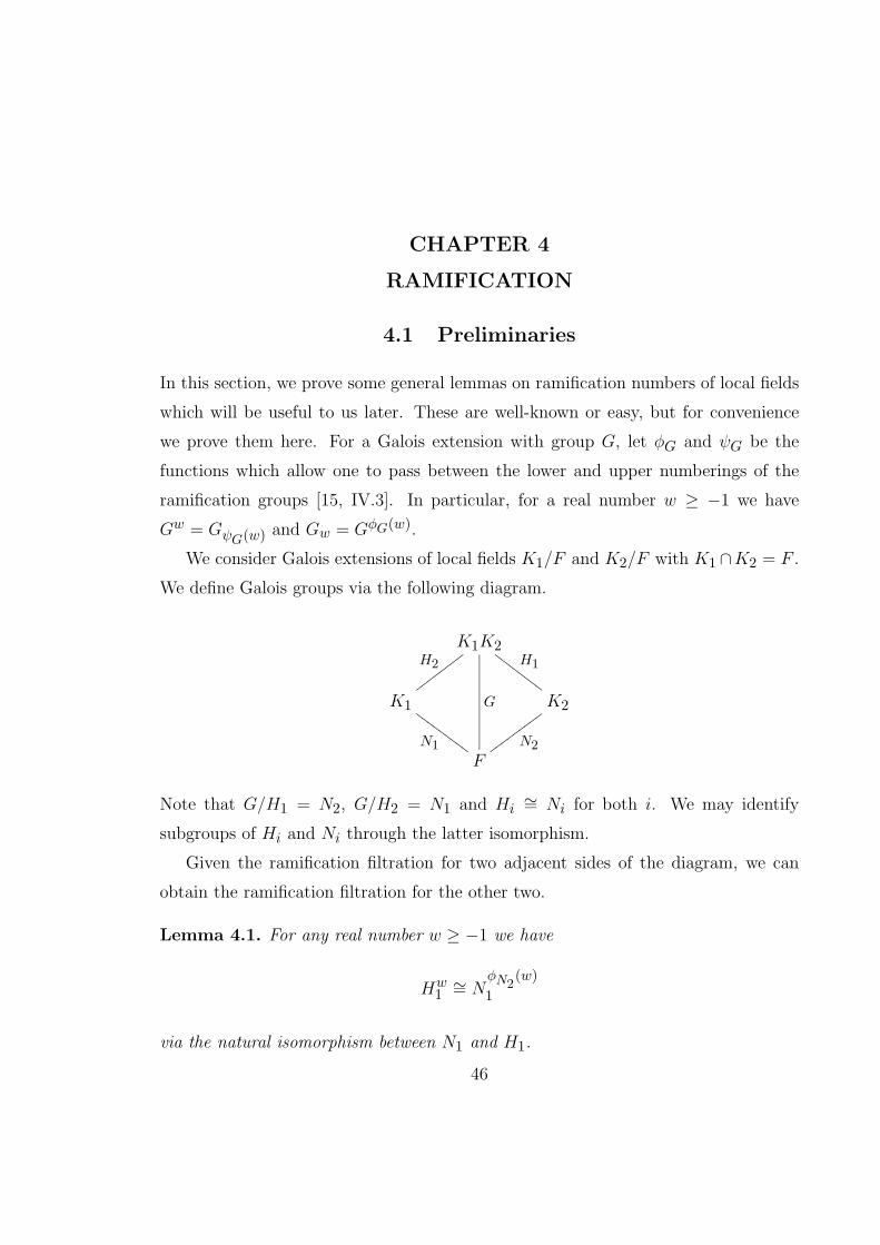
We consider Galois extensions of local fields K1/F and K2/F with K1 ∩K2 = F .

We define Galois groups via the following diagram.

K1K2

K1

H2wwwwwwww

K2

H1GGGGGGGG

FN1

GGGGGGGGG N2

wwwwwwwww

G

Note that G/H1 = N2, G/H2 = N1 and Hi ∼= Ni for both i. We may identify

subgroups of Hi and Ni through the latter isomorphism.

Given the ramification filtration for two adjacent sides of the diagram, we can

obtain the ramification filtration for the other two.

Lemma 4.1. For any real number w ≥ −1 we have

Hw1∼= N

φN2(w)

1

via the natural isomorphism between N1 and H1.

46

47

Proof. This follows from the usual properties of the ramification numberings [15,

IV.3], as we demonstrate below. We have

Hw1 = (H1)ψH1

(w) = GψH1(w) ∩H1 = G

φN2(w) ∩H1.

Using the isomorphism between H1 and N1 = G/H2, this becomes

GφN2

(w)H2/H2 = N

φN2(w)

1 .

We also have the following trivial corollary.

Corollary 4.2. For any real number w ≥ −1, we have

Nw1∼= H

ψN2(w)

1 .

Hence, a jump in the ramification filtration of K1/F occurs at a number l in the

upper numbering of if any only if a jump in the filtration of K1K2/K2 occurs at

ψN2(l).

In this chapter, p will denote an odd prime. For a local field K/Qp containing the

pnth roots of unity and a ∈ K× we denote by fn,K(a) the conductor of K(pn√a)/K

(considered as an integer) [15, XV.2], and we let ( · , · )n,K denote the pnth norm

residue symbol of K. Let Ui denote the ith unit group of K for i ≥ 1, and set U0 = U .

Then f = fn,K(a) is the smallest nonnegative integer for which (a, u)n,K = 1 for all

u ∈ Uf .

Let e denote the ramification index of K. We have the following lemma.

Lemma 4.3. If fn,K(ap) > e/(p− 1) + 1 then fn,K(a) = fn,K(ap) + e.

Proof. Let b ∈ Ue/(p−1)+1, so that the valuation of bp−1 is e more than that of b−1.

Since (ap, b)n,K = (a, bp)n,K , we conclude that fn,K(a) = fn,K(ap) + e.

48

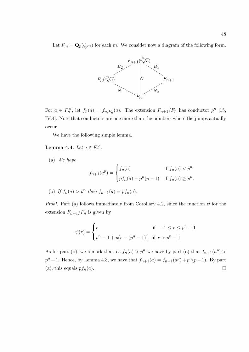
Let Fm = Qp(ζpm) for each m. We consider now a diagram of the following form.

Fn+1(pn√a)

Fn(pn√a)

H2qqqqqqqqqq

Fn+1

H1KKKKKKKKKK

Fn

N1

NNNNNNNNNNNN N2

rrrrrrrrrrr

G

For a ∈ F×n , let fn(a) = fn,Fn(a). The extension Fn+1/Fn has conductor pn [15,

IV.4]. Note that conductors are one more than the numbers where the jumps actually

occur.

We have the following simple lemma.

Lemma 4.4. Let a ∈ F×n .

(a) We have

fn+1(ap) =

fn(a) if fn(a) < pn

pfn(a)− pn(p− 1) if fn(a) ≥ pn.

(b) If fn(a) > pn then fn+1(a) = pfn(a).

Proof. Part (a) follows immediately from Corollary 4.2, since the function ψ for the

extension Fn+1/Fn is given by

ψ(r) =

r if − 1 ≤ r ≤ pn − 1

pn − 1 + p(r − (pn − 1)) if r > pn − 1.

As for part (b), we remark that, as fn(a) > pn we have by part (a) that fn+1(ap) >

pn+ 1. Hence, by Lemma 4.3, we have that fn+1(a) = fn+1(ap) +pn(p− 1). By part

(a), this equals pfn(a).

49

4.2 The multiplicative group as a module

Let F = Qp(ζpn). We may decompose GF/Qpwith p odd into a direct product of

cyclic groups ∆×Γ where ∆ has order p− 1 and Γ has order pn−1. We let F1 denote

the fixed field Qp(ζp) of Γ. We also define F×, Dr and δ as in Section 3.3. It is the

goal of this section to gain an understanding of the Zp[Γ]-module structure of Dr.

We begin with the following lemma regarding the structure of Dr.

Lemma 4.5. The eigenspace Dr has rank pn−1 +1 as a Zp-module if r ≡ 0 mod p−1

and pn−1 otherwise. If r ≡ 1 mod p − 1, then Dr has non-zero cyclic torsion and

otherwise Dr has no torsion. Furthermore, Dr has a minimal set of generators

{xt ∈ Ut − Ut+1 | t ≡ r mod p− 1, p - t, t < pn}

with one extra generator x0 of non-zero valuation when r ≡ 0 mod p − 1 and one

extra generator xpn ∈ Upn − Upn+1 when r ≡ 1 mod p− 1.

Proof. Note first that the only torsion is µpn , which is contained in D1. Consider

x ∈ Dr for some r. If x has non-zero valuation, then since σ(x) has the same valuation

as x, we must have r ≡ 0 mod p− 1. As F× is the direct sum of the Dr, there exists

x0 ∈ D0 with valuation 1. So assume that x is a unit, x ∈ Ut−Ut+1. Let λn = 1−ζpn .

Then we have

σ(λn) ≡ δ(σ)λn mod (λ2n).

So we see that

σ(x) ≡ 1 + δ(σ)t(x− 1) ≡ xδ(σ)t mod (λt+1n ).

Hence, as x ∈ Dr, we must have t ≡ r mod p− 1. Furthermore, for each such t, there

is an element xt ∈ Ut ∩Dr such that xt 6∈ Ut+1, for instance,

xt =∏σ∈∆

(1− σ(λtn))δ(σ)−t.

50

To see xt 6∈ Ut+1, note that we have

xt ≡∏σ∈∆

(1− δ(σ)tλtn)δ(σ)−t≡ (1− λtn)p−1 ≡ 1 + λtn mod (λt+1

n ).

Note that none of the elements of

X = {xt | p - t, t < pn or t = 0, pn}

can be pth powers. Furthermore, the elements of X are linearly independent in the

the pn−1(p − 1) + 2-dimensional Z/pZ-vector space F×/F×pn

. Therefore, X is a

minimal generating set of F×

as a Zp-module.

Recall that fn(x) denotes the conductor of F (pn√x)/F . We have the following easy

corollary of Lemmas 3.11 and 4.5.

Corollary 4.6. Let x ∈ Dr∩F×. Then either fn(x) ≡ 2−r mod p−1 or fn(x) = 1.

Proof. If for some s we have a unit y ∈ U1∩Ds with (x, y) 6= 1, then s ≡ 1−r mod p−1

by Lemma 3.11. By Lemma 4.5 we have that v(y − 1) ≡ 1 − r mod p − 1, where v

denotes the additive valuation on F .

Each eigenspace Dr is a Zp[Γ]-module. By Iwasawa Theory [13, §7.2], we know

that in fact Dr is a free Zp[Γ]-module of rank 1 when r 6≡ 0, 1 mod p− 1. We give a

nice proof of this result, suggested by Hendrik Lenstra.

Proposition 4.7. If r 6≡ 0, 1 mod p − 1 then Dr is a free Zp[Γ]-module of rank 1.

Otherwise Dr can be generated by two elements as a Zp[Γ]-module.

Proof. By Lemma 4.5, Dr has the correct minimal number of Zp-generators to be a

free of rank one Zp[Γ]-module when r 6≡ 0, 1 mod p − 1, but one too many for this

when r ≡ 0, 1 mod p − 1. Hence it takes at least one element to generate Dr as a

Zp[Γ]-module when r 6≡ 0, 1 mod p− 1 and at least two otherwise. In total, we must

have at least p+ 1 generators.

Consider the abelian extension L of F with norm group F×pIΓF×, where IΓ is

the augmentation ideal of Z[Γ]. Let H = NF/F1F×. By local class field theory we

51

have a Γ-module isomorphism GL/F∼= F×/F×pIΓF

×. Hence Γ acts trivially on this

GL/F by conjugation. That is, L/F1 is abelian. Furthermore,

NL/F1L× = NF/F1

(F×pIΓF×) = NF/F1

F×p = Hp.

Therefore the order of F×/F×pIΓF×, which is p to the minimal number of generators

of F× as a Zp[Γ]-module, is equal to the index [H : Hp].

But H is a subgroup of F×1 , the completion of which is a Zp-module generated

by p + 1 elements. Hence [H : Hp] ≤ pp+1. As we know that we must have at least

p+ 1 generators, we have equality and the proposition is proven.

Greither [8] has worked out explicitly the Galois module structure of F× (and in

fact for any finite unramified extension of F ). Though we shall not actually use it,

Greither’s result is useful in dealing with the “bad” cases r ≡ 0, 1 mod p − 1 in the

determination of conductors as in Section 4.4. Therefore, we state the result below

in our case, attempting to maintain a degree of notational consistency with [8].

Let Q be the Z[GF/Qp]-module with generators Π and V and the relation ∆ fixes

V . Let Q0 denote the submodule generated by U and V with U = σ(Π) − Π for

some generator σ of ∆. Let Q0,p denote the Zp-completion of Q0. Let Qp denote the

pushout Q0,p qQ0Q. Finally, let Q′ = Qp × µ where µ is the module isomorphic to

all roots of 1 in F .

Theorem 4.8 (Greither). There is an isomorphism Q′ → F× of Z[GF/Qp]-modules

taking Π to a prime element, V to 1− p, and the roots of unity to themselves.

Remark. Theorem 4.8 is obtained via specifying Theorem 3.1 of [8] to the case of a

totally ramified extension. The statement follows since Q as defined in [8] satisfies

Q×µpn ∼= Q′ and since his map β induces a split exact sequence by Step 2 of Theorem

2.9 of [8].

By taking Zp-completions, we obtain the following result.

52

Corollary 4.9. There exists a prime element π of F× such that the Zp[GF/Qp]-

submodule M of F× generated by π is free and yielding a decomposition

F× = M × µpn × 〈1− p〉Zp .

4.3 Comparison of module structure with unit filtration

Let π and M be as in Corollary 4.9, and set Mr = Dr ∩M for all r. Then Mr is

a free Zp[Γ]-module of rank 1, and for r 6≡ 0, 1 mod p − 1 we have Mr = Dr. We

choose a generator yr of Mr as a Zp[Γ]-module. We identify Mr with Zp[Γ] via the

isomorphism

Zp[Γ]∼→Mr, α 7→ yαr (4.1)

of Zp[Γ]-modules. Each subgroup arising from a unit group Vt = Ut ∩Mr with t > 0

becomes identified with an ideal of Zp[Γ] (independent of yr) and by abuse of notation

we treat them as equal. (Therefore, we may use either additive or multiplicative

notation, depending on what is most notationally convenient for the situation.) Note

that Lemma 4.5 implies that Vt = Vt+1 for t 6≡ r mod p− 1. Therefore we need only

consider t ≡ r mod p− 1.

Let γ denote a generator of Γ. We wish to determine Vt as an ideal. Note that

[Vt : Vt+p−1] is either 1 or p, and if t 6≡ 0, 1 mod p− 1 then [Vt : Vt+p−1] = p. We set

V ′t = Vt − Vt+p−1. If 2 ≤ u ≤ p − 2, then Vu = Zp[Γ] and, as Zp[Γ] is a local ring,

Vu+p−1 is the maximal ideal (p, γ − 1).

Lemma 4.10. Let xt ∈ V ′t for t ≡ r mod p − 1. If p - t, then γ(xt)/xt ∈ V ′t+p−1.

Otherwise, γ(xt)/xt ∈ Vt+2(p−1).

Proof. From the ramification groups of F/Qp in the lower numbering [15, IV.4], we

see that v(γ(π)/π − 1) = p − 1, where v is the valuation on F and π is any prime

element of F . Hence, for any x ∈ Ut with p - v(x−1), we have v(γ(x)−x) = t+p−1.

On the other hand, if p | v(x− 1) then v(γ(x)− x) > t+ p− 1. Since γ(xt)/xt ∈Mr,

the result follows.

53

Lemma 4.11. Let xt ∈ V ′t for t ≡ r mod p− 1. For j ≥ 1, we have

x(γ−1)jt ∈ Vjp.

Proof. We will show the stronger result that

x(γ−1)jt ∈ V

t+(j+[

j−qp−1

])(p−1)

, (4.2)

where [ · ] denotes the ceiling function and q denotes the smallest nonnegative integer

with q ≡ t mod p− 1. This implies the lemma since

t+(j +

[j − qp− 1

])(p− 1) ≥ t+ j(p− 1) + j − q ≥ jp.

Lemma 4.10 implies that V(γ−1)u ⊆ Vu+p−1 for all u ≡ t mod p− 1. Hence

x(γ−1)jt ∈ Vu+j(p−1). (4.3)

Furthermore, Lemma 4.10 implies that x(γ−1)qt ∈ V ′

p+(p−1)q and that a(γ−1)p−1 ∈Vu+p(p−1) for a ∈ V ′u with u ≡ t mod p− 1. Together these show that for every p− 1

applications of γ − 1 after the qth and starting with the (q + 1)st, we can add an

additional p− 1 to the subscript of V in (4.3), which yields equation (4.2).

4.4 Conductors in the metabelian case

We keep the notation of the previous section, but we now choose γ so that γ(ζpn) =

ζ1+ppn . By (1.4), we have that x ∈ F 1−r implies

γ(x) ≡ x(1+p)1−rmod F×p

n. (4.4)

Furthermore, we assume in this section that r 6≡ 0, 1 mod p − 1. We then have as

before yr ∈ Dr generating Dr as a free Zp[Γ]-module, and hence its image generates

Dr/(Dr ∩F×pn) as a free Z/pnZ[Γ]-module.

54

Let x ∈ F 1−r. Our goal in this section is the determination of the conductor of

the extension F (pn√x)/F . This is exactly the conductor of the norm residue symbol

(x, · ), where ( · , · ) denotes the pnth norm residue symbol over F .

Lemma 4.12. If x ∈ F 1−r and x 6∈ F×p, then the symbol (x, yr) is a primitive pnth

root of unity.

Proof. The nondegeneracy of the norm residue symbol as proven in Lemma 3.11

implies that (x, y) is a primitive pnth root of unity for some y ∈ Dr. But as Dr is a

free Zp[Γ]-module generated by yr, and since we have that

γ(x, yr) = (x, γ(yr))(1+p)1−r

by (4.4), this cannot happen unless (x, yr) is a primitive pnth root of unity as well.

For α ∈ Dr, we let [x, α] ∈ Z/pnZ denote the power of (x, yr) which (x, α) equals.

Lemma 4.13. Let

α = yf(γ)r

with f ∈ Zp[X]. Then

[x, α] ≡ f((1 + p)r) mod pn.

Proof. We need only show that [x, γj(yr)] = (1 + p)jr. We have

(x, γj(yr)) = γj(γ−j(x), yr) = (x(1+p)−j(1−r), yr)

(1+p)j = (x, yr)(1+p)jr .

Corollary 4.14. We have

(x, ypk(γ−1)n−k

r ) = 1

for 0 ≤ k ≤ n.

Proof. We calculate:

[x, ypk(γ−1)n−k

r ] = pk(1 + p− 1)n−k ≡ 0 mod pn.

55

Note that

Zp[Γ] ∼= Zp[X]/(Xpn−1− 1).

We shall require the following result.

Lemma 4.15. In Zp[X], the polynomial Xpn−1 − 1 is contained in the ideal

(pn−1(X − 1), pn−2(X − 1)p, . . . , (X − 1)pn−1

).

Proof. Let Y = X − 1. We need only show that

(Y + 1)pn−1− 1 ∈ (pn−1Y, pn−2Y p, . . . , Y p

n−1).

It suffices therefore to verify that if pm ≤ k < pm+1 with 0 ≤ m < n − 1 then

vp((pn−1

k

))≥ n − 1 − m, where vp denotes the p-adic valuation. We note that, in

fact,

vp((pn−1

k

))= n− 1− vp(k)

for 1 ≤ k ≤ pn−1, which implies the claim.

To determine the conductor of (x, · ), it suffices to look at two ideals of Zp[Γ]. Let

t denote the smallest nonnegative integer such that t ≡ r mod p− 1.

Lemma 4.16. The ideal Vpn−1(t+1)−1 of Dr contains an element a of the form

a = pn−1 +n−1∑k=1

dkpn−1−k(γ − 1)p

k−1(t+1)−1

with dk ∈ Zp. The ideal Vpn−1(t+1)+p−2 of Zp[Γ] is generated by pn, pn−1(γ−1) and

pn−1−k(γ − 1)pk−1(t+1) for 1 ≤ k ≤ n− 1.

Proof. We begin with the second statement. We abuse notation via the identification

(4.1) so that we can consider the unit groups additively. By Lemma 4.15, we have

56

that the ideal I of Zp[X] generated by pn−1(X − 1) and pn−1−k(X − 1)pk−1(t+1) for

1 ≤ k ≤ n− 1 contains Xpn−1 − 1. Hence the image of I in Zp[Γ] has index equal to

the index of I in Zp[X]. This is equal to p to the power of

n+t(n−1)+(p−1)(t+1)(n−2)+. . .+pn−3(p−1)(t+1) = (pn−2+. . .+p+1)(t+1)+1.

This is equal to [Zp[Γ] : Vpn−1(t+1)+p−2].

To prove the second statement, we are left only to verify the claim that I ⊆Vpn−1(t+1)+p−2. By Lemma 4.10, we see that

pn−1(γ − 1) ∈ pn−1Vt+p−1 ⊆ pn−1Vp ⊆ Vpn ⊆ Vpn−1(t+1)+p−2

as 2 ≤ t ≤ p− 2. Similarly, Lemma 4.11 yields

pn−k−1(γ−1)pk−1(t+1) ∈ pn−k−1V

pk(t+1)+p−2 ⊆ Vpn−1(t+1)+pn−k−1(p−2) ⊆ Vpn−1(t+1)+p−2.

Hence we have the claim.

For the first statement, we proceed by constructing a finite sequence of elements

which are not contained in I, the last of which is the desired element. Note that for

an element b ∈ V ′u for some u ≡ t mod p such that pb /∈ I, we have pb ∈ V ′pu since

Vpn+1 ⊆ I.

In V ′pt we have two distinct elements: p and a1 for some element a1 ∈ Zp[Γ] which

is nonzero modulo p. The latter element exists by Lemma 4.10, as (γ − 1)g ∈ V ′ptfor any g ∈ V ′

p(t+1)−1. Multiplying a1 by a constant which is nonzero modulo p if

necessary, we can insure that

p+ a1 ∈ Vpt+p−1.

Then we have p2 + pa1 ∈ Vp2(t+1)−p. In fact, the latter element is in V ′pu for some

u ≡ t mod p− 1. Therefore, we can find as above a2 6≡ 0 mod p in V ′pu such that

p2 + pa1 + a2 ∈ Vp2(t+1)−1.

57

Multiplying this by p, we have an element in Vp3(t+1)−p. Continuing on in this

fashion, we obtain an element

a = pn−1 + pn−2a1 + . . .+ an−1 ∈ Vpn−1(t+1)−1.

As a is not an element of I (by the second statement), we have in fact that

a ∈ V ′pn−1(t+1)−1

. As

(γ − 1)Vpn−1(t+1)−1 ⊆ Vpn−1(t+1)+p−2,

we have by the second statement that Vpn−1(t+1)−1 is contained in the ideal generated

by pn−1 and pn−1−k(γ− 1)pk−1(t+1)−1 for 1 ≤ k ≤ n− 1. Using this and the second

statement, it is clear that ak may be chosen to have the form dk(γ−1)pk−1(t+1)−1.

We now determine the desired conductors.

Theorem 4.17. Let r 6≡ 0, 1 mod p − 1 and let t denote the smallest nonnegative

integer with t ≡ r mod p − 1. Let x ∈ F 1−r with x 6∈ F×p. Then we have that

fm,F (x) = (t+ 1)pm−1 for any positive integer m with m ≤ n.

Proof. By Corollary 4.14, (x, y) = 1 for each generator y of Vpn−1(t+1)+p−2 listed in

Lemma 4.16. On the other hand, for the element a ∈ Zp[Γ] of Lemma 4.16, we have

[x, yar ] = [x, ypn−1

r ] = pn−1.

Noting Corollary 4.6, we see that the conductor of x is therefore ((1− ζpn)pn−1(t+1)).

Setting Fm = Qp(ζpm) and fm = fm,Fm as in Section 4.1, we now have that

fm(x) = pm−1(t+ 1). Since t+ 1 < p, Lemma 4.4a yields that

fm,F (x) = fn(xpn−m

) = fm(x),

which is as desired.

58

Remark. Although we have not written it out here, to compute the conductors for

elements fixed under a twisted action of GF/Qpin the “bad” cases r ≡ 0, 1 mod p−1,

one can use Theorem 4.8 and proceed as in this section. In fact, one can in all cases

actually determine explicit generators for each Vt as an ideal of Zp[γ], as we have

done in some specific cases in Lemma 4.16.

4.5 Ramification in a Heisenberg extension

We consider the twisted Heisenberg extension Qp(ζpn ,pn√p,p

n√1− p,pn√

cn)/Qp, where

cn =

pn∏i=1

(1− ζipnpn√p)i.

This example is fundamental as, up to multiplying cn by an element of F×, it is the

only Heisenberg extension with lower steps coming from adjoining Qp all of its pnth

roots. (In fact, our computations will show that the conductor of the top step does

not depend in this case on the choice of cn.)

Let Fn = Qp(ζpn), Kn = Fn(pn√p), K ′n = Fn(p

n√pp(1− p)) and Ln = KnK

′n.

The conductors of Kn/Fn and K ′n/Fn were computed for all n ≥ 1 in [3] (see also

[20]). By induction on n, we shall determine the conductors of K ′n(pm√c′n)/K ′n for all

m ≤ n, where c′n ∈ K ′n differs from cn by a pnth power in Kn. We shall then use

these conductors to compute the conductors of Ln(pn√cn)/Ln.

We begin with the case n = 1.

Proposition 4.18. We have f1,K′1(c′) = p2 − p+ 3.

Proof. For notational simplicity, we drop all subscript 1’s from the notation in this

proof. We have the following diagram of field extensions, in which the numbers denote

the conductors of the indicated extension. (The conductors of K/F and K ′/F are

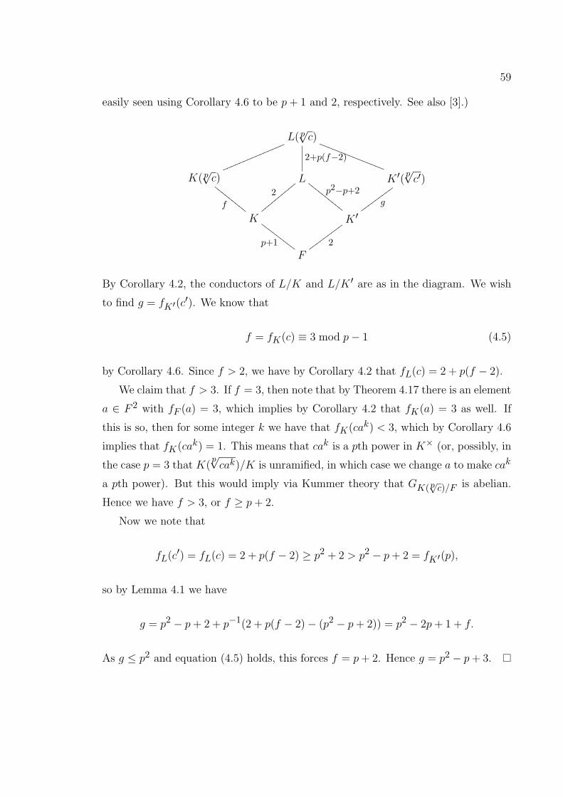
59

easily seen using Corollary 4.6 to be p+ 1 and 2, respectively. See also [3].)

L(p√c)

K(p√c)

lllllllllllllllL

2+p(f−2)

K ′(p√c′)

RRRRRRRRRRRRRRR

K

f

EEEEEEEEE

2yyyyyyyyyy

K ′

p2−p+2EEEEEEEEEE g

wwwwwwwww

Fp+1

GGGGGGGGG 2

wwwwwwwww

By Corollary 4.2, the conductors of L/K and L/K ′ are as in the diagram. We wish

to find g = fK′(c′). We know that

f = fK(c) ≡ 3 mod p− 1 (4.5)

by Corollary 4.6. Since f > 2, we have by Corollary 4.2 that fL(c) = 2 + p(f − 2).

We claim that f > 3. If f = 3, then note that by Theorem 4.17 there is an element

a ∈ F 2 with fF (a) = 3, which implies by Corollary 4.2 that fK(a) = 3 as well. If

this is so, then for some integer k we have that fK(cak) < 3, which by Corollary 4.6

implies that fK(cak) = 1. This means that cak is a pth power in K× (or, possibly, in

the case p = 3 that K(p√cak)/K is unramified, in which case we change a to make cak

a pth power). But this would imply via Kummer theory that GK(p√c)/F is abelian.

Hence we have f > 3, or f ≥ p+ 2.

Now we note that

fL(c′) = fL(c) = 2 + p(f − 2) ≥ p2 + 2 > p2 − p+ 2 = fK′(p),

so by Lemma 4.1 we have

g = p2 − p+ 2 + p−1(2 + p(f − 2)− (p2 − p+ 2)) = p2 − 2p+ 1 + f.

As g ≤ p2 and equation (4.5) holds, this forces f = p+ 2. Hence g = p2 − p+ 3.

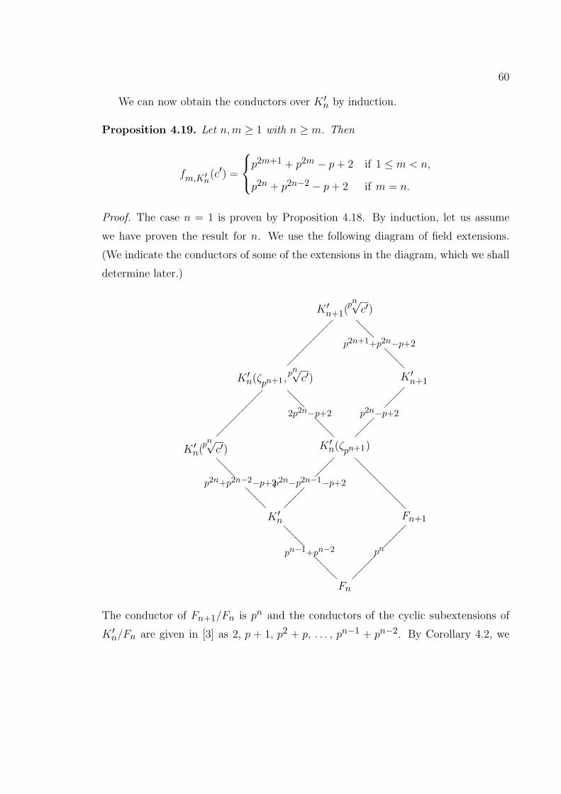
60

We can now obtain the conductors over K ′n by induction.

Proposition 4.19. Let n,m ≥ 1 with n ≥ m. Then

fm,K′n(c′) =

p2m+1 + p2m − p+ 2 if 1 ≤ m < n,

p2n + p2n−2 − p+ 2 if m = n.

Proof. The case n = 1 is proven by Proposition 4.18. By induction, let us assume

we have proven the result for n. We use the following diagram of field extensions.

(We indicate the conductors of some of the extensions in the diagram, which we shall

determine later.)

K ′n+1(pn√c′)

K ′n(ζpn+1 ,pn√c′)

��������������

K ′n+1

p2n+1+p2n−p+2??????

??????

K ′n(pn√c′)

��������������

K ′n(ζpn+1)

2p2n−p+2??????

??????p2n−p+2

������

������

K ′n

p2n+p2n−2−p+2???????

??????p2n−p2n−1−p+2

�������

������

Fn+1

????????????????

Fn

pn−1+pn−2???????

???????pn

�������

�������

The conductor of Fn+1/Fn is pn and the conductors of the cyclic subextensions of

K ′n/Fn are given in [3] as 2, p + 1, p2 + p, . . . , pn−1 + pn−2. By Corollary 4.2, we

61

have that the conductor of K ′n(ζpn+1)/K ′n is equal

2 + p(p− 1) + p2(p2 − 1) + · · ·+ pn−1(pn−1 − pn−3) + pn(pn − pn−1 − pn−2)

= p2n − p2n−1 − p+ 2.

By induction, we have that the conductors for K ′n(pn√c′)/K ′n are as in the state-

ment of the proposition. All but the largest of these is greater than p2n−p2n−1−p+2

Therefore, by Corollary 4.2, the conductors for K ′n(ζpn+1 ,pn√c′)/K ′n(ζpn+1) are the

same as those for K ′n(pn√c′)/K ′n except for the largest, which is

p2n − p2n−1 − p+ 2 + p(p2n−1 + p2n−2) = 2p2n − p+ 2.

To find the conductor of K ′n+1/K′n(ζpn+1), we need only convert the upper num-

bering of K ′n+1/Fn+1 to the lower numbering and find the largest jump in the filtra-

tion (plus one). This yields

2 + p(p− 1) + p2(p2 − 1) + · · ·+ pn(pn − pn−2) = p2n − p+ 2.

We next apply Corollary 4.2 again to find the conductors for K ′n+1(pn√c′)/K ′n+1.

Again, this changes only the final conductor, which becomes

p2n − p+ 2 + p(2p2n − p+ 2− (p2n − p+ 2)) = p2n+1 + p2n − p+ 2.

Thus we have determined the conductors fm,K′n+1(c′) for m ≤ n, and they match

those in the statement of the proposition.

Finally, noting that the ramification index of K ′n+1 is p2n+1(p − 1) and that

p2n+1 + p2n − p+ 2 > p2n+1 + 1, we conclude by Lemma 4.3 that

fn+1,K′n+1(c′) = p2n+2 + p2n − p+ 2,

which finishes the induction.

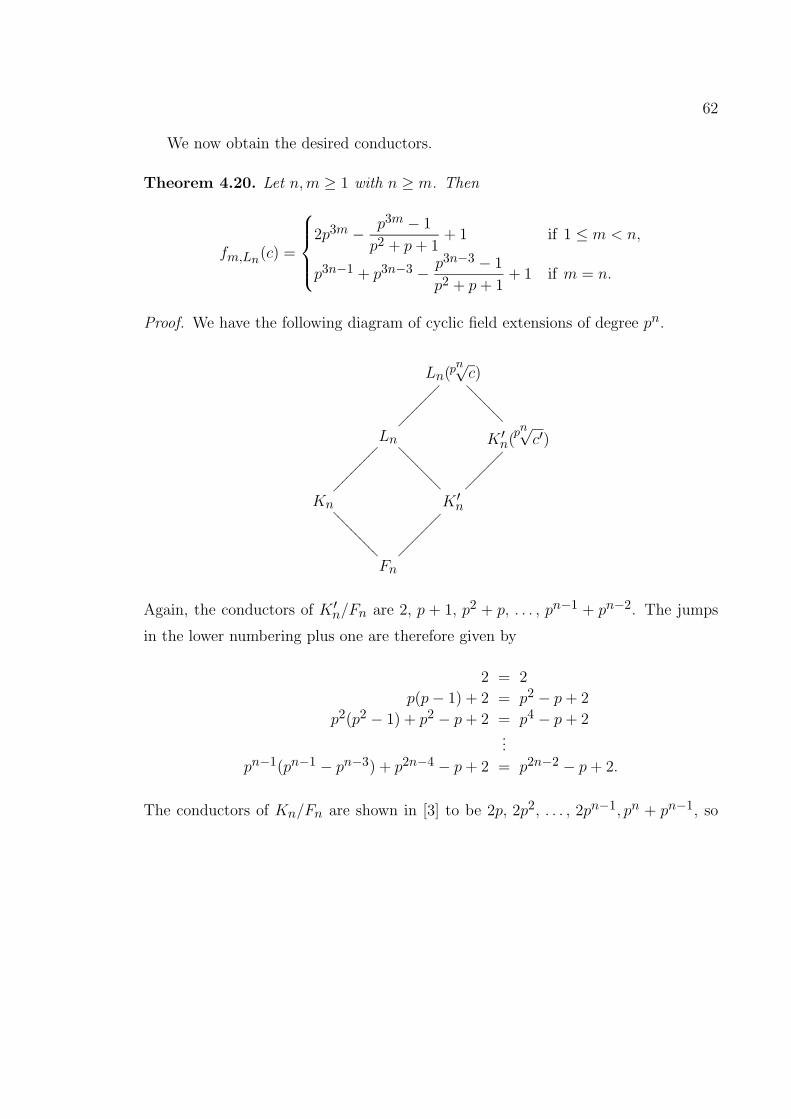
62

We now obtain the desired conductors.

Theorem 4.20. Let n,m ≥ 1 with n ≥ m. Then

fm,Ln(c) =

2p3m − p3m − 1

p2 + p+ 1+ 1 if 1 ≤ m < n,

p3n−1 + p3n−3 − p3n−3 − 1

p2 + p+ 1+ 1 if m = n.

Proof. We have the following diagram of cyclic field extensions of degree pn.

Ln(pn√c)

Ln

���������

K ′n(pn√c′)

????????

Kn

����������K ′n

?????????

��������

Fn

??????????

���������

Again, the conductors of K ′n/Fn are 2, p + 1, p2 + p, . . . , pn−1 + pn−2. The jumps

in the lower numbering plus one are therefore given by

2 = 2

p(p− 1) + 2 = p2 − p+ 2

p2(p2 − 1) + p2 − p+ 2 = p4 − p+ 2...

pn−1(pn−1 − pn−3) + p2n−4 − p+ 2 = p2n−2 − p+ 2.

The conductors of Kn/Fn are shown in [3] to be 2p, 2p2, . . . , 2pn−1, pn + pn−1, so

63

we have by Corollary 4.2 that the conductors of Ln/K′n are

p2(p− 1) + p2 − p+ 2 = p3 − p+ 2

p3(p2 − p) + p4 − p+ 2 = p5 − p+ 2...

pn(pn−1 − pn−2) + p2n−2 − p+ 2 = p2n−1 − p+ 2

pn(pn − pn−2) + p2n−2 − p+ 2 = p2n − p+ 2.

The conductors of K ′n(pn√c′)/K ′n are given by Proposition 4.19. Furthermore, we

have that the jumps in the filtration of K ′n/Fn in the lower numbering (plus one) are

given by

p3 − p+ 2 = p3 − p+ 2

p(p5 − p3) + p3 − p+ 2 = p6 − p6 − 1

p2 + p+ 1+ 1

...

pn−2(p2n−1 − p2n−3) + p3n−6 − p3n−6 − 1

p2 + p+ 1+ 1 = p3n−3 − p3n−3 − 1

p2 + p+ 1+ 1

pn−1(p2n − p2n−1) + p3n−3 − p3n−3 − 1

p2 + p+ 1+ 1 = p3n−1 − p3n − 1

p2 + p+ 1+ 1.

Finally, we apply Corollary 4.2 to obtain the conductors of Ln(pn√c)/Ln. We obtain

the following, as desired:

p(p2) + p3 − p+ 2 = 2p3 − p+ 2

p2(p4) + p6 − p6 − 1

p2 + p+ 1+ 1 = 2p6 − p6 − 1

p2 + p+ 1+ 1

...

pn−1(p2n−2) + p3n−3 − p3n−3 − 1

p2 + p+ 1+ 1 = 2p3n−3 − p3n−3 − 1

p2 + p+ 1+ 1

pn(p2n−2) + p3n−1 − p3n − 1

p2 + p+ 1+ 1 = p3n−1 + p3n−3 − p3n−3 − 1

p2 + p+ 1+ 1.

Remark. From the conductors of the various subextensions of L(pn√c)/Qp, one can di-

64

rectly compute the discriminant of entire extension. This could lead to a computation

of the discriminant for the corresponding extension of Q. With slightly more work,

one can compute the ramification groups of the entire extension over Qp. This would

provide an interesting example of the ramification groups of a three-step solvable ex-

tension: in particular, one could learn something about the jumps in the filtration in

the upper numbering of such an extension.

REFERENCES

[1] Brauer, Richard, “Uber die Konstruktion der Schiefkorper, die von endlichemRang in bezug auf ein gegebenes Zentrum sind,” J. Reine Angew. Math. 168(1932), no. 1, 44–64.

[2] Brattstrom, Gudrun, “On p-groups as Galois groups,” Math. Scand. 65 (1989),165–174.

[3] Coleman, R. F., McCallum, W., “Stable reduction of Fermat curves and Jacobisum Hecke characters,” J. Reine Angew. Math. 385 (1988), 41–101.

[4] Damey, P., Martinet, J., “Plongement d’une extension quadratique dans uneextension quaternionienne,” J. Reine Angew. Math. 262/263 (1973), 323-338.

[5] Damey, P., Payan, J.-J., “Existence et construction des extensions Galoisenneset non-abeliennes de degre 8 d’un corps de characteristique differente de 2,” J.Reine Angew. Math. 244 (1970), 37-54.

[6] Dedekind, Richard, “Konstruktion von Quaternionkorpern, Gesammelte mathe-matische Werke,” Band 2 (1931), Viewig, Braunschweig, 376–384.

[7] Gillard, Roland, “Plongement d’une extension d’ordre p ou p2 dans une surexten-sion non abelienne d’ordre p3,” J. Reine Angew. Math. 268/269 (1974), 418–426.

[8] Greither, Cornelius, “On Chinburg’s second conjecture for abelian fields,” J.Reine Angew. Math. 479 (1996), 1–37.

[9] Gross, Benedict, “Modular Forms (mod p) and Galois representations,” Internat.Math. Res. Notices 16 (1998), 865–875.

[10] Gross, Benedict, “Algebraic Modular Forms,” Israel J. Math., to appear.

[11] Ishkhanov, V. V., Lur’e, B. B., Faddeev, D. D., “The Embedding Problem inGalois Theory,” Translations of Mathematical Monographs 165, Amer. Math.Soc., 1997.

[12] Koch, Helmut, “Algebraic Number Theory,” Springer-Verlag, 1997.

[13] Lang, Serge, “Cyclotomic Fields I and II (Combined Second Edition),” Springer-Verlag, 1990.

[14] Serre, Jean-Pierre, “Galois Cohomology,” Springer-Verlag, 1997.

65

66

[15] Serre, Jean-Pierre, “Local Fields,” Springer-Verlag, 1979.

[16] Serre, Jean-Pierre, “Sur les representations modulaires de degre 2 de Gal(Q/Q),”Duke Math. J. 54, no. 1 (1987), 179–230.

[17] Massy, Richard, “Construction de p-extensions galoisennes d’un corps de car-acteristique differente de p,” J. Algebra 109 (1987), 508–535.

[18] Massy, Richard, “Formules de construction de p-extensions galoisennes,” C.R.Acad. Sc. Paris Ser. I Math. 303 (1986), no. 13, 591–595.

[19] Massy, R., Nguyen-Quang-Do, T., “Plongement d’une extension de degre p2

dans une surextension non abelienne de degre p3: etude locale-globale,” J. ReineAngew. Math. 291 (1977), 149–161.

[20] Sharifi, Romyar, “On Norm Residue Symbols and Conductors,” submitted forpublication. UIUC Algebraic Number Theory Preprint Archives, no. 149.

[21] Swallow, John R., “Central p-extensions of Galois Groups,” J. Algebra 186(1996), 277–298.

[22] Warfield, Robert B., Jr., “Nilpotent Groups,” Lecture Notes in Mathematics513, Springer-Verlag, 1976.

[23] Witt, Ernst, “Konstruktion von galoisschen Korpern der Charakteristik p zuvorgegebener Gruppe der Ordnung pf ,” J. Reine Angew. Math. 174 (1936),237–45.