The use of a body-wide automatic anatomy

recognition system in image analysis of

kidneys

S e y e d m e h r d a d M o h a m m a d i a n r a s a n a n i

ii

Master of Science Thesis in Medical Engineering

Stockholm 2013

This master thesis project was performed at Medical Image Processing Group

Department of Radiology

University of Pennsylvania

Under the supervision of Jayaram K. Udupa

The use of a body-wide automatic anatomy recognition system in

image analysis of kidneys

Seyedmehrdad Mohammadianrasanani

iii

Master of Science Thesis in Medical Engineering

Advanced level (second cycle), 30 credits

Supervisor at KTH: Hamed Hamid muhammed

Examiner:Manan Mridha

School of Technology and Health

TRITA-STH. EX 2013:119

Royal Institute of Technology

KTH STH

SE-141 86 Flemingsberg, Sweden

http://www.kth.se/sth

Summary

English:

In this thesis developed at MIPG, Upenn, we adapted, tested, and evaluated

methods and algorithms for body-wide fuzzy modeling and automatic anatomy

recognition (AAR) developed within MIPG in image analysis of kidneys. We built

a family of body-wide fuzzy models, at a desired resolution of the population

variables (gender, age), completed with anatomic, and organ geographic

information. The implemented AAR system will then automatically recognize and

delineate the anatomy in the given patient image(s) during clinical image

interpretation. My training also included gaining proficiency in large software

systems called 3DVIEWNIX and CAVASS which had an incorporation of all these

developments.

iv

Contents

1. Introduction

1.1. Basic concept of quantitative medical Imaging 1

1.2. Motivation 1

1.3. Hypothesis 2

1.4. Purposes and research topic 3

1.5. Literature review 3

1.6. The MIPG perspective and 3DVIEWNIX 5

2. Automatic Anatomy Recognition methodology 6

2.1. What is segmentation 7

2.2. Fuzzy modeling 8

2.3. Recognition 10

2.4. Anatomic definition for thoracic and abdominal objects 11

3. Adaptation of AAR to kidney segmentation 29

3.1. About kidney 29

3.2. Automatic recognition strategies 30

3.3. Image data 32

3.4. Experiments 33

3.5. Results and discussions 36

4. Conclusions 42

5. Acknowledgement 43

6. Reference 44

1. Introduction

1.1. Basic concept of quantitative medical Imaging

In this day and age, practice of Radiology is mostly qualitative. The physicians visualize the

images to make a clinical decision at individual patient level. Also, the accuracy of disease

recognition and reporting have been done by using biomarkers, and gathering volumes of image

information which could be time consuming and not very cost effective.

Quantification is a different approach to assess the normal values of anatomical sections of

different parts of the human body. As an analogy, blood sample analysis represents different

numbers that in turn indicates various parameters in the blood ranging from normal to abnormal.

Obviously, the number out of range can be detected as an abnormality (1).

1.2. Motivation: Why Quantitative Radiology (QR)?

The main motivation of this thesis is to study the applications of Quantitative Radiology (QR)

in clinical practice. Quantification has been investigated in clinical research, however only

descriptive and qualitative radiology is used for the patients in the hospitals. Through my thesis I

would like to prove that QR can be implemented in clinical practice as it can help improve early

diagnosis, standardize object (also referred to as organs) management, improve understanding of

normal disease processes, report and discover new biomarkers and to handle large volumes of

image data effectively.

This project helps visualizing more extensive knowledge in image processing, object

identification and delineation as it can have some clear cut advantages in routine clinical practice

for physicians and for the health care system. If QR can be adapted to clinical practice, it can

improve the diagnostic values which are determined by sensitivity, specificity and accuracy.

Why Automatic Anatomy Recognition (AAR)?

AAR is computerized automatic anatomy recognition during radiological image reading.

In order to achieve Quantitative Radiology we need body-wide Automatic anatomy recognition

(AAR) to make it more objective, improve specificity and sensitivity for disease detection.

Automatic recognition of the human inner organs from medical imaging data can make the

quantitative radiology feasible. Automatic anatomy detection which is based on fuzzy object

models (2-7) can provide the appropriate mathematical tools for creating fuzzy models which

1

2

can make it possible to extract the 3D models of organs from medical imaging data. Fuzzy and

probability principles start off with different axioms and use different mathematical constructs

and lead to different algorithms in images. Our motivation for using fuzzy objects modeling

principle is to find natural and getting object information extraction from images as realistically

as possible. In this thesis the focus was to see whether we can automatically recognize the kidney

and delineate the anatomy of the kidney, then the quantification is easy to take. We are using

AAR methodology to automatically detect kidney and study the kidneys.

Why kidney?

In clinical radiology practice, the interpretation of CT, MRI and PET images is typically

descriptive, qualitative or semi-quantitative at best. Although some approaches may be useful to

describe gross abnormalities that are present, they are often unable to detect early disease states

that may be present in tissues of the body, and are frequently unable to sufficiently characterize

disease conditions with high specificity. As such, quantitative assessments are required in order

to improve diagnostic assessment of imaging datasets obtained in the clinical setting.

The kidneys may be affected by various disease conditions, including benign focal lesions such

as cysts, oncocytomas, angiomyolipomas; malignant lesions such as renal cell carcinoma,

lymphoma, or metastases; infection (i.e., acute pyelonephritis); vascular disease such as by

vasculitis and infarction; and medical renal disease such as in relation to diabetes mellitus,

hypertension, glomerular disease, drug-induced nephropathy, amongst others. In the present

study, we are interested in applying quantitative assessment to abdominal MRI examinations in

order to better characterize focal lesions that occur in the kidney. The main reasons to perform

quantitative assessment in this clinical situation are to better characterize focal renal lesions as

benign or malignant, and to improve the ability to determine the histological type of focal renal

malignancy when present in order to optimize pretreatment planning and to prognosticate patient

outcome.

1.3. Hypothesis:

From the existing body-wide AAR system, we can quickly adapt to specific applications in

different body regions. Particularly in this project we are focusing on kidney and our claim is

that the AAR system can be adapted to recognize and segment the kidneys from datasets in

abdominal region. You do not have to start from the scratch to see how to segment the kidneys.

Therefore this thesis can lead to a better approach for kidney segmentation.

Specific hypothesis:

3

(1) One of the inputs of the model used for the AAR’s fuzzy model training is the hierarchical

relationship of organs that are distinguishable for the model. This hierarchical graph plays an

important role in the model and helps the recognition results to improve significantly. It is

claimed that a more detailed anatomical hierarchy improves the position error between the

predicted binary image produced by the AAR algorithm and the manually obtained one. This

hypothesis is tested for the data set comprised of CT images of abdomen with the kidney as a

target organ. It is claimed that the results are improved by adding an extra node (display children

of top most parent in views) to the anatomical hierarchy. This extra node could be a combination

of the target organ with some other organs. In this case both kidneys form a single node in the

hierarchy as parent node for each one of them which are the target organs. When we have

bilateral organs which means they are on both sides of the body having a hierarchy where two

are combined in one object and then subsequently separated to the individual objects will give a

better result. Results show a significant improvement although its cost in computation

consuming time is negligible.

(2) Different hierarchies may not give the same result for recognition.

(3) When you have an AAR system, it can be adapted to different modalities like MRI very

quickly.

1.4. Purposes and research topic:

Overall aim of this thesis is to adapt AAR methodology to the specific organ segmentation

problem which is our broad aim, which can be subdivided in several components: (A1) gathering

the training CT datasets for the different body regions – thorax (on computed tomography (CT)),

abdomen (on CT and magnetic resonance imaging (MRI)), (A2) gathering MRI datasets for

kidneys in abdominal region (A3) generate fuzzy model for these body regions especially for

abdomen because kidneys are located in the abdominal region (A4) investigating different

hierarchies to find out which hierarchies are most effective for the kidneys.

1.5. Literature review:

Several investigations (8-15) in kidney segmentation using both semi- automatic (9, 11, 12, 13)

and fully automatic methods (8, 10, 14, 15) have been carried on CT and MRI images. Despite

the important role of segmentation in medical imaging, difficulties are encountered due to the

associated variations in image quality. For example, certain conventional methods as

thresholding and region growing approaches (16) are often corrupted by noise, which can cause

difficulties in applying these methods. Among these methods, for the semi- automatic kidney

segmentation, they use optimal surface search with graph construction (11), segmentation of

kidney from high-resolution multi-detector tomography images that uses a graph cuts technique

4

(13). In the fully automatic methods, a constrained morphological 3D h-maxima transform

approach (8), graph cuts framework for kidney segmentation with prior shape constraints (14),

fully renal cortex segmentation on CT data sets using leave-one-out strategy (15).

Different approaches in the model processing part

Using the models including the prior information about shape and location of organs has been

considered in order to constrain the variations in the whole model processing (17, 18). Different

approaches have been reported in the whole model processing such as statistical theoretical

framework, statistical shape modeling (19), statistical atlases (20), and not taking a fuzzy

approach, except (2,3), both in the brain only. The novelty in our method is determined in the

following considerations: (A) focusing on a particular organ system in image analysis, which are

the kidneys. (B) Using fuzzy object models (2-7), which can provide the appropriate

mathematical tools to extract three-dimensional models of organs from medical imaging datasets.

Fuzzy set concepts have been used greatly, fuzzy modeling approaches allow brining anatomic

information in an all-digital form into graph theoretic frameworks designed for object

recognition. (C) Modeling a more detailed anatomical hierarchy, which plays an important role

in the model leading ultimately to the production of an effective AAR system. (D) Organizing

kidneys, left kidney, and right kidney in a hierarchy, encoding kidneys relationship information

in to the hierarchy. And (E) using optimal threshold-based recognition method, which is

powerful concept with consequence in the kidneys recognition and delineation.

There are several steps involved in the Automatic Anatomy Recognition of the kidneys (AAR-

QR) project; 1- collecting whole body imaging data from normal subjects 2- building and

assessing fuzzy models 3- applying these fuzzy models in order to recognize and delineate

anatomy in a certain diseased subject. (2-7)

In this project, we evaluated different organs to create several object’s models in this age group.

Modeling processes had to be done with care, because it is problematic that many of these organs

have no proper definition of the boundary in a mathematical sense. For example, we all

understand what kidney means but when it comes to identifying kidneys’ boundary on CT or

MRI images as a specified object becomes really challenging, even for some well-defined

objects like liver. The problem is not only with kidney, but all open objects in the thorax and

abdomen. Therefore, the first thing is to define the exact thoracic and abdomen regions, where it

starts and where it ends. Then, work through all these areas, and come up with an overall

definition that is comprehensible by physicians and radiologists.

In organ like kidney, there are vessels and lymphatic system which can potentially cause some

issues while defining the boundary. Therefore, in order to avoid this, an expert has to define the

boundary of the object and come up with some operation definition that could be applied to all

the subjects in a very consistent manner.

5

Thus, it is very crucial to follow these steps to build a fundamental method to automatically

process the modeling, recognition and delineating the anatomy in patient’s images.

The modeling is based on hierarchy, which divides the body into separate parts like thorax and

abdomen. It has been clear that there is no way to define the best hierarchal manner in the whole

body, so certain organ hierarchy leads to obtain better results. Regarding this point the

anatomical and computational organizations are not necessarily the same.

For building this model, there are specialized tools that have already been developed for both

thorax and abdomen called the 3DVIEWNIX.

Regarding the object definition and variation, there are also variations in the whole model

processing itself. Bigger people may not necessarily have larger organs. The anatomy of some

organs is independent of the size of the person. Some of them are symmetrical. For example, left

and right kidney is considered as pair of organs with a fixed relationship, correlating among

object size. They often have a high correlation in size. It means that, if one gets bigger then the

other also becomes bigger, however these do not apply to all organs. Some organs even show no

correlation or negative correlation, in geographic terms we can consider the relationship of the

organs.

The scene is an image, which is the main type of data. It refers to multidimensional images like 2

dimensional (2D), 3D, 4D, and all the data that are handled in 3D. Fuzzy boundary is represented

in different ways. For example, there is some source of the object in the image where it is not

possible to make a hard decision, for doing segmentation in unclear objects; we have uncertainty,

which typically is the region of boundary with pixel values. Fuzzy modeling approach allows

capturing information about uncertainties at the patient level (e.g., partial volume effect) and

organizing this information within the model.

1.6. MIPG perspective and 3DVIEWNIX

3DVIEWNIX has been developed and maintained by the Medical Image Processing Group. It

has been employed by hundreds of sites. It is a powerful instrument which provides a variety of

sophisticated approaches to manipulate, visualize and quantify structure information captured in

multimodality image data. The operators will be able to employ a various processing paths

through 3DVIEWNIX to achieve their study aims. (21)

3DVIEWNIX is based on the UNIX operating system, X-Windows, and the C programming

language. The basic philosophy of 3DVIEWNIX is that we have focused in medical images

which are applicable in 2 dimensional (2D), 3D and 4D, in fact it is set up for n dimensional

images. Some operations can do for 2 and 3 dimensional and some of them for 4D. You can

consider images with the same body region but using deferent modality like CT and MRI since

they give different types of information.

You need to define the object in images, for instance preprocessing can do this with defining the

object, segmenting it explicitly or improving the object information by enhancing object

information in different ways.

6

2. Automatic Anatomy Recognition methodology

The AAR methodology is graphically summarized in Figure 1. The body is separated into M

body regions B1… BM. Models are constructed for each specific body region and each population

group G. Three main blocks in Figure 1 correspond to model building, object recognition, and

object delineation. A fuzzy model FM(Oℓ) is constructed separately for each object Oℓ in B. ℓ=1,

…, L, and these models are integrated into a hierarchy selected for each specific body region B.

The output of the first step is a fuzzy anatomic model FAM(B) of the body region B. This model

is employed to recognize objects in a given case image I of the specific body region B belonging

to the specific population group G in the second step. The hierarchical relationship of organs is

tracked in this process. The output of this step is the set of transformed fuzzy models FMT(Oℓ)

corresponding to the state when the objects are recognized in I . These adapted models and the

image I form the input to the third step of object delineation which also tracks the hierarchical

relationship of organs. Finally the delineated objects are output as Images (2-7)(cf. fig. 1).

7

There are three components from our perspective. Describing concepts, methods and algorithms,

and also in the given image how one can recognize and delineate automatically. Once you

recognize and delineate the anatomy, quantification is easy to make.

2.1 What is segmentation?

Segmentation consists of assigning a label to every pixel in an image such that pixels with the

same label share the same characteristics, like being part of the same organ. In fact, outlining

images can be done either in hard or fuzzy way. It is very difficult to do fuzzy way for human; it

Recognize other objects as per hierarchy

hhihierarchy

Gather image database for & G

Delineate O1, …, OL in images

Construct fuzzy model of for G

Model Building

Object Recognition

Recognize root object

Object Delineation

FAM()

FMT(Ol), l = 1, …, L

Figure.1 a schematic representation of the AAR methodology

8

should be done only in the hard way. Segmentation consists of two tasks, recognition and

delineation. Recognition is the high level task and is done with determining the object

whereabouts in the scene, usually humans are more efficient than the computers to get this high

level knowledge, but in delineation which is to determine the objects spatial extent and

composition in the scene which is a low level task and very detailed quantitative task, usually

computers do better than humans.

There is a large amount of publications about segmentation since image processing started. The

method can be classified into three groups:

First, PI (purely image based) approach (6): Collecting the whole available information in an

image and determining the best way of performing recognition and delineation. In most methods,

recognition is done manually which actually specifies something and delineating is done

automatically which mostly relies on available information in the given image only. (22-28)

The second method is shape model based (SM) approach (29-32): employing models to code

object family shape information, recognition is based on model and it can be manual or the

combination of both, the whole idea is to bring the model to perform recognition and delineation.

The third method is Hybrid approach: which is the combination of PI and SM approaches, in this

method recognition is based on the model and can be done automatically. (33-36)

2.2. Fuzzy modeling

Notation: We will use the following notation throughout this thesis. G: the population group

under consideration. B: the body region of focus. O1...OL: L objects (also referred to as organs)

of B (such as kidney, liver, etc. for B= Abdomen) considered in B for AAR. We are focusing on

fuzzy model and fuzzy model steps in a set of images and different subjects (N) because we are

building the model for the normal subjects. I1 ……….IN: Images for body region (B) and

subjects all from a particular population group G. In,ℓ: the binary image representing the

delineation of object Oℓ in the image I. FAM(B): Fuzzy anatomic model of the whole object

assembly in the body region B with respect to its hierarchy since each specific body region has

its own hierarchy. FMT(Oℓ): Transformed FM(Oℓ) corresponding to the state when Oℓ is

recognized in a given patient image I.

Gathering image database for B and G

Gathering body wide group wise image data for normal subjects, our essential ponder is that

model should reflect what is normal based on our experience working in different applications

and modalities. Normality is easier to model and the images were of high quality and visually

appeared radiologically normal for the body region, that is why we are focusing on normal

datasets. Our modeling schema is such that the population variables can be defined at higher

“resolution” in the future and the model can then be updated when more data are added. For the

9

thoracic and abdominal body regions, a board certified radiologist selected all image data (CT

and MRI) from our health system patient image database.

Delineating objects of B in the Images

There are two parts to this task – forming an effective definition of the specific body region B

and the organs in B in terms of their precise anatomic extent, and then delineating the objects

following the effective definition.

Delineation of objects: We can use some interactive tools, some manual tools and also some

automatic tools. Through a combination of methods including live wire, iterative live wire (40)

thresholding, and manual painting, tracing and modification. For instance, in the abdomen, to

delineate kidney as an object by using the iterative live wire method. (Iterative live wire is a

version of live wire in which once the object is segmented in one slice, the user commands next

slice, the live wire then runs automatically in the next slice, and the process is continued until

automatic outlining fails when the user resort to iterative live wire again, and so on). In MRI

images, the same approach works if background non-uniformity correction and intensity

standardization (41) are applied first to the images.

All segmentation results of the objects were examined for accuracy by several checks –

generating 3D surface renditions of objects form each subjects in different objects combination

as well as a slice-by-slice confirmation of the delineations overlaid on the gray images for all

images.

Constructing fuzzy object models

The Fuzzy Anatomy Model FAM (B) of body region B for G is defined to be a quintuple: (2-7)

FAM (B) = (H, M, ρ, ʎ, ƞ). [1]

Briefly, the overall definition of the five elements of FAM(B) is as follows. The first item is

hierarchy (H) of the objects in the specific body region B. M is a set of fuzzy models; one fuzzy

model associated with each object in B. ρ defines the parent-to-offspring relationship in

hierarchy H over the specific population group G. ʎ expresses a set of scale factor ranges

indicating the size variation of each object Oℓ over the population group G. ƞ represents a set of

measurements pertaining to the organs assembly in B (ƞ, could be used to measure the volume of

the objects). A detailed explanation of these elements is presented below.

Hierarchy: H is expressed as a tree, of the objects in B. The idea is that, the whole body itself has

middle tree, a root of the tree and different body region are different aspects and within these

concepts each body region has its own hierarchy. For example, for thorax the root is the skin

10

boundary and everything else means other organs within the body region, there are some other

hierarchy that can be used for the specific task of segmenting one or two specific objects like the

kidneys.

M = {FM(Oℓ): 1 ≤ ℓ ≤ L} is a set of fuzzy models, one model per object. We are given the

segmented images then they are outlined for object then fuzzy model expresses the fuzzy set that

is the value of the voxel and indicates membership, so fuzziness that comes from the fact that

these are for instance fifty different livers or lungs or kidneys, they are identical in size, position,

orientation and shape, the idea of creating the fuzzy is to average them, so overlapped areas,

maximize membership. (2-7)

ρ describes the parent-to-offspring relationship in H over G: ρ = {ρℓ,k : Oℓ is a parent of Ok, 1 ≤ ℓ,

k ≤ L}. It also encodes whole body to body region relationships. If you take the center of Oℓ and

center of Ok there are certain relationship geometrically.

ʎ is a set of scale ranges ʎ = {ʎℓ=[ʎb

ℓ ,ʎh

ℓ] : 1 ≤ ℓ ≤ L} indicating the size variation of each object

Oℓ over G. The size of the object can be expressed in a number. We can resize all of them to the

same size. If you take one number, one possibility is the volume and scale factor. In scale factor,

if you come up with one idea in the size of the object, you find the mean size and then scale

everyone to the mean size so that it gives you the scale factor for every object. Also for every

subject, so that scale factor has a variation over the population that can be different for every

object. This information is made use of recognizing Oℓ in a given image to limit the search space

for its pose. ƞ represents a set of measurements pertaining to the objects in B. For details, see (2-

7).

2.3 Recognition

Recognition is a high-level process of determining the whereabouts of an object in the image.

The second step is recognition. The goal of recognition is to determine where objects Oℓ are in

a given test image I, to determine the best pose (location, orientation, and scale factor) of

FM(Oℓ) in I, 1 ≤ ℓ ≤ L. We recognize the root object first in the hierarchy H. There is an initial

global recognition step whose goal is an initial pose of FAM(B) in I in close to the known true

objects in the binary images. This process is adjusted consequently hierarchically by using the

parent-to-offspring relationship ρℓ,k. The children Ok are recognized by knowledge of the pose of

their already recognized parent Oℓ .Root object should be used in the model for the given image.

The best status of the position and orientation are known in the recognition. Then we can follow

the hierarchy and parent’s objects relationship and the scale information. During the offspring

object recognition, object’s root recognition is different with the recognition of the objects in the

hierarchy; in fact we have several methods to do this.

11

There are many techniques for recognition depending on the types of objects such as: b-scale

method, Fisher linear discriminate, optimum threshold and hierarchical registration. (37, 38, 39)

For all of them we search the optimal method and also the optimal position for each case,

depending on definition of the automation criteria. We have tested three methods and optimum

threshold is the best one. If you do the recognition then you know that for every object in a given

image position, orientation and size should be considered, once you provide that information

then you need to do delineation.

2.4. Anatomic definition for thoracic and abdominal objects

We have conducted detailed analysis and review of the thoracic objects; there are numerous

disparities and inconsistencies found, in the segmentation of various thoracic objects. To correct

this issue and ensure consistency of the objects throughout all the subjects, we have refined the

anatomic boundaries and definition of various thoracic objects. The 13 objects in the thoracic

region are illustrated below in hierarchy (cf. fig. 2).

Figure.2 the 13 objects in the thoracic region are illustrated in hierarchy: tskin: thorax skin

boundary; tb: trachea and bronchi; lps: left pleural space; rps: right pleural space; pc:

pericardium; tsk: thoracic skeleton (previously bone); as: arterial system; vs: venous system; e:

esophagus; rs: respiratory system (lps+rps+tb); ims: internal mediastinum (pc+as+vs+e); tscrd:

spinal cord; stmch: stomach.

This expresses the outline of the important correction and refinement made to the objects.

The anatomic boundary of the thoracic region can be simply defined as the region starting from

the base of the lung, all the way up to the apices of the lungs. More precisely, the inferior

anatomic extent of the thoracic region, starts from 1 standard CT-axial slice below the first

12

appearance of the lung. Equals 5 mm below the first appearance of the lung, and the superior

anatomic extent is defined up to, 3 standard CT –axial slices, above the apices of the lung (equal

15 mm above the apex of the lung).One slice in our axial CT patient images corresponds to 5

mm. in all images the slices go up from the base of the lungs to their apex (cf. fig. 3).

Figure.3 the anatomic boundary of the thoracic region

Tskin –thorax skin

The skin is segmented following the anatomic boundaries of the thoracic region, as described

before. So, the inferior extent of segmentation for skin starts from one slice below the first

appearance of the lungs. And the superior extent is marked by 3 standard CT- axial slices above

the apices of the lungs. More precisely, the inferior extent anatomically bottom- most) of skin, is

marked by 1 standard CT –axial slice, below the first appearance of the lung, (equals 5 mm

below the first appearance of the lung) and the superior anatomic boundary for skin is all the way

up to three standard CT axial slices above the apices of the lungs (cf. fig. 4).

13

(a)

(b)

(c)

Figure.4 (a) the anatomic boundary of the tskin, (b) the axial CT slice with overlaid tskin

segment (c) 3D rendered tskin object.

RS –respiratory system

The respiratory system is an combined object of the individual objects namely, LPS –left

plural sac, RPS–right plural sac and TB –trachea bronchi (cf. fig. 5).

14

(a) (b)

Figure.5 (a) the axial CT slice with overlaid rs segment (b) 3D rendered rs object.

LPS – left plural sac

The inferior extent of the left plural sac is defined by the base of the lung, the first appearance

of the left plural sac, on the bottom- most slice, and the superior extent is defined by the apex of

the left lung (cf. fig. 6).

Figure.6 the axial CT slice with overlaid lps segment.

RPS –right plural sac

15

The inferior extent of the right plural sac is defined by the base of the lung, the first appearance

of the right plural sac, on the bottom-most slice, and the superior extent is defined by the apex of

the right lung (cf. fig. 7).

(a) (b)

Figure.7 (a) the axial CT slice with overlaid rps segment (b) 3D rendered rps object.

Trachea and bronchi –tb

The superior/top anatomic boundary for segmentation of tb would be marked by the last axial

slice, in the upper thoracic region, where the trachea is visible. And the tb is segmented all the

way down, towards the inferior boundary, including the branching of trachea into the left and

right bronchi. The main structure of left and right bronchioles is included, whereas the secondary

branches and bronchioles are excluded. From a simple visual perspective, the ‘general upside-

down Y’ structure was included with all the additional branches cut off/excluded.

The superior boundary is marked by the superior anatomic delimiting plane for tb, i.e. until

trachea is visible in the upper thoracic region (cf. fig. 8).

16

(c) (d)

Figure.8 (c) the axial CT slice with overlaid tb segment (d) 3D rendered tb object.

Tsk –bone

The bone is segmented all the way through the body region, from the posterior to anterior

boundary of the skin (cf. fig. 9).

17

(e) (f)

Figure.9 (e) 3D rendered tsk object, (f) the axial CT slice with overlaid tsk segment

Ims –internal mediastina system

The ims is a combined object, which includes the following objects pc -pericardium, e –

esophagus, as –arterial system and vs –venous system (cf. fig. 10).

Figure.10 3D rendered ims object.

Pericardium –pc

18

In theory, pericardium is a double- walled sac containing the heart and the roots of the great

vessels (cf. fig. 11a). But, in the reality, the vessels that emerges out of the pericardium and are

seen more visibly as discrete structures and the enclosing sac is not always explicitly visible on

the axial CT slices. We have decided to consistently define the pericardium by tracing the actual

boundary- pericardial sac itself.

The top boundary or the extent to which the vessels are to be included and the anatomic point of

reference for the anterior- top boundary will be marked by the plane/axial slice where the

pulmonary trunk starts to branch out to the right/left pulmonary artery. (cf. fig. 11b).

(a) (b)

Figure.11 (a) the anatomical information of the pc object, (b) 3D rendered pc object

Esophagus –e

The segmentation of esophagus starts in the inferior/bottom section, from the first slice of the

thoracic region and all the way to the top superior/top section, until the plane/axial –slice where

the trachea is visibly seen. In other words, the superior/top anatomic boundary of the object tb is

also considered the superior delimiting point of reference or the upper cut-off point for

esophagus.

In anatomic terms, the anterior extent of esophagus is segmented from the very first bottom-

most slice of the thoracic region all the way through up until the superior/top anatomic boundary

of trachea –i.e., until trachea is visible. (cf. fig. 12).

19

(g) (h)

Figure.12 (g) the anatomical information of the e object, (h) 3D rendered e object.

Arterial system –as

The inferior anatomic boundary, for segmenting as, starts from the first slice of the thoracic

region (anatomically bottom- most), and the superior/top anatomic boundary is the anatomic

extent to which, the three arteries that arise from the aortic arch, are included into as. In abstract

terms, we include the aorta, ascending aorta, the aortic arch and the three arteries that rise from

above the aortic arch. In the superior extent of as, the brachiocephalic artery, left common

carotid artery and left subclavian artery should be included all the way until the plane/axial –slice

where any of them start to branch out. In other words, the axial-plane at which any of these three

arteries starts to branch out acts as our cut- off point for the superior section or boundary. The

inclusion of pulmonary trunk starts from the plane/axial –slice where the ascending aorta first

appears. In fact traversing from the inferior to superior section in while segmenting, the

appearance of ascending aorta acts as our anatomic point of reference to start tracing the

pulmonary trunk. (cf. fig. 13).

20

(a) (b)

Figure.13 (a) the anatomical information of the as object, (b) 3D rendered as object.

Venous system –vs

The inferior extent of segmentation of vs starts from first (anatomically bottom- most) slice,

where the azygos vein is visible. And the superior/top anatomic boundary or the cut-off would be

the plane/axial-slice where the secondary branches on the brachiocephalic veins start. vs segment

would include the azygos vein (the azygos branches and sub-branches are not included), superior

vena cava and right and left brachiocephalic vein, where one of the brachiocephalic veins is

separating into two or more branches. (cf. fig. 14).

21

Figure.14 3D rendered vs object

All the above defined objects, for n= 50 subjects, have been refined and corrected accordingly.

These revisions and refinements to the anatomic boundaries and definitions of the thoracic

objects would facilitate the accomplishment of more consistency thorough the objects, thereby

producing crisper models.

We have conducted analysis for most of the abdominal objects. To ensure consistency of the

objects throughout all the subjects, we have refined the anatomic boundaries and definitions of

various abdominal objects, which are outlined in this document (cf. fig. 15).

22

Figure.15 (a) the 11 objects in the abdominal region are illustrated in hierarchy. aia: aorta until

bifurcation to iliac arteries; asft: abdominal soft tissue (mscl + spln + rkd + lkd + aia + ivc); ask:

abdominal skeleton; askin: abdominal skin; ivc: inferior vena cava; lvr: liver; lkd: left kidney;

mscl: muscle; rkd: right kidney; spln: spleen; sat: subcutaneous adipose tissue.

Definition of abdominal region:

The inferior anatomic boundary of the abdominal region can be simply defined by the

plane/axial slice where the union of the right and left common iliac arteries is anatomically

represented by the top-most, axial slice that marks the top/superior aspect of the liver (cf. fig.

16).

23

Figure.16 the anatomic boundary of the abdomen region

Askin-abdominal skin

The skin is segmented following the anatomic boundaries of the abdominal region, as

described before. So, the inferior extent of segmentation for skin starts from the slice where the

common iliac arteries unite and form the aorta. And the superior extent is marked by the axial

slice, where the superior part/top of the liver is seen in the upper abdominal region (cf. fig. 17).

Figure.17 the anatomic boundary of the askin object

24

Abdominal skeleton –ask

The segmentation of ask is in below. (cf. fig. 18).

Figure.18 3D rendered ask object

Asft, this is a combined object obtained by including the individual objects namely, Muscle,

spleen, right kidney, left kidney, Aorta and iliac artery, inferior vena cava.

Lvr- liver

The superior anatomic boundary for the segmentation of liver, would lie on the plane/axial-

slice where the top- most part of liver appears. And the inferior anatomic boundary would be

defined by the plane/axial-slice, where the liver first starts to appear.

The portal and hepatic arteries and veins are included when approaching and entering into the

liver and extraneous extensions are excluded (cf. fig. 19).

25

(b) (c)

Figure.19 (b) the anatomical information of the lvr object, (c) 3D rendered lvr object

Sat, the subcutaneous adipose tissue (sat), refers to the layers of fat, right beneath the skin.

The sat is segmented using the following approaches:

To segment subcutaneous adipose tissues as an object, the skin outer boundary (as an object) is

first segmented by using the iterative live wire method (40). Subsequently, the interface between

the subcutaneous and visceral adipose compartments is delineated by using also the iterative live

wire method. Once these two object boundaries are delineated, the subcutaneous and visceral

components are delineated by using thresholding and morphological operations. (cf. fig. 20).

Figure.19 3D rendered sat object

26

Spl-spleen

The superior and inferior extent for the object, spleen, is defined by the extent of boundary of

the object itself. In other words, the spleen is segmented from and to where it actually starts and

ends on the axial slices.

The actual sac like, physical spleen structure cleanly segment from the start to end of the object,

the extraneous structures like the vessels which enter into and come out of the spleen, are

excluded (cf. fig. 21).

Figure.21 3D rendered spl object

Rkd- right kidney and lkd- left kidney

The superior and inferior anatomic boundary for both right and left kidneys is defined by the

superior and inferior boundaries of the individual objects itself. In other words, the right kidney

is segmented from the inferior boundary of the right kidney all the way up to the superior

boundary of the right kidney. The same applies to the left kidney as well.

Based on review, we have decided that the segmentation would follow and include the actual

bean shaped structure of the kidney. All the other external blood vessels (viz, renal arteries, renal

veins) are excluded (cf. fig. 22)

27

Figure.22 3D rendered lkd and rkd objects

Figure.23 the anatomical information of the

kidneys object

Aorta and iliac arteries

The superior and inferior boundaries of the aia are defined by the pre-defined boundary of the

abdominal region. Anatomically, aia includes the abdominal aorta, from the point of union of

common iliac arteries, all the way up to the aorta, delimited by the superior boundary of the

28

abdominal region. We include only the structure of aorta through this region and the

branches/sub- branches of arteries are not included (cf. fig. 24).

(e) (f)

Figure.24 (e) the anatomical information of the aorta and iliac arteries objects, (f) 3D rendered

aia object

IVC –inferior vena cava

Anatomically, ivc includes the inferior vena cava, from the point of union of iliac veins, all the

way up, until the delimitation by the superior boundary of the abdominal region. We only

include the actual structure ivc; the branches/sub- branches of veins, are not included (cf. fig.

25).

29

Figure.25 3D rendered ivc object

Muscle -mscl (cf. fig. 26).

Mscl is delineated by using thresholding and morphological operations as the same procedure for

sat.

Figure.26 3D rendered mscl object

30

3. Adaptation of AAR to kidney segmentation

3.1. About kidney

The kidneys are a pair of organs located in the back of the abdomen the size of each kidney is

about 4 or 5 inches long [length – about 12 cm breath- about 6 cm thickness], the average weight

of a normal, healthy adult kidney is approximately 120-140 grams. The kidney helps maintain a

constant environment within the body and also the kidney regulates water and electrolyte levels

within narrow limits and removes waste metabolic products and foreign toxin. The kidney

regulates Red blood cell concentration and maintains blood pressure in our body. They are

essential in the urinary system and serve the body as a natural filter of the blood.

There are different types of kidney diseases and also different types of kidney cancer exist like

renal cell carcinoma which is one of the most common cancers.

Figure.27 the anatomical information of kidney object

31

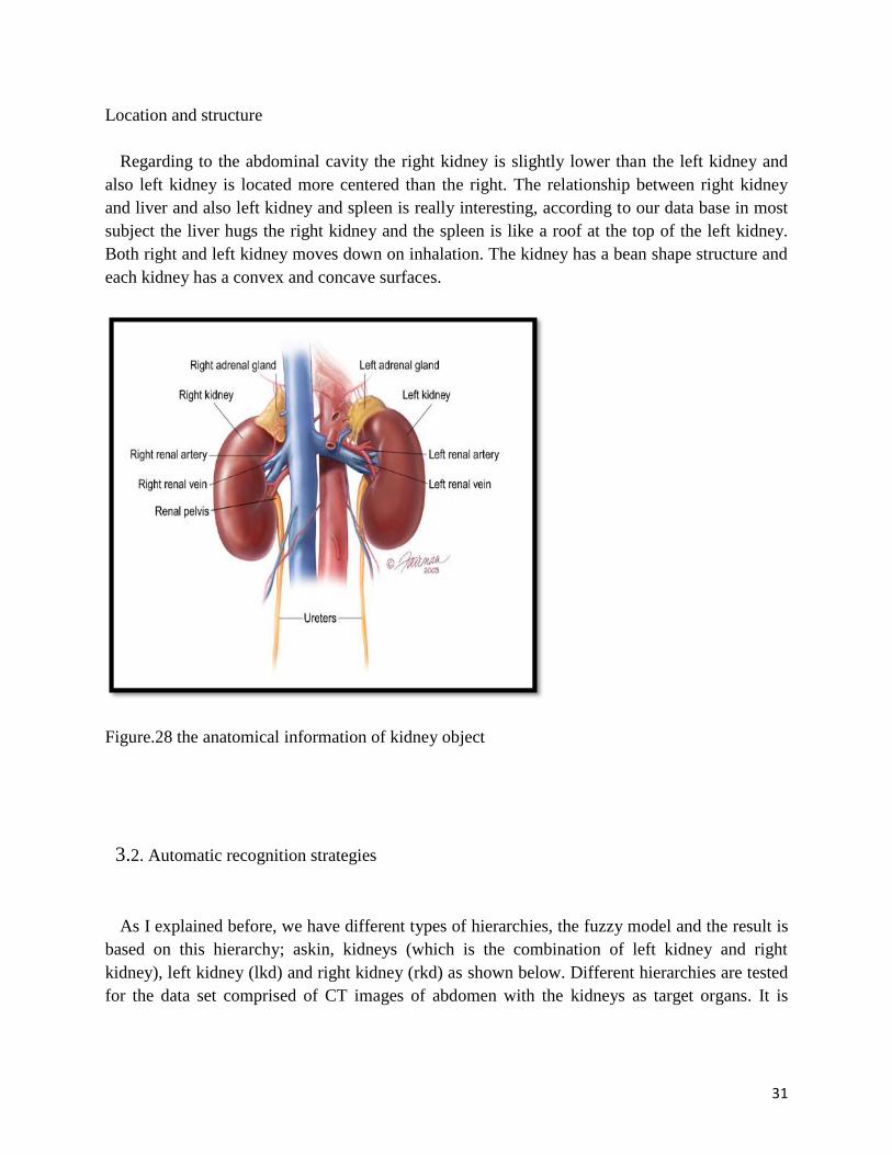
Location and structure

Regarding to the abdominal cavity the right kidney is slightly lower than the left kidney and

also left kidney is located more centered than the right. The relationship between right kidney

and liver and also left kidney and spleen is really interesting, according to our data base in most

subject the liver hugs the right kidney and the spleen is like a roof at the top of the left kidney.

Both right and left kidney moves down on inhalation. The kidney has a bean shape structure and

each kidney has a convex and concave surfaces.

Figure.28 the anatomical information of kidney object

3.2. Automatic recognition strategies

As I explained before, we have different types of hierarchies, the fuzzy model and the result is

based on this hierarchy; askin, kidneys (which is the combination of left kidney and right

kidney), left kidney (lkd) and right kidney (rkd) as shown below. Different hierarchies are tested

for the data set comprised of CT images of abdomen with the kidneys as target organs. It is

32

shown how the results are improved by adding an extra node to the anatomical hierarchy and

also different types of hierarchies may not give the same result for recognition (cf. fig. 29).

Figure.29 the 4 objects in the abdominal region are illustrated in hierarchy. Askin; kidneys

(which is the combination of left kidney and right kidney); left kidney (lkd) and right kidney

(rkd).

The recognition result is based on optimal thresholding which is an important concept.

Meaning that optimization is a vast branch of mathematics. The hierarchical order also is

followed in this method. Optimal thresholding method uses known (learned) fixed object

threshold interval and minimal false positive and false negative of the threshold image with

respect to FM(Oℓ) for best recognition. For MRI images for this approach to make sense, it is

essential to correct for background intensity non-uniformities arising from magnetic field

inhomogeneity first, followed by intensity standardization (40). So in this context the root object

is recognized first, for the hierarchy shown in Figure 28, the root object is the skin outer

boundary. There is a global approach, which does not involve searching for the best pose. We

call this the One-Shot Method which is used as initialization for a more refined optimal

thresholding method. (2-7)

One-Shot Method

33

We know approximately what the threshold for the root object O1 is (by applying a threshold to

I), and then from that approximate threshold you can roughly segment O1 to produce a binary

Image. The goal of the one-shot method is to find the mean relationship, estimated from the

training images, between the roughly segmented O1 and the true segmentation of O1. This

estimation can be specified by the geometric center from the set of 1-voxels of any binary image

and the eigenvectors derived from X via principle component analysis. Similar thresholding is

performed on each gray image In in the training datasets to acquire a rough segmentation of O1.

The mean, of such estimation over all training images is done at the model building stage of

AAR. The pose of all other objects are adjusted consequently hierarchically by using parent-to-

offspring relationship ρℓ,k.

Optimal thresholding method

This is a method to refine the result found from the one-shot method, starting from the initial

pose obtained by the one-shot method, a search is made within the pose space for an optimal

pose of the fuzzy model that yields the smallest sum of the volume of false positive and false

negative regions. It should be considered that the model itself is taken as the reference for

defining false positive and false negative regions. As the model is fuzzy so at every voxel there is

a membership, therefore when you find the threshold for given interval you get the binary image,

in this context the false positive and false negative correspond to the disagreement between the

membership of the fuzzy model and the thresholding result. The search space to find an optimal

pose is limited to a region around the initial pose. This region is determined from a knowledge of

ρℓ,k and its variation and the scale factor range ʎ.

Determining the optimal threshold interval at the model building stage

Suppose we already built fuzzy model and estimated ρ and ʎ. We run the recognition process

on the training datasets. Since we still do not know the optimal threshold but have the true

segmentations made by a person. The process is to test out recognition ability for each of a

number of threshold intervals and then select the threshold interval that yields the best match of

the model with known true segmentation for each object.

To summary, the optimal threshold method of recognition consists of three steps: (a) starts the

search process from the initial pose indicated by the one-shot method. (b) It uses the optimal

threshold values determined from the training datasets for each object. And (c) finds the best

pose for FM(Oℓ) in the given image I by optimally matching the model with thresholded image I.

3.3 Image data

34

CT datasets: We focused on males aged 50-60 years old with normal hospital data base in

thorax and abdomen. The images are acquired using breath-hold CT, they were contrast

enhanced, their size and their level of digitization was 0.9*0.9*5 mm, the slice basing (basis)

was 512*512*80 pixels/voxels. The number of subjects was 50.

For those regions in 50-60 subjects, we have used half of the data base for creating the model

and the other half for testing it.

MRI datasets: we focused on males and females aged 28-78 years old with various focal renal

pathologies (normal, cysts, angiomyolipomas, and renal cell carcinomas of different types) in

abdomen with the kidneys as target organs. They were T1-weigthed, axial post contrast

enhanced, delayed phase, their size and their level of digitization was 0.7*0.7*4-5mm, the slice

basing (basis) was 512*512*40-69 pixels/voxels. Manufacturer: GE medical systems,

manufacturer’s model name: GENESIS_SIGNA, magnetic field strength: 15000, spacing

between slices: 7. Repetition time TR: 1210.54 msec. Eco time TE: 183.55 msec. In the case of

MRI, the resulting images are processed, first to suppress background non-uniformities and

subsequently to standardize the image intensities (41). Standardization is done separately for

each MRI case. The number of subjects was 17.

3.4 Experiments

These are some examples of thorax and abdomen objects that we have used in the model

building FM(Oℓ). Since the volumes are fuzzy, they are volume rendered by using an appropriate

opacity function. The objects that we have considered look like a picture collection. It is

important to understand the relationship between the objects and the way the objects fit together

in terms of relationships and also core identifications.

It looks like they enfold each other; there is a lot of prior information about object’s specific

relationship for every subject consistently. For example, in the aorta and inferior vena cava and

the kidneys how the same angles in to the same cross, and also spleen and left kidney enfold

each other very nicely, and muscle and soft tissue. (cf. fig. 30).

35

Figure.30 renditions of objects used for modeling from two body regions (abdomen and thorax)

36

37

Figure.31 volume rendition of fuzzy model for abdomen and thorax in different combinations of

the objects

38

3.5 Results and discussions

Results for recognition are summarized in Figures 32-33 and Tables 1-4 for the kidneys as target

organs. The recognition accuracy is expressed in terms of position and size. Values 0 and 1 for

the two measures, respectively, indicate perfect recognition. The position error is expressed as

the distance between the geometric centers of the known true objects in the binary images and

the center of the adjusted fuzzy model FMT(Oℓ). The size error is expressed as a ratio of the

estimated size of the object at recognition and true size.

(a) (b)

(c) (d)

39

Figure.32 sample recognition results for some of the tested organs for Abdomen on CT images

based on optimal thresholding method. Cross sections of the model are shown overlaid on test

image slices. (a) askin, (b) kidneys, (c) right kidney (rkd) and (d) left kidney (lkd).

subjects

Position Error

Abd-CT001 2.3258000 17.2784000 14.7120000 9.9822000

Abd-CT002 11.3573000 9.8279000 10.6362000 7.1786000

Abd-CT003 7.7047000 4.0104000 0.9274000 4.2408000

Abd-CT004 7.2568000 9.7594000 18.3293000 13.1337000

Abd-CT005 4.1277000 4.8826000 3.0593000 6.4016000

Abd-CT006 4.8007000 31.3272000 13.1044000 30.8630000

Abd-CT007 4.3550000 16.3459000 12.8467000 3.4510000

Abd-CT008 4.7784000 21.4636000 8.0155000 27.5065000

Abd-CT009 7.2589000 8.7988000 16.9503000 12.4029000

Abd-CT010 0.4224000 9.5423000 11.6562000 6.3053000

Abd-CT011 8.7182000 19.1858000 11.8450000 27.0006000

Abd-CT012 1.4689000 10.3421000 23.6426000 16.1008000

Abd-CT013 3.4917000 5.1789000 0.9719000 7.8620000

Abd-CT014 16.7912000 18.3257000 2.3168000 7.0810000

Abd-CT015 4.8931000 6.0166000 1.3612000 0.4134000

Abd-CT016 9.8954000 4.4975000 3.6206000 2.1297000

Abd-CT017 9.1735000 0.5164000 0.7850000 13.3638000

Abd-CT018 12.6819000 2.1023000 2.0665000 3.1775000

Abd-CT019 5.2044000 1.5916000 1.8617000 3.2245000

Abd-CT020 20.7895000 8.0120000 2.1538000 2.6942000

Mean(mm) 7.3747750 10.4502700 8.0431200 10.2256550

SD(mm) 5.08798396 7.91209645 7.03244882 8.93619388

askin kidneys lkd rkd

Table.1 recognition results (mean, standard deviation) for some of the tested organs for

Abdomen on CT images, askin, kidneys, left kidney (lkd) and right kidney (rkd)

40

subjects

Scale factor error

as size ratio

Abd-CT001 1.0144000 1.0413000 0.8727000 1.0239000

Abd-CT002 1.0073000 0.8132000 0.9180000 0.7783000

Abd-CT003 1.0102000 0.9039000 0.8073000 0.8416000

Abd-CT004 1.0185000 0.9281000 0.7949000 0.7873000

Abd-CT005 1.0190000 0.8445000 0.9404000 0.9027000

Abd-CT006 1.0266000 0.9360000 1.0730000 1.1939000

Abd-CT007 1.0309000 0.8322000 0.9465000 0.9730000

Abd-CT008 1.0197000 0.7886000 1.0467000 1.0166000

Abd-CT009 1.0517000 0.9258000 0.8433000 0.9717000

Abd-CT010 1.0190000 0.8435000 0.8554000 0.9530000

Abd-CT011 1.0268000 0.9827000 0.8452000 0.9702000

Abd-CT012 1.0452000 0.9209000 1.0489000 0.8917000

Abd-CT013 1.0470000 1.4605000 0.7609000 0.8054000

Abd-CT014 1.0112000 0.8939000 1.1421000 0.9764000

Abd-CT015 1.0420000 0.8953000 0.9719000 0.9250000

Abd-CT016 1.0341000 0.9481000 0.9491000 0.9320000

Abd-CT017 1.0244000 0.9718000 0.9491000 0.9320000

Abd-CT018 1.0138000 0.9760000 0.8452000 0.9702000

Abd-CT019 1.0548000 0.9559000 1.0489000 0.8917000

Abd-CT020 1.0159000 0.7620000 0.7609000 0.8054000

mean 1.0266250 0.9312100 0.9210200 0.9271000

SD 0.01457947 0.14344882 0.11001672 0.09766938

askin kidneys lkd rkd

Table.2 scale factor error as size ratio for some of the tested organs for Abdomen on CT images,

askin, kidneys, left kidney (lkd) and right kidney (rkd).

For those subjects from MRI datasets, we have used the CT data base for creating the model and

we have tested result for recognition on MRI. The results are shown below (cf. fig. 33) and (cf.

tb. 3-4).

41

(e)

(f)

(g)

(h)

42

Figure.33 sample recognition result for some of the tested organs on MRI datasets for Abdomen

based on optimal thresholding method. Cross sections of the model are shown overlaid on test

image slices. (e) Askin, (f) kidneys, (g) right kidney (rkd) and (h) left kidney (lkd)

Position error

MRI-1 3.7500000 22.4616000 6.6112000 26.5960000

MRI-2 13.9612000 8.5236000 10.3493000 9.9629000

MRI-3 3.9906000 35.9195000 45.9178000 16.1075000

MRI-4 11.6125000 26.0523000 17.0707000 18.0844000

MRI-5 1.5723000 20.2905000 5.1305000 7.0899000

MRI-6 4.4176000 3.9105000 10.1588000 20.3120000

MRI-7 4.0284000 3.5344000 7.3094000 3.5791000

MRI-8 9.9267000 10.5957000 9.3056000 21.0300000

MRI-9 3.6145000 5.5332000 9.6467000 8.4961000

MRI-10 7.2011000 22.0593000 19.0284000 7.6479000

MRI-11 1.6948000 12.1818000 16.6716000 0.6649000

MRI-12 4.6073000 18.0306000 1.4855000 24.3732000

MRI-13 1.0066000 18.8739000 10.3818000 15.8530000

MRI-14 2.4793000 23.2502000 21.4622000 9.2536000

MRI-15 5.2826000 16.2373000 5.5215000 2.0900000

43

MRI-16 2.4713000 3.3704000 3.0517000 3.7511000

MRI-17 2.4713000 3.3704000 3.0517000 3.7511000

Mean(mm) 4.9463588 14.9526588 11.8914353 11.6848647

SD(mm) 3.68169564 9.58796120 10.51521583 8.23305405

askin kidneys lkd rkd

Table.3 recognition results (mean, standard deviation) for some of the tested organs for

Abdomen on MRI images, askin, kidneys, left kidney (lkd) and right kidney (rkd)

subjects

Scale factor

error as size

ratio

MRI-1 1.0023000 0.9643000 0.8727000 1.0239000

MRI-2 0.9317000 0.9768000 0.9180000 0.7783000

MRI-3 0.9788000 0.9233000 0.8073000 0.8416000

MRI-4 0.9338000 0.7812000 0.7949000 0.7873000

MRI-5 0.9851000 0.7380000 0.9404000 0.9027000

MRI-6 0.9657000 0.9579000 1.0730000 1.1939000

MRI-7 0.9582000 1.0005000 0.9465000 0.9730000

MRI-8 0.9639000 1.0029000 1.0467000 1.0166000

MRI-9 0.9892000 0.9338000 0.8433000 0.9717000

MRI-10 0.9903000 0.9684000 0.8554000 0.9530000

MRI-11 0.9961000 0.9976000 0.8452000 0.9702000

MRI-12 0.9829000 1.0400000 1.0489000 0.8917000

MRI-13 0.9938000 0.9261000 0.7609000 0.8054000

MRI-14 0.9713000 1.0498000 1.1421000 0.9764000

MRI-15 1.0100000 0.9800000 0.9719000 0.9250000

MRI-16 1.0121000 0.9947000 0.9491000 0.9320000

MRI-17 1.0121000 0.9947000 0.9491000 0.9320000

mean 0.9810176 0.9547059 0.9273765 0.9338059

SD 0.02449324 0.08158655 0.10651955 0.10079705

askin kidneys lkd rkd

Table.4 scale factor error as size ratio for some of the tested organs for Abdomen on MRI

images, askin, kidneys, left kidney (lkd) and right kidney (rkd).

The size error is always close to 1 for most of the objects, the position error is between 1-3

voxels. The result from CT and MRI datasets are good enough for delineation which is the next

44

step. The results from MRI data sets are remarkable since the results are generated by using the

models built at a different modality, namely CT, and for a different group with an age difference

of about 28-78 years.

4. Conclusions

It is possible to design, adapt, test and evaluate methods and algorithm for body wide fuzzy

modeling and automatic anatomy recognition (AAR) system in Image analysis of kidneys.

In this thesis I have taken a fuzzy approach to modeling and some aspects of the fuzzy model

building operation (2-7). I have considered the hierarchical organization H of the kidneys, the

hierarchical information in the building process. It is shown how the results are improved by

adding an extra node to the anatomical hierarchy.

Table.5 Recognition accuracy (mean, standard deviation) for some of the tested organs shown in

Figure 34 for Abdomen on CT images

Figure.34 the 3 objects in the abdominal region are illustrated in hierarchy. Askin; left kidney

(lkd); and right kidney (rkd)

askin

lkd rkd

Askin lkd rkd

Position

Error

(mm)

7.37

5.08

13.43

8.70

14.56

11.48

Size Error 1.02

0.01

0.90

0.08

0.91

0.03

Askin kidneys lkd rkd

Position

Error

(mm)

7.37

5.08

10.45

7.91

8.04

7.03

10.22

8.93

Size Error 1.02

0.01

0.93

0.14

0.92

0.11

0.92

0.09

45

Table.6 Recognition accuracy (mean, standard deviation) for some of the tested organs shown in

Figure 35 for Abdomen on CT images

Figure.35 the 4 objects in the abdominal region are illustrated in hierarchy. Askin; kidneys

(which is the combination of left kidney and right kidney); left kidney (lkd) and right kidney

(rkd).

Positional recognition accuracy for skin, kidneys, left kidney and right kidney is good enough for

delineation TP(true positive) and FP(false positive) of ≥ 90 % and ≤ 0.5 % See References (42-

44) for delineation result. Our data sets have 4-5 mm slice spacing, which means that objects

recognition accuracy in position is within about 1-3 voxels.

The AAR methodology can be applied to different modalities like CT and MRI and also different

body region such as thorax and abdomen. In order to recognize the anatomy of the kidney in a

certain diseased subject; future studies will include extension of developed algorithms into

different modalities like MRI with different protocols and PET.

5. Acknowledgement

I would like to express my great appreciation to Dr. Jayaram K. Udupa for approving

my application to perform my master thesis in his MIPG section and also for his

guidance and constant supervision. The supervision and support that he gave truly

help the progression and smoothness of the project.

I would like to offer my special thanks to Dr. Hamed Hamid Muhammed for his

supervision at KTH and for making it possible for me to perform my master thesis in

Philadelphia, USA.

I wish to express my sincere gratitude to Dr. Manan Mridha for his kind cooperation

at KTH.

46

I am also grateful to Royal Institute of Technology KTH to make it possible for me to

perform my master thesis in university of Pennsylvania.

I wish to acknowledge the help provided by Dewey Odhner in the MIPG section.

I wish to thank my family for their tremendous contributions and support.

6. REFERENCES

1. Torigian, D.A. and Alavi, A.: “The evolving role of structural and functional imaging in

assessment of age-related changes in the body,” Seminars in Nuclear Medicine, 37, 64-68

(2007).

2. Miranda, P.A.V., Falcao, A.X., Udupa J.K., “Clouds: A model for synergistic image

segmentation, Proceedings of the ISBI, 209-212 (2008).

3. Miranda, P.A.V., Falcao, A.X., Udupa J.K., “Cloud Bank: A multiple clouds model and

its use in MR brain image segmentation,” Proc. ISBI, 506-509 (2009).

4. Udupa, J.K., Odhner, D., Falcao, A.X., Ciesielski, K.C., Miranda, P.A.V., Vaideeswaran,

P., Mishra, S., Grevera G.J., Saboury, B., Torigian, D.A., “Fuzzy object modeling,” Proc.

SPIE 7964:79640B-1-10 (2011).

5. Kaufman, A.: Introduction to the Theory of Fuzzy Subsets, volume 1, Academic Press:

New York, NY (1975).

6. Falcao, A., Udupa, J.K., Samarasekera, S., Sharma, S., Hirsch, B., and Lotufo, R.: “User-

steered image segmentation paradigms: Live wire and live lane,” Graphical Models and

Image Processing, 60, 233-260 (1998).

7. Udupa, J.K., Odhner, D., Matsumoto, M.M.S., Falcão, A.X., Miranda, P.A.V., Ciesielski,

K.C., Grevera G.J., Saboury, B., Torigian, D.A., “Automatic anatomy recognition via fuzzy

object models,” Proc. SPIE, 8316, 831605-1 - 831605-8 (2012).

8. Shen W, Kassim AA, Koh HK, Shuter B. Segmentation of kidney cortex in MRI studies: a

constrained morphological 3D h-maxima transform approach. International Journal of

Medical Engineering and Informatics. 2009; 1(3):330–341.

47

9. Chevaillier, B.; Ponvianne, Y.; Collette, JL.; Claudon, M.; Pietquin, O. functional

semiautomatic segmentation of renal dce-mri sequences. ICASSP; 2008. p. 525-528.

10. Lin DT, Lei DT, Hung SW. Computer-Aided Kidney Segmentation on Abdominal CT

Images. IEEE Transactions on Information Technology in Biomedicine. 2006; 10(1):59

[PubMed: 16445250].

11. Li X, Chen X, Yao J, Zhang X, Tian J. Renal Cortex Segmentation Using Optimal Surface

Search with Novel Graph Construction, Medical Image Computing And Computer-

Assisted Intervention -Miccai 2011. Lecture Notes in Computer Science. 2011;

6893/2011:387 394.10.1007/978-3-642-23626-6_48.

12. Priester DJA, Kessels AG, Giele EL, Boer DJA, Christiaans MH, Hasman A, Engelshoven

JMv. MR renography by semiautomated image analysis: performance in renal transplant

recipients. J Magn Reson Imag. 2001; 14:134–140.

13. Shim H, Chang S, Tao C, Wang JH, Kaya D, Bae KT. Semi-automated segmentation of

kidney from high-resolution multi-detector computed tomography images using a graph-

cuts technique. J Compute Assist Tomogr. 2009; 33(6):893–901. [PubMed: 19940657]

14. Ali, AM.; Farag, AA.; El-Baz, AS. Graph Cuts Framework for kidney segmentation with

prior shape constraints. MICCAI; 2007. p. 384-392.

15. Tang Y, Jackson HA, De Filippo RE, Nelson MD, Moats RA. Automatic renal

segmentation applied in pediatric MR Urography. IJIIP: International Journal of Intelligent

Information Processing. 2010; 1(1):12–19.

16. Duncan,J., Ayache,N.: Medical Image Analysis: Progress Over Two Decades and

Challenges Ahead, IEEE Trans. Patt. Anal. Mach. Intell., vol.22 (2000) 85-106.

17. McInerney,T., Terzopoulos,D.: Deformable Models in Medical Image Analysis: A Survey,

Med. Imag. Anal. vol. 1(2) (1996) 91-108.

18. Shimizu,A.: Segmentation of Medical Images Using Deformable Models : A Survey, Med.

Imag. Tech. in Japan. vol.20(1) (2002) 3-12 10.188.

19. Deserno, T.M. (editor): Recent Advances in Biomedical Image Processing and Analysis,

Springer: Heidelberg, Germany, 2011.

48

20. Lotjonen, J.M.P., Wolz, R., Koikkalainen, J.R., Thurfjell, L., Waldemar, G., Soininen, H.,

Rueckert, D.: “Fast and robust multi-atlas segmentation of brain magnetic resonance

images,” Neuroimaging, 49:2352-2365, 2010.

21. Guest Editorial Medical Image Reconstruction, Processing, Visualization, and Analysis:

The MIPG Perspective”, IEEE TRANSACTIONS ON MEDICAL IMAGING, VOL. 21,

NO. 4, APRIL (2002).

22. Kass, M., Witkin, A. and Terzopoulos, D.: “Snakes: Active contour models,”

Communications of the ACM, 14, 335-345 (1987).

23. Xu, C. and Prince, J.: “Snakes, shapes, and gradient vector flow,” IEEE Transactions on

Image Processing, 7, 359-369 (1998).

24. Malladi, R., Sethian, J., and Vemuri, B.: “Shape modeling with front propagation: A level

set approach,” IEEE Transactions on Pattern Analysis and Machine Intelligence, 17, 158-

175 (1995).

25. Boykov, Y., Veksler, O., and Zabih, R.: “Fast approximate energy minimization via graph

cuts,” IEEE Transactions on Pattern Analysis and Machine Intelligence, 23, 1222-1239

(2001).

26. Udupa, J.K. and Samarasekera, S.: “Fuzzy connectedness and object definition: Theory,

algorithms and applications in image segmentation,” Graphical Models and Image

Processing, 58, 246-261 (1996).

27. Beucher, S.: “The watershed transformation applied to image segmentation,” 10th

Pfefferkorn Conference on Signal and Image Processing in Microscopy and Microanalysis,

pp. 399-314 (1992).

28. Mumford, D. and Shah, J.: “Optimal approximation by piecewise smooth functions and

associated variational problems,” Communications of Pure and Applied Mathematics, 42,

577-685 (1989).

29. Cootes, T., Taylor, C., and Cooper, D.: “Active shape models – Their training and

application,” Computer Vision and Image Understanding, 61, 38-59 (1995).

30. Pizer, S.M., Gerig, G., Joshi, S.C., and Aylward, S.R.: “Multiscale medial shape-based

analysis of image objects,” Proceedings of the IEEE, 91(10), 1670-1679 (2003).

49

31. Thompson, P. and Toga, A.: “Detection, visualization and animation of abnormal anatomic

structures with a probabilistic brain atlas based on random vector field transformations,”

Medical Image Analysis, 1, 271-294 (1997).

32. Wang, W., D’Agostino, E., Seghers, D., Maes, F., Vandermeulen, D., and Suetens, P.:

“Large-scale validation of non-rigid registration algorithms for atlas-based brain image

segmentation,” Proceedings of SPIE, 6144, 61440S- 61447S (2006).

33. Ashburner, J. and Friston, K.: “Unified Segmentation,” NeuroImaging, 15(13), 839-851

(2005).

34. Pohl, K.M., Fisher, J., Grimson, W.E.L., Kikinis, R., and Wells, W.M.: “A Bayesian model

for joint segmentation and registration,” NeuroImage, 31, 228-239 (2006).

35. Rousson, M. and Paragios, N.: “Prior knowledge, level set representations and visual

grouping,” International Journal of Computer Vision, 76, 231-243 (2008).

36. Liu, L. and Udupa, J.K..: “Oriented active shape models,” IEEE Transactions on Medical

Imaging, 28(4), 571-584 (2009).

37. Duda, R.O., Hart, P.E., Stork, D.G.: Pattern Classification, 2nd Edition, Wiley Interscience:

New York, NY, 2001.

38. Saha, P. and Udupa, J.K.: “Scale-based fuzzy connected image segmentation: Theory,

algorithms and validation,”Computer Vision and Image Understanding, 77(2):145-174,

2000.

39. Chen, X., Udupa, J.K., Alavi, A., Torigian, D.A.: “Automatic anatomy recognition via

multiobject oriented active shape models,” Medical Physics, 37(12):6391-6401, 2010.

40. Souza, A. and Udupa, J.K. Iterative live wire and live snake: New user-steered 3D image

segmentation paradigms, Proceedings of SPIE Medical Imaging, 2006, 6144: 1159-1165,

2006.

41. Nyul, L.G. and Udupa, J.K. On standardizing the MR image intensity scale, Magnetic

Resonance in Medicine, 42: 1072-1081, 1999.

42. Ciesielski, K.C., Udupa, J.K., Odhner, D., Zhao, L., “Fuzzy model based object delineation

via energy minimization,” Proc. SPIE, 8669 (2013).

43. Tong, Y., Udupa J.K., Odhner, D., Sin, S., Arens, R., “Recognition of Upper Airway and

50

Surrounding Structures at MRI in Pediatric PCOS and OSAS,” Proc. SPIE, 8670, (2013).

44. Tong, Y., Udupa J.K., Odhner, D., Sin, S., Arens, R., “Abdominal Adiposity Quantification

at MRI via Fuzzy Model–Based Anatomy Recognition,” Proc. SPIE, 8672, (2013).