Journal of Geodesy (2021) 95:101https://doi.org/10.1007/s00190-021-01551-3

ORIG INAL ART ICLE

The use of astronomy VLBA campaign MOJAVE for geodesy

Hana Krásná1,2 · Leonid Petrov3

Received: 10 May 2021 / Accepted: 29 July 2021 / Published online: 24 August 2021© The Author(s) 2021

AbstractWe investigated the suitability of the astronomical 15 GHzVery Long Baseline Array (VLBA) observing programMOJAVE-5for estimation of geodetic parameters, such as station coordinates and Earth orientation parameters.We processed a concurrentdedicatedVLBAgeodesyprogramobserved at 2.3GHzand8.6GHz startingonSeptember 2016 through July2020as referencedataset.We showed that the baseline length repeatability fromMOJAVE-5 experiments is only a factor of 1.5 greater than fromthe dedicated geodetic dataset and still below 1 ppb. The wrms of the difference of estimated Earth orientation parameters withrespect to the reference IERS C04 time series are a factor of 1.3 to 1.8 worse. We isolated three major differences between thedatasets in terms of their possible impact on the geodetic results, i.e. the scheduling approach, treatment of the ionosphericdelay, and selection of target radio sources. We showed that the major factor causing discrepancies in the estimated geodeticparameters is the different scheduling approach of the datasets. We conclude that systematic errors in MOJAVE-5 dataset arelow enough for these data to be used as an excellent testbed for further investigations on the radio source structure effects ingeodesy and astrometry.

Keywords Very Long Baseline Array (VLBA) · MOJAVE · Terrestrial reference frame (TRF) · Earth orientation parameters(EOP)

1 Introduction

Group delay of an extended source observed with very longbaseline interferometry (VLBI) differs from the group delayof a point source. Up to now, the contribution of source struc-ture is not included in routine analysis of VLBI data. It wasknown for long time that source structure is a significant (e.g.,Zeppenfeld 1993; Sovers et al. 2002; Tornatore and Charlot2007; Shabala et al. 2015; Petrov and Kovalev 2017) or eventhe major (Anderson and Xu 2018) contributor to the errorbudget in geodetic VLBI.

One of the most promising ways to compute the sourcestructure contribution to group delay is to generate images

Open access funding provided by Austrian Science Fund (FWF).

B Hana Krásnáhana.krasna@tuwien.ac.at

1 Department of Geodesy and Geoinformation, TechnischeUniversität Wien, Vienna, Austria

2 Astronomical Institute of the Czech Academy of Sciences,Prague, Czech Republic

3 NASA Goddard Space Flight Center, Code 61A, Greenbelt,MD, USA

from the same VLBI observations, perform their 2D Fouriertransform over spatial coordinates, and use it for calcula-tion of structure delay (see, e.g., Petrov and Kovalev 2017).Unfortunately, geodetic observing schedules are not wellsuited for producing good quality images. A typical geodeticschedule splits the network into a number of ad hoc subar-rays, so a subset of stations observes one source and a subsetof other stations observes another source at the same time,and upon completion of integration another subset of stationsobserves the next source. This leads to a substantial reductionof the number of closures in phase and amplitude requiredfor robust imaging. Astronomical schedules usually avoidsubarrays. The use of data for geodesy and astrometry fromastronomical programs designed for imaging was not com-mon in the past because four to eight intermediate recordedfrequencies (IFs) were usually allocated contiguously, whilefor geodetic applications the frequencies are allocated aswide as possible. As a result, group delay uncertainty ata given signal-to-noise ratio (SNR) was an order of mag-nitude worse than from geodetic schedules. Although suchdata were still useful for astrometry (Petrov 2011, 2013),they were too coarse for precise geodesy. A non-contiguousallocation of intermediate frequencies for astronomyprojects

123

101 Page 2 of 14 H. Krásná and L. Petrov

was rare because usually it was not required, and com-monly used software packages, such asAIPS (Greisen 2003),that implemented the fringe fitting procedure do not supportdirect processing of such data. In case the goal of astronom-ical observation requires wide spanned bandwidth, e.g., forVLBA (Very Long Baseline Array) Imaging and PolarimetrySurvey at 5 GHz (Helmboldt et al. 2007), processing astro-nomical data in a geodetic/astrometric mode was feasibleand provided good results (Petrov and Taylor 2011). How-ever, single-band observations at rather low frequencies suchas 5 GHz are affected by the ionospheric refraction, and thislimits their usability for geodesy.

Progress in radio astronomy instrumentation resulted inan increase of recorded bandwidth. Since 2016–2020, astro-nomical observations typically cover frequency bands of 256or 512MHz.Group delay precision from these setups is closeto the precision reached at geodetic setups. Therefore, theuse of astronomical observing program seems feasible as atestbed for studying source structure contribution in detailprovided that such a program satisfies two other remainingcriteria: a) It observes strong sources, and b) it is conducted atrather high frequencies to minimize the impact of the iono-sphere. MOJAVE-5 (Monitoring Of Jets in Active galacticnuclei withVLBAExperiments) suits both these criteria. Theprogram started in 1994 (Lister et al. 1996) and is focusedon observations of bright active galactic nuclei (AGNs) withdiscernible structure at 15 GHz.

2 Motivation

Before commencing a thorough investigation of the impactof source structure on astrometry and geodesy results, weneed to establish a solid foundation of that work. MOJAVE-5 dataset differs from an usual geodetic dataset a) by the wayhow it was scheduled; b) by observing frequencies; and c) bythe source selection.

An observing schedule consists of a sequence of timeintervals called scans when all or a part of antennas of thenetwork record voltage from a given source. Astronomicalschedules are usually made by optimization of uv-coverage,i.e. projections of the baseline vector on the plane per-pendicular to the source direction. The scheduling goal ofastronomical experiments is to generate a sequence of obser-vations that covers that plane as uniformly as possible foreach program source. Whereas geodetic schedules are usu-ally designed to optimize elevation/azimuth coverage at eachstation for short time intervals (1–3 h).

Geodetic observations are done at two ormore frequenciessimultaneously. Since the ionospheric group delay is fre-quency dependent, multi-band observations allow to derivean ionosphere free combination of group delays. Astronom-ical observations are usually done at one frequency at once.

Therefore, group delay observables fromastronomical obser-vations are affected by the ionosphere.

A list of up to 100 objects is usually observedwith geodesyschedules. For example, during the year 2020 the mean num-ber of observed sources in the routinely conducted 24 hIVS-R1/R4 (Rapid turnaround sessions of the InternationalVLBI Service for Geodesy & Astrometry) experiments was57. Sources with extended structures are observed less oftenthan point-like sources. Astronomical schedules have lesssources, but they are observed more intensively during anexperiment and sources with extended structures are prefer-ably picked.

In Table 1, we summarize the major differences betweenastronomical and geodetic dataset used in our study.Wewantto answer the following questions in this paper: (1) Whatare the metrics of geodetic parameters derived from theMOJAVE-5 dataset? (2) How do these metrics compare tosimilar geodetic programs? (3) What is the main cause ofthese differences? And finally, we want to learn whether wecan use MOJAVE-5 dataset as a testbed for investigation ofthe impact of source structure on geodetic and astrometricresults. We intend to use MOJAVE-5 dataset in the future toevaluate different methods for computation of source struc-ture contribution to path delay using high-quality imagesproduced by the MOJAVE science team and to evaluate theimpact of applying this contribution on estimates of geodeticparameters. The goal of this paper is to evaluate the suitabilityof the MOJAVE-5 dataset for deriving geodetic parametersand to check whether conclusions derived from processingof astronomical VLBI observations can be generalized to theprocessing of geodetic observations.

3 Data analysis

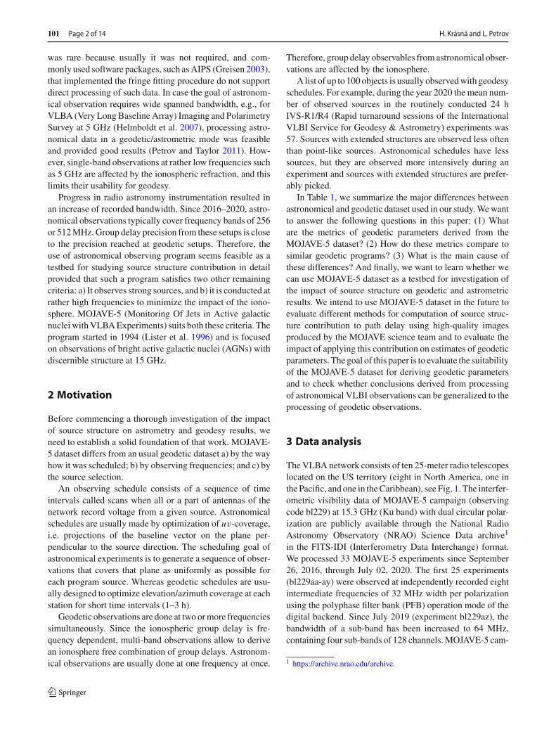
TheVLBAnetwork consists of ten 25-meter radio telescopeslocated on the US territory (eight in North America, one inthe Pacific, and one in theCaribbean), see Fig. 1. The interfer-ometric visibility data of MOJAVE-5 campaign (observingcode bl229) at 15.3 GHz (Ku band) with dual circular polar-ization are publicly available through the National RadioAstronomy Observatory (NRAO) Science Data archive1

in the FITS-IDI (Interferometry Data Interchange) format.We processed 33 MOJAVE-5 experiments since September26, 2016, through July 02, 2020. The first 25 experiments(bl229aa-ay) were observed at independently recorded eightintermediate frequencies of 32 MHz width per polarizationusing the polyphase filter bank (PFB) operation mode of thedigital backend. Since July 2019 (experiment bl229az), thebandwidth of a sub-band has been increased to 64 MHz,containing four sub-bands of 128 channels.MOJAVE-5 cam-

1 https://archive.nrao.edu/archive.

123

VLBA campaign MOJAVE for geodesy Page 3 of 14 101

Table 1 Overview of major differences between the astronomical dataset MOJAVE-5 bl229 and the geodetic dataset RV&CN

MOJAVE-5 bl229 RV&CN

Optimization of uv-coverage Sky coverage

Number of observed frequencies One Two

Preferable observed sources With extended structure Point-like

Number of sources Less sources observed intensively More sources with less observations

180˚

180˚

−120˚

−120˚

−60˚

−60˚

45˚ 45˚

Fig. 1 Distribution of the ten VLBA radio telescopes

Table 2 Lower edge frequencyof the sub-bands in theMOJAVE-5 bl229 experimentsin GHz

bl229aa–ay bl229az–bg

15.22400 15.17575

15.25600 15.25575

15.28800 15.31975

15.32000 15.38375

15.35200

15.38400

15.41600

15.44800

paign has used four IFs of 64 MHz width per polarizationusing the direct digital converter (DDC) operation modeof the digital backend, also known as DDC personality. Inboth cases, the total recorded bandwidth per polarization is256 MHz (see Table 2).

We processed the observations with the fringe-fitting soft-ware PIMA (Petrov et al. 2011b) running coarse fringefitting—bandpass calibration—fine fringefitting andproduc-ing the output databases that include group delays and theiruncertainties among other parameters. These quantities serveas input for the data analysis software package pSolve2 andVieVS (Böhm et al. 2018).

As a reference dataset, we analyzed 28 geodetic RV (reg-ular geodesy with VLBI) (Petrov et al. 2009) and 6 CN(concurrent with even IVS-R1) dual-band sessions observedat 2.3/8.6 GHz (S/X bands) for the same time span start-ing with rv119 on September 14, 2016, through July 07,

2 http://astrogeo.org/psolve.

2020. The RV network consists of the ten VLBA stationsplus up to seven other geodetic stations ensuring global geo-graphic coverage. These sessions are designed to provideaccurate estimates of the Earth orientation parameters (EOP),a highly accurate terrestrial reference frame (TRF) deter-mination, and source position estimation where the VLBAstations are incorporated into the VLBI reference framethrough the inclusion of other geodetic stationswith long his-tory of observations. In CN experiments, only the ten VLBAstations participate (Thomas and MacMillan 2020).

To assess the quality of geodetic results, we estimatedbaseline lengths and EOP and computed their weighted rootmean squares (wrms) from the astrophysicalMOJAVE-5 pro-gram and dedicated geodetic RV&CN experiments. As anextra check, we analyzed the VLBA data in several ways.One solution was produced using the software PIMA for thefringe fitting and pSolve for the analysis. In the second solu-tion, we analyzed group delays produced with PIMA withthe geodeticVLBI analysis softwareVieVS. For theRV&CNexperiments, we run another solution with VieVS where weused group delays obtained from Fourfit visibility analysissoftware (Cappallo 2017). The latter data products in vgosDBformat were retrieved from the IVS data archive.3 Table 3contains the parameterization of the solutions in pSolve andVieVS, respectively. Table 4 shows weighted rms of post-fitresiduals. TheMOJAVE-5 andRV&CNexperiments are pro-cessed in the same manner with the same parameterizationto allow an informative comparison.Baseline length repeatability. We ran several solutions, andwe compared the scatter in baseline length estimates. Weshow in Fig. 2 the wrms of the estimated VLBA baselinelengths from solutions computed with pSolve (left panel)and with VieVS (right panel). Red crosses denote the base-lines determined from the MOJAVE-5 experiments in bothplots. We show in the left plot of Fig. 2 the baseline scat-ter computed from the RV&CN sessions with the wholescheduled network (blue x-signs) and with observations con-ducted at the VLBA stations only (green diamonds). Theplot demonstrates that dropping the data obtained with non-VLBA stations does not change the wrms of the baselinelengths between the VLBA telescopes significantly. In thewhole dataset of RV&CN sessions, 82% of observations was

3 Available at https://ivscc.gsfc.nasa.gov/products-data.

123

101 Page 4 of 14 H. Krásná and L. Petrov

Table 3 Parameterization of estimated parameters of a single session solution in pSolve and VieVS

pSolve

CRF fixed to ICRF3 with exception of sources having the χ2/nd f > 1.5

TRF NNT/NNR condition w.r.t. ITRF2014 on VLBA stations with 0.1 mm constraints

ERP Offset and rate without constraints

Celestial pole offsets Offset without constraints

Zenith wet delay B-spline with time span 20 min and sigma of constraints 50 ps/h

Tropo. gradients B-spline with time span 8 h with sigma of constr. 0.5 mm on offset and 2.00 mm/day on rate

Clocks B-spline with time span 1 h and constraint sigma 5.e-14 s/s

Baseline clock offsets Offset with constraint sigma 500 ns

VieVS

CRF Fixed to ICRF3 with exception of sources identified with pSolve

TRF NNT/NNR condition w.r.t. ITRF2014 on VLBA stations

ERP Piecewise linear offsets (pwlo) with time interval 24 h with relative constraints 1 mas

Celestial pole offsets pwlo with time interval 24 h with relative constraints 0.1 μas

Zenith wet delay pwlo with time interval 30 min with relative constraints 50 ps between intervals

Tropo. gradients pwlo with time interval 3 h with relative constraints 5 mm between intervals

Clocks pwlo with time interval 1 h with relative constraints 43 ps between intervals, one rate and quadratic term

Baseline clock offsets Offset without constraints

The statistic value χ2/nd f stands for ratio of the sum of squares of the weighted residuals over the used observations of the specific source to itsmathematical expectation

carried out at baselines with VLBA—VLBA antennas. 14%of observations was conducted with one non-VLBA and oneVLBA antenna, and 8% of observations was realized withnon-VLBA antennas. In both solutions (with and withoutnon-VLBA stations), the NNT/NNR condition was appliedto VLBA antennas only. In the right plot of that figure, wecompare theMOJAVE-5 bl229 baseline scatterwithRV&CNsessions processed with Fourfit. We got approximately thesame baseline length scatter from MOJAVE-5 and RV&CNsessions using totally independent software packages. Thenegligible differences in results from pSolve and VieVS givethe confidence that an error in data analysis did not happen.

There is an increase in the baseline length repeatabilityfrom a solution using the MOJAVE-5 dataset with respect tothe reference RV&CN sessions. The baseline length repeata-bility differences derived from RV&CN and MOJAVE-5 areabout 1.3 mm at a 1000 km long baseline and 3.2 mm atthe 8611 km baseline length. The coefficients of the linearregression are summarized in Table 5. We conclude that thebaseline length repeatability derived from analysis of single-band 15 GHz MOJAVE-5 experiments is approximately afactor of 1.5 larger than the repeatability derived from thecontemporary dual-band 2.3/8.6 GHz geodetic dataset.Earth orientation parameters The Earth orientation parame-ters were estimated in a so-called backward solution, i.e. ina solution consistent with globally estimated terrestrial andcelestial reference frames from the processed sessions. Theorientation and the origin of the TRF are set to have no-net-translation (NNT) and no-net-rotation (NNR) with respect

Table 4 Weighted rms of post-fit residuals in ps

Min Max Median

MOJAVE-5 bl229 11.3 28.7 18.4

RV&CN VLBA only 14.7 37.8 24.1

RV&CN all stations 14.7 40.3 25.2

Table 5 Parameters of the fitted linear regression model of baselinelength repeatability in the form a · L + b where L is length of baselinein mm

Dataset Software a [ppb] b [mm]

MOJAVE-5 bl229 PIMA, pSolve 0.91 2.50

RV&CN VLBA only PIMA, pSolve 0.64 1.51

RV&CN all stations PIMA, pSolve 0.61 1.54

MOJAVE-5 bl229 PIMA, VieVS 0.98 2.04

RV&CN all stations Fourfit, VieVS 0.60 1.17

to ITRF2014 (Altamimi et al. 2016) for positions of all tenVLBA stations, and the CRF is oriented by imposing the no-net-rotation condition with respect to ICRF3 (Charlot et al.2020) coordinates of 26 observed defining sources. We ranseveral solutions similar to those we introduced in the pre-vious paragraph, and we computed the EOP with softwarepackage pSolve. Table 6 shows the wrms of the ERP (polarmotion components and dUT1)w.r.t. IERS 14C04 (Bizouardet al. 2019) time series after a trend and bias removal,whereasthe wrms of the celestial pole offsets is given w.r.t. a har-

123

VLBA campaign MOJAVE for geodesy Page 5 of 14 101

0 2 4 6 8

baseline length [1000 km]

0

5

10

15w

rms

[mm

] MOJAVE-5 bl229RV&CN all stationsRV&CN VLBA only

0 2 4 6 8

baseline length [1000 km]

0

5

10

15

wrm

s [m

m] MOJAVE-5 bl229

RV&CN vgosDB

Fig. 2 Baseline length repeatability at the VLBA network. Left panelcompares baseline scatter computed with pSolve from MOJAVE-5dataset (red crosses), RV&CN dataset after processing data from allstations (blue x-signs), and RV&CN dataset when non-VLBA obser-

vations were dropped (green diamonds). Right panel shows baselinelength repeatability computedwithVieVS fromMOJAVE-5 dataset (redcrosses) and RV&CN dataset processed with Fourfit (brown circles)

Table 6 Wrms and median formal error statistics of the estimated EOP from MOJAVE-5 bl229 and RV&CN series

x-pole [μas] y-pole [μas] dUT1 [μs] dX [μas] dY [μas]

MOJAVE-5 bl229 wrms 228 286 23 169 128

Median formal error 109 153 9 59 56

RV&CN VLBA only wrms 126 218 15 89 129

Median formal error 80 120 6 92 69

RV&CN all stations wrms 117 130 14 72 87

Median formal error 57 89 4 86 60

The values for ERP are given w.r.t. IERS 14 C04 time series after trend and bias removal. The celestial pole offsets differences dX and dY werecomputed with respect to the empirical harmonic expansion heo_20200606.heo

monic expansion heo_20200606.heo produced from analysisof available geodetic VLBI data since 1980 through 2020using the method presented in Petrov (2007). In addition, themedian formal error for all five EOP is summarized in thetable. We show three solutions computed with pSolve sim-ilar to those introduced by the baseline length repeatability,i.e., EOP from MOJAVE-5 dataset, EOP from RV&CN ses-sions including all stations, and EOP from RV&CN sessionsusing the VLBA telescopes only. Estimation of EOP usingsingle band observations at high frequencies was made inthe past (e.g., Petrov et al. 2011a). Our recent processingof 37 VLBA experiments at 24 GHz (Krásná et al. 2019)showed that although formal uncertainties were on par withdual-band regular geodetic experiments (60 μas for x-pole,80 μas for y-pole and 5 μs for UT1), the wrms of the dif-ference with respect to the IERS 14 C04 time series taken asa reference were larger than formal uncertainties by a factorof three for polar motion and a factor of ten for UT1. Table 6shows that ERP determined from MOJAVE-5 data have thewrms differences with respect to the reference IERS C04 14by a factor of 1.3 to 1.8 larger than fromRV&CNexperimentsat the same network.

4 Differences betweenMOJAVE-5 bl229 andRV&CN

We recognize there are three major differences between thedatasets which may have an impact on geodetic results. First,

modeling of the ionospheric path delay was different sinceMOJAVE-5 was observed at a single band. Second, differentscheduling approacheswere used due to different goals of theexperiments. Third, different radio sources were selected forobservations. We isolate these factors and determine whichfactor has the largest impact on the accuracy of geodeticsolutions.

4.1 Ionosphere

The ionosphere is a refractivemedia. Propagating in the iono-sphere, phase delay decreases and group delay τgr increaseswith respect to the ionosphere-free τi f group delay in theabsence of the ionosphere as

τgr = τi f + κΔTEC/ f 2eff , (1)

where feff is the effective frequency that is within severalpercent of the recorded central sky frequency, ΔTEC is thedifferential Total Electron Content measured in TEC units(TECU, 1 TECU = 1016 electron/m2):

ΔTEC =∫

Nv ds1 −∫

Nv ds2 (2)

123

101 Page 6 of 14 H. Krásná and L. Petrov

with s1 and s2 as paths of wave propagation from a source tothe first and second station of the radio interferometer, and

κ = 10−16 · e2

2 cme εo= 5.308018 × 1010 s−1 (3)

where e—charge of an electron, me—mass of an electron,εo—permittivity of free space, and c—velocity of light invacuum.

To mitigate the impact of the ionosphere on group delay,geodetic observations are usually conducted at two frequen-cies simultaneously. Combining group delays τu and τl at theupper and lower frequencies fu and fl , respectively, we canderive the differential TEC, the ionosphere-free path delay,and the ionospheric contribution in the upper band τiu as

ΔT EC = f 2u f 2lf 2u − f 2l

(τl − τu),

τi f = f 2uf 2u − f 2l

τu − f 2lf 2u − f 2l

τl ,

τiu = f 2lf 2u − f 2l

(τl − τu). (4)

Derivations of these equations can be found, for example,in Petrov et al. (2011b). This approach allows to effectivelycancel the ionospheric contribution, leaving residual contri-bution at a level not exceeding several picoseconds (Hawareyet al. 2005).

MOJAVE-5 program used only one frequency. An alterna-tive approach for modeling the ionospheric contribution is touse TEC maps from GNSS observation processing. Apply-ing time and spatial interpolation, we can compute TEC inthe vertical direction for each station and each observation.Then, we can relate the TEC in the direction of observation atthe elevation angle E to the TEC in the vertical direction viaa mapping function Mi (E). Considering the ionosphere as athin shell at height H , we can easily derive the ionosphericmapping function as

Mi (E) = 1

cosβ(E),

β(E) = arcsincos E

1 + HR⊕

, (5)

where R⊕ is the Earth’s radius.We used Center for Orbit Determination in Europe

(CODE) TEC time series (Schaer 1999)4 with a resolutionof 5◦ × 2.5◦ × 2h . This resolution is relatively coarse andaccounts only for a part of the signal. Therefore, our results

4 Available at ftp://ftp.aiub.unibe.ch/CODE.

of processing MOJAVE-5 observations are affected by sys-tematic errors caused by the residual ionosphere.

In order to quantify the residual ionospheric signal, weprocessed the dual-band RV&CN data set. For the purpose ofthis study, we consider that the ionospheric-free linear com-bination of X and S band group delays has no ionosphericcontribution. We can form the differences between the iono-spheric contribution computed from TEC maps and from Xand S band group delays and investigate the properties interms of a stochastic process.

Solving for zenith path delays in the neutral atmospherewill pick up a portion of the slowly varying bias, but theionospheric fluctuations at scales less than several hourswill propagate to residuals. However, we can characterizestochastic properties of the residual signal similar to theapproaches developed in Petrov et al. (2011b, 2019) andPetrov (2021). The ionospheric path delay fluctuation is anon-stationary process. We can expect that fluctuations atscales x will be related to fluctuations at scales y via a powerlaw from the general results of the turbulence theory (seeTatarskii 1971). Therefore, we did the following:

First, we computed themean differences of dgv = τig−τivbetween the ionospheric path delay at X band computed fromTEC maps (τig) and from VLBI dual-band observables (τiv)for every baseline and every experiment in the RV&CN dual-band dataset, and then, we subtracted the mean value fromdgv . Themean value is the sumof the bias betweenTECmapsand VLBI ionospheric path delay and a constant instrumen-tal delay in VLBI hardware. Since the constant instrumentaldelay that may be even larger than the ionospheric signal isnot calibrated, the mean value of dgv is meaningless. Then,we computed the rms over dgv . We discarded the data withclock jumps that may happen at only one band. We got timeseries of rms(dgv), and we examined empirical relationshipsof rms(dgv) with other statistics. We found that rms2(dgv)has a linear dependence on rms(τig). The power law depen-dence between dgv and τig was expected, but the power lawcoefficient, 2, is purely empirical. Figure 3 demonstrates thetime series of dgv and their fit.

We can compute the rms of the ionospheric errors at agiven baseline of a given experiment via

rms(dgv) =√

ρ rms(τig), (6)

where ρ is the empirical coefficient determined from fitting(see Fig. 3) equal to 12.8 ps and the rms is expressed in ps.This empirical relationship allows us to predict the secondmoment of the residual noise after we perform data reductionfor the ionospheric contribution using TEC maps. One canexpect that if the TEC variance is greater, the residual errorsare also greater. Expression (6) quantifies this dependence.

123

VLBA campaign MOJAVE for geodesy Page 7 of 14 101

Fig. 3 The rms of the errors in the ionospheric path delay as a functionof the rms of the variations of the ionospheric group delays derivedfrom TEC maps (green dots). The solid blue line shows a regression ina form of the power law 1/2

We have computed baseline-dependent additive noise dueto mismodeled ionosphere for every baseline and everyexperiment of MOJAVE-5 program using τig . We addedthat noise to the a priori group delay errors in quadratureand computed new weights. We ran several baseline solu-tions, computed baseline repeatabilities, and compared themwith the reference dual-band solution using RV&CN data. Insolution “bx,” we used the ionosphere-free combinations ofgroup delays, added the contribution of the ionosphere τiu tothem, and processed these data the same way as MOJAVE-5 data, i.e., performing data reduction for the ionosphereusing CODE TEC maps and inflating a priori group delayuncertainties for the additional noise due to mismodeling theionosphere. In the second solution “bu,” we simulated howthe deficiencyofCODETECmodelwould have impacted ourRV&CN solution, as if these experiments ran at 15.3 GHzinstead of 2.3/8.6 GHz. To achieve this, we re-scaled τiuby the square of the frequency ratio (8.64/15.28)2 ≈ 0.32.Figure 4 shows a fit in the form

√(a L)2 + b2 for all these

solutions. The baseline length repeatability fromMOJAVE-5solution is shown by the dashed line.

We found that the impact of the mismodeled ionosphereon the baseline length repeatability of VLBA data collectedin 2016–2020 at 15.3 GHz during Solar minimum is negligi-ble. Therefore, an increase in the baseline length repeatabilityfrom a geodetic solution using the MOJAVE-5 dataset withrespect to the reference dual-band RV&CN solution can-not be explained by the unaccounted contribution of theionosphere. This result should not be extrapolated to otherestimated parameter, such as source position, and should notbe extrapolated to epochs of the Solar maximum.

4.2 Scheduling

Scheduling of a VLBI experiment is a complex task. Thescheduler has to evaluate several criteria which lead to the

Fig. 4 The dependencies of the baseline length repeatability fits onthe baseline length. The upper blue curve shows the baseline repeata-bility for the X band only in the “bx” solution that uses GNSS TECmaps. Two lower very close curves, red and green, show the baselinelength repeatability for the “bu” solution that demonstrates the effectof mismodeled ionosphere on Ku band observable, and the referencedual-band solution. The dashed black line shows the baseline lengthrepeatability from the MOJAVE-5 solution

best schedule according to the focus of the current experi-ment.The major criteria for design of the geodetic schedule are thesky coverage over the individual stations, number of obser-vations, and scan duration. The general scheduling conceptof the established software sked for the geodetic sessions canbe found in Gipson (2010). Evenly distributed observationsover all elevation angles at a given station ensure a gooddecorrelation of station dependent parameters such as sta-tion height, zenith wet delay, clock parameters, or baselineclock offsets (e.g., Nothnagel et al. 2002), and therefore, suchschedule can be regarded as station-centric. A large numberof observations in general improves the accuracy of the esti-mated geodetic parameters due to higher redundancy. Thechallenge for the scheduling software is to find the best com-promise between a) the long antenna slew time needed forthe best sky coverage in a short interval (1–3 h) allowing ahigh time resolution of the estimated parameters and b) theshort antenna slew time allowing for a high number of obser-vations with sufficient scan duration and high signal-to-noiseratio.Astronomic VLBI schedules are mainly scheduled usingSched (Walker 2020). The primary goal of the MOJAVE-5bl229 experiments is to provide best images of jets in activegalactic nuclei. Therefore, their schedule is optimized to tracka small set of sources (30) in a 24-h session in ten scans persource for a total on-source time of ∼ 35 minutes. A givensource is scheduled to have at least six antennas providing

123

101 Page 8 of 14 H. Krásná and L. Petrov

0

30

60

90

120

150

180

210

240

270

300

330

30

60

90

BR-VLBA

00h

06h

12h

18h

24h0

30

60

90

120

150

180

210

240

270

300

330

30

60

90

FD-VLBA

00h

06h

12h

18h

24h0

30

60

90

120

150

180

210

240

270

300

330

30

60

90

SC-VLBA

00h

06h

12h

18h

24h

0

30

60

90

120

150

180

210

240

270

300

330

30

60

90

BR-VLBA

00h

06h

12h

18h

24h0

30

60

90

120

150

180

210

240

270

300

330

30

60

90

FD-VLBA

00h

06h

12h

18h

24h0

30

60

90

120

150

180

210

240

270

300

330

30

60

90

SC-VLBA

00h

06h

12h

18h

24h

Fig. 5 Sky coverage at three VLBA stations: BR-VLBA, FD-VLBA, and SC-VLBA during the bl229bc MOJAVE-5 experiment (upper plots) andthe cn1924 experiment (lower plots)

observations of larger than 10◦ elevation.5 Such schedule isconsidered as source-centric.In Fig. 5, we show the sky coverage during a 24-h observingsession at three selected telescopes (BR-VLBA, FD-VLBA,and SC-VLBA) where colors depict the time passed sincethe session start. As an example, we show the sky cov-erage during the MOJAVE-5 session bl229bc observed onDecember 22, 2019, in the upper plots and the cn1924session observed with the same network on December 09,2019, in the lower plots. Table 7 summarizes the averagenumber of scans in a 24-h experiment at each of the tenVLBA telescopes computed over the investigated time period(September 2016–July 2020). We see that about twice thenumber of scans at each telescope was observed in thegeodetic experiment with shorter integration time than inMOJAVE-5 observing sessions that used longer integrations.Figure 6 presents the total number of observed sources ineach session (upper plot) and the median number of observa-tions during a 24-h session for each source computed over therespective four-year period. The median number of observedradio sources is 30 inMOJAVE-5 sessions, and 78 inRV&CNsessions. Comparison of the number of observations for eachsource during a whole session shows that 95% of the AGNsobserved in MOJAVE-5 sessions have more than 150 obser-

5 http://www.physics.purdue.edu/astro/MOJAVE/data.html.

vations, whereas only 35% of the sources were observedin RV&CN that often. Our results confirm that geodeticschedules are designed to provide a good sky coverage foreach station and the sources are picked up to improve theazimuth/elevation coverage regardless of how often they areobserved in a given experiment.

4.3 Simulations

To touch the effect of source structure, we run simulations ofthe observations. Using the simulation VieVS tool Vie_SIM(Pany et al. 2011), we replaced group delay observables withsynthetic artificial groupdelays providedby the randomnoisegenerator as

τgr = τmod + (τclk + τzwd + τ f l). (7)

Weadded three stochastic error sources to the theoreticallycomputed time delay (τmod ): delay caused by the turbulencein the troposphere (τzwd ), station clock (τclk), and the Gaus-sian noise (τ f l ) with σ=20 ps that accounts for the thermalnoise and instrumental errors. We used the model of Nilssonet al. (2007) for simulation of zenith wet delay implementedin VieVS. In the framework of that approach, we consid-ered that the atmospheric turbulence for every station isdescribed with a structure function with the refractive index

123

VLBA campaign MOJAVE for geodesy Page 9 of 14 101

Table 7 Mean number of scansat VLBA telescopes in onesession computed over theperiod of interest (September2016–July 2020)

Br Fd Hn Kp La Mk Nl Ov Pt Sc

MOJAVE-5 bl229 series 245 245 241 248 251 204 251 252 235 219

Geodetic RV&CN experiments 451 485 445 493 483 357 467 487 451 423

2017 2018 2019 2020

20

40

60

80

no. o

f sou

rces

-90° -45° 0 45° 90°declination

0

200

400

600

no. o

f obs

erva

tions

Fig. 6 The upper plot shows the number of observed sources in eachsession. The lower plot depicts the median number of observations foreach source. The red crosses stand for the bl229 experiments and bluex-signs for the RV&CN experiments

structure constant Cn = 1.8 × 10−7 m−1/3, the effectiveheight H = 2 km, and the constant wind velocity v = 8 m/stoward east. For the simulations, we computed the covariancematrix between group delays for each pair of observations ofa given station and used them for computation of the fullweight matrices under an assumption that the atmosphericturbulence is a stationary process. The simulation of stationclocks was performed with an Allan standard deviation of1 · 10−14 at 50 min. We did not include modeling sourcestructure into simulation.

We have computed baseline length repeatabilities fromsimulated RV&CN and MOJAVE-5 datasets. The regressionlines in a form a · L + b for simulated and real data areshown in Fig. 7. We see from these plots that simulationresults show even larger disparity in repeatabilities betweenMOJAVE-5 and RV&CN data than we saw in real obser-vations. We should note that τclk and τ f l in equation (7) areexactly the same for both datasets, and τzwd that is dependenton elevations and time is similar in both datasets because itwas derived from the same model. Therefore, the stochas-tic model we used for MOJAVE-5 and RV&CN simulationsis essentially the same. This finding pinpoints the origin ofdiscrepancies in the results obtained by processing real data:differences in schedules.

Since atmospheric path delays and clock functions aremodeled in a form of an expansion over the B-spline basis

0 2 4 6 8

baseline length [1000 km]

0

5

10

15

wrm

s [m

m]

Fig. 7 The wrms of baseline length from real (dashed line) and sim-ulated observations (solid line). The upper red lines show the baselinelength repeatability from analysis and simulation of MOJAVE-5 data.The low blue lines show results of analysis and simulation of RV&CNdata

Table 8 The wrms of the simulated EOP from MOJAVE-5 bl229 andRV&CN experiments observed with the VLBA network. The values aregiven w.r.t. the IERS 14 C04 time series after trend and bias removal

x-pole y-pole dUT1 dX dY[μas] [μas] [μs] [μas] [μas]

MOJAVE-5 bl229 158 225 16 82 98

RV&CN VLBA only 118 184 10 82 97

with a time span of 20–60 minutes, in order to decorrelatethese two groups of nuisance parameters and the stationvertical component, observations at significantly differentelevations are required. Figure 8 shows that the spread ofobservations over mapping function (approximately recip-rocal to sine of elevation angle which equals the partialderivative of the time delay w.r.t. zenith wet delay) for thegeodetic experiment rv119 is noticeably wider and observa-tions at elevations below 30◦, which corresponds to mappingfunction > 2, appear more often than in the astronomicalexperiment bl229aa.

In order to look at the problem in more detail, we inves-tigated correlations between estimates of the vertical siteposition and atmospheric path delays. From the real data,we computed the median correlation coefficient − 0.22 forRV&CN sessions and− 0.35 for MOJAVE-5 sessions. Sincethese numbers depend on the elevation angles of the observa-tions, we considered the cosine of the median elevation angleas a factor. Themedian elevation angle over all sessions in thedataset is 33◦ for RV&CN and 47◦ for MOJAVE-5. There-fore, the multiplication of the median correlation coefficientwith this factor brought the reduced median correlation coef-ficients closer together, i.e. − 0.18 for RV&CN sessions and-0.24 for MOJAVE-5. We ran a series of solutions using

123

101 Page 10 of 14 H. Krásná and L. Petrov

Fig. 8 The distribution of observations over the mapping function forstation LA-VLBAwithin first two hours of an experiment. Since devia-tion of the mapping function from 1/sin(elevation) is small at elevations

above 10 deg, mapping function 1/sin(elevation) is used here for illus-trative purpose. Left: geodetic experiment rv119. Right: astronomicalexperiment bl229aa

RV&CN data and flagged out observations below a certainelevation angle. Table 9 summarizes the findings.An increasein the elevation cutoff results in an increase in the baselinelength repeatability. MOJAVE-5 has few observations belowelevations 30◦ and none below 20◦. The achieved baselinelength repeatability from MOJAVE-5 experiments is similarto the repeatability from RV&CN experiments when obser-vations below 20–25◦ are not included in a solution.Figure 9 shows individual correlation coefficients in simu-latedgeodetic experiment cn1924 for cutoff elevation3◦, 20◦,and 30◦. The median correlation coefficient between verti-cal displacement and clock offset at the respective station is0.19, 0.27, and 0.39 for the increasing cutoff elevation angle.The median correlation coefficient between vertical compo-nent and a residual atmospheric zenith path delay is− 0.37,−0.64, and− 0.79when the elevation cutoff is increasing. Thisproves that the strategy including radio sources under lowele-vations in the schedule over short periods of time allows todecorrelate station dependent parameters in the data analysisand to provide better baseline length repeatability.We also investigated the residual EOP estimates from thesimulated RV&CN and MOJAVE-5 datasets with respect tothe IERS C04 14 time series taken as a reference. The resultsof this simulation are presented in Table 8. The simulationresults confirm about the same disparity of 20-60% of thewrms fromMOJAVE-5 and RV&CN dataset as in the resultsderived from real observations (compare with Table 6).

4.4 Insight into a possible contribution of the sourcestructure to the baseline length

The first indicator of astrometric source quality based onsource structure corrections was developed by Fey and Char-lot (1997). They derived the so-called structure index (SI)from VLBI source images as the median value of the groupstructure delay (τstr ) determined for pixels in a 512×512 uv-grid for all baselines shorter than the diameter of the Earth.Figure 10 shows images of the three most observed sources

Table 9 The coefficients of the baseline length repeatability regressionin a form of a · L + b as a function of elevation angle from processingRV&CN VLBA observations

Elevation cutoff a [ppb] b [mm]

0◦ 0.55 1.46

5◦ 0.55 1.46

10◦ 0.70 1.35

15◦ 0.90 1.14

20◦ 1.09 1.14

25◦ 1.22 1.14

30◦ 1.86 1.49

parameter pair-1

-0.5

0

0.5

corre

latio

n co

effic

ient

Fig. 9 Correlation coefficients in simulated geodetic experimentcn1924 for cutoff elevation 3◦ (blue x-signs), 20◦ (green circles),and 30◦ (pink crosses). The order of parameter pairs at the x-axis: (1st–9th): station’s vertical component and clock offset for all stations exceptof the clock reference; (10th–last): station’s vertical component and aresidual atmospheric zenith path delay (estimated as pwlo every hour)for all ten stations (the solid line connects coefficients that belong to thesame station)

in the first session of each dataset. In the session bl229aa,these sources are 0636 + 680, 0210 + 515, and 0128 + 554;in the session rv119, the most observed sources are 2229 +

123

VLBA campaign MOJAVE for geodesy Page 11 of 14 101

Fig. 10 Images of three most observed sources (0636 + 680 with SI2, 0210 + 515 with SI 3, and 0128 + 554 with SI 4) in the bl229aaMOJAVE-5 experiment (upper plots) and in the rv119 experiment at Xband (lower plots: 2229 + 695 with SI 2, 0345 + 460 with SI 2, 0529+ 483 with SI 2). We have produced images from rv119 ourselves. The

images in FITS format are available in the Astrogeo VLBI FITS imagedatabase http://asteogeo.org/vlbi_images. Information about the struc-ture index for the X band sources was taken from the Bordeaux VLBIImage Database available at http://bvid.astrophy.u-bordeaux.fr

695, 0345 + 460, and 0529 + 483. We computed the SI for allsources observed in bl229aa. For that calculation, we usedmaps provided byMOJAVE team6 and split the sources in thefour SI groups according to the median value of calculatedstructure delay corrections. Among 30 sources observed inbl229aa, 3 sources have SI 1, 14 sources SI 2, 8 sources SI 3,and 5 sources have the highest SI 4.

We compared the post-fit residuals in session bl229aafrom real observations vreal (upper plots) and from simu-lated observations vsim (lower plots) as shown in Fig. 11. Asan example, we highlighted the most observed source 0636 +680 in this sessionwhich has structure index 2 and 0128+554with structure index 4. The comparison shows that the scatterof delay residuals for 0636 + 680 is similar to real and sim-ulated observations and the rms reaches 29.6 ps and 29.3 ps,respectively. The rms of delay residuals of source 0128 +554 with extended structure is 2.5 times larger when com-puted from real observations compared to simulated ones,72.3 ps and 27.4 ps, respectively. We computed the rms ofdelay residuals for every source in the bl229aa experiment

6 Available at https://www.physics.purdue.edu/MOJAVE.

and built the difference between the rms from real and sim-ulated observations. The median value of the rms differencewas calculated as

Δrmsmed = med(rms(vreal) − rms(vsim)) (8)

over each source group with respect to the structure index.The obtained median values are summarized in Table 10.We see that the difference between simulated and real delayresiduals is raising with an increasing source structure indexsince the structure group delay is not modeled in the simu-lated observations. With the SI 1 taken as reference, the rmsof the delay residuals increases by about 36 ps for sourceswith SI 4. The lower wrms of post-fit residuals from pro-cessing real observations compared to the simulated ones forsources with low structure indices (SI 1 and SI 2) is mani-fested by the negative Δrmsmed. It is due to the fact that therandom Gaussian noise with the rms of 20 ps that had beenadded to simulated path delay in our simulation is too highfor these compact sources.

We see that the source structure contribution increasesthe rms of the post-fit residuals, but such an increase even

123

101 Page 12 of 14 H. Krásná and L. Petrov

-200

-100

0

100

200[p

s]0636+680

57657.25 57657.50 57657.75 57658 57658.25BL229aa 2016-09-26 [mjd]

-200

-100

0

100

200

[ps]

-200

-100

0

100

200

[ps]

0128+554

57657.25 57657.50 57657.75 57658 57658.25BL229aa 2016-09-26 [mjd]

-200

-100

0

100

200

[ps]

Fig. 11 Post-fit residuals in session bl229aa for real (upper plots) and simulated (lower plots) observations. Highlighted are sources 0636 + 680with SI 2 on the left and 0128 + 554 with SI 4 on the right

Table 10 Median of rms differences Δrmsmed between delay residualsfrom real and simulated observations in bl229aa. Sources are dividedin four groups according to their structure index, i.e. according to theirmedian group structure delay med(τstr ). Nsou stands for number ofsources in the group

SI med(τstr ) [ps] Nsou Δrmsmed [ps]

1 0–3 3 − 11.3

2 3–10 14 − 6.6

3 10–30 8 9.0

4 30–∞ 5 25.0

for a subset of sources with strong radio jets picked up foran astronomical program does not have a noticeable impacton baseline length repeatability. Source structure causes notonly random but also systematic errors, but their impact onthe baseline length repeatability is insignificant. We exercisea caution to generalize this result to source position estimates.This requires a further investigation that is beyond the scopeof present work.

5 Conclusions

We have processed 33 diurnal astronomical observing VLBIsessions at 15GHzunder programMOJAVE-5 and 34 diurnalVLBI geodetic dual-band observing sessions at 2 and 8 GHzunder programs RV and CN. Both observing sessions ran atthe same ten-station VLBA network with baseline lengths ina range from 237 to 8612 km at approximately the same timeinterval 2016.7–2020.5.

We found that while the median wrms of post-fit residu-als fromMOJAVE-5 programwas lower than from RV&CN,

18.4 ps versus 24.1 ps, important metrics of the geodeticquality of solutions, such as baseline length repeatability andwrms of the differences of the ERP with respect to the refer-ence IERS C04 times series, were a factor 1.3 to 1.8 worse.We investigated the origin of these discrepancies. We haveestablished that modeling the ionospheric path delay usingthe GNSS TEC maps was adequate for processing 15 GHzdata during the Solar minimum, and the errors of these TECmaps did not affect baseline length repeatability at a notice-able level. We investigated whether the source structure canbe a factor, since MOJAVE-5 targeted objects with strongradio jets and we have not found evidence it affected baselinelength repeatability. Finally, we ran solutions with simulatedright hand sides for bothMOJAVE-5 and RV&CN programs.The stochastic model used for these simulations was almostthe same. We were able to reproduce discrepancies in base-line lengths and EOP time series statistics.

We have established that the major factor that causes dis-crepancies in baseline length repeatability is a more agileschedule of RV&CN experiments that includes more scansat low and high elevations at short time intervals 1–3 hthan astronomical experiments. We showed that the correla-tion coefficients between the station vertical component andatmospheric zenith path delay increase with an increasingelevation cutoff angle.Whenwe removedobservations below20–25◦ elevations in RV&CN, we got a similar repeatabilityas in MOJAVE-5 program.

Although the use of single-band astronomical VLBI datafrom MOJAVE-5 program for geodesy provided less accu-rate results than the use of VLBI data from the dedicatedgeodesy RV&CN campaign, the baseline length repeatabil-ity is still below 1 ppb. This gives us a good estimate of theimpact of remaining systematic errors that are specific for

123

VLBA campaign MOJAVE for geodesy Page 13 of 14 101

MOJAVE-5.This very low level of systematic errors confirmsthat MOJAVE-5 dataset is an excellent testbed for investi-gation of the effect of source structure on astrometry andgeodesy in full detail.

Acknowledgements The constructive comments from three anony-mous reviewers are highly appreciated. HK worked within the HerthaFirnberg position T697-N29, funded by the Austrian Science Fund(FWF). LP work was supported by the NASA Earth Surface and Inte-rior program, project 19-ESI19-0030. This research has made use ofdata from the MOJAVE database that is maintained by the MOJAVEteam (Lister et al. 1996). TheVeryLongBaselineArray (VLBA) is oper-ated by the National Radio Astronomy Observatory, which is a facilityof the National Science Foundation, and operated under cooperativeagreement by Associated Universities, Inc. The authors acknowledgeuse of the VLBA under the US Naval Observatory’s time allocation.This work supports USNO’s ongoing research into the celestial refer-ence frame and geodesy.

Author contributions HK and LP designed the research, performedthe calculations, and interpreted the results; HK wrote the paper withsupport byLP.Both authors approved thefinal versionof themanuscript.

Funding Open access funding provided by TU Wien (TUW).

Data Availability Statement All observation data were retrieved frompublicly available database https://archive.nrao.edu/archive. The TECtime series was downloaded from ftp://ftp.aiub.unibe.ch/CODE. Soft-ware packages which are necessary to reproduce the results are openaccess and can be downloaded from http://astrogeo.org and https://github.com/TUW-VieVS/.

Open Access This article is licensed under a Creative CommonsAttribution 4.0 International License, which permits use, sharing, adap-tation, distribution and reproduction in any medium or format, aslong as you give appropriate credit to the original author(s) and thesource, provide a link to the Creative Commons licence, and indi-cate if changes were made. The images or other third party materialin this article are included in the article’s Creative Commons licence,unless indicated otherwise in a credit line to the material. If materialis not included in the article’s Creative Commons licence and yourintended use is not permitted by statutory regulation or exceeds thepermitted use, youwill need to obtain permission directly from the copy-right holder. To view a copy of this licence, visit http://creativecommons.org/licenses/by/4.0/.

References

Altamimi Z, Rebischung P, Métivier L, Collilieux X (2016) ITRF2014:a new release of the international terrestrial reference framemodeling nonlinear station motions. J Geophys Res Solid Earth121(8):6109–6131. https://doi.org/10.1002/2016JB013098

Anderson JM, Xu MH (2018) Source structure and measurement noiseare as important as all other residual sources in geodeticVLBI com-bined. J Geophys Res Solid Earth 123(11):10162–10190. https://doi.org/10.1029/2018JB015550

Bizouard C, Lambert S, Gattano C, Becker O, Richard JY (2019) TheIERS EOP 14C04 solution for Earth orientation parameters con-sistent with ITRF 2014. J Geodesy 93:621–633. https://doi.org/10.1007/s00190-018-1186-3

Böhm J, Böhm S, Boisits J, Girdiuk A, Gruber J, Hellerschmied A,Krásná H, Landskron D, Madzak M, Mayer D, McCallum J,McCallum L, Schartner M, Teke K (2018) Vienna VLBI and satel-

lite software (VieVS) for geodesy and astrometry. Publ AstronSocPacific 130(986):044503. https://doi.org/10.1088/1538-3873/aaa22b

Cappallo R (2017) Fourfit user’s manual, version 1.0. https://www.haystack.mit.edu/wp-content/uploads/2020/07/docs_hops_009_fourfit_users_manual.pdf

Charlot P, Jacobs CS, Gordon D, Lambert S, de Witt A, Böhm J, FeyAL, Heinkelmann R, Skurikhina E, Titov O, Arias EF, BolotinS, Bourda G, Ma C, Malkin Z, Nothnagel A, Mayer D, MacMil-lan DS, Nilsson T, Gaume R (2020) The third realization of theinternational celestial reference frame by very long baseline inter-ferometry. Astron Astrophys 644:A159. https://doi.org/10.1051/0004-6361/202038368

Fey AL, Charlot P (1997) VLBA observations of radio reference framesources. ii. astrometric suitability based on observed structure.APJS 111:95–142. https://doi.org/10.1086/313017

Gipson J (2010) An introduction to Sked. In: Behrend D, Baver K (eds)IVS GM proceedings, NASA/CP 2010-215864. pp 77–84

Greisen EW (2003) AIPS, the VLA, and the VLBA. In: Heck A(ed) Information handling in astronomy—historical vistas. Astro-phys Space Sci Library 285: 109. https://doi.org/10.1007/0-306-48080-8_7

Hawarey M, Hobiger T, Schuh H (2005) Effects of the 2nd orderionospheric terms on VLBI measurements. Geophys Res Lett32:L11304. https://doi.org/10.1029/2005GL022729

Helmboldt JF, Taylor GB, Tremblay S, Fassnacht CD, Walker RC,Myers ST, Sjouwerman LO, Pearson TJ, Readhead ACS, Wein-traub L, Gehrels N, Romani RW, Healey S, Michelson PF,Blandford RD, Cotter G (2007) The VLBA imaging and polarime-try survey at 5 GHz. Astrophys J 658(1):203–216. https://doi.org/10.1086/511005

Krásná H, Gordon D, de Witt A, Jacobs CS, Soja B (2019) Earth orien-tation parameters estimated from K-band VLBA measurements.In: Haas R, Garcia-Espada S, Lopez Fernandez J (eds) Proceed-ings of the 24th European VLBI group for geodesy and astrometryworking meeting. Chalmers University of Technology, vol 24, pp238–242. iSBN:978-84-416-5634-5 10.7419/162.08.2019

Lister ML, Aller MF, Aller HD, Hodge MA, Homan DC, Kovalev YY,PushkarevAB, SavolainenT (2018)MOJAVE.XV.VLBA15GHzTotal Intensity and Polarization Maps of 437 Parsec-scale AGNJets from 1996 to 2017. APJS 234(1):12. https://doi.org/10.3847/1538-4365/aa9c44

Nilsson T, Haas R, Elgered G (2007) Simulations of atmospheric pathdelays using turbulence models. In: Böhm J, Pany A, Schuh H(eds) Proceedings of the 18th European VLBI group for geodesyand astrometry working meeting. Technische UniversitätWien, pp175–180. iSSN: 1811–8380

Nothnagel A, Vennebush M, Campbell J (2002) On correlationsbetween parameters in geodetic VLBI data analysis. In: Van-denberg NR, Baver KD (eds) IVS GM proceedings, NASA, pp260–264. nASA/CP-2002-210002

Pany A, Böhm J, MacMillan D, Schuh H, Nilsson T, Wresnik J (2011)Monte Carlo simulations of the impact of troposphere, clock andmeasurement errors on the repeatability of VLBI positions. JGeodesy 85:39–50. https://doi.org/10.1007/s00190-010-0415-1

PetrovL (2007)The empirical Earth rotationmodel fromVLBIobserva-tions. Astron Astrophys 467(1):359–369. https://doi.org/10.1051/0004-6361:20065091

PetrovL (2011)The catalog of positions of optically bright extragalacticradio sources OBRS-1. Astronom J 142:105. https://doi.org/10.1088/0004-6256/142/4/105

PetrovL (2013)The catalog of positions of optically bright extragalacticradio sourcesOBRS-2.AstronomJ146:5. https://doi.org/10.1088/0004-6256/146/1/5

Petrov L (2021) The Wide-field VLBA calibrator survey: WFCS.AstronomJ161(1):14. https://doi.org/10.3847/1538-3881/abc4e1

123

101 Page 14 of 14 H. Krásná and L. Petrov

Petrov L, Kovalev YY (2017) Observational consequences of opticalband milliarcsec-scale structure in active galactic nuclei discov-ered by Gaia. Mon Not Roy Astron Soc 471:3775–3787. https://doi.org/10.1093/mnras/stx1747

Petrov L, Taylor GB (2011) Precise absolute astrometry from theVLBAimaging and polarimetry survey at 5 GHz. Astronom J 142:89.https://doi.org/10.1088/0004-6256/142/3/89

Petrov L, Gordon D, Gipson J, MacMillan D, Ma C, Fomalont E,Walker RC, Carabajal C (2009) Precise geodesy with the very longbaseline array. J Geodesy 83:859–876. https://doi.org/10.1007/s00190-009-0304-7

Petrov L, Kovalev YY, Fomalont EB, Gordon D (2011a) The very longbaseline array galactic plane survey VGaPS. Astronom J 142:35.https://doi.org/10.1088/0004-6256/142/2/35

Petrov L, Phillips C, Bertarini A, Murphy T, Sadler EM (2011b)The LBA Calibrator Survey of southern compact extragalacticradio sources—LCS1. Mon Not Roy Astron Soc 414:2528–2539.https://doi.org/10.1111/j.1365-2966.2011.18570.x

Petrov L, de Witt A, Sadler EM, Phillips C, Horiuchi S (2019) Thesecond LBA calibrator survey of southern compact extragalacticradio sources—LCS2. Mon Not Roy Astron Soc 485(1):88–101.https://doi.org/10.1093/mnras/stz242

Schaer S (1999) Mapping and predicting the Earth’s ionosphere usingthe global positioning system. Geod Geophys Arb Schweiz 59:59.http://ftp.aiub.unibe.ch/papers/ionodiss.ps

Shabala S,McCallumJN,PlankL,BöhmJ (2015) Simulating the effectsof quasar structure on parameters from geodetic VLBI. J Geodesy89:873–886. https://doi.org/10.1007/s00190-015-0820-6

Sovers OJ, Charlot P, FeyAL, GordonD (2002) Structure corrections inmodelling VLBI delays for RDV data. In: Vandenberg NR, BaverKD (eds) IVS GM proceedings. NASA, pp 243–247. nASA/CP-2002-210002

Tatarskii VI (1971) The effects of the turbulent atmosphere on wavepropagation

Thomas CC, MacMillan D (2020) CORE operation center report. In:Armstrong KL, Baver KD, D B (eds) International VLBI servicefor geodesy and astrometry 2017+2018biennial report.NASA/TP-2020-219041, pp 185–188

Tornatore V, Charlot P (2007) The impact of radio source structure onEuropean geodetic VLBI measurements. J Geodesy 81:469–478.https://doi.org/10.1007/s00190-007-0146-0

Walker R (2020) The SCHED user manual, version 11.6. http://www.aoc.nrao.edu/software/sched/index.html

Zeppenfeld G (1993) Einflüsse der Quellenstruktur in der Praxisder geodätischen VLBI. Mitt Geod Inst Rheinischen Friedrich-Wilhelms-Univ Bonn 80

123